matlab-based algorithm for real time analysis of...

Chapter 18

© 2012 Salami et al., licensee InTech. This is an open access chapter distributed under the terms of the Creative Commons Attribution License (http://creativecommons.org/licenses/by/3.0), which permits unrestricted use, distribution, and reproduction in any medium, provided the original work is properly cited.

Matlab-Based Algorithm for Real Time Analysis of Multiexponential Transient Signals

Momoh-Jimoh E. Salami, Ismaila B. Tijani, Abdussamad U. Jibia and Za’im Bin Ismail

Additional information is available at the end of the chapter

http://dx.doi.org/10.5772/50006

1. Introduction

Multiexponential transient signals are particularly important due to their occurrences in many natural phenomena and human applications. For instance, it is important in the study of nuclear magnetic resonance (NMR) in medical diagnosis (Cohn-Sfetcu et al., 1975)), relaxation kinetics of cooperative conformational changes in biopolymers (Provencher, 1976), solving system identification problems in control and communication engineering (Prost and Guotte, 1982), fluorescence decay of proteins (Karrakchou et al., 1992), fluorescence decay analysis (Lakowicz, 1999). Several research work have been reported on the analysis of multicomponent transient signals following the pioneer work of Prony in 1795 (Prony, 1975) and Gardner et al. in 1959 (Gardner, 1979). Detailed review of several techniques for multicomponent transient signals’ analysis was recently reported in (Jibia, 2010).

Generally, a multiexponential transient signal is represented by a linear combination of exponentials of the form

( ) exp( ) ( )M

k kk

S A n (1)

where M is the number of components, Ak and k respectively represent the amplitude and real-valued decay rate constants of the kth component and n() is the additive white Gaussian noise with variance n2. The exponentials in equation (1) are assumed to be separable and unrelated. That is, none of the components is produced from the decay of another component. Therefore, in determination of the signal parameters, M, Ak and k from

MATLAB – A Fundamental Tool for Scientific Computing and Engineering Applications – Volume 1 424

equation (1), it is not sufficient that equation (1) approximates data accurately; it is also important that these parameters are accurately estimated.

There are many problems associated with the analysis of transient signals of the form given in equation (1) due to the nonorthogonal nature of the exponential function. These problems include incorrect detection of the peaks, poor resolution of the estimated decay and inaccurate results for contaminated or closely-related decay rate data as reported in (Salami et.al., 1985). These problems become increasingly difficult when the level of noise is high. Although Gardner transform eliminated the nonorthogonality problem, it introduced error ripples due to short data record and nonstationarity of the preprocessed data. Apart from these problems, analysis of multiexponential signal is computationally intensive and requires efficient tools for its development and implementation in real-time.

To overcome these problems, modification of Gardner transform has been proposed recently with Multiple Signal Classification (MUSIC) superposition modeling technique (Jibia et al., 2008); with minimum norm modeling technique (Jibia and Salami, 2007), with homomorphic deconvolution, with eigenvalues decomposition techniques, and the Singular Value Decomposition (SVD) based-Autoregressive Moving Average (ARMA) modeling techniques (Salami and Sidek, 2000; Jibia, 2009). As reported in (Jibia, 2009), performance comparison of these four modeling techniques has been investigated. Though, all the four techniques were able to provide satisfactory performances at medium and high signal-to-noise ratio (SNR), the SVD-ARMA was reported to have the highest resolution, especially at low SNR.

Hence, the development of SVD-ARMA based algorithm for multiexponential signal analysis using MATLAB software package is examined in this chapter.

MATLAB provides computational efficient platform for the analysis and simulation of complex models and algorithms. In addition, with the aid of inbuilt embedded MATLAB Simulink block, it offers a tool for the integration of developed algorithm/model in an embedded application with little programming efforts as compared to the use of other programming languages (Mathworks, 2008). This functionality is explored in integrating the developed MATLAB-based algorithm into National Instrument (NI) Labview embedded programming tool. Hence, an integrated MATLAB-Labview software interface is proposed for real-time deployment of the algorithm. To this end, the analytical strength of MATLAB together with simplicity and user-friendly benefits of the National Instrument (NI), Labview design platforms are explored in developing an efficient, user-friendly algorithm for the real-time analysis of multiexponential transient signal.

The rest of the chapter is organized as follows. Section 2 provides brief review of techniques for multiexponential signal analysis. The MATLAB algorithm development for the signal analysis is presented in section 3. The development of an integrated MATLAB-Labview real-time software interface is then examined in section 4. Section 5 presents sample real-time data collection together with results and analysis. The chapter is concluded in section 6 with recommendation for future study.

Matlab-Based Algorithm for Real Time Analysis of Multiexponential Transient Signals 425

2. Techniques of multiexponential transient signal analysis

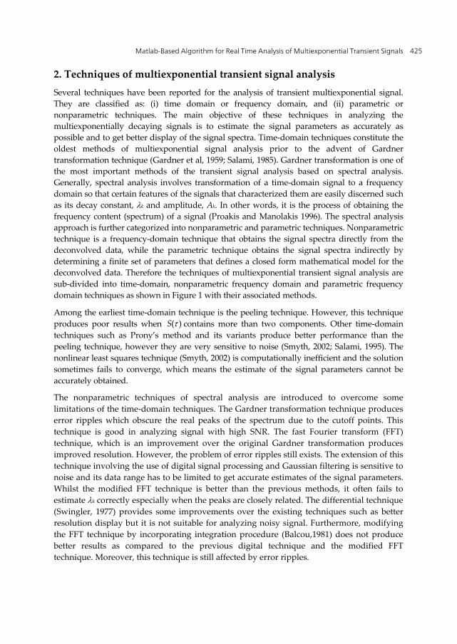
Several techniques have been reported for the analysis of transient multiexponential signal. They are classified as: (i) time domain or frequency domain, and (ii) parametric or nonparametric techniques. The main objective of these techniques in analyzing the multiexponentially decaying signals is to estimate the signal parameters as accurately as possible and to get better display of the signal spectra. Time-domain techniques constitute the oldest methods of multiexponential signal analysis prior to the advent of Gardner transformation technique (Gardner et al, 1959; Salami, 1985). Gardner transformation is one of the most important methods of the transient signal analysis based on spectral analysis. Generally, spectral analysis involves transformation of a time-domain signal to a frequency domain so that certain features of the signals that characterized them are easily discerned such as its decay constant, k and amplitude, Ak. In other words, it is the process of obtaining the frequency content (spectrum) of a signal (Proakis and Manolakis 1996). The spectral analysis approach is further categorized into nonparametric and parametric techniques. Nonparametric technique is a frequency-domain technique that obtains the signal spectra directly from the deconvolved data, while the parametric technique obtains the signal spectra indirectly by determining a finite set of parameters that defines a closed form mathematical model for the deconvolved data. Therefore the techniques of multiexponential transient signal analysis are sub-divided into time-domain, nonparametric frequency domain and parametric frequency domain techniques as shown in Figure 1 with their associated methods.

Among the earliest time-domain technique is the peeling technique. However, this technique produces poor results when ( )S contains more than two components. Other time-domain techniques such as Prony’s method and its variants produce better performance than the peeling technique, however they are very sensitive to noise (Smyth, 2002; Salami, 1995). The nonlinear least squares technique (Smyth, 2002) is computationally inefficient and the solution sometimes fails to converge, which means the estimate of the signal parameters cannot be accurately obtained.

The nonparametric techniques of spectral analysis are introduced to overcome some limitations of the time-domain techniques. The Gardner transformation technique produces error ripples which obscure the real peaks of the spectrum due to the cutoff points. This technique is good in analyzing signal with high SNR. The fast Fourier transform (FFT) technique, which is an improvement over the original Gardner transformation produces improved resolution. However, the problem of error ripples still exists. The extension of this technique involving the use of digital signal processing and Gaussian filtering is sensitive to noise and its data range has to be limited to get accurate estimates of the signal parameters. Whilst the modified FFT technique is better than the previous methods, it often fails to estimate k correctly especially when the peaks are closely related. The differential technique (Swingler, 1977) provides some improvements over the existing techniques such as better resolution display but it is not suitable for analyzing noisy signal. Furthermore, modifying the FFT technique by incorporating integration procedure (Balcou,1981) does not produce better results as compared to the previous digital technique and the modified FFT technique. Moreover, this technique is still affected by error ripples.


Figure 1. Overview of Techniques for Multiexponential signal analysis

Parametric techniques such as Autoregressive (AR), Moving Average (MA) and ARMA models are introduced to the analysis of multiexponential signals to alleviate the drawbacks of the nonparametric techniques. The AR modeling technique requires less computation than the ARMA modeling technique as its model parameters are relatively easy to estimate. However, it is sensitive to noise due to the assumed all-pole model. On the other hand, MA parameters are difficult to estimate and the resultant spectral estimates have poor resolution. Although, the ARMA modeling technique is much better in estimating noisy signal than the AR modeling technique, it requires a lot of computation. A detailed review of these techniques can be obtained in (Jibia, 2009; Salam and Sidek, 2000).


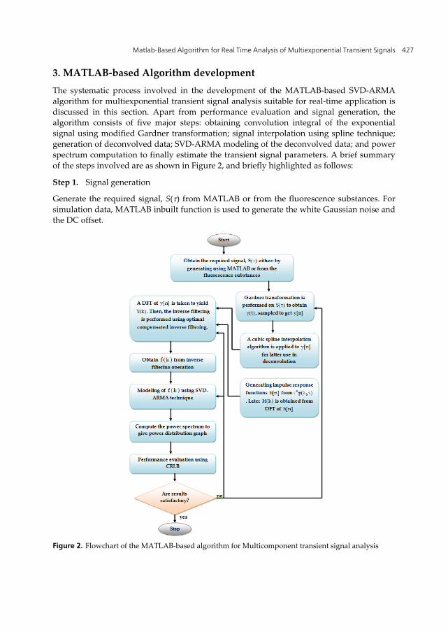
3. MATLAB-based Algorithm development The systematic process involved in the development of the MATLAB-based SVD-ARMA algorithm for multiexponential transient signal analysis suitable for real-time application is discussed in this section. Apart from performance evaluation and signal generation, the algorithm consists of five major steps: obtaining convolution integral of the exponential signal using modified Gardner transformation; signal interpolation using spline technique; generation of deconvolved data; SVD-ARMA modeling of the deconvolved data; and power spectrum computation to finally estimate the transient signal parameters. A brief summary of the steps involved are as shown in Figure 2, and briefly highlighted as follows:

Step 1. Signal generation

Generate the required signal, S() from MATLAB or from the fluorescence substances. For simulation data, MATLAB inbuilt function is used to generate the white Gaussian noise and the DC offset.

Figure 2. Flowchart of the MATLAB-based algorithm for Multicomponent transient signal analysis


Step 2. Signal preprocessing via Gardner transformation:

This involves the conversion of the measured or generated signal ( )S and ( )p to y(t) and h(t) respectively using modified Gardner transformation (Salami and Sidek, 2003). This yields a convolution integral as subsequently described.

In general, equation (1) is expressed as

1

( ) ( ) ( ),M

kkk

S A p n

(2)

where the basis function, p() = exp(-). This equation can also be expressed as

0

( ) ( ) ( ) ( ),S g p d n

(3)

where1

( ) ( ).M

kkk

g A

Both sides of equation (3) are multiplied by in the modified Gardner transformation instead of only in the original Gardner transformation. The value of the modifying parameter, is carefully chosen based on the criteria given by Salami (1995) to avoid poor estimation of the signal parameters because modifies the amplitude of the signal. Salami (1995) suggested to use 0 1 in the analysis of multiexponential signals. According to Salami (1985), the choice of can lead to improved signal parameters estimation as it produces noise reduction effect. The nonlinear transformation = e-r and = et are applied to equation (3), resulting in a convolution integral of the form

( ) ( ) ( ) ( ),y t x h t d v t

(4)

where the output function, y(t) = exp(t) S{exp(t)}, the input function, x(t) = exp{(-1)t}g(e-t), the impulse response function of the system, h(t) = exp(t)p(et) and the additive noise, v(t) = exp(t)n(et).

The discrete impulse response function, h[n] is obtained by sampling αp(λk) at 1/Δt Hz. Later, H(k) is obtained from the discrete Fourier transform (DFT) of h[n]. Next, equation (4) is converted into a discrete-time convolution. This is done by sampling y(t) at a rate of 1/Δt Hz to obtain

max

min

[ ] [ ] [ ] [ ],n

m ny n x m h n m v n

(5)

where the total number of samples, N equals nmax -nmin+1, both nmax and nmin represent respectively the upper and lower data cut-off points. The criteria for the selection of these sampling conditions have been thoroughly discussed by Salami (1987) and Sen (1995) and


these are not discussed further here. Equation (5) forms the basis of estimating the signal parameters since ideally x(n) can be recovered from the observed data by deconvolution. It is necessary to interpolate the discrete time convolution of y[n] since the log samples, n = exp(n∆t) are not equally spaced.

Step 3. Cubic spline Interpolation

The discrete-time signal y[n] obtained in (5) consists of non-equally spaced samples which would be difficult to digitally process. A cubic interpolation is therefore applied to y[n] using MATLAB function ‘spline’ to obtain equally spaced samples of y[n].

Step 4. Generation of deconvolved data

In this stage, deconvolved data is generated from y[n] using optimally compensated inverse filtering due to its ability to handle noisy signal when compared to conventional inverse filtering (Salami,1995).

Conventionally, this is done by taking the DFT of equation (5) to produce:

( ) ( ) ( ) ( )Y k X k H k V k (6)

The deconvolved data, ( )X k

can be obtained by computing Y(k)/H(k), that is

( ) ( )( ) ( ) 0 1( ) ( )

Y k V kX k X k for k NH k H k

(7)

where Y(k), X(k), H(k) and V(k) represent the discrete Fourier transform of y(n), x(n), h(n) and v(n) respectively. This inverse filtering operation is called the conventional inverse filtering. It yields deconvolved data with decreasing SNR for increasing values of k. Therefore, the accuracy of ( )X k

deteriorates when the noise variance level is high.

To overcome this problem, an optimally compensated inverse filtering is introduced. In this approach, H(k) is modified by adding an optimally selected value, into it. This procedure is done according to Riad and Stafford (1980) by initially designing a transfer function, HT (k) that yields a better X

(k) in equation (7), where HT (k) is given by:

2

( )( ) ,| ( )|

TH kH k

H k

(8)

where denotes the complex conjugate. Substituting equation (8) into equation (7) yields

2

( ) ( )( ) ,| ( )|Y k H kX kH k

(9)

which is referred to as the optimally compensated inverse filtering. It is noted that a small value of μ has a very little effect in the range of frequency when |H(k)|2 is significantly


larger than . However, if|H(k)|2 is very small, the effect of μ on the deconvolved data is quite substantial, that is tends to make ( )X k

less noisy. Therefore, μ puts limit on the

noise amplification because the denominator becomes lower bounded according to Dabóczi and Kollár (1996). The parameter μ is carefully selected according to the SNR of the data to obtain good results. The choice of the optimum value of μ according to Salami and Sidek (2001) is best determined by experimental testing.

Equation (9) shows one-parameter compensation procedure, however, multi-parameter compensation is considered in this study. Thus, a regularization operator L(k) is introduced into (8), that is

2 2

( )( )( ) ( )

H kF kH k L k

(10)

where is the controlling parameter and the regularization operator, L(k) is the discrete Fourier transform of the second order backward difference sequence. |L(k)|2 is given as

2 4| ( )| 16sin ,kL kN

(11)

where N is the number of samples. Using both the second and fourth order backward difference operations in equation (10) yield

2 2 4

( )( )( ) ( ) ( )

H kF kH k L k L k

(12)

where 4( )L k denotes the fourth order backward difference operator and , and are the

varied compensation parameters to improve the SNR of the deconvolved data.

Unwanted high frequency noise can still be introduced by this optimally compensated inverse filtering which can make some portion of ( )X k

unusable. Therefore, a good portion

of ˆ ( )X k denoted as f (k), is given as

1

( ) exp( 2 ln ) ( ),M

i ii

f k B j k f V k

(13)

where 1 k 2Nd+1, = / , Nd ( / 2) 1N , Nd is the number of useful deconvolved data points, N is the number of data samples and V(k) is the noise samples of the deconvolved data. Equation (13) is interpreted as a sum of complex exponential signals. The number of deconvolved data points, Nd is carefully selected to produce good results from f (k).

Step 5. Signal parameters estimation using SVD-ARMA modeling

SVD-ARMA algorithm is applied to f(k) to estimate the signal parameters M and k. as it provides consistent and accurate estimates of AR parameters with minimal numerical


problem which is necessary for real-time application. In addition, it is a powerful computational procedure for matrix analysis especially for solving over determined system of equations. The detailed mathematical analysis of this algorithm is reported in (Salami, 1985).

Generally, the ARMA model assumes that f (k) satisfies the linear difference equation (Salami 1985)

1 1

( ) ( ) ( ) ( ) ( )p q

i if k a i f k i b i V k i

(14)

where V(k) is the input driving sequence, f(k) is the output sequence, a[i] and b[i] are the model coefficients with AR and MA model order of p and q respectively. Usually, the white Gaussian noise becomes the input driving sequence in the analysis of exponentially decaying transient signals.

One of the most effective procedures for estimating these model parameters is by solving a modified Yule-Walker equation (Kay and Marple 1981). This procedure is subsequently discussed.

Equation (14) is multiplied by f *(k-m) and taking the expectation yields:

1 0

( ) [ ] ( ) [ ] ( ),p q

ff ffn n

R k a n R k n b n h k m

(15)

where Rff (k) is the autocorrelation function of ( )f k and h(k) is the impulse response function of the ARMA model. Next, considering the AR portion of equation (15) leads to the modified Yule-Walker equation

1

( ) [ ] ( ) 0; 1.p

ff ffn

R k a n R k n k q

(16)

Equation (16) may not hold exactly in practice because both p and q are unknown prior to analysis and Rff (k) has to be estimated from noisy data. This problem is solved by using an SVD algorithm. This algorithm is used by first expressing equation (16) in matrix form as Ra = e with R having elements ( , ) ( 1 ),ff er i l R q i l where 1 i r ; 1 l pe + 1. Note that both pe and qe are the guess values of the AR and MA model order respectively, a is a pe 1 and e is a r 1 error vector with r > pe. The SVD algorithm is applied to R to produce

R = UVT =

1

epH

n n nn

u v (17)

where the r (pe+1) unitary matrix U = [u1 u2 … 1epu ], (pe+1) (pe+1) unitary matrix V = [v1 v2 … 1epv ] and is a diagonal matrix with diagonal elements ( 1, 2 … 1ep ). These diagonal elements are called singular values and are arranged so that 1 > 2 > … > 1ep > 0. Only the


first M singular values will be nonzero so that M+1 = M+2 = … = 1ep = 0. However, M+1 M+2 … 1ep 0 due to noise contamination. The problem is solved by constructing a lower rank matrix RL from R using the first M singular values, that is

RL = UMMVMH

1,

MH

n n nn

u v

(18)

where UM, M and VM are the truncated version of U, and V respectively. The AR coefficients are then estimated from the relation a = -RL#r, where r corresponds to the first column of RL and RL# is given as

RL# 1

1.

MH

n n nn

u v

(19)

The estimated AR coefficients are then used to generate the residual error sequences:

0 0

( ) [ ] * [ ] ( )e ep p

ffl m

k a l a m R k m l

(20)

from which the actual MA parameters are obtained directly from equation (20). However, MA spectra can be obtained from the DFT of the error sequences, (k) . An exponential window is applied to (k) to ensure that the MA spectra derived from the error sequences are positive definite. Next, the ARMA spectrum is computed from

2

( )( )

( )

e

e

pk

k pf

k zS z

A z

(21)

and the desired power distribution of x(t), denoted as Px(t) is obtained by evaluating Sf (z) on

the unit circle exp 2 tz jN t

, that is:

22

exp 1( ) ( ) ( ln ).

M

x f k kj tz kN t

P t S z B t

(22)

Eventually, M and ln k are obtained from Px(t).

Step 6. Graphical presentation of output

Power distribution graph has been used to display the results of multiexponential signal analysis. This is computed from the power spectrum of the resulting output signal from SVD-ARMA modeling method as shown in equation (21).

Step 7. Performance evaluation

The efficiency of the algorithm with SVD-ARMA modeling technique in estimating k correctly is determined by the Cramer-Rao lower bound (CRLB) expressed as:


CRLB ( k )=3/2 2

36(1 0.7( ) )

,kNN SNR

(23)

where N is the number of data points, the CRB(k) is the CRLB for estimating k and SNR equals to divided by the variance of the white Gaussian noise.

The Cramer-Rao lower bound will determine whether the estimator is efficient by comparing the variance of the estimator, var( k

) with the Cramer-Rao lower bound.

Variance that approaches the CRLB is said to be optimal according to Kay and Marple (1981) and Sha’ameri (2000). Consequently, the closer the variance of the estimator is to the CRLB, the better is the estimator.

A MATLAB-mfile code has been written to implement the steps 1 to 6 described above, details of this have been thoroughly discussed in (Jibia, 2009).

4. Integrated MATLAB-labview for real-time implementation

This section discusses the development of proposed integrated Labview-MATLAB software interface for real-time (RT) implementation of the algorithm for multicomponent signal analysis as described in section 3. Real-time signal analysis is required for most practical applications of multicomponent signal analysis. In this study, reference is made to the application to fluorescence signal analysis. A typical multicomponent signal analyzer comprises optical sensor which is part of the spectrofluorometer system, signal conditioning/data acquisition system, embedded processor that runs the algorithm in real-time, and display/storage devices as shown in Figure 3. National Instrument (NI) real-time hardware and software are considered for the development of this system due to its ease of implementation.

Figure 3. Block diagram of the multicomponent signal analyzer prototype.

4.1. Labview real-time module and target

The Labview real-time module (RT-software) together with NI sbRIO-9642 (RT-hardware) has been adopted in this study. The Labview Real-Time software module allows for the creation of reliable, real-time applications which are easily downloaded onto the target hardware from Labview GUI programming tool.


The NI sbRIO-9642 is identical in architecture to CompactRIO system, only in a single circuit board. Single-Board RIO hardware features a real-time processor and programmable FPGA just as with CompactRIO, and has several inputs and outputs (I/O) modules as shown in Figure 4.

System development involves graphical programming with Labview on the host Window computer, which is then downloaded and run on real-time hardware target. Since the algorithm has been developed with MATLAB scripts, an integrated approach was adopted in the programme development as subsequently described.

Figure 4. NI sbRIO-9642 for real-time hardware target

4.2. MATLAB-labview software integration

The developed algorithm with MATLAB scripts was integrated inside Labview for real-time embedded set-up as shown in Figure 5. Labview front-panel and block diagrams were developed with inbuilt Labview math Scripts to run the MATLAB algorithm for the analysis of multicomponent signals. The use of Labview allows for ease of programming, and real-time deployment using the Labview real-time module described in section 4.1. Also, it provides a user friendly software interface for real-time processing of the fluorescence signals.

As shown in Figure 5, the sampled data produced by the spectrofluorometer system are pre-processed by the NI-DAQ Cards. These signals are then read by the embedded real-time software, analyze the signals and display the results in a user friendly manner. The user is prompted to enter the number of samples to be analyzed from the front-panel using the developed SVD-ARMA algorithm.


Figure 5. Block Diagram of the real-time set-up

Generally, the developed algorithm with MATLAB scripts was integrated inside Labview for real-time embedded set-up as follows:

i. Pre-simulation of the MATLAB algorithm inside embedded MATLAB Simulink block: this requires re-structuring of the codes to be compatible for embedded Simulink implementation, and hence deployment inside Labview MathScript. Figure 7 shows the MATLAB Simulink blocks configuration with embedded MATLAB function together with cross-section of the algorithm. The DATA with time vector is prepared inside the workspace and linked to the model input. Figure 10 (a-f) shows the simulation results with experimental data described in section 5.


Figure 6. Lab view Block Diagram

Figure 7. Embedded MATLAB set-up for algorithm simulation


ii. Labview programming: Development of Labview front-panel and block diagram is as shown in Figure 4. In the block diagram programming, the Labview MathScript node is employed to integrate the MATLAB codes in the overall Labview programme. The script (Figure 8) invokes the MATLAB software script server to execute scripts written in the MATLAB language syntax

Figure 8. NI Labview MATLAB script nodes

iii. The integrated software interface is evaluated with the real-time fluorescence data collected from a spectrofluorometer.

5. Sample collection, results and discussion

Due to unavailability of spectrofluorometer system that can be directly linked with the set-up, sampled data collected from fluorescence decay experiment conducted using Spectramax Germini XS system were used to test the performance of the integrated system. The schematic diagram of the spectrofluorometer operation is shown in Figure 9, and itemized as follows:

Step 1. The excitation light source is the xenon flash lamp. Step 2. The light passes through the excitation cutoff wheel. This wheel reduces the

amount of stray light into the movable grating. Step 3. The movable grating selects the desired excitation wavelength. Then, this excitation

light enters a 1.0 mm diameter fiber. Step 4. This 1.0 mm diameter fiber focuses the excitation light before entering the sample in

the micro-plate well. This focusing prevents part of the light from striking adjacent wells.

Step 5. The light enters the wheel and if fluorescent molecules are present, the two mirrors focus the light from the well into a 4.0 mm optical bundles.

Step 6. The movable, focusing grating allows light of chosen emission wavelength to enter the emission cutoff wheel.

Step 7. This emission cutoff wheel will further filter the light before the light enters the photomultiplier tube.

Step 8. The photomultiplier tube detects the emitted light and passes a signal to the instrument’s electronics which then send the signal to the data acquisition system inside the spectrofluorometer.

Three intrinsic fluorophores (Acridine Orange; Fluorescein Sodium and Quinine) were used in the experiment. The details of the substances are given in Table 1.


Acridine Orange Fluorescein Sodium Quinine Molecular formula Manufacturer Molecular weight Purity by HPLC Form Colour Solubility in water Solutility in ethanol

C17H12ClN3 Merck 301.8g/mol 99.1% Solid Orange red 28g/l Soluble

C20H10Na2O5 Merck 376.28 Extra pure Solid Reddish brown 500g/l 140g/l

C20H24N2O2 Merck 324.43 Extra pure Powder, White 0.5g/l 1200g/l

Table 1. Characteristics of the fluorophores samples

The simulation results for Acridine orange, Fluorescein Sodium, Quinine, Quinine plus Arcridine, Fluorescein Sodium plus Acridine orange, and Fluorescein Sodium plus Acridine orange plus Quinin in water are shown in Figure 10 (a-f) respectively.

Figure 11 to Figure 13 show the sample of results obtained from the integrated MATLAB-Labview real-time software which has been developed. Both results of simulation and real-time software interface yield accurate estimates of the fluorescence data as shown in Figure 10-Figure 13, and presented in Table 2. The singular values for each of the samples combination are given in Table 3. The results indicate accurate determination of the constituent samples

Figure 9. Schematic diagram of the SPECTRAMAX Gemini Spectrofluorometer operation (SPECTRAmax®)


Figure 10. Sample simulation results with embedded MATLAB function

(a) Acridine orange (b) Fluorescein Sodium

(c) Quinine (d) Quinine plus Arcridine

(e) Fluorescein Sodium plus Acridine (f) and Fluorescein Sodium plus Acridine plus Quinin


6. Conclusion/Future study

The development of MATLAB-based algorithm for real-time analysis of multicomponent transient signal analysis based on SVD-ARMA modeling technique has been presented in this chapter. To enhance real-time interface and rapid prototyping on target hardware, complementary benefits of MATLAB and Labview were explored to develop real-time software interface downloadable into single board computer by NI Labview. In the absence of the spectrofluorometer system, the developed user friendly software for real-time deployment was validated with the collected real-time data. The obtained results indicate the effectiveness of the proposed integrated software for practical application of the proposed algorithm.

Future direction of this research will be directed towards development of customized spectrofluorometer sub-system that can be directly integrated to the overall system. This will eventually facilitate direct application of the developed algorithm in practical applications involving transient signal analysis. Also, other algorithms based on homomorphic and eigenvalues decomposition developed by the authors in similar study are to be made available as option on the user interface.

Mixture Expected value SVD-ARMA

Percentage error

Acridine orange 0.5978 0.625 4.55

Fluorescein Sodium

-1.4584

-1.438

1.40

Quinine

-0.6419

-0.625

2.63 Acridine Orange + Fluorescein Sodium

0.6539 0.6563 0.37

-1.4584

-1.438

1.40 Acridine Orange +Quinine

0.7750 0.761 1.81

-0.5539

-0.5313

4.08 Acridine Orange + Fluorescein Sodium +Quinine

0.5105 0.5325 4.31 -0.6152 -0.5938 3.48 -1.5260 -1.533 0.46

Table 2. Estimated Log of decay rates and percentage error from fluorescence decay experiment ( In )


Table 3. Singular values for SVD-ARMA using experimental data

Figure 11. Power distributions for Quinine in water


Figure 12. Power distribution Quinine plus Arcridine Sodium in water

Figure 13. Power distribution for Acridine Orange + Fluorescein + Sodium and quinine in water

Author details

Momoh-Jimoh E. Salami, Ismaila B. Tijani and Za’im Bin Ismail Intelligent Mechatronics Research Unit, Department of Mechatronics, International Islamic University Malaysia, Gombak, Malaysia

Abdussamad U. Jibia Department of Electrical/Electronic Engineering, Bayero University Kano, Kano, Nigeria


7. References

Abdulsammad Jibia,2010.“Real Time Analysis of Multicomponent Transient Signal using a Combination of Parametric and Deconvolution Techniques”, A PhD thesis submitted to Department of ECE, IIUM, Malaysia.

Arunachalam, V. (1980). Multicomponent Signal Analysis. PhD dissertation, Dept. of Electrical Engineering, The University of Calgary, Alberta, Canada.

Balcou, Y. (1981). Comments on a numerical method allowing an improved analysis of multiexponential decay curves. International journal of modelling and simulation. 1 (1), 47-51.

Cohn-Sfetcu, S., Smith, M.R., Nichols, S.T. & Henry, D.L. 1975. A digital technique for analyzing a class of multicomponent signals. Processings of the IEEE. 63(10): 1460-1467.

Embedded MATLAB User guide, 2008. Ww.mathworks.com, accessed date: Jan., 2011 Gardner, D.G., Gardner, J.C. & Meinke, W.W. 1959. Method for the analysis of

multicomponent exponential decay curves. The journal of chemical physics. 31(4): 978-986. Gutierrez-Osuna, R., Gutierrez-Galvez, A., & Powar, N. (2003). Transient response analysis

for temperature-modulated hemoresistors. Sensors and Actuators Journal B (Chemical), 93 (1-3), 57-66.

Hildebrad, F.B., (1956). Introduction to numerical analysis. New York: McGraw-Hill. Istratov, A. A., & Vyvenko, O. F. (1999). Exponential Analysis in Physical Phenomena. Rev.

Sci. Instruments, 70 (2), 1233-1257. Isernberg, I., & Dyson, R. D. (1969). The analysis of fluorescence decay by a method of

moments. The Biophysical Journal, 9 (11), 1337-1350. Jibia, A.U., Salami, M.J.E., & Khalifa, O.O. (2009). Multiexponential Data Analysis Using

Gardner Transform . (a draft ISI review journal paper) Jibia, A.U. & Salami, M.J.E. (2007). Performance Evaluation of MUSIC and Minimum Norm

Eigenvector Algorithms in Resolving Noisy Multiexponential Signals. Proceedings of World Academy of Science, Eng. and Tech Vol. 26, Bangok, Thailand. 24-28.

Karrakchou, M., Vidal, J., Vesin, J.M., Feihl, F., Perret, C. & Kunt, M. 1992. Parameter estimation of decaying exponentials by projection on the parameter space. Elsevier Publishers B.V. 27: 99-107.

Kay, S.M. &Marple, S.L. (1981). Spectrum analysis – A modern perspective. Labview usr manual,2010. www.ni.com/pdf/manuals. accessed Jan., 2011

Lakowicz, J.R. 1999. Principles of fluorescence spectroscopy. 2nd Ed. New York: Kluwer Academic/Plenum Publishers.

Nichols, S.T., Smith, M.R. & Salami, M.J.E. (1983). High Resolution Estimates in Multicomponent Signal Analysis (Technical Report). Alberta: Dept. of Electrical Enginering, University of Calgary.

Provencher, S.W. 1976. A Fourier method for the analysis of exponential decay curves. Biophysical journal. 16: 27-39.

Prost, R. & Goutte, R. 1982. Kernel splitting method in support constrained deconvolution for super-resolution. Institut National des Science, France.

Prony, R. (1795). Essai Experimentals et Analytique. J. ecole Polytech., Paris, 1, 24- 76.


Proakis, J.G. & Manolakis, D.G. (2007). Digital signal processing: Principles, algorithms, and applications. New Jersey: Prentice-Hall.

Prony, R. (1795). Essai Experimentals et Analytique. J. ecole Polytech., Paris, 1, 24-76. Provencher, S.W. (1976). A Fourier method for the analysis of exponential decay curves.

Biophysical journal, 16, 27-39. Salami, M.J.E. (1985).Application of ARMA models in multicomponent signal analysis.

Ph.D. Dissertation, Dept. of Electrical Engineering, University of Calgary, Calgary, Canada

Salami, M.J.E. (1995). Performance evaluation of the data preprocessing techniques used in multiexponential signal analysis. AMSE Press. 33 (2), 23-38.

Salami, M.J.E. (1999). Analysis of multicomponent transient signal using eigen- decomposition based methods.Proc. Intern. Wireless and Telecom. Symp.,3 (5), 214-217.

Salami, M.J.E., & Bulale, Y.I. (2000). Analysis of multicomponent transient signals: A MATLAB approach. 4th International Wireless and Telecommunications Symposium/Exhibition, 253-256.Proceedings of the IEEE, 69 (11), 1380-1419.

Salami M.J.E. & Ismail Z. (2003). Analysis of multiexponential transient signals using interpolation-based deconvolution and parametric modeling techniques. IEEE International conference on Industrial Technology, 1, 271-276.

Salami M.J.E. and Sidek S.N. (2000). Performance evaluation of the deconvolution techniques used in analyzing multicomponent transient signals. Proc. IEEE Region 10 International Conference on Intelligent System and Technologies for the New Millennium (TENCON 2000), 1, 487-492.

Sarkar, T.K., Weiner, D.D. & Jain V.K. (1981). Some mathematical considerations in dealing with the inverse problem. IEEE transactions on antennas and propagation, 29 (2), 373-379.

Schlesinger, J. (1973). Fit to experimental data with exponential functions using the fast Fourier transform. Nuclear instruments and methods. 106, 503-508.

Sen, R. 1995. On the identification of exponentially decaying signals. IEEE Transaction Signal Processing. 43(8): 1936-1945.

Smyth, G.K. (2002). Nonlinear regression. Encyclopedia of environmetrics. 3, 1405-1411. SPECTRAmax® GEMINI XS product literature. http://www.biocompare.com/Product-

Reviews/41142-Molecular-Devices-8217-SPECTRAmax-GEMINI-XS-Microplate-Spectrofluorometer/ accessed on December, 2008.

Swingler, D.N. (1999). Approximations to the Cramer-Rao lower bound for a single damped exponential signal. . Signal Processing, 75 (2), 197-200.

Trench, W.F. (1964). An algorithm for the inversion of finite Toeplitz matrices. J. SIAM, 12 (3), 515-522.

Ulrych, T.J. (1971). Application of homomorphic deconvolution to seismology. Geophysics, 4 (36), 650-660.

matlab-based algorithm for real time analysis of...

Documents