matlab-ii: computing, programming and data analysisylataus/matlab/matlabii.pdf · matlab-ii:...

Matlab-II: Computing, Programming and Data Analysis

Division of Statistics and Scientific Computation College of Natural Sciences

Instructor: Yla Tausczik [email protected]

Division of Statistics and Scientific Computing (SSC)

• Classes (under & grad)

• Portfolio Programs (under & grad)

• Free Consulting

• Software tutorials

Division of Statistics and Scientific Computing (SSC)

Matlab Short Course Structure

Matlab-I Getting Started

Matlab-II Computing and Programming

Matlab-III Data Analysis and Graphics

Matlab-IV Modeling and Simulation

Matlab II Outline

Part I Computing Data Analysis

10 min break

Part II Graphing Programming

Q & A

Matlab I: Basic Concepts

Everything is a matrix Numerical not symbolic calculations Interpreter vs M-files Basic Functions

Tutorial Files Matlab II

http://ssc.utexas.edu/software/software-tutorials

Under Matlab II, download files Under Matlab III, download files

Matlab Computing & Data Analysis

Constants and functions Operational manipulations Descriptive Statistics Mathematical & Statistical

Techniques

Matlab Constants and Functions

Built-in Constants • Machine independent

o inf, NaN, i, j, pi o ans (most recent unassigned input)

• Machine or seed dependent o eps, realmin, realmax o rand, randn (overwritten with each call)


Extended built-in Mathematical Functions Also many distributed with Matlab as m-files

• Trigonometric inverses: a prefix → arc, h suffix → hyperbolic o asin, acos, atan, acsc, asec, acot o asinh, acosh, atanh, acsch, asech, acoth

• Specialized o airy, beta, legendre o various bessel function types, etc.

• Miscellaneous o sqrt, factorial, gamma, erf, exp, log, log2, log10

• Built-in : m-file has description but no source code • Distributed: m-file has annotated source code


More specialized math functions

• Help > Function Browser

• Function tool fx on left bar of Command Window Only available starting with Matlab R2008b

• Help > Product Help > Symbolic Math Toolbox > Function Reference > Specialized Math dirac, heaviside, …

Symbolic Math Toolbox needs to be installed

Matlab Computation

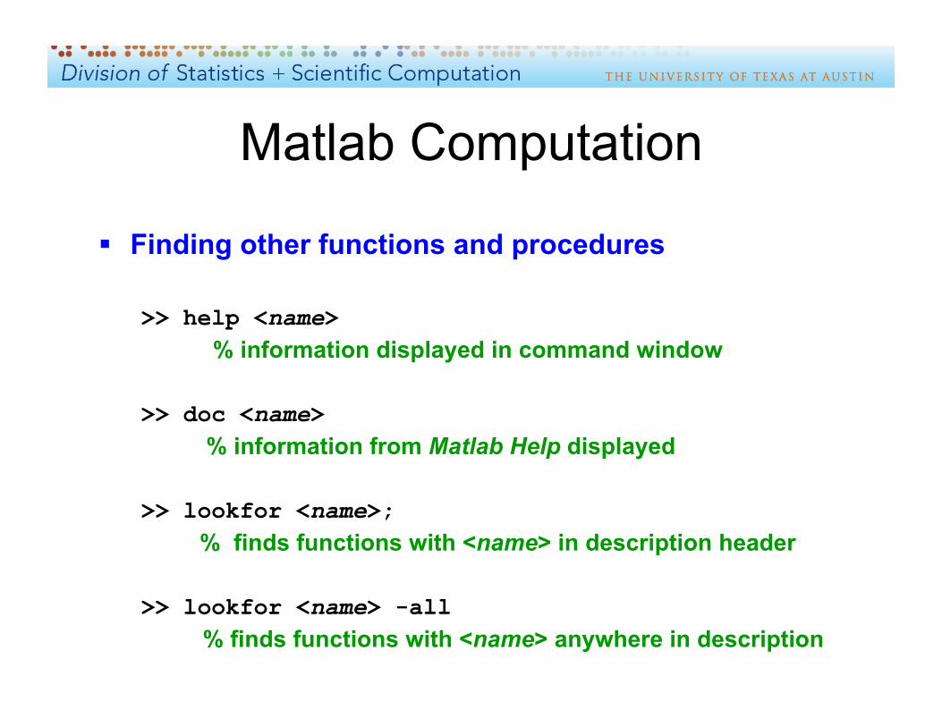
Finding other functions and procedures

>> help <name> % information displayed in command window

>> doc <name> % information from Matlab Help displayed

>> lookfor <name>; % finds functions with <name> in description header

>> lookfor <name> -all % finds functions with <name> anywhere in description

Matlab Computation

Built-in vectors

>> x = linspace(a,b,n); % default n = 100 % linear spacing a → b, row vector

>> y = logspace(a,b,n); % default n = 50 % logarithmic spacing 10a → 10b, row vector

Built-in matrices

>> M = magic(n); % n by n magic square >> N = pascal(n); % n by n Pascal triangle

Matlab Constants and Functions Characterization Functions

• Real numbers o factor(x) % prime number component vector o gcd(x,y), lcm(x,y), round(x), ceil(x), floor(x)

• Complex numbers [of form x = a+bi or x = a+bj] o abs(x), conj(x), real(x), imag(x)

• Logicals [evaluate to 0 (false) or 1 (true)] o isprime(x), isreal(x), isfinite(x), isinf(x), … x is a logical variable, e.g., x = (5 + 4 >= 6)

Matlab Constants and Functions Characterization Functions

• Matrices and vectors o length, size, det, rank, inv, trace, transpose, ctranspose o eig, svd, fft, ifft

• Matrix operation functions end with letter 'm'

o sqrtm, B = sqrtm(A) → B*B = A not sqrt(A(1,1)) = B(1,1), etc.

o expm B = expm(A) → eye(n) + A + (1/2!)*A*A + (1/3!)*A*A*A + … = B

o logm A = logm(B) → expm(A) = B

Matlab Computation

Compound Matrix Expressions • Created by the user

o from built-in components o from user-created simpler components

Concatenation of objects:

P = M^2 - 2.*(M*N)+ N^2

Nesting of groupings: Q = 1./(M./(N + 1./M))

Composition of functions: R = inv(sqrtm(cosh(M)))

Matrix Operator Properties

Associative law • (A+B)+C == A+(B+C) % true • (A.*B).*C == A.*(B.*C) % true • (A*B)*C == A*(B*C) % true

Distributive law • (A + B).*C == A.*C + B.*C % true • (A + B)*C == A*C + B*C % true

Commutative Law • A + B == B + A % true • A.*B == B.*A % true • A*B == B*A % not true in general

Matlab Computation

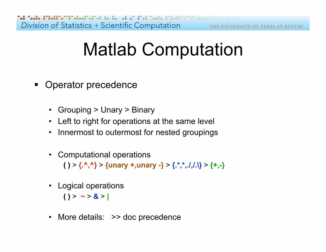
Operator precedence

• Grouping > Unary > Binary • Left to right for operations at the same level • Innermost to outermost for nested groupings

• Computational operations ( ) > {.^,^} > {unary +,unary -} > {.*,*,./,/.\} > {+,-}

• Logical operations ( ) > ~ > & > |

• More details: >> doc precedence

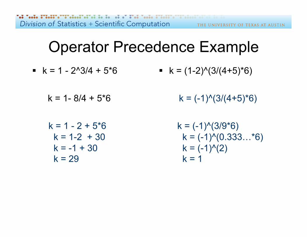
Operator Precedence Example k = 1 - 2^3/4 + 5*6 k = (1-2)^(3/(4+5)*6)

k = 1- 8/4 + 5*6

k = 1 - 2 + 5*6 k = 1-2 + 30 k = -1 + 30 k = 29

k = (-1)^(3/(4+5)*6)

k = (-1)^(3/9*6) k = (-1)^(0.333…*6) k = (-1)^(2) k = 1

Operator Precedence Example k = 1 - 2^3/4 + 5*6

k = 1- 8/4 + 5*6 k = 1 - 2 + 5*6 k = 1-2 + 30 k = -1 + 30 k = 29

^ is the first step

k = (1-2)^(3/(4+5)*6) k = (-1)^(3/(4+5)*6) k = (-1)^(3/9*6) k = (-1)^(0.333…*6) k = (-1)^(2) k = 1

^ is the last step

Finite Number Representation

Decimal expansions rounded off if too long

Irrational numbers rounded off

Consequences can include unexpected results • Commutivity of addition

t = 0.4 + 0.1 - 0.5 → 0 u = 0.4 - 0.5 + 0.1 → 2.7756e-017 t == u → logically False

Logical relationships may not be as expected • cos(2*pi) = = cos(4*pi) → logically True • sin(2*pi) = = sin(4*pi) → logically False (but mathematically True)

Matrix Vectorized Computation Example: Square matrix elements

Vectorized >> B = A.^2

Scalar Loop >> for n = 1:3 for m = 1:3 B(n,m) = (A(n,m)).^2 end end

Data Analysis

Uniform • uniform_sample = rand(100,1).*(b-a)+a

Normal • normal_sample = randn(100,1).*σ + µ

Poisson • poisson_sample = poissrnd(λ,100,1)

Descriptive Statistics

Central tendency variables of vectors • mean, median, var, std (of vector elements)

Operations are on the elements of a vector

If a = [1 2 3] then median(a) → 2

Independent operations on matrix columns

1 2 3 If A = 2 4 9 then mean(A) → 3 5 4

6 9 0


More collective element properties • sum, prod • min, max

► Position of min or max can be obtained, e.g.

>> b = [5 4 3 2 3 4];

>> [bmin_value bmin_position] = min(b)

bmin_value = 2 bmin_position = 4

Note: operations are on absolute values if any elements are complex


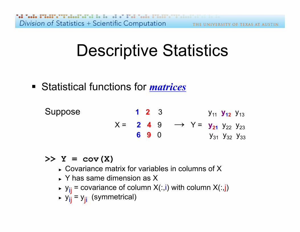
Statistical functions for matrices

Suppose 1 2 3 y11 y12 y13

X = 2 4 9 → Y = y21 y22 y23 6 9 0 y31 y32 y33

>> Y = cov(X) ► Covariance matrix for variables in columns of X ► Y has same dimension as X ► yij = covariance of column X(:,i) with column X(:,j) ► yij = yji (symmetrical)


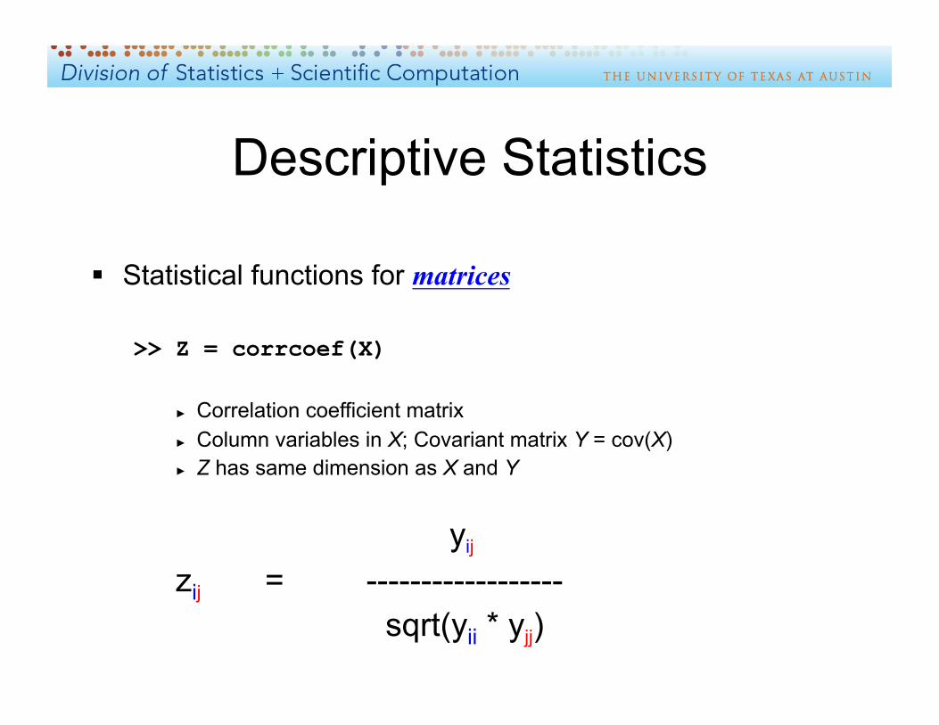
Statistical functions for matrices

>> Z = corrcoef(X)

► Correlation coefficient matrix ► Column variables in X; Covariant matrix Y = cov(X) ► Z has same dimension as X and Y

yij

zij = ------------------ sqrt(yii * yjj)

Descriptive Statistics Exercises with statistical descriptors -- data matrix from wireless.xls

• Find mean quarter hour volume for days of the week >> mean(data)

• Find median quarter hour volume on Wednesdays >> median( data(:,4) )

• Find sums of volume for quarter hours ► Transpose the data matrix first – operations by column >> v = transpose( sum (transpose(data) ) )

• Find day of minimum intraday variance >> [minvalue minday] = min( var(data) )

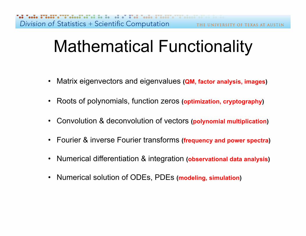
Mathematical Functionality

• Matrix eigenvectors and eigenvalues (QM, factor analysis, images)

• Roots of polynomials, function zeros (optimization, cryptography)

• Convolution & deconvolution of vectors (polynomial multiplication)

• Fourier & inverse Fourier transforms (frequency and power spectra)

• Numerical differentiation & integration (observational data analysis)

• Numerical solution of ODEs, PDEs (modeling, simulation)

Eigenvectors and Eigenvalues

Ax = λx • x eigenvector • λ eigenvalue

Defined for a square matrix A

• Number of eigenvalues and eigenvectors equals the dimension n

o Repeated (degenerate) eigenvalues possible

• Eigenvalues are roots of a polynomial o Defining polynomial det(A – λ*eye(n)) = 0 o n degree polynomial in λ, n roots: λ1 … λn


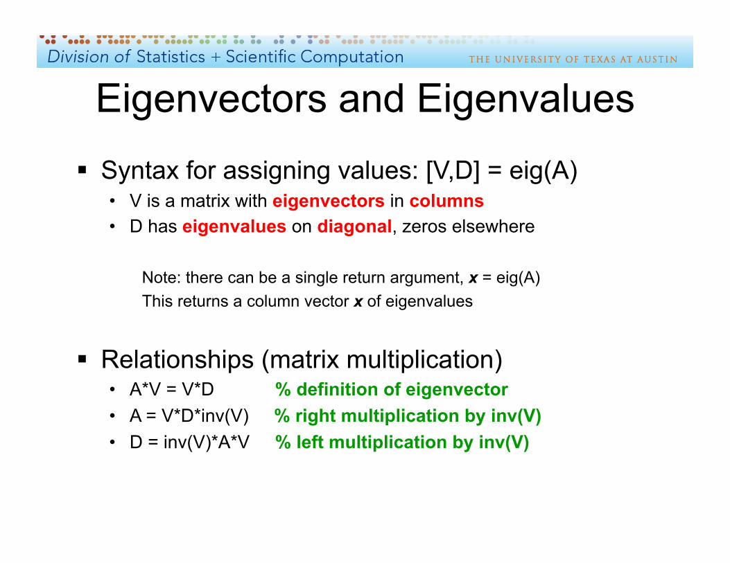
Syntax for assigning values: [V,D] = eig(A) • V is a matrix with eigenvectors in columns • D has eigenvalues on diagonal, zeros elsewhere

Note: there can be a single return argument, x = eig(A) This returns a column vector x of eigenvalues

Relationships (matrix multiplication) • A*V = V*D % definition of eigenvector • A = V*D*inv(V) % right multiplication by inv(V) • D = inv(V)*A*V % left multiplication by inv(V)


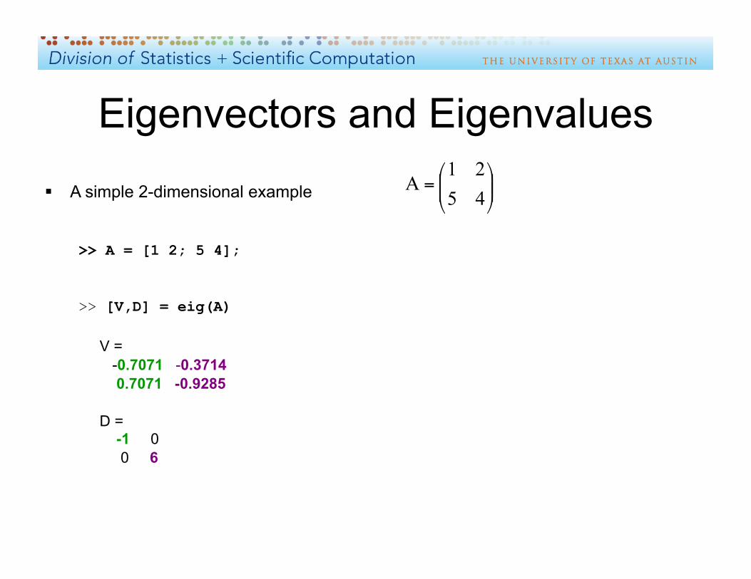
A simple 2-dimensional example

>> A = [1 2; 5 4];

>> [V,D] = eig(A)

V = -0.7071 -0.3714 0.7071 -0.9285

D = -1 0 0 6

Roots and Zeros

Polynomial notation is a coefficient vector • Example: >> p = [ 1 0 -4 ]

o represents (1.*x^2 + 0.*x^1 + (– 4).*x^0) – i.e., x2 – 4

• (n+1) elements for an n degree polynomial o descending ordering by power

• n elements in a corresponding roots vector o Generated as a column vector with roots function

► Example: >> q = roots(p)

• Can be created from a vector of its roots o Generated as a row vector with poly function

► Example: >> r = poly(q)

Roots and Zeros

roots and poly are inverses of each other • If q = roots(p) then

r = poly(q) = poly(roots(p)) = p s = roots(r) = roots(poly(q)) = q

roots of a scalar z >> p = [1 0 0 0 0 … 0 0 -z ]; % vector of length n + 1 Note: this represents xn = z >> q = roots(p) % column vector with all nth roots of z

Roots and Zeros

Function zeros are equivalent to polynomial roots

• The fzero function is a function of a function o It finds the closest argument with function value 0

• A starting point or search range needs to be specified o Start point must be real and finite o Search range limits need function values of opposite sign o Syntax:

>> fz = fzero(@function, start) >> fz = fzero('function', [lower upper])

Roots and Zeros

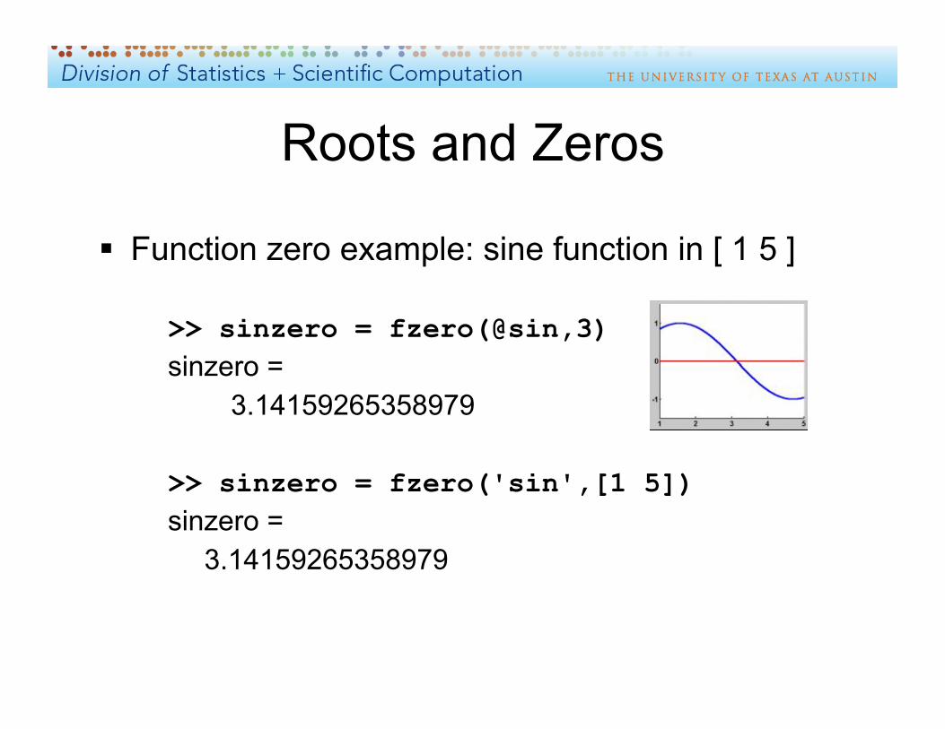
Function zero example: sine function in [ 1 5 ]

>> sinzero = fzero(@sin,3) sinzero = 3.14159265358979

>> sinzero = fzero('sin',[1 5]) sinzero = 3.14159265358979

Convolution and Deconvolution

Convolution is like polynomial multiplication

Polynomial example of multiplication: (using algebra) c(x) = a(x).*b(x) = (2x2 + 3x + 4).*(1x2 – 4x + 7) c = 2x4 – 5x3 + 6x2 + 5x + 28

Equivalent convolution example: >>c = conv([2 3 4], [1 -4 7])% i.e.,conv(a,b)

c = [ 2 -5 6 5 28 ]

Deconvolution is the inverse of convolution >> g = conv(f,h)

>> h = deconv(f,g) >> f = deconv(h,g)

Fast Fourier Transform (FFT) The fft function transforms vector elements

• Transform: [x1 x2 …xN] → [X1 X2 … XN]

The ifft function is an inverse transform • Inverse: [X1 X2 … XN] → [x1 x2 …xN]

Fast Fourier Transforms

Differentiation and Integration

Polynomial derivatives

• Derivatives can be erratic with experimental data o Optional initial smoothing with function polyfit o Syntax: >> p = polyfit(x,y,n)

► Least squares fit to polynomial of degree n ► Vector elements are descending power coefficients

• For polynomial coefficent vector, use polyder o polyder(x) → derivative polynomial vector o Dimension one less than argument vector (final 0 omitted) o Based on dxn/dx = nxn-1 o Second derivative: polyder(polyder(x))


Example: >> x = 0:0.1:2*pi >> y = sin(x)

>> p = polyfit(x,y,5) >> y2 = polyval(p,x)

>> plot(x,y) >> plot(x,y2)

>> w = polyder(p)

>> yderiv = polyval(w,x)

>> plot(x,yderiv)


Non-polynomial numerical derivatives • Approximation using the diff function

o The diff function creates a vector of differences o Differences are of consecutive argument elements o Example: x = [ 1 2 4 7 11 ] and y = [ 1 3 9 21 41 ]

► diff(x) = [ (2-1) (4-2) ( 7- 4) (11- 7 )] = [ 1 2 3 4 ] ► diff(y) = [ (3-1) (9-3) (21-9) (41-21) ] = [ 2 6 12 20 ]

o Numerical derivative dy/dx (very crude): >> yderiv = diff(y)./diff(x) = [ 2 3 4 5 ]

o Second derivative (even more crude): >> yderiv2 =diff(diff(y)./diff(x))./diff(diff(x))


Example: >> x = 0:0.1:2*pi >> y = sin(x)

>> dx = diff(x) >> dy = diff(y)

>> yderiv2 =dy./dx

>> x2 = x(1:end-1)+dx./2

>> plot(x2,yderiv2)

Differentiation and Integration Numerical integration with the polyint function

• Argument is a polynomial coefficient vector o Non-polynomials might be approximated with polyfit o Generated from

o Syntax: >> y = polyint(x,c) o Default constant of integration is c = 0

Differentiation and Integration Numerical integration with the quad function

• Syntax: quad('function_name', lower, upper) o Function name can be user defined in an m-file o Uses an adaptive Simpson’s Rule for quadrature o Example:

>>area = quad('x.^2 - 6.*x + 5', 1, 5) area = -10.6667

o Function does not need to be a polynomial >>area = quad('sin',0,pi) area = 1.99999999619084

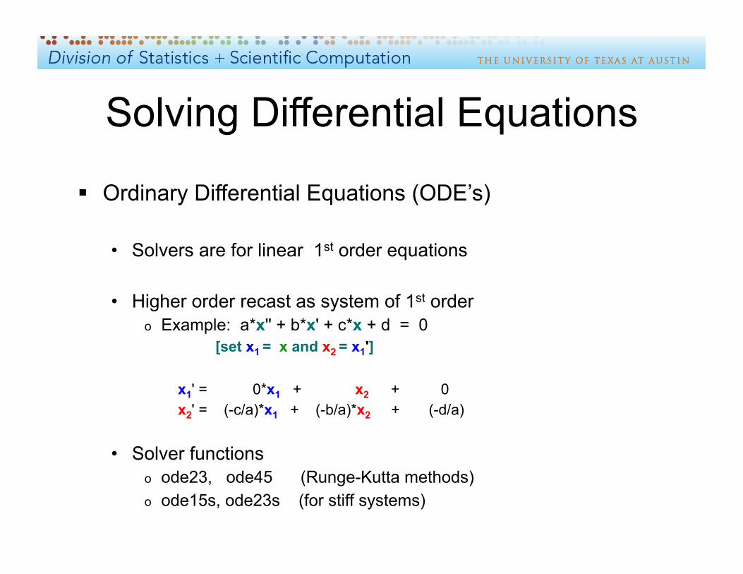
Solving Differential Equations

Ordinary Differential Equations (ODE’s)

• Solvers are for linear 1st order equations

• Higher order recast as system of 1st order o Example: a*x'' + b*x' + c*x + d = 0

[set x1 = x and x2 = x1']

x1' = 0*x1 + x2 + 0 x2' = (-c/a)*x1 + (-b/a)*x2 + (-d/a)

• Solver functions o ode23, ode45 (Runge-Kutta methods) o ode15s, ode23s (for stiff systems)

Statistical Functionality

• Regression (inferential statistics, model fitting)

• Matlab Statistical Toolbox (inferential statistics)

Regression and Curve Fitting

Polynomial function fitting with polyfit • Syntax:

>> polycoeffs = polyfit(x, y, n) x is a vector of independent variable values y is a vector of dependent variable values n is the order of the polynomial desired

► select n = 1 for linear regression, n = 2 for quadratic, etc.

• Function evaluation with polyval >> ycalc = polyval(polycoeffs, x) >> residuals = ycalc - y


Exercise • Fit the curve for population center migration

► Examine the m file popcenterfit.m * Plot of north latitude as a function of west longitude * Coefficients for linear fit (ordinary regression) * Coefficients for cubit fit (cubic regression) * Plot of linear and cubic regression lines

► Execute the script ► Compare linear and cubic fits on plot ► Look at sum of squares of residuals


Linear >>X = [ones(length(west)),west] >>[b,bint,r,rint,stats] = regress(north,X)

Cubic >> X3 =

[ones(length(west)),west,west.^2,west.^3] >>[b,bint,r,rint,stats] = regress(north,X3)

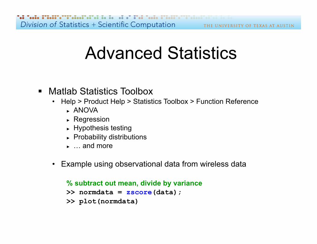
Advanced Statistics

Matlab Statistics Toolbox • Help > Product Help > Statistics Toolbox > Function Reference

► ANOVA ► Regression ► Hypothesis testing ► Probability distributions ► … and more

• Example using observational data from wireless data

% subtract out mean, divide by variance >> normdata = zscore(data); >> plot(normdata)

Matlab Visualization & Programming

Graphing Calling M-file scripts and functions Flow control and string evaluation Debugging

Graphics and Data Display Matlab demo data file: sunspot.dat

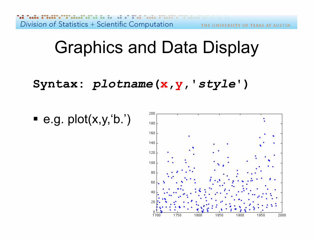
Graphics and Data Display

Syntax: plotname(x,y,'style')

e.g. plot(x,y,‘b.’)


Exercise • Load the file sunspot.dat

• Equate variable year with the first column Use command: >> year = sunspot(:,1);

• Equate variable spots with second column

• Make a simple line plot of spots vs. year

• Superimpose data points as red asterisks * Use 'r*' for 'plotstyle’

• Create a title: >> title(‘Sunspots by year’)

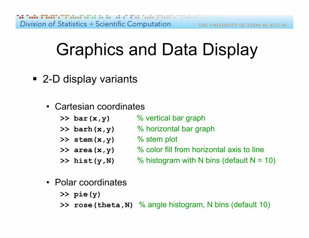
Graphics and Data Display 2-D display variants

• Cartesian coordinates >> bar(x,y) % vertical bar graph >> barh(x,y) % horizontal bar graph >> stem(x,y) % stem plot >> area(x,y) % color fill from horizontal axis to line >> hist(y,N) % histogram with N bins (default N = 10)

• Polar coordinates >> pie(y) >> rose(theta,N) % angle histogram, N bins (default 10)


Layout options

• Single window ► Replace data

>> hold off;

► Overlay on previous data >> hold on;

► Subplots – rectangular array

• Multiple windows >> figure(n) % nth plot >> figure(n+1) % (n+1)th plot

-- etc. --


Subplot syntax

>> subplot(i,j,k), plotname(x,y,’style’)

• i is the number of rows of subplots in the plot • j is the number of columns of subplots in the plot • k is the position of the plot

► Sequential by rows, then columns ► Example: subplot(2, 2, N)

N = 1 for upper left, N = 2 for upper right N = 3 for lower left, N = 4 for lower right

Graphics and Data Display Subplot layout positions (2 x 3 example)


Exercise: Make subplot array for spots vs. year

area(year, spots) % place in upper left bar(year, spots) % place in upper right barh(year, spots) % place in lower left hist(spots) % place in lower right

----------------------------------

>> subplot(2,2,1), area(year,spots) % etc.

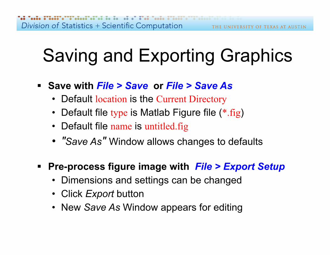
Saving and Exporting Graphics Save with File > Save or File > Save As

• Default location is the Current Directory • Default file type is Matlab Figure file (*.fig) • Default file name is untitled.fig • "Save As" Window allows changes to defaults

Pre-process figure image with File > Export Setup • Dimensions and settings can be changed • Click Export button • New Save As Window appears for editing

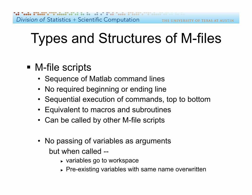
Types and Structures of M-files

M-file scripts • Sequence of Matlab command lines • No required beginning or ending line • Sequential execution of commands, top to bottom • Equivalent to macros and subroutines • Can be called by other M-file scripts

• No passing of variables as arguments but when called --

► variables go to workspace ► Pre-existing variables with same name overwritten

Types and Structures of M-files

M-file functions • First line is function declaration

o Function elements to be returned identified o Variables can be imported as arguments o Function name should correspond to m-file name o First line format for m-file function_name.m :

function [f1 f2 …] = function_name(a1,a2,…)

• Computed function element values returned • Can be called by other m-file functions • Can call themselves (recursion) • Have their own local workspaces

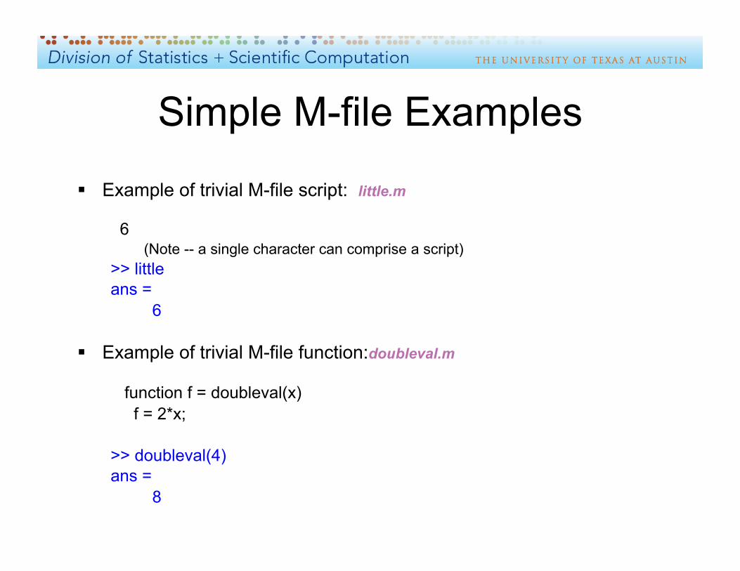
Simple M-file Examples

Example of trivial M-file script: little.m

6 (Note -- a single character can comprise a script)

>> little ans = 6

Example of trivial M-file function:doubleval.m

function f = doubleval(x) f = 2*x;

>> doubleval(4) ans = 8

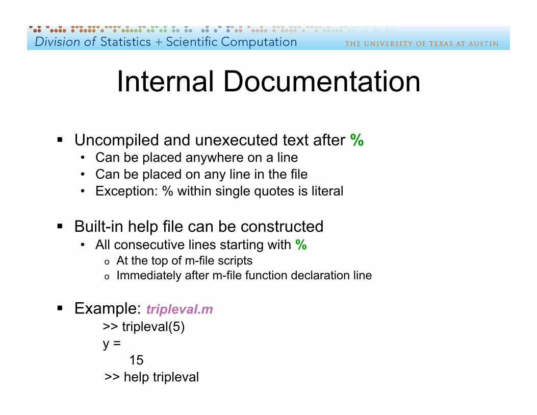
Internal Documentation

Uncompiled and unexecuted text after % • Can be placed anywhere on a line • Can be placed on any line in the file • Exception: % within single quotes is literal

Built-in help file can be constructed • All consecutive lines starting with %

o At the top of m-file scripts o Immediately after m-file function declaration line

Example: tripleval.m >> tripleval(5) y = 15 >> help tripleval

Passing function variables

Variables within functions are local • Can be shared if declared global

o Syntax: global var1

o Global variable needs global declaration ► in calling script before it is defined or used ► In called function code before it is defined or used

o Can share value among subfunctions in a function ► Each subfunction must declare it global

Subfunctions

Functions can have private subfunctions

• Embedded within the parent function • No separate m-file • First line has same format • Last line of subfunction must be end

o Subfunctions can have their own subsubfunctions

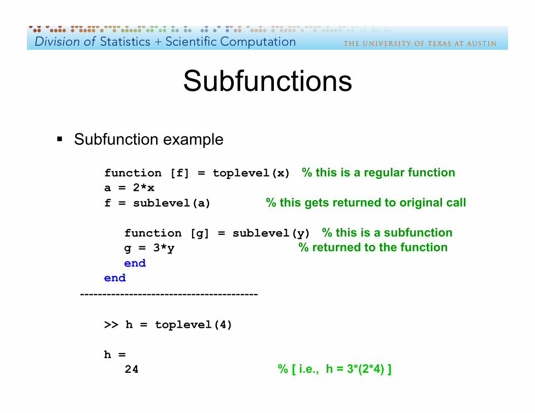
Subfunctions

Subfunction example

function [f] = toplevel(x) % this is a regular function a = 2*x f = sublevel(a) % this gets returned to original call

function [g] = sublevel(y) % this is a subfunction g = 3*y % returned to the function end end

----------------------------------------

>> h = toplevel(4)

h = 24 % [ i.e., h = 3*(2*4) ]

Sharing variable values

Calling script p

Global q

Function 1 u

Global q,x

Function 2 v

Global x

Subfunction A w

Global x

Subfunction B y

Global q

Function 3 s

SubSubfunction D z

Global q

Function3 s

Subfunction C t

Subfunction C t

Dark orange knows about value of q Blue knows about value of x Pink knows about value of both q and x

Passing function variables

Programming example : xseven.m • Long method of multiplication by 7 x*7

function

= x*4 + x*3 subfunction subfunction

= x *1 + x*3 + x*1 + x*2 global subfunction global subsubfunction

= [ x*1 + (x*1 + x*2) ] + [ x *1 + x*2 ] subsubfunction subsubfunction

7 = [ 1 + ( 1 + 2) ] + [ 1 + 2 ]

Function Recursion Function scripts can call themselves

• Example - finding a triangular number: triangular.m t(1) t(2) t(3) t(4) 1 1 1 1 2 3 2 3 2 3 4 5 6 4 5 6 7 8 9 10 t(1) = 1, otherwise t(n) = n + t(n-1) = n + ( (n-1) + t(n-2)) =

= n + ( (n-1) + ( (n-2) + t(n-3)) ...

String Evaluation : eval Matlab can parse strings as functions

• Define an expression or function as a string o Examples:

>> var35 = 'xseven(5)';

>> x = 'sin(n)';

• Evaluate with eval function >> thirtyfive = eval(var35)

thirtyfive = 35

>> n = 1; >> y = eval(x) y = 0.84147 % i.e., [sin(1)]

• eval loads the entire command interpreter

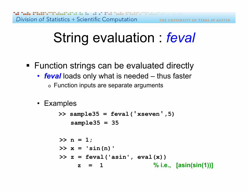
String evaluation : feval

Function strings can be evaluated directly • feval loads only what is needed – thus faster

o Function inputs are separate arguments

• Examples >> sample35 = feval('xseven',5)

sample35 = 35

>> n = 1; >> x = 'sin(n)' >> z = feval('asin', eval(x))

z = 1 % i.e., [asin(sin(1))]

Storage and transport variables Easy to reference contents

• Multi-dimensional arrays o Elements need to be of same type (number or char) o Parentheses as delimiters, e.g. : A(4,2,5,1) = 16;

Awkward to reference contents

• Cells o Array of arrays – each can be of a different type o Curly braces as delimiters, e.g. : B{2,3} = [1 2; 3 4];

• Structures o Root name with extensions and index – types can be mixed o Periods as delimiters, e.g. : C.color(2,1:5) = 'green'; C.colornum(2,1:3) = [0 1 0];

Multidimensional Arrays Matlab matrix operations are on 2-D arrays

• Storage is by concatenation of columns (1-dimensional)

Suppose

1 2 3 A = 4 5 6 7 8 9

• Stored as [ 1 4 7 2 5 8 3 6 9].' • Thus A(2,3) = A(8) = 6

Multidimensional Arrays Equal rows can be concatenated horizontally Equal columns can be concatenated vertically

Examples: consolidation by concatenation

>> E = [ A B ]; % (2 rows, 6 columns) >> F = [ C; D ]; % (6 rows, 2 columns)

Multidimensional Arrays Arrays can be expanded by assignment

• Thus size adjustments can be made for concatenation

Reference outside boundary gives error >> x = A(3,2); ??? Index exceeds matrix dimensions

Assignment outside boundary gives expansion >> A(3,2) = 1;

Debugging

Matlab has a built-in debug help • Error messages in Command Window (red font) • Editor has debug item on navigation bar

o Choose Run from menu ► Diagnostic messages in Command Window

Programmer can modify code • Remove output suppression from semi-colons • Insert markers for screen display: disp( 'marker_text ')

The db* functions can be used • Allows pauses to examine status

o >> dbstop at 40 in badfile.m (stops execution at line 40) >> dbcont (continues execution until next stop point) >> dbquit (exits debugging mode)

Debugging

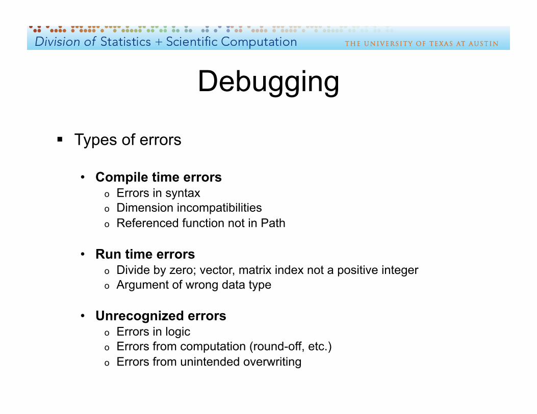
Types of errors

• Compile time errors o Errors in syntax o Dimension incompatibilities o Referenced function not in Path

• Run time errors o Divide by zero; vector, matrix index not a positive integer o Argument of wrong data type

• Unrecognized errors o Errors in logic o Errors from computation (round-off, etc.) o Errors from unintended overwriting

Debugging

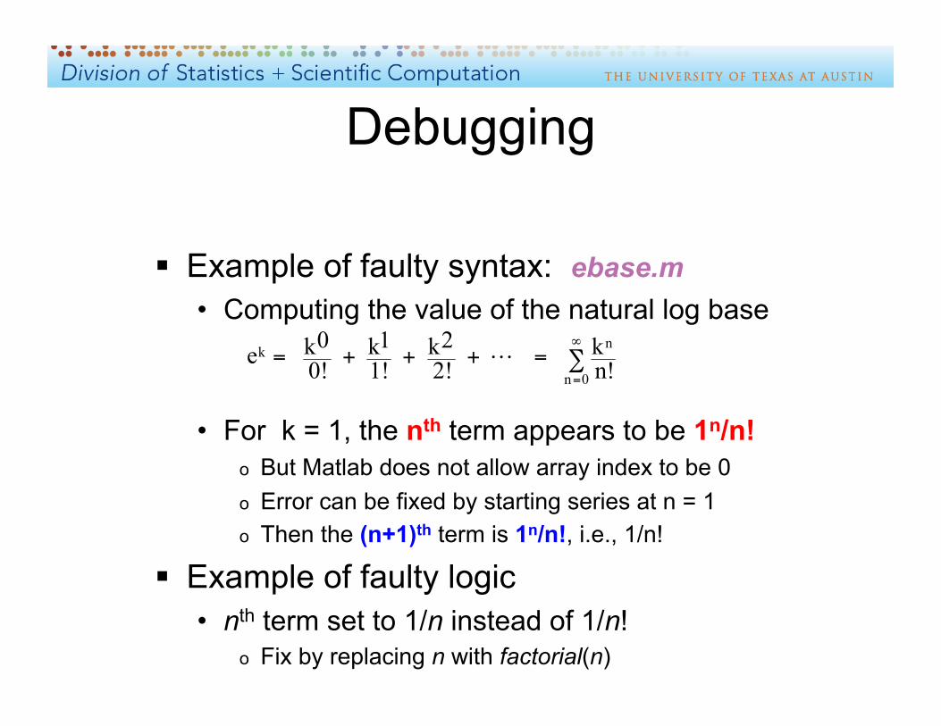
Example of faulty syntax: ebase.m • Computing the value of the natural log base

• For k = 1, the nth term appears to be 1n/n! o But Matlab does not allow array index to be 0 o Error can be fixed by starting series at n = 1 o Then the (n+1)th term is 1n/n!, i.e., 1/n!

Example of faulty logic • nth term set to 1/n instead of 1/n!

o Fix by replacing n with factorial(n)

Debugging

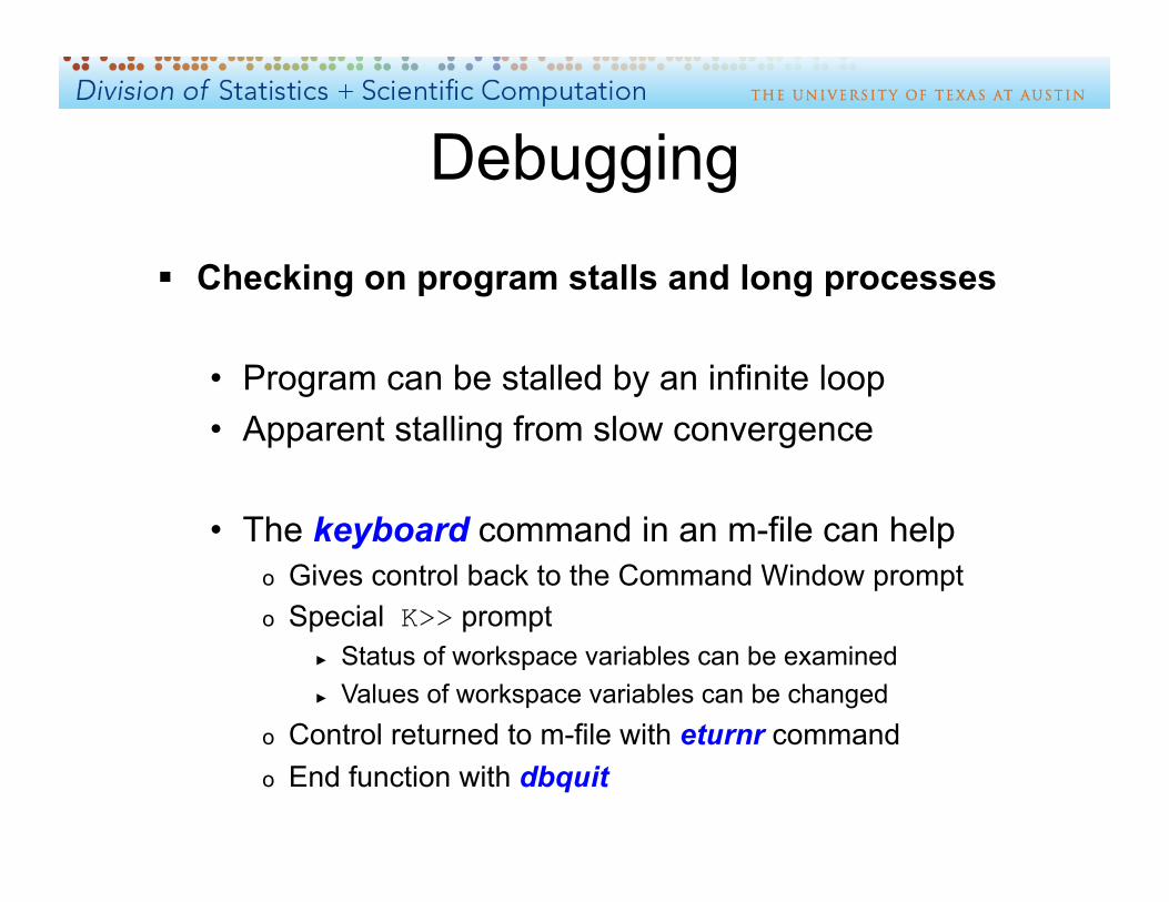
Checking on program stalls and long processes

• Program can be stalled by an infinite loop • Apparent stalling from slow convergence

• The keyboard command in an m-file can help o Gives control back to the Command Window prompt o Special K>> prompt

► Status of workspace variables can be examined ► Values of workspace variables can be changed

o Control returned to m-file with eturnr command o End function with dbquit

Debugging

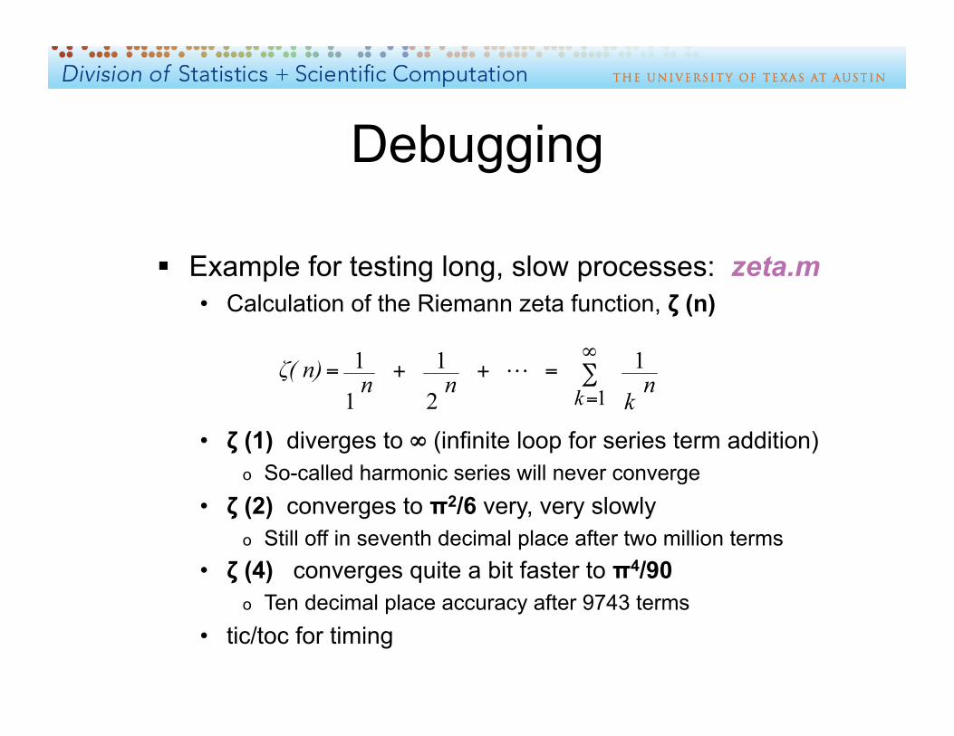
Example for testing long, slow processes: zeta.m • Calculation of the Riemann zeta function, ζ (n)

• ζ (1) diverges to ∞ (infinite loop for series term addition) o So-called harmonic series will never converge

• ζ (2) converges to π2/6 very, very slowly o Still off in seventh decimal place after two million terms

• ζ (4) converges quite a bit faster to π4/90 o Ten decimal place accuracy after 9743 terms

• tic/toc for timing

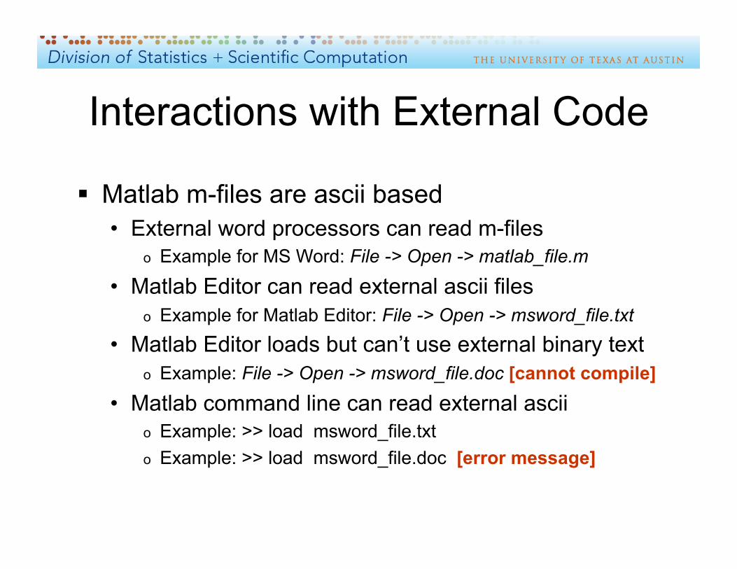
Interactions with External Code

Matlab m-files are ascii based • External word processors can read m-files

o Example for MS Word: File -> Open -> matlab_file.m

• Matlab Editor can read external ascii files o Example for Matlab Editor: File -> Open -> msword_file.txt

• Matlab Editor loads but can’t use external binary text o Example: File -> Open -> msword_file.doc [cannot compile]

• Matlab command line can read external ascii o Example: >> load msword_file.txt o Example: >> load msword_file.doc [error message]

Thanks for Coming!

Please complete course evaluation: • https://www.surveymonkey.com/s/LRJ6WJK

More free individual assistance available (e-mail or consulting appointment)

matlab-ii: computing, programming and data analysisylataus/matlab/matlabii.pdf · matlab-ii:...

Documents