MATLAB Primer

Dr. Robert L. Williams II Mechanical Engineering

Ohio University

© 2018 Dr. Bob Productions

williar4@ohio.edu www.ohio.edu/mechanical-faculty/williams

Adept 550 SCARA Robot MATLAB Simulation/Animation

This document is intended as a reference guide to help students learn MATLAB software for simulations and animations in kinematics, dynamics, controls, biomechanics, and robotics. The usefulness of this MATLAB Primer extends well beyond these fields.

2

Table of Contents

1. INTRODUCTION................................................................................................................................ 4 

2. BASICS ................................................................................................................................................. 5 

3. HELP ..................................................................................................................................................... 8 

4. RESERVED NAMES .......................................................................................................................... 9 

5. BASIC OPERATIONS AND FUNCTIONS .................................................................................... 10 

6. PRECISION ....................................................................................................................................... 12 

7. STRINGS ............................................................................................................................................ 13 

8. COMPLEX NUMBERS .................................................................................................................... 14 

9. ARRAYS ............................................................................................................................................. 15 

10. PLOTTING ...................................................................................................................................... 18 

11. NONLINEAR EQUATIONS SOLUTION .................................................................................... 23 

12. DIFFERENTIAL EQUATIONS SOLUTION .............................................................................. 24 

13. POLYNOMIALS ............................................................................................................................. 25 

14. VECTORS ........................................................................................................................................ 26 

15. MATRICES AND LINEAR ALGEBRA ....................................................................................... 27 

16. WORKSPACE DATA ARCHIVING ............................................................................................ 29 

17. USER INPUT ................................................................................................................................... 30 

18. PROGRAMMING ........................................................................................................................... 33 

19. FUNCTIONS .................................................................................................................................... 36 

20. EDITOR/DEBUGGER .................................................................................................................... 37 

21. M-FILES MANAGEMENT ............................................................................................................ 38 

22. TOOLBOXES .................................................................................................................................. 39 

23. SYMBOLIC MATH ........................................................................................................................ 40 

24. SIMULINK TUTORIAL ................................................................................................................ 41 

25. PITFALLS ........................................................................................................................................ 44 

26. SAMPLE M-FILES ......................................................................................................................... 50 

APPENDIX. INTERACTIVE PLOT TOOLS .................................................................................... 54 

3

MATLAB Primer

Dr. Bob Williams williar4@ohio.edu

Ohio University The purpose of this primer is to familiarize the student with MATLAB software in engineering design, analysis, and simulation. MATLAB is used extensively in all of my required and elective undergraduate and graduate engineering courses at Ohio University. My primary teaching and research interests are kinematics, dynamics, controls, haptics, biomechanics, and robotics, so I would not be surprised if this primer favors those areas. However, MATLAB is very general, with many toolboxes and specific functions for many engineering, technical, and scientific fields. This primer is intended to be a good introduction and reference for all students interested in applying the power of MATLAB to their engineering problems. This primer presents the following MATLAB topics: introduction, basics, help, reserved names, basic operations and functions, precision, strings, arrays, plotting, nonlinear equations solvers, differential equations solvers, polynomials, vectors, matrices and linear algebra, workspace data archiving, programming, functions, the editor/debugger, m-files management, toolboxes, potential pitfalls, and sample m-files.

MATLAB stands for MATrix LABoratory. In this primer bold Courier New font indicates MATLAB function names, user inputs, variable names, and MATLAB outputs; this is given for emphasis only.

Since MATLAB is relatively expensive software and since Mathworks seems to be getting more

and more like Microsoft as time goes by, one may want to check out FreeMat: freemat.sourceforge.net. Currently this FreeMat does not include a lot of the commands covered in this MATLAB Primer, especially the graphical and user-interface commands.

See Dr. Bob’s Atlas of Structures, Mechanisms, and Robots for an extensive gallery of MATLAB

Simulations/Animations developed by Dr. Bob at Ohio University to support specific courses:

www.ohio.edu/mechanical-faculty/williams/html/PDF/MechanismAtlas.pdf

4

1. Introduction MATLAB is a general engineering analysis and simulation software. It was originally developed specifically for control systems simulation and design engineering, but it has grown over the years to cover many engineering and scientific fields. MATLAB is based on the C language, and its programming is vaguely C-like, but simpler. MATLAB is sold by Mathworks Inc. (www.mathworks.com). Ohio University has a limited site license and all students are encouraged to buy the student version of MATLAB for installing on their personal computers (versions are available for the major computer platforms and operating systems). The student version is basically the same as the full professional version, with artificial limits on variables such as limiting maximum matrix size. Additionally, the student version includes all toolboxes, many of which must be purchased separately in the professional version. When Dr. Bob worked at NASA Langley Research Center in the late 1980s and early 1990s we sponsored a fledgling company called Mathworks to develop a controls engineering software that grew into MATLAB. We were able to evaluate and use early beta versions, providing feedback for early MATLAB development. Dr. Bob was one of the first, if not the first, to bring MATLAB software to Ohio University for engineering education and research. Mathworks Inc. has developed the MATLAB Onramp, a free, on-line, self-paced course for beginners that is advertised to last about 2 hours (need not be contiguous):

matlabacademy.mathworks.com

5

2. Basics

To start the MATLAB software in the Windows or Mac environment simply double-click on the MATLAB icon. Upon initiation of the MATLAB software my MATLAB window displays:

To get started, select MATLAB Help or Demos from the Help

menu. >>

The >> symbol is the MATLAB command prompt, where the user can type inputs to MATLAB.

MATLAB provides several windows in the initial interface (Command Window, Command History, File Search Path) – I generally X out most of these with the mouse and just use the Command Window (and the MATLAB Editor/Debugger – described later).

MATLAB is case-sensitive, which means that variables a and A are different. At the command prompt >> MATLAB can be used like a calculator. Press <Enter> to see a

result or semi-colon (;) followed by <Enter> to suppress a result. >> 2+3 ans = 5 >> 2*3 ans = 6 >> 2-3 ans = -1 >> 2/3 ans = 0.6667 >> sqrt(9) ans = 3 >> 4^2 ans = 16 >> a = 4; b = 6; a+b ans = 10

6

% The % symbol at any point in the code indicates a comment; text beyond the % is ignored by MATLAB and is highlighted in green. This primer will henceforth use this notation for explanations.

; % The semicolon is used at the end of a line suppresses display of the line’s result

to the MATLAB workspace. It is also used to separate rows in entering arrays, vectors, and matrices.

clear % This command clears the MATLAB workspace, i.e., erases any previous user-

defined variables. clc % Clear the MATLAB Command Window and move the cursor to the top. ... % Continue statement to the next line. who % Displays a list of all user-created variable names. whos % Same as who but additionally gives the dimension of each variable.

MATLAB is interpretive like the Basic programming language, that is, it executes line by line

without the need for a compiler. MATLAB commands and functions can be typed right into the MATLAB command window – this gets old fast, especially with complicated statements. Therefore, the recommended mode to execute MATLAB statements is to develop m-files containing your desired program to execute. Put your sequence of MATLAB statements in an ASCII file name.m, created with the beautiful MATLAB Editor/Debugger – this is color-coordinated, tab-friendly, with parentheses alignment help and debugging capabilities.

To run an existing m-file name.m, type the filename name in the MATLAB command window,

making sure that the m-file exists in the MATLAB file search path. DO NOT type name.m, only name. As an alternative, click the save-and-run button in the MATLAB editor to run the m-file. Using this method, if the m-file is not within the MATLAB search path, it automatically offers to add your current folder location to the search path. To set the MATLAB working directory to one that you have used before, click the down-arrow up at the top of the MATLAB window – the text box displays the current working directory and the list shows recently-used directory choices. To browse for new folders not on this list and set one as the current working directory, use the … button directly to the right of the working directory down-arrow.

To halt an m-file prematurely (e.g. to stop execution of an unintended infinite loop), press ctrl-

c. If you use the ; suppression discussed earlier, the variable name(s) still hold the resulting value(s)

– just type the variable name at the command prompt after the program runs to see the value(s). If there is a syntax or programming logic error, it will give an error message at the bad line and then quit. Even though there is no compiler, MATLAB can recognize certain errors up-front and refuse to execute until those errors are corrected. For other errors, the program will execute until reaching the bad line. Error messages in MATLAB are generally very specific and helpful, sometimes including the precise m-file line and column number where the error occurs.

7

The up-arrow recalls previously-typed MATLAB commands at the MATLAB prompt, in reverse

order (most recent first). The down-arrow similar scrolls forward through previously-typed MATLAB commands.

Almost all of my m-files start with the following line (multiple commands may appear on the same

line, separated by space(s) and/or a semi-colon): clear; clc;

(Exception – if I want to use the results of one m-file in another m-file executed after the first, I omit clear so those results will not be erased..)

I have found that MATLAB is generally very reliable in terms of changes between software versions, i.e. old m-files can be run reliably using newer versions. If MATLAB plans to obsolete a function or command they prepare you for this with informational messages when using those commands. To determine the MATLAB software version number you are running type version:

>> version ans = 7.3.0.267 (R2006b)

This primer was developed mainly using the R2006b version – it should be largely compatible with the future MATLAB versions.

8

3. Help After initiating the MATLAB software, a good way to start learning is to click on MATLAB Help and/or Demos. Alternatively, one may type MATLAB Help and/or Demos at any time from the MATLAB prompt >>. On-line MATLAB help is generally very useful. If you are really lost type help to learn how to use the MATLAB help facility.

help % Provides a list of topics for which you can get online help, sorted in logical groups. Click on any topics to see the applicable MATLAB functions.

help fname % Provides online help for MATLAB function fname (see help for

function names). The help fname command prints the header of the m-file help.m. That is, MATLAB includes comments at the top of each m-file to explain what each function or command does, how to use it, and the input/output requirements (usually there are several I/O options). MATLAB m-files are viewable by the user if you look in the MATLAB install folder. But you needn’t look inside any m-files, the help command prints the header to the command window to explain the function.

Related functions of interest are generally suggested when using help fname, at the end of the help text (See also . . .). This is a good way to find other related functions that you will want to learn and use. If you don’t know the specific MATLAB function name but only the general topic, use:

lookfor topic % Provides a list of functions for which you can get online help, related to your search topic.

For instance, lookfor matrices responds with a host of available functions for matrices and linear algebra. Here are some more help-related functions: info % Provides contact info for Mathworks Inc., who makes MATLAB. whatsnew % Highlights changes from the previous MATLAB versions.

9

4. Reserved names The following variable names are reserved for specific standard reasons by MATLAB. All can be overwritten, i.e. re-defined using the = assignment, but this is to be avoided (except when using i and j for loop counters). pi % 3.1415926535897.... = 4*atan(1) inf % infinity NaN % Not a Number, such as 0 / 0 or inf-inf i % sqrt(-1) j % sqrt(-1) eps % machine precision, 2.2204e-016 on my computer

ans % answer: the result of a MATLAB operation when no name is assigned (ans is constantly overwritten with the latest non-named operation)

flops % number of floating point operations (obsolete since MATLAB 6)

10

5. Basic Operations and Functions This section covers some basic MATLAB operations and built-in functions.

= % assignment of a calculation result to a variable name

+ % addition - % subtraction * % multiplication / % division \ % left division ^ % exponentiation sin cos tan cot sec csc % trigonometric functions asin acos atan acot asec acsc % inverse trigonometric functions atan2(num,den) % quadrant-specific inverse tangent sinh cosh tanh coth sech csch % hyperbolic trig functions asinh acosh atanh acoth asech acsch % inverse hyperbolic trig functions sind cosd tand cotd secd cscd % trigonometric functions in degrees asind acosd atand acotd asecd acscd % inverse trig functions in degrees exp % exponential function, base e log % natural logarithm log2 % base 2 logarithm log10 % base 10 logarithm sqrt % square root

11

abs % absolute value sign % signum function (returns +1 for positive, 0 for zero, –1 for negative) rand % random number or array generator randn % random number or array generator with normal distribution factorial % factorial function

Most operations and functions in MATLAB are overloaded, i.e. they work appropriately differently when the same function (operator) is presented with different input data types; e.g. scalars, vectors, and matrices can all be added or subtracted. These data types can also be multiplied, but only if the indices line up correctly for matrix multiplication. Order of Operations. MATLAB follows the standard precedence of mathematical operations you are already familiar with, i.e. from first to last priority:

1. parentheses 2. exponentials 3. multiplication and division 4. addition and subtraction

For equal precedence operations, the calculation proceeds left-to-right. Then function evaluations are last (nested from within first if there are functions of functions). That is, you can place any computations within a function call and MATLAB will evaluate the computations first and then call the function evaluation with the result. For example:

>> x = 1; y = 2; z = 3; >> cos(x^2 + (2*y - z)) ans = -0.4161

Since x^2 + (2*y - z) first yields 2.

12

6. Precision All MATLAB numerical computations are performed in double precision by default, but the user can enter the following commands to control the numerical display format. As presented earlier, eps is the reserved MATLAB name for machine precision. format short % 4 decimals format long % 14 decimals format short e % scientific notation with 4 decimals format long e % scientific notation with 15 decimals format rat % ratio of integers approximation format hex % hexadecimal format There are many other format options one can learn by entering help format. Here are the MATLAB variable types (The FreeMat Primer, G. Schafer):

int8 signed 8 bit integer, –128 to 127 int16 signed 16 bit integer, –32,768 to 32,767 int32 signed 32 bit integer, –2,147,483,648 to 2,147,483,647 int64 signed 64 bit integer, -9,223,372,036,854,775,808 to 9,223,372,036,854,775,807 uint8 unsigned 8 bit integer, 0 to 255 uint16 unsigned 16 bit integer, 0 to 65,535 uint32 unsigned 32 bit integer, 0 to 4,294,967,295 uint64 unsigned 64 bit integer, 0 to 1.844674407370955e+019 float signed 32 bit floating point number, -3.4 x 1038 to 3.4 x 1038 (single precision) double signed 64 bit floating point number, -1.79 x 10308 to 1.79 x 10308 complex signed 32 bit complex floating point number (real and imaginary parts are single) dcomplex signed 64 bit complex floating point number (real and imaginary parts are double) string letters, numbers, and/or special characters, up to 65535 characters long

13

7. Strings Like most programming languages MATLAB can define and display text strings: s = 'Place text here.' % create a MATLAB string A string is a vector whose components are the numeric codes for the ASCII characters. The length and size functions (see the section on Arrays) also work for strings, giving the number of characters. An apostrophe within a string is indicated by two apostrophes. disp(s) % print the string s to the screen disp('text') % print the string text to the screen error('Error message here.') % display an error message warning('Warning message here.') % display a warning message

strcmp % compare strings – returns 1 for identical and 0 otherwise

For string formatting, MATLAB uses LaTex notation, as in the following examples: Greek characters: \theta gives lower-case and \Theta gives upper-case You can use the entire Greek alphabet, both lowercase and capitals. Font formatting: \it gives italics, \bf gives bold type, and \fontname changes the font type \fontsize changes the font size _{text} makes a subscript and ^{text} makes a superscript You can combine any of these formatting methods in any one text string. Use the curly brackets { } to delineate formatting – they will not appear in the text. A later section on Plotting includes more information on text strings to annotate plots.

14

8. Complex Numbers MATLAB uses both i and j to represent the imaginary complex operator 1 . Caution: both i and j (as well as any other reserved names) can be re-defined, and these two often are, such as using i and j for loop iteration variables. To enter a complex number in MATLAB: c = 8 + 3*i; % enter a complex number c = 8 + 3*j; % enter a complex number c = complex(8,3); % enter the same complex number, alternative Here are some useful MATLAB functions for complex numbers: d = conj(c); % define the complex conjugate of a complex number

real(c) % returns the real part of a complex number imag(c) % returns the imaginary part of a complex number abs(c) % returns the magnitude of a complex number angle(c) % returns the direction of a complex number isreal(c) % returns 1 if the number is complex, 0 otherwise

15

9. Arrays Arrays are m x n dimensional collections of numbers. MATLAB also allows 3D arrays. Scalars are 0-dimensional arrays, vectors are 1-dimensional arrays, matrices are 2-dimensional arrays, and a collection of matrices are 3-dimensional arrays. To establish an equally-spaced 1D array, use: t = [t0:dt:tf]; % equally-spaced time array where t0 is the initial time, dt is the time step, and tf is the final time. These numerical values should be set such that there is an integer number of time values N, i.e.:

0 1ft tN

dt

For example, t = [0:0.1:1]; yields the array [0 0.1 0.2 … 1]. One can include a null element if desired, e.g. t(2) = [ ];. If you don’t want to determine a nice dt to yield an integer N, use: t = linspace(t0,tf,N-1); % equally-spaced time array, alternate Two useful functions to automatically determine the array dimensions are size and length:

>> size(t) ans = 1 11 >> length(t) ans = 11

To obtain an element of an array, use the (i) notation. For example:

>> t(3) ans = 0.2000

To obtain a contiguous subset of an array, use the (i:j) notation. For example:

>> t(3:7) ans = 0.2000 0.3000 0.4000 0.5000 0.6000

Most functions can accept arrays as inputs, for example cos(t). However, the multiply (*) and square (^2) operators will not work with arrays since matrix multiplication is impossible with (1xn)(1xn) dimensions:

16

>> t(3:7)^2 ??? Error using ==> ^ Matrix must be square.

If you want to perform element-by-element operations on arrays, use the dot notation:

>> t(3:7).^2 ans = 0.0400 0.0900 0.1600 0.2500 0.3600

The dot notation also works with element-by-element multiplication and division: .^ % array element-by-element exponentiation .* % array element-by-element multiplication ./ % array element-by-element division .\ % array element-by-element left division The following functions apply to statistical array calculations: max, min, mean, median, std, sort, sum, diff, prod Finding the array index i at which the maximum Ymax and minimum Ymin values occur is done as follows, for a given array Y: [Ymax,i] = max(Y); [Ymin,i] = min(Y);

17

It is convenient to use the array power of MATLAB in programming (see the section on Programming). For example, here are two ways to define the identical time array:

1. dt = 0.1; for i = 1:11, t(i) = (i-1)*dt; end 2. t = [0:0.1:1];

Both yield the array t = [0 0.1 0.2 … 1]. Then here are two alternative ways to perform a function calculation for all array values:

1. for j = 1:11, f(j) = cos(t(j)); end 2. f = cos(t);

Both methods yield the same array f, the cosine of all t values. Clearly method 2 is preferable in both cases for brevity and readability.

MATLAB function meshgrid generates arrays from two or three vectors (see Section 14) for use in 3D function evaluation, 3D plotting, and other applications.

[X,Y] = meshgrid(x,y); % Transforms the domain specified by vectors x and y into arrays X and Y that can be used for the evaluation of functions of two variables and 3D surface plots. The rows of the output array X are copies of the vector x and the columns of the output array Y are copies of the vector y.

[X,Y] = meshgrid(x); % Same as [X,Y] = meshgrid(x,x);

[X,Y,Z] = meshgrid(x,y,z); % Extension of [X,Y] = meshgrid(x,y).

Produces 3D arrays XYZ that can be used to evaluate functions of three variables xyz and also 3D volumetric plots.

18

10. Plotting Generating 2D plots in MATLAB is easy: plot(x,y); % plot dependent variable y versus independent variable x Where y is plotted on the ordinate axis and x is plotted on the abscissa axis. x and y must both be arrays of equal sizes (1 x n or n x 1). To plot multiple curves on the same graph: plot(x,y1,x,y2,x,y3); To distinguish between the curves one may use different colors, linetypes, markers, or combinations of these. The default colors are:

yellow (y), magenta (m), cyan (c), red (r), green (g), blue (b), white (w), black (k) The possible linetypes are:

solid (-) dashed (--) dotted (:) dashed-dot (-.) The possible markers are:

point (.) plus (+) star (*) circle (o) ex (x) down triangle (v) up triangle (^) left triangle (<) right triangle (>) square (s) diamond (d) pentagram (p) hexagram (h)

We can combine curve characteristics. For example: plot(x,y1,’r--’,x,y2,’g:’,x,y3,’b-.’); To plot a sine and cosine function on the same graph is straight-forward (see the first plot below):

ph = [0:5:360]; y1 = cosd(ph); y2 = sind(ph); figure; plot(ph,y1,ph,y2);

To plot a more professional graph requires bigger font, a title, axis labels and units, a grid, a legend, controlled color and linetypes, and controlled axis limits (see the second, improved plot below):

figure; plot(ph,y1,'r--',ph,y2,'g:'); grid; axis([0 360 -1 1]); set(gca,'FontSize',18); xlabel('{\it\phi} ({\itdeg})'); ylabel('{\itf(\phi)} ({\itunitless})'); legend('{\itcos}', '{\itsin}'); title('Trigonometric Plots');

The plot legend may be dragged to a more convenient location with the mouse, to avoid covering plots.

19

Trig Plots

Improved Trig Plots

0 50 100 150 200 250 300 350 400-1

-0.8

-0.6

-0.4

-0.2

0

0.2

0.4

0.6

0.8

1

0 50 100 150 200 250 300 350-1

-0.8

-0.6

-0.4

-0.2

0

0.2

0.4

0.6

0.8

1

(deg)

f()

(un

itles

s)

Trigonometic Plots

cossin

20

Here are some general plot commands: figure; % creates an empty figure window for graphics clf; % clear current figure

close all; % close all open figure windows – this is useful if your m-file generates a lot of plots, enter this command prior to running the program again.

fplot; % plot user-defined function

text(x,y,'string'); % position the text string at x,y in the current graphics window

gtext('string'); % position text string interactively in current

graphics window [x,y] = ginput; % collect graphical input from mouse in x and y

arrays. Press <Enter> to quit collecting hold; % hold current graph – hold on and hold off

to release axis('square'); % specify square axes axis([xmin xmax ymin ymax]); % specify axis limits axis('equal'); % specify axes with equal x and y ranges

axis('tight'); % set plot window to perfectly cover the entire x and y ranges, showing all data but no more

Here are some other 2D plot options:

polar, bar, hist, loglog, semilogx, semilogy To draw lines, again use plot(x,y); where x and y are now arrays containing the endpoint of the line to draw. For example: x = [0 L*cos(th)]; y = [0 L*sin(th)]; The above will draw a single rotating link of length L at a snapshot with angle th. This single link can be animated by incrementing th and plotting the line within a for loop (see MATEx2.m). The animation will zip right by without seeing it unless you use pause(dt); where dt is the pause time in seconds (approximately real-time).

21

I do a lot of MATLAB animations for visualizing the simulated motion of various mechanisms and robots, both planar and spatial. The default line width is marginal for representing real-world mechanical devices so I use the 'LineWidth' switch in the plot command as follows (the default thin width is 1 and I have used up to 5 for thick lines): plot(x,y,'g','LineWidth',3); % draw a green link with a thicker line width To draw solid polygons, use: patch(x,y); where x and y are now arrays containing the vertex coordinates of the polygon. Note you needn’t go back to vertex 1, but MATLAB closes the polygon for you. For example: x = [x1 x2 x3 ... xn]; y = [y1 y2 y3 ... yn]; 3D plots in MATLAB are similar to 2D plots: plot3(x,y,z); % 3D plot x vs. y vs. z Where x, y, and z must all be arrays of equal sizes (1 x n or n x 1). Again, one can plot multiple curves on the same graph. To control the viewing angle via azimuth az and elevation el: view(az,el); Here are some other 3D plot options:

surf, contour3, cylinder, sphere, peaks (MATLAB logo) Plots may be saved in name.fig format via the menus on each figure window:

File Save As... name.fig can then be retrieved later using the MATLAB open file icon or

File Open... Plots may be copied to the clipboard for other Windows applications via the menus on each figure window:

Edit Copy Figure First, if necessary, one can change the options via the same menu (the default works well):

Edit Copy Options...

22

After generating a plot there are many useful annotations and editing capabilities available via mouse interaction with the figure menus. I don’t tend to use these a lot since I would rather do the same functions in automated m-files which I can re-use for ensuing projects. See the Appendix for a description of interactive MATLAB plot tools. One can generate a grid of plots using MATLAB function subplot:

subplot(mni) will generate the ith plot in an m x n array of plots in the same figure window. Here is a specific example for a 2 x 2 subplot arrangement. Note that any useful plot annotation commands can still be used, plot by plot, with a subplot approach. figure; subplot(221) plot(t,x1); grid; set(gca,'FontSize',18); ylabel('\itx_1 (m)'); subplot(222) plot(t,x2); grid; set(gca,'FontSize',18); ylabel('\itx_2 (m)'); subplot(223) plot(t,x3); grid; set(gca,'FontSize',18); ylabel('\itx_3 (m/s)'); xlabel('\ittime (\itsec)'); ; subplot(224) plot(t,x4); grid; set(gca,'FontSize',18); ylabel('\itx_4 (m/s)'); xlabel('\ittime (\itsec)'); ; No spaces or commas are necessary in the subplot(mni) command, though these can be used if desired. The subplots will be filled in row-wise, i.e. the upper-left, upper-right, lower-left, and lower-right locations correspond to the (221), (222), (223), and (224) designations, respectively. In this example these further correspond to the x1, x2, x3, and x4 variables, respectively. The following code structure and functions may be used to save your MATLAB animation to an AVI movie file that can be played later independently of MATLAB (see the Programming chapter and also MatEx2.m).

for i=1:N, plot(...); Moov(i) = getframe;

end movie2avi(Moov,'Name.avi')

23

11. Nonlinear Equations Solution MATLAB has functions for solving systems of non-linear algebraic equations. Here are a few common ones:

fzero % numeric solution of a nonlinear algebraic equation in one variable fminsearch % numeric solution of nonlinear algebraic equations in multiple variables solve % symbolic solution of nonlinear algebraic equations

24

12. Differential Equations Solution MATLAB has many functions for solving differential equations. Here are a few common ones:

ode23 % 2nd-3rd order Runge-Kutta numerical solution ode45 % 4th-5th order Runge-Kutta numerical solution dsolve % symbolic solution for differential equations impulse % numerical differential equation solution for an impulse input (t) step % numerical differential equation solution for a unit step input lsim % numerical differential equation solution for any input

MATLAB can perform numerical (or symbolic) differentiation and integration:

diff % numerical difference and approximate derivative or symbolic derivative

quad % numerical integration

dblquad % numerical double integration

triplequad % numerical triple integration

int % symbolic integration

25

13. Polynomials A general polynomial has the form:

1 21 2 1 0

n nn na s a s a s a s a

Here the independent variable is s, the Laplace frequency variable, but the independent variable could be t, x, or anything you want, MATLAB doesn’t care. To define a polynomial in MATLAB enter an array with the n+1 numerical polynomial coefficients, in descending order of s-powers:

GenPoly = [an anm1 . . . a2 a1 a0]; % enter a general polynomial via its coefficients

Here is a specific example for a 4th-order polynomial (n = 4): 4 3 210 35 50 24s s s s

Poly4th = [1 10 35 50 24]; % enter a 4th-order polynomial via its coefficients To find the roots of a polynomial:

PolyRoots = roots(GenPoly) % to find the roots of a polynomial

>> roots(Poly4th) ans = -4.0000 -3.0000 -2.0000 -1.0000

To generate a polynomial from its roots (which are contained in array PolyRoots):

poly(PolyRoots) % build a polynomial from its roots

>> bob = poly(ans) bob = 1.0000 10.0000 35.0000 50.0000 24.0000

Here are some other useful polynomial functions:

conv % multiply factors to obtain a polynomial product deconv % divide a polynomial by specified factors to obtain a polynomial quotient;

synthetic division with remainder polyval % evaluate a polynomial numerically for an independent variable array polyfit % best polynomial fit to numerical data polyder % polynomial derivative

26

14. Vectors Vectors are 1-dimensional arrays. To enter vectors use:

v1 = [1 2 3]; % enter a 1x3 row vector v2 = [1;2;3]; % enter a 3x1 column vector

To separate elements on a row use spaces (or commas); to separate elements in a column use a semi-colon. Vector addition or subtraction is simply accomplished using the standard + and – operators. To obtain an element of a vector, use the (i) notation. For example:

>> v1(3) ans = 3.0000

To obtain a contiguous subset of a vector, use the (i:j) notation. For example:

>> v2(2:3) ans = 2.0000 3.0000

The following are useful vector functions:

dot(a,b) % vector dot product

cross(a,b) % vector cross product

transpose(a) % transpose of a vector

a’ % transpose of a vector, shorthand notation

norm(a) % length (Euclidean norm) of a vector [th,r] = cart2pol(x,y); % convert Cartesian to polar vector description [x,y] = pol2cart(th,r); % convert polar to Cartesian vector description [th,phi,r] = cart2sph(x,y,z); % convert Cartesian to 3D spherical description [x,y,z] = sph2cart(th,phi,r); % convert 3D spherical to Cartesian description The dot product is applicable to any equal-sized vectors and is identical to a’*b. The vector cross product is only applicable to 3x1 (or 1x3) vectors; planar vectors need a zero z component. The size and length functions introduced earlier under arrays apply to vectors.

27

15. Matrices and Linear Algebra Matrices are 2-dimensional arrays. To enter matrices use:

A = [1 2 3 4;5 6 7 8; 9 10 11 12]; % enter a 3x4 matrix A = [1 2 3 4; % enter a 3x4 matrix, alternate 5 6 7 8; 9 10 11 12];

Clearly the second method to enter the same matrix is more readable. To separate elements on a row use spaces (or commas); to separate rows from each other use a semi-colon. Matrix addition or subtraction is simply accomplished using the standard + and – operators. Matrix multiplication with appropriate dimensions is accomplished using the standard * operator. To obtain an element of a matrix, use the (i,j) notation, where i refers to the row index and j the column index. For example:

>> A(2,3) ans = 7.0000

To obtain a contiguous subset of a matrix, use the (i:j,k:l) notation. For example:

>> A(1:2,2:3) ans = 2.0000 3.0000 6.0000 7.0000

To obtain an entire row i of a matrix, use the (i,:) notation. That is, if the indices are omitted with the : notation, MATLAB just assumes you want the entire column range. For example:

>> A(2,:) ans = 5.0000 6.0000 7.0000 8.0000

To obtain an entire column j of a matrix, use the (:,j) notation. That is, if the indices are omitted with the : notation, MATLAB just assumes you want the entire row range. For example:

>> A(:,3) ans = 3.0000 7.0000 11.0000

28

The following are matrix functions: eye(n) % create an n x n identity matrix In zeros(m,n) % create a m x n matrix of zeros ones(m,n) % create a m x n matrix of ones

diag(v) % create a diagonal matrix with vector v on the diagonal diag(A) % extracts the a diagonal terms of matrix A into a vector

transpose(A) % transpose of matrix A

A’ % transpose of matrix A, shorthand notation

inv(A) % inverse of matrix A

pinv(A) % pseudoinverse of matrix A x = A\b; % Gaussian elimination to solve A x = b

eig(A) % find the eigenvalues of A [v,d] = eig(A) % find the eigenvectors and eigenvalues of A rank(A) % calculate the rank of matrix A det(A) % calculate the determinant of square matrix A norm(A) % return the norm of matrix A, many options cond(A) % return the condition number of matrix A trace(A) % calculate the trace of matrix A

The size and length functions introduced earlier under arrays and vectors also apply to matrices. MATLAB allows 3D arrays, i.e. sets of matrices. This feature is very useful in robotics, where the pose (position and orientation) of one Cartesian frame with respect to another is represented by 4x4 homogeneous transformation matrices. In a given robot there are many of these 4x4 matrices to describe the pose of all joints/links within the robot.

29

16. Workspace Data Archiving One can save and recall the MATLAB workspace. That is, variables that you created and manipulated in one MATLAB session can be saved for later recall and future work.

save % saves all user-created variables in the binary file matlab.mat

save filename % saves all user-created variables in the binary file

filename.mat save filename x y z % saves the user-created variables x, y, and z in the binary

file filename.mat There are many options for data formatting – enter help save to learn these. To recall MATLAB data saved earlier using the above commands, use:

load % loads all user-created variables from the binary file matlab.mat

load filename % loads all user-created variables from the binary file

filename.mat load filename x y z % loads the user-created variables x, y, and z from the

binary file filename.mat To save all the text that transpires in the command window during a MATLAB session, both input and output, use:

diary filename % copy all command window input and output to the file

filename. diary off % suspend copying the command window input and output. diary on % resume copying the command window input and output.

For MATLAB to write/read data files for Excel and other external programs, use:

csvwrite / csvread % write / read a comma-separated data file dlmwrite / dlmread % write / read an ASCII-delimited data file

30

17. User Input For user input data typed from the keyboard and choices from the mouse, use the input, menu, inputdlg, and ginput commands:

name = input('string') % The input command displays a text message string to the user,

prompting for input; the data entered from the keyboard are then written to the variable name. This data can be a scalar, vector, matrix, or string as the programmer desires.

Example:

R = input('Enter [r1 r2 r3 r4] (length units): '); r1 = R(1); r2 = R(2); r3 = R(3); r4 = R(4);

Upon execution, for example the user can type the following in the MATLAB command window in response to the prompt:

Enter [r1 r2 r3 r4] (length units): [10 20 30 40] and press the Enter key in order to ensure that MATLAB assigns:

r1 = 10 r2 = 20 r3 = 30 r4 = 40

var = menu('Message','Choice1','Choice2','Choice3',...) % The menu command displays a window on the screen, with the text

Message prompting the user to click their choice. Here the programmer types desired text in Choicei, which is written to the screen menu. Then the result of the user’s clicking is written as integer 1, 2, 3, … into the variable var, which can then be used for ensuing logical programming.

Example: choose = menu('What is your desire, master?','Snapshot','Moving'); will display the following menu on the screen for the user to click one choice with the mouse:

31

When the user clicks Snapshot, the variable choose is assigned the value 1 (causing the program to execute the Snapshot code, not shown), and when the user clicks Moving, the logical variable choose is assigned the value 2 (causing the program to execute the Moving animation code, not shown).

The MATLAB inputdlg command (input dialog) is very useful for convenient user data entry into a program, with built-in default values. Example: name = 'Input'; values = {'a','b','c'}; default = {'1.0','2.0','3.0'}; vars = inputdlg(values,name,1,default); a = str2num(vars{1}); b = str2num(vars{2}); c = str2num(vars{3}); This MATLAB code will display the following dialog box on the screen for the user to click with the mouse and enter data as desired, clicking OK to proceed in the program when finished entering data. If the default values are acceptable, the user need only click OK to proceed.

Note that strings are used in the above code to enter the name, values, and default values. This is why the str2num function is required, to convert strings to numerical values MATLAB can compute with. As such, it is critical to use the curly brackets { } as shown and not square brackets nor parentheses in their place.

32

The MATLAB ginput command is very useful for convenient user data entry into a program, via clicking the mouse in the current graphics window.

[X,Y,BUTTON] = ginput(N) % The ginput command allows the user to click in the current graphics

window and enter the data into the X, Y, and BUTTON arrays. X and Y are the coordinates chosen by the user’s mouse and BUTTON is 1, 2, or 3 for the left, middle, or right mouse buttons, respectively. N is the number of points to be collected and entered into the data arrays. If N is omitted, the user keeps clicking and saving points until the return key is pressed.

ginput example: %------------------------------------------------------------------------------ % Mousey.m % use ginput to get x,y,button data from the mouse in a graphics window % Dr. Bob 9/2014 in Puerto Rico %------------------------------------------------------------------------------ clear; clc; figure; axis('square'); axis([-10 10 -10 10]); grid; set(gca,'FontSize',18); xlabel('\itX (m)'); ylabel('\itY (m)'); N = 4; disp('Please choose the following number of points in the figure window: '); N [X,Y,BUTT] = ginput(N); % collect N XY data points via the mouse for i = 1:N, [X(i) Y(i) BUTT(i)] % print the N XY data points to the screen end

33

18. Programming This section discusses MATLAB programming. MATLAB programs are written using the MATLAB Editor/Debugger, saved in m-files, and executed by typing the filename at the MATLAB Command Window or by using the save-and-run button from the Editor. In either case, the m-file must reside on disk within the MATLAB file search path. MATLAB code is interpretive like the standard Basic programming language. That is, there is no compiling and statements are executed line-by-line in serial fashion. There is an optional compiler available to run MATLAB code more efficiently in standard C or C++ for real-time applications. Even though normal MATLAB is not compiled, a program may not run if MATLAB sees an error later in the m-file. MATLAB error statements (in red in the Command Window after attempted m-file execution) are usually very helpful, including a clear statement of the problem and the row and column numbers where the error occurs. MATLAB will only display one error at a time, either prior to execution or when the error is encountered during interpretive execution. Therefore, I usually must fix each error one at a time and then keep re-executing and re-fixing new errors until the entire program runs correctly. Always use good programming techniques, like with any programming language. Use appropriate tabs (in the MATALB editor, try right-click Smart Indent), and include generous line and character spacing to make the program more readable and logical. Use plenty of comments % with in-line or separate lines or blocks of comments. Often I will need to temporarily remove one or more lines of code to test various issues – in the MATALB editor, highlight the desired code line(s) and use right-click Comment (or Uncomment). Almost all of my m-files start with the commands:

clear; clc; to erase any previously-defined user-created MATLAB variables (clear) and to clear the screen and move the cursor to the top of the Command Window (clc).

34

Three useful programming constructs are the for loop, the while loop, and the if logical condition. These are familiar from other programming languages and the MATLAB syntax is: for i = 1:N, put loop statements here using (i) notation to pick off and save single array values end while (condition) put statements here to execute while condition is true end if (condition1) put statements here to execute for condition1 is true elseif (condition2) put statements here to execute for condition2 is true ... end N is the number of times to execute the for loop. Any number of elseif conditions may be included, or none at all. One can have nested loops and logical conditions in any program. Again, use right-click Smart Indent to make more readable m-file programs. In the while and if / elseif statements above, the condition and condition1 / condition2 can be compound conditions, i.e. using the Booleans below. The comparatives for the condition statements are standard: < % less than > % greater than <= % less than or equal to >= % greater than or equal to == % exactly equal to ~= % not equal to The Booleans in MATLAB again are standard: & % AND | % OR ~ % NOT

35

The following two commands are useful for halting execution until the user wants to resume: pause; % stop execution until the <Enter> key is pressed

waitforbuttonpress; % stop execution until a mouse button or keyboard key is pressed over a figure window

For instance, I routinely use:

if i==1 pause; % user presses <Enter> to continue end

inside a for loop when there is graphics and animation so that the user may see the initial mechanism or robot rendering, get acclimated to the view, and re-size the window prior to hitting <Enter> to continue the program and display the ensuing animation. Also, for animations, I use the following pause inside the for loop, otherwise the animation will zip right by without the user seeing anything:

pause(dt); % program pauses for dt seconds for animation purposes

This is approximately real-time and it unpauses automatically after dt has elapsed. In large, complicated programs I regularly use sub-m-files to simplify the programming. That is, I put a series of commands into a different m-file and then call it by typing the sub-m-file name in the calling m-file. This is not a subroutine or a function (see next section) but merely cutting lines which logically belong together, and which may need to be repeated, into a separate file. Then upon running the main program, the interpretive execution proceeds as if all commands were in the same file. Here are four program flow commands that I have never used in my life, but you may want to: break % stop execution of a for or while loop continue % go to the next iteration of a for or while loop keyboard % pause m-file execution for user keyboard input return % return to invoking function; also terminate keyboard mode For more advanced interactive applications, one may wish to create a GUI (graphical user interface). MATLAB has a very general and powerful GUI facility called GUIDE. To invoke it, either click the GUIDE button on the MATLAB toolbar, or simply type >>guide in the MATLAB command window. To get started with GUIDE, run the demo (Help Demos MATLAB Creating Graphical User Interfaces Creating a GUI with GUIDE).

36

19. Functions MATLAB comes with many useful built-in functions, many of which are covered in this primer. One can also write user-defined functions to perform specific calculations that you may need repeatedly. Here is an example user-created function to calculate the mobility M (number of degrees-of-freedom, dof) for planar jointed mechanical devices (structures, mechanisms, and robots), using Kutzbach’s planar mobility equation:

21213 JJNM

% Function for calculating planar mobility % Dr. Bob function M = dof(N,J1,J2) M = 3*(N-1) - 2*J1 - 1*J2;

Create the above function within the MATLAB editor and name it dof.m. Usage: mob = dof(4,4,0); % for 4-bar and slider-crank mechanisms Result: mob = 1 The command mob = dof(4,4,0); may be invoked either from MATLAB’s command window or from within another m-file. In either case, the file dof.m containing the function dof must be in the MATLAB file search path. For simple user-created functions, one can use inline: g = inline(‘x.^2 + 2*x + 3’,‘x’); % create an in-line function This yields the function 2( ) 2 3g x x x . To use it, simply enter g(4) and so on. Note that this function will work with scalar or array input due to our use of the .^ term-by-term exponentiation. The .* term-by-term multiplication is not required since the scalar multiplication of 2 works with arrays or scalars.

37

20. Editor/Debugger This section presents the MATLAB Editor/Debugger. In the MATLAB editor, comments % appear in green, text strings appear in violet, and logical operators and other reserved programming words such as looping words appear in blue. Errors in the command window appear in red. Press the new file button from the Command Window to invoke the MATLAB Editor/Debugger – a new window will open for you to enter your m-file. Be sure to Save As filename.m, in a folder that is in the MATLAB file search path. Alternatively, you may add the folder where you save the m-file to the search path. Use generous in-line and between-line spacing, and appropriate tabbing (right-click Smart Indent), to make the program more readable and logical. Use lots of comments %, at the end of lines and in separate lines and blocks of comments (right-click Comment or Uncomment). The MATLAB editor conveniently numbers the m-file lines consecutively from 1. The columns are not numbered, but if you place the cursor anywhere in the m-file using the mouse by single-clicking, the line and column numbers are displayed in the editor screen to the lower right (e.g. Ln 3 Col 15). There is a convenient button to save and run the m-file in the active editor window. Multiple m-files from different directories may be open simultaneously, even if two or more have the same filename. After running an m-file, place the cursor over different variables in the m-file inside the MATLAB Editor/Debugger to see the values. MATLAB has a powerful debugging capability within the Editor. Honestly I have not found the need to learn this so far. It is certainly recommended to the interested student, especially for more advanced programming. Debugging is critical when using functions extensively since their variables are not global. Use the profile on command to track the execution times of your m-file execution.

38

21. m-files management MATLAB uses a Unix-like directory structure and commands to access and manage m-files. pwd % show the current directory (folder) dir % list all files in the current directory dir *.m % list all m-files in the current directory dir *.mdl % list all Simulink models in the current directory chdir pathname % change the current directory to pathname chdir % show the current directory (just like pwd) cd % shorthand for chdir what % list all MATLAB files in the current directory which fname % displays the path name of the function fname.m. path % prints the current MATLAB file search path to the screen

addpath % add another directory to the current MATLAB file search path

rmpath % remove a directory from the current MATLAB file search path why % responds with funny answers – many possibilities

39

22. Toolboxes MATLAB has been expanded significantly over the years to include many fields besides control systems engineering, the initial MATLAB focus. Below is a partial list of available MATLAB toolboxes to expand the base MATLAB software capability. Ohio University does not have a license for all of these toolboxes. I especially recommend Simulink, the Control Systems Toolbox, Real-time Workshop, SimMechanics, the Symbolic Math Toolbox, and the Virtual Reality Toolbox.

Aerospace Blockset Aerospace Toolbox Communications Toolbox Control System Toolbox Curve Fitting Toolbox Data Acquisition Toolbox Filter Design Toolbox Financial Toolbox Fuzzy Logic Toolbox Genetic Algorithm Toolbox Image Processing Toolbox MATLAB Compiler Model Predictive Control Toolbox Neural Network Toolbox Optimization Toolbox Parallel Computing Toolbox Partial Differential Equation Toolbox Real-Time Workshop Robust Control Toolbox Signal Processing Toolbox SimBiology SimMechanics Simulink Simulink 3D Animation Simulink Control Design Simulink Design Optimization Spline Toolbox Stateflow Statistics Toolbox Symbolic Math Toolbox System Identification Toolbox Virtual Reality Toolbox

40

23. Symbolic Math As mentioned in the previous section, MATLAB provides a Symbolic Math Toolbox for performing symbolic analytical math operations, as opposed to numerical calculations. This is super useful in robotics and mechanisms derivations. Basically this can be useful in all branches of math, science, and engineering! A simple symbolic MATLAB m-file is given below for multiplying a matrix and a vector. Obviously, your instantiation of MATLAB must provide the Symbolic Toolbox in order to run this program. %---------------------------------------------- % % SymbEx.m % Example symbolic MATLAB program % Fall 2014, Dr. Bob in Puerto Rico % %---------------------------------------------- clear; clc; syms a b c d e f; % declare symbolic variables Matx = [a b;c d]; % define a 2x2 symbolic matrix Vect = [e; f]; % define a 2x1 symbolic vector Prod = Matx*Vect; % multiply the two symbolically pretty(Prod) % display the result The MATLAB output is as expected, requiring no numbers: [a e + b f] [ ] [c e + d f] Many, but not all, of MATLAB’s numerical functions are directly applicable to symbolic variables.

Even though this simple example does not require it, since Prod is already in the simplest possible form, one of the most useful Symbolic Math functions is:

simplify(SymbExpr); % simplify a symbolic expression This Symbolic Toolbox function automatically applies a hierarchy of trigonometric and algebraic simplification rules and identities in order to yield the simplest possible form for a symbolic expression. Funny results (but correct!) sometimes occur, and the human generally has to be involved, but I have seen some amazing simplifications generated automatically in this way.

41

24. Simulink Tutorial

Simulink is the Graphical User Interface (GUI) for MATLAB. This section presents a brief tutorial on how to use simulink to create an open-loop block diagram. Then the model can easily be run, i.e. asking simulink to numerically solve the associated IVP ODE for you and plot the results vs. time.

1. Start MATLAB and at the prompt type simulink (all lower case).

2. If installed, the Simulink Library Browser will soon pop up. 3. Click on the new icon, identical to a MS Word new file icon. That is your space to work in. After

creating a model it can be saved (using the save icon). 4. To build simulation models, you will be creating block diagrams just like we draw by hand. In

general all blocks are double-clickable to change the values within. In general you can connect the ports on each block via arrows easily via clicking and dragging with the mouse. You can also double-click any arrow (these are the controls variables) to label what it is. Same with all block labels (simulink will give a default name that you can change).

5. simulink uses EE lingo. Sources are inputs and sinks are outputs. If you click around in the

Simulink Library Browser, you will see the possible sources, blocks, and sinks you have at your disposal.

6. Now let us create a simple one-block transfer function and simulate it subject to a unit step input.

The given open-loop transfer function is 2

1( )

2 8G s

s s

.

a. Click the new icon in the Simulink Library Browser to get a window to work in (untitled

with the simulink logo).

b. Double-click the Continuous button in the Simulink Library Browser to see what blocks are provided for continuous control systems. Grab and slide the Transfer Fcn block to your workspace. Double-click the block in your workspace and enter [1] in Numerator coefficients and [1 2 8] in Denominator coefficients and close by clicking OK. Simulink will update the transfer function in the block, both mathematically and visually.

c. Go ahead and save your model on your flash drive as name.mdl (whatever name you

want, as long as it is not a reserved MATLAB word).

d. Click the Sources tab in the Simulink Library Browser to see what source blocks are provided. You will find a Step, Ramp, Sine Wave, etc. (but no Dirac Delta – see Dr. Bob’s on-line ME 3012 NotesBook Supplement to see how to make that type on input in Simulink, three alternate methods). Grab and slide the Step block to your workspace. Double-click the Step block in your workspace and ensure 1 is already entered as the final value (for a unit step) and that 0 is the Initial value. Close by clicking OK.

e. Draw an arrow from the Step block to the Transfer Fcn block by using the mouse. Float

the mouse near the Step port (> symbol) and you will get a large + mouse avatar. Click

42

and drag to the input port of the Transfer Fcn block; when you see a double-plus, let go and the arrow will be connected.

f. Click the Sinks tab in the Simulink Library Browser to see what sink blocks are provided.

Grab and slide the Scope block to your workspace.

g. Draw an arrow from the Transfer Fcn block to the Scope block by using the mouse, the same method as before.

h. To run the model (solve the associated differential equation numerically and plot the output

results vs. time automatically), simply push play (the solid black triangle button in your workspace window).

i. After it runs, double-click on your Scope to display the results. Click the binoculars icon

to zoom in automatically.

j. When I perform these steps, there are two immediate problems: i. the plot does not start until t = 1 sec and ii. the plot is too choppy. These are easy to fix:

i. Double-click the Step block and change the Start time to 0 from the default 1 sec,

then click OK. Re-run and ensure the plot now starts at t = 0.

ii. In your workspace window click Simulation -> Configuration Parameters -> Data Import/Export. Look for Refine output in the window and change the Refine factor from 1 to 10, then click OK. Re-run and ensure the plot is now acceptably smooth.

k. Finally in this open-loop simulation example, it appears that 10 sec final time is a bit too

much. Near the play button in your workspace is an unidentified number 10.0. This is the default final time. Change it to 8.0, re-run, and ensure the plot now ends at t = 8. If you reduce final time less than 8.0 you will lose some transient response detail.

Your final model will look like this (be sure to be a control freak like Dr. Bob and line up all the

arrows and blocks in a rectangular grid). I also renamed the blocks and labeled the variables.

Open-loop simulation example Simulink model

unit step time responseplot

1

s +2s+82

OL system

input u output y

43

Feel free to play around to your heart’s content and see what you can learn. Simulink is fast, easy, and fun! But it is a bad black box on top of the black box of MATLAB.

Another group of simulink blocks you may use a lot is under Math Operations in the Simulink Library Browser. In particular, we use the Sum (summing junction) and Gain (multiplication by a constant) a lot in controls.

In addition I find the Mux (multiplexer) and Demux (demultiplexer) very useful, especially the

Mux to combine two or more variables for plotting on a common scope. These are found under Signal Routing in the Simulink Library Browser.

Assignment: update your above model by yourself to include negative unity feedback (sensor

transfer H(s) = 1), with no specific controller (GC(s) = 1, just a straight line with no block). Plot both open- and closed-loop unit step responses and compare and discuss.

Hint: put a summing junction between the Step input and the OL system transfer function. Double-

click the sum to make the correct signs (i.e. + and -). Then pull an arrow down from the negative summing port, turn the corner without letting go. Then you will have to let go, but click immediately without moving the mouse and hover it over the output y line. When you get the double-plus, let go and you have just made a pickoff point, for the output y feedback.

44

25. Pitfalls This section contains some pitfalls that many MATLAB newbies encounter. Be sure to use proper m-file filenames. There can be no leading number, i.e. 4bar.m is an invalid filename in MATLAB, even though the MATLAB editor will let you name it as such. There can be no spaces in your filename, i.e. MATLAB will interpret the filename four bar.m as two separate text strings, even though Windows stupidly allows spaces in filenames. You can use the underbar instead of spaces and you can use numerical characters as long as they are not the leading character.

MATLAB is case-sensitive, which means that variables a and A are different. Also, generally MATLAB functions and commands are all lower-case. If you type a MATLAB command in all CAPS by mistake, such as WHOS instead of whos, this will fail – the MATLAB response is:

>> WHOS ??? Undefined function or variable 'WHOS'. However, if you want to run an m-file name.m and type in NAME in all capitals by mistake,

instead of name, MATLAB generally says the following and will run your m-file anyway:

Warning: Could not find an exact (case-sensitive) match for 'NAME'. MATLAB sample program MATEx2.m, given later, requires user-typed input from the keyboard to proceed: the = input('Enter [th0 dth thf] (deg): ') % User types input I created the text inside the input function – be sure to type the data in square brackets exactly as I specify in the text string above (without the(deg) which is for info only), and then hit <Enter>: Enter [th0 dth thf] (deg): [0 5 360] If you just cannot get the input function to work, skip it for now and just hard-code the data: th0 = 0; dth = 5; thf = 360; Be sure to comment out the input and following line in this case. If you are doing planar vector operations, the dot product will work:

>> a = [1;2]; b = [3;4]; >> dot(a,b) ans = 11

But the cross product will fail, until you augment the planar vectors with zero in the z component.

>> cross(a,b) ??? Error using ==> cross A and B must have at least one dimension of length 3.

45

>> a = [1;2;0]; b = [3;4;0]; >> cross(a,b) ans = 0 0 -2

Multiplying these two planar vectors will fail since the indices do not line up properly for matrix multiplication (2x1 times 2x1 and 3x1 times 3x1 will both fail since the inner matrix dimensions are not the same – for matrix multiplication, the number of columns in the left matrix must match the number of rows in the right matrix).

>> a*b ??? Error using ==> mtimes Inner matrix dimensions must agree.

Another way to perform the dot product is to transpose the first vector and use multiplication:

>> a'*b ans = 11

Now this matrix multiplication succeeds since the inner matrix dimensions match (1x3 times 3x1). A similar common error arises when an nx1 (or 1xn) array is squared:

>> b^2 ??? Error using ==> mpower Matrix must be square.

There are two potential fixes for this error. If you are inside an i loop and only intended to square one individual component, use the (i) notation:

>> b(2)^2 ans = 16

If you wanted to square each component of the original array and place the result in an equal-sized array, use the .^ element-by-element notation:

>> b.^2 ans = 9 16 0

When using the 2D plot command plot(x,y) both arrays x and y must be of the exact same dimension:

46

>> x = [0:1:10]; y = [2:2:20]; >> plot(x,y) ??? Error using ==> plot Vectors must be the same lengths.

To fix this case use whos to see the problem:

>> whos Name Size Bytes Class x 1x11 88 double y 1x10 80 double

We see that x is 1x11 and y is only 1x10. The same information could have been determined from length(x), length(y) (or size(x), size(y)). To fix this error:

>> x = [0:1:10]; y = [0:2:20]; >> plot(x,y)

Actually, the two arrays need not be of the exact same dimension – y of 1xn may be plotted vs. x of nx1 and vice versa. A common plotting error with newbies is when the user wants to plot an entire array vs. the independent variable array. By mistake, the user only plots a single scalar. In older versions of MATLAB this used to fail. Now MATLAB plots the following, barely visible:

>> c = 3; >> plot(x,c)

0 1 2 3 4 5 6 7 8 9 100

2

4

6

8

10

12

14

16

18

20

47

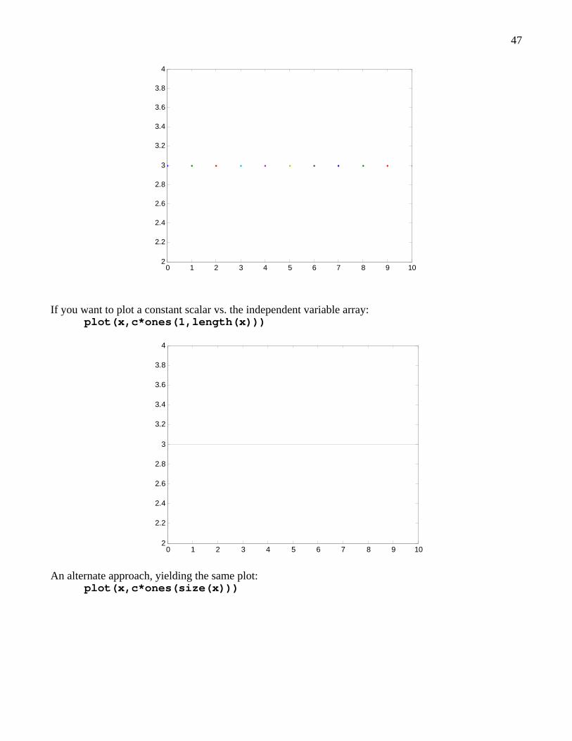
If you want to plot a constant scalar vs. the independent variable array:

plot(x,c*ones(1,length(x)))

An alternate approach, yielding the same plot:

plot(x,c*ones(size(x)))

0 1 2 3 4 5 6 7 8 9 102

2.2

2.4

2.6

2.8

3

3.2

3.4

3.6

3.8

4

0 1 2 3 4 5 6 7 8 9 102

2.2

2.4

2.6

2.8

3

3.2

3.4

3.6

3.8

4

48

Here are some more common errors I have seen with students and myself over the years. As in any programming, one must take care that your parentheses and brackets line up correctly, as you intended, and with proper left/right balancing:

>> sqrt(cos(t) ??? sqrt(cos(t) | Error: Expression or statement is incorrect--possibly unbalanced (, {, or [.

Whereas the C language starts indices at 0, and MATLAB is based on the C language, all MATLAB indices must start at 1:

>> b(0) = 10 ??? Subscript indices must either be real positive integers or logicals.

If you intended to define an array w2, but instead made a scalar w2, then if you try to access that variable w2 inside a loop for i greater than 1 you will get this error:

>> w2 = 5 >> w2(2) ??? Index exceeds matrix dimensions.

If you attempt to set a matrix equal to a left-hand-side array you will get this error:

>> b = rand(2); % generate a random 2x2 matrix b >> a(1) = b ??? In an assignment A(I) = B, the number of elements in B and I must be the same.

The fix for this error is to drop the (i) notation on the left-hand side. In general, if you are within a loop, only use the (i) notation on the left-hand side when you want to save that particular variable for later plotting or other operations. If the variable is intermediate and you don’t care about it, drop the (i) notation and then it will be overwritten the next time through the loop. If you intended to make an animation of robot or mechanism motion in a for loop of N steps but instead got N separate plot windows, you must move the figure; statement to outside the for loop. Then use close all; to kill the unwanted N figures on your screen prior to trying the program again. Remember to run an m-file name.m from the MATLAB command prompt, DO NOT type name.m, only name. Otherwise you will get the following error, since MATLAB thinks you are trying to access a data structure with .m in its name:

49

>> name.m ??? Undefined variable "name" or class "name.m".

50

26. Sample m-files The following example m-files are given on the following pages.

1) MATEx1.m matrix and vector definition, multiplication, transpose, and solution of linear equations

2) MATEx2.m input, programming, plots, animation 3) MATEx3.m complex numbers, polynomials, plotting

51%--------------------------------------------------------------- % MATLAB Example Program 1: MATEx1.m % Matrix and Vector examples % Dr. Bob, Ohio University %--------------------------------------------------------------- clear; clc; % clear any previously defined variables and the cursor % % Matrix and Vector definition, multiplication, and transpose % A1 = [1 2 3; ... % define 2x3 matrix [A1] (... is continuation line) 1 -1 1]; x1 = [1;2;3]; % define 3x1 vector {x1} v = A1*x1; % 2x1 vector {v} is the product of [A1] times {x1} A1T = A1'; % transpose of matrix [A1] vT = v'; % transpose of vector {v} % % Solution of linear equations Ax=b % A2 = [1 2 3; ...% define matrix [A2] to be a 3x3 coefficient matrix 1 -1 1; ... 8 2 10]; b = [3;2;1]; % define right-hand side vector of knowns {b} detA2 = det(A2); % first check to see if det(A) is near zero x2 = inv(A2)*b; % calculate {x2} to be the solution of Ax=b by inversion check = A2*x2; % check results z = b - check; % must be zero % % Display the user-created variables (who), with dimensions (whos) % who whos % % Display some of the results % v, x2, z % More vectors and matrices functions v1 = [1;2;3]; v2 = [3;2;1]; s3 = dot(v1,v2); v4 = cross(v1,v2); A = rand(3); v5 = A*v1; At = A'; Ainv = inv(A); i1 = A*Ainv; i2 = Ainv*A; dA = det(A);

52%--------------------------------------------------------------- % MATLAB Example Program 2: MATEx2.m % Menu, Input, FOR loop, IF logic, Animation, and Plotting % Dr. Bob, Ohio University %--------------------------------------------------------------- clear; clc; % clear any previously defined variables and the cursor r = 1; L = 2; DR = pi/180; % constants % % Input % anim = menu('Animate Single Link?','Yes','No') % menu to screen the = input('Enter [th0 dth thf] (deg): ') % user types input th0 = the(1)*DR; dth = the(2)*DR; thf = the(3)*DR; % initial, delta, final thetas th = [th0:dth:thf]; % assign theta array N = (thf-th0)/dth + 1; % number of iterations for loop % % Animate single link % if anim == 1 % animate if user wants to figure; % give a blank graphics window for i = 1:N; % for loop to animate x2 = [0 L*cos(th(i))]; % single link coordinates y2 = [0 L*sin(th(i))]; plot(x2,y2); grid; % animate to screen set(gca,'FontSize',18); xlabel('\itX (\itm)'); ylabel('\itY (\itm)'); axis('square'); axis([-2 2 -2 2]); % define square plot limits pause(1/4); % pause to see animation if i==1 % pause to maximize window pause; % user hits Enter to continue end end end % % Calculate circle coordinates and cosine function % xc = r*cos(th); % circle coordinates yc = r*sin(th); f1 = cos(th); % cosine function of theta f2 = sin(th); % sine function of theta % % Plots % figure; % co-plot cosine and sine functions plot(th/DR,f1,'r',th/DR,f2,'g'); grid; set(gca,'FontSize',18); legend('Cosine','Sine'); axis([0 360 -1 1]); title('Functions of \it\theta'); xlabel('\it\theta (\itdeg)'); ylabel('Functions of \it\theta'); figure; % plot circle plot(xc,yc,'b'); grid; set(gca,'FontSize',18); axis('square'); axis([-1.5 1.5 -1.5 1.5]); title('Circle'); xlabel('\itX (\itm)'); ylabel('\itY (\itm)');

53%---------------------------------------------------------------------- % MATLAB Example Program 3: MATEx3.m % Complex Numbers, Polynomials, and Plotting % Dr. Bob, Ohio University %---------------------------------------------------------------------- clear; clc; % clear any previously defined variables and the cursor % Complex numbers x = 3 + 4*i; % define some complex numbers; can use j too y = 4 - 2*i; z = 1 + i; w1 = x + y + z; % operations with complex numbers w2 = x*y; w3 = x/y; w4 = (x+y)/z; re = real(w4); % real and imaginary parts im = imag(w4); mg = abs(w4); % polar form an = angle(w4); % Polynomials p0 = [1]; % define 0th through 5th order polynomials p1 = [1 2]; p2 = [1 2 3]; p3 = [1 2 3 4]; p4 = [1 2 3 4 5]; p5 = [1 2 3 4 5 6]; r0 = roots(p0); % find roots of polynomials r1 = roots(p1); r2 = roots(p2); r3 = roots(p3); r4 = roots(p4); r5 = roots(p5); p9 = conv(p4,p5); % multiply p4*p5 r9 = roots(p9); q9 = poly(r9); % reconstruct p9 from roots m9 = real(q9); % ignore spurious imaginary parts q4 = deconv(p9,p5); % divide p9/p5 x1 = [0:0.1:5]; % evaluate and plot a polynomial function p = [1 -10 35 -50 24]; rp = roots(p); y1 = polyval(p,x1); figure; plot(x1,y1);grid; set(gca,'FontSize',18); xlabel('\itX'); ylabel('\itY'); title('4th-order polynomial plot');

54

Appendix. Interactive Plot Tools This appendix on MATLAB interactive plotting tools, leading to automatic m-file generation to see how the resulting graphics can be generated, was contributed by Jesus Pagan, of the Ohio University Mechanical Engineering Department. If you enter the first plot example from the section on Plotting you should get the following:

You can then click on the icon Show Plot Tools and Dock Figure and you should get the following (after some manipulation of the window in the screen):

55

From this screen, you can now access many features to manipulate your plots by adding legends, titles, x-axis label, y-axis label, grids, limits in the x-axis and y-axis, and many others. Now, try to click somewhere on the chart to see Property Editor – Axes in the lower part of the window.

Go ahead and add some information. When you are finished making the desired changes, your plot could look like this:

56

If you want to change the name of the green line series and format the lines and markers, you can click on the line shown above to get the Property Editor – Lineseries in the lower part of the window.

After a few changes, the plot might look like this:

57

Let’s say that we have done everything we wanted to do with this plot and that we are satisfied with the results. Now, we can generate the m-file for this figure by clicking on:

File > Generate M-File…

The editor window will open up with the generated m-file for your plot (see the following). You can either copy and paste what you want to use in your program or save the m-file as your own to be called from your other programs.

58

Automatically-generated m-file from this example function createfigure(X1, YMatrix1) %CREATEFIGURE(X1,YMATRIX1) % X1: vector of x data % YMATRIX1: matrix of y data % Auto-generated by MATLAB on 25-Jul-2009 21:33:42 % Create figure figure1 = figure; % Create axes axes1 = axes('Parent',figure1,... 'YTick',[-1 -0.8 -0.6 -0.4 -0.2 -5.551e-017 0.2 0.4 0.6 0.8 1],... 'YGrid','on',... 'XGrid','on'); box('on'); hold('all'); % Create multiple lines using matrix input to plot plot1 = plot(X1,YMatrix1,'LineWidth',2); set(plot1(1),'DisplayName','Cosine','MarkerSize',0.5,'Marker','*',... 'LineStyle','-.'); set(plot1(2),'DisplayName','Sine','MarkerFaceColor','auto','Marker','x',... 'LineStyle','--',... 'Color',[1 0 0]); % Create xlabel xlabel('(deg)'); % Create ylabel ylabel('(unitless)'); % Create title title('Trigonometric Plot'); % Create light light('Parent',axes1,'Position',[-0.9999 0.005773 0.00866]); % Create light light('Parent',axes1,'Style','local','Position',[-0.9999 0.00577 0.00866]); % Create legend legend1 = legend(axes1,'show'); set(legend1,'Position',[0.4945 0.6912 0.1704 0.1714]);