matlab simulink quarc primer · 2017-03-14 · matlab/simulink and quarc primer [email protected]

WWW.QUANSER.COM

MATLAB/Simulink and QUARC Primer

[email protected]

c© 2011 Quanser Inc., All rights reserved.

Quanser Inc.119 Spy CourtMarkham, OntarioL3R [email protected]: 1-905-940-3575Fax: 1-905-940-3576

Printed in Markham, Ontario.

For more information on the solutions Quanser Inc. offers, please visit the web site at:http://www.quanser.com

This document and the software described in it are provided subject to a license agreement. Neither the software nor thisdocument may be used or copied except as specified under the terms of that license agreement. All rights are reservedand no part may be reproduced, stored in a retrieval system or transmitted in any form or by any means, electronic,mechanical, photocopying, recording, or otherwise, without the prior written permission of Quanser Inc.

Acknowledgements

Quanser, Inc. would like to thank Dr. Ridha Ben Mrad, University of Toronto, CANADA, for allowing us to use his Intro-duction to MATLAB and Simulink as the seed document for the development of this primer.

Quanser Inc.- MATLAB/Simulink and QUARC PRIMER V1.0

Contents1 MATLAB 2

1.1 Introduction 2

1.2 The MATLAB Environment 3

1.3 Figures and Graphing 12

1.4 Programming 16

1.5 Control Systems Toolbox 21

1.6 Example 1 - Toy Train 22

2 Simulink 28

2.1 Introduction 28

2.2 The Simulink Environment 28

2.3 Building a Model 30

2.4 Simulating a System Model 33

2.5 Tips and Tricks 34

2.6 Example 2 - Modeling a Toy Train 35

2.7 Example 3 - Creating an Electric Toy Train 39

3 QUARC 45

3.1 Introduction 45

3.2 Getting Started 45

3.3 Configuring a Model 45

3.4 Building and Running a Model 46

3.5 Accessing Hardware 47

3.6 Example 4 - Position Controlled Toy Train 48

4 MATLAB Cheat Sheet 51

A Advanced Figure Commands and Properties 52

B Additional Programming Concepts 53

V1.0 Quanser Inc.- MATLAB/Simulink and QUARC PRIMER

1 MATLAB

1.1 Introduction

Matlabris both a programming language and a software environment that integrates high-levelcomputation, visualization and programming into an easy-to-use environment. At its core, MAT-LAB is an interactive system whose basic data element is an array that does not require dimen-sioning. This allows MATLAB the capability to perform computationally intensive tasks faster thanwith traditional programming languages. At a basic level, MATLAB can be viewed as essentiallya highly sophisticated calculator.

The MATLAB system consists of these main elements:

• Desktop Tools and Development EnvironmentThis part of MATLAB is the set of tools and facilities that are used to access and inter-face with the MATLAB functions and libraries. It includes: the MATLAB desktop and Com-mand Window, an editor and debugger, a code analyzer, browsers for viewing help, theworkspace, and other tools.

• Mathematical Function LibraryMATLAB includes an extensive library of computational algorithms ranging from elementaryfunctions, like sum, sine, cosine, and complex arithmetic, to more sophisticated functionslike matrix inverse, matrix eigenvalues, Bessel functions, and fast Fourier transforms.

• The LanguageThe MATLAB language is a high-level matrix/array language with control flow statements,functions, data structures, input/output, and object-oriented programming features. UsingtheMATLAB language you can create both small quick-and-dirty scripts to automate specifictasks, and large-scale complex applications for repeated efficient reuse.

• GraphicsMATLAB has extensive facilities for displaying vectors and matrices as graphs. In addition,it also includes high-level functions for two-dimensional and three-dimensional data visual-ization, image processing, animation, and presentation graphics. There are also tools andfacilities to fully customize the appearance of generated graphics as well as build completegraphical user interfaces for your MATLAB applications.

• External InterfacesThe external interfaces library allows you to write C and Fortran programs that interact withMATLAB. It also includes facilities for calling routines from MATLAB (dynamic linking), andfor reading and writing MAT-files.


1.2 The MATLAB Environment

1.2.1 Desktop

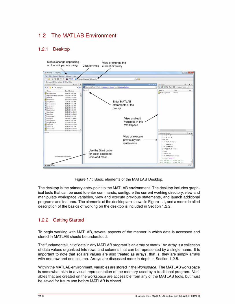
Figure 1.1: Basic elements of the MATLAB Desktop.

The desktop is the primary entry-point to the MATLAB environment. The desktop includes graph-ical tools that can be used to enter commands, configure the current working directory, view andmanipulate workspace variables, view and execute previous statements, and launch additionalprograms and features. The elements of the desktop are shown in Figure 1.1, and amore detaileddescription of the basics of working on the desktop is included in Section 1.2.2.

1.2.2 Getting Started

To begin working with MATLAB, several aspects of the manner in which data is accessed andstored in MATLAB should be understood.

The fundamental unit of data in anyMATLAB program is an array or matrix. An array is a collectionof data values organized into rows and columns that can be represented by a single name. It isimportant to note that scalars values are also treated as arrays, that is, they are simply arrayswith one row and one column. Arrays are discussed more in-depth in Section 1.2.5.

Within theMATLAB environment, variables are stored in theWorkspace. TheMATLABworkspaceis somewhat akin to a visual representation of the memory used by a traditional program. Vari-ables that are created on the workspace are accessible from any of the MATLAB tools, but mustbe saved for future use before MATLAB is closed.


The current working directory, which appears in the Current Directory tool on the desktop, iswhere data can be stored permanently for future use. The other location that is primarily accessedby MATLAB is the installation folder on the local machine where the functions that makeup themathematical function library are stored. These function can be opened and manipulated tocreate custom derivations of existing MATLAB commands.

1.2.3 Functions and Commands

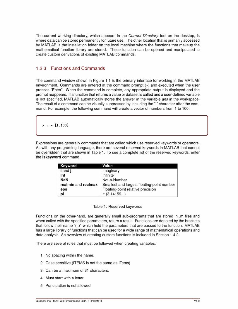
The command window shown in Figure 1.1 is the primary interface for working in the MATLABenvironment. Commands are entered at the command prompt (») and executed when the userpresses ”Enter”. When the command is complete, any appropriate output is displayed and theprompt reappears. If a function that returns a value or dataset is called and a user-defined variableis not specified, MATLAB automatically stores the answer in the variable ans in the workspace.The result of a command can be visually suppressed by including the ”;” character after the com-mand. For example, the following command will create a vector of numbers from 1 to 100:

v = [1:100];

Expressions are generally commands that are called which use reserved keywords or operators.As with any programing language, there are several reserved keywords in MATLAB that cannotbe overridden that are shown in Table 1. To see a complete list of the reserved keywords, enterthe iskeyword command.

Keyword Valuei and j ImaginaryInf InfiniteNaN Not-a-Numberrealmin and realmax Smallest and largest floating-point numbereps Floating-point relative precisionpi π (3.14159...)

Table 1: Reserved keywords

Functions on the other-hand, are generally small sub-programs that are stored in .m files andwhen called with the specified parameters, return a result. Functions are denoted by the bracketsthat follow their name ”(..)” which hold the parameters that are passed to the function. MATLABhas a large library of functions that can be used for a wide range of mathematical operations anddata analysis. An overview of creating custom functions is included in Section 1.4.2.

There are several rules that must be followed when creating variables:

1. No spacing within the name.

2. Case sensitive (ITEMS is not the same as ITems)

3. Can be a maximum of 31 characters.

4. Must start with a letter.

5. Punctuation is not allowed.


When changing the value of a variable, the new entry overwrites the original value. Keep in mindthat if a variable is changed, calculations must then be re-executed as MATLAB uses the value itknows at the time the command is evaluated.

1.2.4 Operators

The following are themost commonmathematical operators used to create MATLAB expressions:

Expression DefinitionA+B AdditionA-B SubtractionA*B MultiplicationA/B DivisionBˆ2 ExponentA’ Complex conjugate transpose

The majority of the commands listed above can be used for both scalar operations and matrixoperations. For example, 2 * 4 = 8 and at the same time A * B is the matrix multiplication of thematrices A and B. To perform array operations such as an element-wise array multiplication ordivision, include a ”.” before the operator. Perhaps the most important operator, however, is the%..% operator which denotes a single line comment.

1.2.5 Working with Arrays

The following commands are most commonly used to create, access and manipulate data arrays:

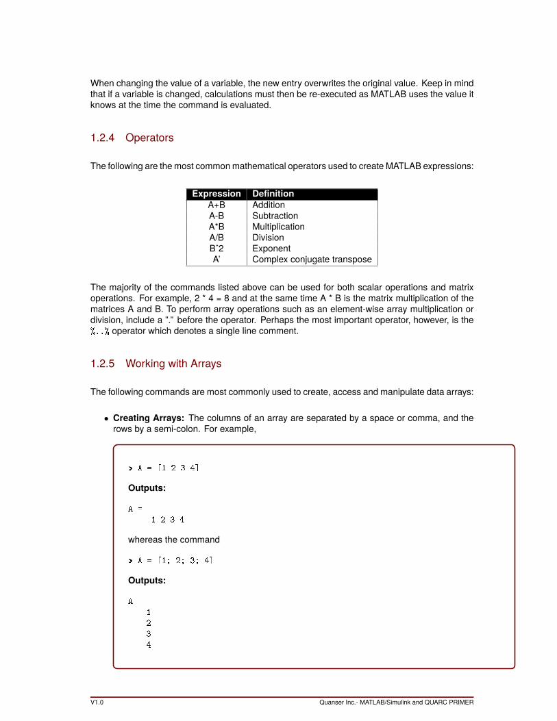
• Creating Arrays: The columns of an array are separated by a space or comma, and therows by a semi-colon. For example,

A = [1 2 3 4]

Outputs:

A =

1 2 3 4

whereas the command

A = [1; 2; 3; 4]

Outputs:

A =

1

2

3

4


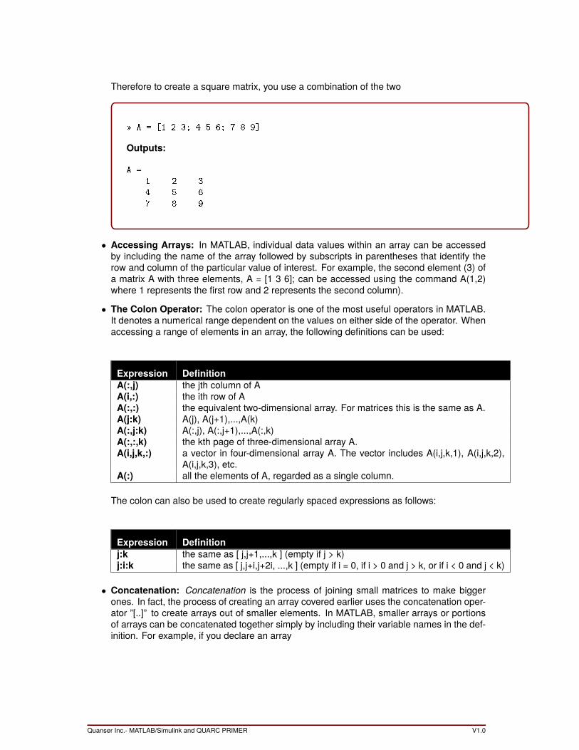
Therefore to create a square matrix, you use a combination of the two

A = [1 2 3; 4 5 6; 7 8 9]

Outputs:

A =

1 2 3

4 5 6

7 8 9

• Accessing Arrays: In MATLAB, individual data values within an array can be accessedby including the name of the array followed by subscripts in parentheses that identify therow and column of the particular value of interest. For example, the second element (3) ofa matrix A with three elements, A = [1 3 6]; can be accessed using the command A(1,2)where 1 represents the first row and 2 represents the second column).

• The Colon Operator: The colon operator is one of the most useful operators in MATLAB.It denotes a numerical range dependent on the values on either side of the operator. Whenaccessing a range of elements in an array, the following definitions can be used:

Expression DefinitionA(:,j) the jth column of AA(i,:) the ith row of AA(:,:) the equivalent two-dimensional array. For matrices this is the same as A.A(j:k) A(j), A(j+1),...,A(k)A(:,j:k) A(:,j), A(:,j+1),...,A(:,k)A(:,:,k) the kth page of three-dimensional array A.A(i,j,k,:) a vector in four-dimensional array A. The vector includes A(i,j,k,1), A(i,j,k,2),

A(i,j,k,3), etc.A(:) all the elements of A, regarded as a single column.

The colon can also be used to create regularly spaced expressions as follows:

Expression Definitionj:k the same as [ j,j+1,...,k ] (empty if j > k)j:i:k the same as [ j,j+i,j+2i, ...,k ] (empty if i = 0, if i > 0 and j > k, or if i < 0 and j < k)

• Concatenation: Concatenation is the process of joining small matrices to make biggerones. In fact, the process of creating an array covered earlier uses the concatenation oper-ator ”[..]” to create arrays out of smaller elements. In MATLAB, smaller arrays or portionsof arrays can be concatenated together simply by including their variable names in the def-inition. For example, if you declare an array


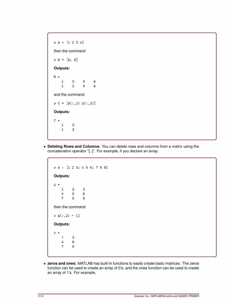
A = [1 2 3 4]

then the command

B = [A; A]

Outputs:

B =

1 2 3 4

1 2 3 4

and the command

C = [B(:,1) B(:,3)]

Outputs:

C =

1 3

1 3

• Deleting Rows and Columns: You can delete rows and columns from a matrix using theconcatenation operator ”[..]”. For example, if you declare an array:

A = [1 2 3; 4 5 6; 7 8 9]

Outputs:

A =

1 2 3

4 5 6

7 8 9

then the command

A(:,2) = []

Outputs:

A =

1 3

4 6

7 9

• zeros and ones: MATLAB has built-in functions to easily create basic matrices. The zerosfunction can be used to create an array of 0’s, and the ones function can be used to createan array of 1’s. For example,


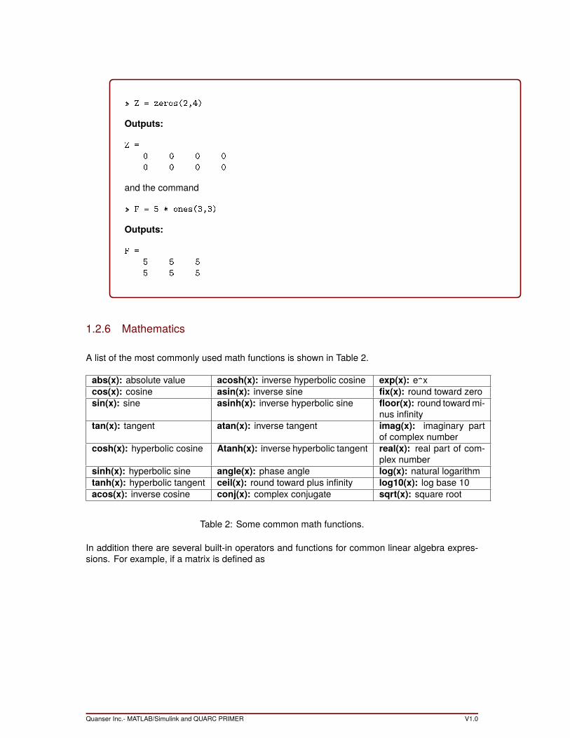
Z = zeros(2,4)

Outputs:

Z =

0 0 0 0

0 0 0 0

and the command

F = 5 * ones(3,3)

Outputs:

F =

5 5 5

5 5 5

1.2.6 Mathematics

A list of the most commonly used math functions is shown in Table 2.

abs(x): absolute value acosh(x): inverse hyperbolic cosine exp(x): e^xcos(x): cosine asin(x): inverse sine fix(x): round toward zerosin(x): sine asinh(x): inverse hyperbolic sine floor(x): round towardmi-

nus infinitytan(x): tangent atan(x): inverse tangent imag(x): imaginary part

of complex numbercosh(x): hyperbolic cosine Atanh(x): inverse hyperbolic tangent real(x): real part of com-

plex numbersinh(x): hyperbolic sine angle(x): phase angle log(x): natural logarithmtanh(x): hyperbolic tangent ceil(x): round toward plus infinity log10(x): log base 10acos(x): inverse cosine conj(x): complex conjugate sqrt(x): square root

Table 2: Some common math functions.

In addition there are several built-in operators and functions for common linear algebra expres-sions. For example, if a matrix is defined as


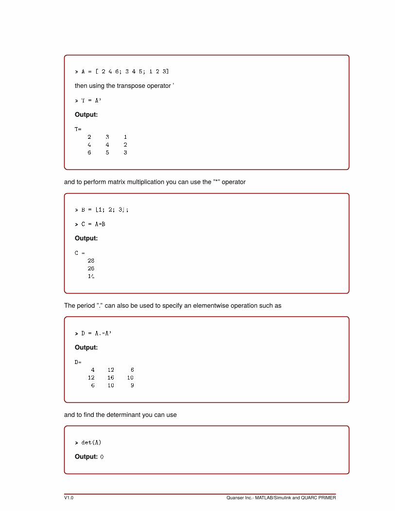
A = [ 2 4 6; 3 4 5; 1 2 3]

then using the transpose operator ’

T = A'

Output:

T=

2 3 1

4 4 2

6 5 3

and to perform matrix multiplication you can use the ”*” operator

B = [1; 2; 3];

C = A*B

Output:

C =

28

26

14

The period ”.” can also be used to specify an elementwise operation such as

D = A.*A'

Output:

D=

4 12 6

12 16 10

6 10 9

and to find the determinant you can use

det(A)

Output: 0


There are also several other functions for finding the inverse, row echelon form, eigenvalues, etc.

1.2.7 Polynomials

For the majority of operations that are performed on a polynomial expression, the polynomial isrepresented as a vector of the coefficients in descending order of power. For example, the poly-nomial x = s3 + 3s2 + 2s+ 1 would be entered as:

x = [1 3 2 1];

Zeros must be entered into the expression as place-holders if the polynomial is missing coeffi-cients. For example, x = x4 + 1 would be entered as

x = [1 0 0 0 1];

There are several functions that can be used to perform common tasks with polynomials. Forexample, to find the value of the polynomial p(x) = 3x2 + 2x+ 1 at x = 3, 4, and 5 you would usethe function polyval as

p = [3 2 1];

polyval(p,[3 4 5])

Output:

ans =

86 162 262

To find the roots of a polynomial, use the function roots as

p = [4 8 2];

roots(p)

Output:

ans =

-1.7071

-0.2929


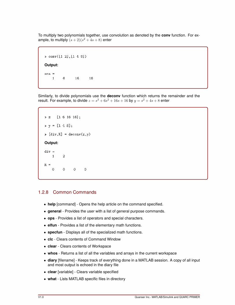
To multiply two polynomials together, use convolution as denoted by the conv function. For ex-ample, to multiply (s+ 2)(s2 + 4s+ 8) enter

conv([1 2],[1 4 8])

Output:

ans =

1 6 16 16

Similarly, to divide polynomials use the deconv function which returns the remainder and theresult. For example, to divide z = s3 + 6s2 + 16s+ 16 by y = s2 + 4s+ 8 enter

z = [1 6 16 16];

y = [1 4 8];

[div,R] = deconv(z,y)

Output:

div =

1 2

R =

0 0 0 0

1.2.8 Common Commands

• help [command] - Opens the help article on the command specified.

• general - Provides the user with a list of general purpose commands.

• ops - Provides a list of operators and special characters.

• elfun - Provides a list of the elementary math functions.

• specfun - Displays all of the specialized math functions.

• clc - Clears contents of Command Window

• clear - Clears contents of Workspace

• whos - Returns a list of all the variables and arrays in the current workspace

• diary [filename] - Keeps track of everything done in a MATLAB session. A copy of all inputand most output is echoed in the diary file

• clear [variable] - Clears variable specified

• what - Lists MATLAB specific files in directory


1.3 Figures and Graphing

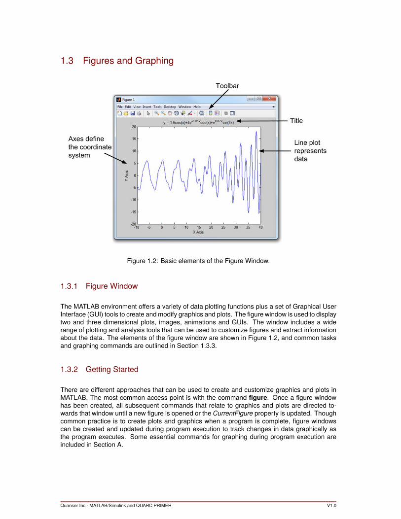
Figure 1.2: Basic elements of the Figure Window.

1.3.1 Figure Window

The MATLAB environment offers a variety of data plotting functions plus a set of Graphical UserInterface (GUI) tools to create andmodify graphics and plots. The figure window is used to displaytwo and three dimensional plots, images, animations and GUIs. The window includes a widerange of plotting and analysis tools that can be used to customize figures and extract informationabout the data. The elements of the figure window are shown in Figure 1.2, and common tasksand graphing commands are outlined in Section 1.3.3.


There are different approaches that can be used to create and customize graphics and plots inMATLAB. The most common access-point is with the command figure. Once a figure windowhas been created, all subsequent commands that relate to graphics and plots are directed to-wards that window until a new figure is opened or the CurrentFigure property is updated. Thoughcommon practice is to create plots and graphics when a program is complete, figure windowscan be created and updated during program execution to track changes in data graphically asthe program executes. Some essential commands for graphing during program execution areincluded in Section A.


1.3.3 Creating 2-D Plots

The most commonly used functions for creating plots are listed below. In addition to these func-tions, several of the MATLAB toolboxes include specialized functions for creating topical plots forspecific datasets. For example, the bode function which is detailed in 1.5 can be used to quicklycreate bode plots for system analysis.

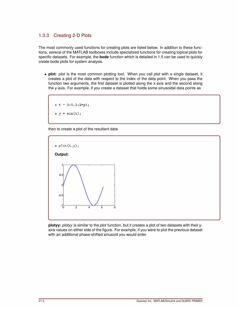
• plot: plot is the most common plotting tool. When you call plot with a single dataset, itcreates a plot of the data with respect to the index of the data point. When you pass thefunction two arguments, the first dataset is plotted along the x-axis and the second alongthe y-axis. For example, if you create a dataset that holds some sinusoidal data points as

t = 0:0.1:2*pi;

y = sin(t);

then to create a plot of the resultant data

plot(t,y);

Output:

plotyy: plotyy is similar to the plot function, but it creates a plot of two datasets with their y-axis values on either side of the figure. For example, if you were to plot the previous datasetwith an additional phase-shifted sinusoid you would enter


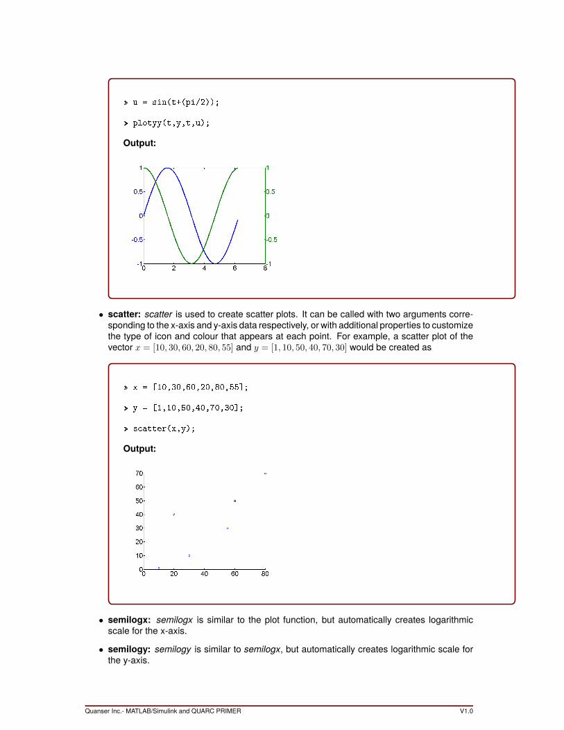
u = sin(t+(pi/2));

plotyy(t,y,t,u);

Output:

• scatter: scatter is used to create scatter plots. It can be called with two arguments corre-sponding to the x-axis and y-axis data respectively, or with additional properties to customizethe type of icon and colour that appears at each point. For example, a scatter plot of thevector x = [10, 30, 60, 20, 80, 55] and y = [1, 10, 50, 40, 70, 30] would be created as

x = [10,30,60,20,80,55];

y = [1,10,50,40,70,30];

scatter(x,y);

Output:

• semilogx: semilogx is similar to the plot function, but automatically creates logarithmicscale for the x-axis.

• semilogy: semilogy is similar to semilogx, but automatically creates logarithmic scale forthe y-axis.


1.3.4 Managing Figures

Some essential commands for creating and customizing figures and plots are listed below. Someof these functions and commands can also be accessed through the figure window.

• hold: The hold command is used to tell MATLAB to graph subsequent plots in the currentfigure window. The property is turned on by calling hold on, and turned off by calling hold off.If the property is turned on, additional plots are automatically coloured differently to avoidconfusion. To retain the current line and colour settings, the hold all command is used. Forexample, to graph the two sinusoids y = sin(t) +π /2 and j = sin(t) you could enter

t = 0:0.1:2*pi();

y = sin(t)+2;

j = sin(t);

plot(t,y);

hold on

plot(t,j);

Output:

• axis: The axis command is used to set the scaling and appearance of the axes on thecurrent plot. The most common syntax is axis([xmin xmax ymin ymax]) where the min andmax values correspond to the desired axes boundaries.

• xlabel/ylabel/zlabel: The label commands are used to set the title of the specified axis.For example, the command xlabel(’Time (s)’); will create or modify the title of the x-axis to”Time (s)”.

• title: The title command is used to create or modify the title of the plot.

• clf: Calling the clf command clears the current figure.

• close all: Calling the close all command closes all figure windows.


1.4 Programming

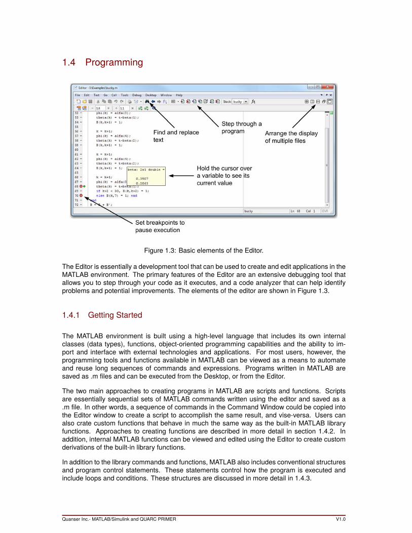
Figure 1.3: Basic elements of the Editor.

The Editor is essentially a development tool that can be used to create and edit applications in theMATLAB environment. The primary features of the Editor are an extensive debugging tool thatallows you to step through your code as it executes, and a code analyzer that can help identifyproblems and potential improvements. The elements of the editor are shown in Figure 1.3.


The MATLAB environment is built using a high-level language that includes its own internalclasses (data types), functions, object-oriented programming capabilities and the ability to im-port and interface with external technologies and applications. For most users, however, theprogramming tools and functions available in MATLAB can be viewed as a means to automateand reuse long sequences of commands and expressions. Programs written in MATLAB aresaved as .m files and can be executed from the Desktop, or from the Editor.

The two main approaches to creating programs in MATLAB are scripts and functions. Scriptsare essentially sequential sets of MATLAB commands written using the editor and saved as a.m file. In other words, a sequence of commands in the Command Window could be copied intothe Editor window to create a script to accomplish the same result, and vise-versa. Users canalso crate custom functions that behave in much the same way as the built-in MATLAB libraryfunctions. Approaches to creating functions are described in more detail in section 1.4.2. Inaddition, internal MATLAB functions can be viewed and edited using the Editor to create customderivations of the built-in library functions.

In addition to the library commands and functions, MATLAB also includes conventional structuresand program control statements. These statements control how the program is executed andinclude loops and conditions. These structures are discussed in more detail in 1.4.3.


1.4.2 User-Defined Functions

The fundamental difference between functions and scripts is that functions accept and returnparameters when they are called, whereas scripts simply execute their command sequence. Tocreate and run a script you simply write the program in the editor, and save the .m file in thecurrent directory. You can then type in the name of the script at the command prompt, or click onthe Run button on the editor menubar.

Functions on the other hand are denoted by the command function and are declared as follows:function [return_parameters] = function_name(input_parameters)

%Code goes here...

end

Variables that are passed into a function as arguments are accessed using the declarations inthe prototype (function command). Parameters that are returned from a function hold the value ofthe return variable when the function execution is complete. For example, the following functionreturns the root-mean-square (quadratic mean) of a set of numbers:

function [rms] = calculate(values)

rms = sqrt(sum(values.2)/length(values));

end

The following rules apply to user-defined functions:

• The first few lines of the function program should be comments for clarification purposes.

• The only information returned from the function is contained in the output argument(s).

• Variable names can be used in both a function and the program that references it.

• When a function that returns more than one variable is called, all return parameters mustbe specified or it will only return only the fist parameter. For example, the function

function [dist,vel,accel] = motion(x)

...

end

returns three parameters, but when called using the command

result = motion(x);

it will only return the first value. For all three return parameters it must be called as


[var1, var2, var3] = motion(x);

1.4.3 Program Control

The two most important elements of program control are conditional statements and loops. Thetwo types of conditional statements are if statements and switch statements. The two types ofloops are for statements and while statements. The elements of each are listed below:

• if, else, and elseif: The if statement (which may include else or elseif ) enables you toselect at run-time which block of code is executed. The selection of the particular codeblock is made depending on the condition specified in the statement using the relationaloperators listed in Table 3 and the logical operators listed in Table 4. Execution of thecondition statementif (logical_expression)

statements

end

can therefore be described verbally as:if condition_1 is (greater than/less than/equal to) ... condition_2 (and/or)

... then

% Execute this code block

(else/elseif condition_3)% Execute this code block

end

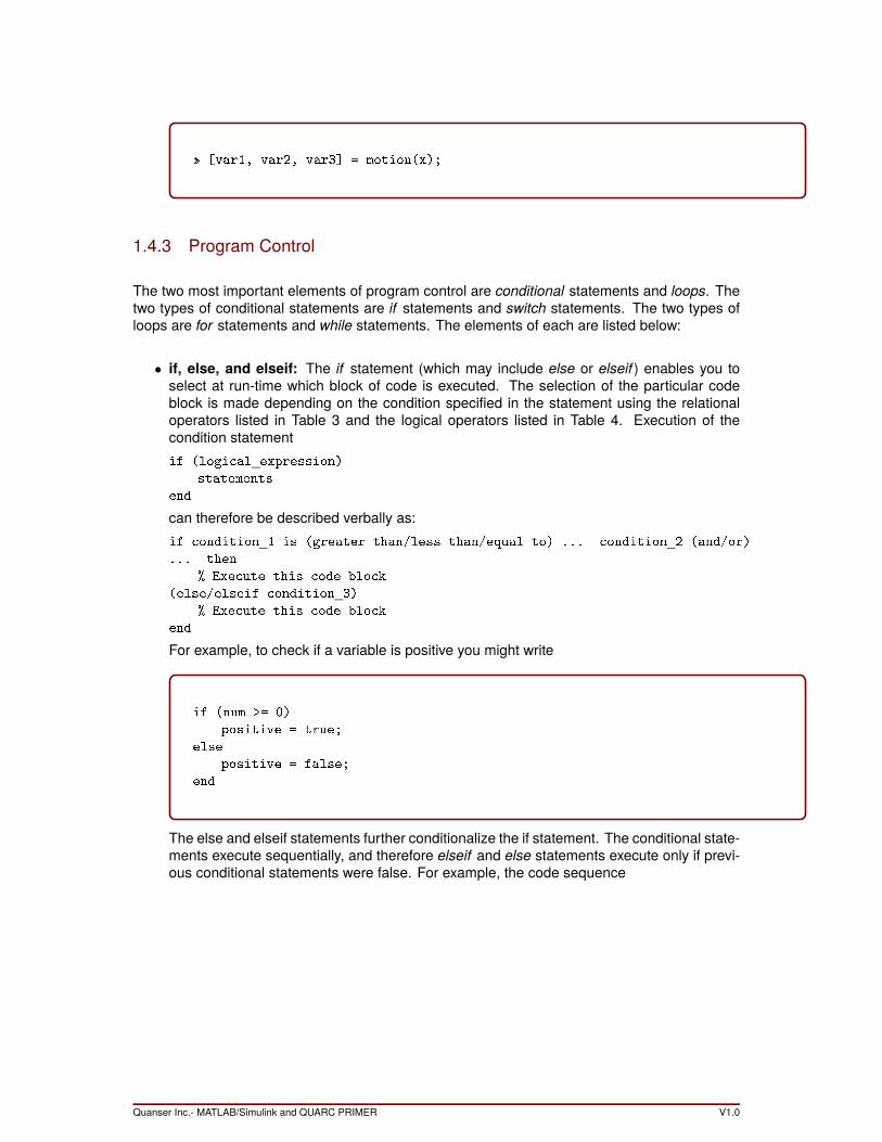
For example, to check if a variable is positive you might write

if (num >= 0)

positive = true;

else

positive = false;

end

The else and elseif statements further conditionalize the if statement. The conditional state-ments execute sequentially, and therefore elseif and else statements execute only if previ-ous conditional statements were false. For example, the code sequence


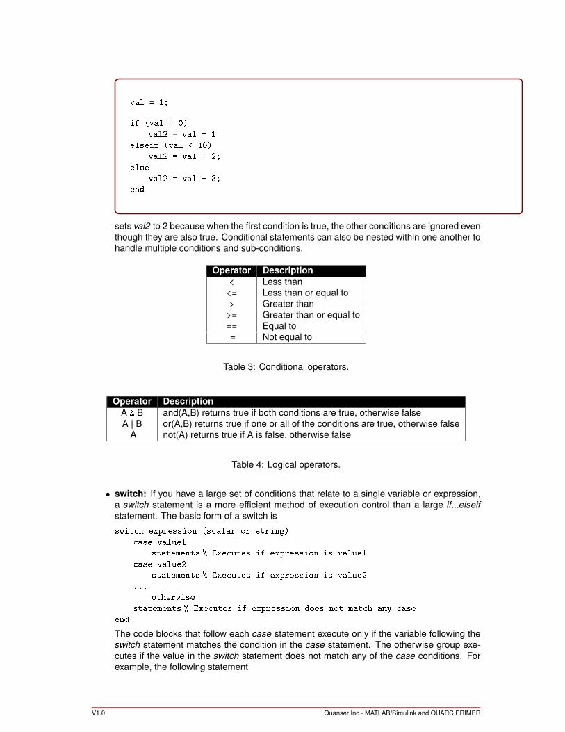
val = 1;

if (val > 0)

val2 = val + 1

elseif (val < 10)

val2 = val + 2;

else

val2 = val + 3;

end

sets val2 to 2 because when the first condition is true, the other conditions are ignored eventhough they are also true. Conditional statements can also be nested within one another tohandle multiple conditions and sub-conditions.

Operator Description< Less than<= Less than or equal to> Greater than>= Greater than or equal to== Equal to= Not equal to

Table 3: Conditional operators.

Operator DescriptionA & B and(A,B) returns true if both conditions are true, otherwise falseA | B or(A,B) returns true if one or all of the conditions are true, otherwise falseA not(A) returns true if A is false, otherwise false

Table 4: Logical operators.

• switch: If you have a large set of conditions that relate to a single variable or expression,a switch statement is a more efficient method of execution control than a large if...elseifstatement. The basic form of a switch isswitch expression (scalar_or_string)

case value1

statements % Executes if expression is value1

case value2

statements % Executes if expression is value2

...

otherwise

statements % Executes if expression does not match any case

end

The code blocks that follow each case statement execute only if the variable following theswitch statement matches the condition in the case statement. The otherwise group exe-cutes if the value in the switch statement does not match any of the case conditions. Forexample, the following statement


switch num

case -1

val = 'negative one';

case 0

val = 'zero';

case 1

val = 'positive one';

otherwise

val = 'other value';

end

will compare the value of num to the values -1, 0, and 1 and set val to the appropriate string.

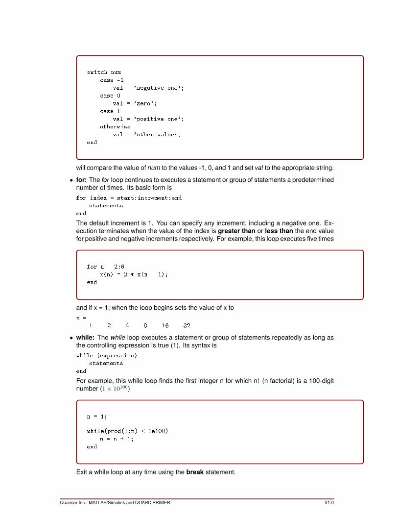
• for: The for loop continues to executes a statement or group of statements a predeterminednumber of times. Its basic form isfor index = start:increment:end

statements

end

The default increment is 1. You can specify any increment, including a negative one. Ex-ecution terminates when the value of the index is greater than or less than the end valuefor positive and negative increments respectively. For example, this loop executes five times

for n = 2:6

x(n) = 2 * x(n - 1);

end

and if x = 1; when the loop begins sets the value of x tox =

1 2 4 8 16 32

• while: The while loop executes a statement or group of statements repeatedly as long asthe controlling expression is true (1). Its syntax iswhile (expression)

statements

end

For example, this while loop finds the first integer n for which n! (n factorial) is a 100-digitnumber (1× 10100)

n = 1;

while(prod(1:n) < 1e100)

n = n + 1;

end

Exit a while loop at any time using the break statement.


1.5 Control Systems Toolbox

The Control System Toolbox is a set of functions written in the MATLAB language that make itconvenient to build the system models and perform the analyses that are used in control systemsengineering. A list of the most common commands for systems analysis, modeling and controlare listed in section Section 1.5.1.

1.5.1 Common Commands

• sys=tf(num,den): Given numerator and denominator polynomials, tf creates the systemmodel as a transfer function object. The continuous-time transfer function is created withnumerators (num) and denominators (den). The transfer function (TF) object can then beused in conjunction with several additional analysis tools.

• T=feedback(G,H): Given the models of two systems as TF objects, (G,H), feedback re-turns the model of the closed-loop system. Negative feedback is assumed, but an optionalargument can be used to handle the positive feedback case.

• y=step(T): Given a continuous system, step returns the response to a unit step input. Ifstep is called without output arguments, the function creates a plot of the response.

• y=impulse(T): Given a continuous system, impulse returns the response to a unit stepinput. If step is called without output arguments, the function creates a plot of the response.

• output=lsim(sys,u,t): Given a continuous LTI system, a vector of input values (u), a vectorof time points (t) and a set of initial conditions, lsim returns the time response. lsim plots thetime response of the LTI model sys to the input signal described by [u,t]. The time vector(t), consists of regularly spaced time samples and the input (u) is a matrix with as manycolumns as inputs whose ith row specifies the input value at time t.

• damp(T): Given an LTI system, damp returns the closed loop system poles, their dampingratios and their natural frequencies. The output is three columns in the order of poles,damping ratios and natural frequencies respectively.

• rlocus(F): Given a transfer function (F(s)) of an open-loop system, rlocus produces a rootlocus plot that shows the locations of the closed-loop poles in the s-plane as the loop gainvaries from 0 to∞.

• [gainsk,polesk]=rlocfind(F(s)): Given a transfer function (F(s)) from the characteristicequation, rlocfind allows the user to select any point on the locus with the mouse and re-turns the value of the loop gain that will make that point be a closed-loop pole (gainsk). Italso returns the values of all the closed-loop poles for that gain value (polesk).

• bode(G,w): This commands generates a Bode plot of the system (G) over the frequencyrange (w) in rad/s. The magnitude |G(jω)| is plotted in decibels (dB), and the phase indegrees. If called with the return arguments [mag,phase], this command returns the mag-nitude in the column vector [mag], and the phase angles in degrees in the column vector[phase].

• w = logspace(a,b,n): Generates frequency values that are uniformly spaced on the log-arithmic scale. It returns a row vector containing n points from a to b that are uniformlyspaced on the logarithmic scale.

• margin(G): Generates a bode plot with the margins and crossover frequencies indicated.

• [gm,pm, p, g] = margin(G): Generates the output variables, gain margin (gm), phase mar-gin (pm), phase crossover frequency (p), and gain crossover frequency (g).


1.6 Example 1 - Toy Train

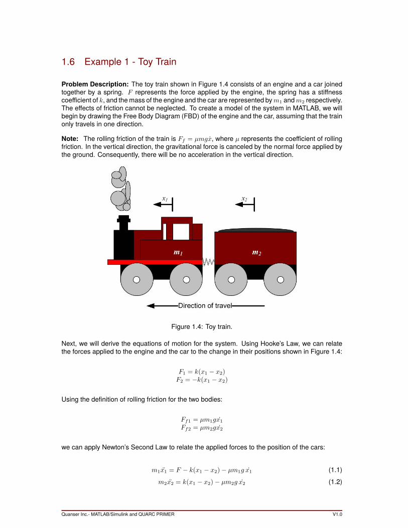
Problem Description: The toy train shown in Figure 1.4 consists of an engine and a car joinedtogether by a spring. F represents the force applied by the engine, the spring has a stiffnesscoefficient of k, and themass of the engine and the car are represented bym1 andm2 respectively.The effects of friction cannot be neglected. To create a model of the system in MATLAB, we willbegin by drawing the Free Body Diagram (FBD) of the engine and the car, assuming that the trainonly travels in one direction.

Note: The rolling friction of the train is Ff = µmgx, where µ represents the coefficient of rollingfriction. In the vertical direction, the gravitational force is canceled by the normal force applied bythe ground. Consequently, there will be no acceleration in the vertical direction.

Figure 1.4: Toy train.

Next, we will derive the equations of motion for the system. Using Hooke’s Law, we can relatethe forces applied to the engine and the car to the change in their positions shown in Figure 1.4:

F1 = k(x1 − x2)F2 = −k(x1 − x2)

Using the definition of rolling friction for the two bodies:

Ff1 = µm1gx1Ff2 = µm2gx2

we can apply Newton’s Second Law to relate the applied forces to the position of the cars:

m1x1 = F − k(x1 − x2)− µm1g x1 (1.1)

m2x2 = k(x1 − x2)− µm2g x2 (1.2)


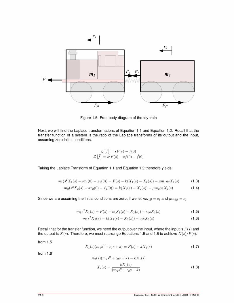
Figure 1.5: Free body diagram of the toy train

Next, we will find the Laplace transformations of Equation 1.1 and Equation 1.2. Recall that thetransfer function of a system is the ratio of the Laplace transforms of its output and the input,assuming zero initial conditions.

L[f]

= sF (s)− f(0)

L[f]

= s2F (s)− sf(0)− f(0)

Taking the Laplace Transform of Equation 1.1 and Equation 1.2 therefore yields:

m1(s2X1(s)− sx1(0)− x1(0)) = F (s)− k(X1(s)−X2(s))− µm1gsX1(s) (1.3)

m2(s2X2(s)− sx2(0)− x2(0)) = k(X1(s)−X2(s))− µm2gsX2(s) (1.4)

Since we are assuming the initial conditions are zero, if we let µm1g = c1 and µm2g = c2

m1s2X1(s) = F (s)− k(X1(s)−X2(s))− c1sX1(s) (1.5)

m2s2X2(s) = k(X1(s)−X2(s))− c2sX2(s) (1.6)

Recall that for the transfer function, we need the output over the input, where the input is F (s) andthe output is X(s). Therefore, we must rearrange Equations 1.5 and 1.6 to achieve X(s)/F (s).

from 1.5X1(s)(m1s

2 + c1s+ k) = F (s) + kX2(s) (1.7)

from 1.6X2(s)(m2s

2 + c2s+ k) = kX1(s)

X2(s) =kX1(s)

(m2s2 + c2s+ k)(1.8)


sub Equation 1.8 into Equation 1.7 and rearranging yields

X1(s)(m1s2 + c1s+ k) = F (s) + k

(kX1(s)

m2s2 + c2s+ k

)X1(s)

(m1s2 + c1s+ k − k2

m2s2 + c2s+ k

)= F (s)

X1(s)

F (s)=

1

m1s2 + c1s+ k − k2

(m2s2+c2s+k)

orX1(s)

F (s)=

m2s2 + c2s+ k

m1m2s4 + (m1c2 +m2c1)s3 + (m1k + c1c2 +m2k)s2 + (c1k + c2k)s(1.9)

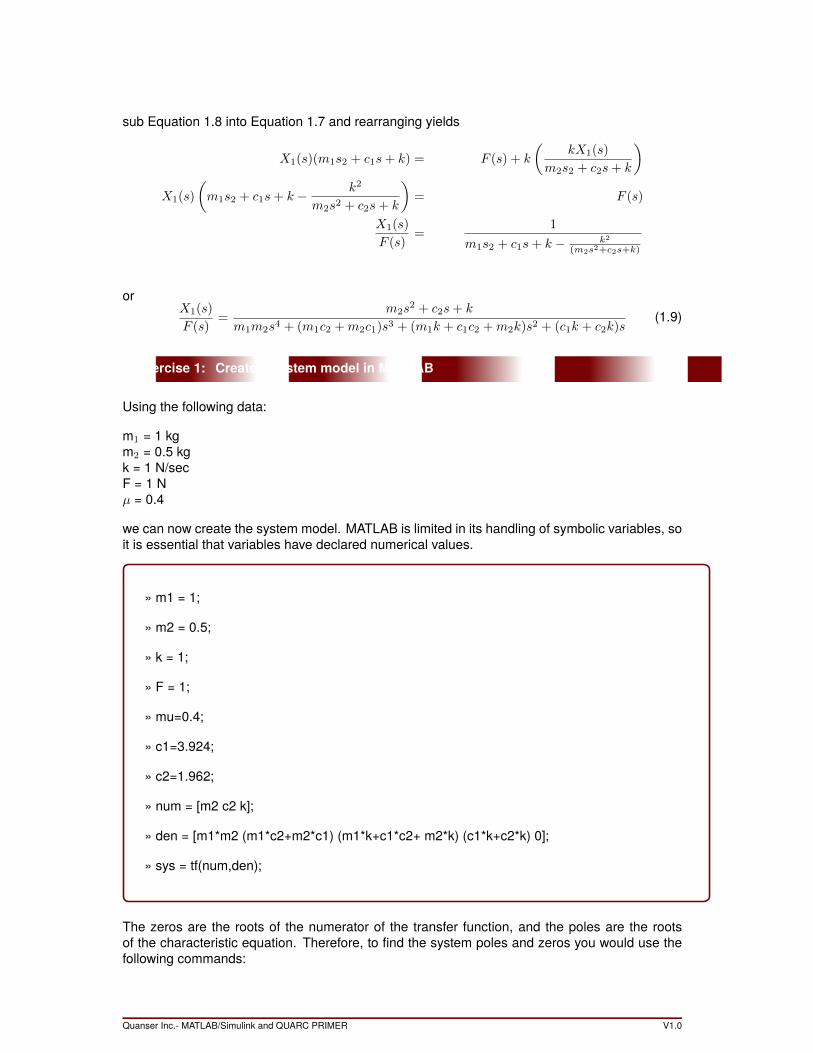
Exercise 1: Create a system model in MATLAB

Using the following data:

m1 = 1 kgm2 = 0.5 kgk = 1 N/secF = 1 Nµ = 0.4

we can now create the system model. MATLAB is limited in its handling of symbolic variables, soit is essential that variables have declared numerical values.

» m1 = 1;

» m2 = 0.5;

» k = 1;

» F = 1;

» mu=0.4;

» c1=3.924;

» c2=1.962;

» num = [m2 c2 k];

» den = [m1*m2 (m1*c2+m2*c1) (m1*k+c1*c2+ m2*k) (c1*k+c2*k) 0];

» sys = tf(num,den);

The zeros are the roots of the numerator of the transfer function, and the poles are the rootsof the characteristic equation. Therefore, to find the system poles and zeros you would use thefollowing commands:


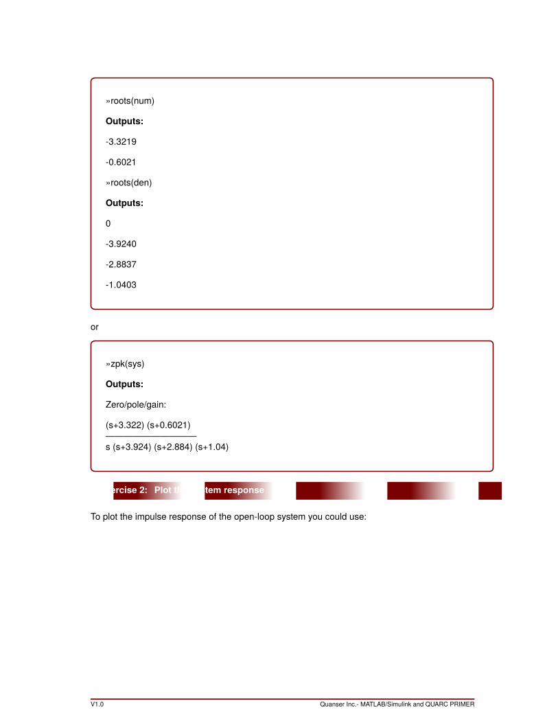
»roots(num)

Outputs:

-3.3219

-0.6021

»roots(den)

Outputs:

0

-3.9240

-2.8837

-1.0403

or

»zpk(sys)

Outputs:

Zero/pole/gain:

(s+3.322) (s+0.6021)——————————s (s+3.924) (s+2.884) (s+1.04)

Exercise 2: Plot the system response

To plot the impulse response of the open-loop system you could use:


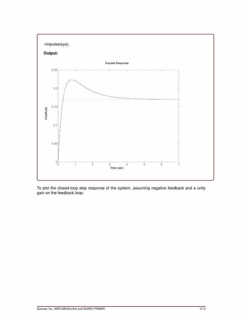
»impulse(sys);

Output:

To plot the closed-loop step response of the system, assuming negative feedback and a unitygain on the feedback loop:


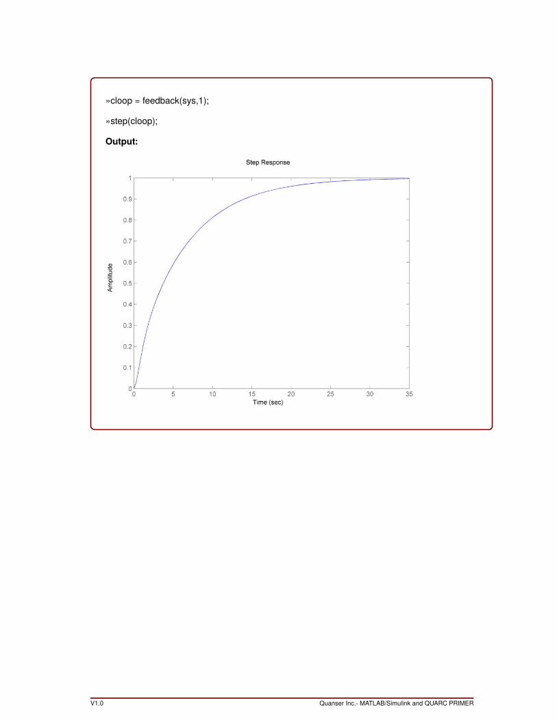
»cloop = feedback(sys,1);

»step(cloop);

Output:


2 Simulink

2.1 Introduction

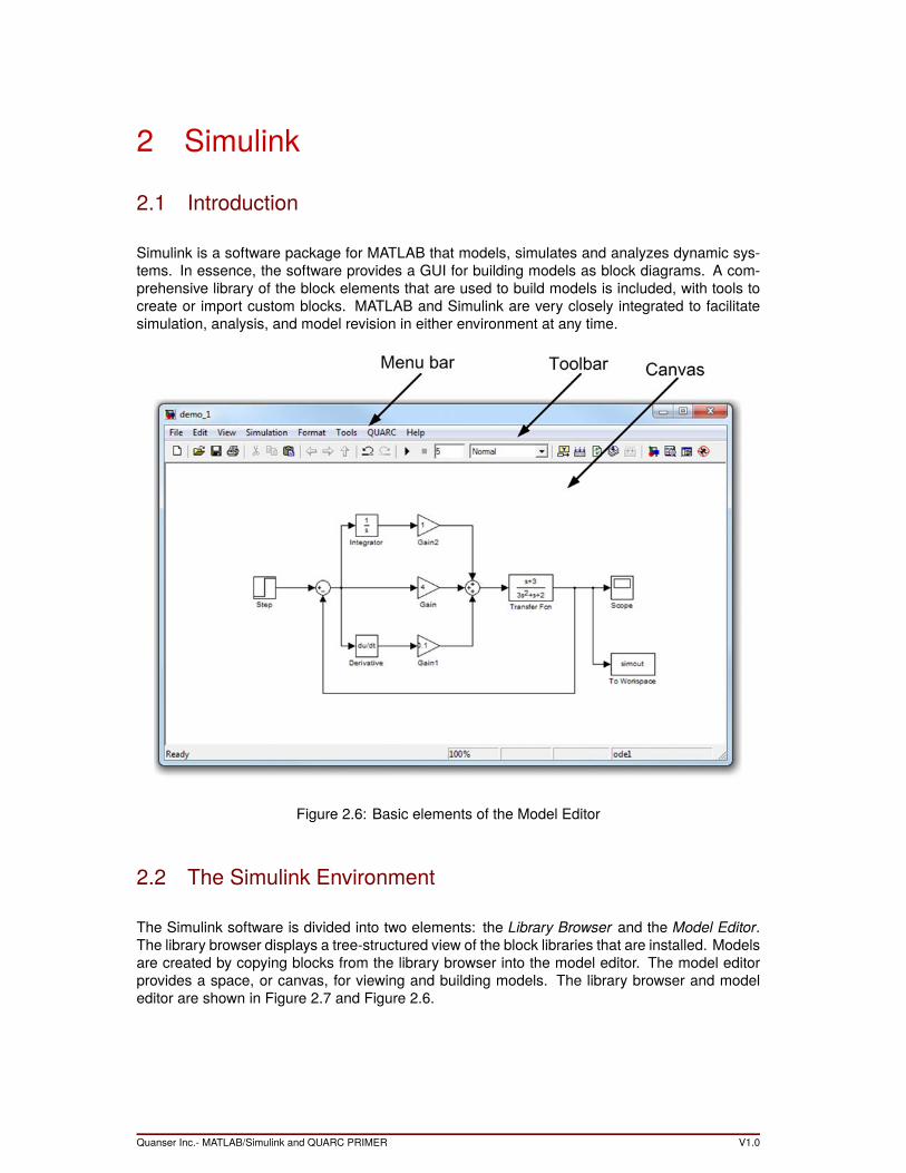
Simulink is a software package for MATLAB that models, simulates and analyzes dynamic sys-tems. In essence, the software provides a GUI for building models as block diagrams. A com-prehensive library of the block elements that are used to build models is included, with tools tocreate or import custom blocks. MATLAB and Simulink are very closely integrated to facilitatesimulation, analysis, and model revision in either environment at any time.

Figure 2.6: Basic elements of the Model Editor

2.2 The Simulink Environment

The Simulink software is divided into two elements: the Library Browser and the Model Editor.The library browser displays a tree-structured view of the block libraries that are installed. Modelsare created by copying blocks from the library browser into the model editor. The model editorprovides a space, or canvas, for viewing and building models. The library browser and modeleditor are shown in Figure 2.7 and Figure 2.6.


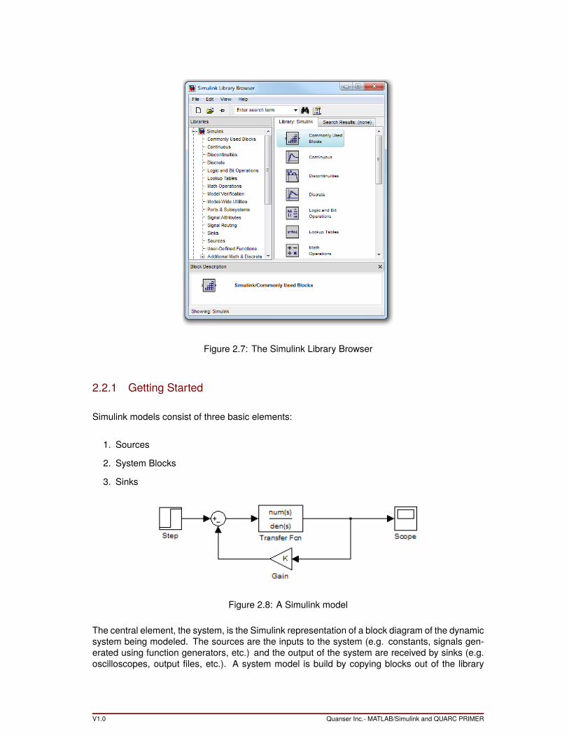
Figure 2.7: The Simulink Library Browser


Simulink models consist of three basic elements:

1. Sources

2. System Blocks

3. Sinks

Figure 2.8: A Simulink model

The central element, the system, is the Simulink representation of a block diagram of the dynamicsystem being modeled. The sources are the inputs to the system (e.g. constants, signals gen-erated using function generators, etc.) and the output of the system are received by sinks (e.g.oscilloscopes, output files, etc.). A system model is build by copying blocks out of the library


browser and into the model editor. They are then connected together by drawing connectors be-tween the blocks. More details on creating system models are listed in Section 2.3, and a samplemodel is shown in Figure 2.8.

Once the model is complete, a basic simulation can be run by clicking on the Start Simulationbutton on the toolbar. The simulation will run for the amount of time listed next to the simula-tion controls, using the simulation model listed in the adjacent combo-box. The progress of thesimulation appears in a progress bar at the bottom of the window. A more detailed account ofconfiguring and running a simulation is presented in Section 2.4.

2.3 Building a Model

2.3.1 Sources

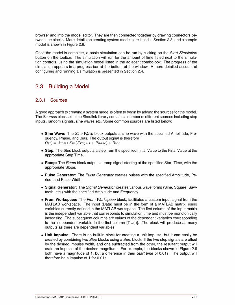
A good approach to creating a systemmodel is often to begin by adding the sources for the model.The Sources blockset in the Simulink library contains a number of different sources including stepinputs, random signals, sine waves etc. Some common sources are listed below:

• Sine Wave: The Sine Wave block outputs a sine wave with the specified Amplitude, Fre-quency, Phase, and Bias. The output signal is thereforeO(t) = Amp ∗ Sin(Freq ∗ t+ Phase) +Bias

• Step: The Step block outputs a step from the specified Initial Value to the Final Value at theappropriate Step Time.

• Ramp: The Ramp block outputs a ramp signal starting at the specified Start Time, with theappropriate Slope.

• Pulse Generator: The Pulse Generator creates pulses with the specified Amplitude, Pe-riod, and Pulse Width.

• Signal Generator: The Signal Generator creates various wave forms (Sine, Square, Saw-tooth, etc.) with the specified Amplitude and Frequency.

• From Workspace: The From Workspace block, facilitates a custom input signal from theMATLAB workspace. The input (Data) must be in the form of a MATLAB matrix, usingvariables currently defined in the MATLAB workspace. The first column of the input matrixis the independent variable that corresponds to simulation time and must be monotonicallyincreasing. The subsequent columns are values of the dependent variables correspondingto the independent variable in the first column [T,U(t)]. The block will produce as manyoutputs as there are dependent variables.

• Unit Impulse: There is no built-in block for creating a unit impulse, but it can easily becreated by combining two Step blocks using a Sum block. If the two step signals are offsetby the desired impulse width, and one subtracted from the other, the resultant output willcrate an impulse of the desired magnitude. For example, the blocks shown in Figure 2.9both have a magnitude of 1, but a difference in their Start time of 0.01s. The output willtherefore be a impulse of 1 for 0.01s.


Figure 2.9: Impulse Signal

2.3.2 Building a System Model

Once the sources for the model are in place, it is time to assemble the blocks that make-up thedynamic model of the system. The most common libraries and block sets that are used to buildsystem models are listed below.

• Commonly UsedBlocks: TheCommonly Used Blocks library includes themost commonlyused elements of other libraries. It is always a good place to start when searching for aparticular block or function. Most blocks in the library are straight-forward (Gain, Constant,Integrator, etc.) but others are a little more complicated and are outlined below:

– Mux/Demux: TheMux and Demux multiplex scalar or vector signals. For example, tosplit a feedback signal to feed into separate elements of a controller, a Demux couldbe used. To combine the separate signals together into a 2-dimensional vector to passto a Scope, a Mux could be utilized.

– Subsystem: The Subsystem block contains a separate model (or models) as a sub-element of the overall model. The contents of the subsystem are treated in the samemanner as the overall model, with data passed in and out of the system using inputand output blocks.

– In1/Out1: The In1 and Out1 blocks are used as an input port for subsystems or mod-els.

– Data Type Convert: TheData Type Convert block is a quantization block that converts”real-world” values input into the block to the proper data-type and scaling of the output.Normally, the properties of the output data type are automatically configured throughinheritance.


• Continuous: The Continuous library provides a set of blocks to create continuous timesystem models. These blocks include basic elements such as a derivative, integrator, anddelays. The library also includes complete system model blocks including a state-space,transfer function and zero-pole block. The system model blocks can be treated in the sameway as the MATLAB equivalents, with the appropriate parameters input as polynomial vec-tors.

• Discontinuities: The Discontinuities library includes several blocks for describing discon-tinuous or non-linear system elements including friction, backlash, saturation and dead-zones.

• Discrete: The Discrete library provides many of the same elements as the Continuouslibrary, but in discrete (sampled) time. The library also includes several filters and zero/first-order holds.

• Math Operations: TheMath Operations library includes operators for performing commonmathematical functions including addition, subtraction, products, trigonometry, polynomi-als, and exponents. The library also includes equivalent operations for signals includingsummation and gain blocks.

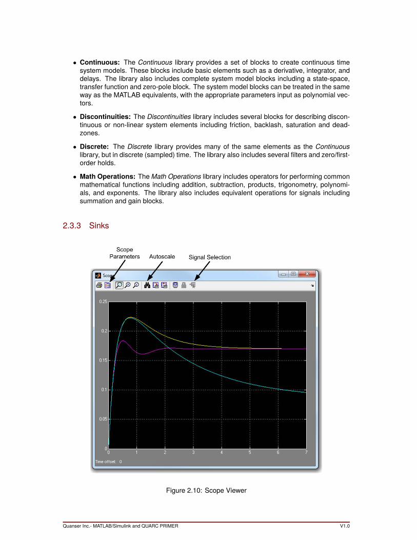
2.3.3 Sinks

Figure 2.10: Scope Viewer


Sinks provide the means to store and/or view model data. The most common approaches toviewing and storing data are to either send the data to the MATLAB workspace using the ToWorkspace block, or using a Scope.

The scope block emulates an oscilloscope thereby producing plots of the input data. The ScopeParameters dialog allows users to customize the axis properties, sampling, and data history set-tings.

• The horizontal and vertical axis ranges of the scope can be set to any desired values.

• The vertical axis displays the actual value of the signal, and the horizontal axis representstime. If the time range is set to ’auto’, the range will be the same as the simulation duration.

• The axes can also be auto adjusted to match the magnitude of the signal by clicking on theAuto Scale button on the toolbar (Binoculars).

2.4 Simulating a System Model

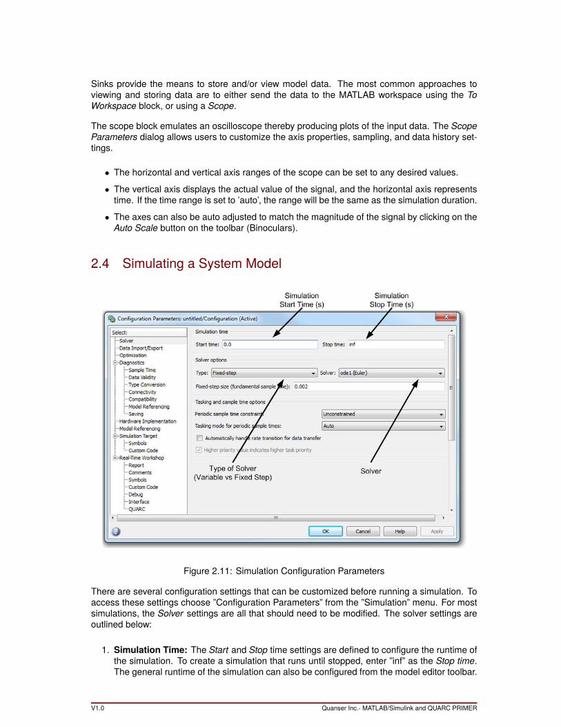
Figure 2.11: Simulation Configuration Parameters

There are several configuration settings that can be customized before running a simulation. Toaccess these settings choose ”Configuration Parameters” from the ”Simulation” menu. For mostsimulations, the Solver settings are all that should need to be modified. The solver settings areoutlined below:

1. Simulation Time: The Start and Stop time settings are defined to configure the runtime ofthe simulation. To create a simulation that runs until stopped, enter ”inf” as the Stop time.The general runtime of the simulation can also be configured from the model editor toolbar.


2. Solver Options: The Solver Options section provides configuration settings for the integra-tion and solver used in the simulation.Fixed-step solvers use the specified step size for solving the model. The step size can beviewed as the fundamental sample time of the system. A variable-step solver continuallyadjusts the integration step size within the provided bounds to maximize efficiency whilemaintaining the specified accuracy. Generally, the performance of a simulation is inverselyproportional to the step-size and the complexity of the solver.

(a) To choose a fixed-step solver, the most efficient method is to start by modeling thesystem using a variable-step solver to achieve the level of accuracy that you desire.

(b) Next, use ode1 to simulate the model, and compare the results with the variable-stepsimulation.

(c) If the results are within your desired level of accuracy, then ode1 is the correct solversince it is the simplest and therefore most efficient solver.

(d) If the results of the ode1 simulation are not accurate enough, then experiment with themore complex solvers until the most efficient solver is found that meets the accuracyrequirements.

(e) Choosing a variable-step solver can be performed in much the same manner, thoughif the model does not define any states, a discrete solver will be used.

Once the simulation configuration settings are determined, the simulation can be started by click-ing on the Start simulation button on the toolbar (triangle), or by choosing ”Start” from the ”Sim-ulation” menu. To stop the simulation click on the Stop button on the toolbar (square), or choose”Stop” from the menu. The simulation can also be paused by clicking on the start button duringa simulation.

2.5 Tips and Tricks

• The default orientation of all the blocks is with the input ports on the left edge of the blockand the output ports on the right edge. To flip blocks, click on the block selected, then goto Format | Flip Block or press Ctrl+I.

• To splice a signal line, simply right click on the line and drag the new signal to the desiredlocation.

• To assign values and parameters to blocks, simply double click on the block.

• Simulink includes an on-line help system with detailed documentation for all of the blocksavailable through the library browser. To find help for a block, select the block in the librarybrowser and choose Help for the selected block from the ”Help” menu.

• To name signal lines, click on the line enter a name and press return.

• To view the values at various points in the model, show port values by selecting View | Portvalues | Show When Hovering/Toggle When Clicked. These values can be monitored byrunning a simulation until the desired point, or by pausing a simulation during execution.


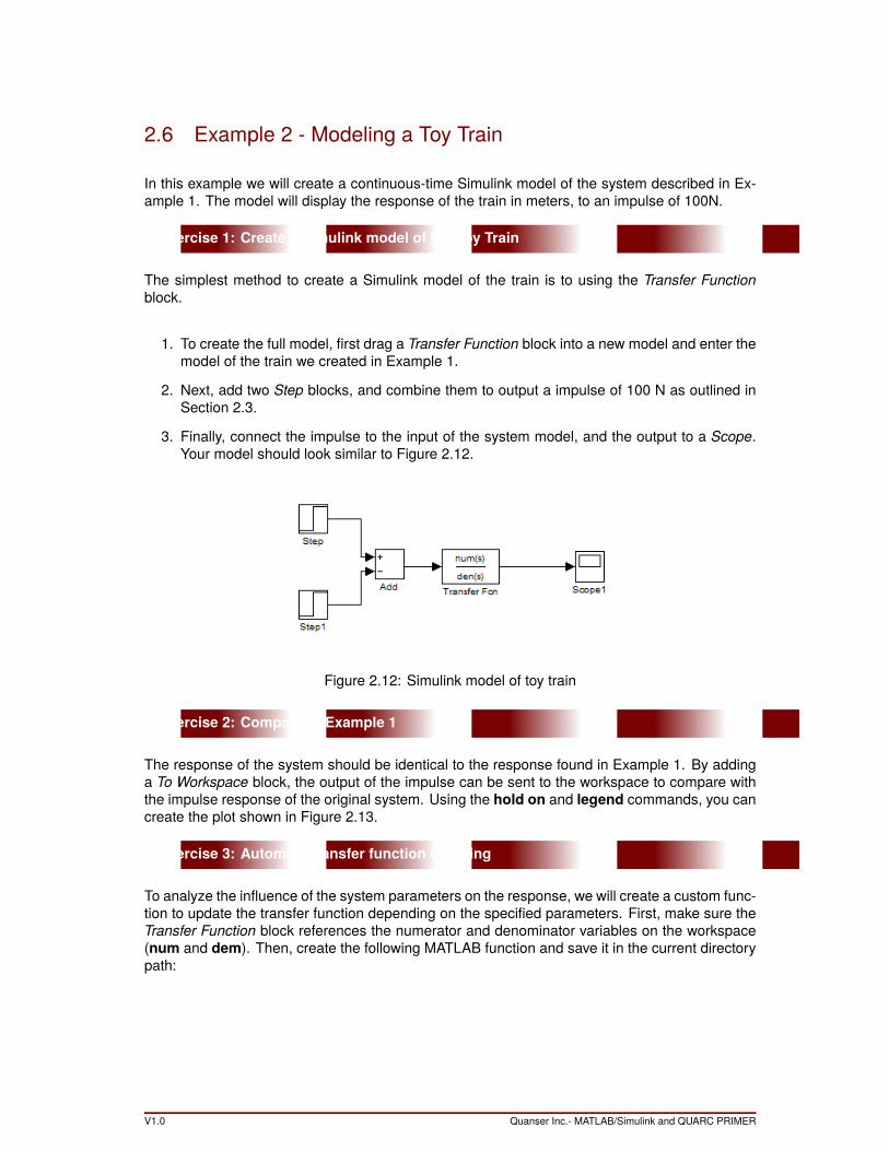
2.6 Example 2 - Modeling a Toy Train

In this example we will create a continuous-time Simulink model of the system described in Ex-ample 1. The model will display the response of the train in meters, to an impulse of 100N.

Exercise 1: Create a Simulink model of the Toy Train

The simplest method to create a Simulink model of the train is to using the Transfer Functionblock.

1. To create the full model, first drag a Transfer Function block into a new model and enter themodel of the train we created in Example 1.

2. Next, add two Step blocks, and combine them to output a impulse of 100 N as outlined inSection 2.3.

3. Finally, connect the impulse to the input of the system model, and the output to a Scope.Your model should look similar to Figure 2.12.

Figure 2.12: Simulink model of toy train

Exercise 2: Compare to Example 1

The response of the system should be identical to the response found in Example 1. By addinga To Workspace block, the output of the impulse can be sent to the workspace to compare withthe impulse response of the original system. Using the hold on and legend commands, you cancreate the plot shown in Figure 2.13.

Exercise 3: Automate transfer function updating

To analyze the influence of the system parameters on the response, we will create a custom func-tion to update the transfer function depending on the specified parameters. First, make sure theTransfer Function block references the numerator and denominator variables on the workspace(num and dem). Then, create the following MATLAB function and save it in the current directorypath:


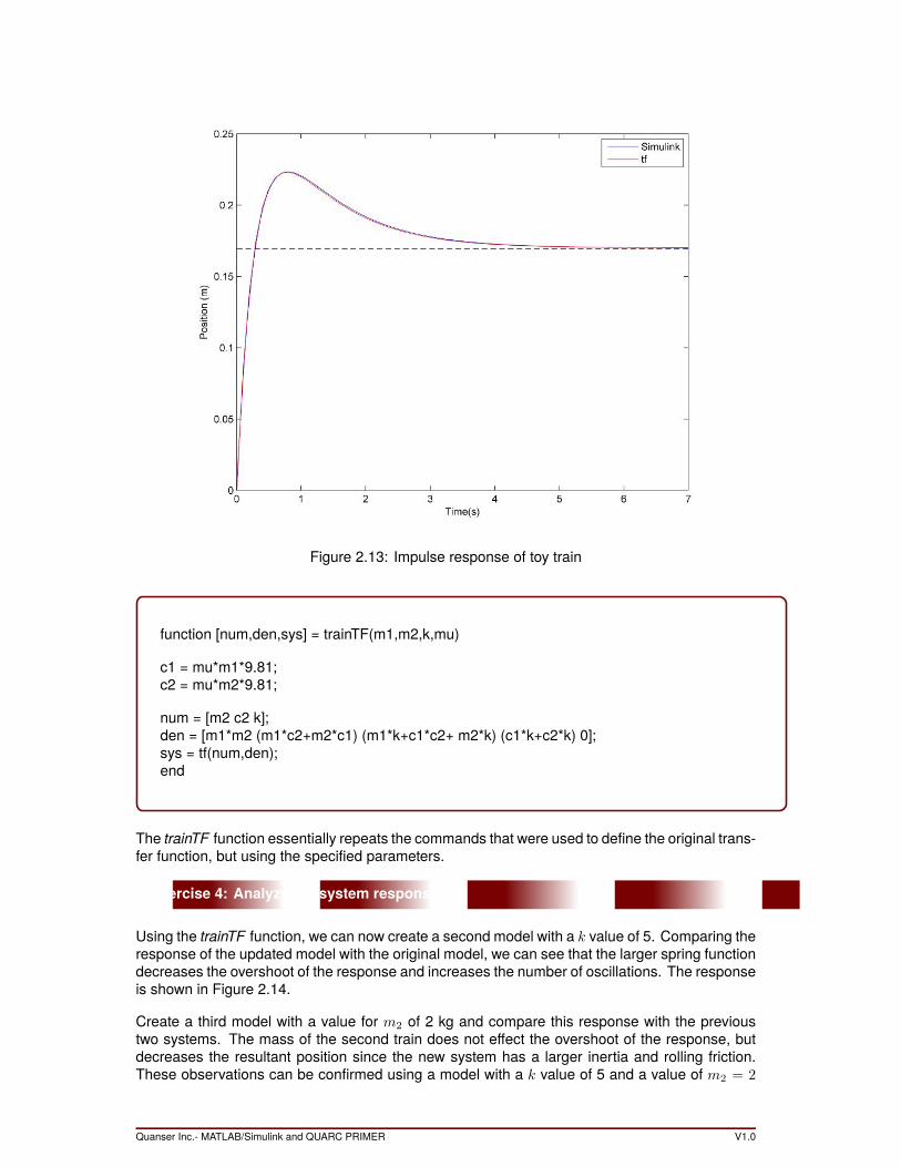
Figure 2.13: Impulse response of toy train

function [num,den,sys] = trainTF(m1,m2,k,mu)

c1 = mu*m1*9.81;c2 = mu*m2*9.81;

num = [m2 c2 k];den = [m1*m2 (m1*c2+m2*c1) (m1*k+c1*c2+ m2*k) (c1*k+c2*k) 0];sys = tf(num,den);end

The trainTF function essentially repeats the commands that were used to define the original trans-fer function, but using the specified parameters.

Exercise 4: Analyze the system response

Using the trainTF function, we can now create a second model with a k value of 5. Comparing theresponse of the updated model with the original model, we can see that the larger spring functiondecreases the overshoot of the response and increases the number of oscillations. The responseis shown in Figure 2.14.

Create a third model with a value for m2 of 2 kg and compare this response with the previoustwo systems. The mass of the second train does not effect the overshoot of the response, butdecreases the resultant position since the new system has a larger inertia and rolling friction.These observations can be confirmed using a model with a k value of 5 and a value of m2 = 2


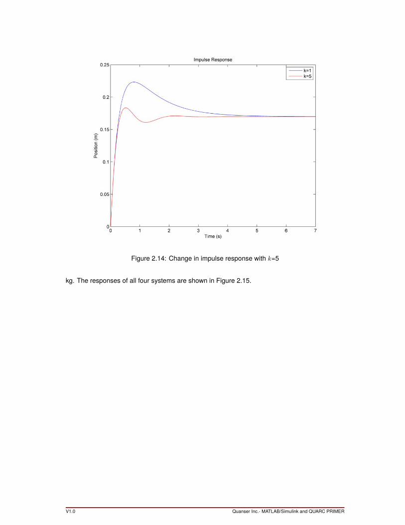
Figure 2.14: Change in impulse response with k=5

kg. The responses of all four systems are shown in Figure 2.15.


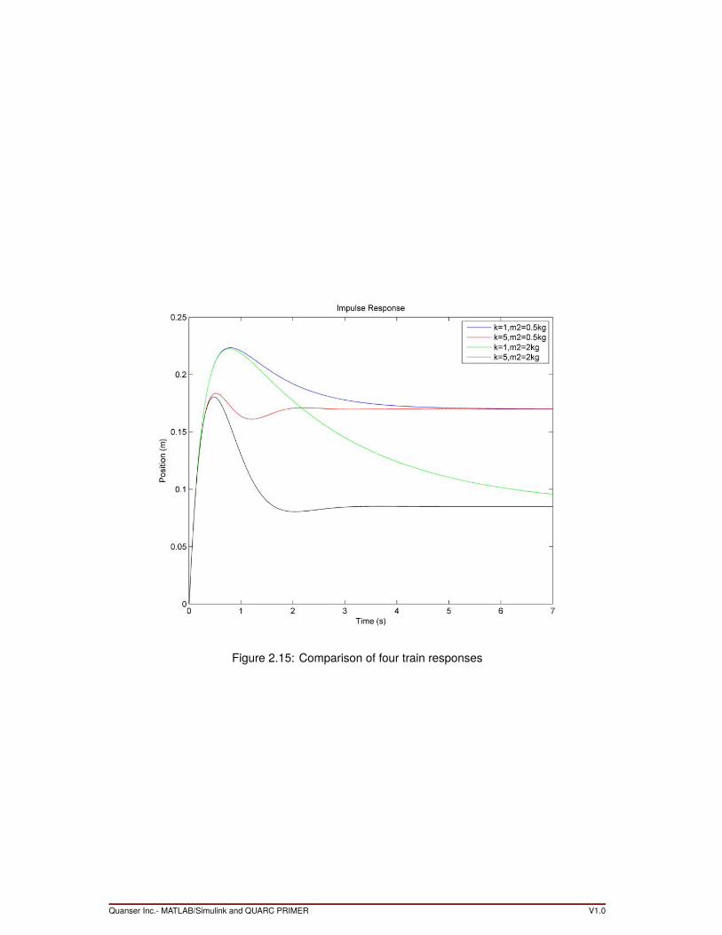
Figure 2.15: Comparison of four train responses


2.7 Example 3 - Creating an Electric Toy Train

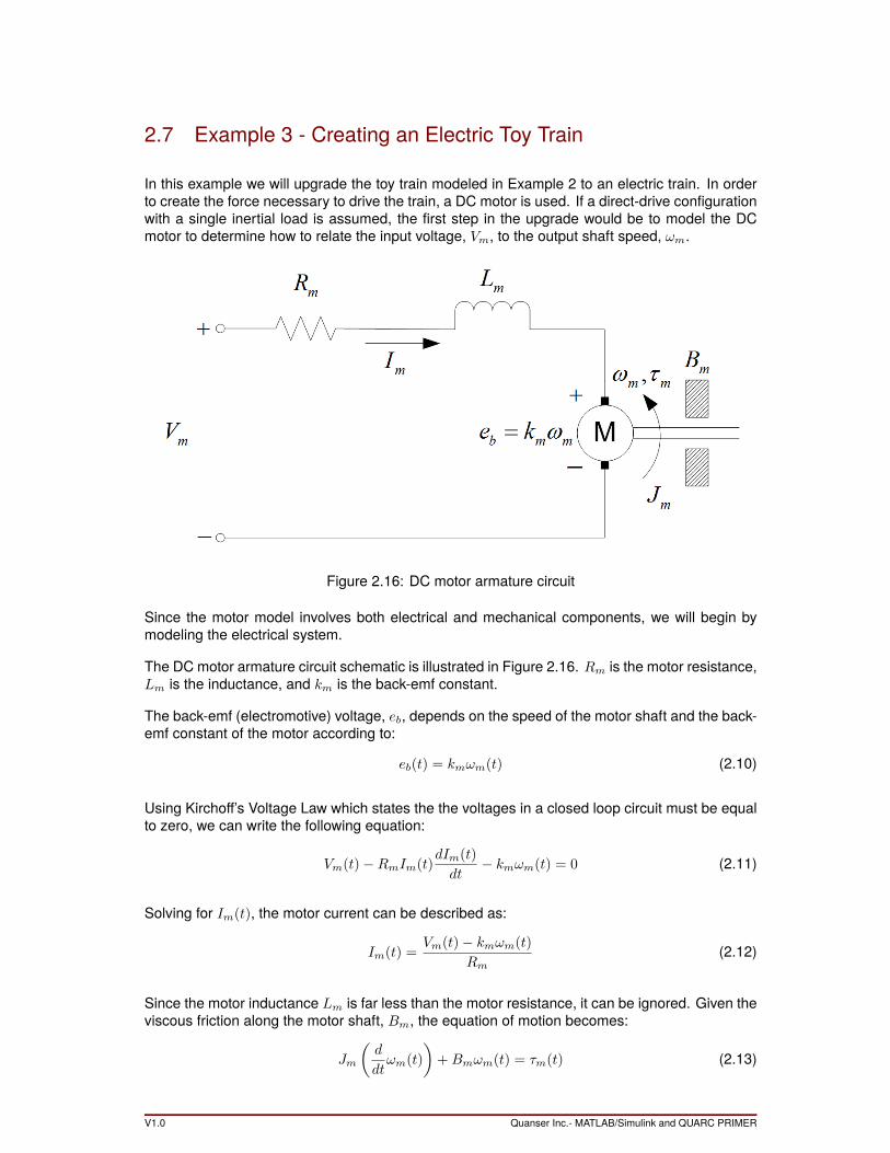
In this example we will upgrade the toy train modeled in Example 2 to an electric train. In orderto create the force necessary to drive the train, a DC motor is used. If a direct-drive configurationwith a single inertial load is assumed, the first step in the upgrade would be to model the DCmotor to determine how to relate the input voltage, Vm, to the output shaft speed, ωm.

Figure 2.16: DC motor armature circuit

Since the motor model involves both electrical and mechanical components, we will begin bymodeling the electrical system.

The DC motor armature circuit schematic is illustrated in Figure 2.16. Rm is the motor resistance,Lm is the inductance, and km is the back-emf constant.

The back-emf (electromotive) voltage, eb, depends on the speed of the motor shaft and the back-emf constant of the motor according to:

eb(t) = kmωm(t) (2.10)

Using Kirchoff’s Voltage Law which states the the voltages in a closed loop circuit must be equalto zero, we can write the following equation:

Vm(t)−RmIm(t)dIm(t)

dt− kmωm(t) = 0 (2.11)

Solving for Im(t), the motor current can be described as:

Im(t) =Vm(t)− kmωm(t)

Rm(2.12)

Since the motor inductance Lm is far less than the motor resistance, it can be ignored. Given theviscous friction along the motor shaft, Bm, the equation of motion becomes:

Jm

(d

dtωm(t)

)+Bmωm(t) = τm(t) (2.13)


where Jm is the moment of inertia of the load and τm is the total torque applied on the load.

The motor torque is proportional to the voltage applied, and is described as:

τm(t) = ηmktIm(t) (2.14)

where kt is the current-torque constant (N.m/A), ηm is themotor efficiency, and Im is the armaturecurrent.

We can express the motor torque with respect to the input voltage Vm(t) and load shaft speedωl(t) by substituting the motor armature current given by Equation 2.12 into the current-torquerelationship:

τm(t) =ηmkt (Vm(t)− kmωm(t))

Rm(2.15)

Now that we have the motor torque expressed as a function of the input voltage, we substituteEquation 2.15 into the equation of motion Equation 2.13:

Jm

(d

dtωm(t)

)+Bmωm(t) =

ηmkt (Vm(t)− kmωm(t))

Rm(2.16)

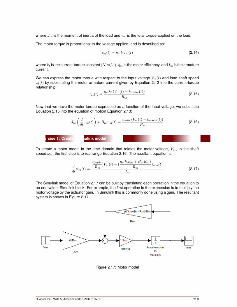
Exercise 1: Create a Simulink model

To create a motor model in the time domain that relates the motor voltage, Vm, to the shaftspeed,ωm, the first step is to rearrange Equation 2.16. The resultant equation is:

d

dtwm(t) =

(ηmktRm

)Vm(t)− (ηmktkm +BmRm)

Rm)ωm(t)

Jm(2.17)

The Simulink model of Equation 2.17 can be built by translating each operation in the equation toan equivalent Simulink block. For example, the first operation in the expression is to multiply themotor voltage by the actuator gain. In Simulink this is commonly done using a gain. The resultantsystem is shown in Figure 2.17.

Figure 2.17: Motor model


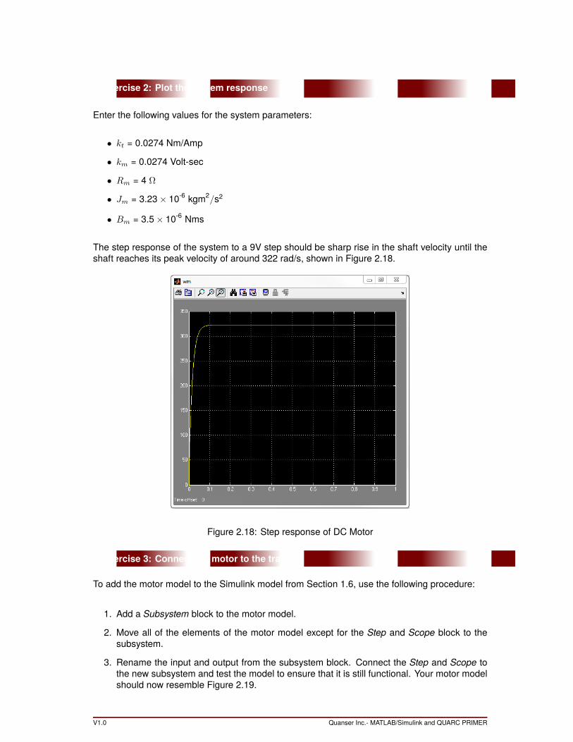
Exercise 2: Plot the system response

Enter the following values for the system parameters:

• kt = 0.0274 Nm/Amp

• km = 0.0274 Volt-sec

• Rm = 4 Ω

• Jm = 3.23× 10-6 kgm2/s2

• Bm = 3.5× 10-6 Nms

The step response of the system to a 9V step should be sharp rise in the shaft velocity until theshaft reaches its peak velocity of around 322 rad/s, shown in Figure 2.18.

Figure 2.18: Step response of DC Motor

Exercise 3: Connect the motor to the train

To add the motor model to the Simulink model from Section 1.6, use the following procedure:

1. Add a Subsystem block to the motor model.

2. Move all of the elements of the motor model except for the Step and Scope block to thesubsystem.

3. Rename the input and output from the subsystem block. Connect the Step and Scope tothe new subsystem and test the model to ensure that it is still functional. Your motor modelshould now resemble Figure 2.19.


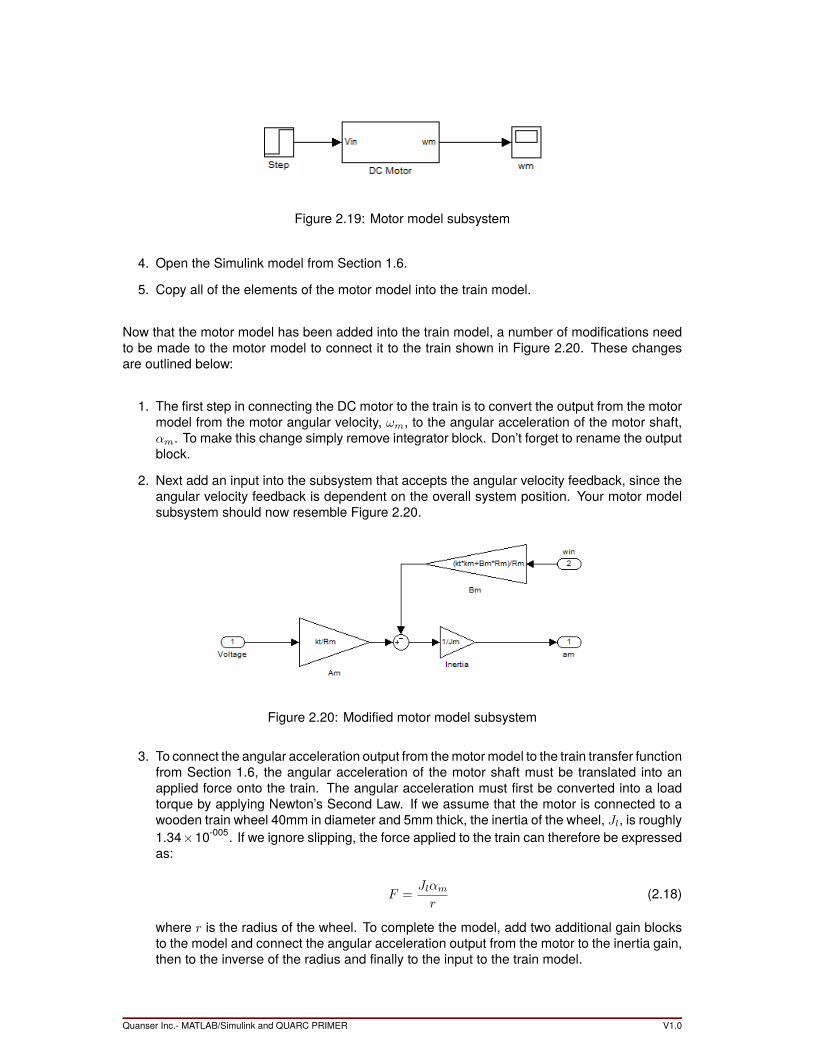
Figure 2.19: Motor model subsystem

4. Open the Simulink model from Section 1.6.

5. Copy all of the elements of the motor model into the train model.

Now that the motor model has been added into the train model, a number of modifications needto be made to the motor model to connect it to the train shown in Figure 2.20. These changesare outlined below:

1. The first step in connecting the DC motor to the train is to convert the output from the motormodel from the motor angular velocity, ωm, to the angular acceleration of the motor shaft,αm. To make this change simply remove integrator block. Don’t forget to rename the outputblock.

2. Next add an input into the subsystem that accepts the angular velocity feedback, since theangular velocity feedback is dependent on the overall system position. Your motor modelsubsystem should now resemble Figure 2.20.

Figure 2.20: Modified motor model subsystem

3. To connect the angular acceleration output from themotormodel to the train transfer functionfrom Section 1.6, the angular acceleration of the motor shaft must be translated into anapplied force onto the train. The angular acceleration must first be converted into a loadtorque by applying Newton’s Second Law. If we assume that the motor is connected to awooden train wheel 40mm in diameter and 5mm thick, the inertia of the wheel, Jl, is roughly1.34×10-005. If we ignore slipping, the force applied to the train can therefore be expressedas:

F =Jlαmr

(2.18)

where r is the radius of the wheel. To complete the model, add two additional gain blocksto the model and connect the angular acceleration output from the motor to the inertia gain,then to the inverse of the radius and finally to the input to the train model.


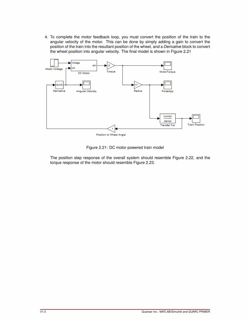
4. To complete the motor feedback loop, you must convert the position of the train to theangular velocity of the motor. This can be done by simply adding a gain to convert theposition of the train into the resultant position of the wheel, and a Derivative block to convertthe wheel position into angular velocity. The final model is shown in Figure 2.21

Figure 2.21: DC motor powered train model

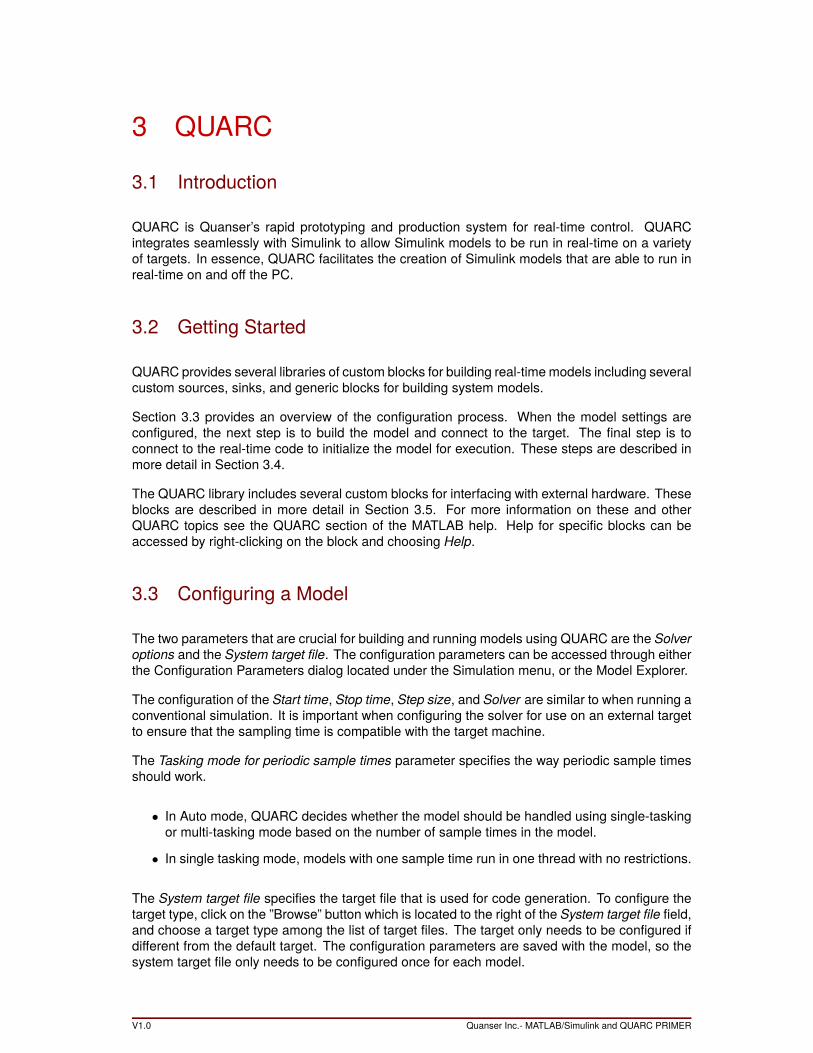
The position step response of the overall system should resemble Figure 2.22, and thetorque response of the motor should resemble Figure 2.23.


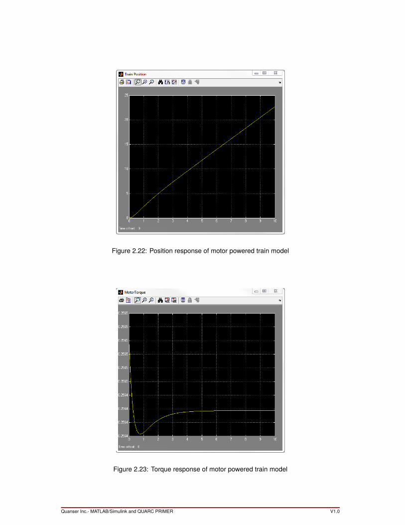
Figure 2.22: Position response of motor powered train model

Figure 2.23: Torque response of motor powered train model


3 QUARC

3.1 Introduction

QUARC is Quanser’s rapid prototyping and production system for real-time control. QUARCintegrates seamlessly with Simulink to allow Simulink models to be run in real-time on a varietyof targets. In essence, QUARC facilitates the creation of Simulink models that are able to run inreal-time on and off the PC.

3.2 Getting Started

QUARC provides several libraries of custom blocks for building real-time models including severalcustom sources, sinks, and generic blocks for building system models.

Section 3.3 provides an overview of the configuration process. When the model settings areconfigured, the next step is to build the model and connect to the target. The final step is toconnect to the real-time code to initialize the model for execution. These steps are described inmore detail in Section 3.4.

The QUARC library includes several custom blocks for interfacing with external hardware. Theseblocks are described in more detail in Section 3.5. For more information on these and otherQUARC topics see the QUARC section of the MATLAB help. Help for specific blocks can beaccessed by right-clicking on the block and choosing Help.

3.3 Configuring a Model

The two parameters that are crucial for building and running models using QUARC are the Solveroptions and the System target file. The configuration parameters can be accessed through eitherthe Configuration Parameters dialog located under the Simulation menu, or the Model Explorer.

The configuration of the Start time, Stop time, Step size, and Solver are similar to when running aconventional simulation. It is important when configuring the solver for use on an external targetto ensure that the sampling time is compatible with the target machine.

The Tasking mode for periodic sample times parameter specifies the way periodic sample timesshould work.

• In Auto mode, QUARC decides whether the model should be handled using single-taskingor multi-tasking mode based on the number of sample times in the model.

• In single tasking mode, models with one sample time run in one thread with no restrictions.

The System target file specifies the target file that is used for code generation. To configure thetarget type, click on the ”Browse” button which is located to the right of the System target file field,and choose a target type among the list of target files. The target only needs to be configured ifdifferent from the default target. The configuration parameters are saved with the model, so thesystem target file only needs to be configured once for each model.


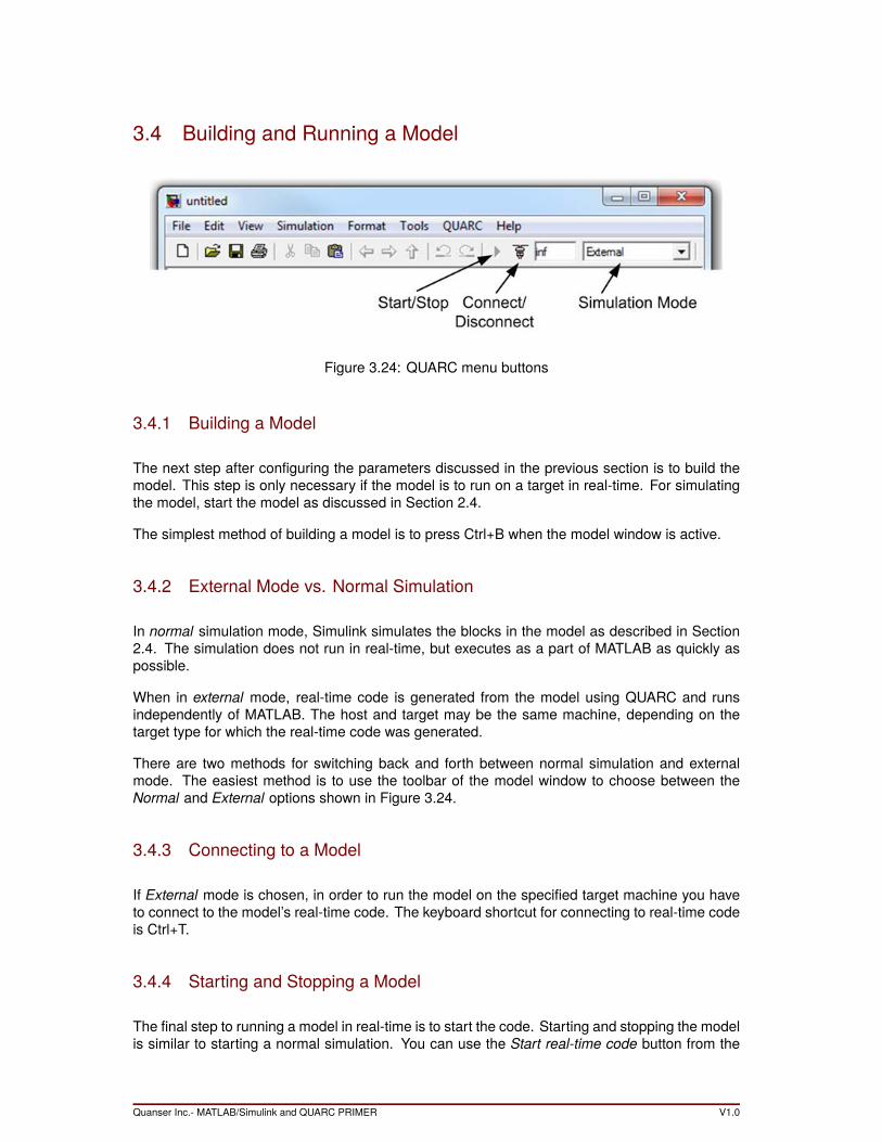
3.4 Building and Running a Model

Figure 3.24: QUARC menu buttons

3.4.1 Building a Model

The next step after configuring the parameters discussed in the previous section is to build themodel. This step is only necessary if the model is to run on a target in real-time. For simulatingthe model, start the model as discussed in Section 2.4.

The simplest method of building a model is to press Ctrl+B when the model window is active.

3.4.2 External Mode vs. Normal Simulation

In normal simulation mode, Simulink simulates the blocks in the model as described in Section2.4. The simulation does not run in real-time, but executes as a part of MATLAB as quickly aspossible.

When in external mode, real-time code is generated from the model using QUARC and runsindependently of MATLAB. The host and target may be the same machine, depending on thetarget type for which the real-time code was generated.

There are two methods for switching back and forth between normal simulation and externalmode. The easiest method is to use the toolbar of the model window to choose between theNormal and External options shown in Figure 3.24.

3.4.3 Connecting to a Model

If External mode is chosen, in order to run the model on the specified target machine you haveto connect to the model’s real-time code. The keyboard shortcut for connecting to real-time codeis Ctrl+T.

3.4.4 Starting and Stopping a Model

The final step to running a model in real-time is to start the code. Starting and stopping the modelis similar to starting a normal simulation. You can use the Start real-time code button from the


toolbar. Similarly, to stop the model you can use the Stop real-time code button on the toolbar, oryou can press the Pause key.

3.5 Accessing Hardware

QUARC supports a variety of data acquisition cards, includingQuanser’s ownQ4 andQ8Hardware-in-the-Loop (HIL) boards, the National Instruments PCI-6259 and many more. Hardware con-nected to these boards can be accessed by simply placing the appropriate blocks in your Simulinkdiagram. The blocks are found in the library browser under QUARC Targets | Data Acquisition| Generic and require very little additional configuration. Please consult the Using HardwareQUARC demos for more examples of the HIL blocks.

3.5.1 HIL Initialize Block

This block can be found in the Simulink Library Browser under the QUARC Targets | Data Acqui-sition | Generic | Configuration and should be placed in all models that require hardware accessof some type. The HIL Initialize block associates a board name with a particular HIL board. Thename assigned to each board will appear in the list of boards for every other HIL block in thediagram.

An important function of the HIL Initialize block is to configure the I/O on the card. For exam-ple, many cards allow the digital I/O lines to be programmed as inputs or outputs. The DigitalInputs and Digital Outputs tabs are used to configure which digital I/O lines are inputs and out-puts respectively. Similarly, many cards permit the range of the analog inputs and outputs tobe programmed. The Analog Inputs and Analog Outputs tabs are used for this purpose. Manyother features of data acquisition cards are configured using the tabs of the HIL Initialize block.Be sure to check the settings on each tab carefully to ensure that your card is set up properly.Please consult the HIL Initialize help page for full details.

3.5.2 Immediate I/O HIL Blocks

These blocks are found in the Simulink Library Browser under the QUARC Targets | Data Ac-quisition | Generic | Immediate I/O. The immediate I/O blocks read from or write to the specifiedchannels every time the block is executed. The channels are read from or written to immediately.

3.5.3 Buffered I/O HIL Blocks

These blocks are found in the Simulink Library Browser under QUARC Targets | Data Acquisition| Generic | Buffered I/O. The buffered I/O blocks can be used to read in buffered data. This can bedone by specifying the number of samples to be buffered (buffer size) in the dialog box associatedwith the block. The specified number of samples are then read at the given sampling rate andbuffered. These values are output from the block once all the samples have been read.


3.5.4 Timebase HIL Blocks

These blocks are found in the Simulink Library Browser under QUARC Targets | Data Acquisition |Generic | Timebases. The hardware timebase blocks read from or write to the specified channelsat the sampling rate of themodel and act as a timebase for themodel. More specifically, wheneverhardware is accessed via the Timebase HIL blocks, acquisition timing and the triggering of themodel execution are done by a hardware timer on the DAQ (for better performance) rather thanthe target OS (e.g. Windows) system timebase.

3.6 Example 4 - Position Controlled Toy Train

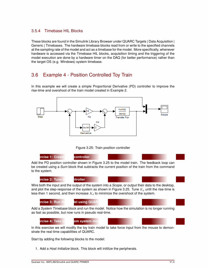
In this example we will create a simple Proportional Derivative (PD) controller to improve therise-time and overshoot of the train model created in Example 2.

Figure 3.25: Train position controller

Exercise 1: Create a PD controllerAdd the PD position controller shown in Figure 3.25 to the model train. The feedback loop canbe created using a Sum block that subtracts the current position of the train from the commandto the system.

Exercise 2: Tune the ControllerWire both the input and the output of the system into a Scope, or output their data to the desktop,and plot the step-response of the system as shown in Figure 3.25. Tune Kp until the rise-time isless-then 1 second, and then increase Kd to minimize the overshoot of the system.

Exercise 3: Run the model using QUARC

Add a System Timebase block and run the model. Notice how the simulation is no longer runningas fast as possible, but now runs in pseudo real-time.

Exercise 4: Take input from system mouse

In this exercise we will modify the toy train model to take force input from the mouse to demon-strate the real-time capabilities of QUARC.

Start by adding the following blocks to the model:

1. Add a Host Initialize block. This block will initilize the peripherals.


Figure 3.26: Train step response

2. Add a Host Mouse block from the Host library located in QUARC Targets | Devices | Pe-ripherals | Host. This block will interface with the system mouse.

3. From the same library, add a Host Keyboard block. This blocks will access the status of akey on the keyboard.

4. Add a Switch from the Commonly Used Blocks library.

5. Add a Signal Generator from the Sources library.

Wire the new blocks as shown in Figure 3.27.

Configure the new blocks as follows:

1. Open the Host Initialize block properties and note the name of the host.

2. In the Host Keyboard block properties, choose a key to serve as the switch input (e.g. F1).

3. Open the Host Mouse block properties and enter the host name from the drop menu.

4. Configure the Signal Generator block to output a square-wave with an amplitude of 1 andfrequency of 0.5.

When you run the system model, the scope should show the response of the system to the pulsetrain output by the Signal Generator. When the key specified in the Host Keyboard is pressed, thesystem should match the position of the mouse y-axis in real-time. Play with the mouse positionand observe the system response.


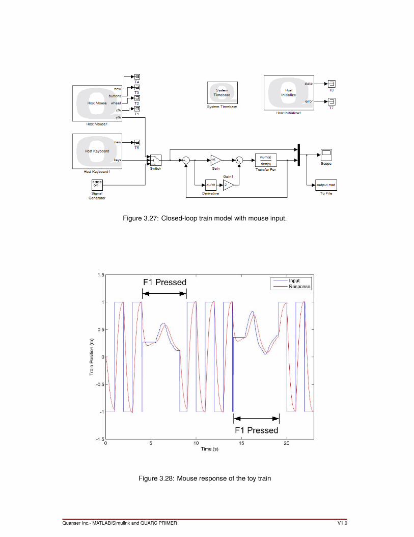
Figure 3.27: Closed-loop train model with mouse input.

Figure 3.28: Mouse response of the toy train


4 MATLABCheat Sheet& : AND‖ : OR: NOT= : Not equal< : Less than<= : Less than or equal== : Equal> : Greater than>= : Greater than or equalabs: Absolute valueangle: Returns phase angle(s) of complex number(s)axis: Set the scales of the current plot’b’: bluebode: Draw a Bode plot’c’: cyanc2d: Convert continuous to discrete modelceil: Round to the nearest integer toward∞char: Creates character arrayclf: Clear figureclose all: Close all figuresclose: Close current figureconj: Complex conjugateconv: Convolutioncross: Cross productctrb: Controllability matrixdeconv: Deconvolutiondet: Determinantdlqr: Linear-Quadratic Requlator for discrete-time sys-temdlsim: Simulation of discrete-time linear systemdot: Dot productdstep: Step response of discrete-time linear systemeig: Eigenvalues of a matrixexp: Exponentialeye: Identity matrixfeedback: Feedback interconnection of LTI systemsfigure: Create a new figurefind: Finds indices of specific valuesfindstr: Find a stringfloor: Round to the nearest integer toward -∞’g’: greenget: Query graphics object propertieshold: Hold current plotimag: Imaginary part(s) of complex number(s)impulse: Impulse response of continuous-time lin-ear systeminput: Prompt for user inputinv: Matrix inverseisempty: True if matrix is empty’k’ : blacklegend: Graph legendlinspace: Returns a linearly spaced vectorlog: Natural logarithmlog10: Common (base-10) logarithmloglog: Plot using log-log scale

logspace: Return a logarithmically spaced vectorlqr: Linear-Quadratic Regulator for continuous sys-temlsim: Simulate LTI model response’m’ : Magentamag2db: Convert magnitude to decibels (dB)margin: Find gainmargin, phasemargin, and crossoverfrequenciesmean: Averagemedian: Mediannorm: Norm of a vectornyquist: Draw a Nyquist plotobsv: The observability matrixones: Create a vector or matrix of onesplace: Compute gains to place poles of x = Ax+buplot: Draw a plotpoly: Find characteristic polynomialpolyadd: Add two polynomialspolyfit: Fit a polynomial to datapolyval: Polynomial evaluation’r’ : Redrand: Generate random number between 0 and 1rank: Find the number of linearly independent rowsor columns of a matrixreal: Real part of a complex numberrlocus: Draw root locusroots: Find the roots of a polynomialround: Round toward the nearest integer.series: Series interconnection of LTI systemsset: Set graphics object propertiessize: Dimension of a vector or matrixsort: Sorts columnssqrt: Square rootss: Create state-space modelss2tf: State-space to transfer functionss2zp: State-space to pole-zerostd: Calculate the standard deviationstep: Plot step responsestrcmp: Compare stringssubplot: Create multiple plots in figuresum: Sum columnstf: Create transfer functiontf2ss: Convert transfer function to state-spacetf2zp: Convert transfer function to Pole-zerotitle: Add a title to current plot’w’ : Whitewbw: Bandwidth frequency given the damping ratioand the rise or settling timexlabel: Add label to x-axis’y’ : Yellowylabel: Add text label to y-axiszeros: Create a vector or matrix of zeroszp2ss: Pole-zero to state-spacezp2tf: Pole-zero to transfer function


Appendix A

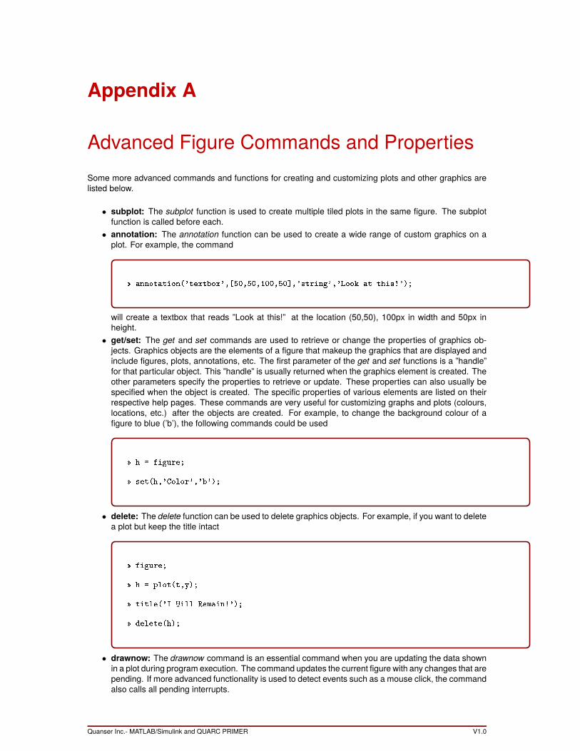
Advanced Figure Commands and PropertiesSome more advanced commands and functions for creating and customizing plots and other graphics arelisted below.

• subplot: The subplot function is used to create multiple tiled plots in the same figure. The subplotfunction is called before each.

• annotation: The annotation function can be used to create a wide range of custom graphics on aplot. For example, the command

annotation('textbox',[50,50,100,50],'string','Look at this!');

will create a textbox that reads ”Look at this!” at the location (50,50), 100px in width and 50px inheight.

• get/set: The get and set commands are used to retrieve or change the properties of graphics ob-jects. Graphics objects are the elements of a figure that makeup the graphics that are displayed andinclude figures, plots, annotations, etc. The first parameter of the get and set functions is a ”handle”for that particular object. This ”handle” is usually returned when the graphics element is created. Theother parameters specify the properties to retrieve or update. These properties can also usually bespecified when the object is created. The specific properties of various elements are listed on theirrespective help pages. These commands are very useful for customizing graphs and plots (colours,locations, etc.) after the objects are created. For example, to change the background colour of afigure to blue (’b’), the following commands could be used

h = figure;

set(h,'Color','b');

• delete: The delete function can be used to delete graphics objects. For example, if you want to deletea plot but keep the title intact

figure;

h = plot(t,y);

title('I Will Remain!');

delete(h);

• drawnow: The drawnow command is an essential command when you are updating the data shownin a plot during program execution. The command updates the current figure with any changes that arepending. If more advanced functionality is used to detect events such as a mouse click, the commandalso calls all pending interrupts.


Appendix B

Additional Programming ConceptsB.0.1 Data Structures

The MATLAB environment includes several classes, or data types, to accommodate various data types orstorage requirements. The more basic numeric classes have already been addressed and include booleanvalues, numeric arrays, character arrays, and function handles. The other type of class that is available inMATLAB is referred to as a heterogeneous container, meaning it can hold a variety of data types together.There are two types of containers: structures and cell arrays.

• StructuresStructures in MATLAB provide a means to store different types of data together in a single entity.Structures consist of data arrays and fields, which serve as a label for the individual datasets. Withineach field, data arrays can be any type and valid array dimension. Structures not only facilitate moreorganized data storage, but also enable users to pass multiple datasets to and from functions.To declare a structure the command struct is invoked, followed by the contents of the structure. Forexample, the following statement creates a structure containing a scalar, a numeric array, and a char-acter array:

data = struct('Name','John','Age',32,'Times',[10.56,9.42,8.35,11.55]);

To access the contents of the structure, the period ”.” is used to ”index” into the structure as follows

data.Name

Output:

ans =

John

Arrays of structures can also be created by assigning the last index in an array to the structure. Thearray elements are automatically populated with the ”default” fields used in the declaration. For ex-ample, to create an array of the structures declared earlier you could enter


dataset(5) = data

Output:

dataset =

1x5 struct array with fields:

Name

Age

Times

Structures can also be nested within one another by declaring a structure, and then including it in afield of a parent structure. For example, the following statement includes the structure ”student” in theparent structure ”classroom”

student = struct('Name','Arya','Age','13','Marks',[87,92,88,78,81]);

classroom = struct('Number',201,'Teacher','Mrs. Stark','Students',student);

Output:

classroom =

Number: 201

Teacher: 'Mrs. Stark'

Students: [1x1 struct]

classroom.Student

ans =

Name: 'Arya'

Age: '13'

Marks: [87 92 88 78 81]

• Cell ArraysA cell array is an array of containers called cells in which you can store different types of data. A cellarray is similar to a structure in that it contains different datatypes divided into separate containers,but uses a traditional array structure rather than fields to arrange the data. Cell arrays are created inmuch the same manner as creating any other array in MATLAB, but using curly braces , instead ofsquare. For example to create a cell array of character and numeric arrays you might use the followingstatements

car = 'Aston Martin','DB9',[469,443,3880,4.6,4.8,190];

Output:

car =

'Aston Martin' 'DB9' [1x6 double]

Accessing the cells within the array can be done with either the usual round or curly braces


car 1,2

Outputs:

ans =

'DB9'

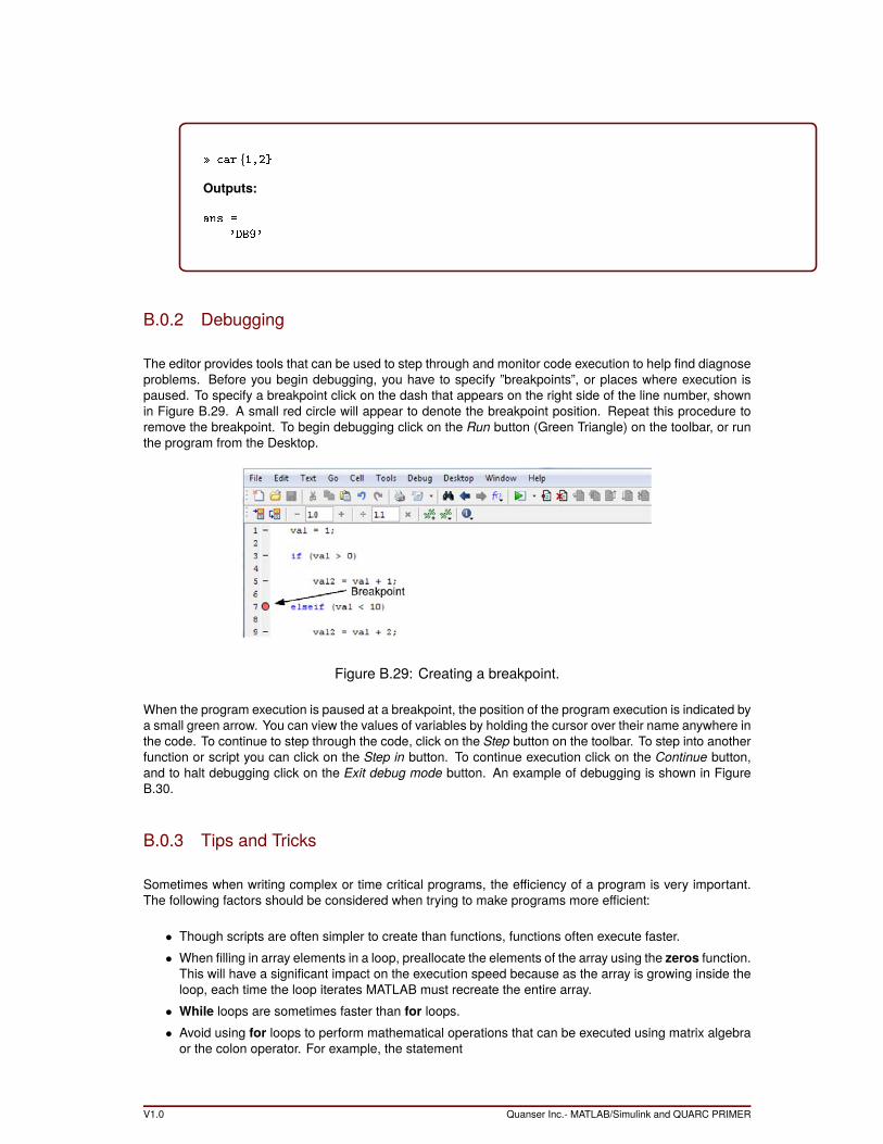
B.0.2 Debugging

The editor provides tools that can be used to step through and monitor code execution to help find diagnoseproblems. Before you begin debugging, you have to specify ”breakpoints”, or places where execution ispaused. To specify a breakpoint click on the dash that appears on the right side of the line number, shownin Figure B.29. A small red circle will appear to denote the breakpoint position. Repeat this procedure toremove the breakpoint. To begin debugging click on the Run button (Green Triangle) on the toolbar, or runthe program from the Desktop.

Figure B.29: Creating a breakpoint.

When the program execution is paused at a breakpoint, the position of the program execution is indicated bya small green arrow. You can view the values of variables by holding the cursor over their name anywhere inthe code. To continue to step through the code, click on the Step button on the toolbar. To step into anotherfunction or script you can click on the Step in button. To continue execution click on the Continue button,and to halt debugging click on the Exit debug mode button. An example of debugging is shown in FigureB.30.

B.0.3 Tips and Tricks

Sometimes when writing complex or time critical programs, the efficiency of a program is very important.The following factors should be considered when trying to make programs more efficient:

• Though scripts are often simpler to create than functions, functions often execute faster.• When filling in array elements in a loop, preallocate the elements of the array using the zeros function.

This will have a significant impact on the execution speed because as the array is growing inside theloop, each time the loop iterates MATLAB must recreate the entire array.

• While loops are sometimes faster than for loops.• Avoid using for loops to perform mathematical operations that can be executed using matrix algebra

or the colon operator. For example, the statement


Figure B.30: Debugging a program.

t = 0:1:100;

y = t2+2*t+1;

is much more efficient than

for t=0:100

y(t) = t2+2*t+1;

end

• Consider using the ”short-circuiting” logical operators && and || when possible. These operatorsavoid evaluating the entire condition if the first statement satisfies the condition. For example, thestatement if(var > 1 && var2 < 10) will continue execution if var <= 1 without checking the value ofvar2.

Some other tricks include:

• The key sequence Ctrl+C will halt execution of any running functions or scripts.• Pressing Tab when entering a command into the CommandWindow will auto-complete the statement

with a list of probable commands.• Pressing the UP arrow at the command prompt will scroll through the previously entered commands.


matlab simulink quarc primer · 2017-03-14 · matlab/simulink and quarc primer [email protected]

Documents