matlab tutorial : root locus - the university ... - … - utah eceece3510/microsoft powerpoint -...
TRANSCRIPT
Matlab Tutorial : Root Locus
ECE 3510
Heather Malko
The University of Utah
Table of Context
� 1.0 Introduction
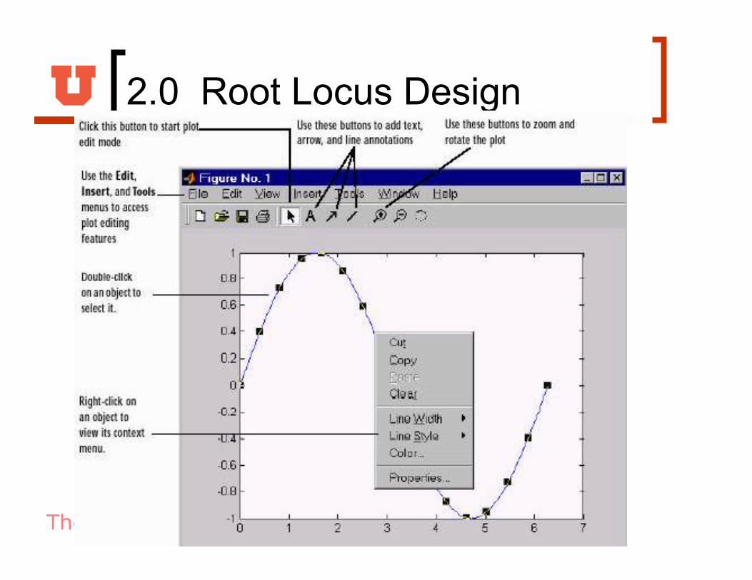
� 2.0 Root Locus Design
� 3.0 SISO Root Locus
� 4.0 GUI for Controls
The University of Utah
1.0 Introduction
� A root loci plot is simply a plot of the s zero values and the s poles on a graph with real and imaginary ordinates.
� The root locus is a curve of the location of the poles of a transfer function as some parameter (generally the gain K) is varied.
� The locus of the roots of the characteristic equation of the closed loop system as the gain varies from zero to infinity gives the name of the method.
� This method is very powerful graphical technique for investigating the effects of the variation of a system parameter on the locations of the closed loop poles.

The University of Utah
1.0 Introduction
� General rules for constructing the root locus exist and if the designer follows them, sketching of the root loci becomes a simple matter.
� Root loci are completed to select the best parameter value for stability.
� A normal interpretation of improving stability is when the real part of a pole is further left of the imaginary axis.

The University of Utah
1.0 Introduction
� Matlab and Root Locus:
� MATLAB Control System Toolbox contains two Root Locus design GUI, sisotool and rltool. These are two interactive design tools of SISO.

The University of Utah
1.0 Introduction
� Matlab’s Useful Commands :
� http://courses.ece.uiuc.edu/ece486/documents/matlab_cmds.html
� http://www-ccs.ucsd.edu/matlab/toolbox/control/refintro.html
� http://users.ece.gatech.edu/~bonnie/book/TUTORIAL/tut_3.html
The University of Utah
2.0 Root Locus Tutorial # 1
� Key Matlab commands used in this tutorial:
cloop, rlocfind, rlocus, sgrid, step
� Matlab commands from the control system
toolbox are highlighted in red.
The University of Utah
2.0 Root Locus Design
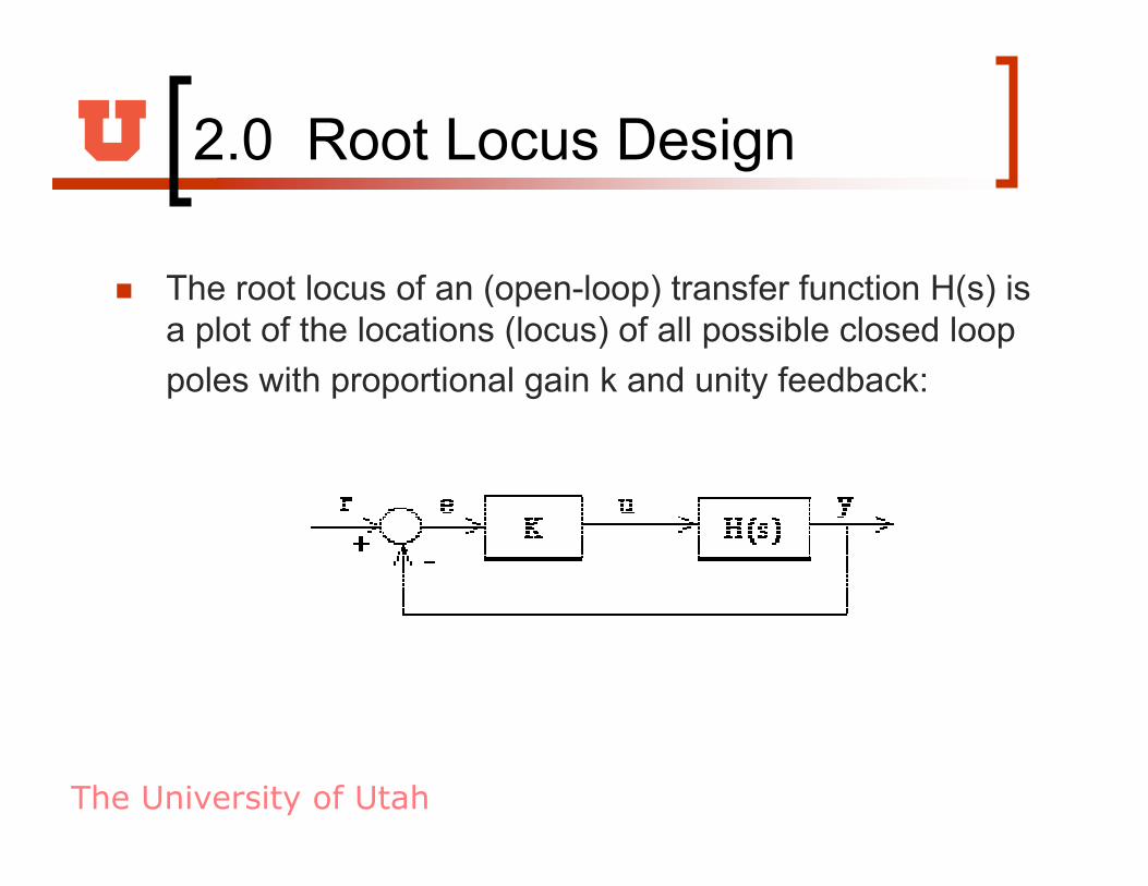
� The root locus of an (open-loop) transfer function H(s) is
a plot of the locations (locus) of all possible closed loop
poles with proportional gain k and unity feedback:

The University of Utah
2.0 Root Locus Design
� The closed-loop transfer function is:
and thus the poles of the closed loop system are values of s such that 1 + K H(s) = 0.
� If H(s) = b(s)/a(s), then this equation has the form:
� Let n = order of a(s) and m = order of b(s) [the order of a polynomial is the highest power of s that appears in it].
The University of Utah
2.0 Root Locus Design
� Consider all positive values of k.
� In the limit as k -> 0, the poles of the closed-loop system
are a(s) = 0 or the poles of H(s).
� In the limit as k -> infinity, the poles of the closed-loop
system are b(s) = 0 or the zeros of H(s).
� No matter what we pick k to be, the closed-loop
system must always have n poles, where n is the
number of poles of H(s). The root locus must have n
branches, each branch starts at a pole of H(s) and
goes to a zero of H(s).

The University of Utah
2.0 Root Locus Design
� Consider an open loop system which has a transfer function of
num=[1 7];
den=conv(conv([1 0],[1 5]),conv([1 15],[1 20])); rlocus(num,den)
axis([-22 3 -15 15])

The University of Utah
2.0 Root Locus Design
-20 -15 -10 -5 0-15
-10
-5
0
5
10
15
Root Locus
Real Axis
Imaginary Axis

The University of Utah
2.0 K from the root locus
� The plot above shows all possible closed-loop pole locations for a pure proportional controller.
� So use the command sgrid(Zeta,Wn) to plot lines of constant damping ratio and natural frequency.
� Its two arguments are the damping ratio (Zeta) and natural frequency (Wn) [these may be vectors if you want to look at a range of acceptable values]. In the problem, an overshoot less than 5% (which means a damping ratio Zeta of greater than 0.7) and a rise time of 1 second (which means a natural frequency Wngreater than 1.8).
The University of Utah
2.0 K from the root locus
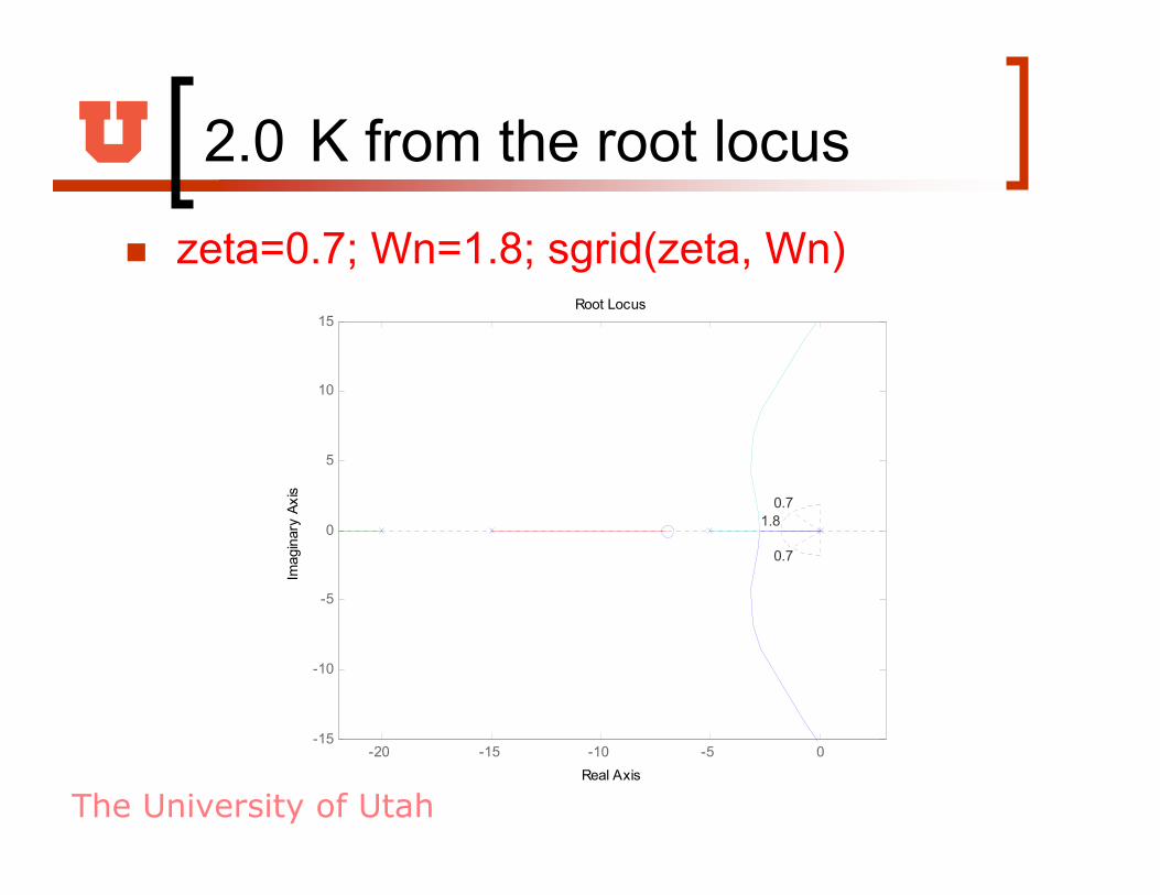
� zeta=0.7; Wn=1.8; sgrid(zeta, Wn)
-20 -15 -10 -5 0-15
-10
-5
0
5
10
15
0.7
0.7
1.8
Root Locus
Real Axis
Imaginary Axis

The University of Utah
2.0 K from the root locus
� The plot above shows all possible closed-loop pole locations for a pure proportional controller.
� So use the command sgrid(Zeta,Wn) to plot lines of constant damping ratio and natural frequency.
� Its two arguments are the damping ratio (Zeta) and natural frequency (Wn) [these may be vectors if you want to look at a range of acceptable values]. In the problem, an overshoot less than 5% (which means a damping ratio Zeta of greater than 0.7) and a rise time of 1 second (which means a natural frequency Wngreater than 1.8).

The University of Utah
2.0 K from the root locus
� [kd,poles] = rlocfind(num,den)
-20 -15 -10 -5 0-15
-10
-5
0
5
10
15
0.7
0.7
1.8
Root Locus
Real Axis
Imaginary Axis

The University of Utah
2.0 K from the root locus
� [kd,poles] = rlocfind(num,den)
� Select a point in the graphics window
� selected_point = -2.6576 + 0.0466i
� kd = 306.9457
� poles =
1) -21.8180
2) -12.5794
3) -2.9373
4) -2.6652
The University of Utah
2.0 Closed-loop response
� In order to find the step response, one needs to know
the closed-loop transfer function. [numCL, denCL] =
cloop((kd)*num, den)
� The two arguments to the function cloop are the
numerator and denominator of the open-loop system.
You need to include the proportional gain that you have
chosen. Unity feedback is assumed.
� If you have a non-unity feedback situation, look at the
help file for the Matlab function feedback, which can find
the closed-loop transfer function with a gain in the
feedback loop.

The University of Utah
2.0 Closed-loop responseL
� [numCL, denCL] = cloop((kd)*num, den)
� numCL = 1.0e+003 * 0 0 0
0.3069 2.1486
� denCL = 1.0e+003 * 0.0010 0.0400
0.4750 1.8069 2.1486
� >> step(numCL,denCL)

The University of Utah
2.0 Closed-loop responseL
0 0.5 1 1.5 2 2.50
0.1
0.2
0.3
0.4
0.5
0.6
0.7
0.8
0.9
1
Step Response
Time (sec)
Amplitude
The University of Utah
2.0 Root Locus Design

The University of Utah
2.0 Root Locus Design
� Reference:
http://www.engin.umich.edu/group/ctm/rlocus
/rlocus.html
� http://www.cs.wright.edu/people/faculty/kratt
an/courses/414/lab1/matlabcommands.pdf

The University of Utah
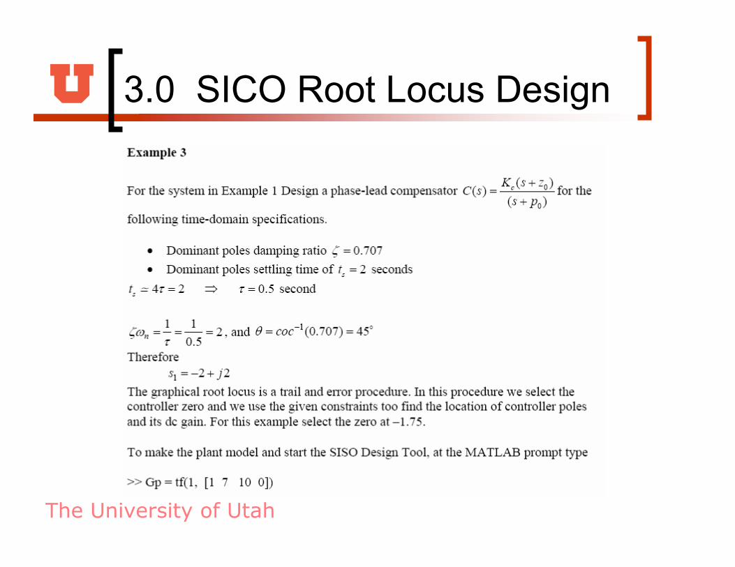
3.0 SICO Root Locus Design
� Design Constraints
� When designing compensators, it is common to have
design specifications that call for specific settling times,
damping ratios, and other characteristics.
� The SISO Design Tool provides design constraints that
can help make the task of meeting design specifications
easier. The New Constraint window, which allows you
to create design constraints, automatically changes to
reflect which constraints are available for the view in
which you are working.

The University of Utah
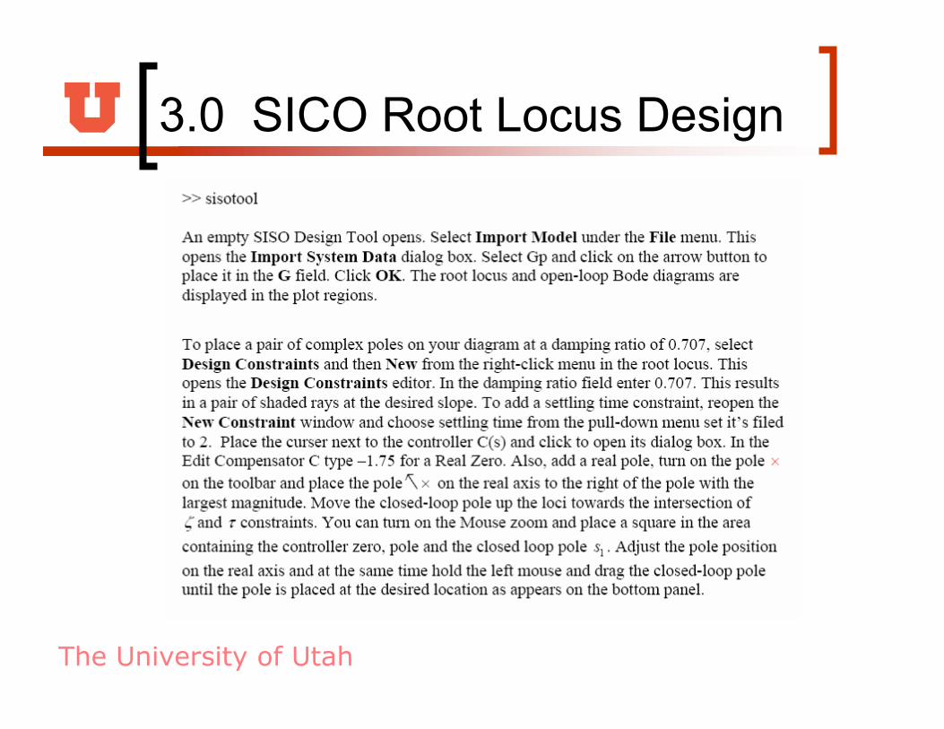
3.0 SICO Root Locus Design
� Design Constraints
� Select Design Constraints and then New to open the
New Constraint window, which is shown below.

The University of Utah
3.0 SICO Root Locus Design
� Design Constraints for the Root Locus
� For the root locus, you have the following constraint
types:
� Settling Time
� Percent Overshoot
� Damping Ratio
� Natural Frequency

The University of Utah
3.0 SICO Root Locus Design
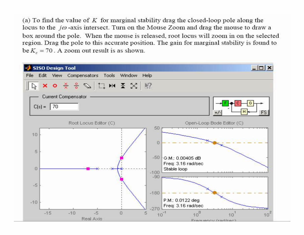
� Settling Time. If you specify a settling time in the
continuous-time root locus, a vertical line appears on
the root locus plot at the pole locations associated with
the value provided (using a first-order approximation). In
the discrete-time case, the constraint is a curved line.
� Percent Overshoot. Specifying percent overshoot in
the continuous-time root locus causes two rays, starting
at the root locus origin, to appear. These rays are the
locus of poles associated with the percent value (using
a second-order approximation). In the discrete-time
case, In the discrete-time case, the constraint appears
as two curves originating at (1,0) and meeting on the
real axis in the left-hand plane.
The University of Utah
3.0 SICO Root Locus Design
� Damping Ratio. Specifying a damping ratio in the
continuous-time root locus causes two rays, starting at
the root locus origin, to appear. These rays are the
locus of poles associated with the damping ratio. In the
discrete-time case, the constraint appears as curved
lines originating at (1,0) and meeting on the real axis in
the left-hand plane.
� Natural Frequency. If you specify a natural frequency,
a semicircle centered around the root locus origin
appears. The radius equals the natural frequency.
The University of Utah
3.0 SICO Root Locus Design
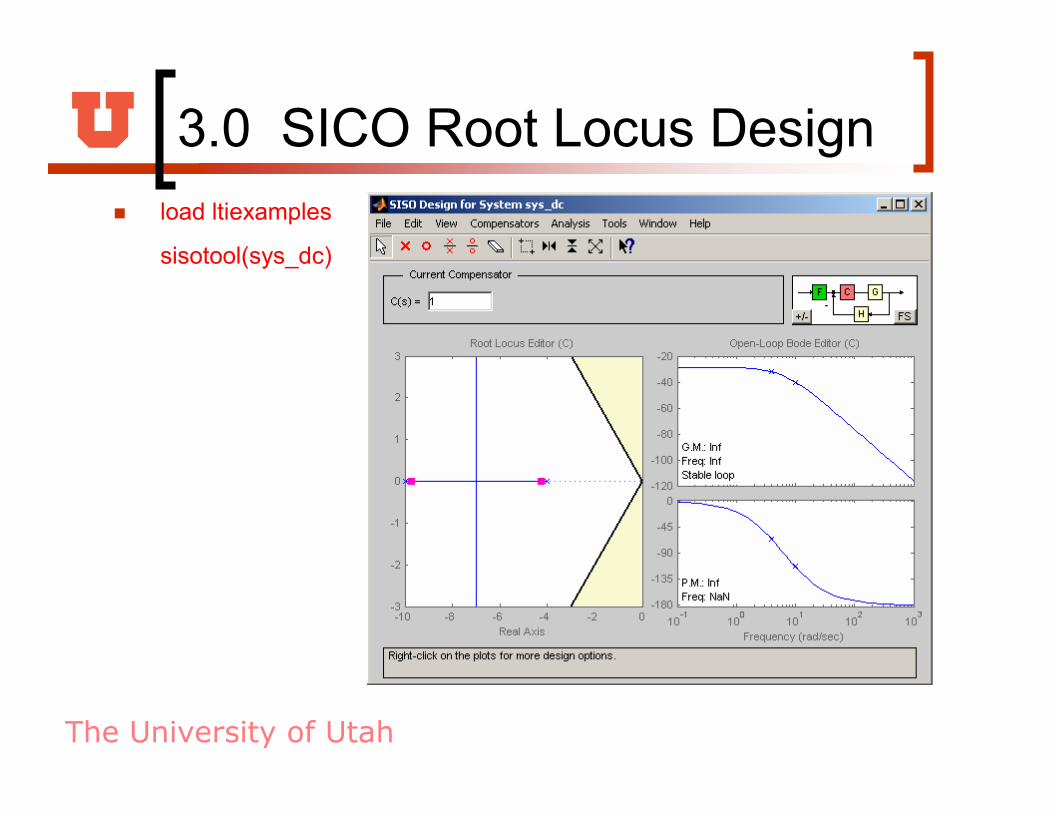
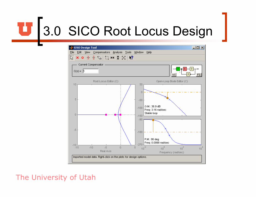
� load ltiexamples
sisotool(sys_dc)

The University of Utah
3.0 SICO Root Locus Design
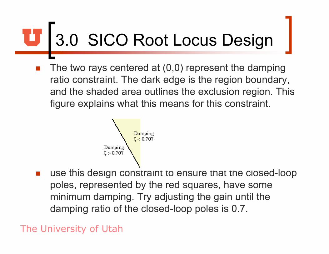
� The two rays centered at (0,0) represent the damping
ratio constraint. The dark edge is the region boundary,
and the shaded area outlines the exclusion region. This
figure explains what this means for this constraint.
� use this design constraint to ensure that the closed-loop
poles, represented by the red squares, have some
minimum damping. Try adjusting the gain until the
damping ratio of the closed-loop poles is 0.7.
The University of Utah
3.0 SICO Root Locus Design
� The two rays centered at (0,0) represent the damping
ratio constraint. The dark edge is the region boundary,
and the shaded area outlines the exclusion region. This
figure explains what this means for this constraint.
� use this design constraint to ensure that the closed-loop
poles, represented by the red squares, have some
minimum damping. Try adjusting the gain until the
damping ratio of the closed-loop poles is 0.7.

The University of Utah
3.0 SICO Root Locus Design

The University of Utah
3.0 SICO Root Locus Design

The University of Utah
3.0 SICO Root Locus Design

The University of Utah
3.0 SICO Root Locus Design
The University of Utah
3.0 SICO Root Locus Design

The University of Utah
3.0 SICO Root Locus Design
The University of Utah
3.0 SICO Root Locus Design

The University of Utah
3.0 SICO Root Locus Design

The University of Utah
3.0 SICO Root Locus Design

The University of Utah
3.0 SICO Root Locus Design
The University of Utah
3.0 SICO Root Locus Design

The University of Utah
3.0 SICO Root Locus Design

The University of Utah
3.0 SICO Root Locus Design

The University of Utah
3.0 SICO Root Locus Design

The University of Utah
3.0 SICO Root Locus Design
The University of Utah
3.0 SICO Root Locus Design
The University of Utah
3.0 SICO Root Locus Design
The University of Utah
3.0 SICO Root Locus Design

The University of Utah
3.0 SICO Root Locus Design

The University of Utah
3.0 SICO Root Locus Design

The University of Utah
3.0 SICO Root Locus Design

The University of Utah
3.0 Root Locus Design
� Reference: http://www.mathworks.com
� Matlab Help

The University of Utah
4.0 GUI for Controls
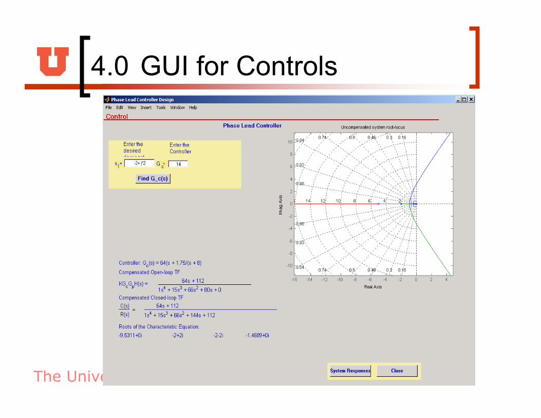
The University of Utah
4.0 GUI for Controls

The University of Utah
Concluding Remarks
� This tutorial and the GUI for Controls can be
downloaded from
� http://www.cs.utah.edu/~malko/controls/