matrix factorization methods: application to thermal ndt/e

3

Matrix factorization methods: application to Thermal NDT/E

S. Marinetti1, L. Finesso2, E. Marsilio1

1 CNR-ITC PD, C.so Stati Uniti, 4 - 35127 Padova, ITALY, ph. +39 049 829 5746, fax +39 049 829 5728 e-mail [email protected] 2 CNR-ISIB PD, C.so Stati Uniti, 4 - 35127 Padova, ITALY, ph. +39 049 829 5755, fax +39 049 829 5763 e-mail [email protected]

Abstract

A typical problem in Thermal Nondestructive Testing/Evaluation (TNDT/E) is that of unsupervised feature extraction from the experimental data. Matrix factorization methods (MFMs) are mathematical techniques well suited for this task. In this paper we present the application of three MFMs: Principal Component Analysis (PCA), Non-negative Matrix Factorization (NMF), and Archetypal Analysis (AA). To better understand the peculiarities of each method the results are first compared on simulated data. It will be shown that the shape of the data set strongly affects the performance. A good understanding of the actual shape of the thermal NDT data is required to properly choose the most suitable MFM, as it is shown in the application to experimental data.

Keywords: Thermal NDT/E, principal component analysis, non-negative matrix factorization, archetypal analysis.

1. Introduction

The basic matrix factorization problem is to represent a given matrix X∈ℜmxn as the product (X=AB) of two matrices A∈ℜmxp and B∈ℜpxn (the factors), where p is a size parameter to be properly chosen. As MFMs operate on bi-dimensional (2D) matrices and the typical output of a dynamic thermal test is generally an image sequence, that is inherently three-dimensional (3D), a pre-processing stage is needed. The thermogram sequence, representing the time evolution of a bi-dimensional temperature map, is converted into a 2D matrix X whose columns are the temporal profiles of each pixel, while rows are unrolled images. Hereafter, X will be considered as a set of temporal profiles and therefore the spatial coordinates will be neglected. The choice to privilege the temporal instead of the spatial data stems from the fact that information about the inner structure of the tested object is contained in the time evolution of the surface temperature. Given a factorization X=AB, the columns of A can be regarded as basis elements in the space of temporal profiles (i.e. as extracted features) while the rows of B are unrolled images representing reconstruction coefficients also called scores.

Factorization problems do not always have an exact solution, they are therefore often posed as approximation problems. Given X one tries to find its best approximation X≈AB by minimizing in (A,B) a chosen criterion. For a matrix M∈ℜmxm its Frobenius norm is ||M||= (∑ij=1,m mij

2)½. The approximation criterion we consider is ||X-AB||. The representational properties of the factors depend upon the constraints imposed on A, B and p.

In this paper, three approximate factorization methods, Principal Component Analysis (PCA), Non-negative Matrix Factorization (NMF), and Archetypal Analysis (AA), are applied to a typical TNDT experiment. In this context the main goals are the detection of defects and subsequently the estimation of their geometrical properties, generally based on the analysis of thermal temporal profiles. A thermal test was carried out by exciting the surface of a plastic sample with a 6 kJ energy pulse delivered in 10 ms. It is worth of mention that the use of a flash lamp as a heating source caused the surface

Keynote lecture

Proc. Vth International Workshop, Advances in Signal Processing for Non Destructive Evaluation of MaterialsQuébec City (Canada),2-4 Aug. 2005. © X. Maldague ed., É. du CAO (2006), ISBN 2-9809199-0-X

4

temperature distribution to be strongly uneven. The sample is a slab with 3 bottom holes located at depths 1.6 mm, 3.2 mm and 6.4 mm. The temperature decay of the heated surface was observed for 100 s through an infrared camera working at a sampling rate of 1 Hz. A sequence of 100 images was acquired. The sequence was then converted into a matrix X∈ℜmxn with m=100 and n=4800. Fig. 1 shows a raw thermogram 50 s after the flash (a), the mean temperature profiles of the four evidenced areas (b), and the normalized contrasts Cn (c). The performance of the three MFMs will be assessed by the degree of resemblance between the basis elements and the profiles shown in Fig. 1b and 1c.

The paper is organized in three sections containing, for each of the three MFMs, a description of the basic concepts, two case studies on simulated data for graphical interpretation, and the application to experimental data described above.

0 20 40 60 80

20

40

60

80

100

120

140

time, s

T, a

.u.

12

3 4

0 20 40 60 80 1000

0.02

0.04

0.06

0.08

0.1

0.12

time, s

Cn, a

.u.

Cn21

Cn31

Cn41

(a) (b) (c) Fig. 1: Raw thermogram (a), normalized mean temperature (in gray levels) vs. time (b), normalized

contrast vs. time (c).

2. Principal Component Analysis (PCA)

The PCA is a quite old method, originated in 1901 by Pearson [1] and later developed by Hotelling [2]. The idea behind the PCA is to fit a low dimensional hyperplane to a scatter of data points in a higher dimensional space. Data reduction is achieved projecting orthogonally the original data onto the fitted hyperplane, thus lowering the number of coordinates needed to specify their positions. This method has been recently applied in the TNDT field [3,4,5].

2.1 Basic concepts

We begin with some mathematical preliminaries. Let P≥0 be a positive semidefinite matrix in ℜmxm. It is a standard result in linear algebra that P can be represented as P = λ1u1u1

T + λ2u2u2T + … + λmumum

T

where λ1≥λ2≥ … ≥λm are the (not necessarily distinct) eigenvalues and the columns u1,…,um the corresponding eigenvectors of P (i.e. Pui= λiui). The eigenvectors can always be chosen to be an orthonormal basis of ℜm. There are two useful optimality results which are worth mentioning. For any set of orthonormal vectors w1,…,wp it is ∑i=1,pwi

TPwi ≤ ∑i=1,puiTPui = ∑i=1,p λi, and the maximum is attained

at wi=ui. For any matrix Q of rank p it is ||P-Q|| ≥ (λ2p+1 + λ2

p+2 +… + λ2m)½ and the minimum is attained at

Q = λ1u1u1T + λ2u2u2

T + … + λpupupT.

Following Pearson’s original approach, let the n columns x1,…,xn of the matrix X∈ℜmxn represent n data points in ℜm. To identify a p dimensional hyperplane in ℜm one has to specify a point contained in the hyperplane and p orthonormal axes. The best fitting hyperplane is defined as that for which the sum of the squares of the perpendiculars from the data points to the hyperplane (let us call this quantity d) is minimized. It is easy to see that the best fitting hyperplane must contain the barycentre of the data points. Without loss of generality one can therefore center the data matrix subtracting from each column of X the barycentre of the data (the average column), thus obtaining a zero column-mean matrix X’. The problem now reduces to finding the p orthogonal axes. Define the dispersion matrix as


5

P=X’X’T. If w1,…,wp are p orthonormal vectors then d=∑i=1,pPii-∑i=1,pwiTPwi. Minimizing d is equivalent to

maximizing ∑i=1,pwiTPwi which, by the first optimality result, is attained when wi=ui. Define Up∈ℜmxp as

the matrix whose i-th column is ui and Λ as the diagonal matrix with i,i-th element λi. By the orthonormality Up

TUp=Ip, the p dimensional unit matrix. By the second optimality result it follows that the minimum of ||X’X’T–Q|| among all matrices Q of rank p is attained for Q=UpΛpUp

T. The best approximate factorization of X in Frobenius norm is therefore X=AB with A=Up and B=Up

TX. Observe that p controls the approximation level, when p=m the factorization is exact.

2.2 PCA: example of application to 2D data set

Let us consider two randomly generated data sets S1 and S2. The set S1 is obtained by combining two Gaussians with different variances and rotating them by an arbitrary angle. S2 is the superposition of S1 and a similar distribution. The principal axes (Pa’s) of S1 (Fig. 2a) coincide with the main axes of the distribution. It is worth noting that the first Pa contains 94% of the total variance and therefore S1 can be considered one dimensional and well approximated by its projection onto Pa1. As for S2 (Fig. 2b), the Pa’s lack an intuitive interpretation. Moreover the eigenvalues (λ1=1.54, λ2=0.87) reveal that the information is almost evenly carried by the two Pa’s, making a one dimensional approximation unsuitable.

Pa2

Pa1

(a)

Pa2

Pa1

(b)

Fig. 2: Result of PCA applied to simulated Gaussian data.

2.3 PCA applied to experimental data

Fig. 3 shows the PCA results: the first six Pa’s (a, b), and the corresponding reconstruction coefficients (c-h). Comparing the curves in Fig. 3 with those in Fig. 1b and 1c, we note that although Pa1 and Pa3 resemble contrasts and Pa2 a temperature profile, none of the four classes can be correctly identified. Furthermore, although the images evidence the defects, they exhibit negative basis elements and reconstruction coefficients. This is the major drawback of PCA in TNDT applications as the positivity constraint is inherent in the physical data.

0 20 40 60 80-0.8-0.6-0.4-0.2

00.2

time, s

Pa,

a.u

.

Pa2

Pa3Pa1

(a)

-20

-10

0

10

20

30

40

50

Pa1 (c)

-10

-5

0

5

10

15

20

Pa2 (d)

-10

-5

0

5

10

Pa3 (e)

0 20 40 60 80

-0.2

-0.1

00.1

0.2

time, s

Pa,

a.u

.

Pa4 Pa5

Pa6

(b) -8

-6

-4

-2

0

2

4

Pa4 (f)

-2

-1

0

1

2

Pa5 (g)

-1.5

-1

-0.5

0

0.5

1

1.5

Pa6 (h)


6

Fig. 3: Principal axes (a, b) and the respective reconstruction coefficient images (c-h).

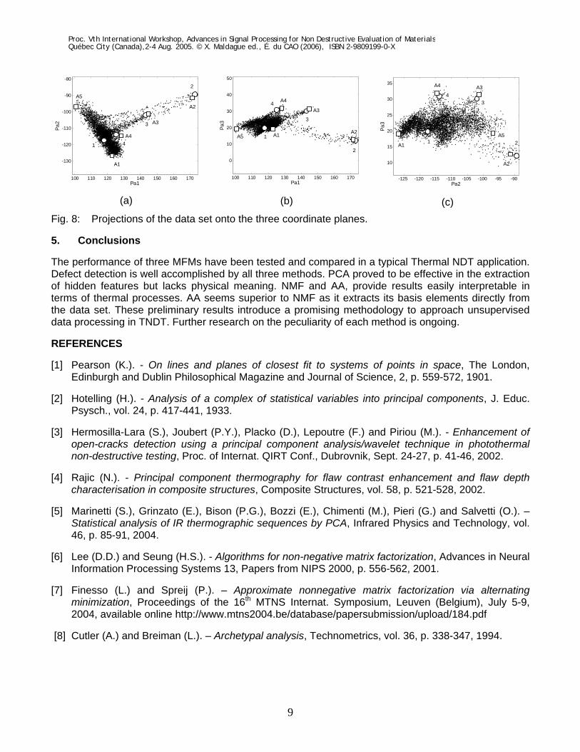
This notwithstanding, PCA is a useful tool to extract features hidden in the raw data like the stripe pattern relative to Pa6 (Fig. 3b and 3h) explained by a malfunction of the synchronization device. Another important aspect concerns the shape of the data set. The eigenvalues show that the first 3 Pa’s retain 95% of the total variance, therefore the data can be reduced by projection onto the first 3 Pa’s, thus making possible a graphical representation in ℜ3. Fig. 8 shows the orthogonal projections of the reduced data on the coordinate planes. The circles show the locations of the profiles of Fig. 1b. The sound area (circle 1) belongs to a cloud, whose dispersion is due to the uneven temperature distribution. The defect centres (circles 2-4) are located at the end of tails departing from the main cloud. The tails correspond to edge effects due to lateral heat diffusion. Their lengths and directions are likely linked to the defect depths. This representation shows that the defects are not orthogonal to each other. This accounts for the difficulty in discriminating defects assigning a specific Pa to each of them.

3. Non-negative Matrix Factorization (NMF)

NMF overcomes the interpretative difficulty of the results of PCA by imposing non-negativity constraints on both A and B, thus providing positive basis elements (generally not orthogonal to each other) and allowing only additive combinations. The NMF method was made popular by Lee and Seung [6]. The NMF is clearly applicable in the context of TNDT/E by the inherent positivity of the temperature data.

3.1 Basic concepts

Exact NMF is a long standing problem in linear algebra. Given X∈ℜ+mxn (i.e. element wise positive) and

1≤p≤min{m,n}, find a pair of matrices A∈ℜ+mxp and B∈ℜ+

pxn such that X=AB. Clearly p cannot be smaller than the rank of X, but in many cases even larger values of p do not guarantee the existence of an exact NMF. It is therefore of interest to consider the approximate NMF problem where, given X and p, one minimizes ||X-AB|| with respect to non-negative (A,B). The set of vectors Aw, where w varies freely in ℜ+

p can be interpreted geometrically as the polyhedral cone generated by the columns of A (generators of the cone). Geometrically the approximate NMF therefore consists in finding the p generators of the polyhedral cone in ℜ+

m (the p columns of A) and the n elements inside it (the n columns of AB) that best approximate the n columns of X. This optimal problem has always solution, but unlike the PCA the solution cannot be given in closed form. The main contribution of [6], is the development of an iterative algorithm which converges to local minima of ||X-AB||.

3.2 NMF: example of application to 2D data set

Let us now apply NMF to S1 and S2. Since the data sets are bi-dimensional, the exact NMF provides two vectors in the positive quadrant (N1,N2) that generate a cone containing the data points (Fig. 4). Notice that (N1,N2) is not unique, since, when the data are strictly positive (as in the case of temperature values), there are many local optima. When a cone generator is tangent to the data set, it represents a scaled version of the tangency point and therefore its physical meaning is clear. Another consideration that arises from observing Fig. 4 is the dependency of the NMF solution upon the orientation of the point cloud in the reference system.

N1

N2

N1

N2


7

(a) (b) Fig. 4: Result of NMF applied to simulated Gaussian data.

3.3 NMF applied to experimental data

NMF was applied to the experimental data with p=5. The basis elements and the score images are shown in Fig. 5. The resemblance of the basis elements to the profiles in Fig. 1b is improved with respect to PCA, however the four original classes are not separated. It is worth noting that in Fig. 5b the defects are barely visible while the uneven heating pattern appears clearly. Hence, N1 can be thought as the temperature trend common to all the pixels. Let us consider the shallowest defect, which seems the best spatially classified (Fig. 5e). In case of a correct classification, the temperature profile 2 (Fig. 1b) should be a positive linear combination of only N1 (common thermal response) and N4 (contrast signal produced by the defect). Results show that the NMF reconstruction gives significant weight also to N2 (Fig. 5c).

8.5

9

9.5

10

10.5

11

N1 (b)

3

4

5

6

7

8

9

10

N2 (c)

0.05

0.1

0.15

0.2

0.25

0.3

0.35

N3 (d)

0 20 40 60 800

2

4

6

8

10

12

time, s

NM

F co

mpo

nent

, a.u

.

N1

N2

N3N4

N5

(a)

0

1

2

3

4

5

N4 (e)

0

0.2

0.4

0.6

0.8

1

1.2

N5 (f)

Fig. 5: Non-negative components (a) and the respective reconstruction coefficient images (b-f).

4. Archetypal Analysis (AA)

The AA, proposed by Cutler and Breiman in 1994 [8], approximates each point in the set (individual) as a convex combination of basis elements called archetypes. The archetypes are themselves convex combinations of the individuals in the data set. In the application to the TNDT/E field, the archetypes are pure temporal profiles. Depending on the shape of the data set, the archetypal profiles may correspond to some individuals thus affording an easier interpretation of their physical meaning.

4.1 Basic concepts

In archetypal analysis one uses as basis elements convex combinations of the columns of X. We remind the reader that the convex hull of two vectors is the segment joining them while given n vectors their convex hull is the smallest convex set containing all of them. Given a matrix X∈ℜmxn, the convex hull of its columns xi is the set of vectors w= Σi=1,nγixi where the γi≥0 vary under the constraint Σi=1,nγi=1. A matrix C∈ℜnxp is called column stochastic if it has columns with positive elements adding to 1. By the previous definitions it follows that if C is column stochastic the columns of XC are contained in the convex hull of the columns of X. The AA factorization problem can now be stated as follows: assigned a matrix X∈ℜmxn and an integer p find, in the convex hull of the columns of X, a set of p vectors (the columns of XC for a proper stochastic matrix C) whose convex combinations can optimally represent X in the Frobenius norm, i.e. minimize ||X - XCB||. The solution to the approximate AA factorization is therefore given by the pair (A,B)=(XC,B) of respective sizes nxp and pxm. The solution is computed by


8

solving a non linear least squares problem with convexity constraints. The relation between AA and NMF is shortly discussed in [7].

4.2 AA: example of application to 2D data set

Results provided by AA applied to S1 (p=2) and S2 (p=3) are reported in Fig. 6. The main difference with respect to PCA and NMF is that the archetypes do not represent directions, rather they are points on the boundary of the convex hull of the data set. This allows a more straightforward interpretation of their physical meaning. As for the data reconstruction, all the points of S1 are projected onto the segment A1-A2 (Fig. 6a), the points of S2 (Fig. 6b) that are inside the triangle are exactly reconstructed while those laying outside are projected onto the closest edge.

A2

A1

(a)

A1

A3A2

(b)

Fig. 6: Result of AA applied to simulated Gaussian data.

4.3 Applications to experimental data

AA, like NMF, requires the preliminary choice of the number p of archetypes. Once again we chose p=5. Indeed, looking at Fig. 8, that represents a good view of the experimental data set, it seems plausible to expect that three archetypes could fall on the three defects 2,3 and 4, the other two archetypes should fall onto the extreme points of the cloud corresponding to the sound material.

0

0.2

0.4

0.6

0.8

1

A1 (b)

0

0.2

0.4

0.6

0.8

1

A2 (c)

0

0.2

0.4

0.6

0.8

1

A3 (d)

0 20 40 60 80

20

40

60

80

100

120

140

A1

A2A3 A4

A5

(a)

0

0.2

0.4

0.6

0.8

A4 (e)

0

0.2

0.4

0.6

0.8

1

A5 (f)

Fig. 7: Archetypes (a) and the respective reconstruction coefficient images (b-f).

Results shown in Fig. 7 confirmed the expectations. Indeed, defects 2 and 3 are represented just by one archetype each (A2 and A3 respectively), 90% of defect 4 is described by A4 and the remaining 10% by A1 and A5, that are the archetypes associated to the sound area. Fig. 8 is a graphic representation of the archetype locations where the dots are the data points, the circles the raw profiles 1-4 (Fig. 1b) and the squares the archetypes A1-A5.


9

100 110 120 130 140 150 160 170

-130

-120

-110

-100

-90

-80

Pa1

Pa2

1

2

3

4

A1

A2

A3

A4

A5

(a)

100 110 120 130 140 150 160 170

0

10

20

30

40

50

Pa1

Pa3

1

2

3

4

A1 A2

A3

A4

A5

(b)

-125 -120 -115 -110 -105 -100 -95 -90

10

15

20

25

30

35

Pa2

Pa3

1 2

34

A1

A2

A3A4

A5

(c) Fig. 8: Projections of the data set onto the three coordinate planes.

5. Conclusions

The performance of three MFMs have been tested and compared in a typical Thermal NDT application. Defect detection is well accomplished by all three methods. PCA proved to be effective in the extraction of hidden features but lacks physical meaning. NMF and AA, provide results easily interpretable in terms of thermal processes. AA seems superior to NMF as it extracts its basis elements directly from the data set. These preliminary results introduce a promising methodology to approach unsupervised data processing in TNDT. Further research on the peculiarity of each method is ongoing.

REFERENCES

[1] Pearson (K.). - On lines and planes of closest fit to systems of points in space, The London, Edinburgh and Dublin Philosophical Magazine and Journal of Science, 2, p. 559-572, 1901.

[2] Hotelling (H.). - Analysis of a complex of statistical variables into principal components, J. Educ. Psysch., vol. 24, p. 417-441, 1933.

[3] Hermosilla-Lara (S.), Joubert (P.Y.), Placko (D.), Lepoutre (F.) and Piriou (M.). - Enhancement of open-cracks detection using a principal component analysis/wavelet technique in photothermal non-destructive testing, Proc. of Internat. QIRT Conf., Dubrovnik, Sept. 24-27, p. 41-46, 2002.

[4] Rajic (N.). - Principal component thermography for flaw contrast enhancement and flaw depth characterisation in composite structures, Composite Structures, vol. 58, p. 521-528, 2002.

[5] Marinetti (S.), Grinzato (E.), Bison (P.G.), Bozzi (E.), Chimenti (M.), Pieri (G.) and Salvetti (O.). – Statistical analysis of IR thermographic sequences by PCA, Infrared Physics and Technology, vol. 46, p. 85-91, 2004.

[6] Lee (D.D.) and Seung (H.S.). - Algorithms for non-negative matrix factorization, Advances in Neural Information Processing Systems 13, Papers from NIPS 2000, p. 556-562, 2001.

[7] Finesso (L.) and Spreij (P.). – Approximate nonnegative matrix factorization via alternating minimization, Proceedings of the 16th MTNS Internat. Symposium, Leuven (Belgium), July 5-9, 2004, available online http://www.mtns2004.be/database/papersubmission/upload/184.pdf

[8] Cutler (A.) and Breiman (L.). – Archetypal analysis, Technometrics, vol. 36, p. 338-347, 1994.


matrix factorization methods: application to thermal ndt/e

Documents