matroid polytope subdivisions and...
TRANSCRIPT

Matroid polytope subdivisions and valuations
by
Alexander Ray Fink
A dissertation submitted in partial satisfaction of the
requirements for the degree of
Doctor of Philosophy
in
Mathematics
in the
Graduate Division
of the
University of California, BERKELEY
Committee in charge:
Professor Bernd Sturmfels, ChairProfessor Federico ArdilaProfessor David EisenbudProfessor Robion KirbyProfessor Satish Rao
Spring 2010

Matroid polytope subdivisions and valuations
Copyright 2010
by
Alexander Ray Fink
1
Abstract
Matroid polytope subdivisions and valuations
by
Alexander Ray Fink
Doctor of Philosophy in Mathematics
University of California, BERKELEY
Professor Bernd Sturmfels, Chair
Many important invariants for matroids and polymatroids are valuations (or are valuative),which is to say they satisfy certain relations imposed by subdivisions of matroid polytopes.These include the Tutte polynomial, the Billera-Jia-Reiner quasi-symmetric function, Derk-sen’s invariant G, and (up to change of variables) Speyer’s invariant h.
We prove that the ranks of the subsets and the activities of the bases of a matroid definevaluations for the subdivisions of a matroid polytope into smaller matroid polytopes; thisprovides a more elementary proof that the Tutte polynomial is a valuation than previouslyknown.
We proceed to construct the Z-modules of all Z-valued valuative functions for labeledmatroids and polymatroids on a fixed ground set, and their unlabeled counterparts, the Z-modules of valuative invariants. We give explicit bases for these modules and for their dualmodules generated by indicator functions of polytopes, and explicit formulas for their ranks.This confirms Derksen’s conjecture that G has a universal property for valuative invariants.
We prove also that the Tutte polynomial can be obtained by a construction involvingequivariant K-theory of the Grassmannian, and that a very slight variant of this constructionyields Speyer’s invariant h. We also extend results of Speyer concerning the behavior ofsuch classes under direct sum, series and parallel connection and two-sum; these resultswere previously only established for realizable matroids, and their earlier proofs were moredifficult.
We conclude with an investigation of a generalisation of matroid polytope subdivisionsfrom the standpoint of tropical geometry, namely subdivisions of Chow polytopes. The Chowpolytope of an algebraic cycle in a torus depends only on its tropicalisation. Generalis-ing this, we associate a Chow polytope subdivision to any abstract tropical variety in Rn.Several significant polyhedra associated to tropical varieties are special cases of our Chowsubdivision. The Chow subdivision of a tropical variety X is given by a simple combinatorial

2
construction: its normal subdivision is the Minkowski sum of X and an upside-down tropicallinear space.

i
Contents
1 Overview 1
1.1 Matroids and their polytopes . . . . . . . . . . . . . . . . . . . . . . . . . . 1
1.2 Subdivisions and valuations . . . . . . . . . . . . . . . . . . . . . . . . . . . 3
1.3 Matroids and the Grassmannian . . . . . . . . . . . . . . . . . . . . . . . . . 7
1.4 Tropical geometry . . . . . . . . . . . . . . . . . . . . . . . . . . . . . . . . . 10
2 Valuations for matroid polytope subdivisions 13
2.1 Introduction . . . . . . . . . . . . . . . . . . . . . . . . . . . . . . . . . . . . 13
2.2 Preliminaries on matroids and matroid subdivisions . . . . . . . . . . . . . . 14
2.3 Valuations under matroid subdivisions . . . . . . . . . . . . . . . . . . . . . 17
2.4 A powerful family of valuations . . . . . . . . . . . . . . . . . . . . . . . . . 20
2.5 Subset ranks and basis activities are valuations . . . . . . . . . . . . . . . . 23
2.5.1 Rank functions . . . . . . . . . . . . . . . . . . . . . . . . . . . . . . 23
2.5.2 Basis activities . . . . . . . . . . . . . . . . . . . . . . . . . . . . . . 24
2.6 Related work . . . . . . . . . . . . . . . . . . . . . . . . . . . . . . . . . . . 29
3 Valuative invariants for polymatroids 32
3.1 Introduction . . . . . . . . . . . . . . . . . . . . . . . . . . . . . . . . . . . . 32
3.2 Polymatroids and their polytopes . . . . . . . . . . . . . . . . . . . . . . . . 37
3.3 The valuative property . . . . . . . . . . . . . . . . . . . . . . . . . . . . . . 42
3.4 Decompositions into cones . . . . . . . . . . . . . . . . . . . . . . . . . . . . 46
3.5 Valuative functions: the groups PM, PPM, PMM . . . . . . . . . . . . . . . . . 49
3.6 Valuative invariants: the groups P symM , P sym
PM , P symMM . . . . . . . . . . . . . . . 55
3.7 Hopf algebra structures . . . . . . . . . . . . . . . . . . . . . . . . . . . . . . 61
3.8 Additive functions: the groups TM, TPM, TMM . . . . . . . . . . . . . . . . . . 65
3.9 Additive invariants: the groups T symM , T sym
PM , T symMM . . . . . . . . . . . . . . . . 73

ii
3.10 Invariants as elements in free algebras . . . . . . . . . . . . . . . . . . . . . . 74
3.A Equivalence of the weak and strong valuative properties . . . . . . . . . . . . 77
3.B Tables . . . . . . . . . . . . . . . . . . . . . . . . . . . . . . . . . . . . . . . 82
3.C Index of notations used in this chapter . . . . . . . . . . . . . . . . . . . . . 84
4 The geometry of the Tutte polynomial 86
4.1 Introduction . . . . . . . . . . . . . . . . . . . . . . . . . . . . . . . . . . . . 86
4.1.1 Notation . . . . . . . . . . . . . . . . . . . . . . . . . . . . . . . . . . 88
4.2 Background on K-theory . . . . . . . . . . . . . . . . . . . . . . . . . . . . . 89
4.2.1 Localization . . . . . . . . . . . . . . . . . . . . . . . . . . . . . . . . 91
4.3 Matroids and Grassmannians . . . . . . . . . . . . . . . . . . . . . . . . . . 94
4.4 Valuations . . . . . . . . . . . . . . . . . . . . . . . . . . . . . . . . . . . . . 98
4.5 A fundamental computation . . . . . . . . . . . . . . . . . . . . . . . . . . . 100
4.6 Flipping cones . . . . . . . . . . . . . . . . . . . . . . . . . . . . . . . . . . . 102
4.7 Proof of the formula for the Tutte polynomial . . . . . . . . . . . . . . . . . 106
4.8 Proof of the formula for Speyer’s h . . . . . . . . . . . . . . . . . . . . . . . 109
4.9 Geometric interpretations of matroid operations . . . . . . . . . . . . . . . . 112
5 Tropical cycles and Chow polytopes 118
5.1 Introduction . . . . . . . . . . . . . . . . . . . . . . . . . . . . . . . . . . . . 118
5.2 Setup . . . . . . . . . . . . . . . . . . . . . . . . . . . . . . . . . . . . . . . . 119
5.2.0 Polyhedral notations and conventions . . . . . . . . . . . . . . . . . . 119
5.2.1 Tropical cycles . . . . . . . . . . . . . . . . . . . . . . . . . . . . . . 119
5.2.2 Normal complexes . . . . . . . . . . . . . . . . . . . . . . . . . . . . 122
5.2.3 Chow polytopes . . . . . . . . . . . . . . . . . . . . . . . . . . . . . . 123
5.3 Minkowski sums of cycles . . . . . . . . . . . . . . . . . . . . . . . . . . . . . 128
5.4 From tropical variety to Chow polytope . . . . . . . . . . . . . . . . . . . . . 130
5.5 Linear spaces . . . . . . . . . . . . . . . . . . . . . . . . . . . . . . . . . . . 133
5.6 The kernel of the Chow map . . . . . . . . . . . . . . . . . . . . . . . . . . . 137
Bibliography 140

iii
Acknowledgements
I have benefitted from talking to a great number of mathematicians in the course of thiswork, and to them my sincere thanks are due. Among them are my coauthors, FedericoArdila and Edgard Felipe Rincon, Harm Derksen, and David Speyer; I also thank BerndSturmfels, Allen Knutson, Megumi Harada, Sam Payne, Johannes Rau, and Eric Katz, andmany others I haven’t named. Multiple anonymous referees have made useful suggestions aswell: one made suggestions leading to Table 2.2 and Proposition 2.6.1. I also thank BerndSturmfels and Federico Ardila for their guidance and oversight of during the course of thiswork and their suggestions of interesting problems.
The work of Chapter 2 was carried out as part of the SFSU-Colombia CombinatoricsInitiative. I am grateful to the San Francisco State University for their financial support ofthis initiative, and to the Universidad de Los Andes for supporting Rincon’s visit to SFSUin the Summer of 2007. Work with Speyer led to a proof of Theorem 3.1.4 before my maincollaboration with Derksen described in Chapter 3. Chapter 4 was finished while Speyer andI visited the American Institute of Mathematics, and we are grateful to that institution forthe many helpful conversations they fostered.

1
Chapter 1
Overview
1.1 Matroids and their polytopes
The matroid is a combinatorial structure with many faces. Not only is it widely applicablein mathematics, it can be formalised in a large number of ways which, on the surface, don’tlook equivalent. Basically, a matroid abstracts the properties of an independence relation ofwhatever nature on a finite set. Let E be a finite set, of cardinality n. We will often takeE = [n] := 1, 2, . . . , n, which is a completely general choice: we only care about E up tobijections of sets. For simplicity we give only one definition of a matroid M on the groundset E, that in terms of bases. We say that a set B of subsets of E is the set of bases B(M) ofa matroid M if it satisfies the following axioms:
• B 6= 0;
• For any B,B′ ⊆ B and b′ ∈ B′ \ b, there exists b ∈ B \B′ such that B ∩ b \ b′ ∈ B(the exchange axiom).
The axioms could also be cast to capture other data associated to M , such as the inde-pendent sets I(M), the set of all subsets of E contained in a basis, or the rank function rkM
on subsets A ⊆ E such that rkM(A) is the size of the largest intersection of A with a basis.
For instance, the first and paramount example of an independence relation is linearindependence of vectors in a vector space. Let E = v1, . . . , vn be a subset of a vectorspace V . Then there is a matroid M on E whose bases B(M(V )) are the subsets of E formingvector space bases for span E, whose independent sets I(M) are the linearly independentsubsets of E, and whose rank function is rkM(A) = dim spanA. We say that a matroidis representable over a given field K if and only if it has this form for some V a K-vectorspace. Representable matroids are a class of fundamental importance to matroid theory —but equally one could say that it’s the frequency with which combinatorial situations with

2
underlying vector arrangements extend to non-representable matroids that makes matroidtheory shine. We’ll see two examples of this in later sections.
We will be particularly concerned here with certain functions on matroids. Before de-veloping the conditions characterising these, we discuss an example of such a function: theTutte polynomial, probably the best-known function on matroids. The Tutte polynomialis an invariant: it takes equal values on isomorphic matroids. We’ll talk about it at somelength, both on account of its own importance (several of our results concern it) and becauseits story parallels one of our main themes.
The Tutte polynomial t(M) of a matroid M is a bivariate polynomial,
t(M) =∑A⊆E
(x− 1)rkM (E)−rkM (A)(y − 1)|A|−rkM (A) .
This presentation is known as the rank generating function; the two quantities in the exponentcan be taken as measuring how far off A is from a basis in two different senses, given that|B| = rk(B) = rk(E) when B is a basis. There is another presentation in terms of internaland external activities; we defer to Section 2.5 for the statement.
Example 1.1.1. The bases of the rank r uniform matroid UE,r on E are all subsets of E ofsize r. Its Tutte polynomial is
t(UE,r) = (x− 1)r +
(n
1
)(x− 1)r−1 + · · ·+
(n
r − 1
)(x− 1)
+
(n
r
)+
(n
r + 1
)(y − 1) + · · ·+
(n
n− 1
)(y − 1)n−r−1 + (y − 1)n−r. ♦
Tutte took interest in the fact that the number of spanning trees of a graph could becomputed recursively in terms of certain graph minors. In fact the set of spanning treesof a graph G are the bases of a matroid on the ground set Edges(G). In this light thestatement becomes the more transparent one that the number of bases of M satisfies thedeletion-contraction recurrence,
f(M) =
f(M \ e) + f(M/e) e not a loop or coloop,f(M \ e)f(e) e a loop,f(M/e)f(e) e a coloop.
(1.1.1)
A loop in M is an element e ∈ E contained in no basis; a coloop is one contained in everybasis. M \ e is the matroid on E \ e whose bases are the bases of M not containing e; M/eis the matroid on the same set E \ e whose bases are the bases of M containing e, with eremoved.
Several other invariants f : matroids → R of interest, for a ring R, also satisfy thedeletion-contraction recurrence, among them other basic properties like number of indepen-dent sets, and invariants with nontrivial graph-theoretic content like the chromatic poly-nomial. Tutte defined the Tutte polynomial and showed that it had a universal property

3
([88] but there only for graphs; Crapo in [23] does the general case), solving the problem ofclassifying all invariants satisfying the deletion-contraction recurrence.
Theorem 1.1.2. Let f be a matroid invariant satisfying (1.1.1). Then f = f ′ t for somering homomorphism f ′. Explicitly, f(M) = t(M)(f(coloop), f(loop)).
(By ‘coloop’ and ‘loop’ here we refer to matroids on a singleton ground set whose onlyelement is a coloop, respectively a loop.)
The main perspective on matroids adopted by this thesis takes them as polytopes. (Apolyhedron is an intersection of half-spaces; a polytope is a bounded polyhedron, equivalentlythe convex hull of finitely many points. A lattice polytope or polyhedron is one whose verticesare contained in a fixed lattices.)
Fix a real vector space RE with a distinguished basis ei : i ∈ E and its dual basisei : i ∈ E. For a set I ⊆ E, we write eI =
∑i∈I ei for the zero-one indicator vector of I.
Given a matroid M on E, its matroid polytope is
Poly(M) = conveB : B ∈ B(M).
The next theorem gives a pleasant intrinsic characterisation of matroid polytopes, which canbe taken as another axiom system for matroids.
Theorem 1.1.3 (Gelfand-Goresky-MacPherson-Serganova [37]). A polytope Q ⊆ RE is amatroid polytope if and only if
• every vertex of Q is of the form eI for I ⊆ E, and
• every edge of Q is of the form eI∪i, eI∪j for i, j 6∈ I ⊆ E.
The second of these conditions of course implies the first, unless Q is a point.
Matroid polytopes were first studied in connection with optimisation and with the ma-chinery of linear programming, introduced there by Edmonds [33] (who in fact treated amild variant of Poly(M), defined as the convex hull of all independent sets). A second lineof inquiry regarding matroid polytopes springs from the observation that their edge vectorsare the roots of the An root system. Generalisations to other root systems are then studied:these are the Coxeter matroids [14]. Most recently, matroid polytopes have appeared in anumber of related algebraic-geometric contexts. We go into this in more detail in Section 1.3.
1.2 Subdivisions and valuations
The central construction in which matroid polytopes are involved in this thesis are sub-divisions. Let P be a set of closed convex sets in a real vector space V ; in our case P is the

4
set of matroid polytopes, together with the empty set. A subdivision of sets in P is a cellcomplex Σ in V whose underlying space Σ is in P and such that, if P1, . . . , Pk are the maxi-mal cells of V , every intersection PK :=
⋂k∈K Pk (∅ 6= K ⊆ [k]) of some of these cells is in P .
For uniformity we put P∅ = |Σ|. Since faces of a matroid polytope are matroid polytopesby Theorem 1.1.3, Σ is a matroid polytope subdivision as soon as |Σ| and the maximal cellsPi are matroid polytopes. For example, Figure 1.1 portrays the simplest nontrivial matroidpolytope subdivision.
10011010
1010
1010
0011
1100
01101001
0110
0101
1001 01010110
0101
Figure 1.1: The matroid subdivision of a regular octahedron into two square pyramids.
Let G be an abelian group. A function f : P → G is a valuation if, for any subdivisionΣ of sets in P with the PK defined as above, we have∑
K⊆[k]
(−1)|K|f(PK) = 0. (1.2.1)
That is, valuations are functions that add in subdivisions, taking account of the overlaps atthe boundaries of the maximal cells. We require that valuations take value 0 on ∅.
Valuations are a topic of classical interest; their defining property is similar to that ofmeasures, and they’re a basic tool in convexity. Among their uses is that they help us gaincontrol over the possible structures of subdivisions, and thus over the structures subdivisionscharacterise. For instance, if an integer-valued function f is positive and is zero on polytopesnot of full dimension, then any full-dimensional polytope P can be subdivided into at mostf(P ) pieces in P . (This is essentially the situation with Speyer’s invariant h introduced atthe end of Section 1.3.)
One fundamental valuation is the indicator function: indeed, the way (1.2.1) accountsfor overlaps is exactly what’s needed for the indicator function to be valuative. As usual, the

5
indicator function of a set P ⊆ RE is the map of sets 1(P ) : RE → Z for which 1(P )(x) = 1if x ∈ P and 1(P )(x) = 0 otherwise; by the unadorned name “the indicator function”,referring to a function on P , we mean 1 : P → HomSet(RE,Z).
Just as for the deletion-contraction recurrence (1.1.1), it turns out that several interestingfunctions of matroids are valuations on matroid polytopes. The Tutte polynomial is one.Some others have been recently introduced by Derksen [29], Billera, Jia and Reiner [11], andSpeyer [83]. In addition there is interest in certain properties of matroid polytopes whichare self-evidently valuations, such as their volume [5] or their Ehrhart polynomial [30], butwhich are otherwise little understood.
If all sets in P are bounded, another basic valuation is the function χ taking the value 1on every nonempty set in P . This can be thought of as the Euler characteristic, and fromthis perspective checking that χ is a valuation essentially amounts to repeated applicationof the Mayer-Vietoris sequence. Chapter 2 is an investigation of valuations that can beconstructed from χ. The flexibility in this situation is this: if X is a closed convex set, andΣ is a subdivision, then Σ∩X with the cell structure given by intersecting cells of Σ with Xis a subdivision too. So M 7→ χ(Poly(M) ∩X) is a valuation. These are a generalisation ofevaluations of 1 (take X to be a point).
In Chapter 2, after setting this machinery up, we use it to build some families of valuationswhich encapsulate a lot of information about matroids. The first family is the characteristicfunctions of ranks of sets, or more generally of chains of sets.
Theorem 2.5.1, Proposition 2.6.1. The function
sA,r(M) =
1 rkM(Ai) = ri for all i0 otherwise
(1.2.2)
is a matroid valuation, for any chain ∅ A1 ⊆ · · · ⊆ Ak ⊆ E and r = (r1, . . . , rk) ∈ Zk.
The second family is the characteristic function of internal and external activities ofbases.
Theorem 2.5.4. The function
fB,I,E(M) =
1 B ∈ B(M) has internal activity I and external activity E0 otherwise
is a matroid valuation, for any subsets B, I, E ⊆ E.
One can construct the Tutte polynomial T as a linear combination of either of thesefamilies, yielding more elementary proofs that T is valuative than previously known (Corol-lary 2.5.7).
We return to the question of characterising all valuations. Chapter 3 is dedicated tothis question in a range of settings. One generalisation we make throughout that chapter

6
is to polymatroids, another structure of general interest introduced by Edmonds. We alsoinvoke megamatroids, which are primarily a technical tool. The polytopes of polymatroidsare characterised by a close variant of Theorem 1.1.3: they are those lattice polytopes in thepositive orthant whose edges are parallel to vectors of the form ei−ej but have no restrictionson length. Rank functions can also be defined for polymatroids. Finally, megamatroidpolyhedra are simply the unbounded analogues of polymatroid polytopes.
If f is a valuation, then so is g f for any group homomorphism g. Thus one could askfor a universal valuation which all valuative functions of matroids factor through, parallelto Theorem 1.1.2. One natural candidate for a universal valuation is 1. (In the languagewith which Chapter 3 begins, valuations which factor through 1 are strong valuations, andfunctions satisfying (1.2.1) are weak valuations.) This works in several classical cases: everyvaluation does factor through 1 when P is the set of all convex bodies [41], and when P isa set of convex bodies closed under intersection [91]. But these do not subsume the case ofmatroid polytopes.
Example 1.2.1. Half a regular octahedron as in Figure 1.1 is a matroid polytope, as is anyof its images under the S4 symmetries of the octahedron, where S denotes the symmetricgroup. But a quarter octahedron can be obtained as the intersection of two of these images,and this is not a matroid polytope. ♦
The first substantive result of Chapter 3 establishes that 1 is indeed a universal valuationfor matroids and polymatroids.
Theorem 3.3.5. Any valuation f of matroids or polymatroids is of the form f ′ 1 for somegroup homomorphism f ′.
Valuativity is a linear condition (unlike (1.1.1)), and so the set of valuative functions on(poly)matroids on [n] of rank D, valued in a ring R, is an R-module. A few conditions on Rbecome necessary; everything will work as stated if R = Q. To keep the notation light, wecall the module of valuations V (n, r) for the moment, and ignore notationally the question ofwhether it’s matroids or polymatroids we’re dealing with. (In the more fastidious notationof Chapter 3, we use the symbol P(P)M(n, r)∨.) By definition, V (n, r) is dual to the quotientof the free module on the set of (poly)matroids by relations like (1.2.1). Theorem 3.3.5 abovegives us a set of generators of V (n, r), namely the indicator functions of points. For greatercontrol we might ask for a presentation in generators and relations. In fact, in the cases wecare about, V (n, r) will be a free module and we can find a basis. This is the aim of the restof Chapter 3.
It turns out that the sA,r from (1.2.2) generate V (n, r) for matroids and polymatroids,and it’s easy to get a basis with a little care paid to the index set.
Corollary 3.5.5. A basis for V (n, r) consists of those sA,r such that sA,r is not identicallyzero and is not equal to any sA′,r′ for A′, r′ subsequences of A, r (i.e. none of the equationsrkM(Ai) = ri are redundant).

7
A near-exact analogue is true for the module of valuative invariants, which could bewritten V (n, r)Sn : we could modify Corollary 3.5.5 by imposing only the condition that Ais a subsequence of a fixed maximal chain of sets. But in this case the statement is nicer ina variant:
Corollary 3.6.4. A basis for V (n, r)Sn consists of those sA,r such that sA,r is not identicallyzero and A is the chain [1] ⊆ [2] ⊆ · · · ⊆ [n].
The chapter culminates in a very clean algebraic description of the modules of valuativeinvariants on all (poly)matroids, where now n and r are allowed to vary, and we considerV S∞ , the direct sum of the V (n, r)Sn over all n and r. There is also a clean structure foradditive valuations, those valuations whose values are zero on matroid polytopes of non-maximal dimension.
Theorem 3.1.7. The module V S∞ is a free associative algebra over R, in the generatorsspt,r. The submodule of additive valuations is the free Lie algebra on these generators,included in V S∞ by [a, b] 7→ ab− ba.
The multiplication invoked here is essentially such that the sA,r multiply by catenatingsubscripts. This is, moreover, the natural product structure that is associated with valuationsin the Hopf algebra structures on (poly)matroids and their valuations which we introduce insection 3.7. (Poly)matroids thus have a place in the study of combinatorial Hopf algebras,a recent active area of research [1].
1.3 Matroids and the Grassmannian
Let K be an algebraically closed field of characteristic 0.1 The Grassmannian Gr(d,E) isthe space parametrising d-dimensional vector subspaces of KE. It is a projective variety: itembeds into the projectivisation of
∧dKE by the Plucker embedding, which sends a subspaceV to the wedge product of a basis of V . The Plucker coordinates are the correspondingprojective coordinates. There are
(nd
)Plucker coordinates pi1···id , one for each basis element
ei1 ∧ · · · ∧ eid of∧dKE. (Recall that n = |E|.)
By the Gelfand-MacPherson correspondence, the Grassmannian is the parameter spacefor a second kind of object, namely arrangements of n vectors in Kd modulo the GLd action.The correspondence has an elementary description: given an d× n matrix A over K whoserowspan is a d-dimensional subspace V ⊆ Kn, the corresponding vector arrangement consistsof the columns of A. So, given a point x ∈ Gr(d,E), consider its support B in the Pluckercoordinates. Using the hyperplane arrangement description, we see that this B is the set ofbases of a representable matroid M(x).
1In other words we may as well choose K = C.

8
Here is a more geometric setting in which M(x) is encountered. Consider the n-dimensional algebraic torus T := (K∗)E. There is a natural action of T on Gr(d,E), bywhich the ith coordinate of T scales the ith vector in the arrangement (observe that thisscaling does not change M(x)). The same action can be defined by letting T act on KE
coordinatewise and carrying out the constructions in the first paragraph equivariantly; inparticular this action is a restriction from a T -action on P(
∧dKE). If x is a point of a(projectivised) K-vector space with a T -action, there is an associated weight polytope, givenas the convex hull of the characters T acts by on the smallest T -invariant vector subspacecontaining x. In the case at hand. the weight polytope of x ∈ Gr(d,E) is Poly(M(x)). Arelated way to say this: given x, the variety Tx, the closure of the orbit of x under theT -action is a toric variety. Toric varieties are a very tractable class of algebraic varieties,due in no small part to their combinatorial nature. In particular, to every lattice polytopeis associated a toric variety, and in our case, Tx is the variety associated to the polytopePoly(M(x)).
Matroid subdivisions have made prominent appearances in algebraic geometry, such as incompactifying the moduli space of hyperplane arrangements (Hacking, Keel and Tevelev [42]and Kapranov [46]), compactifying fine Schubert cells in the Grassmannian (Lafforgue [55,56]), as well as Speyer’s h below. Lafforgue’s work implies, for instance, that a matroidwhose polytope has no subdivisions is representable in at most finitely many ways, up to theactions of the obvious groups.
Underlying these appearances are certain degenerations which can be constructed over afield with a valuation ν. (We have here an unfortunate collision of terminology: a valuationon a field, i.e. a homomorphism from its group of units to an ordered group, has nothingto do with a valuation of polytopes.) Our variety Tx ⊆ Gr(d,E) degenerates into reduciblevarieties Y1 ∪ · · · ∪Yk such that each nonempty intersection
⋂i∈I Yi of components is again a
torus orbit closure of form TyI . Associated to this degeneration is a subdivision of the weightpolytope of Tx into the weight polytopes of the various TyI , with identical combinatorics:i.e. the facets are the Poly(M(yi)), and we have
⋂i∈I Poly(M(yi)) = Poly(M(yI)). The
subdivision is constructed by lifting the vertices of the weight polytope into one more di-mension, in a fashion encoding certain values of ν. The faces of the lifted polytope which arevisible from the direction of lifting form the subdivision in question. This is what’s knownas a regular subdivision. Figure 1.2 is an example of a regular subdivision.
Starting with a representable matroid M(x), we have constructed a subvariety Tx ofGr(d,E). This opens a set of avenues for the study of matroids by geometric means, throughworking with the classes of the Tx in cohomology theories of Gr(d,E) (for instance the Chowcohomology). Given our concern with valuations, the natural cohomology theory to useis algebraic K-theory : more precisely we only need the 0th K-theory functor K0. This isdefined in Section 4.2. For the present purposes we need only a few facts. When X is asufficiently nice variety, like all those we will be working with, K0(X) is a ring. To everysubvariety Y ⊆ X corresponds an element [Y ] ∈ K0(X). The key property is this: when a

9
2 1 1 0 1
Figure 1.2: The regular subdivision of a 1-dimensional polytope with specified lifting heights.
variety Y = Y1 ∪ Y2 is reducible, the relation
[Y ]− [Y1]− [Y2] + [Y1 ∪ Y2] = 0
holds in K0[X]. Note the analogy with (1.2.1). We have similar relations for reduciblevarieties Y ⊆ X with any number of components. The degeneration of Tx we describe in thelast paragraph doesn’t affect K-theory class. Altogether, this shows that the map M(x) 7→y(M(x)) := [Tx] ∈ K0(Gr(d,E)) is a valuation of representable matroids. Multiplicationbeing a linear map, the same is true of M(x) 7→ Cy(M(x)) for any class C ∈ K0(Gr(d,E)).
Actually, we mostly use a richer functor, the equivariant K-theory K0T (X), which retains
some information about the way the torus T acts on all the varieties in question. Theproperties above also hold of K0
T (X). Our main technical tool in Chapter 4 is equivariantlocalisation. This reduces computations in the ring K0(Gr(d,E)) to computations in a directsum of copies of K0
T (point) = Z[t±11 , . . . , t±1
n ], the ring of Laurent polynomials in n variables(or, canonically, the group ring of the characters of T ); there is no parallel to this reductionin the non-equivariant case. This is of great computational utility. The computations ofequivariant localisation have a very strong polyhedral flavour, and our proofs end up mainlydealing in lattice point generating functions of the matroid polytope and related polyhedra.
We would of course like to be able to work with all matroids, not just the representableones M(x) which we started with above. It is a remarkable fact, proved in [83], that eventhough nonrepresentable matroids M have no corresponding subvarieties they still haveassociated classes y(M) in K0
T (Gr(d,E)), which can be computed from their polytopes. Wecan treat valuations on the set of all matroids this way.
Following the track of the previous chapters, we might ask whether the valuations ofthe form M(x) 7→ C[Tx] generate all valuations. It turns out they don’t (Example 4.4.4).However, we can construct two important valuations in terms of these, and these are the

10
main results of Chapter 4. The first is the Tutte polynomial. The second is Speyer’s invarianth which is the subject of [83]. Speyer conjectures (and has proven in several cases) that, upto a change of variable, h is positive; if this were true, it would impose sharp upper boundson the number of faces possible of each dimension in a matroid polytope subdivision.
Though we won’t define all the necessary objects in this exposition, we state the maintheorems here to highlight the striking formal similarity between the two invariants.
Theorems 4.7.1, 4.8.5. There exist maps and varieties Gr(d,E)π← F`
π′→ (Pn−1 × Pn−1)such that
t(M)(α, β) = (π′)∗π∗(y(M) · [O(1)])
h(M)(α, β) = (π′)∗π∗(y(M))
where (π′)∗ and π∗ are respectively pushforward and pullback in K-theory, and K0(Pn−1 ×Pn−1) = Z[α, β]/(αn, βn).
1.4 Tropical geometry
Our last chapter, Chapter 5, lies outside the thread of the other chapters regardingmatroid valuations. Instead it builds off the appearances of matroids in tropical geometry,and consists of some first steps towards a generalisation.
Tropical geometry is a relatively new field of study. At its beginnings lies the followingobservation. Let X be a complex affine or projective variety, and consider its image undertaking the coordinatewise real part of the logarithm: this image is known as the amoeba of X.As the base of the logarithm tends to infinity, the amoeba shrinks and in the limit approachesa polyhedral complex. Algebraically we can get the same limiting polyhedral complex directlyby working over an algebraically closed field with a valuation, and replacing the logarithm bythe valuation (and taking the closure of the resulting set). The polyhedral complex obtainedthis way is a tropical variety, called the tropicalisation TropX of the algebraic variety Xwe began with.2 When we want to refer to expressly non-tropical objects we will call themclassical.
In the words of Maclagan [60], tropical varieties are combinatorial shadows of algebraicvarieties: that is, much information about classical varieties is retained in their tropicalisa-tion. It can be a profitable attack on a classical geometric problem to consider the tropicalanalogue, reducing hard algebra to hopefully easier combinatorics. We limit ourselves toone quick example here: Mikhalkin used tropical techniques to count the rational curves of
2In particular our tropical varieties are all embedded in a real vector space (or near enough). Anotherbody of work in tropical geometry attempts to define a notion of abstract tropical variety, dissociated fromany particular embedding; this is not our concern.

11
degree d through 3d − 1 points in the plane, for all d [67]; the number was only known ford ≤ 4 until around fifteen years ago.
That said, the combinatorics of tropical varieties, especially the global combinatorics, isfar from trivial. One of the better understood cases is that of linear spaces: these are veryclosely related to matroids and matroid subdivisions. Let X be a linear subspace of complexprojective space. Its tropicalisation TropX depends only on the valuations of the Pluckercoordinates of X, and therefore on the regular subdivision of its matroid polytope describedlast section. We can compute TropX from the matroid subdivision. If the subdivision istrivial (there is only one piece) then TropX is the Bergman fan of [7]. Given a polytope P ina real vector space V , its normal fan is the polyhedral complex on the dual space V ∗, whose(closed) faces consist of all linear functionals maximised at a given face of P . The Bergmanfan is a certain subcomplex of the normal fan. For a regular subdivision of polytopes onecan define an analogue of the normal fan, and then an analogue of the Bergman complex,and the analogue holds true. The situation is bijective: the Plucker coordinates can also berecovered from the tropical linear space. Indeed, the Grassmannian in its Plucker embeddingtropicalises to the tropical Grassmannian, which is a parameter space for tropicalised linearspaces [82].
It is a natural pursuit to develop a formalisation of tropical geometry that doesn’t dependon classical algebraic geometry. From this perspective, the presence of classical varieties inthe explanation of tropical varieties opening this section is an unsatisfying feature, as it’s hardto get a handle on. Given a polyhedral complex C, suppose we wish to determine whetherC = TropX for an algebraic variety X. There are a set of necessary conditions on the localcombinatorics that are easy to test, but there are (usually) no good sufficient conditions:indeed, Sturmfels proved [86] that determining realizability of a matroid in characteristic 0is equivalent to determining solvability of a system of Diophantine equations over Q. Thisinforms us that, even for linear spaces, we can’t expect sufficient conditions for being atropicalisation. For this and other reasons, we define a tropical variety in general to be apolyhedral complex with the aforementioned local conditions on its combinatorics.
Accepting this latter definition, we find that tropical linear spaces are exactly in bijectionwith regular matroid subdivisions. This is one of three classes of tropical variety that havebeen studied which are in combinatorial bijection with classes of subdivisions of polytopes.There exist bijections between
(1) tropical linear spaces and matroid polytope subdivisions;
(2) tropical hypersurfaces and lattice polytope subdivisions;
(3) tropical zero-dimensional varieties and fine mixed subdivisions of simplices [6].
(Regarding case 3, it is conventionally the tropical hyperplane arrangement dual to thezero-dimensional variety which is associated to a fine mixed subdivision in the literature.)
12
An effective algebraic cycle on a variety Y is a formal positive Z-linear combination ofirreducible subvarieties of Y . There is a classical construction, due to Chow and van derWaerden [20], of a parameter space for effective algebraic cycles of given dimension anddegree in projective space, the Chow variety. For example, the Grassmannian is the Chowvariety for degree 1 cycles, these being linear spaces. The Chow variety is projective andhas a torus action, so as in the last section we can associate a weight polytope to any of itspoints, i.e. any cycle X in Y ; this is called the Chow polytope of X. We get more: workingover a valued field, the regular subdivision construction associates a subdivision of the Chowpolytope to X.
It turns out that, in the bijections (1)–(3) above, if any of the tropical varieties is of theform TropX for a classical algebraic cycle X, then the associated polytopal subdivision isthe Chow polytope subdivision. This makes it natural to consider the Chow polytope of anytropicalisation. The main result of Chapter 5 extends this to all tropical varieties, providinga simple combinatorial construction of a “Chow subdivision” for any tropical variety.
The k-skeleton of a cell complex is the subcomplex of all faces of dimension ≤ k. Ignoringthe issue of multiplicity, we have the following result.
Theorem 5.4.1. Let C be a tropical variety of dimension e. Let L be the (e − 1)-skeletonof the simplex conv−e1, . . . ,−en. Then the Minkowski sum C + L is the codimension 1skeleton of the normal fan to a subdivision of polytopes. If C = TropX is a tropicalisation,then this subdivision is the Chow polytope subdivision of X.
Unlike (1)–(3), this general Chow polytope construction does not afford a bijection:Chapter 5 closes with an example of two tropical varieties which have equal Chow polytope.In any event, the polytopes obtained from Theorem 5.4.1 lack a clean characterisation on themodel of Theorem 1.1.3, and there is certainly much to be done to obtain a combinatorialdescription of all tropical varieties along these lines.

13
Chapter 2
Valuations for matroid polytopesubdivisions
This chapter is joint work with Federico Ardila and Edgard Felipe Rincon. It is to appearin the Canadian Mathematical Bulletin with the same title. (This version incorporates someminor changes, largely for consistency with other chapters.)
2.1 Introduction
Aside from its wide applicability in many areas of mathematics, one of the pleasantfeatures of matroid theory is the availability of a vast number of equivalent points of view.Among many others, one can think of a matroid as a notion of independence, a closurerelation, or a lattice. One point of view has gained prominence due to its applicationsin algebraic geometry, combinatorial optimization, and Coxeter group theory: that of amatroid as a polytope. This chapter is devoted to the study of functions of a matroid whichare amenable to this point of view.
To each matroid M one can associate a (basis) matroid polytope Poly(M), which is theconvex hull of the indicator vectors of the bases of M . One can recover M from Poly(M),and in certain instances Poly(M) is the fundamental object that one would like to workwith. For instance, matroid polytopes play a crucial role in the matroid stratification of theGrassmannian [37]. They allow us to invoke the machinery of linear programming to studymatroid optimization questions [78]. They are also the key to understanding that matroidsare just the type A objects in the family of Coxeter matroids [14].
The subdivisions of a matroid polytope into smaller matroid polytopes have appearedprominently in different contexts: in compactifying the moduli space of hyperplane arrange-ments (Hacking, Keel and Tevelev [42] and Kapranov [46]), in compactifying fine Schubertcells in the Grassmannian (Lafforgue [55, 56]), and in the study of tropical linear spaces

14
(Speyer [82]).
Billera, Jia and Reiner [11] and Speyer [82, 83] have shown that some important functionsof a matroid, such as its quasisymmetric function and its Tutte polynomial, can be thoughtof as nice functions of their matroid polytopes: they act as valuations on the subdivisions ofa matroid polytope into smaller matroid polytopes.
The purpose of this chapter is to show that two much stronger functions are also valua-tions. Consider the matroid functions
f1(M) =∑
A⊆[n]
(A, rkM(A)) and f2(M) =∑
B basis of M
(B,E(B), I(B)),
regarded as formal sums in the free group with basis all triples in ×. Here rkM denotesmatroid rank, and E(B) and I(B) denote the sets of externally and internally active elementsof B.
Theorems 2.5.1 and 2.5.4. The functions f1 and f2 are valuations for matroid poly-tope subdivisions: for any subdivision of a matroid polytope Poly(M) into smaller matroidpolytopes Poly(M1), . . . ,Poly(Mm), these functions satisfy
f(M) =∑
i
f(Mi)−∑i<j
f(Mij) +∑
i<j<k
f(Mijk)− · · · ,
where Mab...c is the matroid whose polytope is Poly(Ma) ∩ Poly(Mb) ∩ · · · ∩ Poly(Mc).
The chapter is organized as follows. In Section 2.2 we present some background infor-mation on matroids and matroid polytope subdivisions. In Section 2.3 we define valuationsunder matroid subdivisions, and prove an alternative characterization of them. In Section2.4 we present a useful family of valuations, which we use to prove Theorems 2.5.1 and2.5.4 in Section 2.5. Finally in section 2.6 we briefly discuss some previously known matroidvaluations.
2.2 Preliminaries on matroids and matroid subdivi-
sions
A matroid is a combinatorial object which unifies several notions of independence. Westart with basic definitions; for more information on matroid theory we refer the reader to[72]. There are many equivalent ways of defining a matroid. We will adopt the basis pointof view, which is the most convenient for the study of matroid polytopes.
Definition 2.2.1. A matroid M is a pair (E,B) consisting of a finite set E and a collection ofsubsets B of E, called the bases of M , which satisfies the basis exchange axiom: If B1, B2 ∈ Band b1 ∈ B1 −B2, then there exists b2 ∈ B2 −B1 such that (B1 \ b1) ∪ b2 ∈ B.
15
We will find it convenient to allow (E, ∅) to be a matroid; this is not customary.
A subset A ⊆ E is independent if it is a subset of a basis. All the maximal independentsets contained in a given set A ⊆ E have the same size, which is called the rank rkM(A) ofA. In particular, all the bases have the same size, which is called the rank r(M) of M .
Example 2.2.2. If E is a finite set of vectors in a vector space, then the maximal linearlyindependent subsets of E are the bases of a matroid. The matroids arising in this way arecalled representable, and motivate much of the theory of matroids. ♦
Example 2.2.3. If k ≤ n are positive integers, then the subsets of size k of [n] = 1, . . . , nare the bases of a matroid, called the uniform matroid Uk,n. ♦
Example 2.2.4. Given positive integers 1 ≤ s1 < . . . < sr ≤ n, the sets a1, . . . , arsuch that a1 ≤ s1, . . . , ar ≤ sr are the bases of a matroid, called the Schubert matroidSMn(s1, . . . , sr). These matroids were discovered by Crapo [23] and rediscovered in variouscontexts; they have been called shifted matroids [4, 52], PI-matroids [11], generalized Catalanmatroids [13], and freedom matroids [26], among others. We prefer the name Schubertmatroid, which highlights their relationship with the stratification of the Grassmannian intoSchubert cells [12, Section 2.4]. ♦
The following geometric representation of a matroid is central to our study.
Definition 2.2.5. Given a matroid M = ([n],B), the (basis) matroid polytope Poly(M) ofM is the convex hull of the indicator vectors of the bases of M :
Poly(M) = convexeB : B ∈ B.
For any B = b1, . . . , br ⊆ [n], by eB we mean eb1 + · · · + ebr , where e1, . . . , en is thestandard basis of Rn.
When we speak of “a matroid polytope”, we will refer to the polytope of a specificmatroid, in its specific position in Rn. The following elegant characterization is due toGelfand, Goresky, MacPherson, and Serganova [37]:
Theorem 2.2.6. Let B be a collection of r-subsets of [n] and let Poly(B) = convexeB :B ∈ B. The following are equivalent:
1. B is the collection of bases of a matroid.
2. Every edge of Poly(B) is a parallel translate of ei − ej for some i, j ∈ [n].
When the statements of Theorem 2.2.6 are satisfied, the edges of Poly(B) correspondexactly to the pairs of different bases B,B′ such that B′ = (B \ i) ∪ j for some i, j ∈ [n].Two such bases are called adjacent bases.
A subdivision of a polytope P is a set of polytopes Σ = P1, . . . , Pm, whose vertices arevertices of P , such that

16
• P1 ∪ · · · ∪ Pm = P , and
• for all 1 ≤ i < j ≤ m, if the intersection Pi ∩ Pj is nonempty, then it is a proper faceof both Pi and Pj.
The faces of the subdivision Σ are the faces of the Pi; it is easy to see that the interior facesof Σ (i.e. faces not contained in the boundary of P ) are exactly the non-empty intersectionsbetween some of the Pi.
Definition 2.2.7. A matroid polytope subdivision is a subdivision of a matroid polytopeQ = Poly(M) into matroid polytopes Q1 = Poly(M1), . . . , Qm = Poly(Mm). We will alsorefer to this as a matroid subdivision of the matroid M into M1, . . . ,Mm.
The lower-dimensional faces of the subdivision, which are intersections of subcollectionsof the Qi, are also of interest. Given a set of indices A = a1, . . . , as ⊆ [m], we will writeQA = Qa1···as :=
⋂a∈AQa. By convention, Q∅ = Q. Since any face of a matroid polytope
is itself a matroid polytope, it follows that any nonempty QA is the matroid polytope of amatroid, which we denote MA.
Because of the small number of matroid polytopes in low dimensions, there is a generallack of small examples of matroid subdivisions. In two dimensions the only matroid polytopesare the equilateral triangle and the square, which have no nontrivial matroid subdivisions.In three dimensions, the only nontrivial example is the subdivision of a regular octahedron(with bases 12, 13, 14, 23, 24, 34) into two square pyramids (with bases 12, 13, 14, 23, 24and 13, 14, 23, 24, 34, respectively); this subdivision is shown in Figure 2.1.
10011010
1010
1010
0011
1100
01101001
0110
0101
1001 01010110
0101
Figure 2.1: The matroid subdivision of a regular octahedron into two square pyramids.

17
Example 2.2.8. A more interesting example is the following subdivision [11, Example 7.13]:Let M1 = SM6(2, 4, 6) be the Schubert matroid whose bases are the sets a, b, c ⊆ [6] suchthat a ≤ 2, b ≤ 4, and c ≤ 6. The permutation σ = 345612 acts on the ground set [6] of M1,thus defining the matroids M2 = σM1 and M3 = σ2M1. (Note that σ3 is the identity.) ThenM1,M2,M3 is a subdivision of M = U3,6. One can easily generalize this construction toobtain a subdivision of Ua,ab into a isomorphic matroids.
Under the projection (x1, . . . , x6) 7→ (x1+x2, x3+x4, x5+x6), U3,6 is taken to the hexagonof Figure 2.2, and the Mi are the preimages of the three parallelograms of that figure. Noticethat Figure 2.2 is also a polymatroid subdivision, as in Chapter 3. ♦
111 210
201102
012
021 120
M1
M3
M2
Figure 2.2: A projection of the subdivision of Example 2.2.8.
2.3 Valuations under matroid subdivisions
We now turn to the study of matroid functions which are valuations under the sub-divisions of a matroid polytope into smaller matroid polytopes. Throughout this section,Mat = Matn will denote the set of matroids with ground set [n], and G will denote an ar-bitrary abelian group. As before, given a subdivision M1, . . . ,Mm of a matroid M and asubset A ⊆ [m], MA is the matroid whose polytope is
⋂a∈A Poly(Ma).
Definition 2.3.1. A function f : Mat → G is a valuation under matroid subdivision, orsimply a valuation1, if for any subdivision M1, . . . ,Mm of a matroid M ∈ Mat, we have∑
A⊆[m]
(−1)|A|f(MA) = 0 (2.3.1)
1This use of the term valuation is standard in convex geometry [63]. It should not be confused with theunrelated notion of a matroid valuation found in the theory of valuated matroids [32].

18
or, equivalently,
f(M) =∑
i
f(Mi)−∑i<j
f(Mij) +∑
i<j<k
f(Mijk)− · · · (2.3.2)
Recall that, contrary to the usual convention, we have allowed ∅ = ([n], ∅) to be a matroid.We will also adopt the convention that f(∅) = 0 for all the matroid functions considered inthis chapter.
Many important matroid functions are well-behaved under subdivision. Let us start withsome easy examples.
Example 2.3.2. The function vol, which assigns to each matroid M ∈ Mat the n-dimensional volume of its polytope Poly(M), is a valuation. This is clear since the lower-dimensional faces of a matroid subdivision have volume 0. ♦
Example 2.3.3. The Ehrhart polynomial `P (x) of a lattice polytope P in Rd is the poly-nomial such that, for a positive integer n, `P (n) = |nP ∩ Zd| is the number of lattice pointscontained in the n-th dilate nP of P [84, Section 4.6]. By the inclusion-exclusion formula,the function ` : Mat→ R[x] defined by `(M) = `Poly(M)(x) is a valuation. ♦
Example 2.3.4. The function b(M) = (number of bases of M) is a valuation. This followsfrom the fact that the only lattice points in Poly(M) are its vertices, which are the indicatorvectors of the bases of M ; so b(M) is the evaluation of `(M) at x = 1. ♦
Before encountering other important valuations, let us present an alternative way ofcharacterizing them. This result may be known, but we have been unable to locate theprecise statement that we need in the literature, so we include a proof for completeness.
Theorem 2.3.5. A function f : Mat → G is a valuation if and only if, for any matroidsubdivision Σ of Q = Poly(M),
f(M) =∑
F∈int(Σ)
(−1)dim(Q)−dim(F )f(M(F )), (2.3.3)
where the sum is over the interior faces of the subdivision Σ, and M(F ) denotes the matroidwhose matroid polytope is F .
To prove Theorem 2.3.5 we first need to recall some facts from topological combinatorics.These can be found, for instance, in [84, Section 3.8].
Definition 2.3.6. A regular cell complex is a finite set C = σ1, σ2, . . . , σs of pairwisedisjoint and nonempty cells σi ⊆ Rd such that for any i ∈ [s]:
1. σi ≈ Bmi and σi \ σi ≈ Smi−1 for some nonnegative integer mi, called the dimension ofσi.

19
2. σi \ σi is the union of some other σjs.
Here σi denotes the topological closure of σi and ≈ denotes homeomorphism. Also Bl andSl are the l-dimensional closed unit ball and unit sphere, respectively. The underlying space|C| of C is the topological space σ1 ∪ · · · ∪ σs.
Definition 2.3.7. Let C be a regular cell complex, and let ci be the number of i-dimensionalcells of C. The Euler characteristic of C is:
χ(C) =∑σ∈C
(−1)dim(σ) =∑i∈N
(−1)ici = c0 − c1 + c2 − c3 · · · .
The reduced Euler characteristic of C is χ(C) = χ(C)−1. A fundamental fact from algebraictopology is that the Euler characteristic of C depends solely on the homotopy type of theunderlying space |C|.
Definition 2.3.8. For a regular cell complex C, let P (C) be the poset of cells of C, ordered
by σi ≤ σj if σi ⊆ σj. Let P (C) = P (C) ∪ 0, 1 be obtained from P (C) by adding aminimum and a maximum element.
Definition 2.3.9. The Mobius function µ : Int(P ) → Z of a poset P assigns an integer toeach closed interval of P , defined recursively by
µP (x, x) = 1,∑
x≤a≤y
µ(x, a) = 0 for all x < y.
It can equivalently be defined in the following dual way:
µP (x, x) = 1,∑
x≤a≤y
µ(a, y) = 0 for all x < y.
The following special case of Rota’s Crosscut Theorem is a powerful tool for computingthe Mobius function of a lattice.
Theorem 2.3.10 ([76]). Let L be any finite lattice. Then for all x ∈ L,
µ(0, x) =∑B
(−1)|B|,
where the sum is over all sets B of atoms of L such that∨B = x.
Finally, we recall an important theorem which relates the topology and combinatorics ofa regular cell complex.

20
Theorem 2.3.11 ([84, Proposition 3.8.9]). Let C be a regular cell complex such that |C| isa manifold, with or without boundary. Let P = P (C). Then
µP (x, y) =
χ(|C|) if x = 0 and y = 1,
0 if x 6= 0, y = 1, and x is on the boundary of |C| ,(−1)l(x,y) otherwise,
where l(x, y) is the number of elements in a maximal chain from x to y.
We are now in a position to prove Theorem 2.3.5.
Proof of Theorem 2.3.5. Let Σ = M1, . . . ,Mm be a matroid subdivision of M . LetQ1, . . . , Qm and Q be the corresponding polytopes. Notice that the (relative interiors ofthe) faces of the subdivision Σ form a regular cell complex whose underlying space has closure
Q. Additionally, the poset P (Σ) is a lattice, since it has a meet operation σi∧σj = int(σi∩σj)and a maximum element.
We will show that∑F∈int(Σ)
(−1)dim(Q)−dim(F )f(M(F )) =∑
i
f(Mi)−∑i<j
f(Mij) +∑
i<j<k
f(Mijk)− · · · (2.3.4)
which will establish the desired result in view of (2.3.2). In the right hand side, each term isof the form f(M(F )) for an interior face F of the subdivision Σ and moreover, all interiorfaces F appear. The term f(M(F )) appears with coefficient∑
A⊆[m] : MA=M(F )
(−1)|A|+1.
This is equivalent to summing over the sets of coatoms of the lattice P (Σ) whose meet is F .
By Rota’s Crosscut Theorem 2.3.10, when applied to the poset P (Σ) turned upside down,
this sum equals −µ bP (Σ)(F, 1). Theorem 2.3.11 tells us that this is equal to (−1)l(F,1)−1 =
(−1)dim(Q)−dim(F ), as desired.
2.4 A powerful family of valuations
Definition 2.4.1. Given X ⊆ Rn, let iX : Mat→ Z be defined by
iX(M) =
1 if Poly(M) ∩X 6= ∅,0 otherwise.

21
Our interest in these functions is that, under certain hypotheses, they are valuationsunder matroid subdivisions. Many valuations of interest, in particular those of Section 2.5,can be obtained as linear combinations of evaluations of these valuations, i.e. of compositionsf iX for some group homomorphism f . It is in this sense that we regard the family aspowerful.
Theorem 2.4.2. If X ⊆ Rn is convex and open, then iX is a valuation.
Proof. Let M ∈ Mat be a matroid and Σ be a subdivision of Q = Poly(M). We can assumethat Q ∩ X 6= ∅, or else the result is trivial. We can also assume that X is bounded byreplacing X with its intersection with a bounded open set containing [0, 1]n.
We will first reduce the proof to the case when X is an open polytope in Rn. By theHahn-Banach separation theorem [77, Theorem 3.4], for each face F of Σ such that F∩X = ∅there exists an open halfspace HF containing X and disjoint from F . Let
X ′ =⋂
F∩X=∅
HF
be the intersection of these halfspaces. Then X ′ ⊇ X and X ′ ∩ F = ∅ for each face F notintersecting X, so iX′ and iX agree on all the matroids of this subdivision. If we define X ′′
as the intersection of X ′ with some open cube containing Q, then iX′′ and iX agree on thissubdivision and X ′′ is an open polytope.
We can therefore assume that X is an open polytope in Rn; in particular it is full-dimensional. Note that X ∩ int(Q) is the interior int(R) of some polytope R ⊆ Q. SinceR and Q have the same dimension, R ≈ Bdim(Q) and ∂R ≈ Sdim(Q)−1. If F is a face ofthe subdivision Σ and σ is a face of the polytope R, let cF,σ = int(F ) ∩ int(σ). Since cF,σ
is the interior of a polytope, it is homeomorphic to a closed ball and its boundary to thecorresponding sphere. Define
C = cF,σ : cF,σ 6= ∅∂C = cF,σ : cF,σ 6= ∅ and σ 6= R .
The elements of C form a partition of R and in this way C is a regular cell complex whoseunderlying space is R. Similarly, ∂C is a regular subcomplex whose underlying space is ∂R.Note that if F is an interior face of Σ, cF,R = int(F ) ∩ int(R) 6= ∅ if and only if F ∩X 6= ∅,and in this case dim(cF,R) = dim(F ).

22
We then have∑F∈int(Σ)
(−1)dim(F )iX(M(F )) =∑
F∈int(Σ)F∩X 6=∅
(−1)dim(F )
=∑
F∈int(Σ)cF,R 6=∅
(−1)dim(cF,R)
=∑
cF,R 6=∅
(−1)dim(cF,R)
=∑c∈C
(−1)dim(c) −∑c∈∂C
(−1)dim(c)
= χ(R)− χ(∂R)
= 1−(1 + (−1)dim(Q)−1
)= (−1)dim(Q)
= (−1)dim(Q)iX(M),
which finishes the proof in view of Theorem 2.3.5.
Corollary 2.4.3. If X ⊆ Rn is convex and closed, then iX is a valuation.
Proof. As before, we can assume that X is bounded since iX = iX∩[0,1]n . Now let Σ be asubdivision of Q = Poly(M) into m parts. For all A ⊆ [m] such that X ∩ QA = ∅, thedistance d(X,QA) is positive since X is compact and QA is closed. Let ε > 0 be smallerthan all those distances, and define the convex open set
U = x ∈ Rn : d(x,X) < ε .
For all A ⊆ [m] we have that X ∩QA 6= ∅ if and only if U ∩QA 6= ∅. By Theorem 2.4.2,∑A⊆[m]
(−1)|A|iX(MA) =∑
A⊆[m]
(−1)|A|iU(MA) = 0
as desired.
In particular, iP is a valuation for any polytope P ⊆ Rn.
Proposition 2.4.4. The constant function c(M) = 1 for M ∈ Mat is a valuation.
Proof. This follows from c(M) = i[0,1]n .

23
Proposition 2.4.5. If X ⊆ Rn is convex, and is either open or closed, then the functioniX : Mat→ Z defined by
iX(M) =
0 if Poly(M) ∩X 6= ∅,1 otherwise,
is a valuation.
Proof. Notice that iX = 1− iX , which is the sum of two valuations.
2.5 Subset ranks and basis activities are valuations
We now show that there are two surprisingly fine valuations of a matroid: the ranks ofthe subsets and the activities of the bases.
2.5.1 Rank functions
Theorem 2.5.1. Let G be the free abelian group on symbols of the form (A, s), A ⊆ [n],s ∈ Z≥0. The function F : Mat→ G defined by
F (M) =∑
A⊆[n]
(A, rkM(A))
is a valuation.
Proof. It is equivalent to show that the function fA,s : Mat→ Z defined by
fA,s(M) =
1 if rkM(A) = s,
0 otherwise,
is a valuation. Define the polytope
PA,s =
x ∈ [0, 1]n :
∑i∈A
xi ≥ s
.
A matroid M satisfies that rkM(A) = s if and only if it has a basis B with |A ∩B| ≥ s,and it has no basis B such that |A ∩B| ≥ s + 1. This is equivalent to Poly(M) ∩ PA,s 6= ∅and Poly(M) ∩ PA,s+1 = ∅. It follows that fA,s = iPA,s
− iPA,s+1, which is the sum of two
valuations.

24
2.5.2 Basis activities
One of the most powerful standard invariants of a matroid is its Tutte polynomial :
tM(x, y) =∑
A⊆[n]
(x− 1)r(M)−r(A)(y − 1)|A|−r(A).
Its importance stems from the fact that many interesting invariants of a matroid satisfythe deletion-contraction recursion, and every such invariant is an evaluation of the Tuttepolynomial [19].
Definition 2.5.2. Let B be a basis of the matroid M = ([n],B). An element i ∈ B is saidto be internally active with respect to B if i < j for all j /∈ B such that (B \ i) ∪ j ∈ B.Similarly, an element i /∈ B is said to be externally active with respect to B if i < j for allj ∈ B such that (B \ j)∪ i ∈ B. Let I(B) and E(B) be the sets of internally and externallyactive elements with respect to B.
Theorem 2.5.3. (Tutte, Crapo [19]) The Tutte polynomial of a matroid is
tM(x, y) =∑
B basis of M
x|I(B)|y|E(B)|.
Theorem 2.5.4. Let G be the free abelian group generated by the triples (B,E, I), whereB ⊆ [n], E ⊆ [n] \B and I ⊆ B. The function F : Mat→ G defined by
F (M) =∑
B basis of M
(B,E(B), I(B)) (2.5.1)
is a valuation.
Before proving this result, let us illustrate its strength with an example. Consider thesubdivision of M = U3,6 into three matroids M1,M2, and M3 described in Example 2.2.8.Table 2.1 shows the external and internal activity with respect to each basis in each one ofthe eight matroids MA arising in the subdivision. The combinatorics prescribed by Theorem2.5.4 is extremely restrictive: in any row, any choice of (E, I) must appear the same numberof times in the MAs with |A| even and in the MAs with |A| odd.

25
MM
1M
2M
1,2
M3
M1,3
M2,3
M1,2
,3
BE
(B)I(B
)E
(B)I(B
)E
(B)I(B
)E
(B)I(B
)E
(B)I(B
)E
(B)I(B
)E
(B)I(B
)E
(B)I(B
)
123
∅12
3∅
123
124
∅12
∅12
125
∅12
∅12
∅12
5∅
125
126
∅12
512
∅12
512
134
∅1
∅1
∅13
4∅
134
135
∅1
∅1
∅13
∅13
∅15
∅15
∅13
5∅
135
136
∅1
51
∅13
513
∅1
51
∅13
513
145
∅1
31
∅1
31
315
315
315
315
146
∅1
351
∅1
351
31
351
31
351
156
∅1
∅1
234
1∅
1∅
134
134
235
1∅
1∅
13
13
15
15
135
135
236
1∅
15∅
13
153
1∅
15∅
13
153
245
1∅
13∅
1∅
13∅
135
135
135
135
246
1∅
135
∅1
∅13
5∅
13∅
135
∅13
∅13
5∅
256
1∅
1∅
345
12∅
12∅
346
12∅
12∅
356
12∅
123
12∅
123
456
123
∅12
3∅
123
∅12
3∅
Tab
le2.
1:E
xte
rnal
and
inte
rnal
acti
vitie
sfo
ra
subdiv
isio
nofU
3,6

26
We will divide the proof of Theorem 2.5.4 into a couple of lemmas.
Lemma 2.5.5. Let B ⊆ [n], E ⊆ [n] \B and I ⊆ B. Let
V (B,E, I) = A ⊆ [n] : eA − eB = ea − eb with a ∈ E and a > b,
or with b ∈ I and a < b
and
P (B,E, I) = convex
eA + eB
2: A ∈ V (B,E, I)
.
Then for any matroid M ∈ Mat, we have that Poly(M) ∩ P (B,E, I) = ∅ if and only if
• B is not a basis of M , or
• B is a basis of M with E ⊆ E(B) and I ⊆ I(B).
To illustrate this lemma with an example, consider the case n = 4, B = 1, 3, E = 2and I = 3. Then V (B,E, I) = 1, 2 , 2, 3. Figure 2.3 shows the polytope P =P (B,E, I) inside the hypersimplex, whose vertices are the characteristic vectors of the 2-subsets of [4]. The polytope of the matroidM1 with bases B1 = 1, 2 , 1, 4 , 2, 3 , 3, 4does not intersect P because B is not a basis of M1. The polytope of the matroid M2 withbases B2 = 1, 3 , 1, 4 , 3, 4 does not intersect P either, because B is a basis of M2, but2 is externally active with respect to B and 3 is internally active with respect to B. Finally,the polytope of the matroid M3 with bases B3 = 1, 3 , 2, 3 , 3, 4 does intersect P ,since B is a basis of M3 and 2 is not externally active with respect to B; the intersectionpoint 1
2(0110 + 1010) “certifies” this.
1100
0011
10010101
10100110
P
Figure 2.3: The polytope P = P (B,E, I) inside Poly(U2,4)

27
Proof. Assume B is a basis of M . For a /∈ B, a is externally active with respect to B if andonly if there are no edges in Poly(M) which are translates of ea − eb with a > b which areincident to eB. In the same way, for b ∈ B, b is internally active with respect to B if andonly if there are no edges in Poly(M) which are translates of ea − eb with a < b which areincident to eB. Since the vertices of P (B,E, I) are precisely the midpoints of these edgeswhen a ∈ E and b ∈ I, if Poly(M) ∩ P (B,E, I) = ∅ then E ⊆ E(B) and I ⊆ I(B).
To prove the other direction, suppose that Poly(M) ∩ P (B,E, I) 6= ∅. First notice that,since P (B,E, I) is on the hyperplane x1 + x2 + · · · + xn = |B| and Poly(M) is on thehyperplane x1 + x2 + · · · + xn = r(M), we must have |B| = r(M). Moreover, since thevertices v of P (B,E, I) satisfy eB · v = r(M)− 1/2 it follows that B must be a basis of M ,or else the vertices w of Poly(M) would all satisfy eB · w ≤ r(M)− 1.
Now let q ∈ Poly(M)∩P (B,E, I). Since q ∈ Poly(M), we know that q is in the cone withvertex eB generated by the edges of Poly(M) incident to eB. In other words, if A1, A2, . . . , Am
are the bases adjacent to B,
q = eB +m∑
i=1
λi(eAi− eB),
where the λi are all nonnegative. If we let eci− edi
= eAi− eB for ci and di elements of [n],
then
q = eB +m∑
i=1
λi(eci− edi
).
On the other hand, since q ∈ P (B,E, I),
q =∑
A∈V (B,E,I)
γAeA + eB
2,
where the γA are nonnegative and add up to 1. Setting these two expressions equal to eachother we obtain
q = eB +m∑
i=1
λi(eci− edi
) =∑
A∈V (B,E,I)
γAeA + eB
2
and therefore
r = q − eB =m∑
i=1
λi(eci− edi
) =∑
A∈V (B,E,I)
γAeA − eB
2.
For A ∈ V (B,E, I) we will let eaA− ebA
= eA − eB for aA and bA again elements of [n]. Wehave
r =m∑
i=1
λi(eci− edi
) =∑
A∈V (B,E,I)
γAeaA− ebA
2. (2.5.2)

28
Notice that there is no cancellation of terms in either side of (2.5.2), since the dis and thebAs are elements of B, while the cis and the aAs are not. Let r = (r1, r2, . . . , rn) and let kbe the largest integer for which rk is nonzero.
Assume that k /∈ B. From the right hand side of (2.5.2) and taking into account thedefinition of V (B,E, I), we have that k ∈ E. From the left hand side we know there is an isuch that ci = k. But then eci
− ediis an edge of Poly(M) incident to eB, and di < k = ci
by our choice of k. It follows that k is not externally active with respect to B. In the casethat k ∈ B, we obtain similarly that k ∈ I, and that dj = k for some j. Thus ecj
− edjis an
edge of Poly(M) incident to eB and cj < k = dj, so k is not internally active with respect toB. In either case we conclude that E * E(B) or I * I(B), which finishes the proof.
Lemma 2.5.6. Let B be a subset of [n], and let E ⊆ [n] \ B and I ⊆ B. The functionGB,E,I : Mat→ Z defined by
GB,E,I(M) =
1 if B is a basis of M,E = E(B) and I = I(B),
0 otherwise,
is a valuation.
Proof. To simplify the notation, we will write iB instead of ieB. We will prove thatG(B,E, I) = G′(B,E, I) where
G′B,E,I(M) = (−1)|E|+|I| ·
∑E⊆X⊆[n]I⊆Y⊆[n]
(−1)|X|+|Y | (iP (B,X,Y )(M)− iB(M)), (2.5.3)
which is a sum of valuations.
Let M ∈ Mat. If B is not a basis of M then iB(M) = 1, and by Lemma 2.5.5 we haveiP (B,X,Y )(M) = 1 for all X and Y . Therefore G′
B,E,I(M) = 0 = GB,E,I(M) as desired. If B
is a basis of M then iB(M) = 0; and we use Lemma 2.5.5 to rewrite (2.5.3) as
G′B,E,I(M) = (−1)|E|+|I| ·
∑E⊆X⊆E(B)I⊆Y⊆I(B)
(−1)|X|+|Y |
= (−1)|E|+|I| ·∑
E⊆X⊆E(B)
(−1)|X| ·∑
I⊆Y⊆I(B)
(−1)|Y |
=
1 if E = E(B) and I = I(B),
0 otherwise,
as desired.
Proof of Theorem 2.5.4. The coefficient of (B,E, I) in the definition of (2.5.1) is GB,E,I(M),so the result follows from Lemma 2.5.6.

29
Theorem 2.5.4 is significantly stronger than the following result of Speyer which moti-vated it:
Corollary 2.5.7. (Speyer, [82]) The Tutte polynomial (and therefore any of its evaluations)is a valuation under matroid subdivisions.
Proof. By Theorem 2.5.3, tM(x, y) is the composition of the homomorphism h : G→ Z[x, y]defined by h(B,E, I) = x|I| y|E| with the function F of Theorem 2.5.4.
2.6 Related work
Previous to our work, Billera, Jia and Reiner [11] and Speyer [82, 83] had studied variousvaluations of matroid polytopes. A few months after the initial submission of the paperthis chapter represents, we learned about Derksen’s results on this topic [29], which wereobtained independently and roughly simultaneously. Their approaches differ from ours in thebasic fact that we have considered general matroid functions which are valuations, whereasthey have been concerned with matroid invariants which are valuations; however there aresimilarities. We outline their main invariants here. See also Chapter 3 which takes upDerksen’s approaches in considerable detail.
In his work on tropical linear spaces [82], Speyer shows that the Tutte polynomial is avaluative invariant. He also defines in [83] a polynomial invariant gM(t) of a matroid Mwhich arises in the K-theory of the Grassmannian. It is not known how to describe gM(t)combinatorially in terms of M .
Given a matroid M = (E,B), a function f : E → Z>0 is said to be M-generic if theminimum value of
∑b∈B f(b) over all bases B ∈ B is attained just once. Billera, Jia, and
Reiner study the valuation
QS(M) =∑
f M -generic
∏b∈E
xf(b)
which takes values in the ring of quasi-symmetric functions in the variables xi, i.e. the ringgenerated by ∑
i1<...<ir
xα1i1· · ·xαr
ir
for all tuples (α1, . . . , αr) of positive integers.
Derksen’s invariant is given by
G(M) :=∑A
U(rkM(A1)− rkM(A0), . . . , rkM(An)− rkM(An−1))
where A = (A0, . . . , An) ranges over all maximal flags of M , and U(r) : r a finite sequenceof nonnegative integers is a particular basis for the ring of quasi-symmetric functions. (We

30
won’t define the U(r) more precisely, but we define their dual basis u(r) in Section 3.6.)Derksen’s invariant can be defined more generally on polymatroids. He shows that the Tuttepolynomial and the quasisymmetric function of Billera, Jia and Reiner are specialisationsof G(M), and asks whether G(M) is universal for valuative invariants in this setting. Chap-ter 3 answers this question in the affirmative.
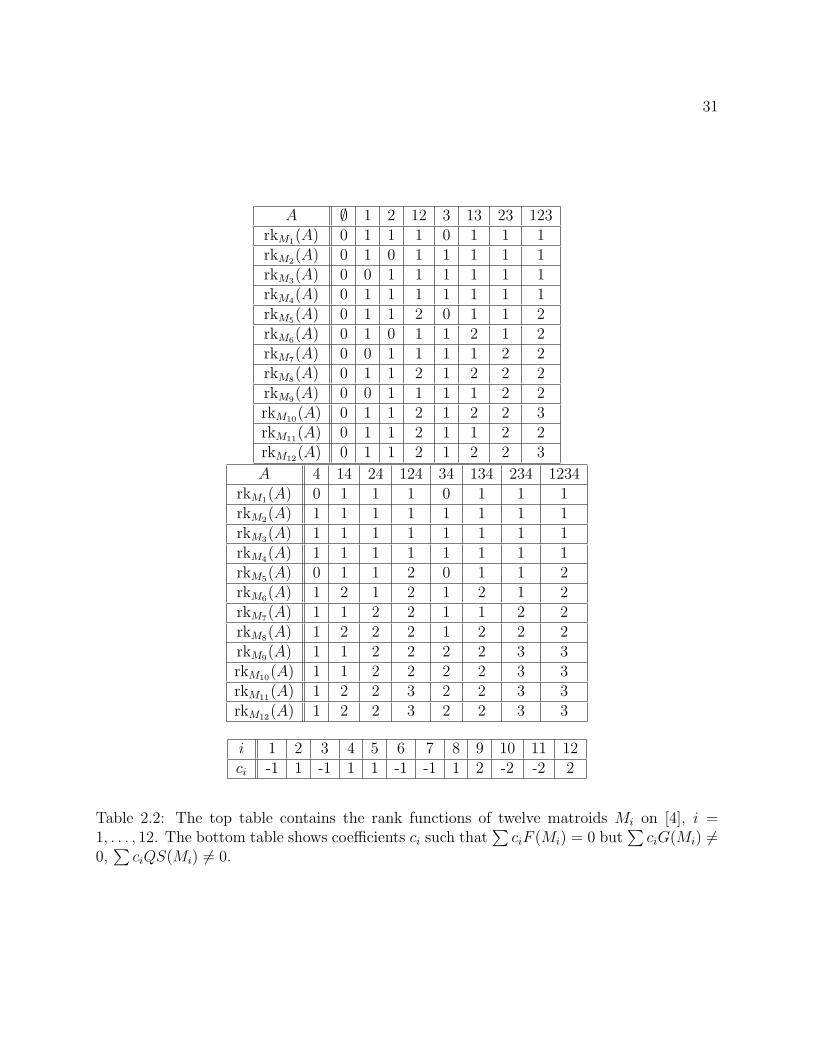
For the remainder of this section, F (M) will denote the function of our Theorem 2.5.1.Since F (M) is not a matroid invariant, it cannot be a specialisation of gM(t), QS(M), orG(M). As one would expect, G(M) and QS(M) are not specialisations of F (M). One linearcombination that certifies this is set out in Table 2.2, in which, to facilitate carrying out therelevant checks for F (M), the relevant matroids are specified via their rank functions.
However, one can give a valuation which is similar in spirit to our F (M) and specialisesto Derksen’s G(M). This valuation will play a significant role in Chapter 3, where it is shownuniversal for matroid valuations. (It will be handled not as a single function s as below, butas its coordinates. The sA,r of Chapter 3 is the coefficient of
((A1, r(A1)), . . . , (An, r(An))
)below.)
Proposition 2.6.1. The function s : Mat→ Gn defined by
s(M) =∑A
((A1, r(A1)), . . . , (An, r(An))
),
where A = (A1, . . . , An) ranges over all maximal flags of M , is a valuation.
Proof. The proof is a straightforward extension of our argument for Theorem 2.5.1. Withthe notation of that proof, checking whether a matroid M satisfies rkM(Ai) = ri for somefixed vector r = (ri), i.e. whether the term ((A1, r1), . . . , (An, rn)) is present in s(M), isequivalent to checking that Poly(M) intersects PAi,ri
and not PAi,ri+1 for each i.
Observe that if Poly(M) intersects PAi,rifor all i then r(Ai) ≥ ri and, since A is a flag,
we can choose a single basis of M whose intersection with Ai has at least ri elements foreach i. Therefore Poly(M) intersects PA1,r1 ∩ · · · ∩ PAn,rn .
Consider the sum ∑(−1)e1+...+eniPA,r+e
(M) (2.6.1)
where the sum is over all e = (e1, ..., en) ∈ 0, 1n, and where PA,r+e is the intersectionPA1,r1+e1 ∩ · · · ∩ PAn,rn+en . By our previous observation this sum equals(∑
e1
(−1)e1iPA1,r1+e1(M)
)· · ·
(∑en
(−1)eniPAn,rn+en(M)
),
which is 1 if the term ((A1, r1), . . . , (An, rn)) is present in s(M), and is 0 otherwise. All theterms in (2.6.1) are valuations, hence s is a valuation.
31
A ∅ 1 2 12 3 13 23 123rkM1(A) 0 1 1 1 0 1 1 1rkM2(A) 0 1 0 1 1 1 1 1rkM3(A) 0 0 1 1 1 1 1 1rkM4(A) 0 1 1 1 1 1 1 1rkM5(A) 0 1 1 2 0 1 1 2rkM6(A) 0 1 0 1 1 2 1 2rkM7(A) 0 0 1 1 1 1 2 2rkM8(A) 0 1 1 2 1 2 2 2rkM9(A) 0 0 1 1 1 1 2 2rkM10(A) 0 1 1 2 1 2 2 3rkM11(A) 0 1 1 2 1 1 2 2rkM12(A) 0 1 1 2 1 2 2 3
A 4 14 24 124 34 134 234 1234rkM1(A) 0 1 1 1 0 1 1 1rkM2(A) 1 1 1 1 1 1 1 1rkM3(A) 1 1 1 1 1 1 1 1rkM4(A) 1 1 1 1 1 1 1 1rkM5(A) 0 1 1 2 0 1 1 2rkM6(A) 1 2 1 2 1 2 1 2rkM7(A) 1 1 2 2 1 1 2 2rkM8(A) 1 2 2 2 1 2 2 2rkM9(A) 1 1 2 2 2 2 3 3rkM10(A) 1 1 2 2 2 2 3 3rkM11(A) 1 2 2 3 2 2 3 3rkM12(A) 1 2 2 3 2 2 3 3
i 1 2 3 4 5 6 7 8 9 10 11 12ci -1 1 -1 1 1 -1 -1 1 2 -2 -2 2
Table 2.2: The top table contains the rank functions of twelve matroids Mi on [4], i =1, . . . , 12. The bottom table shows coefficients ci such that
∑ciF (Mi) = 0 but
∑ciG(Mi) 6=
0,∑ciQS(Mi) 6= 0.

32
Chapter 3
Valuative invariants for polymatroids
This chapter is joint work with Harm Derksen. It is to appear in Advances in Mathematicswith the same title, as doi:10.1016/j.aim.2010.04.016. (This version incorporates some minorchanges, largely for consistency with other chapters.)
3.1 Introduction
Matroids were introduced by Whitney in 1935 (see [94]) as a combinatorial abstractionof linear dependence of vectors in a vector space. Some standard references are [92] and [72].Polymatroids are multiset analogs of matroids and appeared in the late 1960s (see [33, 44]).There are many distinct but equivalent definitions of matroids and polymatroids, for examplein terms of bases, independent sets, flats, polytopes or rank functions. For polymatroids, theequivalence between the various definitions is given in [44]. Here is the definition in termsof rank functions:
Definition 3.1.1. Suppose that X is a finite set (the ground set) and rk : 2X → N =0, 1, 2, . . . , where 2X is the set of subsets of X. Then (X, rk) is called a polymatroid if:
1. rk(∅) = 0;
2. rk is weakly increasing: if A ⊆ B then rk(A) ≤ rk(B);
3. rk is submodular: rk(A ∪B) + rk(A ∩B) ≤ rk(A) + rk(B) for all A,B ⊆ X.
If moreover, rk(x) ≤ 1 for every x ∈ X, then (X, rk) is called a matroid.
An isomorphism ϕ : (X, rkX) → (Y, rkY ) is a bijection ϕ : X → Y such that rkY ϕ =rkX . Every polymatroid is isomorphic to a polymatroid with ground set [d] = 1, 2, . . . , dfor some nonnegative integer d. The rank of a polymatroid (X, rk) is rk(X).
33
Let SPM(d, r) be the set of all polymatroids with ground set [d] of rank r, and SM(d, r) bethe set of all matroids with ground set [d] of rank r. We will write S(P)M(d, r) when we wantto refer to SPM(d, r) or SM(d, r) in parallel. A function f on S(P)M(d, r) is a (poly)matroidinvariant if f
(([d], rk)
)= f
(([d], rk′)
)whenever ([d], rk) and ([d], rk′) are isomorphic. Let
Ssym(P)M(d, r) be the set of isomorphism classes in S(P)M(d, r). Invariant functions on S(P)M(d, r)
correspond to functions on Ssym(P)M(d, r). Let Z(P)M(d, r) and Zsym
(P)M(d, r) be the Z-modules
freely generated by S(P)M(d, r) and Ssym(P)M(d, r) respectively. For an abelian group A, every
function f : S(sym)(P)M (d, r)→ A extends uniquely to a group homomorphism Z
(sym)(P)M (d, r)→ A.
One of the most important matroid invariants is the Tutte polynomial. It was firstdefined for graphs in [88] and generalized to matroids in [18, 24]. This bivariate polynomialis defined by
T((X, rk)
)=∑A⊆X
(x− 1)rk(X)−rk(A)(y − 1)|A|−rk(A).
Regarded as a polynomial in x − 1 and y − 1, T is also known as the rank generatingfunction. The Tutte polynomial is universal for all matroid invariants satisfying a deletion-contraction formula. Speyer defined a matroid invariant in [83] using K-theory. Billera, Jiaand Reiner introduced a quasi-symmetric function F for matroids in [11], which is a matroidinvariant. This quasi-symmetric function is a powerful invariant in the sense that it candistinguish many pairs of non-isomorphic matroids. However, it does not specialize to theTutte polynomial. Derksen introduced in [29] another quasi-symmetric function G whichspecializes to T and F . Let Uα be the basis of the ring of quasi-symmetric functionsdefined in [29]. G is defined by
G((X, rk)
)=∑X
Ur(X),
whereX : ∅ = X0 ⊂ X1 ⊂ · · · ⊂ Xd = X
runs over all d! maximal chains of subsets in X, and
r(X) = (rk(X1)− rk(X0), rk(X2)− rk(X1), . . . , rk(Xd)− rk(Xd−1)).
To a (poly)matroid ([d], rk) one can associate its base polytope Poly(rk) in Rd (see Defi-nition 3.2.2). For d ≥ 1, the dimension of this polytope is ≤ d− 1. The indicator function ofa polytope Π ⊆ Rd is denoted by 1(Π) : Rd → Z. Let P(P)M(d, r) be the Z-module generatedby all 1(Poly(rk)) with ([d], rk) ∈ S(P)M(d, r).
Definition 3.1.2. Suppose that A is an abelian group. A function f : S(P)M(d, r) → A is
strongly valuative if there exists a group homomorphism f : P(P)M(d, r)→ A such that
f(([d], rk)
)= f(1(Poly(rk)))
for all ([d], rk) ∈ S(P)M(d, r).

34
In Section 3.3 we also define a weak valuative property in terms of base polytope decom-positions. Although seemingly weaker, we will show that the weak valuative property isequivalent to the strong valuative property.
Definition 3.1.3. Suppose that d > 0. A valuative function f : S(P)M(d, r) → A is said tobe additive, if f
(([d], rk)
)= 0 whenever the dimension of Poly(rk) is < d− 1.
Most of the known (poly)matroid invariants are valuative. For example, T , F and G allhave this property in common. Speyer’s invariant is not valuative, but does have a similarproperty, which we will call the covaluative property. Valuative invariants and additive in-variants can be useful for deciding whether a given matroid polytope has a decompositioninto smaller matroid polytopes (see the discussion in [11, Section 7]). Decompositions ofpolytopes and their valuations are fundamental objects of interest in discrete geometry intheir own right (see for instance the survey [65]). Matroid polytope decompositions appearedin the work of Lafforgue ([55, 56]) on compactifications of a fine Schubert cell in the Grass-mannian associated to a matroid. The work of Lafforgue implies that if the base polytope ofa matroid does not have a proper decomposition, then the matroid is rigid, i.e., it has onlyfinitely many nonisomorphic realizations over a given field.
Main results
The following theorem proves a conjecture stated in [29]:
Theorem 3.1.4. The G-invariant is universal for all valuative (poly)matroid invariants,i.e., the coefficients of G span the vector space of all valuative (poly)matroid invariants withvalues in Q.
From G one can also construct a universal invariant for the covaluative property whichspecializes to Speyer’s invariant.
It follows from the definitions that the dual P(P)M(d, r)∨ = HomZ(P(P)M(d, r),Z) is thespace of all Z-valued valuative functions on S(P)M(d, r). If P sym
(P)M(d, r) is the push-out of thediagram
Z(P)M(d, r)π(P)M //
1(P)M
Zsym(P)M(d, r)
1sym(P)M
P(P)M(d, r) ρ(P)M
// P sym(P)M(d, r)
(3.1.1)
then the dual space P sym(P)M(d, r)∨ is exactly the set of all Z-valued valuative (poly)matroid
invariants. Let psym(P)M(d, r) be the rank of the free Z-module P sym
(P)M(d, r), and p(P)M(d, r) be
the rank of the free Z-module P(P)M(d, r). Then psym(P)M(d, r) is the number of independent
Z-valued valuative (poly)matroid invariants, and p(P)M(d, r) is the number of independentZ-valued valuative functions on (poly)matroids. We will prove the following formulas:

35
Theorem 3.1.5.
a. psymM (d, r) =
(dr
)and
∑0≤r≤d
psymM (d, r)xd−ryr =
1
1− x− y,
b. psymPM (d, r) =
(r+d−1
r
)if d ≥ 1 or r ≥ 1;
1 if d = r = 0and
∞∑r=0
∞∑d=0
psymPM (d, r)xdyr =
1− x1− x− y
,
c.∑
0≤r≤d
pM(d, r)
d!xd−ryr =
x− yxe−x − ye−y
,
d. pPM(d, r) =
(r + 1)d − rd if d ≥ 1 or r ≥ 1;1 if d = r = 0,
and
∞∑d=0
∞∑r=0
pPM(d, r)xdyr
d!=ex(1− y)1− yex
.
We also will give explicit bases for each of the spaces P(P)M(d, r) and P sym(P)M(d, r) and
their duals (see Theorems 3.5.4, 3.6.3, Corollaries 3.5.5, 3.5.6, 3.6.6, 3.6.5).
The bigraded module
Z(P)M =⊕d,r
Z(P)M(d, r)
has the structure of a Hopf algebra. Similarly, each of the bigraded modules Zsym(P)M, P(P)M
and P sym(P)M has a Hopf algebra structure. The module Zsym
(P)M is the usual Hopf algebra of
(poly)matroids, where multiplication is given by the direct sum of matroids.
In Sections 3.8 and 3.9 we construct bigraded modules T(P)M and T sym(P)M so that T(P)M(d, r)∨
is the space of all additive functions on S(P)M(d, r) and T sym(P)M(d, r)∨ is the space of all additive
invariants. Let t(P)M(d, r) be the rank of T(P )M(d, r) and tsym(P )M(d, r) be the rank of T sym
(P )M(d, r).
Then t(P)M(d, r) is the number of independent additive functions on (poly)matroids, andtsym(P)M(d, r) is the number of independent additive invariants for (poly)matroids. We will
prove the following formulas:
Theorem 3.1.6.
a.∏
0≤r≤d
(1− xd−ryr)tsymM (d,r) = 1− x− y,
b.∏r,d
(1− xdyr)tsymPM (d,r) =
1− x− y1− y
,

36
c.∑r,d
tM(d, r)
d!xd−ryr = log
(x− y
xe−x − ye−y
),
d. tPM(d, r) =
rd−1 if d ≥ 10 if d = 0,
and∑r,d
tPM(d, r)
d!xdyr = log
(ex(1− y)1− yex
).
We will also give explicit bases for the the spaces TM(d, r) and TPM(d, r) in Theo-rem 3.8.6, and of the dual spaces T sym
M (d, r)∨ ⊗Z Q, T symPM (d, r)∨ ⊗Z Q in Theorem 3.10.2.
For Q-valued functions we will prove the following isomorphisms in Section 3.10.
Theorem 3.1.7. Let u0, u1, u2, . . . be indeterminates, where ui has bidgree (1, i). We havethe following isomorphisms of bigraded associative algebras over Q:
a. The space (P symM )∨⊗ZQ of Q-valued valuative invariants on matroids is isomorphic to
Q〈〈u0, u1〉〉, the completion (in power series) of the free associative algebra generated byu0, u1.
b. The space (P symPM )∨⊗ZQ of Q-valued valuative invariants on polymatroids is isomorphic
to Q〈〈u0, u1, u2, . . . 〉〉.
c. The space (T symM )∨ ⊗Z Q of Q-valued additive invariants on matroids is isomorphic to
Qu0, u1, the completion of the free Lie algebra generated by u0, u1.
d. The space (T symPM )∨⊗ZQ of Q-valued additive invariants on polymatroids is isomorphic
to Qu0, u1, u2, . . . .
Tables for p(P)M, psym(P)M, t(P)M, tsym
(P)M are given in Appendix 3.B to this chapter.
An index of notations used in this chapter appears in Appendix 3.C. To aid the readerin keeping them in mind we present an abridged table here. In a notation of the schematicform Lettersuper
sub (d, r):
The letter S refers to the set of *-matroidsZ the Z-module with basis all *-matroidsP the Z-module of indicator functions of *-matroidsT the Z-module of indicator functions of *-matroids,
modulo changes on subspaces of dimension < d− 1with ground set [d] of rank r. Here ∗ stands for one of the prefixes “” or “poly” or “mega”.If the letter is lowercase, we refer not to the Z-module but to its rank.
The subscript M means the *-matroids are matroidsPM polymatroidsMM megamatroids (Def. 3.2.1);

37
additionally, when we want to refer to multiple cases in parallel,
the subscript (P)M covers matroids and polymatroids*M matroids and poly- and mega-matroids.
The superscript sym means that we are only considering *-matroids up to isomorphism.
3.2 Polymatroids and their polytopes
For technical reasons it will be convenient to have an “unbounded” analogue of polyma-troids, especially when we work with their polyhedra. So we make the following definition.
Definition 3.2.1. A function 2X → Z∪ ∞ is called a megamatroid if it has the followingproperties:
1. rk(∅) = 0;
2. rk(X) ∈ Z;
3. rk is submodular: if rk(A), rk(B) ∈ Z, then rk(A∪B), rk(A∩B) ∈ Z and rk(A∪B) +rk(A ∩B) ≤ rk(A) + rk(B).
Obviously, every matroid is a polymatroid, and every polymatroid is a megamatroid.The rank of a megamatroid (X, rk) is the integer rk(X).
By a polyhedron we will mean a finite intersection of closed half-spaces. A polytope is abounded polyhedron.
Definition 3.2.2. For a megamatroid ([d], rk), we define its base polyhedron Poly(rk) as theset of all (y1, . . . , yd) ∈ Rd such that y1 + y2 + · · ·+ yd = rk(X) and
∑i∈A yi ≤ rk(A) for all
A ⊆ X.
If rk is a polymatroid then Poly(rk) is a polytope, called the base polytope of rk. In [33],Edmonds studies a similar polytope for a polymatroid ([d], rk) which contains Poly(rk) as afacet.
Lemma 3.2.3. If ([d], rk) is a megamatroid, then Poly(rk) is nonempty.
Proof. First, assume that rk is a megamatroid such that ri := rk([i]) is finite for i =0, 1, . . . , d. We claim that
y = (r1 − r0, r2 − r1, . . . , rd − rd−1) ∈ Poly(rk).

38
Indeed, if A = i1, . . . , ik with 1 ≤ i1 < · · · < ik ≤ d then, by the submodular property, wehave
∑i∈A
yi =k∑
j=1
(rk([ij])− rk([ij−1])) ≤
≤k∑
j=1
(rk(i1, . . . , ij)− rk(i1, . . . , ij−1)
)= rk(i1, . . . , ik) = rk(A)
where the inequality holds even if the right hand side is infinite.
Now, assume that rk is any megamatroid. Define rkN by
rkN(A) = minX⊆A
rk(X) +N(|A| − |X|). (3.2.1)
Let N be large enough such that rkN([d]) = rk([d]). It may help the reader’s visualization tonote that, in this case, Poly(rkN) is the intersection of Poly(rk) with the orthant (−∞, N ]d.If A,B ⊆ [d], then we have
rkN(A) = rk(X) +N(|A| − |X|), rkN(B) = rk(Y ) +N(|A| − |Y |)
for some X ⊆ A and some Y ⊆ B. It follows that
rkN(A ∩B) + rkN(A ∪B)
≤ rk(X ∩ Y ) +N(|A ∩B| − |X ∩ Y |) + rk(X ∪ Y ) +N(|A ∪B| − |X ∪ Y |)= rk(X ∩ Y ) + rk(X ∪ Y ) +N(|A|+ |B| − |X| − |Y |)≤ rk(X) + rk(Y ) +N(|A|+ |B| − |X| − |Y |) = rkN(A) + rkN(B).
This shows that rkN is a megamatroid. Since rkN(A) ≤ rk(A) for all A ⊆ [d], we havePoly(rkN) ⊆ Poly(rk). Since rkN(A) < ∞ for all A ⊆ [d], we have that Poly(rkN) 6= ∅. Weconclude that Poly(rk) 6= ∅.
A megamatroid ([d], rk) of rank r is a polymatroid if and only if its base polytope iscontained in the simplex
∆PM(d, r) = (y1, . . . , yd) ∈ Rd | y1, . . . , yd ≥ 0, y1 + y2 + · · ·+ yd = r
and it is a matroid if and only if its base polytope is contained in the hypersimplex
∆M(d, r) = (y1, . . . , yd) ∈ Rd | 0 ≤ y1, . . . , yd ≤ 1, y1 + y2 + · · ·+ yd = r.
If ([d], rk) is a matroid, then a subset A ⊆ [d] is a basis when rk(A) = |A| = rk([d]). Inthis case, the base polytope of ([d], rk) is the convex hull of all
∑i∈A ei where A ⊆ [d] is a
basis (see [37]). The base polytope of a matroid was characterized in [37]:

39
Theorem 3.2.4. A polytope Π contained in ∆M(d, r) is the base polytope of a matroid ifand only if it has the following properties:
1. The vertices of Π have integral coordinates;
2. every edge of Π is parallel to ei − ej for some i, j with i 6= j.
We will generalize this characterization to megamatroids. The remainder of this sectionbuilds up to proving Proposition 3.2.9, showing that the following definition captures exactlythe polyhedra Poly(rk) for rk a megamatroid.
Definition 3.2.5. A convex polyhedron contained in y1+· · ·+yd = r is called a megamatroidpolyhedron if for every face F of Π, the linear hull lhull(F ) is of the form z+W where z ∈ Zd
and W is spanned by vectors of the form ei − ej.
The bounded megamatroid polyhedra are exactly the lattice polytopes among the gen-eralized permutohedra of [73] or the submodular rank tests of [69]. General megamatroidpolyhedra are the natural unbounded generalizations.
Faces of megamatroid polyhedra are again megamatroid polyhedra. If we intersect amegamatroid polyhedron Π with the hyperplane yd = s, we get again a megamatroid poly-hedron. For a megamatroid polyhedron Π, define rkΠ : 2[d] → Z ∪ ∞ by
rkΠ(A) := sup∑
i∈A yi | y ∈ Π.
Lemma 3.2.6. Suppose that Π is a megamatroid polyhedron, A ⊆ B and rkΠ(A) <∞. LetF be the face of Π on which
∑i∈A yi is maximal. Then
rkΠ(B) = rkF (B).
Proof. If rkF (B) = ∞ then rkΠ(B) = ∞ and we are done. Otherwise, there exists a faceF ′ of F on which
∑i∈B yi is maximal. Suppose that rkF (B) < rkΠ(B). Define g(y) :=∑
i∈B yi − rkF (B). Then g is constant 0 on F ′, and g(y) > 0 for some y ∈ Π. Therefore,there exists a face F ′′ of Π containing F ′, such that dimF ′′ = dimF ′ + 1 and g(z) > 0for some z ∈ F ′′. Clearly, z 6∈ F and F does not contain F ′′. We have lhull(F ′′) =lhull(F ′) +R(ek − ej) for some k 6= j. By possibly exchanging j and k, we may assume thatF ′′ is contained in lhull(F ′) +R+(ek − ej), where R+ denotes the nonnegative real numbers.Since z ∈ lhull(F ′) + R+(ek − ej) and g(z) > 0 we have k ∈ B and j 6∈ B. In particularj 6∈ A. For all y′′ ∈ F ′′ we can write y′′ = y + r(ek − ej) with y ∈ F and r > 0, and itfollows that
∑i∈A y
′′i ≥
∑i∈A yi = rkΠ(A) since the j-th coordinate of y′′ cannot contribute.
So F ′′ ⊆ F . But this is a contradiction. We conclude that rkF (B) = rkΠ(B).

40
Lemma 3.2.7. Suppose that f(y) =∑d
j=1 αj
∑i∈Xj
yi where
X : ∅ ⊂ X1 ⊂ X2 ⊂ · · · ⊂ Xd = [d]
is a maximal chain, and α1. . . . , αd−1 ≥ 0. For a megamatroid polyhedron Π we have
supy∈Π
f(y) =d∑
j=1
αj rkΠ(Xj).
Proof. First, assume that Π is bounded. Define F0 = Π, and for j = 1, 2, . . . , d, let Fj be theface of Fj−1 for which
∑i∈Xj
yi is maximal. By induction on j and Lemma 3.2.6, we have
that rkFj(Xi) = rkΠ(Xi) for all j < i. Also, Fj is contained in the hyperplane defined by
the equation∑
i∈Xjyi = rkFj−1
(Xj) = rkΠ(Xj). We have Fd = z where z = (z1, . . . , zd) isdefined by the equations ∑
i∈Xj
zi = rkΠ(Xj), j = 1, 2, . . . , d.
It follows that
f(z) =d∑
j=1
αj
∑i∈Xj
zj =d∑
j=1
αj rkΠ(Xj).
Suppose that Π is unbounded. Let ΠN be the intersection of Π with the set y ∈ Rd |yi ≤ N, i = 1, 2, . . . , d. Now ΠN is a bounded megamatroid polyhedron for large positiveintegers N . (For small N , ΠN might be empty.) We have
supy∈Π
f(y) = supN
supy∈ΠN
f(y) = supN
d∑j=1
αj rkΠN(Xj) =
d∑j=1
αj rkΠ(Xj).
Corollary 3.2.8. If Π is a megamatroid polyhedron, then rkΠ is a megamatroid.
Proof. For subsets A,B ⊆ [d], choose a maximal chain X such that Xj = A ∩ B andXk = A ∪B for some j and k, and let
fA(y) =∑i∈A
yi, fB(y) =∑i∈B
yi, f(y) =∑
i∈A∩B
yi +∑
i∈A∪B
yi = fA(y) + fB(y).
By Lemma 3.2.7,
rkΠ(A) + rkΠ(B) = supy∈Π
fA(y) + supy∈Π
fB(y) ≥ supy∈Π
f(y) = rkΠ(A ∩B) + rkΠ(A ∪B).

41
Proposition 3.2.9. A convex polyhedron Π in the hyperplane y1 + y2 + · · · + yd = r is amegamatroid polyhedron if and only if Π = Poly(rk) for some megamatroid rk.
Proof. Suppose that Π is a megamatroid polyhedron. Then rkΠ is a megamatroid by Corol-lary 3.2.8. Clearly we have Π ⊆ Poly(rkΠ). Suppose that f(y) =
∑di=1 αiyi is a linear
function on the hyperplane y1 + · · · + yd = r. Let σ be a permutation of [d] such thatασ(i) ≥ ασ(j) for i < j. Define Xk = σ(1), . . . , σ(k) for k = 1, 2, . . . , d. We can write
f(y) =d∑
j=1
βj
∑i∈Xj
yi,
where βj := ασ(j) − ασ(j+1) ≥ 0 for j = 1, 2, . . . , d− 1 and βd = ασ(d).
By Lemma 3.2.7 we have
supy∈Π
f(y) =d∑
j=1
βj rkΠ(Xj) ≥ supz∈Poly(rkΠ)
d∑j=1
βj
∑i∈Xj
zi = supz∈Poly(rkΠ)
f(z).
Since Π is defined by inequalities of the form f(y) ≤ c, where f is a linear function andc = supy∈Π f(y), we see that Poly(rkΠ) ⊆ Π. We conclude that Poly(rkΠ) = Π.
Conversely, suppose that rk is a megamatroid, and that F is a face of Poly(rk). Choosey in the relative interior of F . Let SF denote the set of all subsets A of [d] for which∑
i∈A yi = rk(A). Note that ∅, [d] ∈ SF . The linear hull of F is given by the equations∑i∈A
yi = rk(A), A ∈ SF .
We claim that SF is closed under intersections and unions. If A,B ∈ SF , then we have( ∑i∈A∩B
yi − rk(A ∩B))
+( ∑
i∈A∪B
yi − rk(A ∪B))
=
=∑i∈A
yi +∑i∈B
yi − rk(A ∩B)− rk(A ∪B) =
rk(A) + rk(B)− rk(A ∩B)− rk(A ∪B) ≥ 0
by the submodular property. Since∑
i∈A∩B yi − rk(A ∩ B) and∑
i∈A∪B yi − rk(A ∪ B) arenonpositive, we conclude that A ∩B,A ∪B ∈ SF and
rk(A) + rk(B) = rk(A ∩B) + rk(A ∪B).
Let us call A ∈ SF prime if A is nonempty and not the union of two proper subsets inSF . Let PF be the set of primes in SF . If C = A ∪B, then∑
i∈C
yi = rk(C)

42
follows from the equations∑i∈A
yi = rk(A),∑i∈B
yi = rk(B),∑
i∈A∩B
yi = rk(A ∩B).
Let C1, C2, . . . , Ck be all prime sets in SF . It follows that the linear hull of F is defined byall the equations ∑
i∈Cj
yi = rk(Cj), j = 1, 2, . . . , k.
Every element of SF is a union of some of the Cj’s. For every j, let Bj be the largestproper subset of Cj which lies in SF . Define Aj = Cj \ Bj and rj = rk(Cj)− rk(Bj). ThenA1 ∪ · · · ∪ Ak = [d] is a partition of [d], and every element of SF is a union of some of theAj’s. The linear hull of F is defined by the equations∑
i∈Aj
yi = rj, j = 1, 2, . . . , k.
Clearly, lhull(F ) contains some integral vector z ∈ Zd and lhull(F ) is equal to z +W whereW is the space spanned by all ei − ej where i, j are such that i, j ∈ Ak for some k.
3.3 The valuative property
There are essentially two definitions of the valuative property in the literature, which wewill refer to as the strong valuative and the weak valuative properties. The equivalence of thesedefinitions is shown in [41] and [91] when valuations are defined on sets of polyhedra closedunder intersection. In this section we will show that the two definitions are equivalent forvaluations defined on megamatroid polytopes. Note that the class of megamatroid polytopesis not closed under intersection: see Example 1.2.1.
Definition 3.3.1. A megamatroid polyhedron decomposition is a decomposition
Π = Π1 ∪ Π2 ∪ · · · ∪ Πk
such that Π,Π1, . . . ,Πk are megamatroid polyhedra, and Πi ∩Πj is empty or contained in aproper face of Πi and of Πj for all i 6= j.
Let SMM(d, r) be the set of megamatroids on [d] of rank r. Let ZMM(d, r) be the Z-modulewhose basis is given by all 〈rk〉 where rk ∈ SMM(d, r).
For a megamatroid polyhedron decomposition
Π = Π1 ∪ Π2 ∪ · · · ∪ Πk

43
we define ΠI =⋂
i∈I Πi if I ⊆ 1, 2, . . . , k. We will use the convention that Π∅ = Π. Define
mval(Π; Π1, . . . ,Πk) =∑
I⊆1,2,...,k
(−1)|I|mI ∈ ZMM(d, r),
where mI = 〈rkI〉 if rkI is the megamatroid with Poly(rkI) = ΠI , and mI = 0 if ΠI = ∅. Wealso define
mcoval(Π; Π1, . . . ,Πk) = 〈rkΠ〉 −∑
F
〈rkF 〉.
where F runs over all interior faces of the decomposition.
Definition 3.3.2. A homomorphism of abelian groups f : ZMM(d, r) → A is called weaklyvaluative, if for every megamatroid polyhedron decomposition
Π = Π1 ∪ Π2 ∪ · · · ∪ Πk
we have f(mval(Π; Π1, . . . ,Πk)) = 0. We say it is weakly covaluative, if for every megamatroidpolyhedron decomposition
Π = Π1 ∪ Π2 ∪ · · · ∪ Πk
we have f(mcoval(Π; Π1, . . . ,Πk)) = 0.
We define a group homomorphism
E : ZMM(d, r)→ ZMM(d, r)
by
E(〈rk〉) =∑
F
〈rkF 〉
where F runs over all faces of Poly(rk) and rkF is the megamatroid with Poly(rkF ) = F .For a polytope Π, we denote the set of faces of Π by face(Π).
Lemma 3.3.3. The homomorphism f : ZMM(d, r)→ A of abelian groups is weakly valuativeif and only if f E is weakly covaluative.
Proof. We have
E(mval(Π; Π1, . . . ,Πk)
)=
∑I⊆1,2,...,k
(−1)|I|E(mI) =
=∑
I⊆1,2,...,k
(−1)|I|∑
F∈face(ΠI)
〈rkF 〉 =∑
F
〈rkF 〉∑
I⊆1,2,...,k;F∈face(ΠI)
(−1)|I|. (3.3.1)

44
Let J(F ) be the set of all indices i such that F is a face of Πi. Suppose that F is a face ofΠ. Then J(F ) = ∅ if and only if F = Π. We have∑
I⊆1,2,...,k;F∈face(ΠI)
(−1)|I| =∑
I⊆J(F )
(−1)|I| =
1 if F = Π;0 if F 6= Π.
If F is an interior face, then J(F ) 6= ∅ and∑I⊆1,2,...,k;F∈face(ΠI)
(−1)|I| =∑
I⊆J(F );I 6=∅
(−1)|I| = −1.
We conclude that
E(mval(Π; Π1, . . . ,Πk)) = 〈rkΠ〉 −∑
F
〈rkF 〉 = mcoval(Π; Π1, . . . ,Πk)
where the sum is over all interior faces F . The lemma follows.
For a polyhedron Π in Rd, let 1(Π) denote its indicator function. Define PMM(d, r) asthe Z-module generated by all 1(Poly(rk)), where rk lies in SMM(d, r).
There is a natural Z-module homomorphism
1MM : ZMM(d, r)→ PMM(d, r)
such that1MM(〈rk〉) = 1(Poly(rk))
for all rk ∈ SMM(d, r).
Definition 3.3.4. A homomorphism of groups f : ZMM(d, r) → A is strongly valuative if
there exists a group homomorphism f : PMM(d, r)→ A such that f = f ψMM.
Suppose that Π = Π1∪ · · · ∪Πk is a megamatroid decomposition. Then by the inclusion-exclusion principle, we have
1MM(mval(Π; Π1, . . . ,Πk)) = 1MM
( ∑I⊆1,2,...,k
(−1)|I|mI
)=
=∑
I⊆1,2,...,k
(−1)|I|∏i∈I
1(Πi) =∑
I⊆1,2,...,k
(−1)|I|1(ΠI) =k∏
i=1
(1(Π)− 1(Πi)) = 0.
This shows that every homomorphism f : ZMM(d, r)→ A of abelian groups with the strongvaluative property has the weak valuative property. In fact the two valuative properties areequivalent by the following theorem:

45
Theorem 3.3.5. A homomorphism f : ZMM(d, r)→ A of abelian groups is weakly valuativeif and only if it is strongly valuative.
The proof of Theorem 3.3.5 is in Appendix 3.A. In view of this theorem, we will fromnow on just refer to the valuative property when we mean the weak or the strong valuativeproperty.
For a megamatroid polytope Π, let Π be the relative interior of Π. Define a homomor-phism 1MM : ZMM(d, r)→ PMM(d, r) by 1MM(〈rk〉) = 1(Q(rk)).
Definition 3.3.6. Suppose that f : ZMM(d, r) → A is a homomorphism of abelian groups.We say that f is strongly covaluative if f factors through 1MM, i.e., there exists a group
homomorphism f such that f = f 1MM.
Corollary 3.3.7. A homomorphism f : ZMM(d, r) → A of abelian groups is weakly covalu-ative if and only if it is strongly covaluative.
Proof. If Π = Π1 ∪ · · · ∪ Πk is a megamatroid polytope decomposition, then
1MM(mcoval(Π; Π1, . . . ,Πk)) = 1MM(〈rkΠ〉)−∑
F
1MM(〈rkF 〉) = 1(Π)−∑
F
1(F ) = 0,
where F runs over all interior faces. This shows that if f has the strong covaluative property,then it has the weak covaluative property.
It is easy to verify that 1MM E = 1MM. Suppose that f is weakly covaluative. ByLemma 3.3.3, f E−1 is weakly valuative. By Theorem 3.3.5, f E−1 is strongly valuative,so f E−1 = f 1MM for some group homomorphism f , and f = f 1MM E = f 1MM.This implies that f is strongly covaluative.
Definition 3.3.8. Suppose that d ≥ 1. A valuative group homomorphism f : ZMM(d, r)→A is additive if f(〈rk〉) = 0 for all megamatroids ([d], rk) for which Poly(rk) has dimension< d− 1.
If f : ZMM(d, r)→ A is additive, then for a megamatroid polyhedron decomposition
Π = Π1 ∪ Π2 ∪ · · · ∪ Πk
we have
f(rkΠ) =k∑
i=1
f(〈rkΠi〉).
A megamatroid polyhedron decomposition Π = Π1 ∪ · · · ∪Πk is a (poly)matroid polytopedecomposition if Π,Π1, . . . ,Πk are (poly)matroid polytopes. Let S(P)M(d, r) be the set of(poly)matroids, and let Z(P)M(d, r) be the free abelian group generated by S(P)M(d, r). We

46
say that f : Z(P)M(d, r) → A has the weak valuative property if f(mval(Π; Π1, . . . ,Πk)) = 0for every (poly)matroid polytope decomposition. We define the weak covaluative propertyfor such homomorphisms f in a similar manner. The group homomorphism E : ZMM(d, r)→ZMM(d, r) restricts to homomorphisms Z(P)M(d, r) → Z(P)M(d, r). A group homomorphismf : Z(P)M(d, r) → A is weakly valuative if and only if f E is weak covaluative. LetP(P)M(d, r) = 1MM(Z(P)M(d, r)) and define 1(P)M : Z(P)M(d, r) → P(P)M(d, r) as the restric-tions of 1MM. A homomorphism f : Z(P)M(d, r) → A is strongly valuative if and only if itfactors through 1(P)M.
Corollary 3.3.9. A homomorphism f : Z(P)M(d, r)→ A is weakly valuative if and only if itis strongly valuative.
Proof. We need to show that ker1(P)M(d, r) = W(P)M(d, r). Clearly W(P)M(d, r) ⊆ker1(P)M(d, r). By Theorem 3.3.5, we have that ker1MM(d, r) = WMM(d, r), soker1(P)M(d, r) = WMM(d, r) ∩ Z(P)M(d, r). Define π(P)M : ZMM(d, r) → Z(P)M(d, r) byπ(P)M(〈rk〉) = 〈rk′〉 where Poly(rk′) = Poly(rk)∩∆(P)M(d, r) if this intersection is nonemptyand π(P)M(〈rk〉) = 0 otherwise. Note that π(P)M is a projection of ZMM(d, r) onto Z(P)M(d, r).We have
π(P)M(mval(Π; Π1, . . . ,Πk)) = mval(Π ∩∆; Π1 ∩∆, . . . ,Πk ∩∆) ∈ W(P)M(d, r),
where ∆ = ∆(P)M(d, r). This shows that π(P)M(WMM(d, r)) ⊆ W(P)M(d, r). We conclude that
ker1(P)M(d, r) = WMM(d, r) ∩ Z(P)M(d, r) ⊆ π(P)M(WMM(d, r)) ⊆ W(P)M(d, r).
The strong covaluative property for a group homomorphism f : Z(P)M(d, r) → A canalso be defined. The proof of Corollary 3.3.7 generalizes to (poly)matroids and f is weaklycovaluative if and only if f is strongly covaluative.
3.4 Decompositions into cones
A chain of length k in [d] is
X : ∅ ⊂ X1 ⊂ · · · ⊂ Xk−1 ⊂ Xk = [d]
(here ⊂ denotes proper inclusion). We will write `(X) = k for the length of such a chain. Ifd > 0 then every chain has length ≥ 1, but for d = 0 there is exactly one chain, namely
∅ = [0]
and this chain has length 0. For a chain X of length k and a k-tuple r = (r1, r2, . . . , rk) ∈(Z ∪ ∞)k, we define a megamatroid polyhedron
RMM(X, r) =
(y1, . . . , yd) ∈ Rd∣∣∣ d∑
i=1
yi = rk, ∀j∑i∈Xj
yi ≤ rj
.

47
We will always use the conventions r0 = 0, X0 = ∅. The megamatroid rkX,r is defined byPoly(rkX,r) = RMM(X, r).
For a megamatroid rk and a chain X of length k we define
RMM(X, rk) = RMM(X, (rk(X1), rk(X2), . . . , rk(Xk))).
Suppose that Π is a polyhedron in Rd defined by gi(y1, . . . , yd) ≤ ci for i = 1, 2, . . . , n,where gi : Rd → R is linear and ci ∈ R. For every face F of Π, the tangent cone ConeF of Fis defined by the inequalities
gi(y1, . . . , yd) ≤ ci
for all i for which the restriction of gi to F is constant and equal to ci.
Theorem 3.4.1 (Brianchon-Gram Theorem [15, 40]). We have the following equality
1(Π) =∑
F
(−1)dim F1(ConeF )
where F runs over all the bounded faces of Π.
For a proof, see [61].
Theorem 3.4.2. For any megamatroid rk : 2[d] → Z ∪ ∞ we have
1(Poly(rk)) =∑X
(−1)d−`(X)1(RMM(X, rk)).
Proof. Assume first that rk(X) is finite for all X ⊆ [d]. We define a convex polyhedronQε(rk) by the inequalities ∑
i∈A
yi ≤ rk(A) + ε(d2 − |A|2)
for all A ⊆ [d] and the equality y1 + · · ·+ yd = r, where r = rk([d]).
Faces of Qε(rk) are given by intersecting Qε(rk) with hyperplanes of the form
HA =
(y1, . . . , yd) ∈ Rd |∑i∈A
yi = rk(A) + ε(d2 − |A|2).
If A,B ⊆ [d], and A and B are incomparable, and (y1, . . . , yd) ∈ HA ∩HB ∩Qε(rk), then∑i∈A
yi +∑i∈B
yi = rk(A) + rk(B) + ε((d2 − |A|2) + (d2 − |B|2))
> rk(A) + rk(B) + ε((d2 − |A ∪B|2) + (d2 − |A ∩B|2))≥ rk(A ∪B) + rk(A ∩B) + ε((d2 − |A ∪B|2) + (d2 − |A ∩B|2))
≥∑
i∈A∪B
yi +∑
i∈A∩B
yi =∑i∈A
yi +∑i∈B
yi

48
This contradiction shows that HA∩HB ∩Qε(rk) = ∅. It follows that all faces are of the form
Fε(X) = Qε(rk) ∩HX1 ∩ · · · ∩HXk−1
where k ≥ 1 andX0 = ∅ ⊂ X1 ⊂ · · · ⊂ Xk−1 ⊂ Xk = [d].
Also, all these faces are distinct.
Let us view Qε(rk) as a bounded polytope in the hyperplane y1 + y2 + · · ·+ yd = r. Fora face Fε(X), its tangent cone ConeFε(X) is defined by the inequalities∑
i∈Xj
yi ≤ rk(Xj) + ε(d2 − |Xj|2)
(and the equality∑d
i=1 yi = r). If X has length k, then the dimension of Fε(X) is d − k.Theorem 3.4.1 implies that
1(Qε(rk)) =∑X
(−1)d−`(X)1(ConeFε(X)).
When we take the limit ε ↓ 0, then 1(Qε(rk)) converges pointwise to 1(Poly(rk)), and1(ConeFε(X)) converges pointwise to 1(RMM(X, rk)).
Finally, for a general polymatroid rk, we have rk = limN→∞ rkN , where rkN is as in theproof of Lemma 3.2.3, and rkN has all ranks finite, and likewise
limN→∞
1(RMM(X, rkN)) = 1(RMM(X, rk)).
So the result follows by taking limits.
Example 3.4.3. To illustrate the proof of Theorem 3.4.2, consider the case where d = 3and r = 3, and rk is defined by rk(1) = rk(2) = rk(3) = 2, rk(1, 2) = rk(2, 3) =rk(1, 3) = 3, rk(1, 2, 3) = 4. The decomposition of Qε(rk) using the Brianchon-Gramtheorem is depicted in Figure 3.1. Note how the summands in the decomposition correspondto the faces of Qε(rk). The dashed triangle is the triangle defined by y1, y2, y3 ≥ 0, y1 + y2 +y3 = 4. Instead of getting cones in the decomposition, we get polygons because we intersectwith this triangle.
In the limit where ε approaches 0 we obtain Figure 3.2. This is exactly the decompositionin Theorem 3.4.2. In this decomposition, the summands do not correspond to the faces ofPoly(rk). ♦

49
+
− −
− − − −
= + + +
+ +
Figure 3.1: A decomposition of Qε(rk), as in Theorem 3.4.2.
3.5 Valuative functions: the groups PM, PPM, PMM
Lemma 3.5.1. The function χ : ZMM(d, r) → Z such that χ(〈rk〉) = 1 for every megama-troid rk has the valuative property.
Proof. LetΠ = Π1 ∪ Π2 ∪ · · · ∪ Πk
be a megamatroid polyhedron decomposition. By Rota’s crosscut theorem [76],
χ(mval(Π; Π1, . . . ,Πk)) =∑
F
µ(Π, F ) = 0,
where F runs over the faces of the decomposition, and µ is the Mobius function.
Lemma 3.5.2. Let H ⊆ Rd be a closed halfspace. Define jH : ZMM(d, r)→ Z by
jH(〈rk〉) =
1 if Poly(rk) ⊆ H,0 otherwise.
Then jH is valuative.

50
+
= + + +
+ + − −
− − − −
Figure 3.2: The limiting decomposition of Poly(rk) corresponding to Figure 3.1.
Proof. LetΠ = Π1 ∪ Π2 ∪ · · · ∪ Πk
be a megamatroid polyhedron decomposition. The intersections of the faces of this decom-position with Rd \ H establish a regular cell complex structure on Π \ H, and a face F ofthe decomposition meets Rd \H if and only if (χ − jH)(rkF ) = 1. It follows that χ − jH isvaluative, by the argument of the previous proof applied to this complex.
Lemma 3.5.2 can also be deduced from the fact that the indicator function of the polardual has the valuative property (see [57]).
Suppose that X is a chain of length k and r = (r1, . . . , rk) is an integer vector withrk = r. Define a homomorphism sX,r : ZMM(d, r)→ Z by
sX,r(rk) =
1 if rk(Xj) = rj for j = 1, 2, . . . , k,0 otherwise.
Proposition 3.5.3. The homomorphism sX,r is valuative.

51
Proof. For ε > 0, define the halfplane H1(ε) by the inequality
k∑j=1
εj−1∑i∈Xj
yi ≤k∑
j=1
εj−1rj
and define H2(ε) byk∑
j=1
εj−1∑i∈Xj
yi ≤k∑
j=1
εj−1rj − εk.
By Lemma 3.2.7 and Lemma 3.5.2, (jH1(ε) − jH2(ε))(rk) = 1 if and only if
k∑j=1
εj−1rj − εk <k∑
j=1
εj−1 rk(Xj) = maxy∈Poly(rk)
k∑j=1
εj−1∑i∈Xj
yi ≤k∑
j=1
εj−1rj (3.5.1)
If (3.5.1) holds for arbitrary small ε, then it is easy to see (by induction on j) that rk(Xj) = rj
for j = 1, 2, . . . , k. From this follows that limε→0 jH1(ε)−jH2(ε) = sX,r. So sX,r is valuative.
Suppose that d ≥ 1. Let pMM(d, r) be the set of all pairs (X, r) such that X is a chainof length k (1 ≤ k ≤ d) and r = (r1, r2, . . . , rk) is an integer vector with rk = r. Wedefine R(P)M(X, r) = RMM(X, r) ∩ ∆(P)M(d, r). If R(P)M(X, r) is nonempty, then it is a(poly)matroid base polytope. Define pPM(d, r) ⊆ pMM(d, r) as the set of all pairs (X, r) with0 ≤ r1 < · · · < rk = r. Let pM(d, r) denote the set of all pairs (X, r) ∈ pMM(d, r) such thatr = (r1, . . . , rk) for some k (1 ≤ k ≤ d),
0 ≤ r1 < r2 < · · · < rk = r
and0 < |X1| − r1 < |X2| − r2 < · · · < |Xk−1| − rk−1 ≤ |Xk| − rk = d− r.
For d = 0, we define pMM(0, r) = pPM(0, r) = pM(0, r) = ∅ for r 6= 0 and pMM(0, 0) =pPM(0, 0) = pM(0, 0) = (∅ ⊆ [0], ()).
Theorem 3.5.4. The group P∗M(d, r) is freely generated by the basis1(R∗M(X, r))
∣∣ (X, r) ∈ p∗M(d, r).
Proof. The case d = 0 is easy, so assume that d ≥ 1.
For megamatroids. If rk is a megamatroid, then 1(Poly(rk)) is an integral combina-tion of functions 1(RMM(X, r)), (X, r) ∈ pMM(d, r) by Theorem 3.4.2. This shows that1(RMM(X, r)), (X, r) ∈ pMM(d, r) generate PMM(d, r). If sX,r(RMM(X ′, r′)) 6= 0 thenrkX′,r′(Xj) = rj for all j, and RMM(X ′, r′) ⊆ RMM(X, r). Suppose that
k∑i=1
ai1(RMM(X(i), r(i))) = 0

52
with k ≥ 1, a1, . . . , ak nonzero integers, and (X(i), r(i)), i = 1, 2, . . . , k distinct. Without lossof generality we may assume that RMM(X(1), r(1)) does not contain RMM(X(i), r(i)) for anyi > 1. We have
0 = sX(1),r(1)
( k∑i=1
aiRMM(X(i), r(i)))
= a1.
Contradiction.
For polymatroids. It is clear that PPM(d, r) is generated by all 1(RPM(X, r)), with (X, r) ∈pMM(d, r). If r1 < 0 then RPM(X, r) is empty. Suppose that ri+1 ≤ ri. It is obvious that
RPM(X, r) = RPM(X ′, r′)
whereX ′ : ∅ = X0 ⊂ X1 ⊂ · · · ⊂ Xi−1 ⊂ Xi+1 ⊂ · · · ⊂ Xk = [d]
andr′ = (r1, r2, . . . , ri−1, ri+1, . . . , rk).
Therefore, PPM(d, r) is generated by all 1(RPM(X, r)) where (X, r) ∈ pPM(d, r). If Π =RPM(X, r) with (X, r) ∈ pPM(d, r), then (X, r) is completely determined by the polytope Π.For 1 ≤ i ≤ d, define ai = maxyi | y ∈ Π. Then r is determined by 0 ≤ r1 < · · · < rk and
r1, . . . , rk = a1, . . . , ad.
The sets Xj, j = 1, 2, . . . , k are determined by Xj = i | ai ≤ rj. This shows thatthe polytopes RPM(X, r), (X, r) ∈ pPM(d, r) are distinct. A similar argument as in themegamatroid case shows that 1(RPM(X, r)), (X, r) ∈ pPM(d, r) are linearly independent.
For matroids. From the polymatroid case it follows that PM(d, r) is generated by all1(RM(X, r)), where (X, r) ∈ pPM(d, r). Suppose that |Xi−1| − ri−1 ≥ |Xi| − ri for somei with 1 ≤ i ≤ k (with the convention that r0 = 0). Then we have
1(RM(X, r)) = 1(RM(X ′, r′))
whereX ′ : ∅ = X0 ⊂ X1 ⊂ · · · ⊂ Xi−1 ⊂ Xi+1 ⊂ · · · ⊂ Xk = [d].
andr = (r1, . . . , ri−1, ri+1, . . . , rk).
This shows that PM(d, r) is generated by all 1(RM(X,r)) where (X, r) ∈ pM(d, r). If Π =RM(X, r) with (X, r) ∈ pM(d, r), then (X, r) is completely determined by the polytope Π.Note that rkΠ(A) = minjrkΠ(Xj)+ |A|−|A∩Xj|. If ∅ ⊂ A ⊂ [d] then A = Xj for some j ifand only if rkΠ(A) < rkΠ(B) for all B with A ⊂ B ⊆ [d] and |A|− rkΠ(A) > |B|− rkΠ(B) forall B with ∅ ⊆ B ⊂ A. So X1, . . . , Xk are determined by Π, and ri = rkΠ(Xj), j = 1, 2, . . . , kare determined as well. This shows that the polytopes RM(X, r), (X, r) ∈ pM(d, r), aredistinct. A similar argument as in the megamatroid case shows that 1(RM(X, r)), (X, r) ∈pM(d, r), are linearly independent.

53
Let (X, r) ∈ pMM(d, r). Consider the homomorphism s≤X,r : ZMM(d, r)→ Z defined by
s≤X,r(rk) =
1 if rk(Xj) ≤ rj for j = 1, 2, . . . , k,0 otherwise.
This homomorphism s≤X,r is a (convergent infinite) sum of several homomorphisms of theform sX′,r′ , so by Proposition 3.5.3 it is valuative.
In view of Theorem 3.5.4, if f : Z(P)M(d, s) → Z is valuative, f is determined by itsvalues on the (poly)matroids R(P)M, since the spaces P(P)M(d, r) are finite-dimensional. Fora (poly)matroid rk, s≤X,r(rk) = 1 if and only if Poly(rk) is contained in Poly(R(P)M(X, r)).Therefore, the matrix specifying the pairing P(P)M(r, d) ⊗ P(P)M(r, d)∨ → Z whose rowscorrespond to the polytopes Poly(R(P)M(X, r)), in some linear extension of the order ofthese polytopes by containment, and whose columns correspond in the same order to s≤X,r,is triangular. The next corollary follows.
Corollary 3.5.5. The group P(P)M(d, r)∨ of valuations Z(P)M(d, r)→ Z has the two basessX,r : (X, r) ∈ p(P)M(d, r)
and
s≤X,r : (X, r) ∈ p(P)M(d, r).
If X is not a maximal chain, then sX,r is a linear combination of functions of the formsX′,r′ where X ′ is a maximal chain. The following corollary follows from Corollary 3.5.5.
Corollary 3.5.6. The group PPM(d, r)∨ of valuations ZPM(d, r) → Z is generated by thefunctions sX,r where X is a chain of subsets of [d] of length d and r = (r1, . . . , rd) is aninteger vector with 0 ≤ r1 ≤ · · · ≤ rd = r.
The generating set of this corollary appeared as the coordinates of the function H definedin §6 of Chapter 2, which was introduced there as a labeled analogue of Derksen’s G.
Proof of Theorem 3.1.5(d). Let a(d, r) be the set of all sequences (a1, . . . , ad) with 0 ≤ ai ≤ rfor all i and ai = r for some i. Clearly |a(d, r)| = (r + 1)d − rd. We define a bijectionf : pPM(d, r)→ a(d, r) as follows. If (X, r) ∈ pPM(d, r), then we define
f(X, r) = (a1, a2, . . . , ad)
where ai = rj and j is minimal such that i ∈ Xj.
Suppose that (a1, . . . , ad) ∈ a(d, r). Let k be the cardinality of a1, . . . , ad. Now r1 <r2 < · · · < rk are defined by
r1, r2, . . . , rk = a1, . . . , ad

54
and for every j, we defineXj = i ∈ [d] | ai ≤ rj.
Then we havef−1(a1, . . . , ad) = (X, r).
A generating function for pPM(d, r) is
∞∑d=0
∞∑r=0
pPM(d, r)xdyr
d!= 1 +
∞∑d=1
∞∑r=0
(r + 1)d − rd
d!xdyr =
= 1 +∞∑
r=0
∞∑d=0
(r + 1)d − rd
d!xdyr = 1 +
∞∑r=0
(e(r+1)x − erx)yr = 1 +ex − 1
1− yex=ex(1− y)1− yex
.
Proof of Theorem 3.1.5(c). Suppose that (X, r) ∈ pM(d, r) has length k. Defineu1, u2, . . . , uk by
u1 = r1, ui = ri − ri−1 − 1 (2 ≤ i ≤ k).
Define v1, v2, . . . , vk by
vi = (|Xi| − ri)− (|Xi−1| − ri−1)− 1 (1 ≤ i ≤ k − 1),
vk = (|Xk| − rk)− (|Xk−1| − rk−1) = d− r − |Xk−1|+ rk−1.
If (X, r) ∈ pM(d, r), then we have that u1, . . . , uk, v1, . . . , vk are nonnegative, and
u1 + · · ·+ uk = r − k + 1, v1 + · · ·+ vk = d− r − k + 1.
Let Yi = Xi\Xi−1 for i = 1, 2, . . . , k. If k ≥ 2, then we have u1+v1+1 = |Y1|, uk+vk+1 = |Yk|and ui + vi + 2 = |Yi| for i = 2, 3, . . . , k − 1. There are
d!
(u1 + v1 + 1)!(u2 + v2 + 2)!(u3 + v3 + 2)! · · · (uk−1 + vk−1 + 2)!(uk + vk + 1)!
partitions of [d] into the subsets Y1, Y2, . . . , Yk, such that (X, r) has the given u and v values.If k = 1, then u1 + v1 = d and d!/(u1 + v1)! = 1 so there is just one pair (X, r) with given uand v values.
This yields the generating function
∞∑d=0
d∑r=0
pM(d, r)
d!xd−ryr =
∑u1,v1≥0
tu1sv1
(u1 + v1)!+
+∑
u1,...,uk≥0v1,...,vk≥0
xu1+u2+···+uk+k−1yv1+v2+···+vk+k−1
(u1 + v1 + 1)!(u2 + v2 + 2)! · · · (uk−1 + vk−1 + 2)!(uk + vk + 1)!(3.5.2)

55
We have that ∑u,v≥0
xuyv
(u+ v)!=
∞∑d=0
∑u+v=d
tusv
d!=
∞∑d=0
xd+1 − yd+1
(x− y)d!=xex − yey
x− y, (3.5.3)
∑u,v≥0
tusv
(u+ v + 1)!=
∞∑d=0
∑u+v=d
xuyv
(d+ 1)!=
∞∑d=0
xd+1 − yd+1
(x− y)(d+ 1)!=
=∞∑
d=1
xd − yd
(x− y)d!=
∞∑d=0
xd − yd
(x− y)d!=ex − ey
x− y, (3.5.4)
and∑u,v≥0
xuyv
(u+ v + 2)!=
∞∑d=0
∑u+v=d
xuyv
(d+ 2)!=
∞∑d=0
xd+1 − yd+1
(x− y)(d+ 2)!=
=∞∑
d=1
xd − yd
(x− y)(d+ 1)!=
(ex − 1)/x− (ey − 1)/y
x− y=yex − y − xey + x
(x− y)xy. (3.5.5)
Using (3.5.3), (3.5.4) and (3.5.5) with (3.5.2) yields
∞∑d=0
d∑r=0
pM(d, r)
d!xd−ryr =
=xex − yey
x− y+ xy
(ex − ey
x− y
)2 ∞∑k=2
(yex − y − xey + x
x− y
)k−2
=
=xex − yey
x− y+
(ex − ey
x− y
)2xy
1− yex − y − xey + x
x− y
=
=xex − yey
x− y+
xy(ex − ey)2
(x− y)(xey − yex)=
x− yxe−x − ye−y
. (3.5.6)
The values of p(P)M(d, r) for small d and r can be found in Appendix 3.B.
3.6 Valuative invariants: the groups P symM , P sym
PM , P symMM
Let YMM(d, r) be the group generated by all formal differences 〈rk〉 − 〈rk σ〉 where rk :2[d] → Z ∪ ∞ is a megamatroid of rank r and σ is a permutation of [d]. We define

56
ZsymMM(d, r) = ZMM(d, r)/YMM(d, r). Let πMM : ZMM(d, r) → Zsym
MM(d, r) be the quotienthomomorphism. If rkX : 2X → Z∪∞ is any megamatroid, then we can choose a bijectionϕ : [d] → X, where d is the cardinality of X. Let r = rkX(X). The image of 〈rkX ϕ〉 inZsym
MM(d, r) does not depend on ϕ, and will be denoted by [rkX ]. The megamatroids (X, rkX)and (Y, rkY ) are isomorphic if and only if [rkX ] = [rkY ]. So we may think of Zsym
MM(d, r) asthe free group generated by all isomorphism classes of rank r megamatroids on sets with delements.
Let BMM(d, r) be the group generated by all 1(Poly(rk)) − 1(Poly(rk σ)) where rk :2[d] → Z∪∞ is a megamatroid of rank r and σ is a permutation of [d]. Define P sym
MM (d, r) =PMM(d, r)/BMM(d, r) and let ρMM : PMM(d, r)→ P sym
MM (d, r) be the quotient homomorphism.From the definitions it is clear that 1MM(YMM(d, r)) = BMM(d, r). Therefore, there exists aunique group homomorphism
1symMM : Zsym
MM(d, r)→ P symMM (d, r)
such that the following diagram commutes:
ZMM(d, r)1MM //
πMM
PMM(d, r)
ρMM
Zsym
MM(d, r)1symMM
// P symMM (d, r).
(3.6.1)
This diagram is a push-out. Define Y(P)M(d, r) = YMM(d, r) ∩ Z(P)M(d, r). The groupY(P)M(d, r) is the group generated by all 〈rk〉−〈rk σ〉 where rk : 2[d] → N is a (poly)matroidof rank r and σ is a permutation of [d]. Define Zsym
(P)M(d, r) = Z(P)M(d, r)/Y(P)M(d, r). The
group Zsym(P)M(d, r) is freely generated by all [rk] where rk : X → N is a ∗matroid of rank r
and d = |X|.Define B∗M(d, r) as the group generated by all 1(Poly(rk)) − 1(Poly(rk σ)) where
rk : 2[d] → N is a ∗matroid of rank r and σ is a permutation of [d]. Let P sym∗M (d, r) =
P∗M(d, r)/B∗M(d, r).
Lemma 3.6.1. We have
B(P)M(d, r) = BMM(d, r) ∩ P(P)M(d, r).
Proof. Define q(P)M : PMM(d, r) → P(P)M(d, r) by q(P)M(f) = f · 1(∆(P)M(d, r)). Thisis well defined because for any megamatroid rk : 2[d] → Z ∪ ∞ of rank r, wehave q(P)M(1(Poly(rk))) = 1(Poly(rk)) · 1(∆(P)M(d, r)) = 1(Poly(rk) ∩ ∆(P)M(d, r)) andPoly(rk) ∩ ∆(P)M(d, r) is either empty or a polymatroid polyhedron. Clearly, q(P)M is aprojection of PMM(d, r) onto P(P)M(d, r). Since q(P)M(BMM(d, r)) ⊆ B(P)M(d, r), it followsthat
BMM(d, r) ∩ P(P)M(d, r) = qPM(BMM(d, r) ∩ P(P)M(d, r)) ⊆ B(P)M(d, r).
It follows that BMM(d, r) ∩ P(P)M(d, r) = B(P)M(d, r).

57
By restriction, we get also the commutative push-out diagrams (3.1.1) from the introduc-tion. Define psym
∗M (d, r) as the set of all pairs (X, r) ∈ p∗M(d, r) such that for every j, thereexists an i such that
Xj = [i] = 1, 2, . . . , i.
Define A∗M(d, r) as the Z module generated by all 1(R∗M(X, r)) with (X, r) ∈ psym∗M (d, r).
Lemma 3.6.2. We have
P∗M(d, r) = A∗M(d, r)⊕B∗M(d, r).
Proof. By the definitions of A∗M(d, r) and B∗M(d, r) it is clear that P∗M(d, r) =A∗M(d, r) + B∗M(d, r). Consider the homomorphism τ : P∗M(d, r) → P∗M(d, r) de-fined by τ(f) =
∑σ f σ where σ runs over all permutations of [d]. Clearly,
B∗M(d, r) is contained in the kernel of τ . Recall that 1(R∗M(X, r)), (X, r) ∈p∗M(d, r) is a basis of P∗M(d, r). From this it easily follows that the setτ(1(R∗M(d, r))), (X, r) ∈ psym
∗M (d, r) is independent over Q. Therefore the restriction of τto A∗M(d, r) is injective and A∗M(d, r) ∩B∗M(d, r) = 0.
Theorem 3.6.3. The Z-module P sym?M (d, r) is freely generated by all ρ?M(1(R?M(X, r))) with
(X, r) in psym?M (d, r).
Proof. It is clear that ρ∗M(A∗M(d, r)) = P sym∗M (d, r). So the restriction is surjective. It is also
injective by Lemma 3.6.2. So the restriction of ρ∗M : P∗M(d, r) → P sym∗M (d, r) to A∗M(d, r)
is an isomorphism. From the definition of A?M(d, r) it follows that the given set generatesP sym
?M (d, r), and the set is independent because of Theorem 3.5.4.
The matroid polytopes RM(X, r) are the polytopes of Schubert matroids and their imagesunder relabeling the ground set. Schubert matroids were first described by Crapo [23], andhave since arisen in several contexts. So Theorem 3.6.3 says that the indicator functions ofSchubert matroids form a basis for P sym
M (d, r).
Recall that Zsym∗M can be viewed as the free Z-module generated by all isomorphism classes
of ∗matroids on a set with d elements of rank r. We say that a group homomorphismf : Zsym
MM(d, r)→ A is valuative if and only if f πMM is valuative. For any (X, r) ∈ pMM(d, r)and σ a permutation of [d], we have sX,r(rk σ) = sσX,r(rk), where σ acts on X by permutingeach set in the chain. So the symmetric group Sd acts naturally on P∗M(d, r). It is easy tosee that
P sym?M (d, r)∨ ∼=
(P?M(d, r)∨
)Sd ,
where the right-hand side is the set of Sd-invariant elements of P?M(d, r)∨.
For (X, r) ∈ psymMM(d, r), define a homomorphism ssym
X,r : ZMM(d, r)→ Z by
ssymX,r =
∑σX
sσX,r

58
where the sum is over all chains σX in the orbit of X under the action of the symmetricgroup. Then Corollary 3.5.5 implies the following.
Corollary 3.6.4. The Q-vector space P sym(P)M(d, r)∨ ⊗Z Q of valuations Zsym
(P)M(d, r) → Q has
a basis given by the functions ssymX,r for (X, r) ∈ psym
(P)M(d, r).
For a sequence α = (α1, . . . , αd) of nonnegative integers with |α| =∑
i αi = r, we define
uα = sX,r : Zsym(P)M(d, r)→ Z,
where X i = [i] for i = 1, 2, . . . , r and r = (α1, α1 + α2, . . . , α1 + · · · + αd). Parallel toCorollary 3.5.6 we also have the following.
Corollary 3.6.5. The Q-vector space P symPM (d, r)∨ ⊗Z Q of valuations Zsym
PM (d, r)→ Q has aQ-basis given by the functions uα, where α runs over all sequences (α1, . . . , αd) of nonnegativeintegers with |α| = r.
Corollary 3.6.6. The Q-vector space P symM (d, r)∨ ⊗Z Q of valuations Zsym
M (d, r)→ Q has aQ-basis given by all functions uα where α runs over all sequences (α1, . . . , αd) ∈ 0, 1d with|α| = r.
Proof of Theorem 3.1.4. From the definitions of the Uα and the uα, it follows that uα(〈rk〉) isthe coefficient of Uα in G(〈rk〉). In other words, uα is a dual basis to Uα. The universalityfollows from Corollary 3.6.6.
The rank of P sym(P)M(d, r) is equal to the cardinality of psym
(P)M(d, r). If (X, r) and `(X) = k
lies in psym(P)M(d, r) then X is completely determined by the numbers si := |Xi|, 1 ≤ i ≤ k.
Proof of Theorem 3.1.5(b). Given k, there are(
rk−1
)ways of choosing r = (r1, . . . , rk) with
0 < r1 < r2 < · · · < rk = r and(
d−1k−1
)ways of choosing (s1, . . . , sk) with 0 < s1 < s2 < · · · <
sk = d. So the cardinality of psymPM (d, r) is∑
k≥1
(r
k − 1
)(d− 1
k − 1
)=∑k≥0
(r
k
)(d− 1
k
)=
(r + d− 1
r
).
∑r,d
psymPM (d, r)xdyr =
∑r,d
(r+d−1
r
)xdyr =
∑d
(1− x)−dyd =1
1− y1−x
=1− x
1− x− y.

59
Proof of Theorem 3.1.5(a). Let ti = si − ri. Then we have 0 < t1 < t2 < · · · < tk−1 ≤ tk =d− r. Given k, there are
(r
k−1
)ways of choosing r such that 0 ≤ r1 < · · · < rk = r and
(d−rk−1
)ways of choosing (t1, . . . , tk) with 0 < t1 < · · · < tk−1 ≤ tk = d − r. So the cardinality ofpsym
M (d, r) is ∑k≥1
(r
k − 1
)(d− rk − 1
)=∑k≥0
(r
k
)(d− rk
)=
(d
r
).
So we have ∑r,d
psymM (d, r)xd−ryr =
∑d
(x+ y)d =1
1− x− y.
Example 3.6.7. Consider polymatroids for r = 2 and d = 3. All polymatroid base polytopesare contained in the triangle
(y1, y2, y3) ∈ R3 | y1 + y2 + y3 = 2, y1, y2, y3 ≥ 0.
020200
002
101 011
110
There are(
d−1+rr
)=(42
)elements in our distinguished basis psym
PM (3, 2) and the polytopesR(X, r), (X, r) ∈ psym
PM (3, 2) are given by:
1 3 3
3 3 6
These 6 polytopes correspond to the following pairs (X, r) ∈ pPM(3, 2).
X : 1, 2, 3 X : 1, 2 ⊂ 1, 2, 3 X : 1 ⊂ 1, 2, 3r = (2) r = (1, 2) r = (1, 2)X : 1 ⊂ 1, 2, 3 X : 1, 2 ⊂ 1, 2, 3 X : 1 ⊂ 1, 2 ⊂ 1, 2, 3r = (0, 2) r = (0, 2) r = (0, 1, 2)

60
The symmetric group S3 acts on the triangle by permuting the coordinates y1, y2, y3.
If S3 acts on the generators R(X, r) with (X, r) ∈ pPM(3, 2), then we get all R(X, r)with (X, r) ∈ pPM(3, 2). In the figure, we wrote for each polytope the cardinality of the orbitunder S3. The cardinality of pPM(3, 2) is 1 + 3 + 3 + 3 + 3 + 6 = 19. This is consistent withTheorem 3.1.5, because the cardinality is (r + 1)d − rd = 33 − 23 = 19.
♦Example 3.6.8. Consider matroids for r = 2 and d = 4. All matroid base polytopes arecontained in the set
(y1, y2, y3, y4) ∈ R4 | y1 + y2 + y3 + y4 = 2, ∀i 0 ≤ yi ≤ 1.This set is an octahedron:
1010
0101
0110
1001
0011
1100
There are(
dr
)=(42
)elements in pM(4, 2), and the polytopes RM(X, r), (X, r) ∈ pM(4, 2)
are given by:
124 6
1 6 4
These 6 polytopes correspond to the following pairs (X, r) ∈ pM(4, 2).
X : 1, 2, 3, 4 X : 1, 2 ⊂ 1, 2, 3, 4 X : 1, 2, 3 ⊂ 1, 2, 3, 4r = (2) r = (1, 2) r = (1, 2)X : 1 ⊂ 1, 2, 3, 4 X : 1, 2 ⊂ 1, 2, 3, 4 X : 1 ⊂ 1, 2, 3 ⊂ 1, 2, 3, 4r = (0, 2) r = (0, 2) r = (0, 1, 2)

61
The symmetric group S4 acts by permuting the coordinates y1, y2, y3, y4. This groupacts on the octahedron, but it is not the full automorphism group of the octahedron. Alsonote that not all elements of S4 preserve the orientation. If S4 acts on the generatorsRM(X, r) with (X, r) ∈ pM(4, 2), then we get all R(X, r) with (X, r) ∈ pM(4, 2). In thefigure, we write for each polytope the cardinality of the orbit under S4. The cardinality ofpM(4, 2) is 1 + 6 + 4 + 4 + 6 + 12 = 33, which is compatible with Theorem 3.1.5 and thetable in Appendix 3.B. Besides the polytopes R(X, r), (X, r) ∈ pM(4, 2), there are 3 morematroid base polytopes (belonging to isomorphic matroids), but these decompose as follows.
−
= +
♦
3.7 Hopf algebra structures
Define Z∗M =⊕
d,r Z∗M(d, r), and in a similar way define Zsym∗M , P∗M, and P sym
∗M . We canview Z∗M as the Z-module freely generated by all isomorphism classes of ∗matroids.
If rk1 : 2[d] → Z ∪ ∞ and rk2 : 2[e] → Z ∪ ∞ then we define
rk1 rk2 : 2[d+e] → Z ∪ ∞
by(rk1 rk2)(A) = rk1(A ∩ [d]) + rk2(i ∈ [e] | d+ i ∈ A)
for any set A ⊆ [d+ e]. Note that is not commutative. We have a homomorphism
∇ : ZMM(d, r)⊗Z ZMM(e, s)→ ZMM(d+ e, r + s).
defined by∇(〈rk1〉 ⊗ 〈rk2〉) = 〈rk1 rk2〉.
The multiplication ∇ : ZMM ⊗Z ZMM → ZMM makes ZMM(d, r) into an associative (non-commutative) ring with 1. The unit η : Z → ZMM(d, r) is given by 1 7→ 〈rk0〉 whererk0 : 2[0] → Z ∪ ∞ is the unique megamatroid defined by rk(∅) = 0. With this multiplica-tion, ZM(d, r) and ZPM(d, r) are subrings of ZMM(d, r). The multiplication also respects thebigrading of ZMM(d, r).
Next, we define a comultiplication for ZMM. Suppose that X = i1, i2, . . . , id is a setof integers with i1 < · · · < id and rk : 2X → Z ∪ ∞ is a megamatroid. We define a
megamatroid rk : 2[d] → Z ∪ ∞ by rk(A) = rk(ij | j ∈ A). If rk : 2X → Z ∪ ∞ is

62
a megamatroid and B ⊆ A ⊆ X then we define rkA/B : 2A\B → Z ∪ ∞ by rkA/B(C) =rk(B ∪ C)− rk(B) for all C ⊆ A \B. We also define rkA := rkA/∅ and rk/B = rkX/B.
We now define∆ : ZMM → ZMM ⊗Z ZMM
by
∆(〈rk〉) =∑
A⊆[d]; rk(A)<∞
〈rkA〉 ⊗ 〈rk/A〉.
where A runs over all subsets of [d] for which rk(A) is finite. This comultiplication iscoassociative, but not cocommutative. If rk : 2[d] → Z ∪ ∞ is a megamatroid, then thecounit is defined by
ε(〈rk〉) =
1 if d = 0;0 otherwise.
The reader may verify that the multiplicative and comultiplicative structures are compatible,making ZMM into a bialgebra. Note that ∆ also restricts to comultiplications for ZPM andZM, and ZPM and ZM are sub-bialgebras of ZMM.
We define a group homomorphism S : ZMM → ZMM by
S(〈rk〉) =d∑
r=1
(−1)r∑
X; `(X)=r,rk(X1)<∞,...,rk(Xr)<∞
r∏i=1
〈 rkXi/Xi−1〉.
Here we use the convention X0 = ∅. One can check that S makes ZMM into a Hopf algebra.Restriction of S makes ZM and ZPM into sub-Hopf algebras of ZMM. We conclude that Z∗Mhas the structure of bigraded Hopf algebras over Z.
It is well known that ZsymM has the structure of a Hopf algebra over Z. Similarly we have
that ZsymMM and Zsym
PM have a Hopf algebra structure. The multiplication
∇ : ZsymMM ⊗Z Z
symMM → Zsym
MM
is defined by∇([rk1]⊗ [rk2]) = [rk1⊕ rk2].
The comultiplication is defined by
∆([rk]) =∑
A⊆X;rk(A)<∞
[(A, rkA)]⊗ [(X \ A, rk/A)]
for any megamatroid rk : 2X → Z ∪ ∞. The unit η : Z → ZsymMM is given by 1 7→ [(∅, rk0)]
and the counit ε : ZsymMM → Z is defined by
ε([(X, rk)]) =
1 if X = ∅;0 otherwise.

63
Finally, we define the antipode S : ZsymMM → Zsym
MM by
S([rk]) =d∑
r=1
(−1)r∑
X; `(X)=r,rk(X1)<∞,...,rk(Xr)<∞
r∏i=1
[(Xi \Xi−1, rkXi/Xi−1)].
From the definitions, it is clear that the π∗M are Hopf algebra morphisms.
The space PMM inherits a Hopf algebra structure from ZMM. We define the multiplication∇ : PMM ⊗ PMM → PMM by
∇(1(Π1)⊗ 1(Π2)) = 1(Π1 × Π2). (3.7.1)
It is easy to verify that ∇ (1MM ⊗ 1MM) = 1MM ∇.
To define the comultiplication ∆ : PMM → PMM ⊗ PMM, we would like to have that(ψMM⊗ψMM)⊗∆ = ∆ψMM. So for a megamatroid polytope rk : 2[d] → Z∪∞ we wouldlike to have
∆(1(Poly(rk))) = ∆(ψMM(〈rk〉)) =∑
A⊆[d];rk(A)<∞
ψMM(rkA)⊗ ψMM(rk/A) =
=∑
A⊆[d];rk(A)<∞
1(Poly(rkA))⊗ 1(Poly(rk/A)).
A basis of PMM is given by all RMM(X, r), with (X, r) ∈ pMM =⋃
d,r pMM(d, r). Recallthat the rank function rkX,r is defined such that Poly(rkX,r) = RMM(X, r). We have thatrkX,r(A) <∞ if and only if A = Xi for some i. In this case we have
∆(〈rkX,r〉) =k∑
i=0
〈rkXi,ri〉 ⊗ 〈rkXi,ri〉,
whereX i : ∅ ⊂ X1 ⊂ · · · ⊂ Xi, ri = (r1, r2, . . . , ri)
X i : ∅ ⊂ Xi+1 \Xi ⊂ · · · ⊂ Xk \Xi, ri = (ri+1 − ri, . . . , rk − ri).
We define ∆ by
∆(1(RMM(X, r))) =k∑
i=0
1(RMM(X i, ri))⊗ 1(RMM
(X i, ri)).

64
From this definition and Theorem 3.4.2 follows that
∆(1(Poly(rk))) =∑X
(−1)d−`(X)∆1(RMM(X, rk)) =
=∑X
`(X)∑i=0
(−1)|Xi|−i1(RMM(X i, rkXi
))⊗ (−1)d−|Xi|−`(X)+i1(RMM(X i, rk/Xi
)) =
=∑
A⊆[d];rk(A)<∞
1(Poly(rkA))⊗ 1(Poly(rk/A)). (3.7.2)
In a similar fashion we can define the antipode S : PMM → PMM.
The Hopf algebra structure on PMM naturally induces a Hopf algebra structure on P symMM
such that ρMM and 1symMM are Hopf algebra homomorphisms. Also PPM is a Hopf subalgebra
of PMM and PM is a Hopf subalgebra of PPM. Similarly P symPM is a Hopf subalgebra of P sym
MM ,and P sym
M is a Hopf subalgebra of P symPM .
As a first observation to motivate the consideration of these Hopf algebra structures, weconsider multiplicative invariants.
Definition 3.7.1. A multiplicative invariant for ∗matroids with values in a commutativering A (with 1) is a ring homomorphism f : Zsym
∗M → A.
That is to say, f is multiplicative if f(rk1⊕ rk2) = f(rk1)f(rk2). This is exactly thecondition that f be a group-like element of the graded dual algebra P sym
M (d, r)#. Many(poly)matroid invariants of note have this property, for instance the Tutte polynomial.
Proposition 3.7.2. The Tutte polynomial T ∈ P symM (d, r)# is given by
T = e(y−1)u0+u1eu0+(x−1)u1 . (3.7.3)
Proof. Recall the definition of uα in terms of rank conditions on a chain of sets. In viewof (3.7.2), we have that the multiplication in (P sym
∗M )# is given by uα · uβ =(
d+ed
)uαβ, where
α has length d and β has length e. Denote the right side of (3.7.3) by f . We have
f =∞∑i=0
∞∑j=0
(i+ j)!
i!j!((y − 1)u0 + u1)
i(u0 + (x− 1)u1)j
=∑
i
∑j
(i+ j)!
i!j!
∑α∈0,1i+j
(x− 1)ri+j−ri(y − 1)i−ri (i+ j)!uα
where ri =∑i
k=1 αk, so that i− ri is the number of indices 1 ≤ k ≤ i such that αk = 0, andri+j − ri is the number of indices i+ 1 ≤ k ≤ j such that αk = 1.

65
Let d = i + j. For a matroid rk on [d] of rank r, the elements rk and 1/d!∑
σ∈Sdrk σ
of ZM(d, r) have equal image under πM. Therefore
f(rk) =1
d!
∑σ∈Sd
f(rk σ)
=1
d!
∑σ∈Sd
∑i+j=d
d!
i!j!
∑α∈0,1d
(x− 1)rd−ri(y − 1)i−ri uα(rk σ)
=∑σ∈Sd
∑i+j=d
1
i!j!(x− 1)r−rk(σ([i]))(y − 1)i−rk(σ([i])).
The set σ([i]) takes each value A ⊆ [d] in |A|!(d− |A|)! ways, so
f(rk) =∑A⊆[d]
(x− 1)r−rk(A)(y − 1)|A|−rk(A) = T (rk).
3.8 Additive functions: the groups TM, TPM, TMM
For 0 ≤ e ≤ d we define P∗M(d, r, e) ⊆ P∗M(d, r) as the span of all 1(Π) where Π ⊆ Rd is a∗matroid polytope of dimension ≤ d−e. We have P∗M(0, r, 0) = P∗M(0, r) and P∗M(d, r, 1) =P∗M(d, r) for d ≥ 1. These subgroups form a filtration
· · · ⊆ P∗M(d, r, 2) ⊆ P∗M(d, r, 1) ⊆ P∗M(d, r, 0) = P∗M(d, r).
Define P ∗M(d, r, e) := P∗M(d, r, e)/P∗M(d, r, e+1). If Π1 and Π2 are polytopes of codimensione1 and e2 respectively, then Π1 × Π2 has codimension e1 + e2. It follows from (3.7.1) thatthe multiplication ∇ respects the filtration. Since Poly(rkA) × Poly(rk/A) is contained inPoly(rk), it follows from (3.7.2) that the comultiplication ∆ also respects the filtration:
∆(P∗M(d, r, e)) ⊆∑i,j,k
P∗M(i, j, k)⊗ P∗M(d− i, r − j, e− k)
Similarly, the antipode S respects the grading. The associated graded algebra
P ∗M =⊕d,r,e
P ∗M(d, r, e)
has an induced Hopf algebra structure. We define T?M(d, r) = P ?M(d, r, 1).
For every partition X : [d] =∐e
i=1Xi into nonempty subsets there exists a natural map
ΦX :∏
i
RXi → Rd

66
DefineP∗M(X) =
⊕r1,r2,...,re∈Z
P∗M(|X1|, r1)⊗ · · · ⊗ P∗M(|Xe|, re)
andP ∗M(X) =
⊕r1,r2,...,re∈Z
T∗M(|X1|, r1)⊗ · · · ⊗ T∗M(|Xe|, re).
The map ΦX induces a group homomorphism
φX : P∗M(X, e)→ P∗M(d, r, e)
defined by
φX(1(Π1)⊗ 1(Π2)⊗ · · · ⊗ 1(Πe)) = 1(ΦX(Π1 × Π2 × · · · × Πe)).
The map φX induces a group homomorphism
φX : P ∗M(X, e)→ P ∗M(d, r, e).
A vector y = (y1, . . . , yd) ∈ Rd is called X-integral if∑
i∈Xjyi ∈ Z for j = 1, 2, . . . , e.
An X-integral vector y is called X-regular, if for every j and every Y ⊆ Xj we have: if∑i∈Y yi ∈ Z, then Y = ∅ or Y = Xj. In other words, an X-integral vector y is called
X-regular if it is not integral for any refinement of X. We call y X-balanced if∑
i∈S yi = 0holds if and only if S is a union of some of the Xj’s.
Choose an X-balanced vector yX for every X. For f ∈ P∗M(d, r) we define
γX(f)(x) := limε↓0
f(x+ εyX).
If Π is a ∗matroid base polytope, then γX(1(Π))(x) is constant on faces of Π. This showsthat γX(1(Π)) ∈ P∗M(d, r). So γX is an endomorphism of P∗M(d, r). Now γX also inducesan endomorphism γX of P ∗M(d, r).
Lemma 3.8.1. We have that γX γX = γX .
Proof. Suppose that x ∈ Rd. Consider the set S of all x + εyX with ε ∈ R. There exista partition Y of [d] and a dense open subset U of S such that all points in U are Y -regular. Then there exists a δ > 0 such that T = x + εy | 0 < ε < δ has only Y -regularpoints. For every ∗matroid base polytope Π, we have that T ∩ Π = ∅ or T ⊆ Π. Itfollows that for every f ∈ PM∗(d, r) there exists a constant c such that f is equal to c onT . Therefore γX(f)(x) = c and γX(f) is constant and equal to c on T . We conclude thatγX(γX(f))(x) = c = γX(f)(x).

67
Lemma 3.8.2. Suppose that X, Y are partitions of [d] into e nonempty subsets, and X 6= Y .Then we have
γX φY = 0.
Proof. For some k, Yk is not the union of Xj’s. The image
ΦY (Π1 × · · · × Πe)
consists of Y -integral points. For any x ∈ R[d], x+ εyX is not Y -integral for small ε > 0. Itfollows that
γX(φY (1(Π1 × · · · × Πe)))(x) = γX(1(ΦY (Π1 × · · · × Πe)))(x) = 0
for all x.
Theorem 3.8.3. We have the following isomorphism
φ :⊕
X=(X1,X2,...,Xe)[d]=X1tX2t···tXe;X1,...,Xe 6=∅
P ∗M(X)→⊕r∈Z
P ∗M(d, r, e) (3.8.1)
where φ =∑
X φX .
Proof. We know that a ∗matroid base polytope of codimension e is a product of e ∗matroidbase polytopes of codimension 1. This shows that φ is surjective. It remains to show that φis injective.
Suppose that φ(u) = 0 where u =∑
X uX , and uX ∈ P ∗M(X) for all X. We have
γX φY = 0 if X 6= Y by Lemma 3.8.2. It follows that γX(φX(uX)) = γX(φ(u)) = 0. Wecan lift uX to an element uX ∈ P?M(X). Then we have that
γX(φX(uX)) =∑
i
ai1(Λi)
where the Λi are ∗matroid polytopes of codimension > e. We have that 1(Λi) ∈ imφY ′
for some partition Y ′ with more than e parts. Therefore 1(Λi) ∈ imφY as well for anycoarsening Y of Y ′ with e parts, and we may choose Y so that Y 6= X, so by Lemma 3.8.2,γX(1(Λi)) = 0 for all i. Therefore, we have
γX(φX(uX)) = γX(γX(φX(uX))) =∑
i
aiγX(1(Λi)) = 0.
Note that γX induces a map γ′X : P∗M(X)→ P∗M(X) such that φX γ′X = γX φX . We havethat
φX(uX) = (id−γX)(φX(uX)) = φX((id−γ′X)(uX)).

68
Since φX is injective, we haveuX = (id−γ′X)(uX).
So uX lies in the image of id−γX .
For ∗matroid polytopes Π1, . . . ,Πe of codimension 1 in R|X1|, . . . ,R|Xe| respectively, wehave
γ′X(1(Π1 × · · · × Πe))(x) = 1.
for any relative interior point x of Π1 × · · · × Πe. It follows that
(id−γ′X)(1(Π1 × · · · × Πe)) =∑
F
aF1(F )
where F runs over the proper faces of Π1 × · · · × Πr and aF ∈ Z for all F . Therefore, thecomposition
P∗M(X)id−γ′X// P∗M(X) // P ∗M(X, e)
is equal to 0. Since uX is the image of uX = (id−γ′X)(uX), we have that uX = 0.
Let p(P)M(d, r, e) be the rank of P (P)M(d, r, e), and t(P)M(d, r) := p(P)M(d, r, 1) be the rank ofT(P)M(d, r).
Proof of Theorem 3.1.6(d). From Theorem 3.8.3 follows that
exp
(∑d,r≥0
tPM(d, r)xdyru
d!
)=∑e≥0
1
e!
( ∑d,r≥0
tPM(d, r)xdyru
d!
)e=∑
e,d,r≥0
pPM(d, r, e)
d!xdyrue
If we substitute u = 1, we get
exp
(∑d,r≥0
tPM(d, r)xdyr
d!
)=∑
e,d,r≥0
pPM(d, r, e)
d!xdyr =
ex(1− y)1− yex
.
It follows that∑d,r≥0
tPM(d, r)xdyr
d!= log
(ex(1− y)1− yex
)= x+log(1−y)−log(1−yex) = x+
∑r≥1
(erx − 1)yr
r.
Comparing the coefficients of xdyr gives
tPM(d, r) =
rd−1 if d ≥ 1;
0 otherwise.
(Recall that 00 = 1.)

69
We also have∑d,r≥0
pPM(d, r, e)tdsrue
d!= exp
(log(et(1− s)
1− set
)u
)=(et(1− s)
1− set
)u.
Proof of Theorem 3.1.6(c). The proof is similar to the proof of part (d). We have
∑d,r≥0
tM(d, r)xd−ryr
d!= log
(∑d,r,e
pM(d, r, e)xd−ryr
d!
)= log
(x− y
xe−x − ye−y
), (3.8.2)
and ∑d,r,z≥0
pM(d, r, e)xd−ryrze
d!=( x− yxe−x − ye−y
)z.
A table for the values t(P)M(d, r) can be found in Appendix 3.B.
If d ≥ 1, let tPM(d, r) be the set of all pairs (X, r) ∈ pPM(d, r) such that r1 > 0, andd 6∈ Xk−1, where k is the length of X. Similarly, if d ≥ 2, let tM(d, r) be the set of all pairs(X, r) ∈ tM(d, r) such that r1 > 0, |Xk−1| − rk−1 < d− r, and d 6∈ Xk−1.
Lemma 3.8.4. We have |t(P)M(d, r)| = t(P)M(d, r) whenever the former is defined.
Proof. For polymatroids. We revisit the bijection f : pPM(d, r)→ a(d, r) defined in the proofof Theorem 3.1.5(d). It is easy to see that a ∈ f(tPM(d, r)) if and only if ad = rk = r and noai equals 0. Accordingly such an a has the form (a1, . . . , ad−1, r) with ai freely chosen from1, . . . , r for each i = 1, . . . , d− 1, so |f(tPM(d, r))| = rd−1.
For matroids. We proceed by means of generating functions. We begin by invoking theexponential formula: the coefficient of xd−ryr of the generating function
exp
(∞∑
d=0
d∑r=0
|tM(d, r)|d!
xd−ryr
)
enumerates the ways to choose a partition [d] = Z1∪· · ·∪Zl and a composition r = s1+· · ·+sl
and an element (X i, ri) of tM(|Zi|, si) for each i = 1, . . . , l. Let us denote by q(d, r) the setof tuples ([d], r, (X(1), r(1)), . . . , (X(l), r(l))).
We describe a bijection between q(d, r) and psymM (d, r). Roughly, given (X, r) ∈ psym
M (d, r),we break it into pieces, breaking after Xi whenever Xi \Xi−1 contains the largest remainingelement of [d] \ Xi−1. More formally, given (X, r) ∈ psym
M (d, r), for each j ≥ 1 let Zj =Xij \Xij−1 (taking i0 = 0) where ij is minimal such that Xij contains the maximum elementof [d] \Xij−1
, and let sj = rij − rij−1. This definition eventually fails, in that we cannot find
a maximum element when Xij−1= Xk = [d], so we stop there and let l be such that il = k.

70
For j = 1, . . . , l, let fj : Zj → [|Zj|] be the unique order-preserving map, and define thechain and list of integers (X(j), r(j)) by
X(j)i = fj(Xij−1+i \Xij−1
), (i = 1, . . . , ij − ij−1)
r(j)i = rij−1+i − rij−1
. (i = 1, . . . , ij − ii−1)
We have that (X(j), r(j)) ∈ tM(|Zj|, sj): the crucial property that d 6∈ Xk−1 obtains bychoice of ij and monotonicity of fj. This finishes defining the bijection. Its inverse is easilyconstructed.
From this bijection and (3.8.2) it follows that
exp
(∞∑
d=1
d∑r=0
|tM(d, r)|d!
xd−ryr
)= 1 +
∑d≥1
∑r
|q(d, r)|xd−ryr
d!=
=∑d,r
pM(d, r)xd−ryr
d!= exp
(∞∑
d=1
d∑r=0
tM(d, r)
d!xd−ryr
).
Lemma 3.8.5. The classes of 1(R(P)M(X, r)) for (X, r) ∈ t(P)M(d, r) are linearly indepen-dent in T(P)M(d, r).
Proof. Let y = (−1, . . . ,−1, d − 1). Let Π(P)M be the set of points x ∈ ∆(P)M(d, r) suchthat x + εy ∈ ∆(P)M(d, r) for sufficiently small ε > 0. Choose some (X, r) ∈ t(P)M(d, r). Ifx ∈ R(P)M(X, r)∩Π(P)M, and ε > 0 is sufficiently small, we have x+ εy ∈ R(P)M(X, r), sincethe defining inequalities of R(P)M(X, r) involve only the variables x1, . . . , xd−1. It followsthat for x ∈ Π(P)M we have
1(R(P)M(X, r))(x) = γy(1(R(P)M(X, r)))(x).
We will write [d] for the partition [d] = 1 ∪ 2 ∪ · · · ∪ d. Observe that y is [d]-balanced, so that for any point x, x+ εy is [d]-regular for sufficiently small ε > 0.
Suppose the sum
S =∑
(X,r)∈t(P)M(d,r)
a(X, r)1(R(P)M(X, r))
vanishes in T(P)M(d, r), i.e. is contained in P(P)M(d, r, 2). Then the support of S contains no[d]-regular points. So for any x ∈ Π(P)M we have S(x) = γy(S)(x) = 0.
We specialize now to the matroid case. If r = d, then TM(d, r) = 0 and the result istrivial. Otherwise let H be the hyperplane xd = 0; we will examine the situation onrestriction to H. Identifying H with Rd−1 in the obvious fashion, we have ∆M(d, r) ∩H =

71
∆M(d − 1, r), ΠM ∩ H = x ∈ ∆M(d − 1, r) : xi 6= 0 for all i. For any (X, r) ∈ tM(d, r),RM(X, r) ∩H = RM(X ′, r′) where, supposing X has length k,
X ′′ : ∅ ⊂ X1 ⊂ · · · ⊂ Xk−1 ⊂ Xk \ d = [d− 1]
and (X ′, r′) is obtained from (X ′′, r) by dropping redundant entries as in the proof of The-orem 3.5.4.
Suppose T ∈ PM(d− 1, r) is supported on xi = 0. By Theorem 3.5.4 we have a uniqueexpression
T =∑
(X,r)∈pM(d−1,r)
b(X, r)1(RM(X, r)).
But we also have
T = T |xi=0 =∑
(X,r)∈pM(d−1,r)
b(X, r)1(RM(X, r) ∩ xi = 0)
in which each 1(RM(X, r) ∩ xi = 0) is either zero or another 1(RM(X ′, r′)), so that byuniqueness b(X, r) = 0 when RM(X, r) 6⊆ xi = 0.
The restriction S|H is supported on
∆M(d− 1, r) ∩
(d−1⋃i=1
xi = 0
),
so it is a linear combination of those 1(RM(X, r)) supported on some xi = 0, i.e. those forwhich r1 = 0. On the other hand,
S|H =∑
(X,r)∈tM(d,r)
a(X, r)1(RM(X, r) ∩H)
in which each RM(X, r) ∩ H is another matroid polytope RM(X ′, r) with r1 > 0 (and X ′
only differing from X by dropping the d in the kth place). Note that (X, r) ∈ tM(d, r) iscompletely determined by RM(X, r) ∩H. Therefore, by Theorem 3.5.4, a(X, r) = 0 for all(X, r) ∈ tM(d, r).
The polymatroid case is similar, but in place of the hyperplane H we use all the hyper-planes Hi = xd = i for i = 0, . . . , r − 1.
Note that ∆PM(d, r) ∩ Hi = ∆PM(d, r − i). For (X, r) ∈ tPM(d, r), supposing X haslength k,
RPM(X, r) ∩Hi =
RM(X ′, r′) rk−1 ≥ r − i∅ otherwise
where againX ′′ : ∅ ⊂ X1 ⊂ · · · ⊂ Xk−1 ⊂ Xk \ d = [d− 1]

72
andr′′ = (r1, r2, . . . , rk−1, rk − i).
and (X ′, r′) is obtained from (X ′′, r′′) by dropping redundant entries as in the proof ofTheorem 3.5.4. Although (X, r) ∈ tPM(d, r) is not completely determined by S |H0 , thearguments in the matroid case still show that S |H0= 0, and a(X, r) = 0 for all (X, r) forwhich Xk−1 6= [d − 1]. Restricting to Hr−1 shows that a(X, r) = 0 for all (X, r) for whichXk−1 = [d− 1] and rk = 1. Proceeding by induction on i, we restrict S to Hr−i and see thata(X, r) = 0 for all (X, r) for which Xk−1 = [d− 1] and rk−1 = i.
The following is an immediate consequence of Lemmas 3.8.4 and 3.8.5.
Theorem 3.8.6. The group T(P)M(d, r) is freely generated by all 1(R(P)M(X, r)) with (X, r) ∈t(P)M(d, r).
Example 3.8.7. Consider again Example 3.6.7. The set tPM(3, 2) consists of the followingelements:
X : 1, 2, 3 X : 1, 2 ⊂ 1, 2, 3r = (2) r = (1, 2)X : 1 ⊂ 1, 2, 3 X : 2 ⊂ 1, 2, 3r = (1, 2) r = (1, 2)
The polytopes RPM(X, r), (X, r) ∈ pPM(3, 2) are
♦
Example 3.8.8. Consider again Example 3.6.8. The set tM(4, 2) consists of the followingelements:
X : 1, 2, 3, 4 X : 1, 2 ⊂ 1, 2, 3, 4r = (2) r = (1, 2)X : 1, 3 ⊂ 1, 2, 3, 4 X : 2, 3 ⊂ 1, 2, 3, 4r = (1, 2) r = (1, 2)
The polytopes RM(X, r), (X, r) ∈ pM(4, 2) are

73
♦
3.9 Additive invariants: the groups T symM , T sym
PM , T symMM
The algebra P sym?M of indicator functions of ∗-matroid polyhedra mod symmetries has a
natural filtration:
· · · ⊆ P sym?M (d, r, 2) ⊆ P sym
?M (d, r, 1) ⊆ P sym?M (d, r, 0) = P sym
?M (d, r).
Here P sym?M (d, r, e) is spanned by the indicator functions of all ∗matroid base polytopes of
rank r and dimension d − e. Define Psym
?M (d, r, e) = P sym∗M (d, r, e)/P sym
∗M (d, r, e + 1). LetP
sym
?M =⊕
d,r,e Psym
?M (d, r, e) be the associated graded algebra.
Define T sym?M =
⊕d,r P
sym
?M (d, r, 1). The following corollary follows from Theorem 3.8.3.
Theorem 3.9.1. The algebra Psym
?M is the free symmetric algebra S(T sym?M ) on T sym
?M , and thereexists an isomorphism
Se(T sym?M ) ∼=
⊕d,r
Psym
?M (d, r, e). (3.9.1)
Proof. If we sum the isomorphism (3.8.1) in Theorem 3.8.3 over all d, we get an isomorphism⊕d,X
P (X)→⊕d,r
P ?M(d, r, e)
where the sum on the left-hand side is over all d and all partitions X of [d] into e nonemptysubsets. If we divide out the symmetries on both sides, we get the isomorphism (3.9.1).
Corollary 3.9.2. The algebra P sym?M is a polynomial ring over Z.

74
Proof. Consider the surjective map⊕d,r
P sym?M (d, r, 1)→
⊕d,r
Psym
?M (d, r, 1) = T sym?M .
Suppose that G is a set of Z-module generators of T sym?M . Each element of G can be lifted to⊕
d,r Psym?M (d, r, e). Let G be the set of all lifts. Since G generates P
sym
?M by Theorem 3.9.1,
G generates P sym?M over Z. Since G is an algebraically independent set, so is G. So P sym
?M is a
polynomial ring over Z, generated by G.
Proof of Theorem 3.1.6(a),(b). We prove the stated formulas after taking the reciprocal ofboth sides. Let psym
?M (d, r, e) be the rank of Psym
?M (d, r, e). Define tsym?M (d, r) := p?M(d, r, 1) as
the rank of T sym?M (d, r). From the matroid case of Theorem 3.9.1 follows that∏
(1− xryd−r)−tsymM (d,r) =
1
1− x− y
and ∏(1− uxryd−r)−tsym
M (d,r) =∑d,r
psymM (d, r, e)uexryd−r
From the polymatroid case follows that∏(1− xdyr)−tsym
PM (d,r) =1− y
1− x− y,
and ∏(1− zxdyr)−tsym
PM (d,r) =∑d,r
psymPM (d, r, e)zexdyr.
3.10 Invariants as elements in free algebras
Let(P sym
∗M )# :=⊕d,r
P sym∗M (d, r)∨
be the graded dual of P sym∗M .
Proof of Theorem 3.1.7(a),(b). A basis of (P symPM )#⊗ZQ is given by all uα where α runs over
all sequences of nonnegative integers, and a basis of (P symM )# ⊗Z Q is given by all uα where

75
α is a sequence of 0s and 1s (see Corollaries 3.6.5 and 3.6.6). The multiplication in (P sym∗M )#
is given by
uα · uβ =
(d+ e
d
)uαβ,
where α has length d and β has length e. It follows that (P symPM )#⊗ZQ is the free associative
algebra Q〈u0, u1, u2, . . . 〉 generated by u0, u1, u2, . . . and (P symM )# ⊗Z Q is the free associa-
tive algebra Q〈u0, u1〉 (the binomial coefficients make no difference). The ordinary dual,(P sym
∗M )∨ is a completion of the graded dual (P sym∗M )#. We get that (P sym
PM )∨ ⊗Z Q is equal toQ〈〈u0, u1, u2, . . . 〉〉 and (P sym
M )∨ ⊗Z Q is equal to Q〈〈u0, u1〉〉.
Let m?M =⊕
d,r Psym∗M (d, r, 1). Then we have m2
?M =⊕
d,r Psym∗M (d, r, 2) and T sym
∗M =
m∗M/m2∗M.
The graded dual m#?M can be identified with
(P sym?M )#/P sym
∗M (0, 0) ∼=∞⊕
d=1
⊕r
P sym?M (d, r)∨.
So m#PM ⊗Z Q will be identified with the ideal (u0, u1, . . . ) of Q〈u0, u1, . . . 〉 and m#
M ⊗Z Qwill be identified with the ideal (u0, u1) of Q〈u0, u1〉. The graded dual (T sym
PM )# ⊗Z Q is asubalgebra (without 1) of the ideal (u0, u1, . . . ), and (T sym
PM )#⊗ZQ is a subalgebra of (u0, u1).
Lemma 3.10.1.
a. u0, u1 ∈ (T symM )∨ ⊗Z Q, and ui ∈ (T sym
PM )∨ ⊗Z Q for all i;
b. If f, g ∈ (T sym(P)M)∨ ⊗Z Q, then [f, g] = fg − gf ∈ (T sym
(P)M)∨ ⊗Z Q.
Proof. Part (a) is clear. Suppose that f, g ∈ (T sym(P)M)∨. Suppose that a, b ∈ mPM. We can
write ∆(a) = a⊗ 1+1⊗ a+ a′ and ∆(b) = b⊗ 1+1⊗ b+ b′ where a′, b′ ∈ mPM⊗mPM. Notethat a′(b⊗ 1), a′(1⊗ b), a′b′, b′(a⊗ 1), b′(1⊗ a) lie in m2
PM ⊗mPM or mPM ⊗m2PM. It follows
that
fg(ab) = (f ⊗ g)((a⊗ 1 + 1⊗ a)(b⊗ 1 + 1⊗ b)) =
= f ⊗ g(ab⊗ 1 + a⊗ b+ b⊗ a+ 1⊗ ab) = f(a)g(b) + f(b)g(a).
Similarly gf(ab) = f(a)g(b) + f(b)g(a). We conclude that [f, g](ab) = 0.
Proof of Theorem 3.1.7(c),(d). From Lemma 3.10.1 follows that (T symPM )# ⊗Z Q contains
the free Lie algebra Qu0, u1, u2, . . . generated by u0, u1, . . . , and (T symM )# ⊗Z Q con-
tains Qu0, u1. By the Poincare-Birkhoff-Witt theorem, the graded Hilbert series of
76
(P symPM )# ⊗Z Q ∼= Q〈u0, u1, . . . 〉 is equal to the graded Hilbert series of the symmetric al-
gebra on Qu0, u1, . . . . On the other hand, the Hilbert series of P symPM ⊗ ZQ is equal to the
Hilbert series on the symmetric algebra on T symPM ⊗Z Q. So (T sym
PM )# ⊗Z Q and Qu0, u1, . . . have the same graded Hilbert series, and must therefore be equal. If we take the com-pletion, we get (T sym
PM )∨ ⊗Z Q = Qu0, u1, . . . . The proof for matroids is similar and(T sym
M )∨ ⊗Z Q = Qu0, u1.
One can choose a basis in the free Lie algebra. We will use the Lyndon basis. A word(in some alphabet A with a total ordering) is a Lyndon word if it is strictly smaller than anycyclic permutation of w with respect to the lexicographic ordering. In particular, Lyndonwords are aperiodic. If α ∈ N, we define b(α) := uα. If α = α1α2 · · ·αd is a Lyndon word oflength d > 1, we define b(α) = [b(uβ), b(uγ)] where γ is a Lyndon word of maximal lengthfor which α = βγ and β is a nontrivial word. The Lyndon basis of Qu0, u1 (respectivelyQu0, u1, . . . ) is the set of all b(α) where α is a word in 0, 1 (respectively N). For details,see [74]. Define tsym
M (d, r) (respectively tsymPM (d, r)) as the set of all Lyndon words α in the
alphabet 0, 1 (respectively N) of length d with |α| = d. The following theorem follows.
Theorem 3.10.2. The space (T sym(P)M)∨(d, r)⊗ZQ of Q-valuative additive invariants for (poly)-
matroids on [d] of rank r has the basis given by all b(α) with α ∈ psym(P)M(d, r).
Example 3.10.3. For d = 6, r = 3 we have
tsymM (6, 3) = 000111, 001011, 001101
and
tsymPM (6, 3) = 000003, 000012, 000021, 000102, 000111, 000201, 001002, 001011, 001101.
♦
Proposition 3.10.4. The Hopf algebra P symPM ⊗ZQ is isomorphic to the ring QSym of quasi-
symmetric functions over Q.
Proof. If we set ui = pi+1 then the associative algebra P symPM ⊗Z Q is isomorphic to NSym =
Q〈p1, p2, . . . 〉. The ring NSym has a Hopf algebra structure with ∆(pi) = pi ⊗ 1 + 1 ⊗ pi
(see [29, §7.2]). The reader may verify that
∆(ui) =∑
ui ⊗ 1 + 1⊗ ui.
This shows that the isomorphism is a Hopf-algebra isomorphism. It follows that P symPM ⊗Z Q
is isomorphic to QSym, the Hopf-dual of NSym.

77
If we identify P symPM ⊗Z Q with QSym, then G is equal to ψsym
PM .
If a multiplicative invariant is also valuative, then there exists a group homomorphismf : P sym
∗M → A such that f = f ψsym∗M . Since ψsym
∗M is onto, f is a ring homomorphism as well.So there is a bijection between valuative, multiplicative invariants with values in A, and ringhomomorphisms f : P sym
?M → A. By Corollary 3.9.2, the ring P sym?M is a polynomial ring, so
ring homomorphisms P sym?M → A are in bijection with set maps to A from a set of generators
G of P sym?M . One such set is a lift of a basis of m?M/m
2?M. The next corollary follows.
Corollary 3.10.5. The set of valuative, multiplicative invariants on the set of ∗matroidswith values in A is isomorphic to HomZ(m∗M/m
2∗M , A).
3.A Equivalence of the weak and strong valuative
properties
In this appendix we will prove that the weak valuative property and the strong valuativeproperty are equivalent.
For a megamatroid polyhedron Π, let vert(Π) be the vertex set of the polyhedron. LetWMM(d, r) be the subgroup of ZMM(d, r) generated by all mval(Π; Π1, . . . ,Πk) where Π =Π1 ∪ · · · ∪ Πk is a megamatroid polyhedron decomposition. Define WMM(d, r, V ) as thesubgroup generated by all the mval(Π; Π1, . . . ,Πk) where vert(Π) ⊆ V .
A megamatroid rk : 2[d] → Z ∪ ∞ is called bounded from above if rk([i]) < ∞ fori = 1, 2, . . . , d. The group W+
MM(d, r) is the subgroup of ZMM(d, r) generated by allmval(Π; Π1, . . . ,Πk) where Π is bounded from above, and W+
MM(d, r, V ) is the subgroupof ZMM(d, r) generated by all mval(Π; Π1, . . . ,Πk) where Π is bounded from above andvert(Π) ⊆ V .
Lemma 3.A.1. If rk is a megamatroid bounded from above, then there exist megamatroidsrk1, . . . , rkk which are bounded from above and integers a1, . . . , ak such that
〈rk〉 −k∑
i=1
ai〈rki〉 ∈W+MM(d, r, vert(Π))
and vert(Poly(rki)) consists of a single vertex of Π := Poly(rk) for all i.
This lemma follows from the Lawrence-Varchenko polar decomposition of Poly(rk) [58, 89].For explicitness we give a proof.
Proof. Let T be the group generated by W+MM(d, r, vert(Π)) and all megamatroid polyhedra
Γ which are bounded from above, and whose vertex set consists of a single element of vert(Π).We prove the lemma by induction on |vert(Poly(rk))|. If |vert(Π)| = 1 then the result is

78
clear. Otherwise, we can find vertices v and w of Π such that v − w is parallel to ei − ej
for some i, j with i > j. Consider the half-line L = R≥0(ei − ej) where R≥0 is the set ofnonnegative real numbers. Let Π + L be the Minkowski sum. Let us call a facet F of Π ashadow facet if (F + L) ∩ Π = F . Suppose that F1, . . . , Fj are the shadow facets of Π.
We have a megamatroid polyhedron decomposition
Π + L = Π ∪ (F1 + L) ∪ · · · ∪ (Fj + L).
Note that Π+L, F1 +L, . . . , Fj +L are bounded from above. The set vert(Π+L) is a propersubset of vert(Π) because it cannot contain both v and w. Also vert(Fi +L) is contained invert(Fi) for all i, and is therefore a proper subset of vert(Π) for all shadow facets F . Theelement
〈rk〉+mval(Π + L; Π, F1 + L, . . . , Fj + L)
is an integral combination of terms 〈rk′〉 where Poly(rk′) is a face of Π+L or a face of Fi +Lfor some i. In particular, for each such term 〈rk′〉, the polyhedron Poly(rk′) is bounded fromabove, and vert(Poly(rk′)) is a proper subset of vert(Poly(rk)). Hence by induction
〈rk〉+mval(Π + L; Π, F1 + L, . . . , Fj + L) ∈ T.
Now it follows that 〈rk〉 ∈ T .
Proposition 3.A.2. Suppose that rk1, . . . , rkk are megamatroids which are bounded fromabove and a1, . . . , ak are integers such that
k∑i=1
ai1(Poly(rki)) = 0.
Then we havek∑
i=1
ai〈rki〉 ∈W+MM(d, r, V )
where V =⋃k
i=1 vert(Poly(rki)).
Proof. First, assume that Poly(rki) has only one vertex for all i. We prove the propositionby induction on d, the case d = 1 being clear. We will also use induction on k, the casek = 0 being obvious.
For vectors y = (y1, . . . , yd) and z = (z1, . . . , zd), we say that y > z in the lexicographicordering if there exists an i such that yj = zj for j = 1, 2, . . . , i − 1 and yi > zi. If rk is amegamatroid bounded from above, and Poly(rk) has only one vertex v, then v is the largestelement of Poly(rk) with respect to the lexicographic ordering.
Assume V = v1, . . . , vm, where v1 > v2 > · · · > vm in the lexicographi-cal ordering. Assume that Poly(rk1), . . . ,Poly(rkn) are the only megamatroids among

79
Poly(rk1), . . . ,Poly(rkk) which have v1 as a vertex. Because v1 is largest in lexicographicordering, v1 does not lie in any of the polyhedra Poly(rkn+1), . . . ,Poly(rkk). Because thesepolyhedra are closed, there exists an open neighborhood U of v1 such that U ∩Poly(rkj) = ∅for j = n+ 1, . . . , k. If we restrict to U , we see that
k∑i=1
ai1(Poly(rki) ∩ U) =n∑
i=1
ai1(Poly(rki) ∩ U) = 0
Since Poly(rk1), . . . ,Poly(rkn) are cones with vertex v1, we have
n∑i=1
ai1(Poly(rki)) = 0.
andk∑
i=n+1
ai1(Poly(rki)) = 0.
If n < k, then by the induction on k, we know that
n∑i=1
ai〈Poly(rk)i〉 ∈W+MM(d, r, V )
andk∑
i=n+1
ai〈Poly(rki)〉 ∈W+MM(d, r, V ),
hencek∑
i=1
ai〈Poly(rki)〉 ∈W+MM(d, r, V ).
Assume that n = k, i.e., Poly(rk1), . . . ,Poly(rkk) all have vertex v1. After translation by−v1, we may assume that r = 0, and v1 = 0. Now Poly(rk1), . . . ,Poly(rkk) are all containedin the halfspace defined by yd ≥ 0 inside the hyperplane y1 + · · ·+ yd = 0.
Define
ρ : y ∈ Rd−1 | y1 + · · ·+ yd−1 = −1 → y ∈ Rd | y1 + · · ·+ yd = 0
by ρ(y1, . . . , yd−1) = (y1, . . . , yd−1, 1). Assume that ρ−1(Poly(rki)) 6= ∅ for i = 1, 2, . . . , t andρ−1(Poly(rki)) = ∅ for i = t+1, . . . , k. For i = 1, 2, . . . , t, define megamatroids rk′i : 2[d−1] →Z ∪ ∞ such that Poly(rk′i) = ρ−1(Poly(rki)). We have
t∑i=1
ai1(Poly(rk′i)) =n∑
i=1
ai1(Poly(rki)) ρ = 0.

80
Note that Poly(rk′i) is bounded from above and vert(Poly(rk′i)) ⊆ −e1, . . . ,−ed−1 fori = 1, 2, . . . , t. By induction on d we have
t∑i=1
ai〈rk′i〉 ∈W+MM(d− 1,−1, −e1,−e2, . . . ,−ed−1). (3.A.1)
If Γ is a megamatroid polyhedron inside y1 + · · ·+ yd−1 = −1 which is bounded from above,and vert(Γ) ⊆ −e1, . . . ,−ed−1, then define C(Γ) as the closure of R≥0ρ(Γ). Note thatC(Γ) is also a megamatroid polyhedron. Define
γ : ZMM(d,−1, −e2, . . . ,−ed)→ ZMM(d, 0, 0)
by γ(〈rk〉) = 〈rk〉, where rk is given by Poly(rk) = C(Poly(rk)).
IfPoly(rk′) = Poly(rk′1) ∪ · · · ∪ Poly(rk′s)
is a megamatroid decomposition inside y ∈ Rd | y1 + · · ·+ yd−1 = −1, then
C(Poly(rk′)) = C(Poly(rk′1)) ∪ · · · ∪ C(Poly(rk′s))
is also a megamatroid decomposition inside y1 + · · ·+ yd = 0.
So γ maps W+MM(d,−1, −e1, . . . ,−ed−1) to W+
MM(d, 0, 0).Applying γ to (3.A.1) we get
γ( t∑
i=1
ai〈rk′i〉)
=t∑
i=1
ai〈rki〉 ∈W+MM(d, 0, 0).
From this follows that∑t
i=1 ai1(Poly(rki)) = 0. Since∑k
i=1 ai1(Poly(rki)) = 0, we have that∑ki=t+1 ai1(Poly(rki)) = 0. Since Poly(rki) is contained in the hyperplane defined by yd = 0
for i = t+ 1, . . . , k, we can again use induction on d to show that
k∑i=t+1
ai〈rki〉 ∈W+MM(d, r, 0).
We conclude that
k∑i=1
ai〈rki〉 =t∑
i=1
ai〈rki〉+k∑
i=t+1
ai〈rki〉 ∈W+MM(d, r, 0).
Assume now we are in the case where rk1, . . . , rkk are arbitrary. By Lemma 3.A.1, wecan find megamatroids rki,j bounded from above with only one vertex which is contained inthe set V , and integers ci,j such that
〈rki〉 −∑
j
ci,j〈rki,j〉 ∈W+MM(d, r, V )

81
It follows that∑k
i=1 aici,j1(Poly(rki,j)) = 0. From the special case considered above, weobtain
k∑i=1
ai〈rki〉 =k∑
i=1
ai
∑j
ci,j〈rki,j〉 ∈W+MM(d, r, V ).
Proof of Theorem 3.3.5. It suffices to show that the kernel of 1MM is contained in WMM(d, r).Suppose that
1MM
( k∑i=1
ai〈rki〉)
=k∑
i=1
ai1(Poly(rki)) = 0.
Let sgn : R→ −1, 0, 1 be the signum function. For a vector γ = (γ1, . . . , γd) ∈ −1, 0, 1dand a megamatroid polyhedron Π, define
Πγ = (y1, . . . , yd) ∈ Π | ∀i (sgn yi = γi or yi = 0).
For every j we have a megamatroid polyhedron decomposition
Πj =⋃
γ∈−1,1d;Πγj 6=∅
Πγj (3.A.2)
where γ runs over −1, 1d. Intersections of the polyhedra Πγi , γ ∈ −1, 1 are of the form
Πγi where γ ∈ −1, 0, 1d. If Πγ
i 6= ∅ define rkγi such that Poly(rkγ
i ) = Πγi . From (3.A.2) it
follows that
mval(Πj; Πγj γ∈−1,1d) = 〈rkj〉 −
∑γ∈−1,0,1d;Πγ
i 6=∅
bγ〈rkγi 〉 ∈WMM(d, r) (3.A.3)
where the coefficients bγ ∈ Z only depend on γ. (One can show that bγ = (−1)z(γ) wherez(γ) is the number of zeroes in γ, but we will not need this.)
For every γ we have ∑i:Πγ
i 6=∅
ai1(Πγi ) = 0
For a given γ, we may assume after permuting the coordinates that γ1 ≤ γ2 ≤ · · · ≤ γd. Itthen follows that Πγ
i is bounded from above for all i. By Proposition 3.A.2, we have∑i
ai〈rkγi 〉 ∈WMM(d, r)
for all γ. By (3.A.3) we getk∑
i=1
ai〈rki〉 ∈WMM(d, r).

82
3.B Tables
Below are the tables for the values of pPM(d, r), pM(d, r), psymPM (d, r), psym
M (d, r), tPM(d, r),tM(d, r), tsym
PM (d, r), tsymM (d, r) for d ≤ 6 and r ≤ 6. Rows correspond to values of d and
columns correspond to values of r:r //
d
.

83
pPM 0 1 2 3 4 5 6 pM 0 1 2 3 4 5 60 1 0 11 1 1 1 1 1 1 1 1 1 12 1 3 5 7 9 11 13 2 1 3 13 1 7 19 37 61 91 127 3 1 7 7 14 1 15 65 175 369 671 1105 4 1 15 33 15 15 1 31 211 781 2101 4651 9031 5 1 31 131 131 31 16 1 63 665 3367 11529 31031 70993 6 1 63 473 883 473 63 1
psymPM 0 1 2 3 4 5 6 psym
M 0 1 2 3 4 5 60 1 0 11 1 1 1 1 1 1 1 1 1 12 1 2 3 4 5 6 7 2 1 2 13 1 3 6 10 15 21 28 3 1 3 3 14 1 4 10 20 35 56 84 4 1 4 6 4 15 1 5 15 35 70 126 210 5 1 5 10 10 5 16 1 6 21 56 126 252 462 6 1 6 15 20 15 6 1
tPM 0 1 2 3 4 5 6 tM 0 1 2 3 4 5 60 01 1 1 1 1 1 1 1 1 1 12 1 2 3 4 5 6 2 13 1 4 9 16 25 36 3 1 14 1 8 27 64 125 216 4 1 4 15 1 16 81 256 625 1296 5 1 11 11 16 1 32 343 1024 3125 7776 6 1 26 66 26 1
tsymPM 0 1 2 3 4 5 6 tsym
M 0 1 2 3 4 5 60 01 1 1 1 1 1 1 1 1 1 12 1 1 2 2 3 3 2 13 1 2 3 5 7 9 3 1 14 1 2 5 8 14 20 4 1 1 15 1 3 7 14 25 42 5 1 2 2 16 1 3 9 20 42 75 6 1 2 3 2 1
The tables for pM, tM, tsymPM , t
symM can be computed recursively using the equations for the
generating functions in Theorems 3.1.5 and 3.1.6. The values for pPM, psymPM , p
symM , tPM are
trivial to compute, but are included here for comparison. The tables of psymPM and psym
M
are of course related to Pascal’s triangle. The table for psymM appears in Sloane’s Online
Encyclopedia of Integer Sequences [81] as sequence A046802. These numbers also appearin [80]. We have tM(d, r) = E(d − 1, r − 1) for d, r ≥ 1, where the E(d, r) are the Euleriannumbers. See the Handbook of Integer Sequences [81], sequences A008292 and A123125.

84
The sequences tsymPM and tsym
M are related to sequences A059966, A001037, and the sequenceA051168 denoted by T (h, k) in [81]. We have tsym
PM (d, r) = T (d− 1, r) for d ≥ 1 and r ≥ 0,and tsym
M (d, r) = T (d− r − 1, r) if 0 ≤ r < d.
3.C Index of notations used in this chapter
A subscript MM or PM or M on a notation refers to the variant relating respectively tomegamatroids or polymatroids or matroids. The subscript ∗M stands in for any of MM or PM
or M, while (P)M stands in for either of PM or M.
Notations below with a dagger may have the parenthesis (d, r) omitted, in which casethey refer to direct sums over all d and r. These are introduced on page 61.
V ∨ dual space of V , 34V # graded dual space of V , 741(Π) indicator function of a set Π, 33, 441∗M the map 1MM : ZMM(d, r)→ PMM(d, r), 1∗M(〈rk〉) = 1(Poly(rk)), 441MM the map 1MM : ZMM(d, r)→ PMM(d, r), 1MM(〈rk〉) = 1(Poly(rk)), 45A∗M(d, r) † the Z-module generated by all 1(R∗M(X, r)) with (X, r) ∈ a∗M(d, r), 57a∗M(d, r) index set, 57B∗M(d, r) the group generated by all 1(Poly(rk))− 1(Poly(rk σ)), 56E the map E(〈rk〉) =
∑F 〈rkF 〉, F ranging over faces of rk, 43
face(Π) the set of faces of a polyhedron Π, 43F Billera-Jia-Reiner quasi-symmetric function, 33G polymatroid invariant, 33`(X) length of a chain X, 46lhull(F ) linear hull of F , 39m∗M
⊕d,r P
sym∗M (d, r, 1), 75
P∗M(d, r) † the Z-module on indicator functions 1(Poly(rk)), 33, 44P∗M(d, r, e) filtration of P∗M, 65P ∗M(d, r, e) associated graded of P∗M, 65P sym∗M (d, r) † P/B, the symmetrized version of P∗M, 34, 56P sym∗M (d, r, e) filtration of P sym
rm∗M , 73
Psym
∗M (d, r, e) associated graded of P sym∗M , 73
p(P)M(d, r) rank of P(P)M(d, r), the number of independent valuative functions, 34psym
(P)M(d, r) rank of P sym(P)M(d, r), the number of independent valuative invariants, 34
p(P)M(d, r, e) rank of P(P)M(d, r, e), 68psym
(P)M(d, r, e) rank of P sym(P)M(d, r, e), 74
p∗M(d, r) index set for a basis of P∗M(d, r), 51psym∗M (d, r) index set for a basis of P sym
∗M (d, r), 57

85
Poly(rk) base polytope of a megamatroid, 37R∗M(X, r) a (mega-, poly-)matroid whose polytope is a cone, 46rkΠ rank function of a polytope Π, 39sX,r the indicator function for the chain X having ranks r, 50ssym
X,r the average of sX,r under the symmetric group action, 57
S antipode H → H in a Hopf algebra, 63S∗M(d, r) set of (mega-, poly-)matroids, 33, 42Ssym
(P)M(d, r) isomorphism classes of (poly)matroids, 33
T Tutte polynomial, 33T∗M(d, r) † P ∗M(d, r, 1), 65
T sym∗M (d, r) † P
sym
∗M (d, r, 1), 73t(P)M(d, r) rank of T(P)M(d, r), number of independent additive functions, 68tsym(P)M(d, r) rank of T sym
(P)M(d, r), number of independent additive invariants, 74
t∗M(d, r) index set for a basis of T∗M(d, r), 69tsym(P)M(d, r) index set for a basis in (T sym
(P)M(d, r))∨ ⊗Z Q, 76
Uα basis of the ring of quasisymmetric functions, 33uα dual basis of Uα, basis of Q-valued invariants, 58vert(Π) set of vertices of a polyhedron Π, 77WMM(d, r) subgroup of ZMM(d, r) generated by all mval(Π, . . . )s, 77WMM(d, r, V ) ditto, Π having all vertices in V , 77WMM(. . . )+ ditto, Π bounded from above, 77Y∗M(d, r) the group generated by all 〈rk〉 − 〈rk σ〉, 55Z∗M(d, r) † the Z-module on (mega-, poly-)matroids, 33, 42Zsym∗M (d, r) † Z/Y , the symmetrized version of Z, 33, 55
∆M(d, r) hypersimplex defined by y1 + · · ·+ yd = r, 0 ≤ yi ≤ 1, 38∆PM(d, r) simplex defined by y1 + · · ·+ yd = r, yi ≥ 0, 38∆ comultiplication H → H → H⊗H for a Hopf algebra H, 61η unit in a Hopf algebra, 61∇ multiplication H⊗H → H in a Hopf algebra, 61ε counit in a Hopf algebra, 62Π relative interior of a polyhedron Π, 45πMM the quotient map ZMM(d, r)→ Zsym
MM(d, r), 56ρMM the quotient map PMM(d, r)→ P sym
MM (d, r), 56

86
Chapter 4
The geometry of the Tutte polynomial
This chapter is joint work with David Speyer. It is on the arXiv with identifier 1004.2403,under the title K-classes of matroids and equivariant localization. (This version incorporatessome minor changes, largely for consistency with other chapters.)
4.1 Introduction
Let H1, H2, . . . , Hn be a collection of hyperplanes through the origin in Cd. The studyof such hyperplane arrangements is a major field of research, resting on the border betweenalgebraic geometry and combinatorics. There are two natural objects associated to a hyper-plane arrangement. We will describe both of these constructions in detail in Section 4.3.
The first is the matroid of the hyperplane arrangement, which can be thought of asencoding the combinatorial structure of the arrangement.
The second, which captures the geometric structure of the arrangement, is a point in theGrassmannian G(d, n). There is ambiguity in the choice of this point; it is only determinedup to the action of an n-dimensional torus on G(d, n). So more precisely, to any hyperplanearrangement, we associate an orbit Y in G(d, n) for this torus action. It is technically moreconvenient to work with the closure of this orbit. In [83], Speyer suggested that the K-classof this orbit could give rise to useful invariants of matroids, thus exploiting the geometricstructure to study the combinatorial one. In this chapter, we continue that project.
One of our results is a formula for the Tutte polynomial, the most famous of matroidinvariants, in terms of the K-class of Y . In addition, we rewrite all of the K-theoreticdefinitions in terms of moment graphs, something which was begun in the appendix of [83].This makes our theory purely combinatorial and in principle completely computable. Manyresults which were shown for realizable matroids in [83] are now extended to all matroids.
We state our two main results. The necessary K-theoretic definitions will be given in thefollowing section. Given integers 0 < d1 < · · · < ds < n, let F`(d1, . . . , ds;n) be the partial

87
flag manifold of flags of dimensions (d1, . . . , ds). For instance, F`(d;n) = G(d, n). Note thatF`(1, n − 1;n) embeds as a hypersurface of bidegree (1, 1) in Pn−1 × Pn−1, regarded as thespace of pairs (line, hyperplane) in n-space.
We will be particularly concerned with the maps in diagram (4.1.1):
F`(1, d, n− 1;n)πd
vvnnnnnnnnnnnn
))SSSSSSSSSSSSSS
π1(n−1)
##GGGGGGGGGGGGGGGGGGGGGG
G(d, n) F`(1, n− 1;n) _
Pn−1 × Pn−1
(4.1.1)
Here the maps F`(1, d, n− 1;n)→ F`(1, n− 1;n) and F`(1, d, n− 1;n)→ G(d, n) are givenby respectively forgetting the d-plane and forgetting the line and hyperplane. The mapπ1(n−1) is defined by the composition F`(1, d, n− 1;n)→ F`(1, n− 1;n)→ Pn−1 × Pn−1.
Let T be the torus (C∗)n, which acts on the spaces in (4.1.1) in an obvious way (explicitly,T acts on An by t · x = (t−1
1 x1, . . . , t−1n xn), and flags are taken to consist of subspaces of An;
see Convention 4.2.2). Let x be a point of G(d, n), M the corresponding matroid, and Txthe closure of the T orbit through x. Let Y be the class of the structure sheaf of Tx inK0(G(d, n)). Write K0(Pn−1 × Pn−1) = Q[α, β]/(αn, βn), where α and β are the classes ofthe structure sheaves of hyperplanes.
We can now explain the geometric origin of the Tutte polynomial.
Theorem 4.7.1. With the above notations,
(π1(n−1))∗π∗d (Y · [O(1)]) = tM(α, β)
where tM is the Tutte polynomial.
As usual, the sheaf O(1) on G(d, n) is a generator of Pic(G(d, n)) ∼= Z; it is the pullbackof O(1) on PN via the Plucker embedding. Also O(1) =
∧dS∨, where S is the universalsub-bundle of Section 4.5.
The constant term of tM is zero; this corresponds to the fact that π1(n−1) is not surjectiveonto Pn−1 × Pn−1 but, rather, has image lying in F`(1, n− 1;n). The linear term of Tutte,β(M)(α + β), corresponds to the fact that the map π−1
d (Tx) → F`(1, n − 1;n) is finite ofdegree β(M).
Theorems 4.8.1, 4.8.5. Also with the above notations,
(π1(n−1))∗π∗d (Y ) = hM(α+ β − αβ)
where hM is Speyer’s matroid invariant from [83].

88
Our results can be pleasingly presented in terms of α − 1 and β − 1. For instance, inTheorem 4.8.1, hM is a polynomial in 1− (α+ β−αβ) = (α− 1)(β− 1), and Theorem 4.7.1obtains the rank generating function of M in the variables α − 1, β − 1. In other words,we might take as a generating set for K0(Pn−1 × Pn−1) not the structure sheaves of linearspaces αpβq, but the line bundles O(−p,−q) = O(−1, 0)p O(0,−1)q, where O(−1, 0) isthe pullback of O(−1) on Pn−1 via projection to the first factor, and O(0,−1) is the analoguefor the second factor. We have a short exact sequence
0→ O(−1, 0)→ O → OH → 0, (4.1.2)
where H is the divisor Pn−2 × Pn−1 ⊆ Pn−1 × Pn−1, so [O(−1, 0)] = 1 − α, and similarly[O(0,−1)] = 1− β.
This chapter begins by introducing the limited subset of K-theory which we need, withparticular attention to the method of equivariant localization. Many of our proofs, includingthose of Theorems 4.7.1 and Theorems 4.8.5 above, rely heavily on equivariant K-theory,even though they are theorems about ordinaryK-theory. The end of Section 4.2 describes theK-theory of the Grassmannian from the equivariant perspective, and Section 4.3 describesthe K-theory classes associated to matroids.
In equivariant K-theory, working with α and β presents a difficulty: the characters whichappear when handling hyperplane classes equivariantly depend on the choice of hyperplane,and there is no canonical way to make this choice. Working with α − 1 and β − 1 avoidsthis difficulty. Thus we get some results of independent interest in equivariant K-theory interms of those classes, for instance Theorem 4.7.2.
Any function on matroids arising from K0(G(d, n)) is a valuation. This is the subject ofSection 4.4, where we show that the converse doesn’t hold by exhibiting a valuative matroidinvariant not arising from K0(G(d, n)).
Section 4.5 proves Lemma 4.5.1, the core lemma which we use to push and pull K-classes in diagram (4.1.1). In conjunction with equivariant localization, our computa-tions are reduced to manipulating sums of Hilbert series of certain infinite-dimensionalT -representations, which we may regard as rational functions. We control these rationalfunctions by expanding them as Laurent series with various domains of convergence. Wecollect a number of results on this subject in Section 4.6.
Sections 4.7 and Section 4.8 are the proofs of the theorems above. Finally, Section 4.9takes results from [83], concerning the behavior of hM under duality, direct sum and two-sum,and extends them to nonrealizable matroids.
4.1.1 Notation
We write [n] for 1, 2, . . . , n. For any set S, we write(
Sk
)for the set of k-element subsets
of S and 2S for the set of all subsets of S. Disjoint union is denoted by t. The use of the

89
notation I \J does not imply that J is contained in I. In addition to the notations P, G(d, n)and F` introduced above, we will often write An for affine space.
4.2 Background on K-theory
If X is any algebraic variety, then K0(X) denotes the free abelian group generated byisomorphism classes of coherent sheaves on X, subject to the relation [A] + [C] = [B]whenever there is a short exact sequence 0 → A → B → C → 0. The subspace generatedby the classes of vector bundles is denoted K0(X). If X is smooth, as all the spaces we dealwith will be, the inclusion K0(X) → K0(X) is an equality. (See [71, Proposition 2.1] forthis fact, and its equivariant generalization.)
We put a ring structure on K0(X), generated by the relations [E][F ] = [E ⊗ F ] for anyvector bundles E and F on X. The group K0(X) is a module for K0(X), with multiplicationgiven by [E][F ] = [E ⊗ F ] where E is a vector bundle and F a coherent sheaf.
For any map f : X → Y , there is a pull back map f ∗ : K0(Y ) → K0(X) given byf ∗[E] = [f ∗E]. This is a ring homomorphism. If f : X → Y is a proper map, there is also apushforward map f∗ : K0(X)→ K0(Y ) given by
f∗[E] =∑
(−1)i[Rif∗E].
Here Rif∗ are the right derived functors of the pushforward f∗ of sheaves (see [21, paragraph5.2.13]). These two maps are related by the projection formula, which asserts that f∗ is ahomomorphism of K0(Y )-modules, where K0(X) has the module structure induced by f ∗.In other words, for E ∈ K0(Y ) and F ∈ K0(X), we have
f∗((f ∗[E])[F ]
)= [E]f∗[F ]. (4.2.1)
We always have a map from X to a point. We denote the pushforward along this map by∫, or by
∫X
when necessary. (There are many analogies between K0 and H∗. In cohomology,the pushforward from an oriented compact manifold to a point is often denoted by
∫, because
it is given by integration in the de Rham formulation of cohomology. We use the same symbolhere by analogy.) Notice that K0(pt) = K0(pt) = Z, and
∫[E] is the holomorphic Euler
characteristic of the sheaf E.
If T is a torus acting on X, then we can form the analogous constructions using T -equivariant vector bundles and sheaves, denoted K0
T (X) and KT0 (X). The analogous prop-
erties hold of these. Writing Char(T ) for the lattice of characters, Hom(T,C∗), we haveKT
0 (pt) = K0T (pt) = Z[Char(T )]. Explicitly, a T -equivariant sheaf on pt is simply a vec-
tor space with a T -action, and the corresponding element of Z[Char(T )] is the character.Making a choice of coordinates, we will often take Z[Char(T )] = Z[t±1
1 , . . . , t±1n ].

90
We write [E]T for the class of the sheaf E inK0T (X). We also write
∫ Tfor the pushforward
to a point in equivariant cohomology.
We pause to discuss Hilbert series and sign conventions. If V is a finite dimensionalrepresentation of T , the Hilbert series of V is the sum
Hilb(V ) :=∑
χ∈Char(T )
dim Hom(χ, V ) · χ
in Z[Char(T )]. If V isn’t finite dimensional, but Hom(χ, V ) is for every character χ, thenwe can still consider this as a formal sum.
Here is one example of particular interest: let W be a finite dimensional representation ofT with character
∑χi. Suppose that all of the χi lie in an open half space in Char(T )⊗R;
if this condition holds, we say that W is contracting . Then the Hilbert series of Sym(W ),defined as a formal power series, represents the rational function 1/(1−χ1) · · · (1−χr). If Mis a finitely generated Sym(W ) module, then the Hilbert series of M will likewise representan element of Frac(Z[Char(T )]) [68, Theorem 8.20].
Remark 4.2.1. If W is not contracting, then Hom(χ, Sym(W )) will usually be infinite dimen-sional. It is still possible to define Hilbert series in this situation, see [68, Section 8.4], butwe will not need this.
Sign conventions when working with group actions are potentially confusing. We nowspell our choices out.
Convention 4.2.2. Suppose that a group G acts on a ring A. The group G then acts on SpecAby g(a) = (g−1)∗a. This definition is necessary in order to make sure that both actions areleft actions. Although we will only consider actions of abelian groups, for which left and rightactions are the same, we still follow this convention. This means that, if V is a vector space onwhich T acts by characters α1, α2, . . . , αr, then the coordinate ring of V is Sym(V ∗) and hasHilbert series 1/
∏(1 − α−1
i ). Now, let W be another T -representation, with characters β1,β2, . . . , βs. Consider W × V as a trivial vector bundle over V . The corresponding Sym(V ∗)module is W ⊗ Sym(V ∗), and has Hilbert series (
∑βj)/
∏(1− α−1
i ). So one cannot simplymemorize a rule like “always invert characters” or “never invert characters”.
When we work out examples, we will need to specify how T acts on various partial flagvarieties. Our convention is that T acts on An by the characters t−1
1 , . . . , t−1n . Grassmannians,
and other partial flag varieties, are flags of subspaces, not quotient spaces, and T acts onthem by acting on the subobjects of An. The advantage of this convention is that, for anyample line bundle L on F`(n), the pushforward
∫ T[L] will be composed of positive powers
of the ti.
Example 4.2.3. Let L be the d-plane Span(e1, e2, . . . , ed) and M be the (n − d)-planeSpan(ed+1, . . . , en). Let W ⊂ G(d, n) consist of those linear spaces which can be written asthe graph of a linear map L→M . This is an open neighborhood of L, sometimes called the

91
big Schubert cell. The cell W is a vector space of dimension d(n − d), naturally identifiedwith Hom(L,M). The torus T acts on the vector space W in the way induced from itsaction on G(d, n), with characters tit
−1j , for 1 ≤ i ≤ d and d+ 1 ≤ j ≤ n. So T acts on the
coordinate ring of W with characters t−1i tj, for i and j as above. ♦
4.2.1 Localization
The results in this section are well known to experts, but it seems difficult to find areference that records them all in one place. We have attempted to do so; we have made noattempt to find the original sources for these results. The reader may want to compare ourpresentation to the description of equivariant cohomology in [54].
In this chapter, we will be only concerned with KT0 (X) for extremely nice spaces X. In
fact, the only spaces we will need in the chapter are partial flag manifolds and productsthereof. All of these spaces are equivariantly formal spaces, meaning that their K-theorycan be described using the method of equivariant localization, which we now explain.
We will gradually add niceness hypotheses on X as we need them.
Condition 4.2.4. Let X be a smooth projective variety with an action of a torus T .
Writing XT for the subvariety of T -fixed points, we have a restriction map
K0T (X)→ K0
T (XT ) ∼= K0(XT )⊗K0T (pt).
Suppose we have:
Condition 4.2.5. X has finitely many T -fixed points.
Theorem 4.2.6 ([71, Theorem 3.2], see also [53, Theorem A.4] and [90, Corollary 5.11]). Inthe presence of Condition 4.2.4, the restriction map K0
T (X) → K0T (XT ) is an injection. If
we have Conditions 4.2.4 and 4.2.5, then K0T (XT ) is simply the ring of functions from XT
to K0T (pt).
For example, if X = G(d, n) and T is the standard n-dimensional torus, then XT is(
nd
)distinct points, one for each d-dimensional coordinate plane in Cn.
Let x be a fixed point of the torus action on X, so we have a restriction map K0T (X)→
K0T (x) ∼= K0
T (pt). It is important to understand how this map is explicitly computed. Forξ ∈ K0
T (X), we write ξ(x) for the image of ξ in K0T (x).
We adopt a simplifying definition, which will hold in all of our examples: We say thatX is contracting at x if there is a T -equivariant neighborhood of x which is isomorphic toAN with T acting by a contracting linear representation. We will call the action of T on Xcontracting if it is contracting at every T -fixed point.

92
Let X be contracting at x. Let U be a T -equivariant neighborhood of x isomorphic to acontracting T -representation, and let χ1, . . . , χN be the characters by which T acts on U .Let E be a T -equivariant coherent sheaf on U , corresponding to a graded, finitely generatedO(U)-module M . Then the Hilbert series of M lies in Frac(Z[Char(T )]); it is a rationalfunction of the form k(E)/
∏(1− χ−1
i ) for some polynomial k(E) in Z[Char(T )].
Theorem 4.2.7. If U is an open neighborhood of x as above then K0T (U) ∼= K0
T (pt). Withthe above notations, [E]T (x) = k(E).
Proof sketch. The restriction map K0T (X)→ K0
T (x) factors through K0T (U), so it is enough
to show that [E]T |U is k(E).
Let M be the O(U)-module coresponding to U , and abbreviate O(U) to S. Then M hasa finite T -graded resolution by free S-modules as in [68, Chapter 8], say
0→bN⊕i=1
S[χ−1iN ]→ · · · →
b1⊕i=1
S[χ−1i1 ]→
b0⊕i=1
S[χ−1i0 ]→M → 0.
Because we write our grading group multiplicatively, we write S[χ−1] where S[−χ] mightappear more familiar. This notation will only arise within this proof.
The sheafification of S[χ−1], by definition, has class χ in K0T (U). So
[E]T =N∑
j=1
(−1)i
bj∑i=1
χij. (4.2.2)
As the reader can easily check, or read in [68, Proposition 8.23], the sum in (4.2.2) is k(E).
Corollary 4.2.8. If E is a vector bundle on U , and T acts on the fiber over x with character∑ηi, then [E]T (x) =
∑ηi.
Remark 4.2.9. The positivity assumption is needed only for convenience. In general, letx be a smooth variety with T -action, x a fixed point of X, and let E be an equivariantcoherent sheaf on X. Then Ox is a regular local ring, and Ex a finitely generated Ox
module. Passing to the associated graded ring and module, gr Ex is a finitely generated,T -equivariant (gr Ox)-module, and gr Ox is a polynomial ring. If the T -action on the tangentspace at x is contracting, then we can define [E]T (x) using the Hilbert series of gr Ex; if not,we can use the trick of [68, Section 8.4] to define k(gr Ex) and, hence, [E]T (x). But we willnot need either of these ideas.
We have now described, given a T -equivariant sheaf E in KT0 (X), how to describe it as a
function from XT to K0T (pt). It will also be worthwhile to know, given a function from XT
to K0T (pt), when it is in K0
T (X). For this, we need

93
Condition 4.2.10. There are finitely many 1-dimensional T -orbits in X, each of which hasclosure isomorphic to P1.
A T -invariant subvariety of X isomorphic to P1 necessarily contains just two T -fixedpoints.
Theorem 4.2.11 ([90, Corollary 5.12], see also [53, Corollary A.5]). Assume condi-tions 4.2.4, 4.2.5 and 4.2.10. Let f be a function from XT to K0
T (pt). Then f is of theform ξ(·) for some ξ ∈ K0
T (X) if and only if the following condition holds: For every onedimensional orbit, on which T acts by character χ and for which x and y are the T -fixedpoints in the closure of the orbit, we have
f(x) ≡ f(y) mod 1− χ.
We cannot conclude that ξ is itself the class [E]T of a T -equivariant sheaf E, for reasonsof positivity. For example, ξ(x) = −1 does not describe the class of a sheaf.
Let’s see what this theorem means for the Grassmannian G(d, n). Here K0T (pt) is the ring
of Laurent polynomials Q[t±1 , t±2 , . . . , t
±n ]. The fixed points G(d, n)T are the linear spaces of
the form Span(ei)i∈I for I ∈([n]d
). We will write this point as xI for I ∈
([n]d
). So an element
of K0T (G(d, n)) is a function f :
([n]d
)→ K0
T (pt) obeying certain conditions. What are thoseconditions? Each one-dimensional torus orbit joins xI to xJ where I = Sti and J = Stjfor some S in
([n]
d−1
). Thus an element of K0
T (G(d, n)) is a function f :([n]d
)→ K0
T (pt) suchthat
f(S t i) ≡ f(S t j) mod 1− ti/tj (4.2.3)
for all S ∈(
[n]d−1
)and i, j ∈ [n]\S. In this case we have an even more concrete interpretation of
this ring. The graph formed by the 0- and 1-dimensional orbits in G(d, n) form the 1-skeletonof a polytope in the character lattice of T , namely the hypersimplex conv
∏i∈I tI : I ∈
([n]d
).
An edge in direction χ corresponds to a 1-dimensional orbit acted on by χ. ThenK0T (G(d, n))
is the ring of splines, i.e. continuous piecewise polynomial functions, on the normal fan ofthe hypersimplex; condition (4.2.3) asserts continuity along the codimension 1 cones.
We now describe how to compute tensor products, pushforwards and pullbacks in thelocalization description. The first two are simple. Tensor product corresponds to multipli-cation. That is to say, (
[E]T [F ]T)(x) = [E]T (x) · [F ]T (x) (4.2.4)
for x ∈ XT . Pullback corresponds to pullback. That is to say, if X and Y are equivariantlyformal spaces, and π : X → Y a T -equivariant map, then(
π∗[E]T)(x) = [E]T (π(x)) (4.2.5)
for x ∈ XT and [E]T ∈ KT0 (X). The proofs are simply to note that pullback to XT and Y T
is compatible with pullback and with multiplication in the appropriate ways.

94
The formula for pushforward is somewhat more complex. Let X and Y be contractingat every fixed point and π : X → Y a T -equivariant map. For x ∈ XT , let χ1(x), χ2(x), . . . ,χr(x) be the characters of T acting on a neighborhood of x; for y ∈ Y T , define η1(y), . . . ,ηs(y) similarly. Then we have the formula
(π∗[E]T )(y)
(1− η−11 (y)) · · · (1− η−1
s (y))=
∑x∈XT , π(x)=y
[E]T (x)
(1− χ−11 (x)) · · · (1− χ−1
r (x)). (4.2.6)
See [21, Theorem 5.11.7].
It is often more convenient to state this equation in terms of multi-graded Hilbert series.If Hilb(Ex) is the multi-graded Hilbert series of the stalk Ex, then equation (4.2.6) reads:
Hilb(π∗(E)y) =∑
x∈XT , π(x)=y
Hilb(Ex) (4.2.7)
It is also important to note how this formula simplifies in the case of the pushforward toa point. In that case, we get ∫ T
X
[E]T =∑
x∈XT
Hilb(Ex) (4.2.8)
This special case is more prominent in the literature than the general result (4.2.6); see forexample [71, Section 4] for some classical applications.
Finally, we describe the relation between ordinary and T -equivariant K-theories. Thereis a map from equivariant K-theory to ordinary K-theory by forgetting the T -action. Inparticular, the map K0
T (pt) → K0(pt) = Z just sends every character of T to 1. In thisway, Z becomes a K0
T (pt)-module. Thus, for any space X with a T -action, we get a mapK0
T (X)⊗K0T (pt) Z → K0(X). All we will need is that this map exists, but the reader might
be interested to know the stronger result:
Theorem 4.2.12 ([66, Theorem 4.3]). Assuming Condition 4.2.4, the map
K0T (X)⊗K0
T (pt) Z→ K0(X)
is an isomorphism.
4.3 Matroids and Grassmannians
Let E be a finite set (the ground set), which we will usually take to be [n]. For I ⊆ E,we write eI for the vector
∑i∈I ei in ZE.
Let M be a collection of d-element subsets of E. Let Poly(M) be the convex hull of thevectors eI , as I runs through M . The collection M is called a matroid if it obeys any of anumber of equivalent conditions. Our favorite is due to Gelfand, Goresky, MacPherson andSerganova:

95
Theorem 4.3.1 ([37, Theorem 4.1]). M is a matroid if and only if M is nonempty andevery edge of Poly(M) is in the direction ei − ej for some i and j ∈ E.
See [23] for motivation and [70] for more standard definitions. We now explain theconnection between matroids and Grassmannians. We assume basic familiarity with Grass-mannians and their Plucker embedding. See [68, Chapter 14] for background. Given a pointx in G(d, n), the set of I for which the Plucker coordinate pI(x) is nonzero forms a matroid,which we denote Mat(x). (A matroid of this form is called realizable.) Let T be the torus(C∗)n, which acts on G(d, n) in the obvious way, so that pI(tx) = teIpI(x) for t ∈ T . Clearly,Mat(tx) = Mat(x) for any t ∈ T .
Remark 4.3.2. We pause to explain the connection to hyperplane arrangements, althoughthis will only be needed for motivation. Let H1, H2, . . . , Hn be a collection of hyperplanesthrough the origin in Cd. Let vi be a normal vector to Hi. Then the row span of the d× nmatrix (v1 v2 · · · vn) is a point in G(d, n). This point is determined by the hyperplane ar-rangement, up to the action of T . Thus, it is reasonable to study hyperplane arrangementsby studying T -invariant properties of x. In particular, Mat(x) is an invariant of the hyper-plane arrangement. It follows easily from the definitions that i1, . . . , id is in Mat(x) if andonly if the hyperplanes Hi1 , . . . , Hid are transverse.
We now discuss how we will bring K-theory into the picture. Consider the torus orbitclosure Tx. The orbit Tx is a translate (by x) of the image of the monomial map given bythe set of characters t−eI : pI(x) 6= 0. Essentially1 by definition, Tx is the toric varietyassociated to the polytope Poly(Mat(x)) (see [22, Section 5]). In the appendix to [83], Speyerchecked that the class of the structure sheaf of Tx in K0
T (G(d, n)) depends only on Mat(x),and gave a natural way to define a class y(M) in K0
T (G(d, n)) for any matroid M of rank don [n], nonrealizable matroids included.
We review this construction here. For a polyhedron P and a point v ∈ P , define Conev(P )to be the positive real span of all vectors of the form u − v, with u ∈ P ; if v is not in P ,define Conev(P ) = ∅. Let M ⊆
([n]d
)be a matroid. We will abbreviate ConeeI
(Poly(M))by ConeI(M). For a pointed rational polyhedron C in Rn, define Hilb(C) to be the Hilbertseries
Hilb(C) :=∑
a∈C∩Zn
ta.
1We say essentially for two reasons. First, Cox describes the toric variety associated to a polytope P asa the Zariski closure of the image of t 7→ (tp)p∈P∩Zn . We would rather describe it as the Zariski clsoure ofthe image of t 7→ (t−p)p∈P . These are the same subvariety of G(d, n), and the same class in K-theory, butour convention makes the obvious torus action on the toric variety match the restriction of the torus actionon G(d, n). The reader may wish to check that our conventions are compatible with Example 4.2.3.
Second, there is a potential issue regarding normality here. According to most references, the toric varietyassociated to Poly(Mat(x)) is the normalization of Tx. See the discussion in [22, Section 5]. However, thisissue does not arise for us because Tx is normal and, in fact, projectively normal; see [93].

96
This is a rational function with denominator dividing∏
i∈I
∏j 6∈I(1 − t−1
i tj) [84, Theorem
4.6.11]. We define the class y(M) in K0T (G(d, n)) by
y(M)(xI) := Hilb(ConeI(M))∏i∈I
∏j 6∈I
(1− t−1i tj),
Note that Hilb(ConeI(M)) = 0 for I 6∈M .
To motivate this definition, suppose M is of the form Mat(x) for some x ∈ G(d, n). ForI in M , the toric variety Tx is isomorphic near xI to SpecC[ConeI(M)∩Zn]. In particular,the Hilbert series of the structure sheaf of Tx near xI is Hilb(ConeI(M)). So in this situationy(M) is exactly the T -equivariant class of the structure sheaf of Tx.
We now prove the following fact, which was stated without proof in [83] as Proposi-tion A.6.
Proposition 4.3.3. Whether or not M is realizable, the function y(M) from G(d, n)T toK0
T (pt) defines a class in K0T (G(d, n)).
This follows from a more general polyhedral result.
Lemma 4.3.4. Let P be a lattice polytope in Rn and let u and v be vertices of P connectedby an edge of P . Let e be the minimal lattice vector along the edge pointing from u tov, with v = u + ke. Then Hilb(Coneu(P )) + Hilb(Conev(P )) is a rational function whosedenominator is not divisible by 1− te.
It is not too hard to give a direct proof of this result, but we cheat and use Brion’sformula.
Proof. Note that the truth of the claim is preserved under dilating the polytope by somepositive integer N , since this does not effect the cones at the vertices.
Since u and v are joined by an edge, we can find a hyperplane H such that u and v lie onone side of H, and the other vertices of P lie on the other. Perturbing H, we may assumethat it is not parallel to e, and that the defining equation of H has rational coefficients. LetH+ be the closed half space bounded by H, containing u and v. Then H+ ∩P is a boundedpolytope and, after dilation, we may assume that it is a lattice polytope.
By Brion’s formula ([10], [17]) applied to give the Ehrhart polynomial at 0,∑v∈Vert(P∩H+)
Hilb(Conew(H+ ∩ P )) = 1.
The terms coming from vertices w other than u and v have denominators not divisible by(1 − te). So Hilb(Coneu(P ∩ H+)) + Hilb(Conev(P ∩ H+)), which is Hilb(Coneu(P )) +Hilb(Conev(P )), also has denominator not divisible by 1− te.

97
Proof of Proposition 4.3.3. We must check the conditions of Theorem 4.2.11. If xI andxJ are two fixed points of G(d, n), joined by a one dimensional orbit, then we must haveI = S ∪ i and J = S ∪ j for some S ∈
([n]
k−1
)with i, j ∈ [n] \ S. We must check that
y(M)(xI) ≡ y(M)(xJ) mod 1− t−1i tj. Abbreviate
∏a∈I
∏b∈[n]\I(1− t−1
a tb) to dI , and define
dJ similarly. Observe that dI ≡ dJ ≡ 0 mod 1− t−1i tj and dI ≡ −dJ mod (1− tit−1
j )2.
If I and J are not in M , then y(M)(xI) = y(M)(xJ) = 0.
Suppose that I ∈ M and J 6∈ M . Since Hilb(ConeI(M)) has no edge in directionei − ej, the denominator of Hilb(ConeI(M)) is not divisible by 1 − t−1
i tj. So y(M)(xI) =dI Hilb(ConeI(M)) is divisible by 1− t−1
i tj, as required.
If I and J are in M , then we apply Lemma 4.3.4 to conclude that the denominator ofHilb(ConeI(M)) + Hilb(ConeJ(M)) is not divisible by 1 − t−1
i tj. Also, the denominator ofHilb(ConeJ(M)) is only divisble by 1− t−1
i tj once.
Writing
y(M)I − y(M)J = dI Hilb(ConeI(M))− dJ Hilb(ConeJ(M)) =
dI (Hilb(ConeI(M)) + Hilb(ConeJ(M)))− (dI + dJ) Hilb(ConeJ(M)),
we see that each term on the righthand side is divisible by 1− t−1i tj.
Although we will not need this fact, it follows from the Basis Exchange theorem [72,Lemma 1.2.2] that the semigroup ConeI(M) ∩ Zn is generated by the first nonzero latticepoint on each edge of ConeI(M), i.e. by the vectors ej− ei, where (i, j) ranges over the pairsi ∈ I, j 6∈ I such that I ∪ j \ i is in M .
Example 4.3.5. We work through these definitions for the case of a matroid in G(2, 4),namely
M = 13, 14, 23, 24, 34.
This M is realizable, arising as Mat(x) when for instance x is the rowspan of
(1 1 0 10 0 1 1
),
with Plucker coordinates (p12, p13, p14, p23, p24, p34) = (0, 1, 1, 1, 1,−1). For t ∈ T the Pluckercoordinates of tx are
(0, t1t3, t1t4, t2t3, t2t4,−t3t4).Every point of G(2, 4) with p12 = 0 and the other Plucker coordinates nonzero can be writtenin this form, so Tx has defining equation p12 = 0 in G(2, 4). (That is, Tx is the Schubertdivisor in G(2, 4), of which x is an interior point. Compare Remark 4.4.2, in which notationM = SM(13) and the Schubert divisor is Ω13.)
Computing y(M) entails finding the Hilbert functions Hilb(ConeI(M)) for each I ∈ M .The cone Cone13(M) is a unimodular simplicial cone with ray generators e2 − e1, e4 − e1,and e4 − e3, so we have
Hilb(Cone13(M)) =1
(1− t−11 t2)(1− t−1
1 t4)(1− t−13 t4)
.

98
We can do similarly for the other bases 14, 23 and 24. At I = 34, the cone Cone34(M) isthe cone over a square with ray directions e1− e3, e1− e4, e2− e3, and e2− e4. By summingover a triangulation of this cone we find that
Hilb(Cone34(M)) =1− t1t2t−1
3 t−14
(1− t1t−13 )(1− t1t−1
4 )(1− t2t−13 )(1− t2t−1
4 ).
Accordingly, y(M) is sent under the localization map of Theorem 4.2.6 to
(0, 1− t2t−13 , 1− t2t−1
4 , 1− t1t−13 , 1− t1t−1
4 , 1− t1t2t−13 t−1
4 )
again ordering the coordinates lexicographically. We see that this satisfies the congruencesin Theorem 4.2.11. ♦
4.4 Valuations
A subdivision of a polyhedron P is a polyhedral complex Σ with |Σ| = P . We use thenames P1, . . . , Pk for the facets of a typical subdivision Σ of P , and for J ⊆ [k] nonempty wewrite PJ =
⋂j∈J Pj, which is a face of Σ. We also put P∅ = P . Let P be a set of polyhedra in
a vector space V , and A an abelian group. We say that a function f : P → A is a valuation(or is valuative) if, for any subdivision such that PJ ∈ P for all J ⊆ [k], we have∑
J⊆[k]
(−1)|J |f(PJ) = 0.
For example, one valuation of fundamental importance to the theory is the function 1(·)mapping each polytope P to its characteristic function. Namely, 1(P ) is the function V → Zwhich takes the value 1 on P and 0 on V \ P .
We will be concerned in this chapter with the case P = Poly(M) : M a matroid, andwe will identify functions on P with the corresponding functions on matroids themselves.Many important functions of matroids, including the Tutte polynomial, are valuations.
We now summarize some results of Chapter 3. A function of matroid polytopes is avaluation if and only if it factors through 1. Therefore, the group of matroid polytopevaluations valued in A is Hom(I, A), where I is the Z-module of functions V → Z generatedby indicator functions of matroid polytopes. (In Chapter 3, I was called PM.) We arealso interested in valuative matroid invariants, those valuations which take equal values onisomorphic matroids. For M a matroid on the ground set E and σ ∈ SE a permutation,let σ ·M be the matroid σ(i1), . . . , σ(id) : i1, . . . , id ∈ E. This action of Sn inducesan action of Sn on I. We write I/Sn for the quotient of I by the subgroup generated byelements of the form σ(M)−M , with σ ∈ Sn and M ∈ I. The group of valuative invariantsvalued in A is Hom(I, A)Sn = Hom(I/Sn, A).

99
Given I = i1, . . . , id ∈([n]d
)with i1 < · · · < id, the Schubert matroid SM(I) is the
matroid consisting of all sets j1, . . . , jd ∈([n]d
), j1 < . . . < jd such that jk ≥ ik for
each k ∈ [d]. In the notation of Chapter 3, SM(I) is the matroid RM(X, r) where Xi = [i]and ri = |I ∩ [i]| for 1 ≤ i ≤ n.
Theorem 4.4.1, which was Theorems 5.4 and 6.3 of Chapter 3, provides explicit bases forI and I/Sn. The dual bases are bases for the groups of valuative matroid functions andinvariants, respectively.
Theorem 4.4.1. For I ∈([n]d
), let ρ(I) ⊆ Sn consist of one representative of each coset of
the stabilizer (Sn)SM(I).
(a) The set Poly(σ · SM(I)) : I ∈([n]d
), σ ∈ ρ(I) is a basis for I.
(b) The set Poly(SM(I)) : I ∈([n]d
) is a basis for I/Sn.
Remark 4.4.2. We caution the reader that y(SM(I)) is not in general the class of the structuresheaf of the Schubert variety ΩI . Letting I = i1, . . . , id, i1 < · · · < id, this is the Schubertvariety consisting of d-planes x whose Plucker coordinate pJ(x) is zero for all J = j1, . . . , jd,j1 < · · · < jd, such that jk < ik for some k. The two varieties differ in that ΩI is the closureof the set of all points x ∈ G(d, n) with Mat(x) = SM(I), while y(M) is the class of theclosure of the torus orbit through a single point x with Mat(x) = SM(I). Once ΩI is largeenough to have multiple torus orbits in its interior, there appears to be no relation betweeny(SM(I)) and [OΩI
]T .
We now discuss how valuations arise from K-theory. Let Σ be a subdivision of matroidpolytopes, with facets P1, . . . , Pk, and let PJ = Poly(MJ). Then we have a linear relation ofK-theory classes ∑
J⊆[k]
(−1)|J |y(MJ) = 0. (4.4.1)
That is,
Proposition 4.4.3. The function y is a valuation of matroids valued in K0T (G(d, n)).
Proof. Let I ∈([n]d
). We will check that
∑J⊆[k](−1)|J |y(MJ)(xI) = 0. The nonempty
cones among the ConeI(Mj), j = 1, . . . , k, are the facets of a polyhedral subdivision, andConeI(MJ) =
⋂j∈J ConeI(Mj). Then the proposition holds since taking the Hilbert series
of a cone is a valuation.
As a corollary, for any linear map f : K0T (G(d, n)) → A, the composition f y is a
valuation as well. In particular, all of the following are matroid valuations: the productof y(M) with a fixed class [E]T ∈ K0
T (G(d, n)); any pushforward of such a product; andthe non-equivariant version of any of these obtained by sending all characters of T to 1.

100
Note that Sn acts trivially on K0(G(d, n)), so M 7→ y(M) is a matroid invariant, and sois M 7→
∫y(M)[E] for any E ∈ K0(G(d, n)). On the other hand, Sn acts nontrivially on
K0T (G(d, n)), so valuations built from equivariant K-theory need not be matroid invariants.
As the reader can see from Theorem 4.4.1, I/Sn is free of rank(
nd
). The group
K0(G(d, n)) is also free of rank(
nd
). This gives rise to the hope that every valuative matroid
invariant might factor through M 7→ y(M), i.e. that every matroid valuation might comefrom K-theory. This hope is quite false. We give a conceptual explanation for why it iswrong, followed by a counterexample.
The reason this should be expected to be false is that no torus orbit closure can havedimension greater than that of T , namely n − 1. Therefore,
∫y(M)[E] vanishes whenever
E is supported in codimension n or greater. This imposes nontrivial linear constraints ony(M), so the classes y(M) span a proper subspace of K0(G(d, n)).
Example 4.4.4. We exhibit an explicit non-K-theoretic valuative matroid invariant. Upto isomorphism, there are 7 matroids of rank 2 on [4]. Six of them are Schubert matroidsSM(I); the last is M0 := 13, 23, 14, 24. The unique linear relation in I/S4 is
[M0] = 2[SM(13)]− [SM(12)],
corresponding to the unique matroid polytope subdivision of these matroids, an octahedroncut into two square pyramids along a square. However, inK0(G(2, 4)), we have the additionalrelation
y(M0) = y(SM(14)) + y(SM(23))− y(SM(24)).
The reader can verify this relation by using equivariant localization to express y(M0) as aK0
T (pt)-linear combination of the y(SM(I)), and then applying Theorem 4.2.12.
Consider the matroid invariant given by z(SM(12)) = z(SM(13)) = z(M0) = 1 andz(SM(I)) = 0 for all other I (extended to be S4-invariant in the unique way).The readermay prefer the following description: z(M) is 1 if Poly(M) contains (1/2, 1/2, 1/2, 1/2) and 0otherwise. Then z is valuative, but does not extend to a linear function on K0(G(d, n)). ♦
4.5 A fundamental computation
Let [E] be a class in K0(G(d, n)). Recall from Section 4.1 the maps πd : F`(1, d, n −1;n) → G(d, n) and π1(n−1) : F`(1, d, n − 1;n) → Pn−1 × Pn−1, and the notations α and βfor the hyperplane classes in K0(Pn−1 × Pn−1).
Over G(d, n), we have the tautological exact sequence
0→ S → Cn → Q→ 0. (4.5.1)
Here S and Q, the tautological sub- and quotient bundles , are the natural bundles such thatover each point of G(d, n), the fiber of S is the corresponding d-dimensional vector space,and that of Q is the (n− d)-dimensional quotient.

101
The point of this section is the following computation:
Lemma 4.5.1. Given [E] ∈ K0(G(d, n)), define a formal polynomial in u and v by
R(u, v) :=
∫G(d,n)
[E]∑
[∧pS][
∧q(Q∨)]upvq.
Then(π1(n−1))∗π
∗d[E] = R(α− 1, β − 1).
Remark 4.5.2. Lemma 4.5.1 is an equality in non-equivariant K-theory. In equivariant K-theory, we may only speak of the class of a hyperplane if it is a coordinate hyperplane, andthen the class depends on which coordinate hyperplane it is. We do not have an equivariantgeneralization of Lemma 4.5.1.
For the purposes of this section we will write κ = [O(1, 0)] and λ = [O(0, 1)]. Recallthat κ−1 = 1 − α and λ−1 = 1 − β, by exact sequence (4.1.2). For k, ` ≥ 0, we have(πd)∗(π1(n−1))
∗(κkλ`) = [SymkQ⊗ Sym`S∨].
From the sequence (4.5.1), we have [S] + [Q] = n. Similarly, we have a filtration0 ⊆
∧kS = Fn ⊆ Fn−1 ⊆ · · · ⊆ F0 =∧kCn, where Fi is spanned by wedges i of whose
terms lie in S. Its successive quotients are∧kS,
∧k−1S ⊗ Q, . . . ,∧kQ, giving the relation∑k
i=0[∧iS][
∧k−iQ] =(
nk
). We can encode all of these relations as a formal power series in u,
with coefficients in K0(G(d, n)):(∑p
[∧p(S)]up
)(∑`
[∧`(Q)]u`
)= (1 + u)n
Also, from the exactness of the Koszul complex [34, appendix A2.6.1],(∑k
(−1)k[Symk(Q)]uk
)(∑`
[∧`(Q)]u`
)= 1.
So ∑[∧p(S)]up = (1 + u)n
(∑(−1)k[Symk(Q)]uk
).
The right hand side is((πd)∗π
∗1(n−1)
∑(−1)kκkuk
)(1 + u)n = (1 + u)n(πd)∗π
∗1(n−1)
(1
1 + uκ
).
Similarly, ∑[∧q(Q)∨]vq = (1 + v)n(πd)∗π
∗1(n−1)
(1
1 + vλ
).

102
So,
R(u, v) = (1 + u)n(1 + v)n
∫G(d,n)
[E](πd)∗π∗1(n−1)
(1
(1 + uκ)(1 + vλ)
).
By the projection formula (equation 4.2.1),
R(u, v) = (1 + u)n(1 + v)n
∫Pn−1×Pn−1
((π1(n−1))∗π
∗d[E]
)1
(1 + uκ)(1 + vλ).
Since κ = (1− α)−1 and λ = (1− β)−1, we get
R(u, v) =
∫ ((π1(n−1))∗π
∗d[E]
)(1 + u)n(1 + v)n
(1 + u(1− α)−1)(1 + v(1− β)−1).
The quantity multiplying (π1(n−1))∗π∗d[E] can be expanded as a geometric series∑
(1− α)(1− β)αkβ`(1 + u)n−1−k(1 + v)n−1−`.
The sum is finite because αn = βn = 0.
Let ((π1(n−1))∗π∗d[E]) =
∑Tijα
iβj. Now,∫
Pn−1×Pn−1 αiβj is 1 if i and j are both less than
n, and zero otherwise. So∫αiβj(1− α)(1− β)αkβ` =
1 if i = n− 1− k and j = n− `− 1
0 otherwise.
We deduce that
R(u, v) =∑
Tij(1 + u)i(1 + v)j and R(u− 1, v − 1) =∑
Tijuivj.
Looking at the definition of the Tij, we have deduced Lemma 4.5.1.
4.6 Flipping cones
Let f be a rational function in Q(z1, z2, . . . , zn). It is possible that many different Laurentpower series represent f on different domains of convergence. In this section, we will studythis phenomenon. Everything in this section is surely known to experts, but we could notfind references for much of it. ([43] treats a case, but doesn’t contain the lemmas we need).We recommend [9] as a general introduction to generating functions for lattice points incones. The results here can be thought of as generalizations of the relationships between the

103
lattice point enumeration formulas of Brianchon-Gram, Brion and Lawrence-Varchenko. Werecommend [10] as an introduction to these formulas.
Let Pn be the vector space of real-valued functions on Zn which are linear combinationsof the characteristic functions of finitely many lattice polytopes. (A polytope need not bebounded.) We denote the characteristic function of the polytope P by 1(P ). If P is apointed polytope, then the sum
∑e∈P z
e converges somewhere, and the value it converges tois a rational function in R(z1, . . . , zn) which we denote Hilb(P ).
It is a theorem of Lawrence [59], and later Khovanski-Pukhlikov [51], that 1(P ) 7→Hilb(P ) extends to a linear map Hilb : P → Q(z1, . . . , zn). If P is a polytope with nontriviallineality space then Hilb(1(P )) = 0.
Let ζ := (ζ1, ζ2, . . . , ζn) be a basis for (Rn)∗, which for expediency we identify with Rn
via the standard inner product. Define an order <ζ on Qn by x <ζ y if, for some index i, wehave 〈ζ1, x〉 = 〈ζ1, y〉, 〈ζ2, x〉 = 〈ζ2, y〉, . . . , 〈ζi−1, x〉 = 〈ζi−1, y〉 and 〈ζi, x〉 < 〈ζi, y〉.Remark 4.6.1. Note that, if the components of ζ1 are linearly independent over Q, we candisregard the later components of ζ. For any finite collection of vectors in Qn, we can findζ ′1 with such linearly independent components so that <ζ and <ζ′1
agree on this collection.We could use this trick to reduce to the case of a single vector in all of our applications, butthe freedom to use vectors with integer entries will be convenient.
We’ll say that a polytope P is ζ-pointed if, for every a ∈ Rn, the intersection P ∩ e :e <ζ a is bounded. We’ll say that an element in Pn is ζ-pointed if it is supported on afinite union of ζ-pointed polytopes. Let Pζ
n be the vector space of ζ-pointed elements in Pn.
Lemma 4.6.2. The vector space Pn is spanned by the classes of simplicial cones.
Proof. Let P be any polytope. By the Brianchon-Gram formula ([15, 40], see also [79] for amodern exposition), [P ] is a linear combination of classes of cones. We can triangulate thosecones into simplicial cones.
Lemma 4.6.3. The restriction of Hilb to Pζn is injective.
Proof of Lemma 4.6.3. Suppose, for the sake of contradiction, that Hilb(b) = 0 for somenonzero b ∈ Pζ
n . Note that Pn is a Q[t1, . . . , tn] module with the multiplication ti ∗ 1(P ) =1(P + ei). For any simplicial cone C, there is a nonzero polynomial q(t) ∈ Q[t1, . . . , tn] suchthat q ∗1(C) has finite support. We can take q(t) =
∏(1− te) where the product is over the
minimal lattice vectors on the rays of C [84, Theorem 4.6.11]. So, by Lemma 4.6.2, we canfind a nonzero q ∈ Q[t1, . . . , tn] such that q ∗ b is finitely supported.
Now, Hilb is clearly Q[t1, . . . , tn]-linear. So Hilb(q ∗ b) = q · Hilb(b) = 0. But q ∗ b isfinitely supported, so q ∗ b = 0.
Thus far, we have not used that b is ζ-pointed. We use this now. Let e be the ζ-minimalelement of Zn for which b(e) 6= 0. Also, let d be the ζ-minimal exponent for which td occursin q. Then the coefficient of d+ e in q ∗ b is nonzero, a contradiction.

104
We will usually use the above lemma in the following, obviously equivalent, form:
Corollary 4.6.4. Suppose that we have functions f1, f2, . . . , fr, g1, g2, . . . , gs in Pζn and
scalars a1, . . . , ar, b1, . . . , bs such that∑ai Hilb(fi) =
∑bj Hilb(gj) in Q(z1, . . . , zn). Let
e be any lattice point in Zn. Then∑aifi(e) =
∑bjgj(e) in Pζ
n .
Let C be a simplicial cone with vertex w, spanned by rays v1, v2, . . . , vr. Reorder the vi
so that vi <ζ 0 for 1 ≤ i ≤ ` and vi >ζ 0 for `+ 1 ≤ i ≤ r. Define the set Cζ to be
Cζ = w +r∑
i=1
aivi : ai < 0 for 1 ≤ i ≤ ` and ai ≥ 0 for `+ 1 ≤ i ≤ n
and define1(C)ζ = (−1)`1(Cζ).
Note that Cζ is ζ-pointed.
Lemma 4.6.5. With the above notation,
Hilb(1(C)) = Hilb(1(C)ζ).
An example of Lemma 4.6.5 is that∑
i≥0 zi and −
∑i<0 z
i both converge to 1/(1 − z),on different domains. This shows that Corollary 4.6.4 is quite false if the fi and gi are takento be in Pn rather than Pζ
n , taking f1 and g1 to be these two series and a1 = b1 = 1.
Proof. For I a subset of 1, 2, . . . , `, set
CI := w +r∑
i=1
aivi : ai ≥ 0 for i 6∈ I, ai ∈ R for i ∈ I.
So C∅ = C. Then
1(C)ζ =∑I⊂[`]
(−1)|I|1(CI).
Applying Hilb to both sides of the equation, all the terms drop out except
Hilb(1(C)ζ) = Hilb(1(C∅)) = Hilb(1(C)).
The following lemma, in the case that ζ1 has linearly independent components over Q, isthe main result of [43].
Lemma 4.6.6. Let ζ = (ζ1, . . . , ζn) be as above. For every f ∈ Pn, there is a unique fζ ∈ Pζn
such that Hilb(f) = Hilb(fζ). The map f 7→ fζ is linear.

105
By Lemma 4.6.5, this notation fζ is consistent with the earlier notation 1(C)ζ.
Proof. We get uniqueness from Lemma 4.6.3. It is clearly enough to prove existence in thecase f = 1(P ) for some polytope P . By Lemma 4.6.2, it is enough to show 1(D)ζ exists forD a simplicial cone. This is Lemma 4.6.5.
Finally, we must establish linearity. Let f and g ∈ Pn and let a and b be scalars. Then
Hilb((af + bg)ζ) = Hilb(af + bg) = aHilb(f) + bHilb(g) =
aHilb(fζ) + bHilb(gζ) = Hilb(a(fζ) + b(gζ)).
By the uniqueness, we must have (af + bg)ζ = a(fζ) + b(gζ).
Remark 4.6.7. We warn the reader that, when C is not simplicial, 1(C)ζ need not be ofthe form ±1(C ′). For example, let C be the span of (0, 0, 1), (1, 0, 1), (0, 1, 1) and (1, 1, 1).Choose ζ1 to be negative on (0, 0, 1), (1, 0, 1) and positive on (0, 1, 1) and (1, 1, 1). Then1(C)ζ = 1(U)− 1(V ) where
U = a(1, 0, 0) + b(0, 0,−1) + c(0,−1,−1) : a ≥ 0, b, c > 0
andV = a(1, 0, 0) + b(1, 0, 1) + c(1, 1, 1) : a > 0, b, c ≥ 0.
Lemma 4.6.8. Let C be a pointed cone with vertex at w. Then 1(C)ζ is contained in the halfspace x : 〈ζ1, x〉 ≥ 〈ζ1, w〉. Furthermore, if C is not contained in x : 〈ζ1, x〉 ≥ 〈ζ1, w〉,then 1(C)ζ is in the open half space x : 〈ζ, x〉 > 〈ζ1, w〉.
Proof. For simplicial cones, this follows from the explicit description of 1(C)ζ inLemma 4.6.5. Since any cone can be triangulated, the statement about the closed halfspace follows immediately from linearity and the simplicial case.
If C is not contained in x : 〈ζ1, x〉 ≥ 〈ζ1, w〉 then there is some ray of C in directionv with 〈ζ1, v〉 < 0. Choose a triangulation of C in which every interior face uses the rayv. For example, we can triangulate the faces of C which do not contain v, then cone thattriangulation from v. (This is called a pulling triangulation.)
Letting F be the set of interior cones of this triangulation, we have
1(C) =∑F∈F
(−1)dim C−dim F1(F )
and1(C)ζ =
∑F∈F
(−1)dim C−dim F1(F )ζ.
By the simplicial computation, each summand on the right is supported on the requiredopen half space.

106
Corollary 4.6.9. Let Ci be a finite sequence of pointed cones in Rn, with the vertex of Ci atwi. Let ai be a finite sequence of scalars. Suppose that we know
∑ai Hilb(Ci) is a Laurent
polynomial. Then the Newton polytope of this polynomial is contained in the convex hull ofthe wi.
Proof. Let P be the Newton polytope in question and let∑
e∈P f(e)ze be the polynomial.Extend f to Zn by f(e) = 0 for e 6∈ P . Since P is a bounded polytope, f is ζ-pointed forevery ζ and, thus, fζ = f for every ζ.
Let e be a lattice point which is not contained in the convex hull of the wi. By the Farkaslemma [95, Proposition 1.10], there is some ζ1 such that 〈ζ1, e〉 < 〈ζ1, wi〉 for all i. Completeζ1 to a basis ζ of Rn. For this ζ, Lemma 4.6.8 shows that f ζ does not contain e. But, asnoted above, f ζ = f . So f(e) = 0. We have shown that f(e) = 0 whenever e is not in theconvex hull of the wi, which is the required claim.
4.7 Proof of the formula for the Tutte polynomial
Let M be a rank d matroid on the ground set [n], and let ρM be the rank function of M .The rank generating function of M is
rM(u, v) :=∑S⊂[n]
ud−ρM (S)v|S|−ρM (S).
The Tutte polynomial is defined by tM(z, w) = rM(z− 1, w− 1). See [19] for background onthe Tutte polynomial, including several alternate definitions.
We continue to use the notations πd, π1(n−1), α and β from section 4.1, and the notationK0
T (pt) for K0(pt) = Z[t±11 , . . . , t±1
n ].
The aim of this section is to prove:
Theorem 4.7.1. We have
(π1(n−1))∗π∗d
(y(M) · [O(1)]
)= tM(α, β).
By Lemma 4.5.1, it is enough to show instead that∫y(M) · [O(1)] ·
d∑p=0
n−d∑q=0
[∧pS] [
∧q(Q∨)]upvq = rM(u, v).
In fact, we will show something stronger.
107
Theorem 4.7.2. In equivariant K-theory, we have∫ T d∑p=0
n−d∑q=0
y(M) [O(1)]T [∧pS]T [
∧q(Q∨)]T upvq =∑S⊂[n]
teSud−ρM (S)v|S|−ρM (S).
That is, the integral (4.7.2) is a generating function in K0T (pt)[u, v] recording the subsets
of [n] which rM(u, v) enumerates.
Proof. As defined earlier, let eS =∑
i∈S ei. We now begin computing the left hand side
of (4.7.2), using localization. Let I ∈([n]d
)and abbreviate [n]\I by J . Because the localization
of a vector bundle at xI is the character of its stalk there, we have([O(1)]T [
∧pS]T [∧q(Q∨)]T
)(I) = (ti1 · · · tid)Ep(t
−1i )i∈IEq(tj)j∈J
= Ed−p(ti)i∈IEq(tj)j 6∈I
where Ek is the k-th elementary symmetric function. Summing over p and q and expanding,we get
d∑p=0
n−d∑q=0
([O(1)]T [
∧pS]T [∧q(Q∨)]T
)(I) upvq =
∑P⊆I
∑Q⊆J
teP +eQud−|P |v|Q|.
So we want to compute∑I∈M
Hilb(ConeI(M))∑P⊆I
∑Q⊆J
teP +eQud−|P |v|Q|. (4.7.1)
The reader may want to consult Example 4.7.4 at this time.
Although by its looks this sum is a rational function in the ti, it is a class in K0T (pt)
and is therefore a Laurent polynomial. By Corollary 4.6.9, all the exponents appearing withnonzero coefficient in this polynomial must be in the convex hull of the set of all exponentswhich can be written as eP + eQ, for P and Q as above. Since P and Q are disjoint, allof these exponents are in the cube 0, 1n, so the polynomial (4.7.1) must be supported onmonomials of the form teS . Fix a subset S of [n]. Our goal is now to compute the coefficientof teS in (4.7.1).
Choose ζ1 ∈ Rn such that the components of ζ1 are linearly independent over Q, thecomponent (ζ1)i is negative for i ∈ S and (ζ1)i is positive for i 6∈ S. Clearly, on the cube0, 1n, the minimum value of ζ1 occurs at eS. Complete ζ1 to a basis ζ of Rn. Note that ζ1assumes distinct values on the 2n points of the unit cube. Then (4.7.1) is equal to∑
I∈M
Hilb(1(ConeI(M))ζ)∑P⊆I
∑Q⊆J
teP∪Qud−|P |v|Q|. (4.7.2)
108
By Corollary 4.6.4 we can compute the coefficient of teS in this polynomial by adding up thecoefficients of teS in each term.
We therefore consider the coefficient of teS in teP∪Q Hilb(1(ConeI(M)ζ)). The functioneP∪Q + 1(ConeI(M))ζ is supported on a cone whose tip is at eP∪Q, and which is containedin the half space x : 〈ζ1, x〉 ≥ 〈ζ1, eP∪Q〉. Since eP∪Q is in the unit cube 0, 1n, ourchoice of ζ1 implies that 〈ζ1, eS〉 ≤ 〈ζ1, eP∪Q〉. So teP∪Q Hilb(1(ConeI(M))ζ) contains a teS
term only if S = P ∪ Q. Even if S = P ∪ Q, by Lemma 4.6.8, the coefficient of teS isnonzero only if ConeI(M) is in the half space where ζ1 is nonnegative. This occurs if andonly if ζ1(eI) ≤ ζ1(eI′) for every I ′ ∈ M . In short, the coefficient of teS receives nonzerocontributions from those triples (I, P,Q) such that
1. The function ζ1, on Poly(M), is minimized at eI .
2. P ⊆ I and Q ⊆ [n] \ I.
3. S = P ∪Q.
The contribution from such a triple is ud−|P |v|Q|.
Because ζ1 takes distinct values on 0, 1n, there is only one basis of M at which ζ1 isminimized. Call this basis I0. Moreover, there is only one way to write S as P ∪ Q withP ⊆ I0 and Q ⊆ [n] \ I0; we must take P = S ∩ I0 and Q = S ∩ ([n] \ I0). So the coefficientof teS is ud−|S∩I0|v|S∩([n]\I0)|.
From the way we chose ζ1, we see that I0 is an element of M with maximal intersectionwith S. In other words, |S ∩ I0| = ρM(S). From the description in the previous paragraph,the coefficient of teS is ud−ρM (S)v|S|−ρM (S). Summing over S, we have equation (4.7.2), andTheorems 4.7.1 and 4.7.2 are proved.
Question 4.7.3. Is there an equivariant version of Lemma 4.5.1 which provides a generatingfunction in K0
T (pt)[u, v] for the bases of given activity, parallel to Theorem 4.7.2 for the rankgenerating function?
Example 4.7.4. We compute the sum in (4.7.1) for the matroid from Example 4.3.5. Wecan shorten our expressions slightly by defining
sI :=∑P⊆I
∑Q⊆J
teP +eQud−|P |v|Q| =∏i∈I
(u+ ti)∏j∈J
(1 + vtj)
hI :=∏i∈I
∏j∈J
(1− t−1i tj)
−1.
where, recall, J = [n] \ I. Then (4.7.1) is
s13h13(1− t2t−13 ) + s14h14(1− t2t−1
4 ) + s23h23(1− t1t−13 )
+ s24h24(1− t2t−14 ) + s34h34(1− t1t2t−1
3 t−14 ),

109
which is
(t1t3 + t2t3 + t1t4 + t2t4 + t3t4) + (t1 + t2 + t3 + t4) · u+ (t1t2t3 + t1t2t4 + t1t3t4 + t2t3t4) · v + u2 + (t1t2) · uv + (t1t2t3t4) · v2
Specializing the ti to 1 gives the rank-generating function
5 + 4u+ 4v + u2 + uv + v2.
Setting u = z − 1 and v = w − 1 gives the Tutte polynomial
w + z + w2 + wz + z2.
♦
4.8 Proof of the formula for Speyer’s h
In this section, we discuss the relation between localization methods and the matroidinvariant hM discovered by Speyer. Our first aim is to prove Theorem 4.8.1 below, defininga polynomial HM . We will then discuss the relation of HM to hM .
Theorem 4.8.1. Let M be a rank d matroid on [n] without loops or coloops. Let the mapsπd and π1(n−1) and the classes α and β be as in Section 4.1. Then there exists a polynomialHM ∈ Z[s] such that
(π1(n−1))∗π∗d y(M) = HM(α+ β − αβ).
Because (α+β−αβ)n = 0, there is more than one polynomial which obeys this condition.We make HM unique by defining it to have degree < n.
The heart of our proof is the following lemma:
Lemma 4.8.2. In the setup of Theorem 4.8.1,∫ T
y(M)[∧pS]T [
∧q(Q∨)]T ∈ Z for any pand q, and equals 0 when p 6= q.
Proof of Theorem 4.8.1 from Lemma 4.8.2. Suppose that (π1(n−1))∗π∗d (y(M)) = F (α, β).
To say that F is a polynomial in α + β − αβ is the same as to say that it is a polyno-mial in 1− α+ β − αβ = (α− 1)(β − 1). So, by Lemma 4.5.1, it is equivalent to show that∫y(M)
∑[∧pS][
∧q(Q∨)]upvq is a polynomial in uv. By Lemma 4.8.2, the coefficient of upvq
is zero whenever p 6= q, so this sum is a polynomial in uv.
As in the proof of Theorem 4.7.1, the proof of Lemma 4.8.2 will be by equivariantlocalization.

110
Proof. Fix p and q. For any I ∈([n]d
), we have
[∧pS]T [
∧q(Q∨)]T (I) = Ep(t−1i )i∈IEq(tj)j∈[n]\I
where Ek is the k-th elementary symmetric function. So∫y(M)[
∧pS]T [∧q(Q∨)]T =
∑I∈M
Hilb(ConeI(M))∑
P∈(Ip)
t−eP
∑Q∈([n]\I
q )
teQ . (4.8.1)
The reader may wish to consult example 4.8.3 at this time.
By Corollary 4.6.9, ta may only appear with nonzero coefficient if a is in the convex hullof eP − eQ where P and Q are as above. In particular, every coordinate of a must be −1,0 or 1. We will now establish that, in fact, every coordinate must be zero.
Consider any index i in [n]. Let ζ1 = ei and complete ζ1 to a basis ζ of Rn. We abbreviatethe half space x : xi ≥ 0 by H, and x : xi > 0 by H+.
The sum in (4.8.1) is equal to∑I∈M
Hilb(1(ConeI(M))ζ)∑
P∈(Ip)
∑Q∈([n]\I
q )
teQ−eP . (4.8.2)
By Corollary 4.6.4, it is legitimate to extract the coefficient of a particular term.
Suppose that i 6∈ I. Then i cannot be in P , so the i-th coordinate in eQ − eP
is nonnegative. Also, by Lemma 4.6.8, 1(ConeI(M))ζ is supported in H. So suchteQ−eP Hilb(1(ConeI(M))ζ) cannot contribute any monomial of the form ta with ai < 0.
Now, suppose that i ∈ I. Since i is not a coloop of M , the cone ConeI(M) has a ray withnegative i-th coordinate. So, by Lemma 4.6.8, 1(ConeI(M))ζ lies in the open halfplane H+.In particular, if 1(ConeI(M))ζ(a) is nonzero for some lattice point a then ai ≥ 1. So, again,teQ−eP Hilb(1(ConeI(M))ζ) cannot contribute any monomial of the form ta with ai < 0.
A very similar argument shows that no monomial with any positive exponent can occurin (4.8.2). So the only monomial in (4.8.2) is t0, i.e. (4.8.2) is in Z. Additionally, (4.8.2) ishomogenous of degree q−p, which is nonzero if p 6= q. So we deduce that in that case (4.8.2)is zero, as desired.
Example 4.8.3. We compute HM for the matroid M from Example 4.3.5. For brevity, wewrite
s′I :=∑P⊆I
∑Q⊆J
t−eP +eQu|P |v|Q| =∏i∈I
(1 + ut−1i )∏j∈J
(1 + vtj)
hI :=∏i∈I
∏j∈J
(1− t−1i tj)
−1.

111
We must compute
s′13h13(1− t2t−13 ) + s′14h14(1− t2t−1
4 ) + s′23h23(1− t1t−13 )
+ s′24h24(1− t2t−14 ) + s′34h34(1− t1t2t−1
3 t−14 ). (4.8.3)
The reader may enjoy typing (4.8.3) into a computer algebra system and watching it simplifyto 1− uv. So HM = 1− (1− α)(1− β) = α+ β − αβ and hM(s) = s. ♦
We now show that the polynomial HM is equal to the polynomial hM from Speyer’swork [83].
Remark 4.8.4. In [83], two closely related polynomials are introduced, hM(s) and gM(s).These obey gM(s) = (−1)chM(−s), where c is the number of connected components ofM . As discussed in [83, Section 3], gM behaves more nicely in combinatorial formulas; itscoefficients are positive and formulas involving gM have fewer signs. However, hM is moredirectly related to algebraic geometry. The fact that hM arises more directly in this chapteris another indication of this.
We review some relevant notation. Let i be an index between 1 and d. Choose a line ` inn-space and an n− i plane M containing `. Let Ωi ⊂ G(d, n) be the Schubert cell of thosed-planes L such that ` ⊂ L and L +M is contained in a hyperplane. If i > d, we define Ωi
to be Ωd. Then hM(s) was defined by
hM(s)
1− s=
∞∑i=1
∫G(d,n)
y(M)[OΩi]si.
In other words, the coefficient of si in hM(s) is∫G(d,n)
y(M)([OΩi
]− [OΩi−1]).
Theorem 4.8.5. With the above definitions, we have HM(s) = hM(s).
Proof. We will show that the coefficient of si in both cases is the same. Notice that thecoefficient of si in HM(s) will also be the coefficient of βi in HM(α+β−αβ). As we computedin the proof of Lemma 4.5.1, the dual basis to αiβj is αd−1−iβn−d−1−j(1 − α)(1 − β). Inparticular, the coefficient of βi in (π1(n−1))∗π
∗dy(M) is
∫ ((π1(n−1))∗π
∗dy(M)
)αn−1βn−1−i(1−
β).
Now, αn−1 intersects the hypersurface F`(1, n − 1;n) in the set of pairs(line, hyperplane) where line has a given value `. Intersecting further with βn−i−1 imposesin addition the condition that hyperplane contain a certain generic n− i− 1 plane N . But,since the hyperplane is already forced to contain `, it is equivalent to say that the hyperplanecontains the n− i plane N + `. In short, αn−1βn−i−1 ∩ F`(1, n− 1;n) is represented by the

112
Schubert variety of pairs (l, H) where l is a given line ` and H contains a given n− i planeM containing `.
Now, the pushforward of the structure sheaf of a variety is always the structure sheaf ofa Schubert variety. In the case at hand, (π1(n−1))∗π
∗dα
n−1βn−i−1 is the class of the Schubertvariety of d-planes L such that ` ⊂ L and L + M is contained in a hyperplane. This is tosay, (πd)∗π
∗1(n−1)α
n−1βn−i−1 = [OΩi]. Using (4.2.1), we see that the coefficient of si in HM(s)
is ∫Pn−1×Pn−1
((π1(n−1))∗π
∗dy(M)
)αn−1βn−1−i(1− β) =
∫G(d,n)
y(M)([OΩi
]− [OΩi−1]),
as desired.
4.9 Geometric interpretations of matroid operations
In [83], a number of facts about the behavior of hM under standard matroid operationswere proved geometrically. In this section we re-establish these using our algebraic toolsof localization and Lemma 4.5.1. Following the established pattern, our proofs will beequivariant. We first introduce slightly more general polynomials for which our results hold
Define FmM (u, v) to be the unique polynomial, of degree ≤ n in u and v, such that
FmM (O(1, 0),O(0, 1)) = (π1(n−1))∗π
∗d ([O(m)]y(M)) . (4.9.1)
We also define an equivariant generalization of this by
Fm,TM (u, v) :=
∫y(M)[O(m)]T
∑p,q
[∧pS]T [
∧q(Q∨)]Tupvq
In the previous sections, we checked that F 0,TM (u, v) = HM(1 − uv) = hM(1 − uv), that
F 1,TM (u, v) and F 1
M(u, v) are the weighted and unweighted rank generating functions, andthat F 1
M(u − 1, v − 1) is the Tutte polynomial. The entire collection of Fm,TM can be seen
as a generalization of the Ehrhart polynomial of Poly(M). Specifically, FmM (0, 0) = #(m ·
Poly(M) ∩ Zn) for m ≥ 0.
Write M∗ for the matroid dual to M .
Proposition 4.9.1. We have FmM (u, v) = Fm
M∗(v, u) ∈ Z[u, v].
Proof. Equivariantly, we will show that Fm,TM (t)(u, v) = tme[n]Fm,T
M∗ (t−1)(v, u). (Here thesymbol Fm,T (t−1) means that we are to take the coefficients of Fm,T , which are in Z[Char(T )],and apply the linear map which inverts each character of T .)

113
We must show that for any p and q,(∫ T
y(M)[O(m)]T [∧pS]T [
∧q(Q∨)]T)
(t)
= tme[n]
(∫ T
y(M∗)[O(m)]T [∧qS]T [
∧p(Q∨)]T)
(t−1). (4.9.2)
By localization, the left side is∑I∈M
Hilb(ConeI(M))(t) tmeI
∑P∈(I
p)
∑Q∈([n]\I
q )
teQ−eP .
The polytope Poly(M∗) is the image of Poly(M) under the reflection x 7→ e[n]−x. ThereforeHilb(ConeI(M))(t) = Hilb(Cone[n]\I(M
∗))(t−1). So the left side of (4.9.2), reindexing thesum by J = [n] \ I, is∑
J∈M∗
Hilb(ConeJ(M∗))(t−1) tme[n]\J
∑P∈([n]\J
p )
∑Q∈(J
q)
teQ−eP
= tme[n]
∑J∈M∗
Hilb(ConeJ(M∗))(t−1) t−eJ
∑Q∈(J
q)
∑P∈([n]\J
p )
t−eP +eQ
which is the right side of (4.9.2).
Given matroids M and M ′, we denote their direct sum by M ⊕M ′.
Proposition 4.9.2. We have FmMF
mM ′ = Fm
M⊕M ′ .
Proof. Localization gives
FmM =
∑I∈M
Hilb(ConeI(M)) tmeI
∑P⊆I
∑Q⊆E\I
teQ−ePu|P |v|Q| (4.9.3)
and analogous expansions for M ′ and M ⊕M ′. Since Poly(M ⊕M ′) = Poly(M)×Poly(M ′),we have
Hilb(ConeI(M)) Hilb(ConeI′(M′)) = Hilb(ConeI∪I′(M ⊕M ′)).
The proposition follows immediately by multiplying out expansions like (4.9.3).
For k = 1, 2, let Mk be a matroid on the ground set Ek and let ik ∈ Ek. Consider thelarger ground set E = E1tE2 \ i1, i2∪i, where i should be regarded as the identificationof i1 and i2. There are three standard matroid operations one can perform in this setting.

114
In the next definitions, I1 and I2 range over elements of M1 and M2 respectively. The seriesconnection Mser of M1 and M2 is the matroid
I1 t I2 : |(I1 t I2) ∩ i1, i2| = 0∪ (I1 t I2) \ i1, i2 ∪ i : |(I1 t I2) ∩ i1, i2| = 1
on E; their parallel connection Mpar is the matroid
(I1 t I2) \ i1, i2 : |(I1 t I2) ∩ i1, i2| = 1∪ (I1 t I2) \ i1, i2 ∪ i : |(I1 t I2) ∩ i1, i2| = 2
on E; and their two-sum M2sum is the matroid
(I1 t I2) \ i1, i2 : |(I1 t I2) ∩ i1, i2| = 1
on E \ i. For the reader with little intuition for these matroids, they can be realizedas vector arrangements (the dual realization to hyperplane arrangements) as follows. Fori = 1, 2, let Ai = vi
1, . . . , vini be an arrangement of vectors in the vector space Vi realizing
Mi. Our realizations will be variations on the realization (A1, 0) ∪ (0, A2) ⊆ V1 ⊕ V2 ofM1 ⊕M2: for Mser, replace (vi1 , 0) and (0, vi2) by (vi1 , vi2); for Mpar, project to the quotientV1 ⊕ V2/(vi1 ,−vi2) and identify the images of (vi1 , 0) and (0, vi2) as a single point; and forM2sum, take the same projection but remove those two images.
The next property has the nicest form for the particular case of F 0M , on account of
Lemma 4.8.2.
Theorem 4.9.3. We have
FmM1⊕M2
= (1 + v)FmMser
+ (1 + u)FmMpar− (1 + v)(1 + u)Fm
M2sum.
In particular, F 0M2sum
= F 0Mser
= F 0Mpar
= F 0M1⊕M2
/(1− uv).
The series, respectively parallel, extension of a matroid M1 along i1 is its series, re-spectively parallel, connection to the uniform matroid U1,2. Two-sum with U1,2 leaves M1
unchanged. If M2 = U1,2 then we have
F 0Mser
=F 0
M1⊕U1,2
1− uv=F 0
M1F 0
U1,2
1− uv=F 0
M1(1− uv)
1− uv= F 0
M1
using Proposition 4.9.2, and an analogue holds for the parallel extension. This implies oneof the most characteristic combinatorial properties of h from [83].
Corollary 4.9.4. The values of hM , HM and F 0M are unchanged by series and parallel
extensions.
115
Proof of Theorem 4.9.3. LetMk have rank dk, d = d1+d2, and n = |E1|+|E2|. Let T = (C∗)n
be the torus acting on G(d, n). Our aim is to relate y(M1 ⊕M2) ∈ K0T (G(d, n)) to y(Mser),
y(Mpar), and y(M2sum). Localization renders the problem one of relating cones at vertices ofcertain polytopes. Define
Pser = Poly(M1 ⊕M2) ∩ xi1 + xi2 ≤ 1Ppar = Poly(M1 ⊕M2) ∩ xi1 + xi2 ≥ 1P2sum = Poly(M1 ⊕M2) ∩ xi1 + xi2 = 1
Then1(Poly(M1 ⊕M2)) = 1(Pser) + 1(Ppar)− 1(P2sum).
(If Pser and Ppar have the same dimension as Poly(M1 ⊕M2) they will be the facets of asubdivision, with P2sum the unique other interior face.) This implies that, for I ∈
(nd
),
Hilb(ConeeI(M1 ⊕M2)) = Hilb(ConeeI
(Pser)) + Hilb(ConeeI(Ppar))− Hilb(ConeeI
(P2−sum)).(4.9.4)
We’ll use L to denote one of the symbols ser, par, 2sum. Let p : RE1tE2 → RE be thelinear projection with p(ei1) = p(ei2) = ei and p(ej) = ej for j 6= i1, i2, and let ι : RE\i → RE
be the inclusion into the i-th coordinate hyperplane. Then
p(Pser) = Poly(Mser)
p(Ppar) = Poly(Mpar) + ei
p(P2sum) = ι(Poly(M2sum)) + ei
where +ei denotes a translation.
The polytope Poly(M1 ⊕M2) lies in the hyperplane ∑
j∈E1xj = d1, which intersects
ker p transversely, so p is an isomorphism on the polytopes PL. In particular for any I ∈M1 ⊕M2 we have Conep(eI)(p(PL)) = p(ConeeI
(PL)). Also, if u is a lattice point then p(u)is. Define r : K0
T (pt) → K0T ′(pt) to be the restriction from characters of T to characters of
its codimension 1 subtorus
T ′ = (tj)j∈E1tE2 ∈ T : ti1 = ti2,
so that tp(eI) = r(teI ). We write ti for the common restriction of ti1 and ti2 to T ′. We will alsooccassionally need a notation for the torus T ′′ which is the projection of T ′ under forgettingthe i-th coordinate.
Let A be the subring of FracK0T (pt) consisting of rational functions whose denominator
is not divisible by ti1 − ti2 . The map r extends to a map r : A→ FracK0T ′(pt). Because PL
is in the hyperplane∑
j∈E1xj = d1, the edges of PL do not point in direction ei1 − ei2 , so

116
Hilb(ConeeI(PL)) is in A and we have
Hilb(Conep(eI)(ML)) = Hilb(Conep(eI)(p(PL)))
= Hilb(p(ConeeI(PL)))
= r(Hilb(ConeeI(PL))) . (4.9.5)
We now embark on the computation of FmM1⊕M2
by equivariant localization. We have
Fm,TM1⊕M2
(u, v) = ∑I∈M1⊕M2
Hilb(ConeI(M1 ⊕M2)) tmeI
∑P⊆I
∑Q⊆E1tE2\I
teQ−ePu|P |v|Q|.
Expanding as dictated by (4.9.4), this is
Fm,TM1⊕M2
(u, v) =∑
I∈M1⊕M2
(Hilb(ConeeI
(Pser)) + Hilb(ConeeI(Ppar))
− Hilb(ConeeI(P2sum))
)· tmeI
∑P⊆I
∑Q⊆E1tE2\I
teQ−ePu|P |v|Q| (4.9.6)
We will eventually be applying the map K0T (pt) → K0(pt) = Z replacing all characters
by 1 to get a nonequivariant result. This map factors through r. As explained above, all ofthe terms in equation (4.9.6) lie in the ring A, so we may apply r to both sides.
We take the three terms inside the large parentheses in (4.9.6) individually. The threeare similar, and we will only work through the first, involving Pser, in detail. Temporarilydenote this subsum Σser, i.e.
Σser =∑
I∈M1⊕M2
Hilb(ConeeI(Pser)) t
meI
∑P⊆I
∑Q⊆E1tE2\I
teQ−ePu|P |v|Q|.
By (4.9.5) and the definition of r we have
r(Σser) =∑
I∈M1⊕M2
Hilb(Conep(eI)(Mser)) tp(meI)
∑P⊆I
∑Q⊆E1tE2\I
tp(eQ−eP )u|P |v|Q|.
For any I ∈M1⊕M2 such that p(eI) ∈ Poly(Mser), not both i1 and i2 are in I, so p(eI) = eJ
for some I ′ ⊆ E, and we have∑P⊆I
∑Q⊆E1tE2\I
tp(eQ−eP )u|P |v|Q| = (1 + vti)∑P⊆I′
∑Q⊆E\I′
teQ−ePu|P |v|Q|

117
where the factor (1 + vti) comes from dropping one of i1 and i2 not contained in I from thesum over Q. Therefore
r(Σser) = (1 + vti)∑
I′∈Mser
Hilb(ConeI′(Mser)) tmeI′
∑P⊆I′
∑Q⊆E\I′
teQ−ePu|P |v|Q|
= (1 + vti)FmMser
(u, v).
A similar argument for each of the other two summands in (4.9.6) yields
r(Fm,T
M1⊕M2(u, v)
)=
(1 + vti)Fm,T ′
Mser(u, v) + (1 + ut−1
i )Fm,T ′
Mpar(u, v)− (1 + vti)(1 + ut−1
i )Fm,T ′′
M2sum(u, v). (4.9.7)
In the last term, we are implictly using the injection KT ′′0 (pt) → KT ′
0 (pt) coming from theprojection T → T ′′.
On passing to non-equivariant K-theory, this becomes the first assertion of the theorem.For the second, Lemma 4.8.2 says that HM is a polynomial in uv for any matroid M . Thus,putting m = 0 in (4.9.7), the terms on the right containing an unmatched v must cancel,implying F 0
Mser= F 0
M2sum. The same goes for the terms containing an unmatched u, implying
F 0Mpar
= F 0M2sum
. Making these substitutions and simplifying, (4.9.7) becomes the secondassertion of the theorem.

118
Chapter 5
Tropical cycles and Chow polytopes
5.1 Introduction
Several well understood classes of tropical variety are known to correspond to certainregular subdivisions of polytopes, in a way that provides a bijection of combinatorial types.
1. Hypersurfaces in Pn−1 are set-theoretically cut out by principal prime ideals. If thebase field has trivial valuation, then TropV(f) is1 the fan of all cones of positivecodimension in the normal fan to its Newton polytope Newt(f). In the case of generalvaluation, the valuations of coefficients in f induce a regular subdivision of Newt(f),and TropV(f) consists of the non-full-dimensional faces in the normal complex (in thesense of Section 5.2.2).
2. Linear spaces in Pn−1 = P(Kn) are cut out by ideals generated by linear forms. To alinear space X of dimension n−d−1 is associated a matroid M(X), whose bases are thesets I ∈
([n]d
)such that the projection of X to the coordinate subspace Kei : i 6∈ I has
full rank. If the base field has trivial valuation, then TropX is a subfan (the Bergmanfan [7]) of the normal fan to the matroid polytope
Poly(M(X)) = conv∑
j∈J ej : J is a basis of M(X) (5.1.1)
of M(X). In the case of general valuations, the valuations of the Plucker coordinatesinduce a regular subdivision of Poly(M(X)) into matroid polytopes as discussed inChapter 3, and TropX consists of appropriate faces of the normal complex.
1Throughout this chapter we use boldface for classical algebro-geometric objects (except those withstandard symbols in blackboard bold or roman, which we preserve), and plain italic for tropical ones.

119
3. Zero-dimensional tropical varieties are simply point configurations. A zero-dimensionaltropical variety X is associated to an arrangement H of upside-down tropical hyper-planes with cone points at the points of X: for instance, the tropical convex hull of thepoints of X is a union of closed regions in the polyhedral complex determined by H.The arrangement H is dual to a fine mixed subdivision of a simplex, and X consistsof the faces dual to little simplices in the normal complex of this subdivision.
The polytopes in this list are special cases of the Chow polytope, associated to any cycleX on Pn−1 as the weight polytope of the point representing X in the Chow variety, theparameter space of cycles. This suggests that there should be a general description oftropical varieties as somehow dual to associated Chow polytope subdivisions.
This chapter’s main theorem, Theorem 5.4.1, provides a simple tropical formula for thisChow polytope subdivision in terms of the tropical variety TropX, making use of stableMinkowski sums of tropical cycles introduced in Section 5.3. There is however no generalmap in the reverse direction, from Chow polytope subdivision to tropical variety, and inSection 5.6 we present an example of two distinct tropical varieties with the same Chowpolytope. In Section 5.5 we use this machinery to at last give a proof of the fact thattropical linear spaces are exactly tropical varieties of degree 1.
5.2 Setup
5.2.0 Polyhedral notations and conventions
For Π a polyhedron in a real vector space V and u : V → R a linear functional, faceu Πis the face of Π on which u is minimised, if such a face exists. For Π,P polyhedra, Π + Pis the Minkowski sum π + ρ : π ∈ Π, ρ ∈ P, and we write −P = −ρ : ρ ∈ P andΠ− P = Π + (−P).
5.2.1 Tropical cycles
Let NR be a real vector space containing a distinguished full-dimensional lattice N , sothat NR = N ⊗ R. For a polyhedron σ ⊆ NR, let linσ be the translate of the affine hull ofσ to the origin. We say that σ is rational if Nσ := N ∩ linσ is a lattice of rank dimσ.
The fundamental tropical objects we will be concerned with are abstract tropical cycles inNR. See [3, Section 5] for a careful exposition of tropical cycles. Loosely, a tropical cycle Xof dimension k consists of the data of a rational polyhedral complex Σ pure of dimension k,and for each facet σ of Σ an integer multiplicity mσ satisfying a balancing condition atcodimension 1 faces, modulo identifications which ensure that the precise choice of polyhedralcomplex structure, among those with a given support, is unimportant. A tropical variety isan effective tropical cycle, one in which all multiplicities mσ are nonnegative.

120
We write Zk for the additive group of tropical cycles in NR of dimension k. We also writeZ =
⊕k Zk, and use upper indices for codimension, Zk = Zdim NR−k. If Σ is a polyhedral
complex, then by Z(Σ) (and variants with superscript or subscript) we denote the group oftropical cycles X (of appropriate dimension) which can be given some polyhedral complexstructure with underlying polyhedral complex Σ. Our notations Z and Zk are compatiblewith [3], but we use Z(Σ) differently (in [3] it refers merely to cycles contained as sets in Σ,a weaker condition).
If a tropical cycle X can be given a polyhedral complex structure which is a fan over theorigin, we call it a fan cycle. We prefer this word “fan”, as essentially in [36], over “constant-coefficient”, for brevity and for not suggesting tropicalisation; and over the “affine” of [3],since tropical affine space should refer to a particular partial compactification of NR. We usenotations based on the symbol Z fan for groups of tropical fan cycles.
In a few instances it will be technically convenient to work with objects which are liketropical cycles except that the balancing condition is not required. We call these unbalancedcycles and use notations based on the symbol Zunbal. That is, Zunbal simply denotes the freeAbelian group on the cones of ∆. If σ ⊆ NR is a k-dimensional polyhedron, we write [σ]for the unbalanced cycle σ bearing multiplicity 1, and observe the convention [∅] = 0. Thenevery tropical cycle can be written as an integer combination of various [σ].
It is a central fact of tropical intersection theory that Z fan is a graded ring, with multipli-cation given by (stable) tropical intersection, which we introduce next, and grading given bycodimension. The invocation of these notions in the toric context [35, Section 4] prefiguredthe tropical approach:
Theorem 5.2.1 (Fulton–Sturmfels). Given a complete fan Σ, Z fan(Σ) is the Chow coho-mology ring of the toric variety associated to Σ.
Given two rational polyhedra σ and τ , we define a multiplicity µσ,τ arising from thelattice geometry, namely the index
µσ,τ = [Nσ+τ : Nσ +Nτ ].
We define two variations where we require, respectively, transverse intersection and linearindependence:
µ•σ,τ =
µσ,τ if codim(σ ∩ τ) = codimσ + codim τ0 otherwise,
µσ,τ =
µσ,τ if dim(σ + τ) = dimσ + dim τ0 otherwise.
Alternatively, µσ,τ is the absolute value of the determinant of a block matrix consisting
of a block whose rows generate Nσ as a Z-module above a block whose rows generate Nτ , in

121
coordinates providing a basis for any (dimσ + dim τ)-dimensional lattice containing Nσ+τ .Likewise µ•σ,τ can be computed from generating sets for the dual lattices.
If σ and τ are polytopes in NR which are either disjoint or intersect transversely in therelative interior of each, their stable tropical intersection is
[σ] · [τ ] = µ•σ,τ [σ ∩ τ ]. (5.2.1)
If X =∑
σ mσ[σ] and Y =∑
τ nτ [τ ] are unbalanced cycles such that every pair of facets σof X and τ of Y satisfy this condition, then their stable tropical intersection is obtained bylinear extension,
X · Y =∑σ,τ
mσnτ · µ•σ,τ [σ ∩ τ ]. (5.2.2)
If X and Y are tropical cycles, so is X ·Y (see [3]). For a point v ∈ NR, let [v]Y denote thetranslation of Y by v; this is a special case of a notation we introduce in Section 5.3. If Xand Y are rational tropical cycles with no restrictions, then for generic small displacementsv ∈ NR the faces of X and [v] Y intersect suitably for equation (5.2.2) to be applied. Infact the facets of the intersection X · ([v] Y ) vary continuously with v, in a way that canbe continuously extended to all v. This is essentially the fan displacement rule of [35], whichensures that X · Y is always well-defined.
Definition 5.2.2. Given two tropical cycles X, Y , their (stable) tropical intersection is
X · Y = limv→0
X · ([v] Y ).
We introduce a few more operations on cycles. Firstly, there is a cross product defined inthe expected fashion. Temporarily write Z(V ) for the ring of tropical cycles defined in thevector space V . Let (Ni)R, i = 1, 2, be two real vector spaces. Then there is a well-definedbilinear cross product map
× : Zunbal((N1)R)⊗ Zunbal((N2)R)→ Zunbal((N1 ⊕N2)R)
linearly extending [σ]× [τ ] = [σ× τ ], and the exterior product of tropical cycles is a tropicalcycle.
Let h : N → N ′ be a linear map of lattices, inducing a map of real vector spaces whichwe will also denote h : NR → N ′
R (an elementary case of a tropical morphism). Cycles canbe pushed forward and pulled back along h. These are special cases of notions defined intropical intersection theory even in ambient tropical varieties other than Rn (in the generalcase, one can push forward general cycles but only pull back complete intersections of Cartierdivisors [3]).
Given a cycle Y =∑
σ mσ[σ] on N ′R, its pullback is defined in [2] as follows. This is
shown in [35, Proposition 2.7] to agree with the pullback on Chow rings of toric varieties.
h∗(Y ) =∑
σ : σ meets im h transversely
mσ[Nh−1(σ) : h−1(N ′σ)][h−1(σ)]

122
The pushforward is defined in [36] in the tropical context, and is shown to coincide withthe cohomological pushforward in [49, Lemma 4.1]. If X =
∑σ mσ[σ] is a cycle on NR, its
pushforward is
h∗(X) =∑
σ : h|σ injective
mσ[N ′h(σ) : h(Nσ)][h(σ)].
In these two displays, the conditions on σ in the sum are equivalent to h−1(σ) or h(σ),respectively, having the expected dimension. Pushforwards and pullbacks of tropical cyclesare tropical cycles.
5.2.2 Normal complexes
Write M = N∨, MR = NR∨ for the dual lattice and real vector space. Let π : MR×R→
MR be the projections to the first factor. A polytope Π ⊆ MR × R induces a regularsubdivision Σ of π(Π). Our convention will be that regular subdivisions are determined bylower faces: so the faces of Σ are the projections π(face(u,1) Π). We will also write faceu Σ torefer to this last face. In general, we will not consider regular subdivisions Σ by themselvesbut will also want to retain the data of Π. More precisely, what is necessary is to have awell-defined normal complex; for this we need only Σ together with the data of the heightsof the vertices of Π visible from underneath, equivalently the lower faces of Π. (When werefer to “vertex heights” we shall always mean only the lower vertices.)
Definition 5.2.3. The (inner) normal complexN (Σ,Π) to the regular subdivision Σ inducedby Π is the polyhedral subdivision of NR with a face
normal(F ) = u ∈ NR : W ⊆ face(u,1)(Π)
for each face F = conv(π(W )) of Σ.
We will allow ourselves to write N 1(Σ) for N 1(Σ,Π) when Π is clear from context. If Πis contained in MR×0, which we identify with MR, then N (Σ,Π) is the normal fan of Π.
We give multiplicities to the faces of the skeleton N e(Σ,Π) of N (Σ,Π) so as to make it acycle, which we also denote N e(Σ,Π). To each face normal(F ) ∈ N (Σ,Π) of codimension e,we associate the multiplicity mnormal(F ) = volF where vol is the normalised lattice volume,i.e. the Euclidean volume on linF rescaled so that any simplex whose edges incident toone vertex form a basis for NF has volume 1. In fact N e(Σ,Π) is a tropical cycle. Incodimension 1 a converse holds as well.
Theorem 5.2.4.
(a) For any rational regular subdivision Σ in MR induced by a polytope Π in MR × R, theskeleton N e(Σ,Π) is a tropical variety.

123
(b) For any tropical variety X ∈ Z1(NR), there exists a rational polytope Π in MR×R andinduced regular subdivision Σ, unique up to translation and adding a constant to thevertex heights, such that X = N 1(Σ,Π).
Part (a) in the case of fans, i.e. Π ⊆MR×0, is a foundational result in the polyhedralalgebra [64, Section 11]. The statement for general tropical varieties follows since the normalcomplex of Σ is just the slice through the normal fan of Π at height 1, and this slicingpreserves the balancing condition. Part (b) is also standard, and is a consequence of ray-shooting algorithms, the codimension 1 case of Theorem 5.2.11.
5.2.3 Chow polytopes
See [47], [38, ch. 4] and [28] for fuller treatments of Chow polytopes and Chow forms, thefirst for the toric background, the second in the context of elimination theory, and the lastespecially from a computational standpoint.
Let K be an algebraically closed field. Let (K∗)n be an algebraic torus acting via a linearrepresentation on a vector space V , or equivalently on its projectivisation P(V ). Suppose thatthe action of (K∗)n is diagonalisable, i.e. V can be decomposed as a direct sum V =
⊕Vi
where (K∗)n acts on each Vi by a character or weight χi : (K∗)n → K∗. A character χi
corresponds to a point wi in the character lattice of (K∗)n, via χi(t) = twi . We shall alwaysassume V is finite-dimensional, except in a few instances where we explicitly waive thisassumption for technical convenience. If V is finite-dimensional, the action of (K∗)n isnecessarily diagonalisable.
Definition 5.2.5. Given a point v ∈ V of the form v =∑
k∈K vik with each vik ∈ Vik
nonzero, the weight polytope of v is convwk : k ∈ K.
If X ⊆ P(V ) is a (K∗)n-equivariant subvariety, this defines the weight polytope of a pointx ∈ X.
The Chow variety Gr(d, n, r) of Pn−1, introduced by Chow and van der Waerden in 1937[20], is the parameter space of effective cycles of dimension d−1 and degree r in Pn−1. Whenwe invoke homogeneous coordinates on Pn−1 we will name them x1, . . . , xn.
Example 5.2.6.
1. The variety Gr(n − 1, n, r) parametrising degree r cycles of codimension 1 is
P(K[x1, . . . , xn]r) ∼= P(r+n−1r )−1. An irreducible cycle is represented by its defining
polynomial.
2. The variety Gr(d, n, 1) parametrises degree 1 effective cycles, which must be irreducibleand are therefore linear spaces. So Gr(d, n, 1) is simply the Grassmannian Gr(d, n),motivating the notation. ♦

124
The Chow variety Gr(d, n, r) is projective. Indeed, we can present the coordinate ring ofGr(n− d, n) in terms of (primal) Plucker coordinates, which we write as brackets:
K[Gr(n− d, n)] = K[[J ] : J ∈
([n]
n− d
)]/(Plucker relations).
For our purposes the precise form of the Plucker relations will be unimportant. ThenGr(d, n, r) has a classical embedding into the space P(K[Gr(n − d, n)]r) of homogeneousdegree r polynomials on Gr(n − d, n) up to scalars, given by the Chow form [20]. For Xirreducible, the Chow form RX of X can be constructed as the defining polynomial of thelocus of linear subspaces of Pn−1 of dimension n−d−1 which intersect X. (There is a singledefining polynomial since Pic(Gr(n− d, n)) = Z.)
The natural componentwise action (K∗)n y Kn induces an action (K∗)n y S∗(∧n−dKn).
The ring K[Gr(n − d, n)] is a quotient of this symmetric algebra by the ideal of Pluckerrelations. This ideal is homogeneous in the weight grading, so the quotient inherits an(K∗)n-action. The Chow variety is an (K∗)n-equivariant subvariety of P(K[Gr(n − d, n)]r),so we also get an action (K∗)n y Gr(n− d, n). The weight spaces of K[Gr(n− d, n)] underthe (K∗)n-action are spanned by monomials in the brackets [J ]. The weight of a bracketmonomial
∏i[Ji]
mi is∑
imieJi.
Definition 5.2.7. If X is a cycle on Pn−1 represented by the point x of Gr(d, n, r), the Chowpolytope Chow(X) of X is the weight polytope of x.
Example 5.2.8.
1. The Chow form of a hypersurface V(f) is simply its defining polynomial f with thevariables xk replaced by brackets [k], so that the Chow polytope Chow(V(f)) is theNewton polytope Newt(f).
2. The Chow form of a (d−1)-dimensional linear space X is a linear form in the brackets,∑J pJ [J ], where the pJ are the dual Plucker coordinates of X for J ∈
([n]
n−d
). Accord-
ingly Chow(X) is the polytope Poly(M(X)∗) of the dual matroid. Note that this issimply the image of Poly(M(X)) under a reflection.
3. For X = XA an embedded toric variety in Pn−1, the Chow polytope Chow(X) is thesecondary polytope associated to the vector configuration A [38, Chapter 8.3]. ♦
From a tropical perspective, the preceding setup has all pertained to the constant-co-efficient case. Suppose now that the field K has a nontrivial valuation ν : K∗ → Q, withresidue field k → K. For instance we might take K = kt the field of Puiseux series overan algebraically closed field k, with the valuation ν : K∗ → Q by least degree of t. Let X bea cycle on Pn−1 with Chow form RX ∈ K[Gr(n−d, n)]. Let τ1, . . . , τm ∈ K be the coefficients

125
of R[X], so that R[X] is defined over the subfield k[τ±11 , . . . , τ±1
n ] ⊆ K. The restriction of νto this subfield is a discrete valuation, so we may assume that all the ν(τi) are integers.
The torus (k∗)n acts on k[Gr(n − d, n)] just as before, and therefore acts on k[Gr(n −d, n)][τ±1
1 , . . . , τ±1n ]. Let (k∗)n × k
∗ y k[τ±1][Gr(n − d, n)] where the right factor acts onLaurent monomials in τ1, . . . , τn, with τ e having weight
∑mi=1 ν(τi)ei. Let Π be the weight
polytope of the Chow form RX with respect to this action.
Definition 5.2.9. The Chow subdivision of a cycle X on Pn−1 over (K, ν) is the regularsubdivision Chowν(X) induced by Π.
The Chow subdivision is the non-constant-coefficient analogue of the Chow polytope, gen-eralising the polytope subdivision of the opening examples. It appears as the secondary sub-division in Definition 5.5 of [48], but nothing is done with the definition in that work, and webelieve this chapter is the first study to investigate it in any detail. Observe that Chowν(X)is a subdivision of Chow(X), and if ν is the trivial valuation, Chowν(X) is Chow(X) unsub-divided. By N (Chowν(X)) we will always mean N (Chowν(X),Π).
If (u, v) : k∗ → (k∗)n×k∗ is a one-parameter subgroup which as an element of N ×Z hasnegative last coordinate, then faceu Chowν(X) = face(u,v) Π is bounded. We observe that abounded face F = faceu Chowν(X) of Chowν(X) is the weight polytope of the toric degen-eration limt→0 u(t) · X. This follows from an unbounded generalisation of Proposition 1.3of [47], which describes the toric degenerations of a point in terms of the faces of its weightpolytope.
Example 5.2.10. Perhaps the simplest varieties not among our opening examples are coniccurves in P3. Let K = Ct, and let X ⊆ P3 be the conic defined by the ideal
(tx− y + z − t3w, yz + tz2 + t2yw − zw + (t3 − t7)w2)
where (x : y : z : w) are coordinates on P3. The Chow form of X can be computed by thealgorithm of [28, Section 3.1]. It is
(2t7 + t6 + t5 − t3)[zw][yw] + (t7 + t5 − t3)[yw]2 + (2t4 + t3 + t2 − 1)[zw][yz] + (−t3 + t2 − 1)[yw][yz]
+ (−t− 1)[yz]2 + (2t8 − t4)[zw][xw] + (2t8 + t6 − 2t4)[yw][xw] + (t9 − t5)[xw]2 + (2t5 − t)[zw][xz]
+ (−t4 + t3 − 2t)[yw][xz] + (−2t2 − t)[yz][xz] + (−t2)[xw][xz] + (−t3)[xz]2 + (−t4 − 2t3 + t)[zw][xy]
+ (−t3)[yw][xy] + t[yz][xy] + (−t4)[xw][xy] + t2[xz][xy].
The Chow subdivision Chowν(X) is the regular subdivision induced by the valuations ofthese coefficients. It is a 3-polytope subdivided into 5 pieces, depicted in Figure 5.1. Thepolytope Chow(X) of which it is a subdivision is an octahedron with two opposite cornerstruncated (it is not the whole octahedron, which is the generic Chow polytope for conics inP3). ♦

126
2110
2101
1210
1201
2020
2011
2002
1120
1111
1102
0220
0211
0202
1021
1012
0121
0112
2
4
1
3
3
2
5
1
1
4
0
0
3
1
4
0
3
Figure 5.1: The Chow subdivision of Example 5.2.10. Top: coordinates of points (black)and lifting heights (blue). Bottom: the pieces.

127
(0, 0, 0, 0)
(−1,−1,−1, 0)
(−1,−1,−3, 0)
(−2,−1,−4, 0)e1e2
e3
e4
Figure 5.2: Identifying a vertex of a Chow subdivision by Theorem 5.2.11. Coordinates ofvertices of the curve are given in R4/(1, 1, 1, 1).
Theorem 2.2 of [31] provides a procedure that determines the polytope Chow(X) given afan tropical variety X = TropX. That procedure is the constant-coefficient case of the nexttheorem, Theorem 5.2.11, which can be interpred as justifying our definition of the Chowsubdivision. Theorem 5.2.11 determines Chowν(X) for X = TropX not necessarily a fan,by identifying the regions of the complement of N 1(Chowν(X)) and the vertex of Chowν(X)each of these regions is dual to.
Theorem 5.2.11. Let u ∈ NR be a linear functional such that faceu Chowν(X) is a vertexof Chowν(X). Then
inuRX =∏
J∈( [n]n−d)
[J ]deg([u+R≥0ej :j∈J]·X),
i.e.vertexu Chowν(X) =
∑J∈( [n]
n−d)
deg([u+ R≥0ej : j ∈ J] ·X)eJ . (5.2.3)
The condition that faceu Chowν(X) be a vertex is the genericity condition necessary forthe set-theoretic intersection (u+ R≥0ej : j ∈ J) ∩X to be a finite set of points.
The constant-coefficient case of Theorem 5.2.11 is known as ray-shooting, and the generalcase as orthant-shooting, since the positions of the vertices of Chowν(X) are read off fromintersection numbers of X and orthants CJ shot from the point u.
128
Example 5.2.12. Let X be the conic curve of Example 5.2.10. The black curve in Figure 5.2is X = TropX. Arbitrarily choosing the cone point of the red tropical plane to be u ∈ NR,we see that there are two intersection points among the various [u+CJ ] ·X, the two pointsmarked as black dots. Each has multiplicity 1, and they occur one each for J = 1, 3 andJ = 2, 3. Accordingly e1,3 + e2,3 = (1, 1, 2, 0) is the corresponding vertex of Chowν(X)(compare Figure 5.1). ♦
Theorem 5.2.11 is proved in the literature, in a few pieces. The second assertion, orthant-shooting in the narrow sense, for arbitrary valued fields is Theorem 10.1 of [48]. The firstassertion, describing initial forms in the Chow form, is essentially Theorem 2.6 of [47]. Thisis stated in the trivial valuation case but of course extends to arbitrary valuations with ourmachinery of regular subdivisions in one dimension higher. The connection of that resultwith orthant shooting is as outlined in Section 5.4 of [87].
5.3 Minkowski sums of cycles
Let N be any lattice. For a tropical cycle X =∑mσ[σ], we let Xrefl =
∑mσ[−σ] denote
its reflection about the origin. (This is the pushforward or pullback of X along the linearisomorphism x 7→ −x.)
Given two polyhedra σ, τ ⊆ NR, define the (stable) Minkowski sum
[σ] [τ ] = µσ,τ [σ + τ ]. (5.3.1)
Compare (5.2.1). If X and Y are cycles in NR, then we can write their intersection andMinkowski sum in terms of their exterior product X × Y ∈ NR × NR. We have an exactsequence
0→ NRι→ NR ×NR
φ→ NR → 0
of vector spaces where ι is the inclusion along the diagonal and φ is subtraction, (x, y) 7→ x−y.It is then routine to check from the definitions that
X · Y = ι∗(X × Y )
X Y refl = φ∗(X × Y ) (5.3.2)
Since pullback is well-defined and takes tropical cycles to tropical cycles, it follows immedi-ately that there is a well-defined bilinear map : Zunbal⊗Zunbal → Zunbal extending (5.3.1),restricting to a bilinear map : Z ⊗ Z → Z.
A notion of Minkowski sum for tropical varieties arose in [27] as the tropicalisation ofthe Hadamard product for classical varieties. The Minkowski sum of two tropical varietiesin that paper’s sense can have dimension less than the expected dimension. By contrast ourbilinear operation should be regarded as a stable Minkowski sum for tropical cycles. It is
129
additive in dimension, i.e. Zd Zd′ ⊆ Zd+d′ , just as stable tropical intersection is additive incodimension. The next lemma further relates intersection and Minkowski sum.
The balancing condition implies that for any tropical cycle X in NR of dimension dimNR,X(u) is constant for any u ∈ NR for which it’s defined. We shall denote this constant degX.Similarly, if dimX = 0, then X is a finite sum of points with multiplicities, and we will letdegX be the sum of these multiplicities. These are both special cases of Definition 5.3.2, tocome.
Lemma 5.3.1. Let X and Y be tropical cycles on NR, of complementary dimensions. Then
deg(X · Y ) = deg(X Y refl).
Proof. Let u ∈ NR be generic. Let Σ(X) and Σ(Y ) be polyhedral complex structures on Xand Y . The multiplicity of X Y refl at a point u ∈ NR is
(X Y refl)(u) =∑σ,τ
µσ,τ , (5.3.3)
summing over only those σ ∈ Σ(X) and τ ∈ Σ(Y )refl with u ∈ σ + τ , i.e. with (u − τ)∩ σnonempty. These u − τ are the cones of Σ(Y ′), where Y ′ = [u] Y . Then by (5.2.2),deg(X · Y ′) is given by the very same expression (5.3.3) except with µ• in place of µ; andby the fan displacement rule preceding Definition 5.2.2, deg(X · Y ) = deg(X · Y ′). Butµ•σ,τ = µ
σ,τ when σ and τ are of complementary dimensions.
Let L be the fan of the ambient toric variety Pn, which is the normal fan in N to thestandard simplex convei. The ray generators of L are ei ∈ N , and every proper subset ofthe rays span a face, which is simplicial. For J ( [n] let CJ = R≥0ej : j ∈ J be the faceof L indexed by J . Let Lk be the dimension k skeleton of L with multiplicities 1, that is,the canonical k-dimensional tropical fan linear space.
Definition 5.3.2 ([3, Definition 9.13]). The degree of a tropical cycle X ∈ Ze(NR) isdegX := deg(X · Le).
The symbol deg appearing on the right side is the special case defined just above forcycles of dimension 0. It is a consequence of the fan displacement rule that degX = deg(X ·([v] Le)) for any v ∈ NR.
Lemma 5.3.3. Let X ∈ Ze. Then
deg(X Le−1refl) = e degX.

130
Proof. By Lemma 5.3.1 we have
deg(X Le−1refl) = deg((X Le−1
refl) · L1)
= deg(X Le−1refl L1
refl)
= deg((Le−1refl L1
refl) ·Xrefl)
= deg((Le−1 L1) ·X)
= deg((eLe) ·X)
= e deg(X · Le)
= e degX.
Remark 5.3.4. The classical projection formula of intersection theory is valid tropically [3,Proposition 7.7], and has an analogue for . For a linear map of lattices h : N → N ′ andcycles X ∈ Z(NR) and Y ∈ Z(N ′
R), we have
h∗(X · h∗(Y )) = h∗(X) · Y,X h∗(Y ) = h∗(h∗(X) Y ).
The facts in this section, as well as the duality given by polarisation in the algebra ofcones which exchanges intersection and Minkowski sum, are all suggestive of the existence ofa duality between tropical stable intersection and stable Minkowski sum. However, we havenot uncovered a better statement of such a duality than equations (5.3.2).
5.4 From tropical variety to Chow polytope
Henceforth d ≤ n will be a fixed integer, and X will be a (d−1)-dimensional subvariety ofPn−1. We will tropicalise X with respect to the torus (K∗)n/K∗ ⊆ Pn, where K embeds diag-onally, so that X := TropX is a tropical fan in NR = Rn/(1, . . . , 1). Let N = Zn/(1, . . . , 1)be the lattice of integer points within NR, and let MR = (1, . . . , 1)⊥ = (NR)∨.
As explained in [47], the torus (K∗)n acts on the Hilbert scheme Hilb(Pn−1) in the fashioninduced from its action on Pn−1, and the map Hilb(Pn−1)→ Gr(d, n, r) sending each ideal tothe corresponding cycle is (K∗)n-equivariant. This implies that deformations in Hilb(Pn−1)determine those in Gr(d, n, r): if u, u′ ∈ NR are such that inu I(X) = inu′ I(X), where Idenotes the defining ideal, then also inuRX = inu′ RX. Accordingly each initial ideal of I(X)determines a face of Chow(X), so that the Grobner fan of X is a refinement of the normalfan of Chow(X).
The standard construction of the tropical variety X via initial ideals [75, Theorem 2.6]shows that X is a subfan of the Grobner fan. But in fact X is a subfan of the coarserfan N (Chow(X)), since the normal cone of a face faceu Chow(X) appears in X if and onlyif X meets the maximal torus (K∗)n/K∗ ⊆ Pn−1, and whether this happens is determined

131
by the cycle associated to X. The analogue of this holds in the non-fan case as well. Thisreflects the principle that the information encoded in the Hilbert scheme but not in the Chowvariety pertains essentially to nonreduced structure, while tropical varieties have no notion ofembedded components and only multiplicities standing in for full-dimensional non-reducedstructure.
The machinery of Section 5.3 allows us to give a lean combinatorial characterisation ofthe Chow subdivision in terms of Theorem 5.2.11.
Main theorem 5.4.1. We have
N 1(Chowν(X)) = X Ln−d−1refl.
To reiterate: Let X be a (d− 1)-cycle in Pn−1, and let X = TropX. Then the codimension1 part of the normal subdivision to the Chow subdivision of X is the stable Minkowski sumof X and the reflected linear space Ln−d−1
refl. By Theorem 5.2.4(b), this uniquely determinesChowν(X) in terms of X, up to translation and adding a constant to the vertex heights.
Theorem 5.4.1 should be taken as providing the extension of the notion of Chow polytope(via its normal fan) to tropical varieties.
Definition 5.4.2. Let the Chow map ch be the map taking a tropical cycle X of dimensiond to its (tropical) Chow hypersurface, the cycle ch(X) = X Ln−d−1
refl.
The dimension of ch(X) is (d− 1) + (n− d− 1) = n− 2, so its codimension is 1. Indeed chis a linear map Zd−1 → Z1.
In the classical world, the most natural object to be called the “Chow hypersurface” ofa (d− 1)-cycle X in Pn−1 is the hypersurface in Gr(n− d, n) defined by the Chow form RX.Our tropical Chow hypersurface ch(X) however lives in the tropical torus (K∗)n/K, as doesX, and not in a tropical Grassmannian. One can of course associate to X a hypersurfaceY in Trop Gr(n − d, n), namely the tropicalisation of the ideal generated by RX and thePlucker relations. The torus action (K∗)n/K∗ y Gr(n− d, n) tropicalises to an action of NRon Trop Gr(n − d, n) by translation, i.e. an (n − 1)-dimensional lineality space. Denote byNR + 0 the orbit of the origin in Trop Gr(n − d, n); this is the parameter space for tropicallinear spaces in NR that are translates of Ln−d−1. Then we have ch(X) = Y ∩ (NR + 0).
Lemma 5.3.3 is also seen to be about Chow hypersurfaces, in which context it says
deg ch(X) = codimX degX.
This should be compared to the fact that the Chow form of a cycle X in Gr(d, n, r) is ofdegree r = deg X in K[Gr(n−d, n)], and this ring is generated by brackets in n−d = codimXletters.

132
Proof of Theorem 5.4.1. Given a regular subdivision T of lattice polytopes in M inducedby Π, its support function VT : u 7→ faceu T is a piecewise linear function whose domains oflinearity are N 0(T,Π). We can view VT as an element of (Zunbal)0 ⊗M .
We take a linear map δ : (Zunbal)0⊗M → (Zunbal)1 such that δ(VT ) = N 1(T,Π) ∈ Z1 forany regular subdivision T . The restriction of δ to the linear span of all support functions is acanonical map δ′, which has been constructed as the map from Cartier divisors supported onN (T,Π) to Weil divisors on N (T,Π) in the framework of [3], or as the map from piecewisepolynomials to Minkowski weights given by equivariant localisation in [50]. Roughly, δ′(V )is the codimension 1 tropical cycle whose multiplicity at a facet τ records the difference ofthe values taken by V on either side of τ . We can take δ as any linear map extending δ′
such that δ(V ) still only depends on V locally; our only purpose in making this extension isto allow formal manipulations using unbalanced cycles.
Let V = VChowν(X), and write X =∑
σ∈Σmσ[σ]. Expanding (5.2.3) in terms of this sum,the value of V at u ∈ NR is ∑
σ∈Σ
mσ
∑J∈( [n]
n−d)
deg([σ] · [u+ CJ ])eJ .
The intersection [σ] · [u + CJ ] is zero if u 6∈ σ − CJ , and if u ∈ σ − CJ it is one point withmultiplicity µ•σ,CJ
. So
V =∑σ∈Σ
mσ
∑J∈( [n]
n−d)
µ•σ,CJ[σ − CJ ]⊗ eJ .
Let Vσ be the inner sum here, so that V =∑
σ∈ΣmσVσ. Then
δ(Vσ) =∑
J∈( [n]n−d)
µ•σ,CJ
∑τ a facetof σ − CJ
δ([τ ]⊗ eJ).
Here, if τ is a facet of form σ′ − CJ for σ′ a facet of σ, then eJ ∈ Rτ so δ([τ ]⊗ eJ) = 0 andthe τ term vanishes. Otherwise τ has the form σ − CJ ′ where J ′ = J \ j for some j ∈ J .Regrouping the sum by J ′ gives
δ(Vσ) =∑
J ′∈( [n]n−d−1)
∑j∈[n]\J ′
µ•σ,CJ′∪jδ([σ − CJ ′ ]⊗ ej)
(5.4.1)

133
where again we have omitted the terms δ([σ − CJ ′ ]⊗ eJ ′) = 0. Now, if j 6∈ J ′ then
µ•σ,CJ′∪j= µσ,CJ′∪j
= [Nσ+CJ′∪j: Nσ +NCJ′∪j
]
= [N : Nσ +NCJ′+ Zej]
= [N : Nσ+CJ′+ Zej][Nσ+CJ′
+ Zej : Nσ +NCJ′+ Zei]
= [N : Nσ+CJ′+ Zej][Nσ+CJ′
: Nσ +NCJ′]
= 〈ej, p〉µσ,CJ′
where p is the first nonzero lattice point in the appropriate direction on a line in MR normalto σ + CJ ′ . Then the components of p are the minors of a matrix of lattice generatorsfor σ + CJ ′ by Cramer’s rule, and the last equality is a row expansion of the determinantcomputing µ
σ,CJ′. If j ∈ J ′ then µ•σ,CJ′∪j
= 0 = 〈ej, p〉µσ,CJ′
also. So it’s innocuous to let
the inner sum in (5.4.1) run over all j ∈ [n], and we get
δ(Vσ) =∑
J ′∈( [n]n−d−1)
∑j∈[n]
µσ,CJ′〈ej, p〉δ([σ − CJ ′ ]⊗ ej)
=
∑J ′∈( [n]
n−d−1)
µσ,CJ′
δ([σ − CJ ′ ]⊗ p)
=∑
J ′∈( [n]n−d−1)
µσ,CJ′
[σ − CJ ′ ]
= ([σ] Ln−d−1refl).
We conclude that
N 1(Chowν(X)) = δ(V ) =∑
σ
mσ([σ] Ln−d−1refl) = X Ln−d−1
refl.
5.5 Linear spaces
A matroid subdivision (of rank r) is a regular subdivision of a matroid polytope (of rankr) all of whose facets are matroid polytopes, i.e. polytopes of the form Poly(M) definedin (5.1.1). The hypersimplex ∆(r, n) is the polytope conveJ : J ∈
([n]r
). The vertices of a
rank r matroid polytope are a subset of those of ∆(r, n). We have the following polytopalcharacterisation of matroid polytopes due to Gelfand, Goresky, MacPherson, and Serganova.
Theorem 5.5.1 ([37]). A polytope Π ⊆ Rn is a matroid polytope if and only if Π ⊆ [0, 1]n
and each edge of Π is a parallel translate of ei − ej for some i, j.

134
Definition 5.5.2. Given a regular matroid subdivision Σ, its Bergman complex B(Σ) andco-Bergman complex B∗(Σ) are subcomplexes of N (Σ). The face of N (Σ) normal to F ∈ Σ
• is a face of B(Σ) if and only if F is the polytope of a loop-free matroid;
• is a face of B∗(Σ) if and only if F is the polytope of a coloop-free matroid.
We make B(Σ) and B∗(Σ) into tropical varieties by giving each facet multiplicity 1.
The Bergman fan, the fan case of the Bergman complex, was introduced in [7] (where anobject named the “Bergman complex” different to ours also appears). Bergman complexesare much used in tropical geometry, on account of the following standard definition, appearingfor instance in [82].
Definition 5.5.3. A tropical linear space is the Bergman complex of a regular matroidsubdivision.
In the context of Chow polytopes it is the co-Bergman complex rather than the Bergmancomplex that arises naturally, on account of the duality mentioned in Example 5.2.8(2).Observe that the co-Bergman complex of a matroid subdivision is a reflection of the Bergmancomplex of the dual matroid subdivision; in particular any Bergman complex is a co-Bergmancomplex and vice versa.
Since there is a good notion of tropical degree (Definition 5.3.2), the following alternativedefinition seems natural.
Definition 5.5.4. A tropical linear space is a tropical variety of degree 1.
Theorem 5.5.5. Definitions 5.5.3 and 5.5.4 are equivalent.
The equivalence in Theorem 5.5.5 was noted by Mikhalkin, Sturmfels, and Ziegler andrecorded in [45], but no proof was provided. One implication, that Bergman complexes ofmatroids have degree 1, follows from Proposition 3.1 of [82], which implies that the tropicalstable intersection of a (d− 1)-dimensional Bergman complex of a matroid subdivision withLn−d (the Bergman complex of a uniform matroid) is a 0-dimensional Bergman complex, i.e.a point with multiplicity 1. Thus it remains to prove that degree 1 tropical varieties are (co-)Bergman complexes. In fact, let X ⊆ NR be a degree 1 tropical variety of dimension d− 1.We will show
1. The regular subdivision Σ such that ch(X) = N 1(Σ) is dual to a matroid subdivisionof rank n− d.
2. We have X = B∗(Σ).

135
Tropical varieties have an analogue of Bezout’s theorem. See for instance Theorem 9.16of [3], which however only proves equality under genericity assumptions, not the inequalitybelow. We will only need the theorem in the case that the varieties being intersected havedegree 1.
Theorem 5.5.6 (Tropical Bezout’s theorem). Let X and Y be tropical varieties of com-plementary dimensions. We have deg(X · Y ) ≤ degX deg Y , and equality is attained if Xand Y are of sufficiently generic combinatorial type.
Lemma 5.5.7. If a tropical variety X of degree 1 contains a ray in direction −ei for i ∈ [n],then −ei is contained in the lineality space of X.
Proof. Consider the set
Y = u ∈ NR : u− aei ∈ X for a 0.
By assumption on X, Y is nonempty. This Y is the underlying set of a polyhedral complex;make it into a cycle by giving each facet multiplicity 1. In fact, Y is a tropical variety, as anyface τ of Y corresponds to a face σ of X such that τ = σ+Rei, and so Y inherits balancingfrom X. Also dimY = dimX =: d − 1. Since Y is effective, some translate and thereforeany translate of Ln−d−1 intersects Y stably in at least one point.
Suppose X had a facet σ whose linear span didn’t contain −ei. Then there is sometranslate [u] Ln−d−1 which intersects relintσ, with the intersection lying on a face u+ CJ
of [u] Ln−d−1 with i ∈ J . Given this translate, any other translate [u− aei] Ln−d−1 witha ≥ 0 will intersect X transversely in the same point of relintσ. For a sufficiently large,one of the points of Y · ([u− aei] Ln−d−1) lies in X, providing a second intersection pointof X and [u − aei] Ln−d−1. By Bezout’s theorem this contradicts the assumption thatdegX = 1.
Proof of Theorem 5.5.5. To (1). Suppose l ⊆ NR is a classical line in any direction eJ ,J ⊆ [n]. By Lemma 5.3.1 and Theorem 5.5.6 we have
deg(ch(X) · [l]) = deg((X L(n−d−1)refl) · [l]) = deg((L(n−d−1) [l]) ·X) ≤ 1 (5.5.1)
because L(n−d−1) [l] is a degree 1 tropical variety. Since intersection multiplicities arepositive, if l intersects a facet σ of ch(X) then the multiplicity of the intersection is µ•σ,l = 1.
Let σ be a facet of ch(X), and l a line in direction eJ intersecting it. Then µ•σ,l = 〈m, eJ〉where m ∈ MR is the difference of the endpoints of the edge of Σ dual to σ. Then mis the product of a primitive normal vector to σ and the multiplicity mσ. The positivecomponents of m cannot have sum k ≥ 2, or else, for a suitable choice of J , we wouldachieve µ•σ,l = 〈m, eJ〉 = k. Since m is nonzero and normal to (1, . . . , 1) we must havem = ei − ej for some i 6= j ∈ [n]. It follows that each edge of Σ is a parallel translate ofsome ei − ej.

136
Furthermore, let l ⊆ NR be a line in direction ei, for i ∈ [n]. The vertices of Σ attainedas faceu Σ for some u ∈ l are in bijection with the connected components of the complementof ch(X). So there are at most two of these vertices, and if there are two, say m0 and m1, wehave 〈m1 −m0, ei〉 = 1. But among the vertices faceu Σ for u ∈ l are vertices m minimisingand maximising the pairing 〈m, ei〉. Therefore, the projection of Σ to the ith coordinate axishas length either 0 or 1.
For the remainder of the proof we fix a particular translation representative of Σ, namelythe one whose projection onto the ith coordinate axis is either the point 0 or the interval[0, 1] for each i ∈ [n]. For this particular Σ, Theorem 5.5.1 implies that Σ is a matroidsubdivision.
Let r be the rank of the matroid subdivision Σ. Let eJ be one vertex of Σ, so that|J | ∈
([n]r
), and let u be a linear form with faceu Σ = eJ . Then, for any i ∈ [n] \ J and any
a > 0, we have faceu+aeiΣ = eJ , since eJ ∈ faceei
Σ. On the other hand, for any i ∈ J andsufficiently large a 0, we have faceu+aei
Σ 63 eJ , and indeed faceu+aeiΣ will contain some
vertex eJ ′ with i 6∈ J ′, whose existence is assured by our choice of translation representativefor Σ. It follows that a ray [u] [R≥0ei] of [u] L1 intersects ch(X) if and only if i ∈ J .Each intersection must have multiplicity 1, so
deg(ch(X)) = deg(ch(X) ∩ ([u] L1)) = |J | = r.
But by Proposition 5.3.3 we have that deg(ch(X)) = n− d, so r = n− d as claimed.
To (2). Fix some polyhedral complex structure on X. Given any u ∈ NR in the supportof ch(X), its multiplicity is ch(X)(u) = 1, and therefore by positivity there is a unique choiceof a facet τ of X and J ∈
([n]
n−d−1
)such that u ∈ X − CJ . Write J = J(u). On the other
hand, Σ has a canonical coarsest possible polyhedral complex structure, on account of beinga normal complex. We claim that J(u) is constant for u in the relative interior of each facetσ of Σ, and thus we can write J(σ) := J(u). Suppose not. Consider the common boundaryρ of two adjacent regions σ1, σ2 of σ on which J(u) is constant. Suppose σ1 ⊆ τ − CJ1 . Wehave ρ ⊆ τ −CK for K ∈
([n]
n−d−2
). There is a facet of Σ of form σj ⊆ τ −CK∪k incident to ρ
for each k ∈ [n] \K such that ek is not contained in the affine hull of τ . Since dim τ = d− 1,and any d of the ek are independent in NR, there exist at most d − 1 indices k ∈ [n] suchthat ek is not contained in the affine hull of τ , and hence at least
|[n] \K| − (d− 1) = 3
indices k ∈ [n] yielding facets of Σ. In particular σ1 and σ2 cannot be the only (d − 1)-dimensional regions in Σ incident to ρ, and this implies σ cannot be a facet of Σ, contradic-tion.
Now, every facet σ of ch(X) is normal to an edge of Σ, say Eσ = conveK + ej, eK + ekfor K ∈
([n]
n−d−1
). Since Σ ⊆ ∆(n−d, n), σ must contain a translate of the normal cone to Eσ
in N 1(∆(n− d, n)), namely
normal(Eσ) = u ∈ NR : uj = uk, ui ≤ uj for i ∈ K, ui ≥ uj for i 6∈ K ∪ j, k.

137
In particular σ contains exactly n− d− 1 rays in directions −ei, those with i ∈ K.
Let R be the set of directions −e1, . . . ,−en. Suppose for the moment that X containsno lineality space in any direction −ei. We have that σ ⊆ X [−CJ(σ)]. By Lemma 5.5.7,X contains no rays in directions in R, so we must have that J(σ) = K and −CJ(σ) containsa ray in direction −ei for all i ∈ K. Now consider any face ρ of σ containing no rays indirections in R. Then we claim ρ ∈ X. If this weren’t so, then there would be another faceσ′ parallel to σ and with J(σ) = J(σ′). But the edge Eσ is determined by J(σ) = K andthe normal direction to σ, so Eσ = Eσ′ , implying σ = σ′. On the other hand, the relativeinterior of any face of σ containing a ray in direction R is disjoint from X, since if u is apoint in such a face there exists v ∈ −CJ(σ) \0 such that u−v ∈ X. So X consists exactlyof the faces of ch(X) containing no ray in a direction in R.
If X has a lineality space containing those −ej with j ∈ J , then let X ′ be the pullbackof X along a linear projection with kernel span−ej : j ∈ J. Then we can repeat the lastargument using X ′, and we get that X consists exactly of the faces of ch(X) containing noray in a direction in R \ −ej : j ∈ J.
Now, a face normal(F ) of N (Σ) contains a ray in direction −ei if and only if the linearfunctional 〈m,−ei〉 is constant on m ∈ F and equal to its maximum for m ∈ Σ. Theprojection of F to the ith coordinate axis is either 0, 1, or [0, 1], so normal(F ) containsa ray in direction −ei if and only if the projection of F is 1, or the projection of F andof Σ are both 0. Projections taking Σ to 0 correspond to lineality directions in X, sowe have that X consists exactly of the faces of ch(X) which don’t project to 1 along anycoordinate axis. These are exactly the coloop-free faces.
5.6 The kernel of the Chow map
In this section we will show that the Chow map ch : Zd−1 → Z1 has a nontrivial kernel.This implies that there exist distinct tropical varieties with the same Chow polytope: Yand X + Y will be a pair of such varieties for any nonzero X ∈ ker ch, choosing Y to beany effective tropical cycle such that X + Y is also effective (for instance, let Y be a sumof classical linear spaces containing the facets of X that have negative multiplicity). ThusChow subdivisions do not lie in a combinatorial bijection with general tropical varieties, aswas the case for our opening examples.
There are a few special cases in which ch is injective. In the case d = n − 1 of hyper-surfaces, ch is the identity. In the case d = 1, in which X is a point set with multiplicity,ch(X) is a sum of reflected tropical hyperplanes with multiplicity, from which X is easilyrecoverable. Furthermore, Conjecture 5.6.2 below would imply restrictions on the rays inany one-dimensional tropical fan cycle in ker ch, and one can check that no cycle with theserestrictions lies in ker ch.
Example 5.6.1 provides an explicit tropical fan cycle in ker ch in the least case, (d, n) =

138
5
1245245
4
345 1345
123
5
1245245
4
345 1345
123
Figure 5.3: Two tropical surfaces with the same Chow hypersurface. A point labelled j1 · · · jkrepresents the ray R≥0ej1,...,jk.
(3, 5), not among those just mentioned. First we introduce the fan on which the exampledepends, which seems to be of critical importance to the behaviour of ker ch in general.
Let An ⊆ Rn−1 be the fan in NR consisting of the cones R≥0eJ1 , . . . , eJi for all chains
of subsets∅ ( J1 ( · · · ( Ji ( [n].
This fan An makes many appearances in combinatorics. It is the normal fan of the permu-tahedron, and by Theorem 5.5.1 also the common refinement of all normal fans of matroidpolytopes. Its face poset is the order poset of the boolean lattice. Moreover, its codimension1 skeleton is supported on the union of the hyperplanes xi = xj : i 6= j ∈ [n] of the typeA reflection arrangement, i.e. the braid arrangement.
As in Section 5.2.1, the ring Z fan(An) is the Chow cohomology ring of the toric varietyassociated to Σ. This toric variety is the closure of the torus orbit of a generic point in thecomplete flag variety (which, to say it differently, is Pn−1 blown up along all the coordinatesubspaces). The cohomology of this variety has been studied by Stembridge [85]. We havethat dimZ fan(An) = n!, and dim(Z fan)k(An) is the Eulerian number E(n, k), the number ofpermutations of [n] with k descents.
For any cone σ = R≥0eJ1 , . . . , eJd of An, and any orthant σJ ′
refl = R≥0−ej : j ∈ J ′,the Minkowski sum σ + σJ ′
refl is again a union of cones of An. Therefore ch(Z fand (An)) ⊆
(Z fan)1(An) always, and we find nontrivial elements of ker ch whenever the dimension ofZ fan
d (An) exceeds that of (Z fan)1(An), i.e. when E(n, n − d) > E(n, 1), equivalently when2 < d < n− 1.
Example 5.6.1. For (d, n) = (3, 5), we have E(5, 5−3) = 66 > 26 = E(5, 1), and the kernelof ch restricted to Z fan
2 (A5) is 40-dimensional. Two tropical varieties in Z fan2 (A5) within
NR = R4 with equal Chow hypersurfaces are depicted in Figure 5.3. As one often does, wehave dropped one dimension in the drawing by actually drawing the intersections of these

139
2-dimensional tropical fans with a sphere centered at the origin in R4, which are graphs inR3. The difference of these varieties is an actual element of ker ch, involving the six labelledrays other than 123, which form an octahedron. ♦
The property of An that this example exploits appears to be essentially unique: thisis part (a) of the next conjecture. This property, together with experimentation with fanvarieties of low degree in low ambient dimension, also suggests part (b).
Conjecture 5.6.2.
(a) Let Σ be a complete fan such that the stable Minkowski sum of any cone of Σ and anyray R≥0(−ei) is a sum of cones of Σ. Then An is a refinement of Σ.
(b) The kernel of the restriction of ch to fan varieties is generated by elements of Z fan(An).

140
Bibliography
[1] Marcelo Aguiar, Nantel Bergeron and Frank Sottile, Combinatorial Hopf algebras andgeneralized DehnSommerville relations, Compositio Mathematica 142 (2006), 1–30.
[2] Lars Allermann, Tropical intersection products on smooth varieties, preprint,0904.2693.
[3] Lars Allermann and Johannes Rau, First steps in tropical intersection theory, Mathe-matische Zeitschrift, to appear; arXiv:0709.3705v3.
[4] Federico Ardila, The Catalan matroid, J. Combin. Theory Ser. A 104 (2003), no. 1,49–62.
[5] Federico Ardila, Carolina Benedetti and Jeffrey Doker, Matroid Polytopes and TheirVolumes, DMTCS Proceedings, FPSAC 2009. Preprint, arXiv:0810.3947.
[6] Federico Ardila and Mike Develin, Tropical hyperplane arrangements and oriented ma-troids, Math. Zeitschrift 262 no. 4 (2009), 795–816.
[7] Federico Ardila and Caroline Klivans, The Bergman complex of a matroid and phyloge-netic trees, J. Combin. Theory Ser. B 96 no. 1 (2006), 38–49.
[8] Alexander Barvinok, Lattice points, polyhedra, and complexity, Geometric Combina-torics, IAS/Park City Mathematics Series 13 (2007), 19–62.
[9] Alexander Barvinok, Integer Points in Polyhedra, European Mathematical Society,(2008).
[10] Matthias Beck, Christian Hasse and Frank Sottile, Formulas of Brion, Lawrence, andVarchenko on rational generating functions for cones, Math. Intelligencer 31 no. 1(2009), 9–17.
[11] Louis J. Billera, Ning Jia and Victor Reiner, A quasisymmetric function for ma-troids, European Journal of Combinatorics 30 issue 8 (2009), 1727–1757. Preprint,arXiv:math/0606646v1.

141
[12] Anders Bjorner, Michel Las Vergnas, Bernd Sturmfels, Neil White and Gunter Ziegler,Oriented Matroids, Encyclopedia of Mathematics and Its Applications, vol. 46. Cam-bridge University Press, Cambridge, 1993.
[13] Joseph Bonin and Anna de Mier, Lattice path matroids: structural properties, EuropeanJ. Combin. 27 (2006), no. 5, 701–738.
[14] Alexandre Borovik, Israel Gelfand and Neil White, Coxeter Matroids, Birkhauser,Boston, 2003.
[15] Charles J. Brianchon, Theoreme nouveau sur les polyedres convexes, J. Ecole Polytech-nique 15 (1837), 317–319.
[16] Michel Brion, The structure of the polytope algebra, Tohoku Math. J. 49 (1997), 1–32.
[17] Michel Brion, Points entiers dans le polyedres convexes, Ann. Sci. Ecole Norm. Sup. 21(1998) no. 4, 653–663.
[18] Thomas Brylawski, The Tutte-Grothendieck ring, Algebra Universalis 2 (1972), 375–388.
[19] Thomas Brylawski and James Oxley, The Tutte polynomial and its applications in Ma-troid Applications, Encyclopedia of Mathematics and its Applications, vol. 40, ed. NeilWhite, Cambridge University Press (1992), 123–225.
[20] Wei-Liang Chow and Bartel L. van der Waerden, Zur algebraischen Geometrie. IX.Uber zugeordnete Formen und algebraische Systeme von algebraischen Mannigfaltkeiten.Math. Annalen 113 (1937), 692–704.
[21] Neil Chriss and Victor Ginzburg, Representation Theory and Complex Geometry, Mod-ern Birkhauser Classics, Birkhauser, (1997).
[22] David Cox, Recent developments in toric geometry, Algebraic geometry – Santa Cruz1995, 389–436, Proc. Sympos. Pure Math., 62, Part 2, Amer. Math. Soc. (1997).
[23] Henry Crapo, Single-element extensions of matroids, J. Res. Nat. Bur. StandardsSect. B 69B (1965), 55–65.
[24] Henry Crapo, The Tutte polynomial, Aequationes Math. 3 (1969), 211–229.
[25] Henry Crapo, Examples and Basic Concepts, in Theory of Matroids, Encyclopedia ofMathematics and its Applications, vol. 26, ed. Neil White, Cambridge Univeristy Press(1986)
[26] Henry Crapo and William Schmitt, A free subalgebra of the algebra of matroids, Euro-pean J. Combin. 26 (2005), 1066–1085.

142
[27] Marıa A. Cueto, Jason Morton and Bernd Sturmfels, Geometry of the restricted Boltz-mann machine, to appear in Algebraic Methods in Statistics and Probability (eds. M.Viana and H. Wynn), American Mathematical Society, Contemporary Mathematics(2010). arXiv:0908.4425.
[28] John Dalbec and Bernd Sturmfels, Introduction to Chow forms, in Invariant Methodsin Discrete and Computational Geometry, ed. Neil White, Springer (1995), 37–58.
[29] Harm Derksen, Symmetric and quasi-symmetric functions associated to polymatroids,preprint, arXiv:0801.4393.
[30] Jesus A. De Loera, David Haws and Matthias Koppe, Ehrhart polynomials of matroidpolytopes and polymatroids, Journal of Discrete and Computational Geometry 42 no. 4(2008), 670–702. arXiv:0710.4346.
[31] Alicia Dickenstein, Eva Maria Feichtner and Bernd Sturmfels, Tropical discriminants,J. Amer. Math. Soc. 20 (2007), 1111–1133.
[32] Andreas Dress and Walter Wenzel, Valuated matroids, Adv. Math. 93 (1992), 214–250.
[33] Jack Edmonds, Submodular functions, matroids, and certain polyhedra, in: R. Guy,H. Hanani, N. Sauer, J. Schonheim (eds.), Combinatorial Structures and Their Appli-cations, Gordon and Breach, New York, 1970, 69–87.
[34] David Eisenbud, Commutative algebra with a view toward algebraic geometry, GraduateTexts in Mathematics 150, Springer (1995).
[35] William Fulton and Bernd Sturmfels, Intersection theory on toric varieties, Topology36:2 (1997), 335–353.
[36] Andreas Gathmann, Michael Kerber and Hannah Markwig, Tropical fans and the modulispaces of tropical curves, Comp. Math. 145 (2009), 173–195.
[37] Israel Gelfand, Mark Goresky, Robert MacPherson and Vera Serganova, Combinatorialgeometries, convex polyhedra and Schubert cells, Adv. in Math. 63 (1987), 301–316.
[38] Israel Gelfand, Mikhail Kapranov and Andrei Zelevinsky, Discriminants, resultants, andmultidimensional determinants, Birkhauser, 2008.
[39] Mark Goresky, Robert Kottwitz and Robert MacPherson, Equivariant cohomology,Koszul duality, and the localization theorem, Invent. Math. 131 (1998), no. 1, 25–83
[40] Jorgen P. Gram, Om rumvinklerne i et polyeder, Tidsskrift for Math. (Copenhagen) (3) 4(1874), 161–163.

143
[41] Helmut Groemer, On the extension of additive functionals on classes of convex sets,Pacific J. Math. 75 (1978), no. 2, 397–410.
[42] Paul Hacking, Sean Keel and Jenia Tevelev, Compactification of the moduli space ofhyperplane arrangements, J. Algebraic Geom. 15 (2006), 657–680.
[43] Christian Hasse, Polar decomposition and Brion’s theorem, Contemporary Math. 374(2005), 91–99.
[44] Jurgen Herzog, Takayuki Hibi, Discrete polymatroids, J. Algebraic Combinatorics 16(2002), no. 2, 239–268.
[45] Ilia Itenberg, Grigory Mikhalkin and Eugenii Shustin, Tropical algebraic geometry 2nded., Birkhauser, 2009.
[46] Mikhail Kapranov, Chow quotients of Grassmannians I. Adv. Soviet Math. 16 (1993),29–110.
[47] Mikhail Kapranov, Bernd Sturmfels and Andrei Zelevinsky, Chow polytopes and generalresultants, Duke Mathematical Journal 67 no. 1 (1992), 189–218.
[48] Eric Katz, A Tropical Toolkit, Expo. Math. 27 (2009), 1–36.
[49] Eric Katz, Tropical intersection theory from toric varieties, revision of 24 Feb. 2010.Earlier preprint, arXiv:0907.2488v1.
[50] Eric Katz and Sam Payne, Realization spaces for tropical fans, preprint,arXiv:0909.4582.
[51] Askold Khovanskii and Aleksandr Pukhlikov, Integral transforms based on Euler charac-teristic and their applications, Integral Transform. Spec. Funct. 1 (1993), no. 1, 19–26.
[52] Caroline Klivans, Combinatorial properties of shifted complexes, Ph.D. Thesis, Mas-sachusetts Institute of Technology, 2003.
[53] Allen Knutson and Ioanid Rosu, Appendix to Equivariant K-theory and EquivariantCohomology, Math. Z., vol. 243, no. 3, (1999) p. 423–448.
[54] Allen Knutson and Terrence Tao, Puzzles and (equivariant) cohomology of Grassman-nians, Duke Math. J. 119 (2003), no. 2, 221–260.
[55] Laurent Lafforgue, Pavages des simplexes, schemas de graphes recolles et compactifica-tion des PGLn+1
r /PGLr. Invent. Math. 136 (1999), 233–271.
[56] Laurent Lafforgue, Chirurgie des grassmanniennes, CRM Monograph Series, 19. Amer-ican Mathematical Society, Providence, RI, 2003.

144
[57] Jim Lawrence, Valuations and polarity, Discrete Comput. Geom. 3 (1988), no. 4, 307–324.
[58] Jim Lawrence, Polytope volume computation, Math. Comp. 57 (1991), no. 195, 259–271.
[59] Jim Lawrence, Rational-function-valued valuations on polyhedra, Discrete and compu-tational geometry (New Brunswick, NJ, 1989/1990), 199–208, DIMACS Ser. DiscreteMath. Theoret. Comput. Sci., 6, Amer. Math. Soc. (1991).
[60] Diane Maclagan, notes from the AARMS Tropical Geometry summer school, http://www.warwick.ac.uk/staff/D.Maclagan/AARMS/AARMSschedule.html.
[61] Peter McMullen, Angle-sum relations for polyhedral sets, Mathematika 33 no. 2 (1986),173–188 (1987).
[62] Peter McMullen, Polytope algebra, Adv. Math. 78 (1989), 76–130.
[63] Peter McMullen, Valuations and dissections, in Handbook of convex geometry, edited byP. M. Gruber and J. M. Wills, North-Holland Publishing Co., Amsterdam, 1993.
[64] Peter McMullen, Weights on polytopes, Discrete Comput. Geom. 15 (1996), 363–388.
[65] Peter McMullen and Rolf Schneider, Valuations on convex bodies, in “Convexity and itsapplications”, eds. P. M. Gruber and J. M. Wills, Birkhauser, 1983.
[66] Alexander Merkurjev, Comparison of the equivariant and the standard K-theory of al-gebraic varieties, Algebra i Analiz 9 no. 4 (1997), 175–214; translation in St. PetersburgMath. J. 9 (1998), no. 4, 815–850.
[67] Grigory Mikhalkin, Enumerative tropical geometry in R2, J. Amer. Math. Soc. 18 (2005),313–377. Preprint, arXiv:math.AG/0312530.
[68] Ezra Miller and Bernd Sturmfels, Combinatorial Commutative Algebra, Graduate Textsin Mathematics 227, Springer (2005).
[69] Jason Morton, Lior Pachter, Anne Shiu, Bernd Sturmfels and Oliver Wienand, Convexrank tests and semigraphoids, arXiv:math/0702564v2.
[70] Giorgio Nicoletti and Neil White, Axiom Systems in Theory of Matroids, Encyclopediaof Mathematics and its Applications, vol. 26, ed. Neil White, Cambridge UniveristyPress (1986)
[71] Holger Andreas Nielsen, Diagonalizably linearized coherent sheaves, Bull. de la S.M.F.102 (1974), 85–97.
[72] James Oxley, Matroid theory, Oxford University Press, New York, 1992.
145
[73] Alexander Postnikov, Permutohedra, associahedra, and beyond, Int. Math. Res. Notices(2009), doi:10.1093/imrn/rnn153.
[74] Christophe Reutenauer, Free Lie Algebras, London Math. Soc. Monos. (N.S.) 7, OxfordUniv. Press, 1993.
[75] Jurgen Richter-Gebert, Bernd Sturmfels, Thorsten Theobald, First steps in tropicalgeometry, Proc. Conference on Idempotent Mathematics and Mathematical Physics,Vienna 2003 (G. L. Litvinov and V. P. Maslov, eds.), Contemporary Mathematics,AMS.
[76] Gian-Carlo Rota, On the foundations of combinatorial theory. I. Theory of Mobiusfunctions, Z. Wahrscheinlichkeitstheorie und Verw. Gebiete 2 (1964) 340–368.
[77] Walter Rudin, Functional Analysis, McGraw-Hill, New York, 1973.
[78] Alexander Schrijver, Combinatorial Optimization: Polyhedra and Efficiency, Algorithmsand Combinatorics Series, Vol. 24, Springer-Verlag, Heidelberg, 2003.
[79] Geoffrey Shephard, An elementary proof of Gram’s theorem for convex polytopes, Canad.J. of Math., 19 (1967) 1214–1217.
[80] Daljit Singh, The numbers L(m,n) and their relations with prepared Bernoullian andEulerian numbers, Math. Student 20 (1952), 66–70.
[81] Neil J. A. Sloane, The on-line encyclopedia of integer sequences, http://www.research.att.com/~njas/sequences/
[82] David Speyer, Tropical linear spaces, SIAM Journal on Discrete Mathematics 22 no. 4(2008), 1527–1558.
[83] David Speyer, A matroid invariant via the K-theory of the Grassmannian, Adv. Math.221 no. 3 (2009), 882–913. arXiv:math/0603551.
[84] Richard Stanley, Enumerative Combinatorics, vol. 1, 2nd ed., Cambridge UniversityPress, Cambridge (1997).
[85] John Stembridge, Some permutation representations of Weyl groups associated withcohomology of toric varieties, Advances in Math. 106 (1994), 244–301.
[86] Bernd Sturmfels, On the decidability of Diophantine problems in combinatorial geome-try, Bull. Amer. Math. Soc. (N.S.) 17 no. 1 (1987), 121–124.
[87] Bernd Sturmfels, Jenia Tevelev and Josephine Yu, The Newton polytope of the implicitequation, Moscow Mathematical Journal 7:2 (2007), 327–346.

146
[88] William Thomas Tutte, A contribution to the theory of chromatic polynomials, CanadianJ. Math. 6 (1954), 80–91.
[89] Alexander Varchenko, Combinatorics and topology of configuration of affine hyperplanesin real space, Funktsional’nyi Analiz i ego Prilozheniya 21 (1987), no. 1, 11–22.
[90] Gabriele Vezzosi and Angelo Vistoli, Higher algebraic K-theory for actions of diagonal-izable groups, Invent. Math. 153 (2003), no. 1, 1–44.
[91] Walter Volland, Ein Fortsetzungssatz fur additive Eipolyederfunktionale im euklidischenRaum, Arch. Math. 8 (1957), 144–149.
[92] Dominic J. A. Welsh, Matroid theory, London Mathematical Society Monographs 8,Academic Press, London, New York, 1976.
[93] Neil White, The basis monomial ring of a matroid., Adv. in Math. 24 (1977), no. 3,292–297.
[94] Hassler Whitney, On the abstract properties of linear independence, Amer. J. of Math. 57(1935), 509–533.
[95] Gunter Ziegler, Lectures on Polytopes, Graduate Texts in Mathematics 152, Springer(1995).