max-planck-institut fur mathematik¨ in den ... · we introduce the novel multiple ten- ......
TRANSCRIPT

Max-Planck-Institut
fur Mathematik
in den Naturwissenschaften
Leipzig
Tensor-structured factorized calculation of
two-electron integrals in a general basis
(revised version: November 2012)
by
Venera Khoromskaia, Boris N. Khoromskij, and Reinhold Schneider
Preprint no.: 29 2012


Tensor-structured factorized calculation oftwo-electron integrals in a general basis
V. KHOROMSKAIA,∗ B. N. KHOROMSKIJ,∗∗ R. SCHNEIDER
Abstract
In this paper, the problem of efficient grid-based computation of the two-electronintegrals (TEI) in a general basis is considered. We introduce the novel multiple ten-sor factorizations of the TEI unfolding matrix which decrease the computational de-mands for the evaluation of TEI in several aspects. Using the reduced higher-orderSVD the redundancy-free product-basis set is constructed that diminishes dramaticallythe initial number O(N2
b ) of 3D convolutions, defined over cross-products of Nb basisfunctions, to O(Nb) scaling. The tensor-structured numerical integration with the 3DNewton convolving kernel is performed in 1D complexity, thus enabling high resolutionover fine 3D Cartesian grids. Furthermore, using the quantized approximation of longvectors ensures the logarithmic storage complexity in the grid-size. Finally, we presentand analyze two approaches to compute the Cholesky decomposition of TEI matrixbased on two types of precomputed factorizations. We show that further compres-sion is possible via columnwise quantization of the Cholesky factors. Our “black-box”approach essentially relaxes limitations on the traditional Gaussian-type basis sets, giv-ing an alternative choice of rather general low-rank basis functions represented only bytheir 1D samplings on a tensor grid. Numerical tests for some moderate size compactmolecules demonstrate the expected asymptotic performance.
Key words: Hartree-Fock equation, Coloumb and exchange matrices, two-electron integrals,tensor-structured approximation, truncated Cholesky decomposition, reduced higher orderSVD, quantized approximation of vectors.AMS Subject Classification: 65F30, 65F50, 65N35, 65F10
1 Introduction
Two-electron integrals (TEI) tensor, also known as the Fock integrals, is the principal in-gredient in electronic and molecular structure calculations. In particular, the correspondingcoefficient tensor arises in ab-initio Hartree-Fock (HF) calculations, in post Hartree-Fock
∗Max-Planck-Institute for Mathematics in the Sciences, Inselstr. 22-26, D-04103 Leipzig, Germany([email protected]).
∗∗Max-Planck-Institute for Mathematics in the Sciences, Inselstr. 22-26, D-04103 Leipzig, Germany([email protected]).
TU Berlin, Strasse des 17 Juni 136, D-10623 Berlin, Germany ([email protected]).
1

models (MP2, CCSD, Jastrow factors, etc.) as well as in the core Hamiltonian appearing inFCI-DMRG calculations [2, 41, 34, 15, 28].
Given the finite basis set gµ1≤µ≤Nb, gµ ∈ H1(R3), the associated fourth order two-
electron integrals tensor, B = [bµνκλ] ∈ RNb×Nb×Nb×Nb , is defined entrywise by
bµνκλ =
∫R3
∫R3
gµ(x)gν(x)gκ(y)gλ(y)
‖x− y‖dxdy, µ, ν, κ, λ ∈ 1, ..., Nb =: Ib. (1.1)
The fast and accurate evaluation of the 4th order TEI tensor B of size N4b , is the challeng-
ing computational problem since it includes multiple 3D convolutions of the Newton kernel1/‖x− y‖, x, y ∈ R3 with strongly varying product-basis functions. Hence, in the limit oflarge Nb, the efficient numerical treatment and storage of the TEI tensor is considered asone of the central tasks in electronic structure calculations.
The traditional analytical integration using the representation of electronic orbitals in aGaussian-type basis is the basement of most ab-initio quantum chemical packages. Hence,the choice of a basis set, gµ1≤µ≤Nb
, is essentially restricted by the “analytic” integra-bility for efficient computations of the tensor entries represented by 6D integrals in (1.1).This approach possesses intrinsic limitations concerning the non-alternative constraint tothe Gaussian-type basis functions, which may become unstable and redundant for higheraccuracies, larger molecules or when considering heavy nuclei.
It is known since long time in quantum chemistry simulations [5, 41, 43] that, in caseof compact molecules, the (pivoted) incomplete Cholesky factorization of the N2
b ×N2b TEI
matrix unfolding,
B = [bµν;κλ] := mat(B) over (Ib ⊗ Ib)× (Ib ⊗ Ib), (1.2)
reduces the asymptotic storage of the resultant low-rank approximation to O(N3b ). It was
observed in numerical experiments that the particular rank-bound in the Cholesky decom-position scales linearly in Nb, depending mildly, say logarithmically, on the error in the ranktruncation. We refer to [16, 8, 13, 4, 37, 35] for more details on the algebraic aspects of ma-trix Cholesky decomposition and the related ACA techniques. The Cholesky decompositionis applicable since the TEI matrix B is, indeed, the symmetric Gramm matrix of the productbasis set gµgν in the Coulomb metric 〈·, 1
‖x−y‖ ·〉, ensuring its positive semidefiniteness. In
some cases it is possible to reduce the storage even to O(Nb logNb) taking into account thepointwise sparsity of the matrix B in calculation of large rather extended systems [41].
In this paper, the Cholesky decomposition of a matrix B is calculated using the precom-puted factorizations of this matrix in two different forms. The first kind of factorizationscan be interpreted as the Galerkin representation (1.1) discretized in the complete productbasis that incorporated the full set of 3D convolutions applied to gµgν, 1 ≤ µ, ν ≤ Nb
over a large n × n × n 3D tensor grid. We provide the theoretical rank estimates forthe quantized-canonical approximation to large grid-supported data arrays leading to theO(log n) storage cost. In the second approach, we construct the algebraically optimizedredundancy-free factorization to the TEI matrix B, based on the reduced higher-order SVD[22] to obtain the low-rank separable representation of the discretized basis functions gµgν.Numerical experiments show that this minimizes the dimension of dominating subspace inspangµgν to RG ≤ Nb, which allows to reduce the number of 3D convolutions by the
2

order of magnitude, from O(N2b ) to RG. Combined with the quantized-canonical tensor de-
compositions of long spacial n-vectors this leads to the logarithmic scaling in n for storage,O(RG log n + N2
bRG). An essential compression rate is observed in numerical experimentseven for compact molecules, becoming stronger for more stretched compounds.
Computation of the rank-RB Cholesky decomposition employs only RB = O(Nb) selectedcolumns in the TEI matrix B calculated from precomputed factorizations of this matrix. Weshow by numerical experiments that each longN2
b -vector of the L-factor in the Cholesky LLT -decomposition can be further compressed using the quantized-TT (QTT) approximationreducing the total storage from O(N3
b ) to O(NbN2orb), where the number of electron orbitals,
Norb, usually satisfies Nb ∼ 10Norb.The presented grid-based approach benefits from the fast O(n log n) tensor-product con-
volution with the 6D Newton kernel over a large n3×n3 grid, [25], which has already provedthe numerical efficiency in the evaluation of the Hartree and exchange integrals [22, 19, 23].In these papers, describing the numerical solution of the Hartree-Fock equation in the mul-tilevel (multigrid) tensor-structured format, both the Coulomb and exchange operators arecalculated directly ”on the fly“ at each DIIS iteration, thus the use of TEI was avoided atthe expense of time loops. This initial approach was the crucial point to test and analyzethe validity of the tensor-structured methods in Hartree-Fock calculations.
The beneficial feature of the grid-based tensor-structured methods is a substitution of the3D numerical integration by multilinear algebraic procedures like the scalar, Hadamard, andconvolution products, with linear 1D complexity, O(n). On the one hand, this weak depen-dence on the grid-size is the ultimate payoff for generality, in the sense that rather generalapproximating basis sets may be equally used instead of analytically integrable Gaussians.On the other hand, the approach also serves for structural simplicity of implementation, sincethe topology of the molecule is caught without any physical insight, only by the algebraicallydetermined rank parameters of the fully grid-based numerical scheme.
Due to O(n log n) complexity of the algorithms, there are rather weak practical restric-tions on the grid-size n allowing calculations on really large n×n×n 3D Cartesian grids inthe range n ∼ 103÷105, avoiding the grid refinement. The latter allows high resolution of theorder of the size of atomic nuclei. For storage consuming operations, the numerical expensecan be reduced to logarithmic level, O(log n), by QTT representation of the discretized 3Dbasis functions and their convolutions.
We summarize that the rank-O(Nb) Cholesky decomposition of B, combined with thecanonical-QTT data compression of long vectors, allows to reduce the asymptotic complex-ity of grid-based tensor calculations in HF and some post-HF models. Notice that in therecent years the grid-based numerical methods became attractive in electronic and molecularstructure calculations since they allow, in principle, the efficient approximation to the phys-ical entities of interest with a controllable precision [14, 3, 23]. Alternative approaches tooptimization of the HF, MPx, CCSD and other post-HF calculations can be based on usingphysical insight to sparsify the TEI tensor B by zero-out all ”small“ elements [41, 34, 2].
The tensor numerical methods are getting established for the solution of multi-dimensional differential equations, since they allow to avoid the so-called ”curse ofdimensionality“. Some algebraic tensor algorithms for the low-rank approximation ofmultivariate data have been originally worked out for the problems of chemometrics andsignal processing, see review [27] and references therein. In the recent years, the main
3

theoretical concepts of the rank-structured representation to operators and functions as wellas the novel tensor-structured numerical methods designed for solving multi-dimensionalPDEs have been developed and successfully applied [26, 7, 23, 20, 21, 9].
The rest of the paper is organized as follows. Section 2 outlines the basic tensor formatsand some tensor-structured bilinear operations. Section 3 presents two approaches on therank-structured representation to the TEI matrix B. In §3.1, we discuss the Galerkin-typerepresentation to this matrix in the complete initial product-basis, and in §3.2 we providethe theoretical rank bounds on the QTT-approximation applied to the large grid-supporteddata arrays. This reduces the representation cost to the O(log n) scaling. §3.3 describes thenew redundancy-free factorization to the matrix B in the optimized product-basis reduc-ing the number of 3D convolutions by the order of magnitude. The subsequent Choleskydecomposition applies to both factorizations of a matrix B as above. Section 3.5 analysesnumerically the effect of QTT compression of the Cholesky factor in B, finding out thatthe average QTT-rank is approximately a multiple of 3 and the number of orbitals in amolecule, ∼ 3Norb. Hence the representation complexity can be reduced to O(NbN
2orb). Sec-
tion 4 discusses the motivating applications of TEI tensor to electronic structure calculationsincluding the Hartree-Fock equations and MP2 perturbation scheme, as well as the higherdimensional FCI-DMRG models. Given the Cholesky factor of the matrix B, the Coulomband exchange parts in the Fock matrix are obtained by contracted products with the densitymatrix D according to (4.5), see §4.2. Calculation of the Coulomb and exchange matricesbased on the ε-truncated Cholesky factorization is illustrated on examples of some moderatesize compact molecules demonstrating the asymptotic performance of the presented schemes.
All algorithms are implemented in Matlab on a SUN station using 8 Opteron Dual-Core/2600 processors.
2 Basic tensor formats
In this section, we sketch some tensor formats used in this paper. Tensors of order d aredefined as the elements of finite dimensional tensor-product Hilbert space Wn ≡ Wn,d ofthe d-fold, n1 × ...× nd real/complex-valued arrays, and equipped with the Euclidean scalarproduct 〈·, ·〉 : Wn ×Wn → R. Each tensor in Wn can be represented component-wise,
A = [a(i1, ..., id)] with i` ∈ I` := 1, ..., n`, and n = (n1, ..., nd),
where for the ease of presentation, we mainly consider the equal-size tensors, i.e., I` = I =1, ..., n (` = 1, ..., d). We call the elements of Wn = RI with I = I1 × ... × Id, as n
⊗d
tensors. The dimension of the tensor-product Hilbert space Wn scales exponentially in d,dimWn,d = nd, implying exponential storage cost for a tensor (”curse of dimensionality“).
To get rid of the exponential scaling in the dimension, the rank-structured tensor for-mats can be applied. The basic formats include the so-called canonical and Tucker tensorrepresentations, see [27] and references therein. The R-term canonical representation of atensor is defined as
A =R∑
k=1
cku(1)k ⊗ . . .⊗ u
(d)k , ck ∈ R, (2.1)
4

where u(`)k ∈ RI` are normalized vectors (also called as skeleton vectors). In tensor numerical
methods the R-term sum (2.1) usually approximates the initial data array up to certaintolerance ε > 0 providing the upper bound on the canonical ε-rank of a tensor, rankε(A) ≤R. In a similar way, ε-rank can be estimated for any tensor format to be considered so farin this paper (Tucker, TT, QTT, canonical-QTT, etc.).
Given the d-tuple of rank parameters, r = (r1, ..., rd), the Tucker representation of atensor A is defined by
A =∑r1
ν1=1. . .
∑rd
νd=1βν1,...,νd v
(1)ν1
⊗ . . .⊗ v(d)νd,
where v(`)ν` ∈ RI` (1 ≤ ν` ≤ r`) are the orthonormal vectors. The parameter r = max
`r`
is called the Tucker rank, and the coefficients tensor β = [βν1,...,νd ] is called the core tensor(usually, for function related tensors, r n).
Rank-structured tensor representations allow efficient reduction of storage and fast mul-tilinear algebra with linear scaling in the dimension d. We illustrate how the standardmultilinear algebra operations on tensors A1, A2, represented in the canonical format (2.1),
A1 =
R1∑k=1
cku(1)k ⊗ . . .⊗ u
(d)k , A2 =
R2∑m=1
bmv(1)m ⊗ . . .⊗ v(d)m , (2.2)
are reduced to independent treatment of the univariate canonical vectors. For simplicity ofnotation, we assume that n` = n. For given canonical tensors A1, A2, the Euclidean scalarproduct can be computed by
〈A1,A2〉 :=R1∑k=1
R2∑m=1
ckbm
d∏`=1
⟨u(`)k , v(`)m
⟩, (2.3)
at the expense O(dnR1R2). The Hadamard product of tensors A1,A2 given in the canonicalformat (2.2) is calculated in O(dnR1R2) operations by
A1 A2 :=
R1∑k=1
R2∑m=1
ckbm
(u(1)k v(1)m
)⊗ . . .⊗
(u(d)k v(d)m
). (2.4)
In electronic structure calculations, the three-dimensional convolution transform with theNewton convolving kernel, 1
‖x−y‖ , is one of the most computationally expensive operations.We employ the tensor-structured computation of this transform over large n×n×n Cartesiangrid with O(n log n) complexity introduced in [25].
The convolution product of the canonical tensors A1, A2, is represented by the doublesum
A1 ∗A2 =
R1∑k=1
R2∑m=1
ckbm
(u(1)k ∗ v(1)m
)⊗ . . .⊗
(u(d)k ∗ v(d)m
), (2.5)
where u(`)k ∗ v(`)m denotes the convolution product of vectors. The complexity is estimated
by O(dR1R2n log n). In our applications the tensor product convolution considerably out-performs the conventional 3D FFT-based algorithm having the complexity O(n3 log n), seenumerics in [22].
5

When using the rank-structured representations of functions and operators in the Hartree-Fock equation, the 3D and 6D integrations are replaced by multilinear algebra operationssuch as the scalar and Hadamard products, the 3D convolution transforms which are imple-mented with an almost O(n)-complexity [22, 19]. However, the rank-structured operationsmandatory lead to increase of tensor ranks. For tensor rank reduction one can apply therobust algorithm based on the canonical-to-Tucker and Tucker-to-canonical transforms in-troduced in [22], which is also of linear complexity with respect to parameters of the target3D canonical tensor, O(Rn).
The matrix product states (MPS) tensor factorization [42, 39, 38] was proved to be effi-cient in high-dimensional electronic/molecular structure calculations, in quantum computingand in multiparticle dynamics. In the mathematical literature the MPS-type tensor decom-positions were recently recognized and further developed as the so-called tensor train (TT)format [30, 32]. For a given rank parameter r = (r0, ..., rd), and the respective index setsJ` = 1, ..., r` (` = 0, 1, ..., d), with the constraints r0 = rd = 1 (MPS with open boundaryconditions), the rank-r tensor train format contains all elements A = [a(i)], i = (i1, ..., id),in Wn = RI that can be represented as the chain of contracted products of 3-tensors overthe d-fold product index set J := ×d
`=1J`,
a(i) =∑α1∈J1
· · ·∑αd∈Jd
G(1)(i1, α1)G(2)(α1, i2, α2) · · ·G(d−1)(αd−2, id−1, αd−1)G
(d)(αd−1, id).
In the matrix form we have the entry-wise MPS-type factorization
a(i1, i2, . . . , id) = A(1)i1A
(2)i2. . . A
(d)id, (2.6)
where each A(k)ik
is rk−1 × rk matrix.The TT representation reduces the storage complexity of n⊗d tensor to O(dr2n), r =
max rk (same for more general MPS-type formats). The important multilinear algebraicoperations with TT tensors can be implemented with linear complexity scaling in d and n.For example, the scalar product of tensors 〈A,B〉 can be computed at the cost O(dr3n).
The novel quantics-TT (QTT) approximation method was invented by one of the authorsin 20091 (see [24]) as a fascinating tool to compress function related vectors or n⊗d-tensorsto the logarithmic amount of data, O(d log2 n). The “quantized” approximation is provento provide noticeable separation properties for the wide class of functions [24] includingdiscrete exponential, trigonometric, piecewise polynomial, and many other types of analyticfunctional n-vectors that ensure the low TT-rank of 2×...×2-quantized images. This reducesthe storage cost O(n) to the logarithmic scale,
2k2L 2L, n = 2L,
where k is the (small) QTT-rank, thus yielding the redundancy-free tensor representation oflong functional vectors. For example, a discretized exponential vector (say, signal) on a largegrid of size n = 250 (n ≈ 1015), can be stored by only 2 · 12 · 50 = 102 numbers parametrizingthe quantized image of this vector.
1B. Khoromskij, Preprint 55/2009, Max-Planck Institute for Mathematics in the Sciences, Leipzig 2009.http://www.mis.mpg.de/publications/preprints/2009/prepr2009-55.html
6

It is worth to note that the effect of low-rank numerical TT-representation to the dyad-ically reshaped 2L × 2L-discretization of the 1D-Laplacian was, first, observed in numericaltests [31]. This numerics and related techniques in signal processing based on folding ofvectors to 2D-arrays [36] motivated the invention of QTT-approximation theory for functionrelated vectors/tensors and its further generalizations [24]. We refer to survey [26] for thestate-of-the-art in the QTT method for functions and operators.
To sketch the construction, we suppose that n = 2L with some L = 1, 2, .... The quantiza-tion of n⊗d tensor into the element of auxiliary D-dimensional tensor space with D = d log2 nis performed by the dyadic reshaping of indexes. The respective binary folding of degree L,
Qd,L : Wn,d → Wm,dL, m = (m1, ...,md), m` = (m`,1, ...,m`,L),
with m`,ν ∈ 1, 2 for ν = 1, ..., L, (` = 1, ..., d), that reshapes the initial n1 × ...× nd tensorin Wn,d to the elements of quantized tensor space,
Wm,dL =d⊗
`=1
Kn` =d⊗
`=1
L⊗ν=1
K2, K ∈ R,C,
is defined for d = 1 as follows: a vector X = [X(i)]i∈I ∈ Wn,1, is reshaped to the element ofW2,L by
Q1,L : X → Y = [Y (j)] := [X(i)], j = j1, ..., jL,
with jν ∈ 1, 2 for ν = 1, ..., L. For fixed i, jν = jν(i) is defined by jν − 1 = C−1+ν , wherethe C−1+ν are found from the binary representation (binary coding) of i− 1,
i− 1 = C0 + C121 + · · ·+ CL−12
L−1 ≡L∑
ν=1
(jν − 1)2ν−1.
For d > 1, the construction is similar, see [24].Now the main idea of the QTT approximation method is to solve the initial computational
problem in the quantized tensor space Wm,dL of higher dimension, where the functions andoperators allow good separation properties.
It should be noted that the simple reshaping transforms of vectors to tensors (tensoriza-tion), or tensors to vectors or matrices (vectorization, matricization) do not hold any size-reduction properties. They can be interpreted just as the dual isometry specified by thecommonly used schemes of reordering a multivariate index set, as, for example, in the stan-dard “reshape” command in Matlab2. The core of the QTT approximation method [24]applied to discrete functions and operators is the efficient low-rank TT-tensor representa-tion (approximation) to their quantized images justified by the sound QTT-approximationtheory, where the ’indivisible’ mode size ’2’ represents a quant of information (compare withquantum bits, i.e. qubits in quantum computations). This concept enables us to introducethe new generation of tensor numerical methods with logarithmic complexity scaling forsolving multi-dimensional PDEs, by their approximation on the QTT-manifolds.
2In some subsequent papers the quantized approximation method was renamed as “tensorization” oftensors, which, obviously, does not reflect the main idea of the approach, but increases the redundancy inuse of the key-word ’tensor’.
7

Remark 2.1 Every 2⊗dL tensor in the quantized tensor space W2,dL can be represented (ap-proximated) in the TT format leading to the QTT representation of high order tensors.Assuming that rk ≤ r, k = 1, ..., dL, the complexity of QTT representation can be estimatedby O(dr2 log n), providing log-volume asymptotic in the size of initial tensor, nd. QTT rep-resentation of skeleton vectors in the canonical format leads to the so-called canonical-QTT(C-QTT) format to be applied below. This format is characterized by the canonical rank Rand the QTT mode ranks, r(`). Further promising generalizations can be based on a combi-nation of the Tucker, TT and QTT formats [26, 11].
Similar to the canonical and Tucker formats, the basic multilinear algebraic operationswith TT and QTT tensors can be implemented with linear complexity scaling in n and d.Moreover, the important classes of linear operators can be efficiently treated in the QTTand C-QTT formats (see survey [26] and references therein). The manifold of rank-r TT(and QTT) tensors is known to be closed in the Frobenius norm ensuring the stability ofapproximation.
In our application the two-electron integrals [bµνκλ] constitute the N⊗4b tensor of order
4, requiring N4b storage size. Each entry is calculated as 3D tensor convolution over large
tensor grid. Hence, in the case of a large number of basis functions, Nb, the direct calculationsbecome prohibitive already for Nb of order few hundreds. In this way, the canonical, Tuckerand TT tensor formats can be considered only for small basis-size Nb since they rely onthe full format target TEI tensor. Another bottleneck is due to bad scaling of the rankparameters, at least as O(Nb), that makes the representations non-tractable for Nb on thehundred scale.
In the following we focus on the combined canonical and QTT representations which ap-pear as the main building block in the new tensor factorization and Cholesky decompositionof the TEI matrix.
3 TEI tensor in combined rank-structured formats
In sections 3.1 - 3.3 we describe the Galerkin-type factorizations to the full tensor TEI Band the TEI matrix B, respectively. Sections 3.4 - 3.5 considers the approximate Choleskydecomposition of the matrix B based only on the computation of the selected set of columnsin B.
3.1 Galerkin factorization of TEI tensor in the full product basis
In this section we describe a factorization scheme for the efficient representation of the TEItensor B and the respective unfolding matrix B = mat(B) in the full product basis.
Suppose that all basis functions gµ1≤µ≤Nb, are supported by a finite box Ω = [−b, b]3 ⊂
R3, and assume, for ease of presentation, that rank(gµ) = 1 (see Remark 3.3). The size ofthe computational box is chosen in such a way that the truncated part of the most slowlydecaying basis function does not exceed the given tolerance ε > 0. Since the exponentialdecay in molecular orbitals, the parameter b > 0 is chosen to be only few times larger thanthe molecular size.
8

Introducing the n × n × n Cartesian grid over Ω (also denoted by n⊗3-grid) and usingthe standard collocation discretization in the volume by piecewise constant basis functions,we get a grid tensor representation of the initial basis set gµ(x), x ∈ R3, via rank-1 tensors,
gµ(x) = g(1)µ (x1)g(2)µ (x2)g
(3)µ (x3) ≈ Gµ = G(1)
µ ⊗G(2)µ ⊗G(3)
µ ∈ Rn×n×n.
Then the entries of B can be written by using the tensor scalar product over “grid” indices,
bµνκλ = 〈Gµν ,Hκλ〉n⊗3 , (3.1)
where
Gµν = Gµ Gν ∈ Rn⊗3
, Hκλ = PN ∗Gκλ ∈ Rn⊗3
, µ, ν, κ, λ ∈ 1, ..., Nb, (3.2)
with the rank-RN canonical tensor PN ∈ Rn⊗3approximating the Newton potential 1
‖x‖ (see
[6, 22] for more details). Here and in the following ∗ stands for the 3D tensor convolution(2.5), and denotes the 3D Hadamard product (2.4).
The element-wise accuracy of the tensor representation (3.1) is estimated by O(h2), whereh = 2b/n is the step-size of the Cartesian grid [25]. The Richardson extrapolation reducesthe error to O(h3).
Remark 3.1 It is worth to emphasize that in our scheme the n⊗3 tensor Cartesian grid doesnot depend on the positions of nuclei in a molecule. Consequently, the simultaneous rotationand translation of the nuclei positions does not effect the approximation error on the level ofO(h2). The more detailed analysis of numerical effects due to the change of coordinates willbe considered elsewhere.
Remark 3.2 The TEI tensor B has multiple symmetries,
bµνκλ = bνµκλ = bµνλκ = bκλµν , µ, ν, κ, λ ∈ 1, ..., Nb.
The result is a direct consequence of definition (1.1) (see also (3.1)) and symmetry of the con-volution product. The above symmetry relation allows to reduce the number of precomputedentries in the full TEI tensor to N4
b /8.Let us introduce the 5th order tensors
G = [Gµν ] ∈ RNb×Nb×n⊗3
and H = [Hκλ] ∈ RNb×Nb×n⊗3
.
Then (3.1) is equivalent to the contracted-product representation over n⊗3-grid indexes,
B = G×n⊗3 (PN ∗n⊗3 G) = 〈G,PN ∗n⊗3 G〉n⊗3 = 〈G,H〉n⊗3 , (3.3)
where the right-hand part is recognized as the discrete counterpart of the Galerkin represen-tation (1.1) in the full product basis. When using the full grid calculations, the total storage
cost for the n× n× n product-basis tensor G and its convolution H amounts to 3Nb(Nb+1)2
n
and 3RNNb(Nb+1)
2n, respectively. The numerical cost of N2
b tensor-product convolutions tocompute H is estimated by O(RNN
2b n log n) [25]. Based on representation (3.3), each entry
in the TEI tensor B can be calculated with the cost O(RNn) which might be too expensivefor the large grid-size n. In the next section we discuss the quantized representation of thecanonical factors which reduces the cost of scalar products to the logarithmic level.
9

Remark 3.3 If the separation rank of a basis set is larger than 1 then the complexity ofscalar products in (3.3) will increase quadratically in this parameter, see (2.3). However,the use of basis functions with non-unit rank (say, Slater-type functions) can be motivatedby the reduction of the basis size Nb, that has a fourth order effect on the complexity.
3.2 QTT approximation of tensors G and H
Tensor factorization (3.3) means that as far as the tensors G and H are precomputed andstored efficiently in the canonical-QTT tensor format (can be an off-line step), further cal-culations of tensor entries in B can be performed by using only simple QTT-tensor scalarproduct multiplications with O(log n) complexity for each entry. In practical computationsthe payoff for grid calculus, log n, becomes negligible and algorithms may perform, in general,as in the special cases with (mesh-less) analytically integrable GTO basis.
We point out, however, that the super-fast 1D QTT-convolution and QTT-FFT of com-plexity O(logp n) proposed in [10, 18] outperform the full-grid 1D-FFT based tensor algo-rithm [25] only in asymptotical regime, i.e. for large enough vector-size n of order 106. Hence,in our case we apply the FFT-based canonical tensor convolution of complexity O(n log n).
At this point, we notice that large grids are mandatory for high resolution of the 3DGTO basis functions gk(x), which usually have strong singularities at the positions of thenuclei. It was demonstrated in [19, 22, 21] that the integral operators in the Hartree-Fockequation can be approximated with the satisfactory precision on n⊗3 grids with n in therange [104 ÷ 105].
To justify that in the case of large grids the canonical-QTT format allows the fast com-putation and efficient storage of tensors Gµν and Hµν (µ, ν ∈ 1, ..., Nb) with logarithmiccost O(log n), we present the rigorous estimates on the rank parameters.
On the one hand, rank(Gµν) = 1, and the ε-rank of Hµν is small, i.e.
rank(Hµν) = rank(PN ) = O(| log ε|), (3.4)
see e.g. [12, 25, 6]. For example, RN = rank(PN ) ≈ 25 for ε = 10−6. It was proven that theapproximation error of the tensor-product convolution with the discrete Newton kernel PNdecays exponentially in the rank parameter RN and quadratically in the mesh-size, O(h2),see [25]. Hence, this error can be effectively controlled by the choice of approximationparameters.
On the other hand, in the case of Gaussian-type AO basis (multiple of Gaussians and
low-degree polynomials), and with fixed ε > 0, we are able to prove rankQTT (G(`)µ ) = const,
` = 1, 2, 3, with a small constant, and the same for the canonical vectors of Hµν as shown inthe following Lemmata 3.4, and 3.5.
Lemma 3.4 Given the rank-1 GTO basis, gk(x), and ε > 0, then the QTT ε-rank of theproduct basis functions is bounded by
rankQTT,ε(Gµν) ≤ C√| log ε|, µ, ν = 1, ..., Nb,
uniformly in the grid-size n.
10

Proof. The proof is based on the observation that the product of two Gaussians is again aGaussian but with a shifted center,
e−λ(x−a)2e−β(x−b)2 = eσe−γ(x−c)2, σ =λβ(a− b)2
λ+ β, γ = λ+ β, c =
aλ+ bβ
λ+ β.
In general, the canonical vectors generated by the resultant rank-1 function can be repre-sented by vectors,
e−λ(xi+δ)2 = Ce−λx2i e−2λδxi, δ ∈ [0, h],
where xi denotes the set of uniform sampling points. Since the QTT-rank of any uniformlysampled Gaussian vector is bounded by C
√| log ε|, see [9], and taking into account that the
second factor in the right-hand side above is an exponential vector of rank-1, see [24], wearrive at the desired bound. In the presence of degree-p polynomial factors, their QTT rankis bounded by p+ 1 [24] and the result follows.
Next let us estimate the canonical-QTT ranks of the tensor Hµν in (3.2).
Lemma 3.5 Given the rank-1 GTO basis, gk(x), and ε > 0, then the ε-ranks in thecanonical-QTT format are bounded by
rankC(Hµν) ≤ C0| log ε| log n, rankC−QTT (Hµν) ≤ C0
√| log ε|, µ, ν = 1, ..., Nb,
uniformly in the grid-size n.
Proof. Inspecting the constructive description of the canonical approximation PN to theNewton potential [6], we further consider this tensor as the rank-RN sum of Gaussian tensors,each possessing QTT-rank of order
√| log ε|. Now we find for the canonical ranks rankC ,
rank(Hµν) ≤ rank(PN )rank(Gµν) = rank(PN ) = O(| log ε| log n),
while the QTT-rank of the canonical vectors in Hµν is bounded by the multiple of rank(PN )
and√| log ε|. The latter is due to the rank-multiplicativity in the Hadamard product of
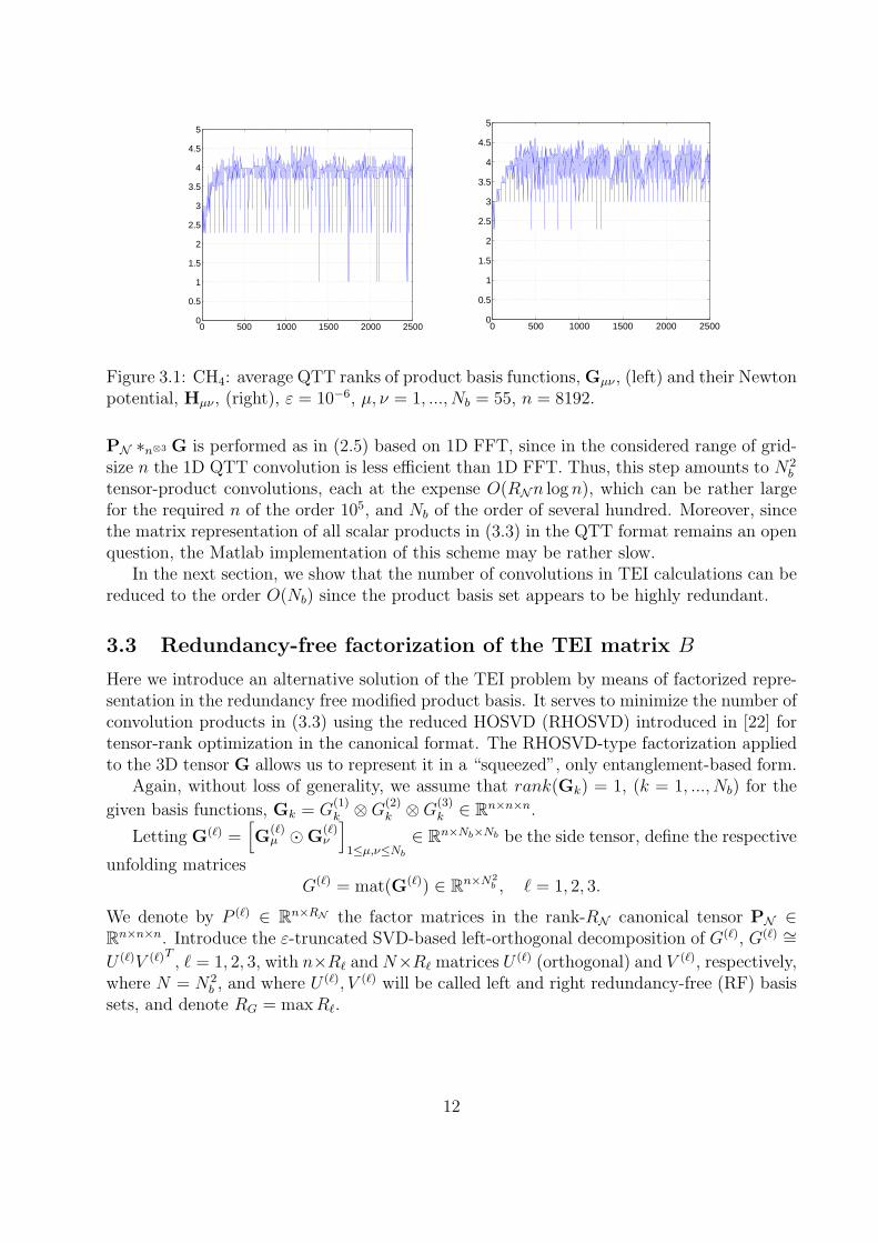
tensors. Now the result follows.Figure 3.1 illustrates the QTT-rank distribution for the precomputed canonical tensors
Gµν and Hµν (CH4 molecule) with grid-size n = 8192, Nb = 55, and N = 552 (cf. Lemmata3.4 and 3.5). One observes the uniform bound on QTT-rank for any combination of µ, ν.We also found the almost constant behavior of the QTT ranks along all virtual dimensionsin quantized representation of the respective n-vectors.
Now we summarize the complexity issues in computation the Newton potential of theproduct basis, Hµν , under assumption rank(Gµν) = 1.
Remark 3.6 For a fixed accuracy ε > 0, the set of tensors Hµν (µ, ν = 1, ..., Nb) can beprecomputed in the canonical tensor format at the expense O(RNN
2b n log n). Tensors Gµν
and Hµν can be stored in C-QTT format by O(N2b | log ε| log n) and O(N2
b | log ε|2 log2 n) reals,
respectively.
Proof. Follows by (3.4) and Lemmas 3.4 and 3.5.Given tensors G and H in the canonical-QTT format, each entry in TEI tensor B can
be calculated with O(log n) complexity. However, tensor-structured convolution step H =
11
0 500 1000 1500 2000 25000
0.5
1
1.5
2
2.5
3
3.5
4
4.5
5
0 500 1000 1500 2000 25000
0.5
1
1.5
2
2.5
3
3.5
4
4.5
5
Figure 3.1: CH4: average QTT ranks of product basis functions, Gµν , (left) and their Newtonpotential, Hµν , (right), ε = 10−6, µ, ν = 1, ..., Nb = 55, n = 8192.
PN ∗n⊗3 G is performed as in (2.5) based on 1D FFT, since in the considered range of grid-size n the 1D QTT convolution is less efficient than 1D FFT. Thus, this step amounts to N2
b
tensor-product convolutions, each at the expense O(RNn log n), which can be rather largefor the required n of the order 105, and Nb of the order of several hundred. Moreover, sincethe matrix representation of all scalar products in (3.3) in the QTT format remains an openquestion, the Matlab implementation of this scheme may be rather slow.
In the next section, we show that the number of convolutions in TEI calculations can bereduced to the order O(Nb) since the product basis set appears to be highly redundant.
3.3 Redundancy-free factorization of the TEI matrix B
Here we introduce an alternative solution of the TEI problem by means of factorized repre-sentation in the redundancy free modified product basis. It serves to minimize the number ofconvolution products in (3.3) using the reduced HOSVD (RHOSVD) introduced in [22] fortensor-rank optimization in the canonical format. The RHOSVD-type factorization appliedto the 3D tensor G allows us to represent it in a “squeezed”, only entanglement-based form.
Again, without loss of generality, we assume that rank(Gk) = 1, (k = 1, ..., Nb) for the
given basis functions, Gk = G(1)k ⊗G
(2)k ⊗G
(3)k ∈ Rn×n×n.
Letting G(`) =[G
(`)µ G
(`)ν
]1≤µ,ν≤Nb
∈ Rn×Nb×Nb be the side tensor, define the respective
unfolding matricesG(`) = mat(G(`)) ∈ Rn×N2
b , ` = 1, 2, 3.
We denote by P (`) ∈ Rn×RN the factor matrices in the rank-RN canonical tensor PN ∈Rn×n×n. Introduce the ε-truncated SVD-based left-orthogonal decomposition of G(`), G(`) ∼=U (`)V (`)T , ` = 1, 2, 3, with n×R` andN×R` matrices U (`) (orthogonal) and V (`), respectively,where N = N2
b , and where U (`), V (`) will be called left and right redundancy-free (RF) basissets, and denote RG = maxR`.
12

Lemma 3.7 Given ε > 0, the redundancy-free factorized ε-approximation to the matrix B,
B ∼= Bε :=
RN∑k=1
3`=1V
(`)M(`)k V (`)T , (3.5)
where V (`) is the corresponding right RF basis and
M(`)k = U (`)T (P
(`)k ∗n U (`)) ∈ RR`×R` , k = 1, ..., RN , (3.6)
stands for the Galerkin convolution matrix on the left RF basis, U (`), ` = 1, 2, 3, exhibits thefollowing properties:
(A) The storage demand for factorizations (3.5) and (3.6) is estimated by RN∑3
`=1R2` +
N2b
∑3`=1R` and O((RG +RN )n), respectively. The numerical complexity of the ε-truncated
representation (3.6) is bounded by O(RNR2Gn+RGRNn log n).
(B) The ε-rank of the matrix Bε admits the following upper bound,
rank(Bε) ≤ minN2b , RN
3∏`=1
R`. (3.7)
(C) Let A`(k) = G(`)P(`)k ∗n G(`), then the error estimate in the Frobenius norm holds,
‖B −Bε‖F ≤ 6εmax`
‖ G(`) ‖FRN∑k=1
max`
‖A`(k)‖2F ‖ P (`)k ‖F . (3.8)
(D) Assume that QTT ranks of the column vectors in P(`)k ∗nU (`) and U (`) are small. Then
the QTT representation of tensor factors in (3.6) amounts to O(RGRN log n) reals. The
QTT-complexity to compute matrices M(`)k , k = 1, ..., RN , is estimated by O(RNR
2G log n).
Proof. (A) Using the Galerkin-type representation of the TEI tensor B as in (3.3), we obtain
B = mat(B) =
RN∑k=1
3`=1G
(`)T[P
(`)k ∗n G(`)
],
where denotes the Hadamard product of matrices. Plugging the truncated SVD factor-ization of G(`) in the right-hand side above leads to the desired representation,
Bε =
RN∑k=1
3`=1V
(`)U (`)T[P
(`)k ∗n (U (`)V (`)T )
](3.9)
=
RN∑k=1
3`=1V
(`)[U `)T (P
(`)k ∗n U (`))
]V (`)T
=
RN∑k=1
3`=1V
(`)M(`)k V (`)T .
13

The storage cost for the above RHOSVD-type factorization (3.9) to the N2b ×N2
b matrix Bis bounded by RN
∑3`=1R
2` +N2
b
∑3`=1R` being independent on the grid-size n.
The computational complexity at this step is dominated by the cost of reduced Choleskyalgorithm to compute truncated SVD of matrices G(`), that is O(RG(N
2b + n)), and by the
total cost of convolution products in (3.6), O(RNRGn log n).(B) Using the rank properties of Hadamard product of matrices, it is easy to see that (3.9)
implies the direct ε-rank estimate for the matrix Bε, as in (3.7), where the rank parametersR` characterize the entanglement of a molecule.
(C) The error bound can be derived along the line of [22], Theorem 2.5 (d), related tothe RHOSVD error analysis. In fact, the approximation error can be represented by
B −Bε =
RN∑k=1
(3
`=1G(`)P
(`)k ∗n G(`) −3
`=1V(`)U (`)TP
(`)k ∗n U (`)V (`)T
).
Denote A`(k) = V (`)U (`)TP(`)k ∗n U (`)V (`)T , then for each fixed k = 1, . . . RN , we have
‖A` − A`‖ ≤ 2ε‖P (`)k ‖‖G(`)‖ (3.10)
since the stability in the Frobenius norm ‖U (`)V (`)T‖ ≤ ‖G(`)‖ holds. Now, for fixed k, weobtain
A1 A2 A3 − A1 A2 A3 = A1 A2 A3 − A1 A2 A3
+ A1 A2 A3 − A1 A2 A3
+ A1 A2 A3 − A1 A2 A3.
Summing up the above representation over k = 1, . . . RN , and taking into account (3.10), wearrive at the bound
‖B −Bε‖F ≤ 6εmax`
‖G(`)‖FRN∑k=1
max`
‖A`(k)‖2F‖P(`)k ‖F , (3.11)
which proves the result.(D) The complexity bound is the direct consequence of assumptions on the QTT-ranks
(see numerics below).Proof of Lemma 3.7 is constructive and outlines the way to an efficient implementation of
(3.5), (3.6). Some numerical results on performance of the corresponding black-box algorithmare shown in Sections 3.4 and 4.2. Here the algebraically optimized separation ranks R` areonly determined by the entanglement properties of a molecule, while the number N − RG
indicates the measure of redundancy in the product basis set. In numerical experiments weobserve R` ≤ Nb and R` n for large n.
Figure 3.2, left, represents the ε-rank R`, ` = 1, 2, 3, and RB, computed on the examplesof some compact molecules with ε = 10−6. We observe that the Cholesky rank of B, RB, isa multiple of Nb with a factor ∼ 6, see also Fig. 3.3. Remarkably, the RHOSVD separationranks R` ≤ Nb remain to be very weakly dependent on Nb, but primarily depend on thetopology of a molecule.
14

Molecules NH3 H2O2 N2H4 C2H5OH
Nb;Norb 48; 5 68; 9 82; 9 123; 13
Av. QTT rank of U (1) 7.3 7.9 7.5 7.6
Av. QTT rank of V (1) 15 21 24 37
(Av. QTT rank of V (1))/Norb 3 2.3 2.6 2.85
Table 3.1: Average QTT ε-ranks of U (1) and V (1) in G(1)-factorization, ε = 10−6.
Figure 3.2, right, provides average QTT ranks of column-vectors in U (1) ∈ Rn×R1 forNH3, H2O2, N2H4 and C2H5OH molecules. Again, surprisingly, the rank portraits appear tobe nearly the same for different molecules, and the average rank over all indices m = 1, ..., R1
is a small constant at about r0 w 7. The more detailed results are listed in Table 3.1.
40 50 60 70 80 90 100 110 1200
100
200
300
400
500
600
700
800
Nb
R1
R2
R3
RB
10 20 30 40 50 60 70 80 904
5
6
7
8
9
10
vectors of U(1)
Ave
rag
e Q
TT
ran
ks
Figure 3.2: Left: ε-ranks R` and RB for HF, NH3, H2O2, N2H4 and C2H5OH molecules, with thenumber of basis functions Nb = 34, 48, 68, 82 and 123, respectively. Right: Average QTT ε-ranksof column-vectors in U (1) ∈ Rn×R` for NH3, H2O2, N2H4 and C2H5OH molecules, ε = 10−6.
The a priori rank estimate (3.7) looks too pessimistic compared with the results of nu-merical experiments. However, in the case of flattened or extended molecules (some of thedirectional ranks are small) this estimate provides a much sharper bound.
The RHOSVD factorization (3.5), (3.6) is a reminiscent of the exact Galerkin represen-
tation (3.3) in the right RF basis, while matricesM(`)k play the role of ”directional“ Galerkin
projections of the Newton kernel onto the left RF basis. This factorization can be applied di-rectly to fast calculation of the reduced Cholesky decomposition of the matrix B consideredin the next section.
Finally, we point out that our RHOSVD-type factorization can be viewed as the algebraictensor-structured counterpart of the density fitting scheme commonly used in quantum chem-istry [1]. The robust error control in the proposed basis optimization approach is based onpurely algebraic SVD-like procedure that allows to eliminate the redundancy in the productbasis set up to given precision ε > 0.
15

3.4 Low-rank Cholesky decomposition of the TEI matrix B
In this section, we present the economical truncated Cholesky decomposition scheme ofcomplexity O(N3
b ) providing the O(Nb)-rank factorization of the TEI matrix B. Then wedescribe how the complexity can be reduced to O(N2
orbNb) using the quantized representa-tion of the Cholesky vectors. The Cholesky scheme requires only O(Nb) adaptively chosencolumns in B calculated on-line using the off-line precomputed data either in the form ofone-electron integral tensor H, or the redundancy-free factorization (3.5).
We denote the long indexes in the N ×N (N = N2b ) matrix unfolding B by
i = vec(µ, ν) := (µ− 1)Nb + ν, j = vec(κ, λ), i, j ∈ IN := 1, ..., N.
Lemma 3.8 The unfolding matrix B is symmetric and positive semidefinite.
Proof. The symmetry is enforced by the definition (see Lemma 3.2). The positive semi-definiteness follows from the observation that the matrix B can be viewed as the Galerkinmatrix 〈−∆−1ui, uj〉, i, j ∈ IN , in the finite product basis set ui = gµgν, where ∆−1 isthe inverse of the self-adjoint and positive definite in H1(R3) Laplacian operator subject tothe homogeneous Dirichlet boundary conditions at x→ ∞.
We consider the ε-truncated Cholesky factorization of B ≈ Bε = LLT , where
‖B − LLT‖ ≤ Cε, L ∈ RN×RB .
Based on the previous observation (see Introduction), we will postulate rather general ε-rankestimate (in electronic structure calculations this conventional fact traces back to [5]), seenumerics on Fig. 3.3.
Conjecture 3.9 Fixed truncation error ε > 0, for the Gaussian-type AO basis functionsthere holds, RB = rank(LLT ) ≤ CNb, where the constant C > 0 is independent of Nb.
Clearly, the fastest version of the numerical Cholesky decomposition is possible in thecase of given full TEI tensor B. In this case the CPU time for the Cholesky decomposi-tion becomes negligible compared with those to compute the TEI tensor B. However, thepractical use of algorithm is limited to the small basis sets because of the large storagerequirements, N4
b .In what follows, we describe the two approaches to compute the truncated Cholesky
decomposition with reduced storage demands based on different types of precomputed input:(A) one-electron integrals tensor H (see §3.1) or(B) the redundancy-free factorization of B in form (3.5).In case (A), we propose the optimized two-step approximation method to compute the
ε-truncated Cholesky factorization that operates on the input of the ”one-electron“ tensorsGµν and Hµν , both represented in the mixed canonical-QTT data format.
The complexity optimization is based on the idea to recognize the finer data structure byquantization of long n-vectors in precomputing stage using merely the algebraic algorithmswith controlled approximation error via the adaptive choice of separation rank parameters.
Suppose that n = 2L, then the rank-1 canonical tensorGµν = G(1)⊗G(2)⊗G(3) ∈ Rn×n×n,with G(`) ∈ Rn, is mapped to its quantized image in dimension D,
Gµν 7→ Q(Gµν) = Q(G(1))⊗Q(G(2))⊗Q(G(3)) ∈D⊗
ν=1
R2,
16

0 100 200 300 400 500 60010
−7
10−6
10−5
10−4
10−3
10−2
10−1
100
NH3
H2O
2
N2H
4
C2H
5OH
Figure 3.3: Singular values of LLT for NH3, H2O2, N2H4 and C2H5OH molecules, with thenumber Nb of basis functions 48, 68, 82 and 123, respectively.
with D = 3L and maximal QTT-rank rQ (for GTO basis we have rQ ≤ 4). Similar quanti-zation transform applies to each rank-1 term representing rank-RN tensor Hµν .
Quantization of the column N -vectors in the Cholesky factor L applies to their zeroextension to the size NQ = 2M ≥ N , that is nearest close to N = N2
b .
Algorithm (A). Given tensors Gµν and Hµν (µ, ν ∈ 1, ..., Nb) stored in the canonical-QTT format. Compute the optimized ε-truncated Cholesky decomposition in two steps:
(A.I) The Cholesky factorization calculates RB = O(Nb) required column vectors of sizeO(N), to be marked by indices j∗ = vec(κ∗, λ∗), by using scalar products in the QTT-canonical format
bµνκ∗λ∗ = 〈Gµν ,Hκ∗λ∗〉 ∈ RN .
Numerical cost for each N -vector amounts to 3 · 2r3Q log2 nN2b operations.
(A.II) Apply the rank-RL QTT approximation of dimension M ≈ log2N to the columnvectors (skeletons) of Cholesky factorization generating the mixed canonical-QTT tensordecomposition of the matrix B.
Fixed ε > 0, our numerical tests indicate the following asymptotic behavior (see Table3.3),
RL w 3Norb ≤3
10Nb,
that is to be postulated in the following. Hence, the total numerical cost to represent theLLT Cholesky decomposition is estimated by O(NbN
2orb log2Nb).
Table 3.2 provides the CPU times to calculate the convolution tensor H and then fullTEI tensor B on the example of the NH3 molecule (Nb = 48), ε = 10−6. It can be seen thatin the case of small molecules the precomputing step dominates over the direct evaluationof full tensor B and may quickly become a bottleneck for larger compounds. The CPU-timefor ε-Cholesky decomposition is about 1 sec., ε = 10−5.
17

n3 20483 40963 81923 163843
3D-Conv, H (sec) 8 41 112 182B (sec) 16 19 23 28
Table 3.2: NH3 molecule: CPU times for H and B vs. grid-size n3.
Case (B). In the situation with the precomputed RHOSVD-type factorization (3.5) onecan compute the truncated Cholesky decomposition using the column and diagonal elementsof matrix B calculated on the fly as in the following
Algorithm (B). Given the redundancy-free factorization (3.5).(B.I) Implement the Cholesky factorization where the column and diagonal elements in
the TEI matrix B are represented by the following tensor operations
B(:, j∗) =
RN∑k=1
3`=1V
(`)M(`)k V (`)(:, j∗)
T,
and
B(i, i) =
RN∑k=1
3`=1V
(`)(i, :)M(`)k V (`)(:, i)
T,
respectively.(B.II) Repeat Step (A.II) in Algorithm (A).The factorization (3.5) applied at Step (B.I) essentially reduces the amount of work on
the ”preprocessing“ stage in the limit of large Nb (see Lemma 3.7) since the number ofconvolutions is now estimated by CNb (usually, C ≤ 1) instead of N2
b .The cost to compute the column vector at Step (BI) is estimated by 3N2
bRG. Taking intoaccount that rQ ≈ 4 and RG ≤ Nb we conclude that in the range of grid-size n ≤ 214, Step(A.I) in Algorithm (A) outperforms Algorithm (B) if 2 · log2 n · r3Q = 2 · 14 · 43 ≤ Nb, i.e. forlarge enough Nb & 2000. The total numerical complexity of Step (BI) in Algorithm (B) isdominated by O(RGN
3b ).
3.5 Analyzing QTT compression to the Cholesky factor L
This section collects the important observations obtained in numerical experiments. In theQTT analysis of the TEI matrix B for several moderate size compact molecules, we revealedthat, with fixed approximation error ε > 0, the average QTT ranks of the Cholesky vectorshave the following behavior rQTT ∼ kcholNorb, with kchol ≤ 3. From this numerics we makea conclusion that factor kchol = 3 is due to the spatial dimensionality of the consideredmolecular system (or problem) observed for compact compounds and it becomes closer to 2for more stretched molecules, see Table 3.3 below.
Based on this numerical experiments we formulate our hypothesize:
Hypothesize 3.10 The structural complexity of the Cholesky factor L of matrix B in theQTT representation is characterized by the rank parameter
RL∼= 3Norb.
18

Molecule HF H2O NH3 H2O2 N2H4 C2H5OH
Norb 5 5 5 9 9 13rQTT 12 13.6 15 21 24 37
kchol = rQTT/Norb 2.4 2.7 3 2.3 2.6 2.85
Table 3.3: Average QTT ranks of the Cholesky vectors vs. Norb for some molecules.
The effective representation complexity of the Cholesky factor L ∈ RN×RB is estimated by
9RBN2orb RBN
2b .
Assuming that the conventional relation Nb ≈ 10Norb is fulfilled, we conclude that thereduction factor in the storage size with QTT representation of L is about 10−1.
Similar rank characterizations have been observed by the QTT analysis of U (`) and V (`)
factors in the rank factorization of the initial product bases tensors G(`), ` = 1, 2, 3 (seeTable 3.1).
It is interesting to note, that the average QTT ranks of the reduced higher order SVDfactors V (`) ∈ RN2
b×R` in the rank factorization of the initial product bases tensors G(`),` = 1, 2, 3, have almost the same rank scaling, rQ(V
(`)) ≤ 3Norb, as a factor kchol ≈ 3 in theCholesky decomposition of the matrix B (see Table 3.1). Hence, the QTT representationcomplexity for the factor V (`) in (3.5) can be reduced to
10N2orbRG ≈ 1
10N2
bRG.
4 Applications to electronic structure calculations
4.1 TEI tensor in the Hartree-Fock calculations
The numerical treatment of the two-electron integrals (TEI) is the main bottleneck in the fastsolution of the Hartree-Fock equation and in DFT calculations for large molecules. The 2N -electrons Hartree-Fock equation for pairwise L2-orthogonal electronic orbitals, ψi : R3 → R,ψi ∈ H1(R3), reads as
Fψi(x) = λi ψi(x),
∫R3
ψiψjdx = δij, i, j = 1, ..., Norb (4.1)
with F being the nonlinear Fock operator
F := −1
2∆ + Vc + VH +K.
Here the nuclear potential takes the form
Vc(x) = −M∑ν=1
Zν
‖x− aν‖, Zν > 0, aν ∈ R3,
19

while the Hartree potential VH(x) and the nonlocal exchange operator K read as
VH(x) := ρ ?1
‖ · ‖=
∫R3
ρ(y)
‖x− y‖dy, x ∈ R3, (4.2)
and
(Kψ) (x) := −Norb∑i=1
(ψ ψi ?
1
‖ · ‖
)ψi(x) = −1
2
∫R3
τ(x, y)
‖x− y‖ψ(y)dy, (4.3)
respectively. Conventionally, we use the definitions
τ(x, y) := 2
Norb∑i=1
ψi(x)ψi(y), ρ(x) := τ(x, x),
for the density matrix τ(x, y), and electron density ρ(x).Usually, the Hartree-Fock equation is approximated by the standard Galerkin projec-
tion of the initial problem (4.1) posed in H1(R3) (see [29] for more details). For a givenfinite Galerkin basis set gµ1≤µ≤Nb
, gµ ∈ H1(R3), the occupied molecular orbitals ψi arerepresented (approximately) as
ψi =
Nb∑µ=1
Cµigµ, i = 1, ..., Norb. (4.4)
To derive an equation for the unknown coefficients matrix C = Cµi ∈ RNb×Norb , first, weintroduce the mass (overlap) matrix S = Sµν1≤µ,ν≤Nb
, given by
Sµν =
∫R3
gµgνdx,
and the stiffness matrix H = hµν of the core Hamiltonian H = −12∆ + Vc (the single-
electron integrals),
hµν =1
2
∫R3
∇gµ · ∇gνdx+∫R3
Vc(x)gµgνdx, 1 ≤ µ, ν ≤ Nb.
The core Hamiltonian matrix H can be precomputed in O(N2b ) operations, see [21] for the
detailed description of the grid-based approach.In computational quantum chemistry the nonlinear terms representing the Galerkin ap-
proximation to the Hartree and exchange operators are calculated traditionally by using thetwo-electron integrals tensor B = [bµνκλ] as defined in (1.1), that initially has the computa-tional and storage complexity of order O(N4
b ).Introducing the Nb ×Nb matrices J(D) and K(D),
J(D)µν =
Nb∑κ,λ=1
bµν,κλDκλ, K(D)µν = −1
2
Nb∑κ,λ=1
bµλ,νκDκλ, (4.5)
where D = 2CCT ∈ RNb×Nb is the low-rank symmetric density matrix, such that
rank(D) = Norb Nb,
20

one then represents the complete Fock matrix F by
F (D) = H + J(D) +K(D). (4.6)
The resultant Galerkin system of nonlinear equations for the coefficients matrixC ∈ RNb×Norb , and the respective eigenvalues Λ, reads as
F (D)C = SCΛ, Λ = diag(λ1, ..., λNb), (4.7)
CTSC = IN ,
where the second equation represents the orthogonality constraints∫R3 ψiψjdx = δij. Here
IN denotes the Nb ×Nb identity matrix.In the standard quantum chemical implementations based on the analytically precom-
puted set of two-electron 3D convolution integrals, the numerically confirmed rank boundrank(B) ≤ CBNb (CB ∼ 10), allows to reduce the complexity of building up the Fock matrixF to O(N3
b ), which is by far dominated by computational cost for the exchange term K(D).In the following we will show how this cost can be reduced further using certain low-rankstructures in matrices B and D.
4.2 The Hartree-Fock calculus using tensor structure in B
In this Section we consider in more detail the multilinear algebraic calculation of the Coulomband exchange matrices in the Fock operator. One can use the canonical-QTT structure ofthe target tensor and low-rank structure of the matrix D to evaluate and represent matricesJ(D) and K(D) efficiently.
Remark 4.1 (The Coulomb matrix). Precomputed tensors Gµν ,Hκλ, in view of (3.1), wehave
J(D)µν =
Nb∑κ,λ=1
bµν,κλDκλ =
Nb∑κ,λ=1
〈Gµν ,Hκλ〉Dκλ. (4.8)
Vectorizing matrices J = vec(J), D = vec(D), we arrive at the simple matrix representation,
J = BD ≈ L(LTD), (4.9)
which can be easily evaluated taking into account the rank structure of B as well as theQTT-structure in vectors D and in the column vectors of L.
The straightforward calculation by (4.9) amounts to O(RBN2b ) operations where RB is the
ε-rank of B. Our analysis indicates that imposing the QTT-structure of the matrix L mayreduce this cost to O(RBNorb).
Remark 4.2 (The HF exchange). Tensor evaluation of the exchange matrix K(D) is muchmore involved since in this case it reduces to a summation over permuted indices,
K(D)µν = −1
2
Nb∑κ,λ=1
bµλ,νκDκλ = −1
2
Nb∑κ,λ=1
〈Gµλ,Hνκ〉Dκλ. (4.10)
21

Figure 4.1: N2H4 molecule: error in the Coulomb (left) and exchange (right) matrices, usingthe Richardson extrapolation on n⊗3 grids with n = 8192 and n = 16384.
2040
6080
100120
2040
6080
100120
0
1
2
3
4x 10
−3
2040
6080
100120
2040
6080
100120
0
0.2
0.4
0.6
0.8
1
x 10−3
Figure 4.2: C2H5OH molecule: accuracy of the exchange matrices on n⊗3 grids with n = 8192and n = 16384 (the decay ratio 1 : 4 is well suited for the Richardson extrapolation).
22

Introducing the permuted tensor B = permute(B, [2, 3, 1, 4]), and the respective accompany-
ing matrix B = mat(B), we then obtain
vec(K) = K = BD. (4.11)
The calculation by (4.11) amounts to O(RBN3b ) operations. However, using the rank-Norb
decomposition of D = 2CCT allows to reduce the cost to O(RBNorbN2b ), by the representation,
K(D)µν = −Norb∑i=1
(∑
LµλCλi)(∑
LκνCκi)T ,
where Lµν = reshape(L, [Nb, Nb, RB]) ∈ RNb×Nb×RB is the Nb × Nb × RB-folding of theCholesky factor L.
In this work the numerical illustrations are performed using the grid representation of Gaus-sian AO bases merely to have means to compare the accuracy of the resulting Galerkin Fockmatrix with a standard output from the MOLPRO package [40], where the entries of TEIsare computed analytically.
Figure 4.1 represents the error portrait corresponding to the Coulomb and exchangematrices computed via rank-RB LLT approximation to B as above, in the case of N2N4
molecule. Figure 4.2 shows the absolute error in the exchange matrix of C2H5OH moleculecalculated on n⊗3 grids with n = 8192 and n = 16384. The numerical error scales quadrati-cally in the grid size, O(h2), and can be improved to O(h3) by the Richardson extrapolation.The observed decay ratio 1 : 4 indicates the applicability of Richardson extrapolation to theresults on a pair of diadically refined grids.
4.3 MP2 perturbation theory
The various degrees Møller-Plesset perturbation theory (in particular, second-order MP2model) significantly improves the HF correlation energy and other molecular characteriza-tions in the case of large basis sets [41]. However, the numerical payoff scales as N5
b . Ourtensor-structured representations of the matrix B allows to reduce this cost by some ordersof magnitude. Here we sketch the main idea.
First, one has to transform the TEI tensor B = [bµνκλ], from the initial AO basis set tothe MO-basis represented by (4.4),
V = [viajb] : viajb =
Nb∑µ,ν,λ,σ=1
CµiCνaCλjCσbbµνλσ, i, a, j, b ∈ 1, ..., Nb,
that makes the dominating impact to the overall numerical cost of order O(N5b ). Given the
tensor V = [viajb], then the second order MP2 perturbation to the HF energy is calculatedby
EMP2 = −∑
a,b∈Ivir
∑i,j∈Iocc
viajb(2viajb − vibja)
εa + εb − εi − εj,
where Iocc := 1, ..., Norb, Ivir := Norb + 1, ..., Nb, and εk, k = 1, ..., Nb, represent the HFeigenvalues.
23

It can be shown that the rank-O(Nb) approximation to the TEI matrix B and to thematrix unfolding of V, V = [via;jb], combined with the low-rank approximation to theunfolding matrix E of a tensor
E = [1
εa + εb − εi − εj], i, a, j, b ∈ 1, ..., Nb, (4.12)
reduces the total cost by the order of magnitude (we suppose that the so-called homo-lumogap is larger than some fixed constant δ > 0). In this aspect, the rank-| log ε log δ| approx-imation to the unfolding matrix E = [ek`,mn] follows by the well-known sinc-approximationto the Hilbert matrix 1
i+j, [12].
Further reduction of the numerical complexity can be based on more specific propertiesof the matrix unfolding V when using a physical insight to the problem.
4.4 Multidimensional Hamiltonian in FCI models
In the formulation of second quantization, the Hamiltonian operator for the high-dimensionalelectronic Schrodinger equation
HΨ = EΨ
is given by
H =∑pq
hpqa+q ap +
1
2
∑pq,rs
vqspra+r a
+s a
−p a
−q ,
where the single-electron integrals correspond to the core Hamiltonian in HF operator (see§4.1), and vqspr represents the TEI in the MO basis (the so-called canonical molecular or-bitals). The symbols a+ and a− denote creation and annihilation operators of second quan-tization. The details on electronic structure calculations via FCI models, particularly basedon DMRG optimization over MPS-type tensor manifolds, can be found in the seminal paper[42].
5 Conclusions
In this paper, we present a new grid-based tensor-structured method for the efficient cal-culation of the TEI tensor in a general low-rank basis. The approach is based on thetensor-product numerical integration, redundancy-free matrix factorizations on the opti-mized product-basis, and, finally, the pivoted Cholesky decomposition of the TEI matrix Baccomplished by the QTT-recompression of the column vectors in the Cholesky factor.
Due to the O(n log n) complexity scaling of the tensor-structured numerical convolutionover n× n× n Cartesian grids, and, hence, the possibility to imply fine spatial meshes, weachieve high accuracy in the Coulomb and exchange matrices on examples of several organicmolecules. The computational error is of the order O(h2), where h is the mesh-size, and itcan be reduced to O(h3) by using the Richardson extrapolation. Making use of the quantizedrepresentation to grid functions allows to reduce the storage complexity to the logarithmicscaling in n, O(log n).
The main theoretical results of the paper are concerned with the QTT rank boundsproven for the GTO basis tensor G and for its Newtonian convolution H, see Lemmas 3.4
24

and 3.5, and summarized in Remark 3.6 in the form of rigorous complexity bounds. Theseresults justify the logarithmic complexity scaling in the mesh parameter n of the importantprecomputing step as in §3.2. We also prove the complexity and error estimates for theredundancy-free factorization of the TEI matrix, presented in Lemma 3.3.
We revealed in numerical tests that the separation ranks of the redundancy-free factor-ization to the matrix B remain to be bounded by Nb, while the ε-rank of the TEI matrix Bitself has clear linear scaling in Nb. The structural complexity of the quantized representa-tion to the Cholesky vectors, measured by the QTT-ranks, is close to 3Norb. The importantnumerical observation in the paper is that the storage complexity of Cholesky decomposi-tion scales as O(32N2
orbNb), reducing at about a factor of 10−1 the traditional scaling O(N3b ),
since, conventionally, Nb w 10Norb.The presented method has a good potential for the post-HF models, since the higher
dimensionality of tensor data makes the effect of multilinear algebra even more essential.
Acknowledgements. The authors are grateful Dr. habil. Dirk Andre (FU Berlin) andto Dr. Heinz-Juergen Flad (TU Munich) for valuable discussions. We are thankful to Dr.D. Savostianov (Uni. Southampton, UK) for the assistance with implementation of theincomplete Cholesky decomposition.
References
[1] J. Almlof. Direct methods in electronic structure theory. In D. R. Yarkony: Modern Electronic StructureTheory. vol II, World Scientific, Singapore, 1995 pp. 110-151.
[2] P. Y. Ayala and G. E. Scuseria. Linear scaling second-order Møller-Plesset theory in the atomic orbitalbasis for large molecular systems. J. Chem. Phys. v. 110 No. 8, 1999, pp.3660-3671.
[3] M. Barrault, E. Cances, W. Hager and C. Le Bris. Multilevel domain decomposition for electronicstructure calculations. J. Comput. Phys. 222, 2007, 86-109.
[4] M. Bebendorf and S. Rjasanow. Adaptive low-rank approximation of collocation matrices. Computing,70(1):1-24, 2003.
[5] N.H.F. Beebe and J. Linderberg. Simplifications in the generation and transformation of two-electronintegrals in molecular calculations. Int. Quantum Chem., v 12 7:683-705, 1977.
[6] C. Bertoglio, and B.N. Khoromskij. Low-rank quadrature-based tensor approximation of the Galerkinprojected Newton/Yukawa kernels. Comp. Phys. Communications, v. 183(4), 904-912 (2012).
[7] I.P. Gavrilyuk, W. Hackbusch, and B.N. Khoromskij. Tensor-product approximation to elliptic andparabolic solution operators in higher dimensions. Computing 74 (2005), 131-157.
[8] S. A. Goreinov, E. E. Tyrtyshnikov and N. L. Zamarashkin. A theory of pseudoskeleton approximations.Linear Alebra Appl., 261, 1997, 1-21.
[9] S.V. Dolgov, B.N. Khoromskij, and I. Oseledets. Fast solution of multi-dimensional parabolic problemsin the TT/QTT formats with initial application to the Fokker-Planck equation. SIAM J. on Sci. Comp.,2012 (accepted). Preprint 80/2011, MPI MiS, Leipzig 2011.
[10] S.V. Dolgov, B.N. Khoromskij, and D. Savostianov. Superfast Fourier transform using QTT approxi-mation. J. Fourier Anal. Appl., 2012, vol.18, 5, 915-953.
[11] S.V. Dolgov, and B.N. Khoromskij. Two-level Tucker-TT-QTT format for optimized tensor calculus.Preprint 19/2012, MPI MiS, Leipzig 2012 (SIMAX, submitted).
25

[12] W. Hackbusch and B.N. Khoromskij. Low-rank Kronecker product approximation to multi-dimensionalnonlocal operators. Part I. Separable approximation of multi-variate functions; Computing 76 (2006),177-202.
[13] H. Harbrecht, M. Peters, and R. Schneider. On the low-rank approximation by the pivoted Choleskydecomposition. App. Numer. Math., 62(4), 2012, 428-440.
[14] R.J. Harrison, G.I. Fann, T. Yanai, Z. Gan, and G. Beylkin. Multiresolution quantum chemistry: Basictheory and initial applications. J. of Chemical Physics, 121 (23): 11587-11598, 2004.
[15] T. Helgaker, P. Jørgensen and J. Olsen. Molecular Electronic-Structure Theory. Wiley, New York, 1999.
[16] N. Higham. Analysis of the Cholesky decomposition of a semi-definite matrix. In M.G. Cox and S.J.Hammarling, eds. Reliable Numerical Computations, p. 161-185, Oxford University Press, Oxford, 1990.
[17] S. Holtz, T. Rohwedder, and R. Schneider. On manifolds of tensors of fixed TT-rank, Numer. Math.,120(12) pp.701-731, 2012.
[18] V. Kazeev, B.N. Khoromskij, and E.E. Tyrtyshnikov. Multilevel Toeplitz matrices generated by QTTvectors and convolution with logarithmic complexity. Preprint 36/2011, MPI MiS, Leipzig 2011, (SISC,submitted).
[19] V. Khoromskaia. Computation of the Hartree-Fock exchange by the tensor-structured methods. Comp.Meth. in Applied Math., Vol. 10 , No 2, 204-218, 2010.
[20] V. Khoromskaia, B.N. Khoromskij, and R. Schneider. QTT representation of the Hartree and exchangeoperators in electronic structure calculations. Comp. Meth. in Applied Math., v.11, No. 3, 327-341,2011.
[21] V. Khoromskaia, D. Andrae, and B.N. Khoromskij. Fast and accurate 3D tensor calculation of the Fockoperator in a general basis. Comp. Phys. Communications, 183 (2012) 2392-2404.
[22] B.N. Khoromskij and V. Khoromskaia. Multigrid tensor approximation of function related multidimen-sional arrays. SIAM J. on Sci. Comp., 31(4), 3002-3026, 2009.
[23] B.N. Khoromskij, V. Khoromskaia, and H.-J. Flad. Numerical solution of the Hartree-Fock equation inmultilevel tensor-structured format. SIAM J. on Sci. Comp., 33(1), 45-65, 2011.
[24] B.N. Khoromskij. O(d logN)-Quantics approximation of N -d tensors in high-dimensional numericalmodeling. J. Constr. Approx., v.34(2), 2011, 257-280.
[25] B.N. Khoromskij. Fast and accurate tensor approximation of a multivariate convolution with linearscaling in dimension. J. of Comp. Appl. Math., 234 (2010) 3122-3139.
[26] B.N. Khoromskij. Tensors-structured numerical methods in scientific computing: survey on recent ad-vances. Chemometrics and Intellingent Laboratory Systems, 110 (2012),1-19.
[27] T.G. Kolda and B.W. Bader. Tensor decompositions and applications. SIAM Review, 51/3, 2009 455-500.
[28] H. Luo, W. Hackbusch and H.-J. Flad. Quantum Monte Carlo study of Jastrow perturbation theory. I.Wavefunction optimization. J. Chem. Phys., 131, 104106, 2009.
[29] C. Le Bris, Computational chemistry from the perspective of numerical analysis. Acta Numerica (2005),363 - 444.
[30] I.V. Oseledets. Tensor-train decomposition. SIAM J. Sci. Comp., v. 33(5), 2295-2317 (2011).
[31] I.V. Oseledets, Approximation of 2d × 2d matrices using tensor decomposition. SIAM J. Matrix Anal.Appl., 31(4):2130-2145, 2010.
[32] I.V. Oseledets, and E.E. Tyrtyshnikov, Breaking the curse of dimensionality, or how to use SVD inmany dimensions. SIAM J. Sci. Comp., 31 (2009), 3744-3759.
[33] P. Pulay. Improved SCF convergence acceleration. J. Comput. Chem. 3, 556-560 (1982).
26

[34] G. Rauhut, P. Pulay, H.-J. Werner. Integral transformation with low-order scaling for large local second-order Mollet-Plesset calculations. J. Comp. Chem. 19, 1998, pp.1241-1254.
[35] D. V. Savostianov. Fast revealing of mode ranks of tensor in canonical form. Numer. Math. Theor.Meth. Appl. v.2 No.4 2009 pp439-444.
[36] N. D. Sidiropoulos. Generalized Carath‘eodory’s Uniqueness of harmonic Parametrization to N Dimen-sions. IEE Trans. Inform. Theory, 47 (2001) 1687-1690.
[37] E. E. Tyrtyshnikov. Mosaic-skeleton approximation. Calcolo, 33, 1996, 47-57.
[38] F. Verstraete, D. Porras, and J.I. Cirac, DMRG and periodic boundary conditions: A quantum infor-mation perspective. Phys. Rev. Lett., 93(22): 227205, Nov. 2004.
[39] G. Vidal. Efficient classical simulation of slightly entangled quantum computations. Phys. Rev. Lett.91(14), 2003, 147902-1 147902-4.
[40] H.-J. Werner, P.J. Knowles, et al. MOLPRO, Version 2002.10, A package of ab initio programs forelectronic structure calculations.
[41] H.-J. Werner, F.R. Manby, and P.J. Knowles. Fast linear scaling second order Møller-Plesset pertur-bation theory (MP2) using local and density fitting approximations. J. Chem. Phys., 118:8149-8160,2003.
[42] S.R. White. Density-matrix algorithms for quantum renormalization groups. Phys. Rev. B, v. 48(14),1993, 10345-10356.
[43] S. Wilson. Universal basis sets and Cholesky decomposition of the two-electron integral matrix. Comput.Phys. Commun., 58:71-81, 1990.
27