maximum recovery of mechanical energy through work
TRANSCRIPT

Wayne State University
Wayne State University Dissertations
1-1-2018
Maximum Recovery Of Mechanical EnergyThrough Work Integration: A Work ExchangeNetwork Synthesis ApproachAida Amini RankouhiWayne State University,
Follow this and additional works at: https://digitalcommons.wayne.edu/oa_dissertations
Part of the Chemical Engineering Commons
This Open Access Dissertation is brought to you for free and open access by DigitalCommons@WayneState. It has been accepted for inclusion inWayne State University Dissertations by an authorized administrator of DigitalCommons@WayneState.
Recommended CitationAmini Rankouhi, Aida, "Maximum Recovery Of Mechanical Energy Through Work Integration: A Work Exchange Network SynthesisApproach" (2018). Wayne State University Dissertations. 2005.https://digitalcommons.wayne.edu/oa_dissertations/2005

MAXIMUM RECOVERY OF MECHANICAL ENERGY THROUGH WORK
INTEGRATION: A WORK EXCHANGE NETWORK SYNTHESIS APPROACH
by
AIDA AMINI RANKOUHI
DISSERTATION
Submitted to the Graduate School
of Wayne State University,
Detroit, Michigan
in partial fulfillment of the requirements
for the degree of
DOCTOR OF PHILOSOPHY
2018
MAJOR: CHEMICAL ENGINEERING
Approved by:
____________________________________
Advisor Date
____________________________________
____________________________________
____________________________________
____________________________________

© COPYRIGHT BY
AIDA AMINI RANKOUHI
2018
All Rights Reserved

ii
DEDICATION
To Homeira, Masoud,
Anoosheh, and Pedram

iii
ACKNOWLEDGEMENTS
I would like to express my sincere appreciation to my advisor, Dr. Yinlun Huang, for his
continuous support and mentorship throughout my Ph.D. study at Wayne State University. His
guidance, encouragement, patience, and criticism helped me in growing as a researcher and
engineer. I could not have imagined having a better advisor and I believe the lessons I learned
from him would be the invaluable assets for my future career.
I am profoundly grateful to the members of my dissertation committee, Drs. Charles
Manke, Cristina Piluso, Evrim Dalkiran, and Helen E Durand for their insightful comments,
support, and encouragement. Additionally, I am very grateful for the support and friendship I was
offered by past and current lab members: Hao Song, Shaoqing Bai, Navdeep Bhadbhade, Majid
Moradi-Aliabadi, Raha Gerami, and Seyedparham Pourmirjafari-Firouzabadi.
I gratefully acknowledge the funding sources from National Science Foundation and
Graduate School of Wayne State University that made my Ph.D. work possible.
A special thanks to Dr. Guangzhao Mao, Dr. Korosh Torabi, Dr. Steven Salley, Angela
Childrey, Tracy Castle, my friends at ChE/MSE Graduate Students Organization, and Chloe Luyet.
I am extremely thankful to my industrial mentor, Dr. Sam Kharchenko, for his valuable guidance
and advice. Additionally, I greatly appreciate all the staff at Wayne State University who made the
school feels like home.
Finally, and most importantly, I would like to express gratitude to my parents, Homeira
Jamali and Masoud Amini-Rankouhi, for their endless love, support, sacrifices, and teaching me
to be independent, to work hard, to care for people and to live with honesty, my sister, Anoosheh
Amini-Rankouhi, for her selfless love and care, my husband, Pedram Jahanian, for his unfailing
love, encouragement, and understating during my pursuit of Ph.D. degree, and my best friends,
Neshat Basiri and Mohammad Soroush Barhaghi, for being there for me through the life’s thick

iv
and thin. I would also like to thank my aunt, Mehrshid, my uncle, Ali, my cousins, Babak and
Arezou, my friends back home, Shirin, Maryam, Matin, Sara, and Sepideh, and my dear friends in
Michigan, for the wonderful companionship during the past six years.

v
TABLE OF CONTENTS
DEDICATION ........................................................................................................................... ii
ACKNOWLEDGEMENTS ...................................................................................................... iii
LIST OF TABLES .................................................................................................................. viii
LIST OF FIGURES .................................................................................................................... x
CHAPTER 1 INTRODUCTION ............................................................................................... 1
1.1 Main Goals and Scientific Contributions ............................................................. 1
1.2 Organization of Dissertation ................................................................................ 3
CHAPTER 2 MECHANICAL ENERGY RECOVERY THROUGH WORK EXCHANGER
NETWORK INTEGRATION: CHALLENGES AND OPPORTUNITIES ....... 6
2.1 Mechanical Energy Recovery Fundamentals....................................................... 7
2.2 WEN Synthesis-Progress Overview .................................................................. 15
2.3 Challenges and Opportunities ............................................................................ 18
CHAPTER 3 PREDICTION OF MAXIMUM RECOVERABLE MECHANICAL ENERGY
VIA WORK INTEGRATION: A THERMODYNAMIC MODELING AND
ANALYSIS APPROACH ................................................................................. 22
3.1 Mathematical Framework for Energy Recovery Targeting ............................... 22
3.2 Case Studies ....................................................................................................... 32
3.2.1 Case 1- Prediction of the Maximum Recoverable Mechanical Energy of
a System Operated under Isothermal Conditions................................... 32
3.2.2 Case 2 – Prediction of the Maximum Recoverable Mechanical Energy of
a System Operated under Adiabatic Conditions .................................... 41
3.3.3 Discussion .............................................................................................. 48
3.4 Summary ............................................................................................................ 48
CHAPTER 4 SYNTHESIS OF COST EFFECTIVE HEAT INTEGRATED WORK
EXCHANGE NETWORK ................................................................................ 50
4.1 Work Exchanger Network Synthesis Methodology .......................................... 50
4.2 Heat Integrated Work Exchange Network Design ............................................. 57

vi
4.2.1 WEN Design Modification using Heat Integration ................................ 63
4.3 Basic Cost Analysis ........................................................................................... 64
4.4 Case Studies ....................................................................................................... 66
4.5 Summary ............................................................................................................ 95
CHAPTER 5 MODELING AND SIMULATION OF A PISTON-TYPE WORK
EXCHANGER FOR MECHANICAL ENERGY RECOVERY....................... 97
5.1 Objectives and Significance ............................................................................... 97
5.2 Modeling and Simulation of Work Exchanger Systems Using Aspen Plus .... 100
5.2.1 Construction of work exchanger module with Aspen Plus .................. 101
5.2.2 Simulation Procedures.......................................................................... 103
5.2.3 Simulation Results................................................................................ 105
5.3 CFD-based Modeling and Simulation of Piston-type Direct Work Exchanger109
5.3.1 Challenges and Opportunities .............................................................. 110
5.3.2 Piston-Type Work Exchanger Configuration ....................................... 113
5.3.3 Modeling Piston Dynamics .................................................................. 114
5.3.4 Simulation System Setup ..................................................................... 116
5.3.5 Analysis of Direct Piston-type Work Exchanger Full Cycle ............... 120
5.4 Summary .......................................................................................................... 131
CHAPTER 6 DATA-DRIVEN MODELING AND ANALYSIS OF ENERGY EFFICIENCY
OF GEOGRAPHICALLY DISTRIBUTED MANUFACTURING ............... 133
6.1 Data-driven Energy Analysis Methodology .................................................... 135
6.2 Case Study ....................................................................................................... 144
6.3 Summary .......................................................................................................... 162
CHAPTER 7 CONCLUSIONS AND FUTURE WORK ...................................................... 164
7.1 Conclusions ...................................................................................................... 164
7.2 Future Work ..................................................................................................... 167

vii
APPENDICES ........................................................................................................................ 172
Appendix A ............................................................................................................... 172
Appendix B ............................................................................................................... 177
Appendix C ............................................................................................................... 180
REFERENCES ....................................................................................................................... 189
ABSTRACT ......................................................................................................................... 197
AUTOBIOGRAPHICAL STATEMENT .............................................................................. 199

viii
LIST OF TABLES
Table 2.1. Evaluation of mechanical energy exchanged by process streams under different
operating conditions .................................................................................................... 11
Table 3.1. Process stream data for Case 1 ................................................................................... 34
Table 3.2. Energy recovery analysis for Case 1........................................................................... 40
Table 3.3. Performance comparison of WENs by different methods for Case 1......................... 41
Table 3.4. Process stream data for Case 2 ................................................................................... 43
Table 3.5. Energy recovery analysis for Case 2........................................................................... 45
Table 3.6. Performance comparison of WENs by different methods for Case 2......................... 46
Table 4.1. Directory of formulas to be used in prediction and synthesis stages for HEN located
before/after WEN design ............................................................................................ 62
Table 4.2. Process stream data for Case 1 ................................................................................... 67
Table 4.3. Energy recovery and operation cost comparison based on HEN location for Case 1 71
Table 4.4. Energy recovery analysis for Case 1........................................................................... 79
Table 4.5. Process stream data for Case 2 ................................................................................... 80
Table 4.6. Energy recovery and operation cost comparison based on HEN location for Case 2 83
Table 4.7. CAPEX and OPEX of units in Case 2 ........................................................................ 93
Table 4.8. Performance comparison of HIWENs by different methods for Case 2 .................... 94
Table 6.1. Manufacturing-sector-based energy consumption percentage in the U.S. in 2012 .. 148
Table 6.2. Manufacturing-sector-based energy loss percentage in the U.S. in 2012 ................. 149
Table 6.3. Manufacturing-sector-based energy consumption and total value of shipment in the
U.S. and State of MI in 2012 .................................................................................... 153
Table 6.4. Manufacturing-sector-based energy consumption in State of MI in 2012 ............... 154
Table 6.5. Manufacturing-sector-based energy loss percentage in MI in 2012 ......................... 156
Table 6.6. Manufacturing-sector-based energy loss in MI in 2012 ........................................... 157
Table 6.7. Total value of shipment for manufacturing sectors in three energy intensive counties
in MI.......................................................................................................................... 160

ix
Table 6.8. Manufacturing-sector-based energy consumption and direct loss in three energy
intensive counties in MI ............................................................................................ 161
Table 6.9. Carbon dioxide emission of MI and three counties with respect to manufacturing
sectors ....................................................................................................................... 161

x
LIST OF FIGURES
Figure 2.1. Sketch of work transfer units: (a) a (flow) WE and (b) an SSTC. ............................. 8
Figure 2.2. Valve position in each operational step of a work exchanger: (I) depressurization
step; (II) low-pressure displacement step; (III) pressurization step; (IV) high-
pressure displacement step. ........................................................................................ 9
Figure 2.3. P-V diagram for a flow work exchanger. ................................................................. 12
Figure 2.4. P-V-W diagram for work exchanger........................................................................ 13
Figure 2.5. P-W diagram for the work exchanger. ..................................................................... 14
Figure 2.6. Comparison of (a) heat transfer in a HE and (b) work transfer in a WE. ................ 19
Figure 3.1. Flowchart for derivation of matrix Γ . ................................................................... 25
Figure 3.2. Flowchart for evaluation of maximum recoverable mechanical energy. ................. 33
Figure 3.3. Work exchange networks designed by different methods for Case 1: (a) the solution
by the proposed model-based method to achieve the maximum energy recovery,
and (b) the solution derived by Liu et al. (2014). .................................................... 42
Figure 3.4. Flowsheet of heat-integrated work exchange network for Case 2: (a) work
exchanger network, and (b) heat exchanger network. ............................................. 47
Figure 4.1. Generation of WW and MP . .................................................................................. 56
Figure 4.2. Generation of 1C
W , 2C
W ,and EW . ........................................................................ 57
Figure 4.3. Flowchart for HEN location decision making. ........................................................ 59
Figure 4.4. (a) HEN located before WEN design, and (b) HEN located after WEN design. .... 60
Figure 4.5. Cost estimation for one work exchanger unit. ......................................................... 65
Figure 4.6. (a) HEN located before WEN design for Case 1, and (b) HEN located after WEN
design for Case 1. ..................................................................................................... 70
Figure 4.7. Flowsheet of heat-integrated work exchange network for Case 1 :(a) work
exchanger network, (b) heat exchanger network. .................................................... 78
Figure 4.8. Flowsheet of modified heat-integrated work exchange network for Case 1. .......... 79
Figure 4.9. (a) HEN located before WEN design for Case 2, and (b) HEN located after WEN
design for Case 2. ..................................................................................................... 84

xi
Figure 4.10. Flowsheet of heat-integrated work exchange network for Case 2: (a) work
exchanger network, and (b) heat exchanger network. ............................................. 92
Figure 5.1. Schematic illustration of a piston-type work exchanger (Cheng and Fan, 1968). ... 99
Figure 5.2. Schematic representation of a work exchanger module. ....................................... 101
Figure 5.3. Summary of the Excel model set up. ..................................................................... 105
Figure 5.4. Work exchanger unit in the Aspen Plus environment. .......................................... 106
Figure 5.5. Inlet data required to run the simulation. ............................................................... 107
Figure 5.6. Final streams and unit capacity results for Case 1. ................................................ 108
Figure 5.7. Simulated work exchanger network in Aspen Plus for Case 2. ............................. 109
Figure 5.8. Single piston hydraulic free-piston engine (Mikalsen and Roskilly, 2009). .......... 111
Figure 5.9. Piston-type work exchanger geometry model. ....................................................... 114
Figure 5.10. The balance of forces on the piston. ...................................................................... 115
Figure 5.11. An inlet check valve with one DOF translation (Ansys Inc. Fluent Theory Guide,
2017). ..................................................................................................................... 120
Figure 5.12. Contours of pressure variation during stages I-II. ................................................. 123
Figure 5.13. Contours of pressure variation during stages III-IV. ............................................. 124
Figure 5.14. Pressure change profile for HP and LP streams in full cycle (Stages I-IV). ......... 125
Figure 5.15. Piston position in a full cycle (Stages I-IV). .......................................................... 125
Figure 5.16. Valve no. 1 (inlet low-pressure stream) position during the full cycle (Stages I-IV).
................................................................................................................................ 126
Figure 5.17. Valve no. 2 (outlet low-pressure stream) position during the full cycle (Stages I-IV).
................................................................................................................................ 126
Figure 5.18. Valve no. 3 (inlet high-pressure stream) position during the full cycle (Stages I-IV).
................................................................................................................................ 127
Figure 5.19. Valve no. 4 (outlet high-pressure stream) position during the full cycle (stages I-
IV). ......................................................................................................................... 127
Figure 5.20. Piston position vs. time under different operating pressures. ................................ 129
Figure 5.21. Piston position vs. time under different operating temperatures. .......................... 130

xii
Figure 5.22. The compression ratio of the low-pressure stream for a maximum displacement of
the piston. ............................................................................................................... 131
Figure 6.1. Chemical sector manufacturing energy and carbon footprint (U.S. DOE, 2012). . 146
Figure 6.2. Manufacturing energy consumption map. ............................................................. 152
Figure 6.3. Manufacturing carbon dioxide emission map. ....................................................... 158
Figure 6.4. Manufacturing energy consumption in counties of Michigan. .............................. 160
Figure 6.5. Energy consumption, energy loss, and carbon dioxide emission of three energy
intensive counties in MI. ........................................................................................ 162

1
CHAPTER 1 INTRODUCTION
Improvement of energy efficiency and development of low-carbon technologies are two
key solution approaches to ensuring future energy security and improving environmental
cleanness, according to the International Energy Agency (IEA, 2017). In 2016, the primary energy
consumption in the U.S. was 97.583 Quadrillion Btu (QBtu), out of which 22 % were consumed
by industries; the energy generated in that year, however, was about 83.412 QBtu. This difference
was the amount of net import. For instance, the average petroleum import in 2016 reached 10.06
million barrels per day (U.S. EIA, 2018). The continuous fluctuation of crude oil price also affects
the nation’s energy security. It is known that the average crude oil price of the OECD countries
was increased from $8.74 per MBtu in 2005 to $18.25 per MBtu in 2012 and then decreased to
$7.04 per MBtu in 2016 (BP, 2018). From the environmental sustainability point of view, the U.S.
industries are responsible for about one-third of the overall GHG emission (U.S. EIA, 2018).
In the U.S., the chemical process industry accounts for about 40% of the total primary
energy consumption among all the manufacturing sectors (Energetics Inc., 2014). Needless to say,
how to further improve energy conservation in chemical plants is of significant importance.
1.1 Main Goals and Scientific Contributions
Process sustainability has become a main concern in industries, for which energy efficiency
is a key indicator. Over the past decades, the chemical process industry has shown a great success
in energy recovery in process systems through applying heat integration technologies. In chemical
plants, thermal and mechanical energy are two common forms of energy. While the former can
be effectively recovered by heat exchanger networks (HEN’s), the recovery of the latter, however,
has not drawn sufficient attention. Note that process work is more expensive than process heat,
but recovery of mechanical energy is much more challenging.

2
From the thermodynamics point of view, heat flow where temperature is the state variable
can be systematically managed to improve thermal energy efficiency, while work flow where
pressure is the state variable must be carefully characterized so that opportunities for recovering
mechanical energy can be identified. It is known that a large number of chemical plants have
process streams to be pressurized, which require work for compression, or depressurized, which
can produce work through expansion. Naturally, work exchange among process streams through
synthesizing work exchanger networks (WENs) should be a feasible approach for mechanical
energy recovery.
Due to the lack of fundamental understanding, the known methods for WEN system
analysis and design are only very basic, where a few critical assumptions were inappropriately
made in order to make the design problems solvable. Thus, significant research efforts are needed.
The ultimate research goal is to introduce a type of process integration for effective work
integration. To achieve this goal, a comprehensive thermodynamic analysis of work exchange in
the unit operation as well as work integration at a system level is required. This will help us to
have better insight towards the development of a work exchange network synthesis. Also, a
methodological approach for energy target setting, process flowsheet, and combined heat and work
integrated system is studied. This requires an investigation of the available devices for mechanical
energy recovery, economic analysis of the devices, and a comprehensive discussion on energy
recovery using the device of interest to identify required modifications of units to be used
commercially in chemical plants.
The successful accomplishment of these objectives leads us to introduce a novel, rigorous,
and general thermodynamic modeling and analysis approach for target setting of mechanical
energy recovery prior to WEN synthesis. A process synthesis methodology for designing a heat-

3
integrated work exchange network is proposed, where both mechanical and thermal energy
efficiencies as well as economic feasibility are considered. For investigating an energy recovery
device that can be operated for mechanical energy recovery involving gas streams, a CFD-based
model has been developed and various simulations to study the design of such a device, and its
operational behavior under different operating conditions are conducted. In addition, to show the
requirement of energy efficiency improvement in manufacturing sectors, a general data-driven
method has been developed for analysis of energy efficiency of manufacturing sectors in different
geographical zones. Industries consume about one-third of the total energy in the U.S. In
manufacturing sectors around the country, significant energy loss occurs in various types of
process systems and energy generation, conversion, and distribution steps. There exists a variety
of information about national-level manufacturing and energy use. Integrated use of the accessible
data could generate valuable information about energy efficiency and environmental impact in
different manufacturing regions in the U.S.
1.2 Organization of Dissertation
Since the energy efficiency improvement in chemical processes covers a broad spectrum,
the dissertation body is composed of two sections. The first section focuses on the new type of
process integration called work exchange network design using a mechanical energy recovery
device known as a direct work exchanger. For a bigger picture of the possible energy efficiency
improvement in manufacturing sectors including the chemical and petrochemical sectors, a data-
driven study is conducted to analyze the manufacturing sectors’ performance in terms of energy
efficiency and environmental impact in different geographical scales. This investigation will be
helpful towards a possible collaboration with industries in the region for thermal and mechanical
energy efficiency improvement in process systems

4
In Chapter 2, the concept of work integration and its fundamentals are discussed. This will
be followed by a general review of the frontier research on work exchanger network (WEN)
synthesis, which is a system approach to implementing work integration. Challenges in WEN
synthesis, such as energy targeting, equipment innovation and costing, and system configuration
when heat integration is incorporated, are discussed. Future research opportunities in WEN design
and deployment are also considered. In Chapter 3, a thermodynamic modeling and analysis
method to identify accurately the maximum amount of recoverable mechanical energy of any
process system of interest, is introduced. It is greatly beneficial if the maximum amount of
mechanical energy recoverable by a WEN can be determined prior to network design.
In Chapter 4, the focus will be on the next step towards completion of WEN synthesis,
which is introducing a thermodynamic model-based synthesis approach to develop a cost effective
heat-integrated work exchanger network (HIWEN), in which direct work exchangers may work
under different operating conditions. Case studies will demonstrate that the resulting HIWENs
can recover the maximum amount of mechanical and thermal energy at the lowest cost.
In Chapter 5, the investigation of the feasibility and design of a piston-type work exchanger
(WE) that works for processing gas-phase process streams, is presented. The main approach is to
use Aspen Plus and Computational Fluid Dynamic (CFD) simulation techniques to construct a WE
model. In simulation, different unit configurations are compared, and different operational
characteristics, cycle time, and dynamic behavior of the work exchanger, which are critical in the
improvement of energy recovery efficiency are studied.
In Chapter 6 that includes the second part of the dissertation, a general data-driven
modeling and analysis method to study energy consumption, energy loss, and CO2 emissions in
the manufacturing sectors at the state or county level, is introduced. The state of Michigan is

5
selected to illustrate methodological applicability. Finally, concluding remarks and future
directions are sketched in Chapter 7.

6
CHAPTER 2 MECHANICAL ENERGY RECOVERY THROUGH WORK
EXCHANGER NETWORK INTEGRATION: CHALLENGES AND OPPORTUNITIES
The chemical and petrochemical sector consumes almost 40% of the total primary energy
use of all the manufacturing industries, but the energy loss is about 52% and the combustion
emission reaches 46% of the total emission in manufacturing sectors (Annual Energy Outlook,
2015, Energetics Inc., 2014). Therefore, a significant improvement of energy efficiency in
chemical and petrochemical plants is of great importance. Over the past three decades, heat
integration technologies have been widely and successfully used to recover thermal energy, mainly
through the integration of cost-effective heat exchanger networks (HENs) in process systems
(Linnhoff and Flower, 1978, Floudas et al., 1986, Yee and Grossmann, 1990, Shenoy, 1995).
In chemical and petrochemical plants, mechanical energy is another form of energy. It is
known that about 30% of mechanical energy is lost in production (Energetics Inc., 2014), but how
to recover mechanical energy effectively has not been fully explored. From the thermodynamics
point of view, heat flow where temperature is the state variable is directly related to thermal energy
efficiency, while work flow that occurs when a pressure difference exists between process streams
should be characterized to evaluate mechanical energy efficiency. In plants, pressurization of
process streams requires work for compression, while stream depressurization produces work
through expansion. Ammonia manufacturing is among well-known examples. In production,
natural gas is pressurized before entering a primary reformer, and air is pressurized before entering
a secondary reformer. Ammonia synthesis occurs at a very high pressure, and thus a syngas
mixture entering the reactor needs to be pressurized first. After the product stream containing
mostly ammonia leaves the reactor, it should be depressurized (Strelzoff, 1978). Another example
is offshore LNG production in the gas processing industry, where high-pressure natural gas
streams need to be cooled by liquid CO2 and then expanded to lower pressures to exchange heat

7
with liquid N2. It should be further depressurized in a turbine to reach its storage pressure
(Simonds and Williams, 1968, Aspelund, 2006, Aspelund et al., 2007, Razib et al., 2012).
Apparently, if the available mechanical energy in the high-pressure streams is sufficiently utilized
to pressurize the lower pressure streams through work exchange, the energy cost in operation could
be considerably reduced; this energy efficiency improvement should also contribute to the
reduction of CO2 emission.
2.1 Mechanical Energy Recovery Fundamentals
It is recognized that the utilization of the mechanical energy available in a set of high-
pressure streams for pressurizing a set of lower pressure streams in a process system may greatly
reduce energy cost for compression operation. The pressure driven mechanical energy can be
recovered using two types of work transfer units (WTUs), the direct or indirect recovery devices.
The former is called work exchanger (WE), which was first introduced for seawater reverse
osmosis desalination systems (to replace energy-intensive pumps and turbines) by Cheng et al.
(1967). The device was built using two displacement vessels configured in parallel that could
simultaneously pressurize one fluid stream in one vessel and depressurize an equivalent volume
of another stream in the other vessel in each operational cycle. Figure 2.1(a) is a sketch of one
vessel, where the stream flows are controlled by four valves (Cheng et al., 1967, Cheng and Cheng,
1970). As a comparison, an indirect WTU, namely single-shaft-turbine-compressor (SSTC), is
sketched in Fig. 2.1(b). This type of unit exchanges work in two steps: the pressure energy of a
high-pressure stream is first converted to mechanical energy using an expander (turbine), and then
to a compressor to pressurize a low-pressure stream (Chen and Wang, 2012). This type of device,
however, has a low operational efficiency.

8
Figure 2.1. Sketch of work transfer units: (a) a (flow) WE and (b) an SSTC.
The work exchanger designed by Cheng et al. (1967) is sketched in Fig. 2.1(a). The process
unit has two compartments divided by a piston; the movement of the piston is determined by the
pressure difference between the two sides of it. In the sketch, the high-pressure stream in the right
compartment can be depressurized from its input pressure inH
P to output pressure outH
P , and the
low-pressure stream in the left compartment can be pressurized from its input pressure inL
P to
output pressure outL
P . According to Cheng et al. (1967) the work exchange operation, through
controlling the opening of the four valves shown in Fig. 2.2, occurs in the following four
consecutive steps:
I) Depressurization step. After the displacement vessel is filled with high-pressure stream
at in
HP , valve v3 is closed and valve v4 is opened. This makes the high-pressure stream in the right
compartment of the vessel flows out and the content in it is depressurized. This step takes a very
short time. Valves v1 and v2 are closed in this step.
II) Low-pressure displacement step. When the pressure in the right compartment of the
vessel drops to a pressure below in
LP , valve v1 opens. This makes the low-pressure stream flows
into the left compartment of the vessel, and the depressurized high-pressure stream in the right
(a) (b)
Com-
pressor TurbineDrive shaft
inH
P
outH
P
inL
P
outL
P
inL
P inH
P
outH
P
out
LP

9
compartment continues to flow out through valve v4. The piston moves to the right-hand end.
Valves v2 and v3 are closed. At the end of the step, the vessel is filled with the low-pressure feed.
III) Pressurization step. After the displacement vessel is filled with the low-pressure stream
at in
LP , valve v4 is closed, valve v3 is opened, and some high-pressure stream flows into the right
compartment of the vessel at in
HP to pressurize the content in the left compartment. Similar to
step (I), this step takes a very short time. Valves v1 and v2 are closed in this step.
IV) High-pressure displacement step. When the pressure in the left compartment of the
vessel exceeds out
LP , valve v2 opens, and the pressurized low-pressure stream flows out through
valve v2. The high-pressure stream flows in continuously through valve v3. The piston moves
from the right-hand end to the left-hand end. Valves v1 and v4 are closed. At the end of this step,
the vessel is filled with high-pressure stream at in
HP .
Figure 2.2. Valve position in each operational step of a work exchanger: (I) depressurization
step; (II) low-pressure displacement step; (III) pressurization step; (IV) high-pressure
displacement step.

10
The above steps repeat in operation. Note that steps (II) and (IV) take most of the time in
each operational cycle, as compared with steps (I) and (III). Thus, it has been suggested to use
two displacement vessels for the unit to be operated with appropriate timing, where fluid flows
through the system continuously except for the short periods during steps (I) and (III). Also based
on the four consecutive steps, the inlet pressure of the low-pressure stream should be higher than
the outlet pressure of the high-pressure stream, and the inlet pressure of the high-pressure stream
should be higher than the outlet pressure of the low-pressure stream for a continuous operation.
The reversible shaft work (W) of each stream is expressed below (Kyle, 2003), in mathematical
manipulation, the theorem of integration by parts is applied.
outH
inH
outH
outH
inH
inH
outH
inH
V
V
V,P
V,P
P
PH PdVPVVdPW , (2.1)
outL
inL
outL
outL
inL
inL
outL
inL
V
V
V,P
V,P
P
PL PdVPVVdPW , (2.2)
where V is the volumetric flow rate of a stream. In each of the above two equations, the first term
on the right is the difference of the flow work between the high and low pressures, and the second
term is the shaft work for the non-flow process.
Note that if the process streams are in gas phase, the operation can be under different
conditions, such as isothermal, isentropic, or polytropic. Using an equation of state (PV=znRT)
and thermodynamic laws, we can derive formulas for calculating the mechanical energy that
should be removed from a given high-pressure stream or be received by a given low-pressure
stream to meet their depressurization or pressurization needs, respectively. These formulas are
summarized in Table 2.1. Note that in the table, there are two parameters, k [i.e., H
k in (T2.1-3)
and L
k in (T2.1-4)] and m [i.e., H
m in (T2.1-5) and L
m in (T2.1-6)]. Parameter k is the ratio of

11
the heat capacities at the constant pressure and volume (i.e., vp
c/ck ), and parameter m is
related to parameter k (i.e., pp
kkm 11 ), where p
is the polytropic efficiency. If p
reaches 100% (i.e., no friction), then parameters k and m are equal. For more detailed information
about formula derivation, see Walas (1990), and Liu et al. (2014). Deng et al. (2010) studied the
operation under the polytropic condition, and reported that the work recovery efficiency of a gas-
gas work exchanger is lower than that of a liquid-liquid work exchanger. They indicated that the
operational efficiency is decreased if the compression ratio is large; in that case, a multi-stage work
transfer unit should be considered.
Table 2.1. Evaluation of mechanical energy exchanged by process streams under different
operating conditions
Operating
condition WH WL
Isothermal
out
H
in
H
w
HH
HP
Pln
M
VzRT
iH
iiρ
(T2.1-1)
in
L
out
L
w
LL
LP
Pln
M
ρVzRT
jL
jj
(T2.1-2)
Isentropic
(adiabatic,
frictionless)
1ρ
1
1
H
H
iH
ii
k
k
out
H
in
H
w
HHout
H
H
H
P
P
M
VzRT
k
k
(T2.1-3)
11
1
L
L
jL
jjk
k
in
L
out
L
w
LLin
L
L
L
P
P
M
ρVzRT
k
k
(T2.1-4)
Polytropic
(adiabatic,
frictional)
1ρ
1
1
H
H
iH
ii
m
m
out
H
in
H
w
HHout
H
H
H
P
P
M
VzRT
m
m
(T2.1-5)
11
1
L
L
jL
jjm
m
in
L
out
L
w
LLin
L
L
L
P
P
M
ρVzRT
m
m
(T2.1-6)
The work exchange between high-pressure and low-pressure streams during the four steps
is also illustrated in a pressure-volume (P-V) diagram as shown in Figure 2.3 (Cheng et al., 1967).
In this figure, lines 2-3, 7-8-9 represent depressurization step, lines 3-4 and 9-10, low-pressure
displacement, lines 4-1 and 10-6-6′, pressurization step; and lines 1-2 and 6-7, high-pressure
displacement.

12
Figure 2.3. P-V diagram for a flow work exchanger.
Huang and Fan (1996), added one dimension to P-V (i.e., Pressure-Volumetric flowrate)
diagram to visualize the energy exchanges among streams. The result is a three-dimensional
diagram called P-V-W (i.e., Pressure-Volumetric flowrate-Work) diagram as shown in Figure 2.4.
High-pressure displacement step
Low-pressure displacement step
Depressurization stepPressurization step
inL
P
P
out
HP
out
LP
in
HP
Vol. of feed fluid, V
Vol. of product fluid, V
Vol. of displacement vessel
7
8 9
3
10
A B
2 15
66′
f
p
4

13
Figure 2.4. P-V-W diagram for work exchanger.
P-W (i.e., Pressure-Work) diagram is generated from the P-V-W diagram and as shown in
Fig. 2.5 contains two operating lines to describe work exchange between a high-pressure stream
and a low-pressure stream, assuming no energy loss in operation. This diagram demonstrates a
distinctive feature, i.e., the two operating lines cross each other. This is due to the following
necessary condition for feasbile work exchange:
P-V Plane 1
P-V Plane 2
P
V
W
7
8 9 10
25
6
4
1
in
HPout
LP
inL
P
out
HP
inL
P
out
HP
inL
P
out
HP
in
HP
in
HP
out
LP
out
LP
7′′
9′′8′′ 10′′
1′′
6′′
5′′2′′
3′′ 4′′
3

14
Figure 2.5. P-W diagram for the work exchanger.
(i) Work energy should not be exchanged between any pair of low-pressure streams or
pair of high-pressure streams.
in out
H H
in out
L L
P >P for HPstream
P <P for LPstream
(2.3)
(ii) Also note that in Fig. 2.5, the slope of the operating line for the high-pressure stream
must be greater than that for the low-pressure stream. Since the slope is the reciprocal of the
volumetric flow rate of a process stream, the following inequality holds:
LH
VV . (2.4)
(iii) The source pressure of high-pressure stream should be higher than the target pressure
of the low-pressure stream at least in the amount of the minimum pressure difference (∆Pmin); the
P
W
High-pressure
stream
Low-pressure
stream
in
HPout
LP
in
LPout
HP
minP
minP
WE

15
source pressure of the low-pressure stream should be higher at least in the amount of ∆Pmin than
the target pressure of the high-pressure stream.
min
min
Δ
Δ
in out
H L
in out
L H
P P P
P P P
(2.5)
Determination of ∆Pmin affects the efficiency of the work exchangers. Cheng et al. (1967)
reported that the optimized value is between 35 to 70 kPa. The process streams through a work
exchanger can be in either liquid or gas phase. For the streams in the gas phase, the work exchanger
may be operated under isothermal, isentropic, or polytropic condition.
2.2 WEN Synthesis-Progress Overview
Inspired by the notion of heat integration through HEN synthesis, Huang and Fan in 1996
introduced the notion of work integration, and defined a new type of process synthesis called work
exchanger network (WEN) synthesis (Huang and Fan, 1996). In a WEN, mechanical energy is
transferred between process streams using flow work exchangers that were constructed by Cheng
et al. (1967), which are now widely used in the desalination industry (Flowserve, 2017, Pique,
2003). In this work, this type of unit is called direct work exchanger, or simply work exchanger.
The P-W diagram introduced by Huang and Fan (1996) was used to characterize work exchange
of any pair of high-pressure stream and low-pressure stream. It was then employed to investigate
various stream matching conditions and basic rules for synthesizing a thermodynamically feasible
and cost effective WEN.
The WEN synthesis problem did not catch sufficient attention until recent years. Deng et
al. (2010) conducted a basic thermodynamic analysis on a gas-gas work exchanger. Chen and
Feng (2012) used the P-W diagram technique to study a WEN problem with an ammonia synthesis
example. Liu et al. (2014) developed a graphical method using an improved P-W diagram. By

16
their method, a thermodynamically feasible WEN was developed, where work exchangers,
compressors and expanders were used. Their methodology, however, is incapable of predicting
the maximum amount of recoverable mechanical energy prior to synthesis, and thus the efficiency
of energy recovery by a resulting WEN is low. Besides, their work did not consider the capital
cost issue, even in terms of the number of work transfer units used in network design as an
approximation.
Zhuang et al. (2017) have presented a transshipment model for adiabatic processes and
formulated an NLP model. The work exchange network is designed to calculate the minimum
utility consumption for the condition that all streams satisfy the constraints of pressures and
temperatures. Then, heat integration is introduced by adding heaters and coolers for the step-wise
design of both work and heat integration to minimize TAC. The direct work exchanger is used as
the energy recovery device. Note that in the economic analysis of the direct work exchangers,
one-fifth of the total cost of one compressor and one expander (turbine) is considered. In another
study, Zhuang et al. (2017) have worked on the transshipment model for an isothermal process for
minimizing the utility consumption. They developed the work exchange network using a set of
matching rules. In a recent study by Zhuang et al. (2017), an upgraded graphical method is
presented to conduct a work exchange network synthesis using direct work exchangers. They have
work on the similar type of composite curves for high-pressure and low-pressure matching studied
by Liu et al. (2014). However, they have introduced a pressure index (μ) to modify the P-W
composite curves for linear μ-W plots.
Using single-shaft-turbine-compressor (SSTC) units, which can be called indirect work
exchangers, Razib et al. (2012) proposed a WEN design method, and a process configuration was
identified by a superstructure-based MINLP algorithm in their case study. Huang and Karimi

17
(2016) presented an MINLP formulation to synthesize work-heat exchange network at the lowest
total annualized cost. In each stage of the presented superstructure, streams will pass through a
heat exchanger network first and then work exchanger network and will go through additional
heaters or coolers to reach the target temperatures. Considering the fact that energy provided
through expansion increases with inlet temperature and required through compression decreases
by inlet temperature, they have assumed high-pressure streams as cold streams and low-pressure
streams as hot streams in heat exchanger network. Recently, Nair et al. (2018) have studied a new
MINLP model for total annualized cost minimization work-heat exchange network synthesis
without pre-assuming the hot or cold streams for high-pressure and low-pressure streams. Then,
the streams will go through stages of a heat exchanger network first and then a work exchanger
and additional heat exchanger network to reach the target temperatures. In this work, they have
also considered stream property correlations and the phase change possible.
Onishi et al. (2014) introduced a new MINLP optimization model for the synthesis of a
WEN using SSTC units, with hypothetical heat integration for optimal pressure recovery from
process gas streams. Onishi et al. (2017) also worked on multi-objective modeling (moMINLP)
for the synthesis of work and heat exchange network to simultaneously minimize total annualized
cost and overall environmental impact. In both studies, streams will go through a heat exchanger
network first and then a work exchanger network. Similar to Huang and Karimi (2016), high-
pressure streams are considered as cold streams and low-pressure streams as hot streams but to
reach the target temperature after the final stage of work exchanger network, high-pressure streams
will be heated and low-pressure streams will be cooled.
Cui et al. (2017) developed a process superstructure for a 4-column methanol distillation
system to improve energy efficiency through heat and work exchanger networks to reduce steam

18
and electricity consumption. In WEN design, they have considered using the shaft work of
expanders as power for running the pumps.
Despite the studies on the application of direct or indirect work exchangers, as an early
investigation heat and work integration was studied through the placement of heat engines and
heat pumps (Townsend and Linnhoff, 1983). Fu and Gundersen (2015, 2016) also investigated
the relevance of heat and work integration. In their study, a graphical design procedure was
presented for integrating compressors and expanders into HEN. The placement of each
pressurization/depressurization unit and its influence on the pinch point temperature and exergy
consumption were also analyzed.
2.3 Challenges and Opportunities
The known studies have shown that WEN synthesis is a new type of process integration
technology, and WEN can be integrated into process systems to recover mechanical energy that is
consumed by compressors, pumps, turbines, and other types of pressure vessels in the process
industries.
There are various similarities between HEN and WEN syntheses, as fundamentally in each
type of network, a set of high-potential streams (hot streams in HEN or high-pressure streams in
WEN) transfer energy to a set of low-potential streams (cold or low-pressure streams) due to the
existence of a driving force (∆T in HEN and ∆P in WEN). In HEN, heat transfer units are easy to
operate. By contrast, the compressors and expanders in WEN may operate in multiple stages,
which could be under isothermal or non-isothermal condition. Thus, the shaft work either
demanded for compression or provided by a work force may be significantly different. In addition,
required compression and provided expansion energy is operating temperature dependent.
19
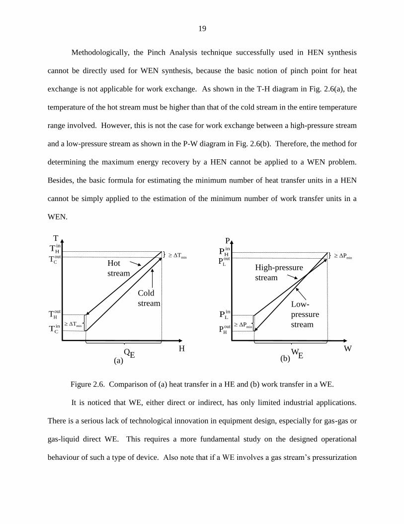
Methodologically, the Pinch Analysis technique successfully used in HEN synthesis
cannot be directly used for WEN synthesis, because the basic notion of pinch point for heat
exchange is not applicable for work exchange. As shown in the T-H diagram in Fig. 2.6(a), the
temperature of the hot stream must be higher than that of the cold stream in the entire temperature
range involved. However, this is not the case for work exchange between a high-pressure stream
and a low-pressure stream as shown in the P-W diagram in Fig. 2.6(b). Therefore, the method for
determining the maximum energy recovery by a HEN cannot be applied to a WEN problem.
Besides, the basic formula for estimating the minimum number of heat transfer units in a HEN
cannot be simply applied to the estimation of the minimum number of work transfer units in a
WEN.
Figure 2.6. Comparison of (a) heat transfer in a HE and (b) work transfer in a WE.
It is noticed that WE, either direct or indirect, has only limited industrial applications.
There is a serious lack of technological innovation in equipment design, especially for gas-gas or
gas-liquid direct WE. This requires a more fundamental study on the designed operational
behaviour of such a type of device. Also note that if a WE involves a gas stream’s pressurization
T
H
Hot
stream
Cold
stream
in
HTout
CT
in
CT
out
HT
minTΔ
minTΔ
QE
P
W
High-pressure
stream
Low-
pressure
stream
in
HPout
LP
in
LP
out
HP
minPΔ
WE(a) (b)
minPΔ

20
or depressurization, the stream temperature can be changed considerably in operation. Therefore,
such a WEN should be designed with heat integration technology incorporated; thereby leading to
a hybrid exchange network.
WEN synthesis problems could be mathematically formulated and solved by MINLP
techniques. Other types of synthesis methods could be also attractive, especially if a WEN design
problem involves not too many high/low pressure streams, which is common. In such a case,
heuristic based methods may demonstrate advantages, as a derived solution structure becomes
explainable, which allows engineers to address some practical design issues that could be difficult
to formulate mathematically. Note that since heat-incorporated WEN system is structurally highly
interacted, its operation could be sophisticated in terms of system dynamics, control, and process
safety.
The essential purpose of WEN synthesis is to improve process sustainability. This is the
reason in addition to energy; economic conservation plays a key role in development of any new
technology. However, cost estimation of the direct work exchangers has not been studied for
different capacities and sizes similar to other unit operations such as compressors and heat
exchangers. The limited application of these devices in desalination processes could be defined
as the main reason. A pilot study of flow work exchangers for desalination processes by Cheng
and Fan (1968) is the only available source which discussed the cost of the unit for a specific
capacity. Thus, to investigate the economic feasibility of using direct work exchangers in chemical
processes, the development of a unique formula for cost estimation of the unit would be of great
importance.
Among different types of WEs, the Dual Work Exchange Energy Recovery Device
(DWEER) has been widely used for seawater reverse osmosis (RO) desalination, which is one of

21
the most efficient energy recovery systems developed to date (by Flowserve Corporation). This
type of device (dealing with liquid streams) has been reported to have low mixing and leakage
losses, low maintenance cost, and self-adjustment capability to different flow rates and pressures.
Despite that, WEs dealing with gas phase streams will demonstrate different operational
characteristics. Note that operational safety related to leakage and mixing losses should be
considered, especially when processing gas streams.
Another important concern is the operational performance of WEs, as the units may have
a longer cycle time, depending on the operational mode, in comparison to compressors and
expanders. Therefore, WEN dynamic control could be a challenge, as an effective operational
coordination strategy is needed for operating different types of units working in continuous or
batch-like operational modes. This requires a more comprehensive study on system control design.

22
CHAPTER 3 PREDICTION OF MAXIMUM RECOVERABLE MECHANICAL
ENERGY VIA WORK INTEGRATION: A THERMODYNAMIC MODELING AND
ANALYSIS APPROACH
The known studies have clearly shown that WEN, either using direct or indirect work
exchangers, is a new type of process network system for recovering mechanical energy that is
consumed or provided by compressors, pumps, turbines, and other types of pressure vessels.
However, there is still no known method that can be used to predict the maximum amount of
mechanical energy recoverable by work exchangers prior to process synthesis. As the pinch
concept is not valid in work exchange analysis, the traditional pinch analysis method is in general
not applicable for WEN synthesis. Thus, a new type of synthesis methodology should be
developed. As the first step, prediction of maximum recoverable mechanical energy prior to
network synthesis should be of great significance, as this could help determine if a WEN is
economically attractive for energy recovery, and if so, the predicted energy recovery can be set as
a target to achieve in the process synthesis phase.
In this chapter, we focus on introducing a mathematical modeling and analysis method
which aims at predicting the maximum amount of mechanical energy that can be feasibly
recovered using work exchangers. The modeling and analysis method can be applied to the design
of a work exchange system operated under isothermal or adiabatic conditions. To illustrate
methodological efficacy, two case study problems selected from the literature are investigated and
the results are compared with those by other methods.
3.1 Mathematical Framework for Energy Recovery Targeting
A WEN synthesis problem can be stated as follows. Given a set of high-pressure streams
(i
H , i = 1, 2, ···, HN ) and a set of low-pressure streams (j
L , j = 1, 2, ···, L
N ), their supply and
target pressures (i.e., s
H iP ,
t
H iP ,
s
L jP , and
t
L jP ), volumetric flowrates (i.e.,
iHV and jLV ), and the

23
minimum acceptable pressure difference between any pair of high-pressure and low-pressure
streams (i.e., minΔP ), synthesize a WEN that can recover the maximum amount of mechanical
energy at the lowest cost.
To set an energy target for this type of synthesis problem, we introduce a thermodynamic
modeling and analysis method that can be used to determine precisely the maximum amount of
mechanical energy recoverable by a WEN prior to flowsheet development. The modeling involves
an introduction of a number of matrices and vectors, which is followed by a model-based
computational procedure.
Identification of pressure intervals of low-pressure streams for pressurization by
high-pressure streams. This task can be accomplished in two steps.
Step 1. Construct matrix Γ . For each low-pressure stream Lj (j = 1, 2, ···, NL), it is
required to identify the largest pressure interval, within which Lj can receive mechanical energy
thermodynamically feasibly from each high-pressure stream Hi (i = 1, 2, ···, NH). Thus, we
introduce matrix Γ to accommodate all NH×NL intervals in the following structure:
LNHNHNHN
LN
LN
L,HL,HL,H
L,HL,HL,H
L,HL,HL,H
21
22212
12111
Γ , (3.1)
where
b
L,Ha
L,HL,Hjijiji
, , (3.2)

24
where ji
L,H is the identified pressure interval between streams Hi and Lj;
aL,H
ji
is the lower-
bound pressure; b
L,Hji
is the upper-bound pressure. Figure 3.1 shows a flowchart that can be
used to generate each pressure interval in the matrix, where the necessary condition for work
transfer between a pair of H and L streams shown in Eq. 2.5 is implemented.
Step 2. Construct matrix P . Note that within any specific pressure interval of a low-
pressure stream, it can accept energy from only one high-pressure stream. However, in matrix Γ ,
some identified interval(s) of an L stream may be associated with more than one H stream. If this
occurs, then the overlapped pressure range between the identified interval(s) should be specified;
only one such an interval can be kept, and the others should be excluded. Therefore, we introduce
another matrix named P (NH×NL), which should be derived through manipulating element values
in matrix Γ .
LNHNHNHN
LN
LN
L,HL,HL,H
L,HL,HL,H
L,HL,HL,H
PPP
PPP
PPP
21
22212
12111
P , (3.3)
where
b
LH
a
LHLH jijijiPPP ,,, , . (3.4)

25
Figure 3.1. Flowchart for derivation of matrix Γ .
i = 1, j = 1
PH < PL + ∆Pmin
Y
PL < PH - ∆Pmin < PL
N
j = NLj = j+1
i = NHi = i+1
Y
N
N
Y
N
N
Y
Y
Output matrix Γ
Input H and L stream data
i
s
j
t
?
j
s
i
sj
t
N
Y
= PH - ∆Pmini
s= 0 = PL j
t
= 0 = PL j
s
PL < PH + ∆Pmin < PLjs
i
tj
t
PL < PH + ∆Pminj
s
i
t
= PH + ∆Pmini
t
?
?
?
?
?
Lo
wer
-bound det
erm
inat
ion
( )
Upper
-bound det
erm
inat
ion
( )
α
L,Η jιΓ
α
L,Η jιΓ
α
L,Η jιΓ
b
L,Η jιΓ
b
L,Η jιΓ b
L,Η jιΓ
b
L ,Η
jι
Γα
L ,Η
jι
Γ
Construct Γ

26
The element, ji
L,HP can be determined in two sub-steps. The first sub-step is to calculate
lL,H
ji
P using the following formula:
otherwise
if
;R
VV;
P
jlijijiji
liiji
ji
L,HL,HL,HL,H
HHL,H
lL,H
(3.5)
where l is an index whose value should satisfy two conditions: (1) 0 but 1 l NlH
, and (2)
.NliH
0 Note that the long bar above the intersection of ji
L,H and
jlijiL,HL,H
R
in
the above equation is an operation of complement in set theory.
The second sub-step of the evaluation is to determine ji
L,HP , which is the intersection of
all identified s'Pl
L,Hji
, i.e.,
l
L,HL,Hjiji
PP . (3.6)
Note that jliji L,HL,HR in Eq. 3.5 is the overlapped pressure range between the
thji L,H interval and the th jli L,H interval in the j-th column of matrix Γ ; it can be
determined through performing the following operation:
b
L,H
b
L,H
a
L,H
a
L,HL,HL,H jlijijlijijliji,R
ΓΓΓΓ . (3.7)
Evaluation of mechanical energy transfer from high-pressure streams to low-
pressure streams. Using the pressure interval information in matrix P , we can calculate the

27
mechanical energy that can be transferred from each individual high-pressure stream to each
individual low-pressure stream. Matrix
W (H
N ×L
N ) is thus introduced to collect all energy
transfer data in a structured way, i.e.,
LNHNHNHN
LN
LN
L,HL,HL,H
L,HL,HL,H
L,HL,HL,H
WWW
WWW
WWW
21
22212
12111
W (3.8)
where
,
,
,
1
,
β
,
ρ; Isothermal condition
ρ1 ; Isentro
1
j j i j
j
i jL j
L
L
j j i j
H L ji j
i jL j
b
L L H Ls
L a
H Lw
k
b kL L H LsL
L a
L H Lw
V PzRT ln
M P
V PkW zRT
k M P
1
,
,
pic condition (adiabatic)
ρ1 ; Polytropic condition (adiabatic)
1
L
L
j j i j
j
i jL j
m
b mL L H LsL
L a
L H Lw
V PmzRT
m M P
(3.9)
Note that in the isentropic and polytropic conditions, the outlet temperature of a low-pressure
stream changes after each compression step. Hence, in calculation of ,WjL,iH
the inlet
temperature of low-pressure stream, ,T sL
i should be multiplied by
1
,
L
L
i j
j
k
a kH L
s
L
P
P
or
1
,
L
L
i j
j
m
a mH L
s
L
P
P
for
the isentropic or polytropic condition, respectively, in order to eliminate calculation error.
In matrix
W , the sum of the element values in any row (e.g., the i-th row) is the total
amount of mechanical energy from the corresponding high-pressure stream (i.e., i
H ) to all L
N

28
low-pressure streams (i.e.,
L
jL,iH
N
j
W
1
). This amount of energy required for pressurizing all the
low-pressure streams can be greater than, equal to, or less than the total amount of energy that the
high-pressure stream (i
H in this case) can transfer. Understanding the value difference is
important as this could affect design decision during flowsheet development. Here, a vector named
W ( 1
HN ) is defined to include this type of value information for each high-pressure stream.
HN
W
W
W
2
1
W , (3.10)
where
L
jL,iHii
N
jH
WWW
1
. (3.11)
According to Eqs. (T2.1-1), (T2.1-3), and (T2.1-5) in Table 2.1, the value of i
HW can be estimated
as follows:
1
; Isothermal condition
ρ1 ; Isentropic condition (adiabati
1
i i i
i
iHi
H
H
i i i
i i
iHi
s
H H H
H t
Hw
k
s kH H HtH
H H t
H Hw
V ρ PzRT ln
M P
V PkW zRT
k M P
1
c)
ρ1 ; Polytropic condition (adiabatic)
1
H
H
i i i
i
iHi
m
s mH H HtH
H t
H Hw
V PmzRT
m M P
(3.12)

29
Note that in the isentropic and polytropic conditions, the outlet temperature of high-
pressure stream, tH
i
T , will change after each stage of expansion, which can be evaluated as
follows:
1
1
; Isentropic condition (adiabatic)
; Polytropic condition (adiabatic)
H
H
i
i
i
i
H
H
i
i
i
k
t kHs
H s
H
t
H
m
t mHs
H s
H
PT
P
T
PT
P
. (3.13)
Determination of the minimum amount of external energy requirement. The element
values in vector
W can be positive, zero, and negative. The sum of all positive values in vector
W (i.e., 0
i
W
) is the total amount of mechanical energy of H
N high-pressure streams that
cannot be used for pressurizing feasibly low-pressure streams. This amount of energy should be
removed by expanders. We use variable UE
W to quantify this total external power for expanders,
i.e.,
H
i
n
i
UE
WW
1
, (3.14)
where i
W
included in the above equation must be of a positive value, and H
n is the total number
of the elements with a positive value each in vector
W .
On the other hand, if the i-th element in
W has a negative value, this means the energy
transferred from high-pressure stream i
H to L
N low-pressure streams is insufficient. The sum of
all the negative values in the vector
W is part, but not all, of the total demand of the external

30
compression power needed for pressurizing the low-pressure streams. This amount can be
evaluated by variable UC
W1
that is defined below:
H
i
n
i
U
C WW1
γ1, (3.15)
where i
W
included in the above equation must be of a negative value, and H
n is the total number
of elements having a negative value each in vector
W .
Note that matrix P contains the pressure intervals of low-pressure streams for feasibly
receiving mechanical energy from high-pressure streams. In general, there must be other pressure
intervals of low-pressure streams, within which no energy can be received from any high-pressure
stream, based on the necessary condition for feasible work exchange shown in Eq. 2.5. Thus, in
order to meet the pressurization requirement for those intervals, additional external compression
power will be needed. Variable UC
W2
is designated for this purpose; it can be calculated as follows:
tot
LHtotL
UC
WWW
2
, (5.16)
where totL
W is the total demand of all L
N low-pressure streams for pressurization, which can be
calculated as:
L
j
N
jL
totL
WW
1
, (3.17)
and totLH
W
is the total amount of energy that can be obtained by all low-pressure streams from all
high-pressure streams, which can be calculated as follows:
H L
j,i
N
i
N
j
totLH
WW
1 1
. (3.18)

31
Therefore, the total amount of external compression energy needed by pressuring the low-
pressure streams is:
U
C
U
C
U
C WWW21
. (3.19)
Estimation of the maximum amount of recoverable mechanical energy. The maximum
amount of mechanical energy that can be feasibly recovered from high-pressure streams is the
difference between the amount of mechanical energy to be removed from the high-pressure
streams and the minimum amount of external expansion utilities. Here we introduce variable
,W totR
which can be expressed as follows:
UE
totH
totR
WWW , (3.20)
where totH
W is the total amount of energy of all H
N high-pressure streams for depressurization,
which can be calculated as:
H
i
N
i
H
tot
H WW1
. (3.21)
On the other hand, this amount can be also expressed by evaluating the difference between
the total amount of mechanical energy needed by all low-pressure steams and the minimum
amount of external compression power evaluated in Eq. 3.19, i.e.,
U
C
tot
L
tot
R WWW . (3.22)
Calculation procedure. The models and evaluation methods described above can be
organized as a procedure, which is shown in Fig. 3.2. The procedure is general for a WEN
synthesis problem of any size. It can be readily coded as a computational program using Excel or
so (Appendix B). Note that in above formulations, construction of matrices Γ and P requires

32
more calculation steps. This will be illustrated in Case 1 in the following section. Calculation of
the remaining matrices and vectors using Eqs. 3.8 to 3.22 are straightforward.
3.2 Case Studies
Two case study problems selected from the open literature are investigated in this section,
in order to demonstrate the significance and efficacy of the introduced methodology. As stated,
the methodology is used to determine the maximum amount of mechanical energy
thermodynamically feasibly recoverable by a WEN prior to synthesis.
3.2.1 Case 1- Prediction of the Maximum Recoverable Mechanical Energy of a System
Operated under Isothermal Conditions
This design problem studied by Liu et al. (2014) involves three high-pressure streams and
two low-pressure streams. The process stream data is listed in Table 3.1.

33
Figure 3.2. Flowchart for evaluation of maximum recoverable mechanical energy.
Construct matrix
[Eqs. (3.1)-(3.2)]Γ
Construct matrix
[Eqs. (3.3)-(3.7)]P
Construct matrix
[Eqs. (3.8)-(3.9)]
Classify energy types
using [Eqs. (3.10)-(3.13)] γW
UE
W
Calculate [Eq. (3.15)]
Calculate [Eq. (3.14)]
U
CW1
Calculate
[Eqs. (3.16)-(3.18)]
Calculate
[Eq. (3.20) or (3.22)]
U
CW
tot
RW
W
U
CW2
Output calculated energy recovery results
Input system design data
Calculate [Eq. (3.19)]

34
The minimum acceptable pressure difference between any pair of high-pressure and low-
pressure streams (i.e., ∆Pmin) is 70 kPa. It is assumed that each stream is an ideal gas, and the work
transfer units are operated under isothermal condition. It is also assumed that the process
operational efficiency is 100%.
Table 3.1. Process stream data for Case 1
Stream
No.
Supply pressure
(Ps, kPa)
Target pressure
(Pt, kPa)
Volumetric flowrate
(V, Nm3/s)
Inlet temperature
(Ts, K)
H1 2,000 150 1.23 525
H2 780 180 0.57 480
H3 780 220 0.85 420
L1 200 700 1.85 330
L2 200 1,600 0.83 360
Γ is a 23 matrix as follows:
2313
2212
2111
,LH,LH
,LH,LH
,LH,LH
ΓΓ
ΓΓ
ΓΓ
Γ . (3.23)
Among the six elements in the matrix, we show the calculation of only three elements,
11 L,HΓ , 13 L,HΓ , and 22 L,HΓ , as the derivation of these element values can demonstrate different
ways of calculation shown in the flowchart of Fig. 3.1.
a) Evaluation of .Γ11 L,H This requires calculation of the lower- and upper-bound values
of the interval.
a-1) Calculation ofa
L,H 11Γ . Since
1
s
LP (200 kPa) is less than the sum of 1
t
HP (150 kPa) and
∆Pmin (70 kPa), which is further less than 1
t
LP (700 kPa), we have:
kPa 22070150Δ min111 PPΓ t
H
a
L,H . (3.24)

35
a-2) Calculation of b
L,H 11Γ . Note that
1
s
HP (2,000 kPa) is greater than the sum of 1
t
LP (700
kPa) and ∆Pmin (70 kPa). Thus,
1 1 1
b t
H ,L LΓ P 700 kPa . (3.25)
Therefore,
007 22011
,Γ,LH . (3.26)
b) Evaluation of .Γ1L,H3 This also requires calculation of the lower- and upper-bound
values of the interval.
b-1) Calculation ofa
L,H 1Γ
3. As
1
s
LP (200 kPa) is less than the sum of 3
t
HP (220 kPa) and
∆Pmin (70 kPa), which is further less than 1
t
LP (700 kPa), we have:
kPa. 29070220Δ min313 PPΓ t
H
a
L,H (3.27)
b-2) Calculation of b
L,H 1Γ
3. Note that
3
s
HP (780 kPa) is greater than the sum of 1
t
LP (700
kPa) and ∆Pmin (70 kPa). Thus,
kPa 70013
t
L
b
L,H jPΓ . (3.28)
Thus,
007 29013
,Γ L,H . (3.29)
c) Evaluation of .Γ L,H 22 Again, the lower- and upper-bound values of the interval should
be separately calculated.
c-1) Calculation ofa
L,HΓ 22. Since
s
LP2 (200 kPa) is less than the sum of
t
HP2(180 kPa) and
∆Pmin (70 kPa), which is further less than t
LP2 (1,600 kPa), we have:

36
2 2 2, minΔ 180 70 250 kPaa t
H L HΓ P P . (3.30)
c-2) Calculation of b
L,HΓ 22. Note that
s
HP2 (780 kPa) is less than the sum of
t
LP2 (1,600 kPa)
and ∆Pmin (70 kPa). Moreover, s
LP2 (200 kPa) is less than the difference between
s
HP2 (780 kPa) and
∆Pmin (70 kPa) and further less than t
LP2 (1,600 kPa). This gives rise to the following:
2 2 2
b s
H ,L H minΓ P Δ 780 70 710 kPaP . (3.31)
Thus,
107 250 ,Γ22 L,H . (3.32)
d) Construction of a complete matrix Γ . By referring to the calculation examples above,
three other elements in matrix Γ can be readily derived. The following matrix shows a complete
element calculation result:
220,700 220,1,600
250,700 250,710
290,700 290,710
Γ . (3.33)
Matrix P has the same dimension as matrix Γ , i.e.,
2313
2212
2111
,LH,LH
,LH,LH
,LH,LH
PP
PP
PP
P . (3.34)
In the following derivation, we show how to calculate two elements, 11,LHP and 12,LHP .
Calculation of other four elements can be performed in the same way.
a) Calculation of 11
L,HP . This interval is derived from interval
11L,H
Γ . According to
Eq. 3.5, the value of index l should be determined first; it must satisfy two conditions: (1)

37
0 but 1 l Nl H , and (2) ,0H
Nli where 3H
N . Based on the first condition, l can
be 2, 1, -1, or -2. However, based on the second condition, i should be 1 (referred to 1
H ). Thus,
l’s value of -1 or -2 is not valid. Therefore, we just need to evaluate 1
11 L,HP and .P L,H
2
11 In this
case, 1
HV (1.23 Nm3/s) is greater than
2H
V (0.57 Nm3/s). Thus, we have:
700 220,1111 L,H
1
L,H ΓP . (3.35)
Since 1HV (1.23 Nm3/s) is greater than
3HV (0.85 Nm3/s). Thus, we also have:
700 220,2
1111 L,HL,H ΓP . (3.36)
Therefore, using Eq. 3.6 gives:
700220 ,P ,PP2
L,H
1
L,HL,H 111111 (3.37)
b) Calculation of 12 L,HP . This interval is derived from 12 ,LHΓ . The values of index l should
be decided, based on two conditions: (1) 0 but 1 l Nl H , and (2) .Nli H0 Again,
based on the first condition, l can be 2, 1, -1 or -2. However, based on the second condition, i = 2
(referred to 2
H ), l’s value can be only -1 or 1. Therefore, we just need to evaluate 1
L,H 12P
and
1
L,H 12P . Note that since
2H
V (0.57 Nm3/s) is less than 1
HV (1.23 Nm3/s), the following calculation
is performed based on Eq. 3.5:
007 250700700220250
,,
ΓΓ,ΓΓ R bL,H
bL,H
aL,H
aL,HL,HL,H
111211121112
(3.38)
Then,

38
.,,,,
,,,,,P1
L,H12
00 700250700250
700250700250 700250700250700250
(3.39)
Since 2
HV (0.57 Nm3/s) is less than
3HV (0.85 Nm3/s), the following calculation should be
performed based on Eq. 3.5:
.,,
ΓΓ,ΓΓ R bL,H
bL,H
aL,H
aL,HL,HL,H
112112112
007 290700700290250
333
(3.40)
Then,
.,,,,
,,,,,P12
L,H
902 250 700290700250
700290700250 7002907002507002501
. (3.41)
Therefore,
0 0,P,PP1
L,H
1
L,HL,H 121212
. (3.42)
c) Construction of a complete matrix P . Using the same approach, we can calculate the
values of four other elements in matrix P . All these values are assembled as follows:
0000
0000
1600220700220
,,
,,
,,
P . (3.43)
Using Eqs. 3.8 and 3.9, we can obtain matrix
W (3×2) as follows:
00
00
9221912262
β
..
W . (3.44)

39
As shown, the mechanical energy of stream H1 will be transferred to streams 1
L and 2
L , but
streams 2
H and 3
H will not transfer any. Note that for the high-pressure streams, the amounts of
mechanical energy available can be calculated using Eq. 3.12 as: 486201
.WH
kW,
821482
.WH
kW, and 611673
.WH
kW. With this information, we are able to derive the values
of vector γW , using Eqs. 3.10 and 3.11, i.e.,
61167
82148
43138
3
2
1
.
.
.
W
W
W
γ
W . (3.45)
In the above vector, 1
W (138.43 kW) is the remaining amount of energy of stream 1
H after
transferring 262.12 kW to stream 1
L and 219.92 kW to stream 2
L . The sum of the three element
values in vector
W is the total amount of mechanical energy of the three high-pressure streams
that cannot be used to pressurize any low-pressure stream. Thus, we can calculate the amount of
external expansion energy provided by the system using Eq. 3.14, which gives:
W 138.43 148.82 167.61 454.86 kWU
E . (3.46)
Using Eqs. 3.15 to 3.19, we can obtain the following:
0UC
1
W , (3.50)
and
2
514.19 482.04 32.15 kWU
CW . (3.51)
Therefore, the minimum amount of external compression energy needed for the system is:
1 2
32.15 kWU U U
C C CW W W . (3.52)

40
Now we can calculate the maximum amount of mechanical energy that can be recovered
by a WEN using Eqs. 3.20 and 3.21, i.e.,
(620.48 148.82 167.61) 454.86 482.05 kWtot tot U
R H EW W W . (3.53)
The same result can be obtained using Eq. 3.22, i.e.,
(283.71 230.49) 32.15 482.05 kWtot tot U
R L CW W W . (3.54)
Table 3.2 summarizes the benefit of mechanical energy recovery using a WEN. It is shown
that a WEN can recover 93.75% of the energy for stream compression, and 51.45% of the energy
for stream expansion.
Table 3.2. Energy recovery analysis for Case 1
External
utility type
External energy requirement (kW) Energy recovery
by WEN (%) Without WEN Using WEN
Compression 514.19 32.15 93.75
Expansion 936.91 454.86 51.45
As a separate effort from this work, we have successfully synthesized a WEN for this
design problem using a methodology that we developed, which is shown in Fig. 3.3(a). Since
network synthesis is beyond the scope of this chapter, derivation of a process flowsheet is not
discussed here. In the derived network, the maximum mechanical energy recovery predicted by
the introduced methodology (482.05 kW) is indeed achieved. The network contains two work
exchangers, two compressors, and three expanders. As a comparison, the solution derived by Liu
et al. (2014) is plotted in Fig. 3.3(b). In their solution, four work exchangers are used to recover
a total of 367.56 kW of mechanical energy, which is 23.75% less than the maximum recoverable
mechanical energy that was predicted. In addition, the number of compressors and expanders used
in their solution is larger than that in our solution. The comparison of energy recovery and process
unit requirement is summarized in Table 3.3.

41
Table 3.3. Performance comparison of WENs by different methods for Case 1
Solution
Energy recovery efficiency (%) Number of
work
exchangers
Number of utility units
Compression Expansion Compressor Expander
Fig. 3.3(a), by
this work 51.45 93.75 2 2 3
Fig. 3.3(b), by
Liu et al. (2014) 39.23 71.48 4 3 5
3.2.2 Case 2 – Prediction of the Maximum Recoverable Mechanical Energy of a System
Operated under Adiabatic Conditions
Razib et al. (2012) studied an interesting WEN design problem, where single-shaft-turbine-
compressor (SSTC) units, instead of (direct) work exchangers introduced in this work, were used
for mechanical energy recovery. In their work, a superstructure for WEN configuration was
proposed and a mixed-integer nonlinear programming (MINLP) model was described for
identifying an optimal solution in terms of minimum total annualized cost. Their design problem
is selected for our case study, aiming at identifying the maximum amount of recoverable
mechanical energy. Table 3.4 lists the data of the synthesis problem. The minimum acceptable
pressure difference between any pair of high-pressure and low-pressure streams (i.e., ∆Pmin) is 70
kPa. It is assumed that each stream is an ideal gas, and the work transfer units are operated under
adiabatic conditions. It is also assumed that the process operational efficiency is 100%.

42
Figure 3.3. Work exchange networks designed by different methods for Case 1: (a) the solution
by the proposed model-based method to achieve the maximum energy recovery, and (b) the
solution derived by Liu et al. (2014).
[2000]
[780] [180]
[150]
[700]
[1600]
[200]
[200]
(219.92)
[220][780]
[220]
[220]
(262.12)
(167.61)
(148.82)
(10.56)
(21.58)
(138.43)
1H
2H
3H
1L
2L
W1
W1
W2
W2
E1
E2
E3
C1
C2
[2000]
[780] [180]
[150]
[700]
[1600]
[200]
[200]
(70.15)
[220][780]
[290]
[290]
(97.73)(21.53)
(148.82)
(41.21)
(84.19)
(155.53)
1H
2H
3H
1L
2L
W1
W1
W4
W4
E1
E4
C3
C2
E2
(75)
E3
W3
W3
C1
W2
W2
[850] [700]
[760] [220]
(69.06)
(91.8)
(130.62)
(98.55)
E5
Legend Work exchanger
Expander
[ ] : Pressure (kPa)
( ) : Work load (kW)
W
C Compressor E
(a)
(b)

43
Table 3.4. Process stream data for Case 2
Stream
No.
Supply
pressure
(Ps, kPa)
Target
pressure
(Pt, kPa)
Flowrate
(kg/s)
Source
temperature
(Ts, K)
Target
temperature
(Tt, K)
Heat
capacity
(CP, kJ/kg.k)
H1 850 100 3 600 430 1.432
H2 960 160 5 580 300 0.982
H3 800 300 2 960 300 1.046
L1 100 510 3 300 700 1.432
L2 100 850 3 300 600 1.432
Following the procedure in Figs. 3.1 and 3.2, we can derive the element values of matrices
Γ and P that are listed below.
170, 510 170, 780
230, 510 230, 850
370, 510 370, 730
Γ , (3.55)
and
0 00 0
850 230510 230
230 170230 170
,,
,,
,,
P . (3.56)
As shown, the element values in the last row of matrix P are all zero. This means that
high-pressure stream 3
H will not transfer energy to any low-pressure stream.
Following the same procedure, we can derive matrix
W , which contains the information
about the mechanical energy transferrable between any pair of high-pressure stream and low-
pressure stream. This matrix is derived as:
00
22448122803
9023126237
.,.
..
W (3.57)

44
The mechanical energy that should be removed from each high-pressure stream can be
evaluated using Eqs. 3.12 and 3.13: 5004411
.,WH
kW, 8030812
.,WH
kW, and 804173
.WH
kW. Having these data, together with the data in matrix
W , we can derive vector γW using Eqs.
3.10 and 3.11 as follows:
80417
64942
33575
3
2
1
.
.
.
W
W
W
γ
W . (3.58)
Different from Case 1, this vector contains one negative number. This means stream 2
H
does not have enough energy to be transferred to streams 1L and 2L . This amount (942.64 kW)
can be only obtained from an external compression power source (see Eq. 3.15), i.e.,
942.64 kW1
U
CW . (3.59)
This is, however, not the total demand of external compression power. This other portion
is ,2
UC
W which can be calculated using Eqs. 3.16-3.18 as follows:
23,406.10 237.26 231.90 803.22 1,488.22
685.49 kW.
U tot tot
C L H LW W W
(3.60)
Therefore,
1,628.13 kW1 2
U U U
C C CW W W . (3.61)
As to the minimum requirement of the external expansion power, it can be readily obtained
using Eq. 3.14; the result is:
1 3γ γW W W 575.33 417.80 993.13 kWU
E . (3.62)

45
Based on the results obtained above, we can calculate the maximum amount of recoverable
mechanical energy using either Eq. 3.20 or 3.22, i.e.,
1,044.50 1,308.80 417.80 993.13 1,777.97 kWtot tot U
R H EW W W , (3.63)
or
1,386.60 2,019.50 1,628.13 1,777.97 kWtot tot U
R L CW W W . (3.64)
As shown in Table 3.5, the total amount of work exchanged is 1,777.97 kW, accounting
for 52.20% of the total energy demanded by the two low-pressure streams, and 64.16% of that
provided by all high-pressure streams. This is a very significant contribution to energy reccovery.
Table 3.5. Energy recovery analysis for Case 2
External
utility type
External energy requirement (kW) Energy recovery
by WEN (%) Without WEN Using WEN
Compression 3,406.10 1,628.13 52.20
Expansion 2,771.10 993.13 64.16
To demonstrate the achievability of the predicted maximum energy recovery in design, we
have synthesized a WEN, which is plotted in Fig. 3.4(a). Since network synthesis is beyond the
scope of this chapter, we do not describe the synthesis methodology here. As shown in Fig. 3.4(a),
the energy target of recovering 1,777.97 kW is achieved using four work exchangers. This network
also contains three compressors and two expanders. Note that since the
pressurization/depressurization operation occurs under adiabatic conditions, the temperatures of
the process streams leaving work exchangers, compressors, and expanders will change. Therefore,
there is a need to consider recovery of thermal energy through integrating a heat exchanger
network (HEN). In Fig. 3.4(a), three hot streams (marked as HS1 – HS3) and two cold streams
(marked as CS1 and CS2) are identified, which define a HEN design problem. A synthesized HEN

46
is shown in Fig. 3.4(b). This network can recover 36.7% of thermal energy from hot streams
(645.95 kW out of 1,759.1 kW).
In Razib et al. (2012), a WEN is proposed using single-shaft-turbine-compressor (SSTC)
units, which is different from the work exchanger introduced in this work. Since their synthesis
target was to minimize the total annualized cost, a trade-off between the capital cost and operating
cost was made. Therefore, a complete comparison between our solution and their solution is not
approriate. However, a partial comparison is possible, which is summarized in Table 3.6. As
shown, our solution can recover more mechanical energy. Besides, our solution compares well
with their solution, in terms of the number of work transfer units (direct work exchangers in our
solution versus SSTCs in their work, compressors and expanders) as well as the number of heaters
and coolers.
Table 3.6. Performance comparison of WENs by different methods for Case 2
Type of device
used in WEN
Mech.
energy
recovered
(kW)
High-
pressure
recovery
(%)
Low-
pressure
recovery
(%)
No. of
exchan-
ger
units
No. of
heaters
and
coolers
No. of
external
compre-
ssors
No. of
external
turbines
Direct work
exchanger 1,778 64.16 52.20 4 5 3 2
SSTC, in
Razib et al.
(2012)
1,573 56.77 46.19 7 11 2 3

47
Figure 3.4. Flowsheet of heat-integrated work exchange network for Case 2: (a) work exchanger
network, and (b) heat exchanger network.
[850]
[960][160]
[100]
[510]
[850]
[100]
[100]
(803.22)
[300][800]
[170]
[170]
(237.26)
(417.8)
(942.64) (339.37)
(346.12)
(575.33)
1H
2H
3H
1L
2L
W4
W4
W3
W3
E2
C1
E1
C2
C3
{600}
{580}
{960}
{700}
{600}
{430}
{300}
{300}
{300}
{300}
W1
W2
W2
W1
{357}
{313}
{760}
{380}
{770} {379}
[370]
{551}
{623}
(505.58) (231.90)
[230]
{436}
[230]
{433}
CS1
HS1
HS2
HS3
CS2
<314.17>
1HS
2HS
3HS
1CS
2CS
{313}
{760}
{770}
{430}
{700}
{300}
{300}
{600}
{357}
{623}
HE1
HE2
HE1
{610.10}
{692.74}
<331.78>
HE2
<398.41>
<648.74>
<66>
4.30
4.91
2.09
4.30
4.30
CL1
CL2
CL3
Legend
Work exchanger
Expander
[ ] Pressure (kPa)
Heat transfer unit(s)
to be placed
W C Compressor
E
{ } Temperature (K) ( ) Work load (kW)
HE CLHeat exchanger Cooler
MC (kW/K)P < > Heat load (kW)
(a)
(b)

48
3.3.3 Discussion
As stated, the case studies are presented to demonstrate that the maximum amount of
recoverable mechanical energy predicted by the introduced model-based methodology is
achievable during the process flowsheet development phase. It is shown that the WENs derived
in the case studies can recover more mechanical energy than those known designs in the open
literature. In addition, the work transfer units used in each derived network are fewer than those
in the known ones. Thus, energy target setting before WEN synthesis is highly desirable. The
introduced model-based energy prediction methodology should be a valuable tool for process
designers.
Although the derived WENs in the case studies are better solutions than known ones, the
solution optimality cannot be ensured here. There may be other configurations that can also
achieve the energy recovery goal at the lowest total annualized cost. Optimal process flowsheet
development requires a sophisticated synthesis methodology, which is beyond the scope of this
chapter.
3.4 Summary
Mechanical energy recovery is a very important issue in energy efficiency improvement in
the chemical process industry. However, this has drawn attention only in recent years. Apparently,
significant effort on methodological and applied research is needed. Since the operational mode
of the introduced (direct) work exchanger is very different from traditional heat transfer units,
Pinch Analysis, which is a mature methodology for heat exchanger network (HEN) synthesis, is
not directly applicable for work integration. Thus, a class of entirely new methodologies for work
exchanger network (WEN) synthesis is needed.

49
To facilitate WEN synthesis, we have introduced a thermodynamic modeling and analysis
methodology for predicting the recoverable mechanical energy prior to process flowsheet
development. The methodology is rigorous and general for a synthesis problem of any size, and
it can be used for work exchange operations under isothermal, isentropic, or polytropic conditions.
Case studies have shown that the energy targets are set precisely, and they are achievable in the
process flowsheet development stage. The comparison with the solutions in the open literature
has demonstrated the efficacy of the introduced methodology.
Note that when a WEN is operated under adiabatic conditions, process stream temperatures
through different work transfer units will be changed within the system. In such a case, heat
integration technology should be used to design a HEN in order to ensure the efficiency of thermal
energy recovery as well. Since energy efficiency is of utmost importance in the chemical process
industry, it is conceivable that significant progress on the research for simultaneous recovery of
mechanical and thermal energy will be made in the near future.

50
CHAPTER 4 SYNTHESIS OF COST EFFECTIVE HEAT INTEGRATED WORK
EXCHANGE NETWORK
A mathematical modeling and analysis method was introduced in Chapter 3 to predict the
maximum amount of mechanical energy that can be feasibly recovered using direct work
exchangers prior to WEN configuration development (Amini-Rankouhi and Huang, 2017). As the
next step towards completion of WEN synthesis, a comprehensive methodology is required. Also,
due to temperature and pressure correlation in gas phase streams, recovery of thermal energy
through heat integration will significantly impact the amount of energy recovery and total
annualized cost. In this chapter, we will introduce a thermodynamic model-based synthesis
approach to develop a heat-integrated work exchanger network (HIWEN), in which direct work
exchangers may work under different operating conditions. Case studies will demonstrate that the
resulting HIWENs can recover the maximum amount of mechanical and thermal energy at the
lowest cost.
4.1 Work Exchanger Network Synthesis Methodology
In the following, we will introduce a work exchanger network synthesis methodology
which will allow us to develop the flowsheet after the prediction stage. The flowsheet can be
combined with heat exchanger networks that are integrated before or after the WEN synthesis.
The location of HEN network is assigned based on the design with the lower operating cost. In
the end, the design can be modified using an adjustment instruction.
Flowsheet development procedure. For any specific case study with given information,
after determination of the maximum recoverable energy through the prediction methodology,
variables NH, NL and matrices P , HW , LW , βW , and γW will be used as inputs for the synthesis
stage. Figures 4.1 and 4.2 show the procedure in detail for final flowsheet development.

51
Placement of work exchangers using matrices WW and MP . As discussed in Chapter
3, Matrix βW represents the amount of mechanical energy that can be feasibly transferred from
each individual high-pressure stream to each individual low-pressure stream. However, the
amount of energy each high-pressure stream can provide could be higher or lower based on the
vector γW . Therefore, to generate WW which is the matrix of work exchanger workloads between
i-th high-pressure stream and j-th low-pressure stream, matrix βW and vector LW would be the
best options to find the most appropriate location for work exchangers. Any positive term from
vector γW shows that the i-th high-pressure stream can provide sufficient mechanical energy to
the low-pressure streams it is assigned to through the preparation of matrices P and βW . Based
on the flowchart shown in Fig. 4.1, while i
Wγ
has a positive value or its absolute value is less than
jL,iHWβ , a work exchanger should be placed with workload equal to
jL,iHWβ . While
i
Wγ
has a
negative value and its absolute value is higher than jL,iH
Wβ , a work exchanger should be placed
with workload equal to ijL,iH
WWγβ unless
jL,iHWβ is the largest number in the j-th column.
Therefore, we can introduce matrix WW to accommodate work exchangers with highest workloads
in the following structure:
LNL,HNHL,
HNHL,HNH
LNL,HL,HL,H
LNL,HL,HL,H
WWW
WWW
WWW
W
WWW
WWW
WWW
21
22212
12111
W , (4.1)

52
Generation of matrix MP . Each term in matrix MP defines the range of each low-
pressure stream which will receive energy from each high-pressure stream in the range of s
H
t
H iiP,P
. Therefore, after construction of matrix MP , for each term, one work exchanger will be placed
between s
H
t
H iiPP , and
H , L H , Li j i j
a b
M MP , P
with energy to be exchanged in amount of jL,iH
WW . Note
that based on this methodology, each high-pressure stream may transfer energy in the range of
s
H
t
H iiPP , to more than one low-pressure stream which means that there will be splitting in high-
pressure streams under this condition. Matrix MP which contains NH×NL intervals will be
structured as follows:
1 1 1 2 1
2 1 2 2 2
1 2
H ,L H ,L H ,LNL
H ,L H ,L H ,LNL
H ,L H ,L H ,LN N N NH H H L
M M M
M M M
M M M
P P P
P P P
P P P
MP , (4.2)
where
b
M
a
MMjL,iHjL,iHj,LiH
P,PP . (4.3)
To determine element j,LiH
MP , the upper-bound of the interval will be assumed equal to the
upper-bound of the interval ji ,LHP , and the lower-bound will be calculated based on the workload
of the assigned work exchanger. Then,
b
L,H
b
M jijL,iH
PP , (4.4)
and

53
1
1
exp ; Isothermal conditionρ
ρ
1
H , Li j
H , Li j
j j
j
L j
L
LL
H , Li jL
H , L H, Li j
L
Wb
M
L Ls
L
w
k
s kkLWka b
M M
sL L LL
L w
WP
VzRT
M
W PP P
k VzRT
k M
1
1
1
1
; Isentropic condition (adiabatic)
; Polytropic condition (adiabatic)
ρ
1
L
L
L
L
L
LL
H , Li jL
H, L
L
k
k
m
m
m
s mmLWmb
M
sL L LL
L w
W PP
m VzRT
m M
(4.5)
Note that for cases which a heat exchanger network will be located before the work
exchange network, the formulation shown in Eq. 4.5 will be slightly changed. The formulation
will be discussed later.
Placement of compressors using vectors 1CW and
2CW . Vector 1CW represents the
compressors that are required when the high-pressure streams are not able to provide enough
energy for each specific low-pressure stream even under thermodynamically feasibility conditions.
At this stage, one or more compressors with a total workload of j1CW will be placed in the j-th low-
pressure stream for the regions that still require pressurization. Thus, vector 1CW will be structured
as follows:

54
LN
C
C
C
W
W
W
1
21
11
1CW , (4.6)
where
H
jL,iHjL,iHj
N
iWC
WWW1
β1
. (4.7)
Each term in the j-th row of vector 2CW represents placement of one or two compressors
in the j-th low-pressure stream, which cannot receive energy from any high-pressure stream
because of thermodynamic feasibility conditions ( minΔin out
H LP P P and minΔin out
L HP P P ) which
was assigned from the initial step of prediction stage in the construction of matrices Γ and P .
Comparing the pressure interval of the j-th column in matrix P with the supply and target
pressures of the j-th low-pressure stream (i.e., t
L
s
L jjPP , ), the compressors can be placed in the
beginning/end of the j-th low-pressure stream with a total workload of 2
CWj
.
LN
C
C
C
W
W
W
2
22
12
2CW , (4.8)
where
H
jL,iHj
j
N
iLC
WWW1
β2
. (4.9)

55
Placement of expanders using vector EW . Any positive value in the vector γW
represents the amount of energy that the i-th high-pressure stream cannot provide to any low-
pressure stream and an external expander should be placed. Therefore, the vector EW will be
constructed based on the values from vector γW . Each non-zero value in vector EW defines
placement of one expander in the range of s
H
t
H iiPP , in the amount of
iEW in the i-th high-pressure
stream. For high-pressure streams which are also transferring energy to a low-pressure stream
through work exchange and still requires an expander, there will be stream splitting.
LN
E
E
E
W
W
W
2
1
EW , (4.10)
where
0 ;
0 0
γγ
γ
ii
i
i WW
W;W
E. (4.11)
The four final outputs of the flowcharts shown in Figs. 4.1 and 4.2 which are matrices and
vectors will provide the information for the placement of the unit operations such as work
exchangers, external compressors, and external expanders. However, for an energy efficient and
cost effective design, integration of heat into the work exchanger network design and also capital
and operating cost estimation should be analyzed.

56
Figure 4.1. Generation of WW and MP .
i = 1, j = 1
j = NLj = j+1
i = NHi = i+1
N
Y
N
N
Y
Input
?
N
?
?
?
Construct WW
iγ
W 0
ijL,iHWW
γβ Y
ji ,
Wβ= max{
ji ,
Wβ
| LNj ,,, 21 } ?
Y
jL,iHWWijL,iH
WWγβ =
jL,iHWWjL,iH
Wβ=
Y
HNLN P
HW LWβW γW
, , ,
,,,
N
A
Gen
erat
ion
of
WW
Countif ( ?=1
N
YLNj ,,, 21|
jL,iHWβ iγ
W )
j = NLj = j+1
i = NHi = i+1
?N
=
Y
i = 1, j = 1
?
Y
Construct
jjL,iH LW VW,f b
M
a
MjL,iΗjL,iΗ
PP
N
Gen
erat
ion o
f
MP
MP
b
L,Η jιP
b
MjL,ιΗ
P

57
Figure 4.2. Generation of 1C
W , 2C
W ,and EW .
4.2 Heat Integrated Work Exchange Network Design
Temperature change after each stage of pressurization and depressurization cannot be
neglected in real industrial cases. In the study by Deng et al. (2010), it was shown that applying
gas phase streams in work exchangers requires significant attention in comparison to liquid streams
j = NLj = j+1 ?
Construct 1CW
jC
1
W =
j = 1
jC
2
W =
N
Y
2CW,
A
Output , , ,
1C
W
2C
WWW
EW
Gen
erat
ion
of
W
,W
C1
C2
,MP
i = 1
i = NHi = i+1
Y
N?
?
iγ
W 0
iEW =
N
0iE
W =iγ
W
Construct EW
Y
Gen
erat
ion
of
WE
H
jL,iHj
N
iL
WW1
β
H
jL,iHjL,iH
N
iW
WW1
β

58
especially due to temperature dependence. This is the reason, in processes under the adiabatic
condition where the outlet temperature after each stage of pressurization or depressurization is not
the desired temperature and needs to be heated or cooled based on the streams specification, heat
integration should be taken into consideration in addition to work integration. With a derived
WEN flowsheet, the process streams with different temperature profiles will be identified, and a
corresponding thermal energy recovery system will be synthesized.
For design problems with one or more streams with given target temperature. When
dealing with streams in the gas phase, temperature plays a key role in the amount of energy that is
required for compression or provided through expansion. Depending on the design problem, a
target temperature may or may not be specified. For the cases where the outlet temperature of the
pressurization/depressurization stage is different from the target temperature, heating or cooling is
required. In such cases, the heat exchanger network (HEN) can be developed to recover thermal
energy to minimize the external heating and cooling utilities. To prevent complexity of the
solution development, HEN can be placed before or after the WEN. Figure 4.3 shows a flowchart
on how to develop HEN before/after WEN and decide the location based on the lowest operational
cost. In this stage, the prediction methodology presented in chapter 3 will be used to estimate the
amount of mechanical energy that will be recovered, and external compression and expansion
utilities. Thermal energy recovery and external heating and cooling will be estimated using the
temperature interval and cascade diagram of pinch analysis (Linnhoff and Flower, 1978). Note
that the shaft work formulation in the prediction methodology will differ based on the HEN
location.

59
Figure 4.3. Flowchart for HEN location decision making.
(a) When a heat exchanger network will be assumed before the work exchanger network,
the target temperature of high-pressure and low-pressure streams will be assumed constant and
inlet temperatures of the streams to the WEN system will be calculated based on the target
temperature provided by the problem design. As an example, iT shown in Fig. 4.4(a) can be
calculated as follows for each individual high-pressure and low-pressure stream under polytropic
(adiabatic frictional) conditions for ideal gas streams:
H
H
m
m
s
H
t
H
t
HH
i
P
P
TT
1
, (4.12)
and
Raw Design Data
Assume HEN before WEN
Use stream output temperature
to predict WEN energy
Assume HEN after WEN
Use stream input temperature
to predict WEN energy
Formulate an HEN problem Formulate an HEN problem
Estimate thermal energy for
HEN
Estimate total opt. cost based
on total utility consumption
Estimate thermal energy for
HEN
Estimate total opt. cost based
on total utility consumption
Compare two cases to find the
one which is cheaper
Announce the HEN location

60
L
L
m
m
s
L
t
L
t
LL
i
P
P
TT
1
. (4.13)
Therefore, for shaft work calculation used in the prediction and synthesis stages, target
temperatures given for each individual stream should be replaced by supply temperatures. In Table
4.1, changes that will be made in the formulation of the prediction and synthesis stages for
polytropic condition (frictional adiabatic) have been summarized.
Figure 4.4. (a) HEN located before WEN design, and (b) HEN located after WEN design.
After estimation of iT and calculating new UE
W , U
CW , and R
totW values for the WEN design
where the HEN is located before WEN, hot and cold streams will be derived and using pinch
analysis, the total amount of thermal energy that can be recovered in addition to total external hot
and cold utilities will be calculated. In the next stage, operating cost (OPEX ) using Eq. 4.14 will
be calculated.
HTLTL
jj
N
i
nCW
N
i
msteam
N
j
CCelec QCQCWWCOPEX111
21
(4.14)
where elecC is the cost of electricity ($/kWh), steamC is the cost of steam used as a heating utility
($/kWh), CWC is the cost of cooling water used as a cooling utility, mQ and nQ represent the heat
HEN
tPWEN
sPsT
tT
iTHEN WEN
sPsT
outT
tPtT
(a)
(b)

61
duty of the heating and cooling utilities, respectively. LTN is the total number of streams required
for heating and HTN is the total number of streams required for cooling.
(b) When a heat exchanger network will be assumed after the work exchanger network, the
supply temperature of high-pressure and low-pressure streams will be assumed constant and outlet
temperature of the streams leaving the WEN system will be calculated based on the supply
temperature provided by the problem design as shown in Fig 4.4(b). Each stream temperature that
will go through stages of pressurization or depressurization will increase or decrease, respectively.
Equations 4.15 and 4.16 show a calculation example under polytropic (adiabatic frictional)
conditions for ideal gas streams:
H
H
m
m
s
H
t
Hs
H
H
outP
PTT
1
, (4.15)
and
L
L
m
m
s
L
t
Ls
L
L
outP
PTT
1
. (4.16)
While the target temperature is specified for a case study, heating or cooling may be
required to reach the target temperature from H
outT and L
outT . Heat exchanger networks will be
integrated to recover the thermal energy of the heating and cooling utilities. The amount of
mechanical energy that can be recovered and external utilities ( UE
W ,U
CW , and R
totW ) will be
calculated using prediction methodology. Hot and cold streams will be derived to conduct the
pinch analysis and the operating cost will be calculated using Eq. 4.14.
Comparing the final operating cost from the methods (a) and (b), the HEN will be located
based on the design with the lowest operating cost.

62
Table 4.1. Directory of formulas to be used in prediction and synthesis stages for HEN located
before/after WEN design
HEN before HEN after
Pred
iction stag
e
βW
1 1
, ,
,
ρ1
1
L L
L L
L
m mb am m
H L H LtL L LL t b
L L H Lw
P Pm VzRT
m P M P
(T4.1-1)
1ρ
1
11
L
L
L
L
L
m
m
a
L,H
b
L,H
w
LL
m
m
s
L
a
L,Hs
L
L
L
P
P
M
V
P
PzRT
m
m
(T4.1-2)
HW
1
ρ1
1
H
H
H
m
s mtH H H H
H t
H Hw
m V PzRT
m M P
(T4.1-3)
1
ρ1
1
H
H
H
m
s msH H H H
H t
H Hw
m V PzRT
m M P
(T4.1-4)
LW
L
L
L
m
m
t
L
s
L
w
LLt
L
L
L
P
P
M
VzRT
m
m1
1ρ
1
(T4.1-5)
1
ρ1
1
L
L
L
m
t msL L L L
L s
L Lw
m V PzRT
m M P
(T4.1-6)
Synth
esis Stag
e
a
M L,H
P
1
1
11
ρ
1
L
L
L
L
H, L
H, L L
L
H, L
L
m
m
m
b mLWb
M m
mt tL L LL M
L w
W PP
m VzRT P
m M
(T4.1-7)
1
1
1
ρ
1
L
L
L
L
L
LH,L
L
LH,
m
m
w
LLs
L
L
L
m
ms
LWm
m
b
M
M
VzRT
m
m
PWP
(T4.1-8)
For design problems where target temperature has not been defined for any stream,
the amount of recoverable mechanical energy will be calculated using prediction methodology.
The outlet temperatures after pressurization/depressurization stages will be computed and the work
exchanger network will be developed using the synthesis framework. The heat exchanger network
may not be required as long as the target temperature is not specified for the process streams.

63
4.2.1 WEN Design Modification using Heat Integration
Correlation between temperature and pressure will provide the opportunity for further
modification using heat integration, even after the final HIWEN flowsheet has been developed.
Comparing the utility cost of external compressors (electricity) and heating or cooling utilities
(e.g., steam or cooling water), it is concluded that a lower number of external compressors will be
more profitable. In Zhuang et al. (2017) study, they have considered integrating heaters and
coolers for minimizing the utility consumption which shows improvement in energy recovery.
This helped us to understand that by modifying the inlet/outlet temperature of streams going
through external expanders, we will be able to change the amount of energy provided through
expansion which may result in an additional match between that specific expander and an existing
external compressor. The temperature modification would be feasible by having an additional
heater or cooler. Therefore, by using additional heating/cooling utilities, we can decrease the
amount energy required for external compressors. It has been realized that this modification will
be cost-effective for most case studies. However, the final total annualized cost (TAC) including
the total capital and operating cost for each design should be always computed and the final design
decision should be based on the flowsheet with the lowest total annualized cost. In case, heat-
integration modification results in higher TAC, we will not take it into the consideration.
In the following, the step-by step procedure to conduct the heat integration into the final
flowsheet to improve the energy efficiency of the whole system is summarized.
Step I. Locate the compressors defined by the vector 1CW , start with the one (element)
which has the highest workload.
Step II. Locate the expanders defined by the vector EW , start with the one (element) which
provides the highest amount of mechanical energy.

64
Step III. Calculate the inlet temperatures require for high-pressure streams assigned with
the expander from step II. The temperature will be calculated based on the energy that the specified
compressor from Step I requires. For the designs in which heat exchanger network is introduced
before the work exchanger network, outlet temperature will be modified. Thus, designed HEN
and WEN from previous stages will not be interrupted in terms of assumptions and calculations.
Step IV. Match the expander and compressor from steps I and II and replace them with a
work exchanger. The workload will be the same as the compressor workload.
Step V. Add heaters or coolers before/after the work exchanger in the high-pressure stream
to heat or cool the stream to reach the new temperature defined by step III.
Step VI. Return to step I.
4.3 Basic Cost Analysis
The energy cost in a HIWEN can be readily estimated. The capital cost of work transfer
units, especially WE’s, is determined by the number of units used, equipment structure, materials
used, work transfer capacity, etc. Cheng and Fan (1968) studied the design of a flow work
exchanger for a desalination process, where the equipment structure and a basic equipment cost
estimation were illustrated. We conducted a preliminary study on equipment design for gas-gas
work exchange.
Similar to the cost estimation formula for heat transfer units, we propose the following
formula:βαBC S , where S is the volume of a displacement vessel (cylinder including piston),
and α and β are the parameters to be determined through experiment. As a case study, for one
work exchanger unit, the cost data collected for the main component parts of the unit including the
displacement vessel, and valves for different sizes and tolerances can be used to determine the
parameters. Figure 4.5 gives the cost estimation of a WE based on the volume of the displacement

65
vessel made of stainless steel, working in three different conditions with maximum pressure
tolerance of the vessels and valves.
Figure 4.5. Cost estimation for one work exchanger unit.
Note that an accurate comparison of the capital cost of a compressor or expander with a
WE is mainly determined by equipment structure and capacity, materials used for the unit, process
stream types, especially for gas-gas WE’s, and operating condition. On the other hand, work
exchangers dealing with gas phase streams have not been commercialized yet. In Chapter 5, we
will comprehensively discuss the challenges and opportunities regarding this type of device
through simulation of the unit. At this stage, the preliminary cost estimation could be used as a
logical basis for the capital cost estimation in WEN synthesis. However, more reliable cost
estimation methods should be developed later when the unit is at the stage of manufacturing.
0
5,000
10,000
15,000
20,000
25,000
30,000
35,000
40,000
0 2,000 4,000 6,000 8,000 10,000 12,000 14,000 16,000 18,000 20,000
Stainless Steel-
1,034 MPa vessel (Pmax)
5 MPa valves (Pmax )
CB
-P
urc
has
e C
ost
($
)
Size factor- Volume (mL)
Cost parameters α β
SS-DV690MPa-V1.89MPa 676.72 0.38
SS-DV690MPa-V5MPa 523.41 0.41
SS-DV1,034MPa-V5MPa 995.78 0.36
Stainless Steel-
690 MPa vessel (Pmax)
5 MPa valves (Pmax )
Stainless Steel-
690 MPa vessel (Pmax)
1.89 MPa valves (Pmax )

66
4.4 Case Studies
In this section, two case study problems from open literature are studied to demonstrate the
effectiveness of the presented methodologies. For each case study, we will go through the
flowchart from Fig. 4.3 to announce the best location for heat exchanger network design prior to
the synthesis stage. The synthesis methodology will be implemented to develop the final
flowsheet. In the last stage, the heat integration modification will be also applied for any further
improvement in energy efficiency of the system. In both case studies, each gas stream has been
assumed as an ideal gas with constant heat capacities. Compressors, expanders, and work
exchangers are operated under the adiabatic/isentropic condition, reversible and with 100%
efficiency. Pressure drop and heat losses are negligible in heat exchangers.
Case 1. A design problem from Razib et al. (2012) study is considered to design a cost
effective heat integrated work exchanger network using (direct) work exchangers. This example
has been also analyzed in Chapter 3 for predicting the maximum recoverable mechanical energy.
This will help us to fasten the derivation as the matrices for the prediction stage. Razib et al.
(2012) introduced a superstructure for WEN configuration using single-shaft-turbine-compressor
(SSTC) units and conducted a mixed-integer nonlinear programming (MINLP) model identifying
an optimal solution in terms of minimum total annualized cost. In Table 4.2, data for this synthesis
problem is summarized.

67
Table 4.2. Process stream data for Case 1
Stream
No.
Supply
pressure
(Ps, kPa)
Target
pressure
(Pt, kPa)
Flowrate
(kg/s)
Source
temperature
(Ts, K)
Target
temperature
(Tt, K)
Heat
capacity
(CP, kJ/kg.k)
H1 850 100 3 600 430 1.432
H2 960 160 5 580 300 0.982
H3 800 300 2 960 300 1.046
L1 100 510 3 300 700 1.432
L2 100 850 3 300 600 1.432
Step a. Assume HEN before WEN. Considering the heat exchanger network before work
exchanger design means that streams will go through a process of heating or cooling before
entering the work exchanging stage. The first step is to use the specified outlet temperatures and
calculate the temperature (H
iT and L
iT ) that each stream will reach after exiting the HEN.
Knowing the inlet temperature of each stream, stream data will be defined for the HEN problem.
In the following, using Eqs. 4.12 and 4.13, the outlet temperature of HEN design for streams HP1
and LP1 is shown:
K96722
850
100
430
431
350
1
1
11
.
P
P
TT
.
.
C
R
s
H
t
H
t
HH
i
P
(4.17)
and

68
K21337
100
510
700
431
640
1
1
11
.
P
P
TT
.
.
C
R
s
L
t
L
t
LL
i
P
(4.18)
where pC is the heat capacity, and R is the specific gas constant given by Razib et al. (2012) .
With the same structure, all the temperatures are specified and the HEN design problem is
defined as shown in Fig. 4.6a. As discussed and shown in Fig. 4.3, after calculating the H
iT and
L
iT for all the streams, the maximum amount of mechanical energy that can be recovered for the
problem design should be predicted using the methodology presented in Chapter 3. The three
high-pressure streams will provide 2,676 kW mechanical energy through depressurization where
two low-pressure streams require 3,132.02 kW energy for pressurization. Using the prediction
methodology, 1,700.04 kW of mechanical energy of high-pressure streams can be transferred to
low-pressure streams which accounts for 63.53% of total energy of high-pressure streams and
54.28% of the energy low-pressure streams required for pressurization. The next stage is to predict
the maximum amount of thermal energy that can be recovered using the pinch analysis. Similar
to the prediction stage, the detailed calculations for pinch analysis (i.e., temperature interval and
cascade diagram) are not shown here. For this design problem as shown in Fig 4.6a, there are
three hot streams (H2, H3, and L1) with 1,619 kW energy and two cold streams (H1 and L2) which
require 688 kW energy to be heated. The results from pinch analysis show that the total amount
of energy that the cold streams require can be provided by the hot streams which accounts for 42%
of the energy of hot streams and 100% of the energy of cold streams. The operating cost for the

69
current design considering costs of utilities such as electricity, steam and cooling water is
calculated using Eq. 4.14.
Step b. Assume HEN after WEN. For this step, the design problem will be defined as
shown in Fig. 4.6b where output temperatures have been calculated using Eqs. 4.15 and 4.16. The
prediction stage will be conducted based on the formula for having HEN after the WEN design
where three high-pressure streams will provide 2,771 kW mechanical energy through
depressurization and two low-pressure streams require 3,406 kW energy for pressurization. Using
the prediction methodology, 1,778 kW of mechanical energy from the high-pressure streams can
be transferred to low-pressure streams which accounts for 64.16% of the total energy of the high-
pressure streams and 52.20% of the energy of the low-pressure streams required for pressurization.
The next stage is to predict the maximum amount of thermal energy that can be recovered using
the pinch analysis. Similar to prediction stage, the detailed calculations for pinch analysis (i.e.,
temperature interval and cascade diagram) are not shown here. For this design problem as shown
in Fig 4.6b, there are three hot streams (H2, H3, and L2) with 1,759 kW energy and two cold streams
(H1 and L1) which require 646 kW energy to be heated. The results from pinch analysis show that
the total amount of energy that the cold streams require can be provided by the hot streams which
accounts for 36.72% of the energy of the hot streams and 100% of the energy of the cold streams.
The results from both methods are shown in Table 4.3. Comparing the operating cost of
the two designs shows that the heat exchanger network before the work exchanger design would
be more cost-effective in terms of operating cost. For this reason, we will locate the heat exchanger
network first (Figs. 4.4a and 4.6a) to heat and cool down the high-pressure and low-pressure
streams and then design a work exchanger network to reach the target pressures and temperatures
defined for this case study based on Table 4.2. After the decision on the location of HEN is made,
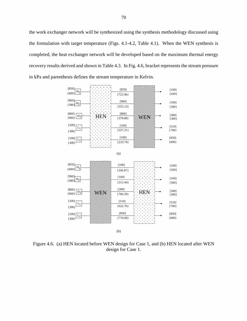
70
the work exchanger network will be synthesized using the synthesis methodology discussed using
the formulation with target temperature (Figs. 4.1-4.2, Table 4.1). When the WEN synthesis is
completed, the heat exchanger network will be developed based on the maximum thermal energy
recovery results derived and shown in Table 4.3. In Fig. 4.6, bracket represents the stream pressure
in kPa and parenthesis defines the stream temperature in Kelvin.
Figure 4.6. (a) HEN located before WEN design for Case 1, and (b) HEN located after WEN
design for Case 1.
[850]
[960][160]
[100]
[510]
[850]
[100]
[100]
[300][800]
1H
2H
3H
1L
2L
{600}
{580}
{960}
{700}
{600}
{430}
{300}
{300}
{300}
{300}
{722.96}
{555.13}
{378.80}
{337.21}
{233.74}
HEN WEN
[850]
[960]
[800]
[100]
[100]
[850]
[960][160]
[100]
[510]
[850]
[100]
[100]
[300][800]
1H
2H
3H
1L
2L
{600}
{580}
{960}
{700}
{600}
{430}
{300}
{300}
{300}
{300}
{356.87}
{313.44}
{760.29}
{622.76}
{770.09}
WEN HEN
[100]
[160]
[300]
[510]
[850]
(a)
(b)

71
Table 4.3. Energy recovery and operation cost comparison based on HEN location for Case 1
Statistic Placement of HEN
Before WEN After WEN
External compressors energy (kW) 1,431.98 1,628.13
External expanders energy (kW) 976.04 993.13
Mech. energy recovery by WEs (kW) 1,700.04 1,777.97
External heaters energy (kW) - -
External coolers energy (kW) 934.54 1,113.14
Thermal energy recovery by HEs (kW) 688.07 645.95
OPEX (k$/year) 1,382 1,572
Celec=0.12 $/kWh; Csteam=0.035 $/kWh; CCW=0.001 kWh;
Operating time=8000 h/year
For design problem with three high-pressure streams and two low-pressure streams, given
information from Table 4.2, and the design strategy of having the HEN before the WEN design,
the following matrices are calculated using the prediction methodology from Chapter 3 as inputs
to the flowcharts shown in Figs 4.1 and 4.2.
0 00 0
850 230510 230
230 170230 170
,,
,,
,,
P . (4.19)
The vector of mechanical energy will be provided by each individual high-pressure stream:
1,258.55
1,252.67
164.86
HW (4.20)
The vector of mechanical energy will be required by each individual low-pressure stream:
1,558.56
1,573.46
LW (4.21)
Matrix
W , which contains the information about the mechanical energy transferrable
between any pair of high-pressure and low-pressure streams:

72
00
36128183902
6818069266
β .,.
..
W (4.22)
and
γ
811.18
778.52
164.86
W . (4.23)
Considering NH=3, NL=2, Eqs. 4.19-4.23, and Fig. 4.1, WW is a 23 matrix as follows:
2313
2212
2111
L,HL,H
L,HL,H
L,HL,H
WW
WW
WW
W
WW
WW
WW
W , (4.24)
where the six elements will be derived as follows:
Evaluation of ,1 1H LW
W . Since 1γ
W (811.18 kW) is a positive value, we have:
kW692661111
β.WW
L,HL,HW
. (4.25)
Evaluation of ,1 2H LW
W . Since 1γ
W (811.18 kW) is a positive value, we have:
kW681802121
β.WW
L,HL,HW
. (4.26)
Evaluation of ,2 1H LW
W . Since 2γ
W (-778.52 kW) is a negative value, where its absolute value
is less than 12
βL,H
W (902.83 kW), both 12
βL,H
W and 22
βL,H
W (902.83 kW and 1,128.36 kW) are higher
than the absolute value of 2γ
W (-778.52 kW), and 12
βL,H
W (902.83 kW) will not be counted as the
highest value among 12
βL,H
W and 22
βL,H
W (902.83 kW and 1,128.36 kW), we have:
kW839021212
β.WW
L,HL,HW
. (4.27)

73
Evaluation of 22 L,H
WW . Since
2γW (-778.52 kW) is a negative value, where its absolute
value is less than 22
βL,H
W (1,128.36 kW), both 12
βL,H
W and 22
βL,H
W (902.83 kW and 1,128.36 kW) are
higher than the absolute value of 2γ
W (-778.52 kW), and 22
βL,H
W (1,128.36 kW) will be counted as
the highest value among 12
βL,H
W and 22
βL,H
W (902.83 kW and 1,128.36 kW), we have:
kW 843495277836128122222
γβ...,WWW
L,HL,HW
. (4.28)
Evaluation of 13 L,H
WW . Since
3γW (164.86 kW) is a positive value, we have:
, ,3 1 3 1
β0 kW
H L H LWW W . (4.29)
Evaluation of 23 L,H
WW . Since
3γW (164.86 kW) is a positive value, we have:
, ,3 2 3 2
β0 kW
H L H LWW W . (4.30)
Therefore, a complete matrix WW will be constructed using Eqs 4.25-4.30 as follows:
00
8634983902
6818069266
..
..
WW . (4.31)
Equation 4.31 shows the workload of each work exchanger unit between each individual
high-pressure and low-pressure stream where using splitting H1 and H2 will transfer mechanical
energy to L1 and L2 through four work exchangers. Now, MP which is a 23 matrix will be
constructed to identify the pressure interval in each individual low-pressure stream that the work
exchangers will be placed.

74
1 1 1 2
2 1 2 2
3 1 3 2
H ,L H ,L
H ,L H ,L
H ,L H ,L
M M
M M
M M
P P
P P
P P
MP , (4.32)
Derivation of two elements, 11,LH
MP and
22,LHM
P will be shown in the following. Calculation
of the other four elements can be performed in the same way.
a) Calculation of 11,LH
MP . This interval is derived from 11 L,HP . According to Eq. 4.4, the
upper-bound of both intervals will be the same and the lower-bound will be calculated using Eq.
T4.1-7 from Table 4.1. Note that based on the case study data provided, equation T4.1-7 is
modified to Eq. 4.34.
kPa23011
11
b
L,H
b
MPP
L,H
, (4.33)
and
1
1,1 1 1 1
1 1 1 1
11 1 11
1
170 kPa
CPL
R
PL
H L H , L
H , L H , L
PL
L
R
Cb
W Ma b
RM Mt t C
L L LP
W PP P
F C T P
(4.34)
Thus,
23017011
,P,LH
M (4.35)
b) Calculation of 22,LH
MP . This interval is derived from 22 L,HP . According to Eq. 4.4, the
upper-bound of both intervals will be the same and the lower-bound will be calculated using Eq.
T4.1-7 from Table 4.1. Note that based on the case study data provided, equation T4.1-7 is
modified to Eq. 4.37.
kPa85022
22
b
L,H
b
MPP
L,H
, (4.36)

75
and
2
2,2 2 2 2
2 2 2 2
22 2 22
1
610.40 kPa
CPL
R
PL
H L H , L
H , L H , L
PL
L
R
Cb
W Ma b
RM Mt t C
L L LP
W PP P
F C T P
(4.37)
Thus,
8504061011
,.P,LH
M (4.38)
c) Construction of a complete matrix MP . Using the same approach, we have calculated
the interval of the four other elements in matrix MP which are assembled as follows:
0000
85040610510230
230170230170
,,
,.,
,,
MP . (4.39)
According to Eq. 4.39, H1 requires splitting which will transfer 266.69 kW through a work
exchanger in 100, 850 pressure interval to L1 in the pressure interval of 170, 230 and 180.68
kW within the same pressure interval to L2 in the pressure interval of 170, 230 . H2 also requires
splitting and will transfer 902.83 kW through a work exchanger in 100, 850 pressure interval
to L1 in the pressure interval of 230, 510 and 349.84 kW within the same pressure interval to
L2 in the pressure interval of 610.40, 850 . At this stage, H3 will not transfer any mechanical
energy to any low-pressure stream.
Using Eqs. 4.6 and 4.7, vector 1C
W will be constructed as follows:

76
11
12
1,169.52 1,169.52
1,309.04 530.52
0
778.52
C
C
W
W
1CW
. (4.40)
Based on Eq. 4.40, one compressor will be placed in L2. The compressor location can be
defined as pressure interval of 230, 610.40 by comparing the pressure intervals from the second
column of matrices MP and P . Matrix 2C
W will be derived using Eqs. 4.8 and 4.9 as shown
below:
42264
04389
043091465731
521691575581
12
12
2
.
.
.,.,
.,.,
W
W
C
C
CW
. (4.41)
Comparing the pressure intervals in matrix P with the supply and target pressure of each
low-pressure stream from Table 4.2, two compressors will be placed. One of the compressors will
be placed in L1 within the pressure interval of 170, 230 with the workload of 389.04 kW and
the other one in L2 with the workload of 264.42 kW in the pressure interval of 170, 230 . In the
end, vector EW will be derived using Eqs. 4.10 and 4.11.
86164
0
18811
3
2
1
.
.
W
W
W
E
E
E
EW . (4.42)
Thus, two expanders will be placed. The first one will be in H1 through the splitting in the
pressure interval of 100, 850 with a workload of 811.18 kW, and the second one is in H3 within

77
the 300, 800 pressure interval with a workload of 164.86 kW. Figure 4.7a shows the flowsheet
developed through the WEN synthesis methodology. In Fig. 4.7a, there are three hot streams
(marked as HS1 – HS3) and two cold streams (marked as CS1 and CS2), which define a HEN
design problem. A synthesized HEN is shown in Fig. 4.7b. This network can recover 42.4% of
thermal energy from hot streams (688.07 kW out of 1,619.14 kW).
After the development of the work and heat exchanger network using the presented
methodology, the design can be modified by the instructions provided in the WEN design
modification using heat integration. According to Step I, the vector 1C
W contains only one
compressor ( 1C ) which is placed in the 230,610 pressure interval with the workload of 778.52
kW. This compressor can be matched with expander 1E by modifying the outlet temperature of
the expander using heat integration based on Step II (this is the type of design where the HEN
considered before the WEN). The adjusted outlet temperature for 1E will be 412 K which will
cause the expander 1E to transfer the exact amount of energy the compressor 1C requires.
Therefore, after replacing expander 1E and compressor 1C with a work exchanger ( 5W ), a heater
will be placed in the high-pressure stream so it will be heated to the target temperature (430 K).
Using this adjustment, the total mechanical energy recovery improved 31%, and external
compression utility consumption and expansion utility requirements decreased 54% and 17%,
respectively.
In conclusion, to reach the target temperature and pressure, three high-pressure streams and
two low pressure streams will go through a heat exchanger network (Fig. 4.7b) first and then a
work exchanger network (Fig. 4.8) in which the maximum amount of thermal and mechanical
energy will be recovered using this cost-effective design. The results are shown in Table 4.4.

78
Figure 4.7. Flowsheet of heat-integrated work exchange network for Case 1 :(a) work exchanger
network, (b) heat exchanger network.
[850]
[960][160]
[100]
[510]
[850]
[100]
[100]
(349.84)
[300][800]
[170][610](266.69)
(164.86)
(902.83)
(264.42)
(389.04)
(811.18)
1H
2H
3H
1L
2L
W4
W4
W3
W3
E1
C1
E2
C2
C3
{600}
{580}
{960}
{700}
{600}
{430}
{300}
{300}
{300}
{300}
W1
W2
W2
W1
{555}
{379}
{337}
{234}{295}(778.52) (180.68)
[230]
{490}
[230]{337}
CS1
HS1
HS2
HS3
CS2
{723}
{518}
[170]
{428}
<528.9>
1HS
2HS
3HS
1CS
2CS
{580}
{960}
{300}
{723}
{337}
{555}
{379}
{234}
{600}
{300}
HE1 HE2
HE1
{630}
<159.1>
HE2
<283.8>
<524.59>
<122.75>
4.30
4.91
2.09
4.30
4.30
CL1
CL2
CL3
{706}
Legend
Work exchanger
Expander
[ ] Pressure (kPa)
Heat transfer unit(s)
to be placed
W C Compressor
E
{ } Temperature (K) ( ) Work load (kW)
HE CLHeat exchanger Cooler
MC (kW/K)P < > Heat load (kW)
HeaterHET
(a)
(b)

79
Figure 4.8. Flowsheet of modified heat-integrated work exchange network for Case 1.
Table 4.4. Energy recovery analysis for Case 1
Design
Mech.
energy
exchange
(kW)
Thermal
energy
exchange
(kW)
External
compression
utility
(kW)
External
expansion
utility
(kW)
External
heating
utility
(kW)
External
cooling
utility
(kW)
Without
HEWEN - - 3,406.00 2,771.10 645.98 1,759.62
With
HEWEN 1,700.01 688.10 1,431.98 976.04 - 931.14
Modified
HEWN 2,478.53 688.10 653.46 164.86 47.93 931.14
Case 2. This design problem has been studied by Onishi et al. (2014) and Huang and
Karimi (2016). In both studies, a superstructure for work-heat exchanger network configuration
Legend
Work exchanger
Expander
[ ] Pressure (kPa)
Heat transfer unit(s)
to be placed
W C Compressor
E
{ } Temperature (K) ( ) Work load (kW)
HE CLHeat exchanger Cooler
MC (kW/K)P < > Heat load (kW)
HeaterHET
[850]
[960][160]
[100]
[510]
[850]
[100]
[100]
(349.84)
[300][800]
[170][610](266.69)
(164.86)
(902.83)
(264.42)
(389.04)
1H
2H
3H
1L
2L
W4
W4
W3
W3
E2
C2
C3
{600}
{580}
{960}
{700}
{600}
{430}
{300}
{300}
{300}
{300}
W1
W2
W2
W1
{555}
{379}
{337}
{234}{295}(778.52) (180.68)
{490}
[230]{337}
CS1
HS1
HS2
HS3
CS2
{723}
{518}
[170]
{428}
<47.93>
HETW5
W5
[230]
{412}

80
using single-shaft-turbine-compressor (SSTC) units was introduced and a mixed-integer nonlinear
programming (MINLP) model was conducted for identifying an optimal solution in terms of the
minimum total annualized cost. In Table 4.5, data for this synthesis problem is summarized.
Table 4.5. Process stream data for Case 2
Stream
No.
Supply
pressure
(Ps, kPa)
Target
pressure
(Pt, kPa)
Flowrate
(kg/s)
Source
temperature
(Ts, K)
Target
temperature
(Tt, K)
Heat
capacity
(CP, kJ/kg.k)
H1 900 100 15 350 350 2.454
H2 850 150 15 350 350 0.982
H3 700 200 15 400 400 1.432
L1 100 700 18 390 390 1.432
L2 100 900 15 420 420 2.454
Step a. Assume HEN before WEN. Considering the heat exchanger network before the
work exchanger design means that streams will go through a process of heating or cooling before
entering the work exchanging stage. The first step is to use the specified outlet temperatures and
calculate the temperature (H
iT and L
iT ) each stream will reach after exiting the HEN. Knowing
the inlet temperature of each stream, stream data will be defined for the HEN problem. In the
following, using Eqs. 4.12 and 4.13, the outlet temperature after the HEN design is shown for
streams HP1 and LP1.
K70655
900
100
350
41
40
1
1
1
11
.
P
P
TT
.
.
k
K
s
H
t
H
t
HH
i
(4.43)
and

81
K67223
100
700
390
41
40
1
1
1
11
.
P
P
TT
.
.
k
k
s
L
t
L
t
LL
i
(4.44)
where k is the heat capacity ratio (adiabatic exponent).
With the same structure, all the temperatures are specified and the HEN design problem is
defined as shown in Fig. 4.9a. As discussed and shown in Fig. 4.3, after calculating the H
iT and
L
iT for the streams, the maximum amount of mechanical energy that can be recovered for the
problem design should be predicted using the methodology presented in Chapter 3. The three
high-pressure streams will provide 18,257.91 kW mechanical energy through depressurization
where two low-pressure streams require 11,495.23 kW energy for pressurization. Using the
prediction methodology 8,846.94 kW of mechanical energy of the high-pressure streams can be
transferred to the low-pressure streams which accounts for 48.46% of the total energy of the high-
pressure streams and 76.96% of the energy of the low-pressure streams required for pressurization.
The next stage is to predict the maximum amount of thermal energy that can be recovered using
the pinch analysis. Similar to the prediction stage, the detailed calculations for pinch analysis (i.e.,
temperature interval and cascade diagram) are not shown here. For this design problem as shown
in Fig. 4.9a, there are three cold streams (H1, H2, and H3) which require 18,257.91 kW energy to
be heated and two hot streams (L1 and L2) with 11,495.23 kW energy. The results from pinch
analysis show that about 2,908.2 kW energy that cold streams require can be provided by hot
streams which accounts for 25% of the energy of the hot streams and 16% of the energy of the
cold streams.

82
Operating cost for the current design considering the cost of utilities such as electricity,
steam and cooling water is calculated using Eq. 4.14.
Step b. Assume HEN after WEN. For this step, the design problem will be defined as
shown in Fig. 4.9b where output temperatures have been calculated using Eqs. 4.15 and 4.16. The
prediction stage will be conducted based on the formula for having the HEN after the WEN design
where three high-pressure streams will provide 10,606.49 kW of mechanical energy through
depressurization and two low-pressure streams require 20,979.15 kW of the energy for
pressurization. Using the prediction methodology 6,006.59 kW of mechanical energy of the high-
pressure streams can be transferred to the low-pressure streams which accounts for 56.63% of the
total energy of the high-pressure streams and 28.63% of the energy of the low-pressure streams
required for pressurization. The next stage is to predict the maximum amount of thermal energy
that can be recovered using the pinch analysis. Similar to the prediction stage, the detailed
calculations for pinch analysis (i.e., temperature interval and cascade diagram) are not shown here.
For this design problem as shown in Fig 4.9b, there are three cold streams (H1, H2, and H3) which
require 10,606.54 kW energy to be heated and two hot streams (L1 and L2) with 20,979.3 kW
energy. The results from pinch analysis show that the total amount of energy that cold streams
require can be provided by hot streams which accounts for 50.56% of the energy of the hot streams
and 100% of the energy of the cold streams.
The results from both methods are summarized in Table 4.6. Comparing the operating cost
of the two designs shows that the heat exchanger network before the work exchanger design would
be more cost-effective in terms of operating cost. For this reason, we will locate the heat exchanger
network first (Fig. 4.4a and 4.9a) to heat and cool down the high-pressure and low-pressure streams
and then design a work exchanger network to reach the target pressure and temperature defined

83
for this case study based on Table 4.5. After the decision on the location of the HEN is made, the
work exchanger network will be synthesized using the synthesis methodology (Figs. 4.1-4.2) and
the formulation considering the target temperature (Table 4.1). The heat exchanger network will
be also developed based on the maximum thermal energy recovery results shown in Table 4.6.
Table 4.6. Energy recovery and operation cost comparison based on HEN location for Case 2
Statistic Placement of HEN
Before WEN After WEN
External compressors energy (kW) 2,648.29 14,972.56
External expanders energy (kW) 9,410.97 4,599.90
Mech. energy recovery by WEs (kW) 8,846.94 6,006.59
External heaters energy (kW) 15,349.71 -
External coolers energy (kW) 8,587.03 10,372.76
Thermal energy recovery by HEs (kW) 2,908.20 10,606.54
OPEX (k$/year) 6,909 14,457
Celec=0.12 $/kWh; Csteam=0.035 $/kWh; CCW=0.001 kWh;
Operating time=8000 h/year

84
Figure 4.9. (a) HEN located before WEN design for Case 2, and (b) HEN located after WEN
design for Case 2.
For design problem with three high-pressure streams and two low-pressure streams, given
information from Table 4.5 and the design strategy of having the HEN before the WEN design,
the following matrices are calculated using the prediction methodology as inputs to the flowcharts
shown in Figs 4.1 and 4.2.
0 00 0
0 00 0
308 170007 170
,,
,,
,,
P . (4.45)
[900]
[850][150]
[100]
[700]
[900]
[100]
[100]
[200][700]
1H
2H
3H
1L
2L
{350}
{350}
{400}
{390}
{420}
{350}
{350}
{400}
{390}
{420}
{655.71}
{574.52}
{572.15}
{223.67}
{224.19}
HEN WEN
[900]
[850]
[700]
[100]
[100]
[900]
[850][150]
[100]
[700]
[900]
[100]
[100]
[200][700]
1H
2H
3H
1L
2L
{350}
{350}
{400}
{390}
{420}
{350}
{350}
{400}
{390}
{420}
{186.82}
{213.22}
{279.65}
{680.02}
{786.85}
WEN HEN
[100]
[150]
[200]
[700]
[900]
(a)
(b)

85
The vector of mechanical energy will be provided by each individual high-pressure stream:
11,253.02
3,307.17
3,697.73
HW
. (4.46)
The vector of mechanical energy will be required by each individual low-pressure stream:
7,207.91
4,287.32LW . (4.47)
Matrix
W , which contains the information about the mechanical energy transferrable
between any pair of high-pressure and low-pressure streams.
00
00
435035513433
β
.,.,
W , (4.48)
and
γ
2,406.08
3,307.17
3,697.73
W . (4.49)
Considering NH=3, NL=2, Eqs. 4.45-4.49, and Fig. 4.1, WW is a 23 matrix as follows:
2313
2212
2111
L,HL,H
L,HL,H
L,HL,H
WW
WW
WW
W
WW
WW
WW
W , (4.50)
The derivation of all the six elements is shown below:
Evaluation of 11 L,H
WW . Since
1γW (2,406.08 kW) is a positive value, we have:
kW5134331111
β.,WW
L,HL,HW
. (4.51)

86
Evaluation of 21 L,H
WW . Since
1γW (2,406.08 kW) is a positive value, we have:
kW4350352121
β.,WW
L,HL,HW
. (4.52)
Evaluation of 12 L,H
WW . Since
2γW (3,307.17 kW) is a positive value, we have:
kW01212
β
L,HL,H
WWW
. (4.53)
Evaluation of 22 L,H
WW . Since
2γW (3,307.17 kW) is a positive value, we have:
kW 02222
β
L,HL,H
WWW
. (4.54)
Evaluation of 13 L,H
WW . Since
3γW (3,697.73 kW) is a positive value, we have:
kW01313
β
L,HL,H
WWW
. (4.55)
Evaluation of 23 L,H
WW . Since
3γW (3,697.73 kW) is a positive value, we have:
kW02323
β
L,HL,H
WWW
. (4.56)
Therefore, the complete matrix WW will be constructed using Eqs. 4.51-4.56 as follows:
00
00
435035513433 .,.,
WW . (4.57)
Equation 4.57 shows the workload of each work exchanger unit between each individual
high-pressure and low-pressure stream. Using splitting, H1 will transfer mechanical energy to L1
and L2 through two work exchangers. MP which is a 23 matrix will be constructed to identify
the pressure interval in each individual low-pressure stream that the work exchangers will be
placed in.

87
2313
2212
2111
,LH,LH
,LH,LH
,LH,LH
MM
MM
MM
PP
PP
PP
MP , (4.58)
Derivation of the two elements, 1 1H ,LM
P and 2 2H ,LM
P will be shown in the following.
Calculation of the other four elements can be performed in the same way.
a) Calculation of 1 1H ,LM
P . This interval is derived from 11 L,HP . According to Eq. 4.4, the
upper-bound of both intervals will be the same and the lower-bound will be calculated using Eq.
T4.1-7 from Table 4.1. Note that based on the case study data provided, equation T4.1-7 is
modified to Eq. 4.60.
kPa70011
11
b
L,H
b
MPP
L,H
, (4.59)
and
1
,1 1 1 1
1 1 1 1
1 1 11
1
11
170 kPa
k
k
H L H , L
H , L H , L
L
k
kb
W Ma b
kM Mt t k
L L LP
W PP P
F C T P
(4.60)
Thus,
70017011
,P,LH
M (4.61)
b) Calculation of 2 2H ,LM
P . This interval is derived from 22 L,HP . According to Eq. 4.4, the
upper-bound of both intervals will be the same and the lower-bound will be calculated using Eq.
T4.1-7 from Table 4.1. Note that based on the case study data provided, equation T4.1-7 is
modified to Eq. 4.63.
kPa83022
22
b
L,H
b
MPP
L,H
, (4.62)

88
and
1
,2 2 2 2
2 2 2 2
2 2 22
1
11
170 kPa
k
k
H L H , L
H , L H , L
L
k
kb
W Ma b
kM Mt t k
L L LP
W PP P
F C T P
(4.63)
Thus,
83017011
,P,LH
M (4.64)
c) Construction of a complete matrix MP . Using the same approach, we have calculated
the values of the four other elements in matrix MP . All these values are assembled as follows:
0000
0000
830170700170
,,
,,
,,
MP . (4.65)
According to Eq. 4.65, H1 requires splitting which will transfer 3,343.51 kW through a
work exchanger in the 100,900 pressure interval to L1 in the pressure interval of 170,700 and
5,503.43 kW within the same pressure interval to L2 in the pressure interval of 170,830 . H2 and
H3 will not transfer any mechanical energy to any low-pressure stream.
Using Eqs. 4.6 and 4.7, vector 1C
W will be constructed as follows:
0
0
435035435035
513433513433
21
11
.,.,
.,.,
W
W
C
C
1CW
. (4.66)
Matrix 2C
W will be derived using Eqs. 4.8 and 4.9 as shown below:

89
487041
81943
435035912077
513433322874
12
12
2
.,
.
.,.,
.,.,
W
W
C
C
CW
. (4.67)
According to Eqs. 4.66 and 4.67, there will be only two compressors which will be placed
by comparing the pressure intervals in matrix P with the supply and target pressures of each low-
pressure stream from Table 4.5. The comparison will end up with placing three compressors, the
first one in L1 within the pressure interval of 100,170 with the workload of 943.81 kW, the
second and third ones in L2 with the total energy of 1,443.87 kW in the pressure intervals of
100,170 and 830,900 with workloads of 1,350.93 kW and 353.55 kW, respectively. In the
end, vector EW will be derived using Eqs. 4.10 and 4.11.
736973
173073
084062
3
2
1
.,
.,
.,
W
W
W
E
E
E
EW . (4.68)
Thus, three expanders will be placed. The first one will be in H1 through the splitting in
the pressure interval of 100,900 with the workload of 2,406.08 kW, the second one is in H2
within the 150,850 pressure interval with the workload of 3,307.17 kW, and the third one is in
H3 within the 200,700 pressure interval with the workload of 3,697.73 kW. Figure 4.10a shows
the flowsheet developed using the WEN synthesis methodology. In Fig. 4.10(a), there are three
hot streams (marked as HS1 – HS3) and two cold streams (marked as CS1 and CS2), which define
a HEN design problem. A synthesized HEN is shown in Fig. 4.10(b). This network can recover
25% of the thermal energy from the hot streams (8,587.03 kW out of 11,495.23 kW).

90
After the development of the work and heat exchanger networks using the presented
methodologies, the design will be analyzed for any possibility of additional modification by heat
integration. According to Eq. 4.66, there will not be any compressor placed using vector1C
W .
Thus, there will not be any low-pressure stream in the thermodynamic feasibility pressure interval
to be able to receive energy from the high-pressure streams by adjusting the temperature.
For this case study, we have conducted a cost analysis to estimate the Total Annualized
Cost (TAC) including Capital Cost (CAPEX) and Operating Cost (OPEX). For a reasonable
comparison of the final results with Huang and Karimi (2016) and Onishi et al. (2014), we have
used the exact same assumptions for the cost calculation such as formulation, equipment cost
coefficient and fixed cost, and utility cost. As mentioned earlier, those studies have used SSTC
units for the mechanical energy recovery. Therefore, for the capital cost estimation of work
exchangers in our design, we have used the base cost formula discussed in Section 4.3 and Fig.
4.5. The capital cost of external expanders ( ECAPEX ) is computed using Eq. 4.69.
U
E E ECAPEX FC FC F (4.69)
where U
EFC is the external expander fixed cost and is assumed to be 200 k$/year, EFC is the cost
coefficient and is equal to 1 k$/year, and F is the flowrate of stream flows through the expander.
The capital cost of external compressors ( CCAPEX ) is computed using Eq. 4.70.
U
C C CCAPEX FC FC F (4.70)
where U
CFC is the external compressor fixed cost and is assumed to be 250 k$/year, CFC is the
cost coefficient and is equal to 1 k$/year, and F is the flowrate of stream flows through the

91
compressor. The capital costs of heat exchangers, heaters, and coolers ( HECAPEX ) are computed
using Eq. 4.71.
δ
HE HCAPEX FC C A (4.71)
where HFC is the heat exchanger fixed cost and is assumed to be 3 k$/year, C is the cost
coefficient and is equal to 0.03 k$/year, A is the heat exchanger area, and δ is the exponent for
area cost of the HE and is equal to 1. The capital cost of the work exchanger ( WECAPEX ) will be
computed as follows:
βαWECAPEX S (4.72)
where S is the volume of one vessel and cost parameters assuming stainless steel, the pressure
tolerance of 1,034 MPa for a vessel and 5 MPa for valves, are 995.78 and 0.36 for α and β ,
respectively.
For operating cost estimation, Eq. 4.14 and the assumptions for the utility cost from Table
4.6 are used. The cost estimation of all the units for case 2 shown in Fig. 4.10 is summarized in
Table 4.7. The Total Annualized Cost (TAC) for this case study using the heat-integrated work
exchange synthesis design using work exchangers will be $9,666,994. In Table 4.8, the results for
the cost-effective design of the heat exchanger network (Fig. 4.10b) combined with a work
exchanger network (Fig. 4.10a) that can recover a significant amount of thermal and mechanical
energy are summarized and compared with the Onishi et al. (2014) and Huang and Karimi (2016)
work.

92
Figure 4.10. Flowsheet of heat-integrated work exchange network for Case 2: (a) work
exchanger network, and (b) heat exchanger network.
[170](3,343.15)
(3,307.17)
(1,350.93)
(943.81)
(2,406.08)
1H
2H
3H
1L
2L
W2
W2
W1
W1
E1
E3
C1
C2{261}(5,503.43)
CS1
CS2
CS3
HS2
HS1[170]
{260}
[900]
[850]
[700]
{350}
{350}
{400}
[700]
[900]
{390}
{420}
[150]
[100]
[200]
{350}
{350}
{400}
[100]
[100]
{390}
{420}
{656}
{575}
{572}
{224}
{224}
E2
(3,697.73)
{410}
[830]C3
(353.55)
<2,392.65>
1HS
2HS
2CS
3CS
{420}
{390}
{656}
{575}
{572}
{223.67}
{224.19}
{350}
{350}
{400}
HE1
HE2
HE1
{370}
<515.55>
HE2
<4,815.26>
36.81
25.77
36.81
14.73
21.48
CL1
CL2
1 1CS
{355}
{385}
<3,771.77>HET
3HET
<3,697.73>
<8,860.37>{415}
2HET
<2,791.62>
Legend
Work exchanger
Expander
[ ] Pressure (kPa)
Heat transfer unit(s)
to be placed
W C Compressor
E
{ } Temperature (K) ( ) Work load (kW)
HE CLHeat exchanger Cooler
MC (kW/K)P < > Heat load (kW)
HeaterHET
(a)
(b)

93
Table 4.7. CAPEX and OPEX of units in Case 2
Equipment Size Factor CAPEX ($/year) OPEX($/year)
HE1 A=9,570 m2 290,118 -
HE2 A=952 m2 31,554 -
HET1 A=734 m2 118,226 2,480,904
HET2 A=182 m2 76,816 781,654
HET3 A=245 m2 25,021 1,035,364
CL1 A=3,841 m2 8,469 38,522
CL2 A=2,461 m2 10,351 30,174
C1 F= 25.77 kW/k 275,776 906,058
C2 F= 36.81 kW/k 286,810 339,408
C3 F= 36.81 kW/k 286,810 1,296,893
E1 F= 7.87 kW/k 207,871 -
E2 F= 14.73 kW/k 214,730 -
E3 F= 21.48 kW/k 221,480 -
W1 S= 20 L (10
vessels used) 351,993 -
W2 S= 20 L (10
vessels used) 351,993 -
Total 2,758,018 6,908,976
To size the heat exchangers, heaters and cooler, the formulation to compute the area and
overall heat transfer coefficient is given by the Huang and Karimi (2016) study and can be found
in their publication. Using the formulation presented, the details for the area calculation will be
straightforward so they will not be discussed here. The size factor for compressors and expanders
is the multiplication of flowrate and heat capacity given for each stream using Table 4.5 and Fig.
4.10a. To size the work exchangers, the volume of each vessel is required. However, to estimate
the volume, the cycle time of the energy recovery in the device and volumetric flowrate of the
stream flows through the unit are required. Cycle time of work exchangers dealing with gas phases
will be addressed in Chapter 5. However, due to several challenges in estimation of cycle time, at
this stage, we will make assumptions based on the worst case scenario. In addition, the volumetric
flowrate for the streams is not provided and streams components are not available. Therefore, the
mass flowrate given cannot be converted to a volumetric flowrate. It is expected that the streams

94
have a high volumetric flowrate based on the given mass flowrate and considering the low dense
gases flowing through. Therefore, we have considered each vessel of the work exchanger with
volume of 20 L which is among the largest displacement vessels were found in commercial scale;
and assumed 10 vessels in each unit. Therefore, the cost that will be calculated from Eq. 4.72 for
a vessel of 20 L will be multiplied by 10.
Table 4.8. Performance comparison of HIWENs by different methods for Case 2
Design This
Work
Onishi et al.
(2014)
Huang and Karimi
(2016)
Mech. energy exchange (kW) 8,847 10,474 11,579
Thermal energy exchange (kW) 2,908 8,794 15,920
Compression utility (kW) 2,648 8,840 7,734
Expansion utility (kW) 9,411 - -
Heating utility (kW) 15,349 1,680 5,276
Cooling utility (kW) 8,587 10,520 13,010
No. of WEs 2
3 SSTC
Compressors+3 SSTC
Turbines
3 SSTC
Compressors+3 SSTC
Turbines
No. of HEs 2 8 6
No. of HET and CL 5 5 9
No. of compressors 3 2 1
No. of expanders/valves 3 1 -
CAPEX (k$/yr) 2,758 - 1,180
OPEX (k$/yr) 6,909 - 9,006
TAC (k$/yr) 9,667 10,502 10,187
In general, our design is less complicated with lower compression, heating, and cooling
utility consumption. Note that due to pressure and temperature correlations, the assumptions made
regarding the heat integration will impact the total amount of energy high-pressure streams can
provide during the depressurization, and low-pressure streams required for pressurization.
Therefore, total mechanical energy recovery will not be necessarily the best parameter for
comparison at this stage. The capital cost for our design is higher than the Huang and Karimi
(2016) superstructure design which can be explained as the result of more compressors and
expanders, in addition to the cost of work exchangers which is still in the stage of preliminary

95
estimation. The total capital cost of SSTC compressors and SSTC turbines in the Huang and
Karimi (2016) study is 431,382 $/year but for the work exchangers in our design is 703,986 $/year.
As mentioned earlier, the unit sizing and cost estimation for the work exchanger has been
performed under several assumptions considering the worst case scenario. Therefore, we are
expecting the cost to decrease as more details are available regarding the design of work
exchangers. The operating cost in our design is significantly lower than Huang and Karimi (2016)
design as a result of lower utility consumption. The total Annualized Cost (TAC) of our design is
about 5% lower than that for the Huang and Karimi (2016) superstructure. Even though we have
not performed an optimization study for TAC minimization, our final solution is more cost
effective than the previous studies. In addition, the solution is much simpler, and easier to conduct.
This shows the efficacy of the presented heat integrated work exchange network synthesis
methodology.
4.5 Summary
In this chapter, we proposed a heat-integrated work exchanger network synthesis
methodology to develop a cost-effective network for mechancial and thermal energy recovery. It
is preferred to determine the location of the HEN prior to completion of the final WEN network.
However, in some studies, the HEN has been always located before the WEN design when low-
pressure streams are considered as hot and high-pressure streams as cold streams. The goal is to
increase the amount of energy provided by expansion and decrease the amount of energy required
for compression. We believe that to be able to have a general methodology for heat and work
exchanger network synthesis, the location of heat integration should be announced based on the
option with the least operating cost which represents the design with lowest energy-intensive

96
utility. As shown in case studies, using the presented methodology we are able to derive less
complicated designs with better performance in terms of utility consumption and operating cost.
Capital cost estimation was conducted for the first time in a design in which direct work
exchangers are integrated. The cost estimation for the work exchanger can be considered as an
early investigation in the economic analysis of the direct type of mechanical energy recovery
devices known as work exchangers. However, it still requires further studies while the device is
being modified to be used in chemical processes dealing with gas phase streams.
The heat-integrated work exchange network synthesis methodology can be also developed
in the future for the design of more realistic flowsheets in terms of assumptions made through the
flowsheet construction, temperatures computed using the heat-integration technique before or after
the WEN, unit operation size and capacity, and the possibile phase change through the
compression/expansion. Development of a framework for a simultaneous recovery of thermal and
mechancial energy without initial assumptions of one network before or after the other, can be
defined as a future study.

97
CHAPTER 5 MODELING AND SIMULATION OF A PISTON-TYPE WORK
EXCHANGER FOR MECHANICAL ENERGY RECOVERY
The significance of energy efficiency improvement in chemical processes has led to
increasing research opportunities for innovative process integration technologies. Recovery of
mechanical energy through work exchanger network synthesis is a type of process integration that
has been recently drawn a lot of attention. Direct (one-step) Work Exchangers (WEs) can be
considered as a type of process unit for mechanical energy recovery in chemical plants. The type
of device was first introduced for reverse osmosis (Cheng et al., 1967; Cheng and Cheng, 1970).
Dual Work Exchange Energy Recovery Device (DWEER) is a piston-type WE that has been
widely used for seawater reverse osmosis (RO) desalination, which is one of the most efficient
energy recovery systems developed to date. However, this type of unit cannot be directly used for
the pressurization/depressurization of process streams in the gas phase in chemical plants.
5.1 Objectives and Significance
The work exchanger dealing with gas phase streams will have a different behavior. The
safety issues regarding leakage and mixing losses will increase when dealing with gas streams.
These will also impact the efficiency of the system, the maintenance cost, and the operating cost.
DWEERs are always running with the same materials (i.e., brine and seawater) which are non-
hazardous and non-flammable. On the other hand, the work exchangers for mechanical energy
recovery through WEN will be operated using different types of materials and under various
operating conditions such as temperature, pressure, and physical properties. Therefore, deep
investigation through work exchanger component parts, future unit modification to ensure the
safety, a possible improvement on unit efficiency, and compatiblity of the unit with different types
of material would be required.

98
To show the feasibility of using a direct work exchanger as a device for mechanical energy
recovery, we need to have better insight on the device performance. Computational modeling and
simulation of the device could be the first stage prior to manufacturing of the unit in the pilot and
industrial scales. To start the modeling of the work exchangers, the first step is to collect sufficient
information about the device. A detailed description has been provided by Cheng and Fan (1968)
regarding the size, structure, and work exchanger operation. In Chapter 2, the description of
pressurization and depressurization steps provided by Cheng et al. (1967) has been discussed.
Based on the description provided for the desalination application, the device contains two
displacement vessels, check valves, control valves, and three additional pumps. The pumps will
be used for maintaining the inlet pressure of the low-pressure stream higher than the outlet pressure
of the high-pressure stream, maintaining the inlet pressure of the high-pressure stream higher than
the outlet pressure of the low-pressure stream, and pressurizing the excess part of the feed. To
manufacture the unit, commercially available component parts were used with some modifications.
Figure 5.1 shows a schematic of one piston-type work exchanger provided by Cheng and Fan
(1968).
The unit contains two 2 gallon floating piston-type accumulators as the two displacement
vessels (O1 and O2), four hydraulic check valves (v1, v2, v3, and v4), and two 2-way control valves
or one 4-way hydraulic valve as the valves for v5, v6, v7, and v8. The details for other component
parts such as pumps, flowmeters, the programming timer, and pipe fittings have not been discussed
here since they will not impact the simulation and modeling setup at this stage. However, those
parts should be studied at the time of manufacturing of the unit for gas phase streams.

99
Figure 5.1. Schematic illustration of a piston-type work exchanger (Cheng and Fan, 1968).
The component parts were connected by 3/4", schedule-160 steel pipes in assembling the
unit. The unit was operable up to 102 atm (1,500 psig) and delivered 2.45 m3/hr (9 gpm). Water
was used as the working fluid, and the cycle time for 2.45 m3/hr (9 gpm) capacity was adjusted to
20 seconds. The maximum displacement of the piston per stroke was 6.81 L (1.8 gallons) but at
each half cycle, 5.6 L (1.5 gallons) entered the vessel. To solve the problem of non-steady flow

100
because of the valve shifting, they installed an accumulator. It was mentioned that each of the
flowrates multiplied by half of the time cycle time should not exceed the volume filled by the
piston in a stroke, and the inlet rate for each side should be adjusted to the same value. Also, it
was discussed that the capacity of the unit can be increased to 5.45 m3/hr (20 gpm) by changing
pipe fittings, valves, and pipe size to 1".
Dual Work Exchanger Energy Recovery (DWEER) which is being manufactured at the
industrial scale by Flowserve consists of two pressure vessels, four check valves, and one patented
LinX control valve. The single unit can process up to 75 bar and 350 m3/hr or 1.4 mgd and to
achieve higher volume, the manufacturer suggested placing multiple units in parallel. This device
is being used in Reverse Osmosis (RO) plants around the world such as in Spain, Australia, Dubai,
and Singapore. Recovering up to 98% of the energy in the brine stream, operational flexibility,
robust design, high availability, low maintenance costs, and low mixing and leakage rates have
been mentioned as some of the main features (Flowserve, 2018).
In the following, the piston-type work exchanger has been simulated using customizing
operation models in Aspen Plus and computational fluid dynamic modeling with Ansys Fluent.
The main objective is to analyze the performance of the unit which is being used in desalination
processes when dealing with the gas phase and different type of materials.
5.2 Modeling and Simulation of Work Exchanger Systems Using Aspen Plus
Simulation of unit operation is a tool to evaluate the process configuration and help to
understand the parameters which impact the process specifications. The piston-type work
exchanger is a new unit operation which can be used in process systems for mechanical energy
recovery and is not available as a built-in unit operation similar to heat exchangers in any process

101
simulation software. However, Aspen Plus as one of the promising process simulators in the
chemical industry allows users to add customized modules using Aspen Custom Modeler.
Aspen Custom Modeler in combination with Microsoft Excel and Visual Basic can be used
to simulate a unit operation and include the customized unit into the Aspen Plus model library.
This will enable users to model the particular unit operation, build the model library and export it
into Aspen Plus for the process simulation. In the following, the simulation procedure is discussed.
5.2.1 Construction of work exchanger module with Aspen Plus
In a piston-type work exchanger, the high-pressure and low-pressure streams will be each
on one side of the piston without having any contact. Due to opening and closing of the valves
and movement of the piston, the pressure of each stream will change. The temperature may also
differ under non-isothermal conditions. The module includes two inlet feeds and two outlet
streams, one of each for the high-pressure stream and the low-pressure stream.
Figure 5.2. Schematic representation of a work exchanger module.
Figure 5.2 which shows the work exchanger module is a general representation of the unit
which means that multiple vessels and valves for inlet and outlet streams will be included in the
presented module. However, similar to other unit operations in Aspen Plus, the model formulation
impacts how the outlet stream specification will be calculated using the given inlet stream
information and additional parameters. In the work exchanger module, the high-pressure stream
will be depressurized (expanded) and the low-pressure stream will be pressurized (compressed).
Therefore, the following equations will be used in the simulation model for the unit operated with
streams assumed to behave as ideal gas.
in in
L L, P ,Tin
LF
L L, P ,Tout out out
LF
in in, P ,Tin
H H HF
, P ,Tout out out
H H HF

102
There will not be any reaction, and mixing or leakage through the process. Then, Eqs. 5.1-
5.4 represent the model mass balance. The mass balance for the compartment containing the high-
pressure stream will be as follows:
in out
H HF F , (5.1)
and
in in out out
H H H HF C F C . (5.2)
For the compartment containing the low-pressure stream:
in out
L LF F , (5.3)
and
in in out out
L L L LF C F C . (5.4)
where F represents the mass flowrate and C composition.
Based on the system degree of freedom, the outlet pressure of the high-pressure or low-
pressure stream should be given. Therefore, the outlet pressure of the high-pressure stream will
be defined through one of the three conditions shown in Eq. 5.5.
; User identified
; User identified IsothermalCondition
exp
1
out out
H H
inoutH
L
out
H in
H
in
H in in
H p H
P P
PP
WP
n RT
WP
F C T
1
; User identified AdiabaticCondition
m
mout
LP
. (5.5)

103
In a similar way, the outlet pressure of the low-pressure stream will be defined using Eq.
5.6.
; User identified
; User identified IsothermalConditioninL
out out
L L
W
n RTout in out
L L H
in
L in in
L p L
P P
P P e P
WP
F C T
1
1 ; User identified AdiabaticCondition
m
mout
HP
. (5.6)
where W represents the mechanical energy exchanged between the high-pressure and low-
pressure streams through the process. Table 2.1 can be used as the formula directory. n represents
the molar rate. pC is the heat capacity, R is the gas constant, and m is the adiabatic (polytropic)
exponent. The outlet temperature for either the high-pressure or low-pressure stream will be
calculated using Eq. 5.7.
1
; IsothermalCondition
; AdiabaticCondition
in
moutout m
in
in
T
TP
TP
. (5.7)
5.2.2 Simulation Procedures
According to the modeling described in the previous section, the simulation has been
completed. As mentioned earlier, in Aspen Plus users can create customized modules by
modifying the available FORTRAN interface subroutine and the Excel model (Aspen Technology
Inc., 2013). The simulation steps have been summarized in the following.
Setting up the model in Aspen Plus. After creating an Aspen Plus blank simulation, from
User models, User2 icon PLUG will be selected as the model with two inlets and two outlet
streams.

104
Setting up the Excel model. An Excel template available in the Aspen Plus user library
will be customized based on our unit operation model. The Excel file contains several sheets for
modifying the model integer and real parameters, input information and required formula for
calculation of the model output streams. The gas constant and mechanical energy exchanged
between high-pressure and low-pressure streams (W ) will be considered as the real parameter.
There will not be any integer parameter for this model. To solve the model, additional inputs are
required according to the degree of freedom of the system. For this model, one of the outlet
pressures is the additional information that needs to be provided by the user. Using the outlet
pressure, W will be calculated by the system as discussed in section 5.2.1. The screenshots of the
Excel model are highlighted in Fig. 5.3.
Revising the user subroutine. The unit operation model subroutine should be customized
to pass the input data such as feed streams from the Aspen Plus to Excel and pass the calculated
output data from the Excel to Aspen Plus. Similar to the Excel model, a template code for the
User 2 model is available in the Aspen Plus library to be modified for our model. The User 2 user
subroutine which has been analyzed and shown in Aspen Plus User Models and Getting Started
Customizing Unit Operation Models (2012, 2013) will not be discussed in detail here as the
changes are minor. Appendix C contains the customized User 2 unit operation model subroutine
for Excel models from Aspen Plus Getting Started Customizing Unit Operation Models (2013) for
the work exchanger model.

105
Figure 5.3. Summary of the Excel model set up.
The next steps include compiling and linking the subroutine to Aspen Plus, creating a
shared library for the model, customizing the Aspen Plus model library, and editing the custom
model schematic based on the work exchanger (Aspen Technology Inc., 2013). These steps will
be similar for all models so we will not discuss them here.
5.2.3 Simulation Results
The simulation has been run using Aspen Plus V8.4, Visual Studio 2015, and Microsoft
Excel 2013 in a computer operating with Microsoft Windows 7. At this stage, as long as the work
exchanger model library is available in the Aspen Plus working folder, we will be able to add the
work exchanger unit from the unit operations palette.
One of them is defined
by user.
One of them is calculated
using Table 2.1.
=calculated W(HP) or
W(LP) from sheet1
Entered by user
in Aspen Plus
Defined by
Aspen Plus
Eq. (5.2)Eq. (5.1)
Eq. (5.4)Eq. (5.3)
Eq. (5.7) Eq. (5.7)Eq. (5.5) Eq. (5.6)
Defined by Aspen
Plus

106
Figure 5.4. Work exchanger unit in the Aspen Plus environment.
Case 1. For a case study of a high-pressure stream that enters the work exchanger at 2,000
kPa and 525 k with a molar flowrate of 23.19 mol/s with ammonia as the only component, and a
low-pressure stream that enters the unit at 220 kPa and 330 k with a molar flowrate of 82.54 mol/s
and ammonia as the component, the objective is to depressurize the high-pressure stream to 150
kPa. The case study is under the isothermal condition, with the ideal gas assumption and
considering 100% efficiency of the unit. The property method is Peng-Robinson. Figure 5.5
shows the inlet information for the streams and the specified outlet for the high-pressure stream in
Aspen Plus.
LPIN
LPOUT
HPIN
HPOUT
WE

107
Figure 5.5. Inlet data required to run the simulation.
The simulation will be run and the outlet stream specification will be calculated by passing
the inlet data from Aspen Plus to Excel for calculation through the FORTRAN user subroutine and
the results will be passed back to Aspen Plus. Figure 5.6 shows the outlet stream’s data and the
amount of work that will be exchanged through the work exchanger.

108
Figure 5.6. Final streams and unit capacity results for Case 1.
Case 2. To show the feasibility of simulating the customized work exchanger model with
other unit operations, we have simulated the case study 1 from Chapter 3 (Liu et al., 2014). The
same assumptions have been made through the simulation except there will be temperature change
for the streams passing through the external compressors and expanders since these unit operations
can be only simulated in Aspen Plus under non-isothermal conditions. Figure 5.7 represents the
work exchange network designed in Chapter 3 (Figure 3.3a). We refer to section 3.2.2 for details
on network design derivation.

109
Figure 5.7. Simulated work exchanger network in Aspen Plus for Case 2.
The simulation of the work exchanger through Aspen Plus has been completed
successfully. However, the simulation is under the steady-state condition and most importantly,
will not reflect the dynamic performance of valves and piston. This motivated us to continue our
investigation in the following section.
5.3 CFD-based Modeling and Simulation of Piston-type Direct Work Exchanger
Computational Fluid Dynamics (CFD) modeling of units helps to have a better
understanding of the device performance. In this section, we present our investigation of the
feasibility and design of a piston-type WE that works for processing gas-phase streams. Our main
approach is to use a Computational Fluid Dynamics (CFD) technique to construct a WE model.

110
5.3.1 Challenges and Opportunities
There has not been any study to model or simulate the piston-type work exchanger.
However, there are a lot of studies on modeling of units where their performance can inspire the
modeling of the piston-type work exchanger. Conventional internal combustion (IC) engines have
been studied and optimized through experiment and CFD modeling for years. Piston-type work
exchangers can be compared with IC engines in terms of the cylinder chamber which contains a
piston, and opening and closing of the valves through each stroke. However, in conventional IC
engines, the piston movement will be controlled by the crank mechanism and the valves opening
and closing will be controlled and modeled based on the crank angle (Heywood, 1988, Reitz and
Rutland, 1995, ANSYS Inc., 2017). Free piston engines are another type of engine which has been
investigated as an alternative to conventional engines. In a free piston engine, the piston motion
will not be restricted by the position of rotating the crankshaft and will be defined by the interaction
of gas and load forces. Variable stroke length, active control of piston positon, reduction in friction
loss, and the compression ratio impact are some of the main device characteristics. Based on the
structure of the piston cylinders and load forces, these engines are divided into four categories; as
an example, a schematic of dual free piston engine is shown in Fig. 5.8 (Mikalsen and Roskilly,
2007).

111
Figure 5.8. Single piston hydraulic free-piston engine (Mikalsen and Roskilly, 2009).
Mikalsen and Roskilly (2009) presented a novel approach for modeling of a spark ignited
free-piston engine and introduced a solution-dependent mesh motion using the open source CFD
software OpenFoam. Some operation variables such as piston position, ignition timing,
compression ratio, fuel efficiency, and also the combustion process were studied (Mikalsen and
Roskilly, 2008, Mikalsen and Roskilly, 2009). Mao et al. (2011) worked on CFD modeling of the
scavenging process of a free-piston linear alternator using a time-based numerical simulation
program built with Matlab and the dynamic mesh tool AVL_FIRE. They used different operating
options to find the best combination for high scavenging.
Rotary energy recovery device or rotary pressure exchanger which is another type of
energy recovery device used in seawater reverse osmosis has been modeled using CFD. In this
device which contains a rotor, several circular ducts, a sleeve, and two end covers, the energy will
be exchanged between high-pressure and low-pressure streams by the rotation of the rotor. Yihui
et al. (2011) developed a 3D model to study the mixing rate and its relation to parameters such as
rotor speed and inlet flow velocity, and leakage with pressure and clearance volume. In two other
studies, Xu et al. (2016) optimized the rotor speed and improved the frictional state of the rotor
through CFD modeling and validated the results of the experiment. Lack of studies on CFD

112
modeling of the piston-type work exchangers dealing with a liquid phase as the working fluid can
be defined as a result of simple design and satisfactory performance of the device in desalination
processes; thus, any investigation into different parameters which impact its performance would
not sound necessary. However, proposing this device to be used in different chemical processes
and dealing with gas phase stream, makes the design more complicated.
Our main objective is to investigate the feasibility of using a piston-type work exchanger
for different types of chemical processes, therefore, there could be situations where there will be a
gas phase stream as the working fluid on both sides of the piston, or a gas phase on one side and
liquid phase stream on the other. The possibility of the working fluid phase change as a result of
pressure and temperature change during the pressurization or depressurization should be
considered as well. Dealing with different types of materials with various compositions that could
be flammable is another issue that needs to be addressed. Challenges regarding the displacement
nature of the unit, accurate control of piston motion, the existence of fluid leakage paths, the
possibility of mixing of fluids, and the coexistence of working fluid and lubricant are some other
main obstacles that should be dealt with. Dividing the displacement vessel into two piston
cylinders similar to the free-piston engine structure could be one solution to fix the problem of
mixing and leakage. However, this makes the structure of the WE unit different and it may impact
the working procedures. Also, the control of piston motion will be still an issue as for free-piston
engines. Design of devices which only deal with gas or liquid phase streams, preventing
flammable components from being pressurized or depressurized through WE, and characterizing
the WE device for only a specific operating condition can be also considered as some alternative
solutions. However, these will limit the application of the device in chemical processes and may
not be beneficial.

113
From the simulation point of view, we will also deal with some challenges. How to design
the opening and closing of the valves, especially the control valves as described in Fig. 5.1, how
to model the piston movement and most importantly how to model the piston moving back and
forth, and identifying two different working fluids on each side of the piston are some examples.
In the following, our preliminary investigations into CFD modeling of a piston-type WE including
one displacement vessel are discussed.
5.3.2 Piston-Type Work Exchanger Configuration
Cheng et al. (1967) presented the design for a piston-type work exchanger for energy
recovery in desalination processes. The design includes two displacement vessels, four check
valves, and two control valves. In our simulation, we have focused on the performance of one
displacement vessel with the goal of investigating the movement of the piston, valve positions and
full cycle time for pressurization and depressurization steps. The design includes an approximately
3 Liter (one gallon) piston cylinder for which the piston is 10% of the total volume of the cylinder.
To be able to appropriately model the valves using CFD software and to avoid a complicated
model, we have assumed that all the valves through which high-pressure and low-pressure streams
flow in and out, are check valves. Therefore, there will be four check valves (v1, v2, v3, and v4)
which will be moved to the open or closed position due to the pressure difference between two
sides of the valve.

114
Figure 5.9. Piston-type work exchanger geometry model.
While the piston is at the left side of the cylinder and the HP side is filled with high-pressure
stream at s
HP , the HP outlet valve (v4) will be opened and the high-pressure stream will flow out
of the cylinder, and this will cause the pressure on the HP side to decrease. When the pressure of
the HP side reaches a pressure lower than the inlet pressure of the low-pressure stream, the low-
pressure stream will flow through valve v1 into the LP side of the cylinder and due to the pressure
difference between two sides of the piston, the piston moves from left to right. Similar to top and
bottom dead centers in engines, the piston will not completely move to the end of the cylinder at
each stroke and there will be 0.1 m distance between the piston position and the end of the cylinder.
During the next stroke, while the LP side is filled with the low-pressure stream at s
LP , the HP inlet
valve (v3) will be opened and high-pressure stream will flow into the HP side of the cylinder, and
again the piston will start moving due to pressure difference between the two sides of the piston
which will cause the low-pressure stream to be pressurized. The compressed low-pressure stream
will flow out through valve v2.
5.3.3 Modeling Piston Dynamics
Piston motion is one of the main challenges in the CFD modeling stage. In Fig. 5.10, the
balance of forces on the piston is shown. The piston moves because of the pressure difference

115
between the high-pressure and low-pressure streams on the two sides and will stop while it reaches
the equilibrium. However, to design the cylinder, the clearance volume should be also considered.
This means that the piston can be only displaced to a certain location of the cylinder.
Figure 5.10. The balance of forces on the piston.
For a piston with given mass pm , based on Newton's second law, we will have:
P fv F - Fp
dm
dt (5.7)
where v is the velocity of the piston motion, and t is the time interval. pF is a force that results
from the fluid pressure difference on two sides of the piston as shown in Eq. 5.8.
PF = Ap (5.8)
where p results from the aerodynamic force due to gas pressure including high-pressure and low-
pressure working fluids on the surface of the piston A . According to Lyubarskyy and Bartel
(2016), the friction force can be formulated similarly to the friction force between the piston ring
and cylinder in a diesel engine.
h c
f f fF =F +F (5.9)
fF
HP stream
pressure
LP stream
pressure
LPF HPF
Piston Motion
Friction Force

116
where hf
F consists of the hydrodynamic friction force calculated from the shear stress (hf
F Aw
), and cf
F is the boundary friction force on the solid body contacts which is the result of asperity
average contact pressure ( cp ) on the contact surface ( cA ) and is equal to
ccf
F Ac cf p . cf is
the boundary friction coefficient. As the final step, the velocity over time can be written as Eq.
5.10:
new oldv vv
step
d
dt t
(5.10)
Then,
new oldp p
new
d -dv =
stept (5.11)
where pd is the position of the piston at each step. This allows us to estimate the location of the
piston after each time interval as shown in Eq. 5.12.
new old
2P f
oldp p
F +Fd = × +v × +dstep step
p
t tm
(5.12)
5.3.4 Simulation System Setup
The simulation is performed using the commercial CFD software Fluent 18.2. The
geometry is generated by preprocessor ANSYS Workbench Design Modeler 18.2. The cylinder
volume is 3.2 L for which the piston comprises 10% of the total volume. The model geometry is
shown in Fig. 5.9. A fine hexahedral mesh is generated with 1,822 total elements in the
preprocessor ANSYS Workbench Meshing 18.2. A transient pressure-based solver is chosen to
solve the governing equations. Gravitational acceleration has not been considered in the
simulation. The PISO pressure-velocity coupling algorithm, PRESTO! pressure, second order
upwind momentum discretization scheme for momentum and energy, and first order upwind

117
discretization scheme for turbulent kinetic energy and dissipation rate are chosen in the modeling
(Ansys Inc. Fluent User’s Guide, 2017). The basic model equations can be written as follows.
The continuity equation for incompressible fluid is formulated as:
. 0t
(5.13)
where is the velocity vector and is the density.
The momentum equation is described as:
. .pt
(5.14)
where p is the static pressure, and is the stress tensor which can be expressed as:
T
(5.15)
where is the molecular viscosity. The flow calculation is modeled using the standard k-ε
turbulence model. This model is common for industrial flow simulation due to its accuracy and
robustness. The transport equations for the turbulence kinetic energy ( κ ), and the rate of
dissipation ( ε ) are formulated in Eqs. 5.16 and 5.17.
ti M
i i i
u G Yt x x x
(5.16)
where iu is the time mean velocity, G is the generation of turbulence kinetic energy due to the
mean velocity gradients, and MY is the contribution of the fluctuating dilatation in compressible
turbulence to the overall dissipation rate and should be taken into consideration when the ideal gas
law is considered. is the model constant and has the default value of 1.0 (Ansys Inc.
Fluent Theory Guide, 2017).

118
2
1 2
ti
i i i
u C G Ct x x x
(5.17)
where , 1C , and 2C are also model constants with default values of 1.3 , 1 1.44C , and
2 1.92C (Ansys Inc. Fluent Theory Guide, 2017). The t from Eqs. 5.16 and 5.17 is the
turbulent viscosity which can be calculated as:
2
t C
(5.18)
where constant C is equal to 0.09.
The boundary conditions are all pressure-based for both high-pressure and low-pressure
inlets and outlets. Air in the ideal gas condition has been used as the working fluid of the HP and
LP sides. To model the valve and piston motion, dynamic mesh has been enabled with smoothing
mesh methods. The valves and piston are defined as rigid bodies and modeled with the 6DOF
solver. This solver uses external forces and moments such as aerodynamic and gravitational forces
and moments on the rigid body objects to calculate the angular or translational motion of the center
of gravity of the object. In this modeling, the normal force due to the pressure of the working fluid
(gas) on the rigid body is the aerodynamic force and will cause translational motion of the objects
including the valves and piston. In piston-type work exchanger, the piston only moves along one
axis; thus, its motion is formulated using one DOF translation in the x axis based on the model
geometry. The governing equation for piston translation motion has been discussed in section
5.3.3 through Eqs. 5.7- 5.12. However, for the initial modeling the effect of friction force is
disregarded and only the aerodynamic force due to gas pressure including the high-pressure and
low-pressure working fluids on the surface of the piston A will define the motion of the piston.

119
The position of the piston will be also restricted by assigning constraints on the piston position.
Therefore, the piston will be stopped at 0.1 m distance to the right/left end of the piston.
At this stage of the modeling, we have assumed that there will be no energy loss through
the energy exchanger (work exchange) between the high-pressure and low-pressure fluids. This
means that while the fluid on one side of the piston pushes the piston and does work on it, the same
amount of work will be done on the fluid on the other side by the piston. According to this
assumption and considering the adiabatic condition for expansion and compression, we can write
the following equation to present the pressure and volume relationship.
mPV constant (5.19)
where m is the adiabatic ratio. Therefore, the work done by the fluid on the piston or the work
the piston does on the fluid, will be calculated as follows:
2
1
V
V
W = F l
= P A l = PdV
(5.20)
where F represents the force on the piston, P is the pressure of the fluid, A is the cross sectional
area of the piston, and l defines the distance the piston moves inside the cylinder. Therefore, A l
will be equal to the swept volume of the piston. Using Eq. 5.19, the integration derived in Eq. 5.20
can be calculated considering the initial condition and final volume.
The motion for the check valves will be computed using the one DOF translation in the x
axis while Hooke's Law with a spring constant of 2700 N/m will apply force to the valve’s center
of gravity. Figure 5.11 shows a schematic of an inlet check valve with one DOF translation taken
from the Ansys Fluent Theory Guide (2017).

120
Figure 5.11. An inlet check valve with one DOF translation (Ansys Inc. Fluent Theory Guide,
2017).
5.3.5 Analysis of Direct Piston-type Work Exchanger Full Cycle
The simulation is completed using the modeling assumptions and simulation scheme
discussed earlier. The main objective is to investigate the performance of a piston-type work
exchanger including one piston cylinder through one full cycle. This will help us to have a better
understanding of the system dynamics, cycle time, and depressurization and pressurization stages.
The full cycle of energy recovery through a work exchanger for a unit with one vessel
(piston cylinder) which was described earlier (Fig. 2.2) includes four main stages. These stages
have been simulated for a case study in which a high-pressure stream enters the unit at 900 kPa
and 656 K and needs to be depressurized to 100 kPa, and a low-pressure stream enters the unit at
170 kPa and 260 K and should be pressurized to 700 kPa. As mentioned, ideal gas air has been
assumed as the working fluid for both streams. The simulation is completed in two main steps
which are stages I-II (high-pressure stream depressurization and low-pressure stream
displacement), and stages III-IV (low-pressure stream pressurization and high-pressure stream
displacement). Later, these two steps will be combined to analyze the full cycle of energy recovery
during the two strokes.
Step 1- High-pressure stream depressurization and low-pressure stream
displacement (Stages I-II). Initially, while the piston is at the left side of the cylinder, the HP
flow
direction
spring
translation direction
one DOF zone

121
side is filled with the high-pressure stream at 900 kPa and 656 K (t=0 seconds). The valve v4 will
be activated in the simulation (opened) and the high-pressure stream will flow out. This will
continue till the HP side pressure drops to a target outlet pressure lower than the low-pressure
stream inlet pressure. At around 0.055 seconds, the pressure reaches about 100 kPa. At 0.057
seconds, the low-pressure stream flows into the LP side of the piston at 170 kPa and 260 K through
valve v1. The pressure difference between the two sides of the piston will cause the movement of
the piston from the right to the left side while the high-pressure stream is still flowing out of the
cylinder through valve v4. The movement of the piston and displacement of the low-pressure
stream counted as stage II takes about 0.05 seconds. Figure 5.12 summarizes the pressure contours
for step 1 including stages I and II.
Step 2- Low-pressure stream pressurization and high-pressure stream displacement
(Stages III-IV). While the piston is at the right side of the cylinder and the LP side is filled with
low-pressure stream at 170 kPa, the valve v3 will be activated in the simulation (opened) and the
high-pressure stream will flow in at 900 kPa. Due to the pressure difference between the two sides
of the piston, the piston will move from the right to the left and the LP side content will be
compressed. At about 0.0057 seconds, the valve v2 is activated (opened) and the pressurized low-
pressure stream flows out through valve v2. The movement of the piston and displacement of the
high-pressure stream counted as stage IV takes about 0.009 seconds. Figure 5.13 summarizes the
pressure contours for step 2 including stages III and IV. Note that, according to the calculation of
the work that the piston does on the air in the LP side, if the piston moves from the end right to the
end left side (considering clearance volume), the outlet pressure of the low-pressure stream will
be higher than the target assigned. For this reason, the piston should be stopped at 0.152 m distance

122
from the end of the cylinder instead of 0.1 m so the low-pressure stream will not reach a higher
pressure than the target pressure.
Full cycle. To analyze one complete cycle of energy recovery using the work exchanger,
we have combined the simulation results of the two steps which include stages I-II and III-IV.
Using this information, for our case study, the full cycle takes about 0.124 seconds. This time
duration could be significantly different case by case as operating conditions play a key role in
defining the cycle time. For instance, piston movement in stage IV takes only about 0.009 seconds
which is lower compared to stage II in which the piston motion takes 0.05 seconds. In fact, the
different pressure differences between the high-pressure and low-pressure streams of the two sides
of the piston, 70 kPa for stage II and 730 kPa for stage IV, will result in different velocities for the
piston movement. Note that in stage IV, the piston has been stopped before reaching the end of
the cylinder to meet the target pressure of the low-pressure stream. However, continuing the
simulation in stage IV until the piston reaches the same position as in stage II, the time only
increases to 0.011 seconds which is still about one fifth of the time duration for piston motion in
stage II. The impact of the operating conditions on piston movement and its speed of movement
has been analyzed in section 5.3.6.
Figure 5.14 summarizes the pressure profile for both the high-pressure and low-pressure
streams at the HP and LP sides. The piston position through the full cycle is shown in Fig. 5.15
and the check valve positions considering 0 for each valve being closed and 1 being open are
plotted in Figs. 5.16-5-19.

123
Figure 5.12. Contours of pressure variation during stages I-II.
t= 0.02 s
t= 0.0545 s
t= 0 s
t= 0.057 s
t= 0.075 s
t= 0.08 s
t= 0.095 s
t= 0.1095 s

124
Figure 5.13. Contours of pressure variation during stages III-IV.
t= 0 s
t= 0.0025 s
t= 0.003 s
t= 0.006 s
t= 0.009 s
t= 0.012 s
t= 0.013 s
t= 0.0145 s

125
Figure 5.14. Pressure change profile for HP and LP streams in full cycle (Stages I-IV).
Figure 5.15. Piston position in a full cycle (Stages I-IV).
0.00E+00
2.00E+05
4.00E+05
6.00E+05
8.00E+05
1.00E+06
1.20E+06
0 0.02 0.04 0.06 0.08 0.1 0.12 0.14
Pre
ssure
(P
a)
Time (s)
HP side
LP side
Stage I Stage II
Stage III
Stage
IV
0
0.1
0.2
0.3
0.4
0.5
0.6
0.7
0.8
0.9
1
0 0.02 0.04 0.06 0.08 0.1 0.12 0.14
Pis
ton
Po
siti
on
(m
)
Time (s)
Stage I Stage II
Stage III
Stage IV

126
Figure 5.16. Valve no. 1 (inlet low-pressure stream) position during the full cycle (Stages I-IV).
Figure 5.17. Valve no. 2 (outlet low-pressure stream) position during the full cycle (Stages I-
IV).
0
1
0 0.02 0.04 0.06 0.08 0.1 0.12 0.14
Val
ve
no.1
Time (s)
Stage I Stage II
Stage III
Stage IV
0
1
0 0.02 0.04 0.06 0.08 0.1 0.12 0.14
Val
ve
no
. 2
Time (s)
Stage I Stage II
Stage III
Stage IV

127
Figure 5.18. Valve no. 3 (inlet high-pressure stream) position during the full cycle (Stages I-IV).
Figure 5.19. Valve no. 4 (outlet high-pressure stream) position during the full cycle (stages I-
IV).
0
1
0 0.02 0.04 0.06 0.08 0.1 0.12 0.14
Val
ve
no.3
Time (s)
Stage I
Stage II
Stage III
Stage IV
0
1
0 0.02 0.04 0.06 0.08 0.1 0.12 0.14
Val
ve
no. 4
Time (s)
Stage I
Stage II
Stage III
Stage IV

128
5.3.6 Piston Movement under Different Operating Conditions
To study the effect of operating conditions on the cycle time, we have mainly focused on
the piston motion performance. The pressure and temperature can be defined as the main
parameters which impact the amount of work that the piston does on the fluid, the target pressures,
and how fast the piston moves from one side to the other. Piston motion can be considered as one
of the most important challenges manufacturers may have while dealing with work exchangers
operated by gas phase streams. In fact, the safety of the unit, dynamic performance of the unit,
and its efficiency for feasible transfer of energy are all related to the motion of the piston.
CFX from Ansys Workbench allows us to analyze the performance of the rigid body under
different operating conditions. For this reason, we have studied the piston motion under the same
modeling formulation with Ansys Workbench CFX 18.2. For a minimum pressure difference of
70 kPa (the amount required for the piston movement according to the thermodynamic feasibility
condition of mechanical energy transfer), we have conducted the simulation for different pressure
differences of working fluids between the two sides of the piston. Figure 5.20 shows the amount
of time it takes the piston to be moved from the right to the left side (considering clearance volume)
while the pressure difference between the high-pressure and low pressure streams are different
ratios of the minimum pressure difference such as 1∆P, 2∆P, 4∆P, 8∆P, and 28∆P kPa. Dealing
with different cycle times, un-steady flow in and out of the unit, and unsafe movement of the piston
due to high pressure differences are some of the issues that we are able to address after completing
this simulation.

129
Figure 5.20. Piston position vs. time under different operating pressures.
Under the operating pressure of the high-pressure streams at 600 kPa and the low-pressure
stream at 101 kPa, but different governing conditions in terms of dealing with isothermal
compression, non-isothermal and equal temperature of the high-pressure and low-pressure
streams, and non-isothermal but different operating temperatures, the compression cycle time will
also differ significantly as shown in Fig. 5.21.
0.4
0.5
0.6
0.7
0.8
0.9
0 0.005 0.01 0.015 0.02 0.025 0.03 0.035
Pis
ton
Po
siti
on (
m)
Time (s)
Pressure difference between two
sides of the piston (∆P)= 70 kPa

130
Figure 5.21. Piston position vs. time under different operating temperatures.
For different specified target low-pressure stream, the simulation was completed to study
the relation of the speed of movement for the piston and the compression ratio. As shown in Fig.
5.22, there is a linear relationship between these two parameters. This will help to be able to
control the speed of the piston to prevent fast and unsafe compression and also design and modify
the operating conditions so the low-pressure stream will reach the target pressure (based on the
compression ratio). The speed of movement can be controlled by the pressure of the high-pressure
stream, and the cycle time.
0.4
0.45
0.5
0.55
0.6
0.65
0.7
0.75
0.8
0.85
0.9
0 0.002 0.004 0.006 0.008 0.01
Pis
ton
Po
siti
on (
m)
Time (s)

131
Figure 5.22. The compression ratio of the low-pressure stream for a maximum displacement of
the piston.
5.4 Summary
In this chapter, the main objective was to discuss the feasibility of using a piston-type work
exchanger for mechanical energy recovery and address the main challenges regarding this device
when being used in chemical processes. Preliminary results have helped us to have better insight
regarding these obstacles and to be able to develop a model close to reality. An Aspen Plus
simulation of the unit by the custom modeler would be beneficial in terms of simulating the
chemical processes which will be integrated with work exchangers for improvement of energy
efficiency. However, to have a better estimation of the dynamic performance of the unit, Aspen
Plus simulation would not be sufficient. Therefore, we continued our analysis with computational
fluid dynamics modeling to precisely study the unit. Simulations show that the unit performance
dealing with gas phase streams will be different compared to the cases from desalination processes.
For instance, for the case study in which the complete cycle was simulated, the cycle time for the
pressurization and depressurization of the high-pressure and low-pressure streams was defined as
0
0.5
1
1.5
2
2.5
3
3.5
4
4.5
0 100 200 300 400 500
Co
mp
ress
ion
Rat
io
Speed of Movement (m/s)

132
low as 0.124 seconds which has a significant difference with the 10-15 seconds cycle time reported
initially for the device in desalination processes. However, the simulation is still in the preliminary
stages and it can be improved in many different aspects. Accurate design of the valves dealing
with different fluid domains at each side of the piston, the possibility of fluids phase change
through the process, friction loss due to movement of the piston, and controlling the piston motion
are some of the main future challenges that need to be addressed.

133
CHAPTER 6 DATA-DRIVEN MODELING AND ANALYSIS OF ENERGY
EFFICIENCY OF GEOGRAPHICALLY DISTRIBUTED MANUFACTURING
Thermal energy defined as process heating and mechanical energy defined as machine
drive systems are categorized as the direct process energy systems in manufacturing sectors. They
consume about 9,216 TBtu energy (48% of the total manufacturing energy consumption), out of
which about 3,874 TBtu will be lost which is counted as 42% of the amount that has been
consumed (U.S. DOE, 2018).
Over the past decades, energy efficiency in industries has been significantly and
continuously improved. However, further efforts on energy efficiency improvement are needed,
which requires to overcome a number of barriers, such as a lack of private-sector investment for
technology deployment, a low turnover rate of energy system’s capital-intensive infrastructure,
and resource-supply challenges in technology deployment (NETL, 2009). Technically,
manufacturing sectors in different geographical regions should responsively and systematically
conduct more in-depth analysis of energy consumption, energy loss, and CO2 emission. Energy
Flow Analysis (EFA) is an effective tool for understanding energy consumption in industrial
organizations (Chen and Chen, 2015), energy source distribution among manufacturing sectors
(LLNL, 2018), and fuel types used by sectors (Decker et al., 2000). The Input-Output Analysis
(IOA) has been widely adopted as a tool to assess resource and environmental impact embodied
in goods and service trade (Leontief, 1951, Chapman, 1974, Gay et al., 1993). Energy
consumption, land use, CO2 emission, and material consumption are some examples of the
indicators used in those studies. The IOA can be applied to the study of individual or multiple
regions (Lenzen, 1998, Wiedmann et al., 2007). Based on the IOA, the Ecological Network
Analysis (ENA) was also introduced to study energy/material flows in ecosystems (Hannon,
1973). From a different perspective, the Data Envelope Analysis (DEA), a mathematical

134
programming method, has been employed to assess energy efficiency of a wide range of sectors,
such as manufacturing sectors (Charnes et al., 1978, Ray, 2004). In the Mukherjee (2008) study,
energy conservation, cost minimization, and capacity output were chosen as the objectives, and
the performance of manufacturing sectors was analyzed for different time periods. Needless to
say, data availability and data quality are key to industrial applications.
The U.S. Department of Energy (DOE) has published and continuously updated reports
about the U.S. energy consumption/loss and CO2 emission for manufacturing sectors (U.S. DOE,
2009, 2012, 2018). The reports contain the Energy Information Administration (EIA) data of
primary energy use at the national level (U.S. EIA, 2010, 2014), and the information about onsite
energy generation, direct energy use in process and non-process systems, and offsite energy use.
The accessible information is for all manufacturing sectors (coded as NIACS 31-33), where the
top 15 energy intensive manufacturing sectors are detailed, which consume 95% of the total energy
used (U.S. DOE, 2018). However, the methodology described in the reports is not directly for
energy efficiency analysis in geographical regions, such as individual states or counties.
U.S. Census Bureau (USCS), on the other hand, provides a huge amount of data about the
locations of manufacturing sectors and subsectors (listed in NIACS 31-33) as well as the dollar
value of shipment of manufactured products; these represent key economic information about
manufacturing activities. However, the data collected by the USCS does not include any
information about energy efficiency in manufacturing sectors. Interestingly, the American Council
for an Energy-Efficient Economy (ACEEE) studied the energy efficiency performance of all the
states in the U.S. and ranked them (ACEEE, 2018). This information is valuable for individual
states to understand the challenges they are facing.

135
The aim of this chapter is to investigate energy efficiency in manufacturing sectors in
different geographical regions, such as states and counties. In the following sections, we will first
introduce a general data-driven modeling and analysis method to study energy consumption,
energy loss, and CO2 emission in manufacturing regions. The publically accessible data from the
DOE, USCS, and ACEEE will be utilized to study energy consumption, energy loss, and CO2
emission in different states and, as an example, the state of Michigan is chosen for more detailed
study.
6.1 Data-driven Energy Analysis Methodology
National data presentation. As stated, the DOE reports contain three types of national
data: energy consumption, energy loss, and CO2 emission in manufacturing sectors. Figure 6.1 is
an example showing the energy and carbon footprint for the chemical manufacturing sector in the
U.S. in 2012 (U.S. DOE, 2012). To facilitate energy efficiency analysis in manufacturing sections,
we introduce a few matrices, which are described below.
Energy consumption. Let M NEC be an energy consumption matrix that contains the
information about M types of energy systems defined by the DOE (e.g., process heating, process
cooling, and onsite transportation) in N types of manufacturing sectors (e.g., chemical, alumina
and aluminum, and fabricated metals). The matrix has the following structure:
1,1 1,2 1,N
2,1 2,2 2,N
M ,1 M ,2 M ,N
EC EC EC
EC EC EC
EC EC EC
EC , (6.1)
where ,i jEC is the amount of energy consumed by the i-th energy system in the j-th manufacturing
sector. The element data in matrix EC can be directly obtained from the DOE reports (U.S. DOE,
2009, 2012, 2018).

136
The types of energy systems may differ, depending on user’s interest. It is possible that
not every type of energy system is included in matrix EC due to data availability issue. Therefore,
in some cases, the summation of the element values in a column of matrix EC does not represent
the total amount of energy consumed in a specific manufacturing sector. For this reason, variable
j is introduced to represent the total energy consumption in each manufacturing sector in the
reports describing the nation’s energy consumption. Using this information, we can derive a
percentage-based energy consumption matrix, named PEC , as follows:
1,1 1,2 1,N
2 ,1 2 ,2 2 ,N
M ,1 M ,2 M ,N
P P P
P P P
P P P
EC EC EC
EC EC EC
EC EC EC
PEC , (6.2)
where element ,i jP
EC is the percentage of the energy consumed by the i-th energy system in the j-
th manufacturing sector, i.e.,
,
,
i j
i j
Pj
ECEC
(6.3)
Note that each element in matrix PEC represents how energy consumption is distributed
among the energy systems in a manufacturing sector. The percentages are the average in the nation
and can be reasonably considered constant in different geographical regions.
Energy loss estimation. Let M NEL be a matrix that contains the energy loss
information about M types of energy systems in N types of manufacturing sectors. The matrix has
the following structure:

137
1,1 1,2 1,N
2,1 2,2 2,N
M ,1 M ,2 M ,N
EL EL EL
EL EL EL
EL EL EL
EL , (6.4)
where element ,i jEL is the amount of energy loss in the i-th energy system of the j-th
manufacturing sector.
Note that the ratio of ,i jEL and ,i jEC is the energy loss percentage of the i-th energy system
in the j-th manufacturing sector. The following matrix is named the energy loss percentage matrix:
1,1 1,2 1,N
2 ,1 2 ,2 2 ,N
M ,1 M ,2 M ,N
P P P
P P P
P P P
EL EL EL
EL EL EL
EL EL EL
PEL
, (6.5)
where
,
,
,
i j
i j
Pi j
ELEL
EC . (6.6)
Carbon dioxide (CO2) emission. Energy related CO2 emission data can be organized in a
vector, named CE 1N as follows:
T
1 2 NCE CE CE CE , (6.7)
where CEj is the amount of CO2 emission from the j-th manufacturing sector in the nation.
State-level energy analysis. To derive state-level energy efficiency, the DOE’s national
energy and carbon footprint maps and additional information are needed. As stated, the USCS’
database contains rich information about the business performance of various manufacturing
sectors in different regions of the country. The data types include the number of manufacturing
establishments, the total value of product shipments, the total capital expenditure, the total cost of

138
materials, the value added, and the total number of employees. It is known that energy intensity
is quantified by the energy consumption per economic factor. The total value of shipments and
services received (SSR) is defined as the dollar value of products sold by the manufacturing
establishments and is based on net selling values, f.o.b. (free on board) plant, after excluding
discounts and allowances (USCS Manufacturers Shipments, Inventories, and Orders, 2018).
According to the Industrial Demand Module (IDM) of the National Energy Modeling System
(NEMS), it demonstrates largely industrial economic activities, and energy consumption is a main
factor of it (U.S. EIA Industrial Demand Module, 2018). The total value of SSR is also used in
the Manufacturing Energy Consumption Survey (MECs) energy statistics (U.S. EIA MECS
Industry Analysis, 2018). Therefore, in this work, the total value of SSR is adopted as a
measurement of manufacturing economic activities when estimating energy consumption in
different geographical regions.
State-level energy consumption estimation. Let’s introduce a vector, named B, to include
the energy consumption data for all types of manufacturing sectors in a state.
T
1 2 NB B B B , (6.8)
where Bj is the energy consumption of the j-th manufacturing sector in the state. This type of data
is unavailable in the DOE reports. However, it can be estimated using the information from the
USCS as follows:
j
j j
j
B
, (6.9)
where j is the total energy consumption in the j-th manufacturing sector in the U.S., j and j
are, respectively, the total value of SSR of the j-th manufacturing sector in one state and that in the
nation.

139
Note that the total energy consumption by all N types of manufacturing sectors of a state
can be simply calculated as follows:
Ntot
j
j 1
B
(6.10)
In matrix PEC shown in Eq 2, element
,i jpEC is the percentage of the energy consumed
by the i-th energy system in the j-th manufacturing sector. Since jB is the total energy consumed
by the j-th manufacturing sector in the state, the energy consumption in each type of energy
systems in a manufacturing sector in a state, designated as ,
s
i jEC , can be estimated as:
,, i j
s
i j p jEC EC B (6.11)
Thus, for a state having N types of manufacturing sectors, matrix sEC is defined as follows,
s s s
1,1 1,2 1,N
s s s
2,1 2,2 2,Ns
s s s
M ,1 M ,2 M ,N
EC EC EC
EC EC EC
EC EC EC
EC, (6.12)
State-level energy loss estimation. Matrix PEL in Eq 5 contains only national average
energy loss information. To estimate the state-level energy loss in manufacturing sectors in states,
each state’s energy efficiency ranking identified by the American Council of an Energy Efficient
Economy (ACEEE, 2018) can be used. The ranking is simply a number between 1 and 51 for 50
states plus a federal district (Washington, D.C.), with 1 the best, and 51 the worst in terms of
energy efficiency. Thus, 26 is the middle number in the ranking. This ranking information allows
us to differentiate energy loss in different states. Here, we introduce a parameter for energy loss
percentage correction as follows:

140
,
261
100
s
i j
R , (6.13)
where Rs is the ranking number of that state. The value of ,i j is between 75% and 125%. Thus,
a state’s ranking number (Rs) less than 26 means better energy efficiency and less energy loss than
at least 26 states. Now let’s define a matrix, named sEL , to quantify energy loss in different
energy systems of those manufacturing sectors in a state as follows:
s s s
1,1 1,2 1,N
s s s
2,1 2,2 2,Ns
s s s
M ,1 M ,2 M ,N
EL EL EL
EL EL EL
EL EL EL
EL
, (6.14)
where
,, , ,i j
s s
i j i j p i jEL EL EC . (6.15)
As shown, the energy loss percentage for a state is calculated through converting the
national energy loss percentage (,i jpEL ) using parameter ,i j . This is possibly a best feasible way
for adjustment based on the information available. Note that if a state’s ranking number (Rs) is
larger than 26, the adjusted energy loss percentage (,, i ji j pEL ) may be greater than 100%; in
such a case (although very unlikely), the value of ,
s
i jEL should be set to ,
s
i jEC .
Using the information contained in sEL , we can readily calculate the total amount of
energy loss of a specific manufacturing sector (s
jEL , j = 1, 2, …, N) and that of all manufacturing
sectors in a state, s,totEL , i.e.,
,
1
Ms s
j i j
i
EL EL
. (6.16)

141
and
,
1
Ns tot s
j
j
EL EL
. (6.17)
State-level CO2 emission estimation. The CO2 emission of individual manufacturing sector
in a state (s
iCE ) can be estimated as follows:
js
j j
j
θCE CE
φ (6.18)
where jCE is the CO2 emission of the j-th manufacturing sector in the nation; j and j are,
respectively, the total value of SSR of the j-th manufacturing sector in one state and that in the
nation.
For a state having N manufacturing sectors, the CO2 estimation is included in vector sCE :
T
s s s s
1 2 NCE CE CE CE , (6.19)
The sum of the element values in the above vector gives the estimation of the total energy-
related CO2 emission of all N manufacturing sectors in the state, i.e.,
N
s,tot s
j
j 1
CE CE
. (6.20)
County-level energy analysis. Estimation of energy consumption, energy loss and CO2
emission at the county level can be performed using the state-level information.
County-level energy consumption estimation. Let’s introduce a matrix, named cEC that
contains the energy consumption data in N types of manufacturing sectors in H counties of the
selected state:

142
c c c
1,1 1,2 1,N
c c c
2,1 2,2 2,Nc
c c c
H ,1 H ,2 H ,N
EC EC EC
EC EC EC
EC EC EC
EC , (6.21)
Where the element c
i , jEC is the energy consumption in the j-th manufacturing sector in the i-th
county. This element can be estimated as:
i , jc
i , j j
j
ωEC B
θ , (6.22)
where jB is the energy consumption of the j-th manufacturing sector in the state; jθ and ,i jω are,
respectively, the total value of SSR of j-th type of manufacturing sector in the state and that in the
i-th county, which can be obtained from the USCS database.
Using the information contained in matrix cEC , we can estimate each county’s total
energy consumption of the manufacturing sectors as follows:
N
c c
i i , j
j 1
EC EC
. (6.23)
Note that the total energy consumption of the N manufacturing sectors in all H counties
should be equal to the total energy consumption of the state.
County-based energy loss estimation. The county-level energy loss in manufacturing
sectors can be estimated based the state-level energy loss data. Let’s define c
i , jEL as the energy
loss of the j-th type of manufacturing sector in the i-th county of the selected state. Its value can
be estimated as:
i , jc s
i , j j
j
ωEL EL
θ , (6.24)
where s
jEL is the energy loss of the j-th manufacturing sector in the state (see Eq. 6.16).

143
The results obtained using Eq. 6.24, we can construct matrix cEL to include the energy
loss of the manufacturing sectors in all individual counties in the state:
c c c
1,1 1,2 1,N
c c c
2,1 2,2 2,Nc
c c c
H ,1 H ,2 H ,N
EL EL EL
EL EL EL
EL EL EL
EL , (6.25)
Note that the energy loss in all manufacturing sectors of a county, designated as c
iEL , is
the sum of the element values in the i-th row of matrix cEL , i.e.,
1
Nc c
i i , j
j
EL EL
. (6.26)
County-level CO2 emission estimation. The CO2 emission of a sector in a county under the
selected state can be defined as:
,
,
i jc s
i j j
j
ωCE CE
θ . (6.27)
where jθ and ,i jω are, respectively the total value of SSR of the j-th type of manufacturing sector
in the state and that in the i-th county.
Thus, the CO2 emission information of all H counties in a state can be included in matrix
cCE as follows:
, , ,
, , ,
, , ,
c c c
1 1 1 2 1 N
c c c
2 1 2 2 2 Nc
c c c
H 1 H 2 H N
CE CE CE
CE CE CE
CE CE CE
CE , (6.28)
Note that the total CO2 emission of manufacturing sectors in an individual county is the
sum of the element value of the corresponding row in matrix cCE , i.e.,

144
,
Nc c
i i j
j 1
CE CE
. (6.29)
6.2 Case Study
Energy efficiency improvement in manufacturing sectors is a key approach for energy
sustainability. This requires a comprehensive energy efficiency analysis on energy consumption,
energy loss, and carbon emission. In this section, the developed methodology is used to examine
energy-intensive manufacturing sectors and generate detailed information of energy consumption,
energy loss, and CO2 emission at the national, state, and county levels.
Energy-intensive manufacturing sectors. According to the DOE report (2018), there are
15 manufacturing sectors consuming about 95% of the total energy among all the manufacturing
sectors. These include (1) the alumina and aluminum sector, (2) the cement sector, (3) the
chemical sector, (4) the computers, electronics and electrical equipment sector, (5) the fabricated
metals sector, (6) the food and beverage sector, (7) the forest product sector, (8) the foundry sector,
(9) the glass sector, (10) the iron and steel sector, (11) the machinery sector, (12) the petroleum
refining sector, (13) the plastics and rubber product sector, (14) the textile sector, and (15) the
transportation equipment sector. Each sector has a number of subsectors, according to North
American Industry Classification System (NAICS).
Data source. DOE releases the national energy and carbon footprint data regularly through
its website based on the updated EIA Manufacturing Energy Consumption Survey (MECS) (2010,
2014). The latest accessible data is for 2014. However, the latest information about the total
values of shipment and service received (SSR) data for each manufacturing sector in the nation
and individual states and counties reported in the economic activity survey by the U.S. Census
Bureau is for 2012. Therefore, to ensure data consistency in evaluation, we will use the DOE’s
energy and carbon footprint data also for 2012 in the case study. Note that the available data

145
reflects the adjusted energy use statistics from MECS, in collaboration with industrial experts,
under a number of assumptions. The reported footprint analysis provides detailed information
about how in those sectors, the primary energy (including fuel, electricity, and steam supplied from
offsite sources) was consumed (1) for offsite and onsite energy generation and (2) by onsite energy
use in process and non-process systems.
Figure 6.1 is an example adopted from the DOE report (2012), which provides quantitative
energy distribution data (energy consumption, energy loss, and CO2 emission) in the chemical
manufacturing sector in the nation. As shown, the process energy use is for process heating,
process cooling and refrigeration, other process use, electro-chemical use, machine drive and
machine driven system use (such as those by pumps, fans, compressed air, material handling and
processing, and other systems), while the non-process energy use is for facility HVAC, lighting,
other facility support, onsite transportation, and other non-process purposes (U.S. DOE, 2018).

146
Figure 6.1. Chemical sector manufacturing energy and carbon footprint (U.S. DOE, 2012).
Results and discussions. The case study aims at deriving answers to the following
questions: how much did these sectors consume energy in different types of systems, how much
energy was lost in the energy systems of these sectors, and what is the amount of energy-related
CO2 emitted in these sectors?
It is known that in 2012, the total annual energy consumption in the manufacturing
industries in the U.S. reached 21,972 TBtu (including 11,327 TBtu for process use and 1,647 TBtu

147
for non-process use; the rest for offsite and onsite generation). Among this very high energy
consumption, a total of 14,452 TBtu were lost, which counts for 65.7% of total energy
consumption. These include process energy loss of 4,807 TBtu (i.e., 42.4% of process energy
consumption) and non-process energy loss of 647 TBtu (i.e., 39.3% of non-process energy
consumption). The reported total combustion emission reached 1,261 MMT CO2e (U.S. DOE,
2012).
National energy data presentation. The DOE’s national energy consumption and loss
information is used to construct matrices EC and EL defined by Eqs. 6.1 and 6.4, respectively.
These two matrices are used to derive, respectively, matrices PEC and PEL defined by Eqs. 6.2
and 6.5; the element values are shown in Tables 6.1 and 6.2. In this work, the detailed energy
analysis is focused on the direct energy use in the manufacturing sectors, which includes process
and non-process energy. Similar to energy consumption, the CO2 emission data for each sector in
the nation given in the DOE report (2012) is structured using Eq. 6.7.

148
T
able 6
.1. M
anufactu
ring-secto
r-based
energ
y co
nsu
mptio
n p
ercentag
e in th
e U.S
. in 2
012
System
Type
Alu
min
a
and
Alu
min
um
Cem
ent
Chem
ical
Electro
nics
and
com
puter
Fab
ricated
Metals
Food an
d
Bev
erage
Forest
Pro
ducts
Foundries
Pro
cess system
Pro
cess heatin
g
16.7
5
66.0
3
28.1
0
9.6
8
28.3
9
28.6
5
30.9
6
37.7
2
Pro
cess coolin
g
0.5
0
0.0
0
2.3
5
2.4
7
0.8
5
5.4
3
1.1
2
0.3
6
Oth
er pro
cess uses
0.6
6
0.8
5
3.1
5
2.0
9
1.4
1
2.8
4
1.9
7
0.7
1
Electro
-chem
ical 19.9
0
0.0
0
2.1
5
0.3
8
0.4
2
0.0
0
0.1
4
0.7
1
Mach
ine d
rive &
mach
ine
driv
en sy
stems
3.6
5
8.2
8
12.9
6
6.8
3
10.1
7
8.6
9
14.7
2
6.4
1
Non-p
rocess sy
stem
Facility
HV
AC
1.4
9
1.7
0
3.6
1
13.8
5
9.1
8
5.4
8
4.2
7
7.1
2
Facility
lightin
g
0.5
0
0.4
2
0.5
8
3.0
4
1.9
8
1.1
4
0.6
5
1.0
7
Oth
er facility su
pport
0.3
3
0.2
1
0.2
7
1.5
2
0.7
1
0.8
3
0.2
0
0.7
1
Onsite tran
sportatio
n
0.1
7
0.4
2
0.0
9
0.5
7
0.4
2
0.2
6
0.6
5
0.3
6
Oth
er non-p
rocesses
0.1
7
0.2
1
1.0
6
0.7
6
0.1
4
0.8
8
1.4
0
0.0
0
System
Type
Glass
Iron an
d
Steel
Mach
inery
P
etroleu
m
Refin
ing
P
lastics T
extiles
Tran
sportatio
n
Equip
men
t
Pro
cess system
Pro
cess heatin
g
54.7
2
48.8
2
8.3
3
66.1
6
13.8
5
20.9
7
12.9
4
1.8
8
4.8
7
0.2
2
8.7
4
Pro
cess coolin
g
0.4
3
0.0
7
0.6
8
0.6
8
2.1
9
2.5
4
Oth
er pro
cess uses
1.2
9
1.8
9
1.5
8
3.0
2
1.3
7
1.9
1
Electro
-chem
ical 0.0
0
0.6
1
0.0
0
0.0
0
0.0
0
0.0
0
Mach
ine d
rive &
mach
ine
driv
en sy
stems
6.2
2
7.5
6
12.6
1
8.4
9
13.1
7
11.6
5
Non-p
rocess sy
stem
Facility
HV
AC
5.3
6
4.5
2
14.4
1
1.1
6
7.6
8
8.2
6
16.4
8
3.2
1
1.2
2
0.5
5
0.2
2
Facility
lightin
g
0.8
6
0.5
4
3.6
0
0.1
1
2.1
9
1.9
1
Oth
er facility su
pport
0.0
0
0.1
4
1.1
3
0.1
1
0.9
6
0.4
2
Onsite tran
sportatio
n
0.0
0
0.2
0
0.4
5
0.0
3
0.4
1
0.2
1
Oth
er non-p
rocesses
0.2
1
0.1
4
0.6
8
0.3
4
0.1
4
0.2
1

149
Tab
le 6.2
. Man
ufactu
ring-secto
r-based
energ
y lo
ss percen
tage in
the U
.S. in
201
2
System
Type
Alu
min
a
and
Alu
min
um
Cem
ent
Chem
ical
Electro
nics
and
com
puter
Fab
ricated
Metals
Food an
d
Bev
erage
Forest
Pro
ducts
Foundries
Pro
cess system
Pro
cess heatin
g
50.5
0
39.8
7
22.0
0
37.2
5
37.8
1
67.1
5
63.9
7
50.9
4
Pro
cess coolin
g
33.3
3
0.0
0
34.9
1
38.4
6
33.3
3
35.2
4
35.0
0
0.0
0
Oth
er pro
cess uses
0.0
0
0.0
0
9.8
6
9.0
9
10.0
0
10.9
1
10.0
0
0.0
0
Electro
-chem
ical 60.0
0
0.0
0
59.7
9
50.0
0
66.6
7
0.0
0
60.0
0
50.0
0
Mach
ine d
rive &
mach
ine
driv
en sy
stems
45.4
5
76.9
2
72.4
8
61.1
1
62.5
0
65.4
8
58.2
1
50.0
0
Non-p
rocess sy
stem
Facility
HV
AC
33.3
3
25.0
0
34.9
7
34.2
5
35.3
8
34.9
1
34.8
7
35.0
0
Facility
lightin
g
100.0
0
100.0
0
88.4
6
87.5
0
85.7
1
90.9
1
91.3
0
100.0
0
Oth
er facility su
pport
0.0
0
0.0
0
8.3
3
12.5
0
20.0
0
12.5
0
14.2
9
0.0
0
Onsite tran
sportatio
n
100.0
0
50.0
0
50.0
0
66.6
7
66.6
7
60.0
0
60.8
7
100.0
0
Oth
er non-p
rocesses
0.0
0
0.0
0
10.4
2
0.0
0
0.0
0
11.7
6
10.0
0
0.0
0
System
Type
Glass
Iron an
d
Steel
Mach
inery
P
etroleu
m
Refin
ing
P
lastics T
extiles
Tran
sportatio
n
Equip
men
t
Pro
cess system
Pro
cess heatin
g
56.0
8
51.0
4
37.8
4
17.9
9
21.7
8
67.6
8
37.6
1
35.2
9
9.0
9
50.0
0
62.0
3
Pro
cess coolin
g
50.0
0
100.0
0
33.3
3
37.5
0
37.5
0
33.3
3
Oth
er pro
cess uses
16.6
7
10.7
1
14.2
9
10.2
8
10.0
0
11.1
1
Electro
-chem
ical 0.0
0
66.6
7
0.0
0
0.0
0
0.0
0
0.0
0
Mach
ine d
rive &
mach
ine
driv
en sy
stems
62.0
7
48.2
1
62.5
0
66.4
5
62.5
0
63.6
4
Non-p
rocess sy
stem
Facility
HV
AC
36.0
0
35.8
2
35.9
4
34.1
5
35.7
1
35.9
0
34.9
0
89.6
6
9.0
9
60.0
0
0.0
0
Facility
lightin
g
100.0
0
87.5
0
87.5
0
100.0
0
87.5
0
88.8
9
Oth
er facility su
pport
0.0
0
0.0
0
20.0
0
0.0
0
14.2
9
0.0
0
Onsite tran
sportatio
n
0.0
0
66.6
7
50.0
0
100.0
0
66.6
7
100.0
0
Oth
er non-p
rocesses
0.0
0
0.0
0
0.0
0
8.3
3
0.0
0
0.0
0

150
State-level energy analysis. The detailed state-level energy consumption data can be
estimated using Eqs. 6.8-6.12 and the information in Table 6.1. In estimation, all 15 top energy-
intensive manufacturing sectors are counted, and for each sector, five types of energy systems for
process use and five types of energy systems for non-process energy use in each sector are
evaluated. Note that according to the DOE’s report, the top 15 manufacturing sectors consumes
95% of total energy use in the nation. Thus, to calculate the total manufacturing energy
consumption of each state using Eq. 6.10, the result is multiplied by a coefficient of 1.0526 to
consider all the manufacturing sectors. In this case study, the state of Michigan (MI) is selected
as an example.
Energy consumption estimation. Table 6.3 provides the following types of estimated
values of all 15 manufacturing sectors: (1) the value of variable iγ - the total energy consumption
in each manufacturing sector in the nation (U.S. DOE, 2012); (2) the value of variable iφ - the
total value of SSR of each manufacturing sector in the U.S. (USCS, Table EC1200A1), (3) the
value of variable iθ - the total value of SSR of each manufacturing sector in the state (USCS,
Table EC1231A1), and (4) the value of iB - the energy consumption of each manufacturing sector
in a state. Note that the energy consumptions of the cement and the petroleum refining sectors are
not available, because the total value of SSR of these two sectors is not reported by the U.S. Census
Bureau database (USCS, Table EC1231A1).
The detailed energy consumption in each type of energy system (such as process heating,
process cooling, etc.) can be also calculated using Eqs. 6.11–6.12. The estimation results are
shown in Table 6.4. For the same reason, the energy consumptions in the cement and the
petroleum refining sectors are not shown. On the other hand, in MI, the number of manufacturing

151
establishments and the production capacity of each are all relatively small (only 9 cement
establishments and 3 petroleum refining establishments) (USCS, Table EC1231SA1). As a result
of the following calculation, the total manufacturing energy consumption in the state of MI in 2012
would be 611.31 TBtu.
Using the same approach for the energy consumption estimation for MI, the energy
consumption map for 50 states and one federal district is shown in Fig. 6.2, and the total
manufacturing energy consumption would be 20,049 TBtu, which shows 8% difference as
compared with the data from the averaged total annual energy consumption in the manufacturing
industries in the U.S., where no specific information in each type of energy system of each
manufacturing sector of each state is available (U.S. DOE, 2012). This comparison supports the
estimations under the assumptions by the introduced methodology.

152
<=
200 TB
tu
200-400 TB
tu
400-800 TB
tu
800-1,500 TB
tu
1,500-3,000TB
tu
Man
ufactu
ring E
nergy
Con
sum
ption
Fig
ure 6
.2. M
anu
facturin
g en
ergy co
nsu
mptio
n m
ap.
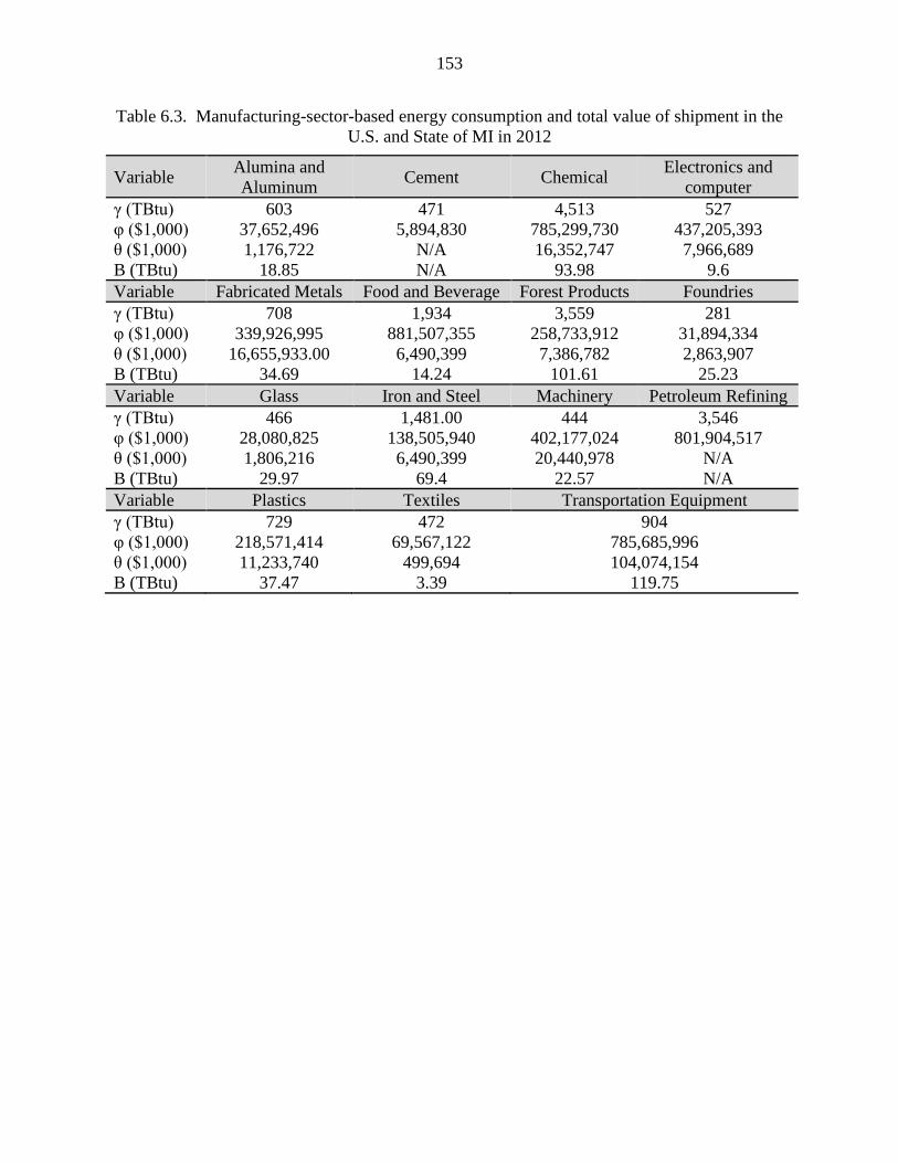
153
Table 6.3. Manufacturing-sector-based energy consumption and total value of shipment in the
U.S. and State of MI in 2012
Variable Alumina and
Aluminum Cement Chemical
Electronics and
computer
γ (TBtu) 603 471 4,513 527
φ ($1,000) 37,652,496 5,894,830 785,299,730 437,205,393
θ ($1,000) 1,176,722 N/A 16,352,747 7,966,689
B (TBtu) 18.85 N/A 93.98 9.6
Variable Fabricated Metals Food and Beverage Forest Products Foundries
γ (TBtu) 708 1,934 3,559 281
φ ($1,000) 339,926,995 881,507,355 258,733,912 31,894,334
θ ($1,000) 16,655,933.00 6,490,399 7,386,782 2,863,907
B (TBtu) 34.69 14.24 101.61 25.23
Variable Glass Iron and Steel Machinery Petroleum Refining
γ (TBtu) 466 1,481.00 444 3,546
φ ($1,000) 28,080,825 138,505,940 402,177,024 801,904,517
θ ($1,000) 1,806,216 6,490,399 20,440,978 N/A
B (TBtu) 29.97 69.4 22.57 N/A
Variable Plastics Textiles Transportation Equipment
γ (TBtu) 729 472 904
φ ($1,000) 218,571,414 69,567,122 785,685,996
θ ($1,000) 11,233,740 499,694 104,074,154
B (TBtu) 37.47 3.39 119.75
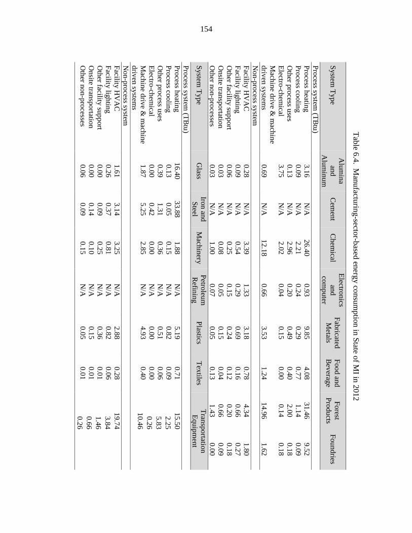
154
Tab
le 6.4
. Man
ufactu
ring-secto
r-based
energ
y co
nsu
mptio
n in
State o
f MI in
2012
System
Type
Alu
min
a
and
Alu
min
um
Cem
ent
Chem
ical
Electro
nics
and
com
puter
Fab
ricated
Metals
Food an
d
Bev
erage
Forest
Pro
ducts
Foundries
Pro
cess system
(TB
tu)
Pro
cess heatin
g
3.1
6
N/A
26.4
0
0.9
3
9.8
5
4.0
8
31.4
6
9.5
2
Pro
cess coolin
g
0.0
9
N/A
2.2
1
0.2
4
0.2
9
0.7
7
1.1
4
0.0
9
Oth
er pro
cess uses
0.1
3
N/A
2.9
6
0.2
0
0.4
9
0.4
0
2.0
0
0.1
8
Electro
-chem
ical 3.7
5
N/A
2.0
2
0.0
4
0.1
5
0.0
0
0.1
4
0.1
8
Mach
ine d
rive &
mach
ine
driv
en sy
stems
0.6
9
N/A
12.1
8
0.6
6
3.5
3
1.2
4
14.9
6
1.6
2
Non-p
rocess sy
stem
Facility
HV
AC
0.2
8
N/A
3.3
9
1.3
3
3.1
8
0.7
8
4.3
4
1.8
0
Facility
lightin
g
0.0
9
N/A
0.5
4
0.2
9
0.6
9
0.1
6
0.6
6
0.2
7
Oth
er facility su
pport
0.0
6
N/A
0.2
5
0.1
5
0.2
4
0.1
2
0.2
0
0.1
8
Onsite tran
sportatio
n
0.0
3
N/A
0.0
8
0.0
5
0.1
5
0.0
4
0.6
6
0.0
9
Oth
er non-p
rocesses
0.0
3
N/A
1.0
0
0.0
7
0.0
5
0.1
3
1.4
3
0.0
0
System
Type
Glass
Iron an
d
Steel
Mach
inery
P
etroleu
m
Refin
ing
P
lastics T
extiles
Tran
sportatio
n
Equip
men
t
Pro
cess system
(TB
tu)
Pro
cess heatin
g
16.4
0
33.8
8
1.8
8
N/A
5.1
9
0.7
1
15.5
0
2.2
5
5.8
3
0.2
6
10.4
6
Pro
cess coolin
g
0.1
3
0.0
5
0.1
5
N/A
0.8
2
0.0
9
Oth
er pro
cess uses
0.3
9
1.3
1
0.3
6
N/A
0.5
1
0.0
6
Electro
-chem
ical 0.0
0
0.4
2
0.0
0
N/A
0.0
0
0.0
0
Mach
ine d
rive &
mach
ine
driv
en sy
stems
1.8
7
5.2
5
2.8
5
N/A
4.9
3
0.4
0
Non-p
rocess sy
stem
Facility
HV
AC
1.6
1
3.1
4
3.2
5
N/A
2.8
8
0.2
8
19.7
4
3.8
4
1.4
6
0.6
6
0.2
6
Facility
lightin
g
0.2
6
0.3
7
0.8
1
N/A
0.8
2
0.0
6
Oth
er facility su
pport
0.0
0
0.0
9
0.2
5
N/A
0.3
6
0.0
1
Onsite tran
sportatio
n
0.0
0
0.1
4
0.1
0
N/A
0.1
5
0.0
1
Oth
er non-p
rocesses
0.0
6
0.0
9
0.1
5
N/A
0.0
5
0.0
1

155
Energy loss estimation. Energy loss calculation is completed using Table 6.2 data and Eqs.
6.13-6.17. According to ACEEE (2012), MI’s ranking on energy efficiency is 12 in the nation.
This ranking number is the value of Rs in Eq. 6.13. Table 6.5 shows the manufacturing-sector-
based energy loss percentage in MI in 2012, while Table 6.6 lists the detailed process and non-
process energy loss in different manufacturing sectors in MI, which is calculated using the data in
Tables 6.2, 6.4, and 6.5 and Eqs. 6.14-6.15. Comparison of the corresponding values in Table 6.2
(for the U.S.) and Table 6.5 (for MI) shows MI’s energy loss in each manufacturing sector is
clearly less than the national average. The total amount of direct energy loss in MI’s
manufacturing sector ( s,totEL ) is 132.06 TBtu, which includes the process energy loss of 108.42
TBtu (i.e., 17.7% of the total energy consumption or 41.3% of the process energy consumption),
and the non-process energy loss of 23.64 TBtu (i.e., 3.9% of the total energy consumption or 35.3%
of the non-process energy consumption).
CO2 emission estimation. The energy footprint analysis is completed by the analysis of
energy-related CO2 emission of manufacturing sectors at the state level. Using Eqs. 6.7 and 6.18-
6.20, the total energy-related CO2 emission for each sector in MI is estimated, and the same
approach is used for estimation in other states. The estimation results are plotted in Fig. 6.3. The
summarized estimation shows that in 2012, the total manufacturing combustion (energy-related
CO2) emission of all 51 states was 1,134 MMT CO2e, which shows 10% difference as compared
to the value from the national reported, which does not contain any state-based manufacturing
sector specific information on CO2 emission (U.S. DOE, 2012). Thus, the estimation by the
introduced methodology is quite satisfactory.

156
Tab
le 6.5
. Man
ufactu
ring-secto
r-based
energ
y lo
ss percen
tage in
MI in
20
12
System
Type
Alu
min
a
and
Alu
min
um
Cem
ent
Chem
ical
Electro
nics
and
com
puter
Fab
ricated
Metals
Food an
d
Bev
erage
Forest
Pro
ducts
Foundries
Pro
cess system
Pro
cess heatin
g
43.4
3
34.2
9
18.9
2
32.0
4
32.5
2
57.7
5
55.0
2
43.8
1
Pro
cess coolin
g
28.6
7
0.0
0
30.0
2
33.0
8
28.6
7
30.3
0
30.1
0
0.0
0
Oth
er pro
cess uses
0.0
0
0.0
0
8.4
8
7.8
2
8.6
0
9.3
8
8.6
0
0.0
0
Electro
-chem
ical 51.6
0
0.0
0
51.4
2
43.0
0
57.3
3
0.0
0
51.6
0
43.0
0
Mach
ine d
rive &
mach
ine
driv
en sy
stems
39.0
9
66.1
5
62.3
3
52.5
6
53.7
5
56.3
1
50.0
6
43.0
0
Non-p
rocess sy
stem
Facility
HV
AC
28.6
7
21.5
0
30.0
7
29.4
5
30.4
3
30.0
2
29.9
9
30.1
0
Facility
lightin
g
86.0
0
86.0
0
76.0
8
75.2
5
73.7
1
78.1
8
78.5
2
86.0
0
Oth
er facility su
pport
0.0
0
0.0
0
7.1
7
10.7
5
17.2
0
10.7
5
12.2
9
0.0
0
Onsite tran
sportatio
n
86.0
0
43.0
0
43.0
0
57.3
3
57.3
3
51.6
0
52.3
5
86.0
0
Oth
er non-p
rocesses
0.0
0
0.0
0
8.9
6
0.0
0
0.0
0
10.1
2
8.6
0
0.0
0
System
Type
Glass
Iron an
d
Steel
Mach
inery
P
etroleu
m
Refin
ing
P
lastics T
extiles
Tran
sportatio
n
Equip
men
t
Pro
cess system
Pro
cess heatin
g
48.2
3
43.8
9
32.5
4
15.4
7
18.7
3
58.2
0
32.3
4
30.3
5
7.8
2
43.0
0
53.3
4
Pro
cess coolin
g
43.0
0
86.0
0
28.6
7
32.2
5
32.2
5
28.6
7
Oth
er pro
cess uses
14.3
3
9.2
1
12.2
9
8.8
4
8.6
0
9.5
6
Electro
-chem
ical 0.0
0
57.3
3
0.0
0
0.0
0
0.0
0
0.0
0
Mach
ine d
rive &
mach
ine
driv
en sy
stems
53.3
8
41.4
6
53.7
5
57.1
4
53.7
5
54.7
3
Non-p
rocess sy
stem
Facility
HV
AC
30.9
30.8
1
30.9
1
29.3
7
30.7
1
30.8
7
30.0
1
77.1
0
7.8
2
51.6
0
0.0
0
Facility
lightin
g
86.0
0
75.2
5
75.2
5
86.0
0
75.2
5
76.4
4
Oth
er facility su
pport
0.0
0
0.0
0
17.2
0
0.0
0
12.2
9
0.0
0
Onsite tran
sportatio
n
0.0
0
57.3
3
43.0
0
86.0
0
57.3
3
86.0
0
Oth
er non-p
rocesses
0.0
0
0.0
0
0.0
0
7.1
7
0.0
0
0.0
0

157
T
able 6
.6. M
anufactu
ring-secto
r-based
energ
y lo
ss in M
I in 2
012
System
Type
Alu
min
a
and
Alu
min
um
Cem
ent
Chem
ical
Electro
nics
and
com
puter
Fab
ricated
Metals
Food an
d
Bev
erage
Forest
Pro
ducts
Foundries
Pro
cess system
(TB
tu)
Pro
cess heatin
g
1.3
7
N/A
5.0
0
0.3
0
3.2
0
2.3
6
17.3
1
4.1
7
Pro
cess coolin
g
0.0
3
N/A
0.6
6
0.0
8
0.0
8
0.2
3
0.3
4
0.0
0
Oth
er pro
cess uses
0.0
0
N/A
0.2
5
0.0
2
0.0
4
0.0
4
0.1
7
0.0
0
Electro
-chem
ical 1.9
4
N/A
1.0
4
0.0
2
0.0
8
0.0
0
0.0
7
0.0
8
Mach
ine d
rive &
mach
ine
driv
en sy
stems
0.2
7
N/A
7.5
9
0.3
4
1.9
0
0.7
0
7.4
9
0.7
0
Non-p
rocess sy
stem (T
Btu
)
Facility
HV
AC
0.0
8
N/A
1.0
2
0.3
9
0.9
7
0.2
3
1.3
0
0.5
4
Facility
lightin
g
0.0
8
N/A
0.4
1
0.2
2
0.5
1
0.1
3
0.5
2
0.2
3
Oth
er facility su
pport
0.0
0
N/A
0.0
2
0.0
2
0.0
4
0.0
1
0.0
2
0.0
0
Onsite tran
sportatio
n
0.0
3
N/A
0.0
4
0.0
3
0.0
8
0.0
2
0.3
4
0.0
8
Oth
er non-p
rocesses
0.0
0
N/A
0.0
9
0.0
0
0.0
0
0.0
1
0.1
2
0.0
0
System
Type
Glass
Iron an
d
Steel
Mach
inery
P
etroleu
m
Refin
ing
P
lastics T
extiles
Tran
sportatio
n
Equip
men
t
Pro
cess system
(TB
tu)
Pro
cess heatin
g
7.9
1
14.8
7
0.6
1
N/A
0.9
7
0.4
1
5.0
1
0.6
8
0.4
6
0.1
1
5.5
8
Pro
cess coolin
g
0.0
6
0.0
4
0.0
4
N/A
0.2
7
0.0
2
Oth
er pro
cess uses
0.0
6
0.1
2
0.0
4
N/A
0.0
4
0.0
1
Electro
-chem
ical 0.0
0
0.2
4
0.0
0
N/A
0.0
0
0.0
0
Mach
ine d
rive &
mach
ine
driv
en sy
stems
1.0
0
2.1
8
1.5
3
N/A
2.6
5
0.2
2
Non-p
rocess sy
stem (T
Btu
)
Facility
HV
AC
0.5
0
0.9
7
1.0
1
N/A
0.8
8
0.0
9
5.9
2
2.9
6
0.1
1
0.3
4
0.0
0
Facility
lightin
g
0.2
2
0.2
8
0.6
1
N/A
0.6
2
0.0
5
Oth
er facility su
pport
0.0
0
0.0
0
0.0
4
N/A
0.0
4
0.0
0
Onsite tran
sportatio
n
0.0
0
0.0
8
0.0
4
N/A
0.0
9
0.0
1
Oth
er non-p
rocesses
0.0
0
0.0
0
0.0
0
N/A
0.0
0
0.0
0

158
Ma
nu
factu
ring
Ca
rbo
n
Dio
xid
e Em
ission
<=
15
MM
T
15-3
0 M
MT
30
-60
MM
T
60
-95
MM
T
95
-20
0 M
MT
Fig
ure 6
.3. M
anu
facturin
g carb
on d
iox
ide em
ission m
ap.

159
County-level energy analysis. Sector-based energy consumption at the county level can
be estimated using Eqs. 6.21-6.22, and the total energy consumption of all manufacturing sectors
in a county using Eq. 6.23 (see Fig. 6.4). In this case study, as we have selected the state of
Michigan (MI) at the state level estimation, the counties of MI are used in our calculation. The
state has 83 counties. The sector-based direct energy loss of each county is calculated using Eqs.
6.24-6.26. In Michigan, the three most energy-intensive counties are Wayne County, Oakland
County, and Macomb County, and the numbers of manufacturing establishments in these counties
are 1,483, 1,669, and 1,593, respectively (USCS, Table EC1231SA1). Table 6.7 shows the total
values of SSR of the eight main manufacturing sectors in these counties (USCS, Table
EC1231A1), while Table 6.8 gives the estimated energy consumption and direct energy loss of
each of the eight manufacturing sectors in these counties. The CO2 emission estimations for the
state as well as the eight manufacturing sectors of the three countries are shown in Table 6.9. The
total manufacturing energy consumption, energy loss, and energy-related CO2 emission of the
three counties are shown in Fig. 6.5. Note that the same approach was used to generate estimations
of energy consumption and energy loss in seven other manufacturing sectors; the estimation result
is omitted here.

160
Table 6.7. Total value of shipment for manufacturing sectors in three energy intensive counties
in MI
Region
Chemical Electronics and
Computer Fabricated Metals
Food and
Beverage
Total Value of
shipment- ω
($1000)
Total Value of
shipment- ω
($1000)
Total Value of
shipment- ω
($1000)
Total Value of
shipment- ω
($1000)
Wayne 1,907,458 1,099,542 2,077,699 859,989
Oakland 1,219,885 1,045,018 2,138,317 N/A
Macomb 760,934 277,267 2,398,485 92,176
Region
Forest Products Machinery Plastics Transportation
Equipment
Total Value of
shipment- ω
($1000)
Total Value of
shipment- ω
($1000)
Total Value of
shipment- ω
($1000)
Total Value of
shipment- ω
($1000)
Wayne 441,938 3,282,221 861,696 34,981,849
Oakland 89,144 3,992,381 846,207 6,693,498
Macomb 56,699 2,630,031 996,818 18,696,841
Figure 6.4. Manufacturing energy consumption in counties of Michigan.
Manufacturing Energy Consumption
0-1 TBtu
1-6 TBtu
6-15 TBtu
45-100 TBtu
>=100 TBtu

161
Table 6.8. Manufacturing-sector-based energy consumption and direct loss in three energy
intensive counties in MI
Region Chemical Electronics and Computer
ECC (TBtu) ELC (TBtu) ECC (TBtu) ELC (TBtu)
Wayne 10.96 1.88 1.33 0.19
Oakland 7.01 1.2 1.26 0.19
Macomb 4.37 0.75 0.33 0.05
Region Fabricated Metals Food and Beverage
ECC (TBtu) ELC (TBtu) ECC (TBtu) ELC (TBtu)
Wayne 4.33 0.86 1.89 0.49
Oakland 4.45 0.89 N/A N/A
Macomb 5 1 0.2 0.05
Region Forest Products Machinery
ECC (TBtu) ELC (TBtu) ECC (TBtu) ELC (TBtu)
Wayne 6.08 1.66 3.62 0.63
Oakland 1.23 0.33 4.41 0.77
Macomb 0.78 0.21 2.9 0.51
Region Plastics Transportation Equipment
ECC (TBtu) ELC (TBtu) ECC (TBtu) ELC (TBtu)
Wayne 2.87 0.43 40.25 7.12
Oakland 2.82 0.42 7.7 1.36
Macomb 3.32 0.49 21.51 3.81
Table 6.9. Carbon dioxide emission of MI and three counties with respect to manufacturing
sectors
Sector/Region Michigan
(MMT)
Wayne
(MMT)
Oakland
(MMT)
Macomb
(MMT)
Chemical 5.73 0.67 0.43 0.27
Electronics and
Computer 0.56 0.08 0.07 0.02
Fabricated Metals 2.01 0.25 0.26 0.29
Food and Beverage 0.86 0.11 0 0.01
Forest Products 4 0.24 0.05 0.03
Machinery 1.32 0.21 0.26 0.17
Plastics 2.26 0.17 0.17 0.2
Transportation
Equipment 7.02 2.36 0.45 1.26
Total 32.67 7.74 2.52 3.69

162
Figure 6.5. Energy consumption, energy loss, and carbon dioxide emission of three energy
intensive counties in MI.
6.3 Summary
Energy efficiency in the manufacturing industry is continuously one of the most critical
factor in energy sustainability and thus the nation’s economic, environmental, and social
sustainability. A variety of energy and related CO2 emission information and data are openly
accessible, which were generated with possibly different purposes, under different assumptions,
focusing on different time periods, and by different organizations. Integrated use of the accessible
information could generate very valuable information on energy and CO2 footprint in the
geographical regions of interest.
In this chapter, we have introduced a simple, general energy efficiency and CO2 emission
analysis method for energy use performance estimation in manufacturing industries in different
Oakland County
Wayne
County
Detroit
Note:
ECc =Manufacturing Energy Consumption (TBtu)
ELc =Manufacturing Energy Loss-Direct use(TBtu)
CEc =Manufacturing Energy-Related CO2 Emission (MMT)
ESTAB= No. of Manufacturing Establishments (year 2012)
State of
Michigan

163
geographical regions. The case study has demonstrated methodological efficacy, as we are able
to identify the performance of different manufacturing sectors in terms of the amount of energy
used and lost in various energy-consuming systems, and CO2 emission of individual state and thus
county in the U.S. The study has been also applied to the state of Michigan and its counties, which
has provided a better insight for the possible improvement directions.

164
CHAPTER 7 CONCLUSIONS AND FUTURE WORK
In this chapter, the dissertation objectives and the contributions are summarized in the first
section. Recommendations for the possible extension of this research and future work is discussed
in the second part.
7.1 Conclusions
Improvement of energy efficiency in process systems has been always a key concern in the
chemical process industry. However, the recovery of mechanical energy, as compared to thermal
energy recovery, has not received sufficient attention. This renders a research need on work
integration through designing WEN for chemical plants.
This research has focused on the recovery of mechanical energy using work exchangers
that were introduced by Cheng et al. (1967). A general review of the current research progress is
provided, together with a basic thermodynamic analysis on work exchange, the challenges and
opportunities. This facilitates the introduction of a mathematical modeling and analysis method
which aims at predicting the maximum amount of mechanical energy that can be feasibly
recovered using work exchangers.
The thermodynamic modeling and analysis method is a general tool to predict the
maximum amount of mechanical energy recoverable by a WEN prior to network synthesis for any
design problem. The methodology referred to as prediction stage can be easily modified based on
the operation condition, phase, and also when combined with a heat or mass exchange network.
The modification does not change the structure of the methodology and only the shaft work
formulation will differ.
Using the mathematical framework provided in the prediction stage, the work exchange
network synthesis can be completed by the set of matrices and vectors which identify the
placement of work exchangers, utility compressors and expanders if needed. Similar to the

165
prediction stage, the formulation is general and can be extended to different operating conditions,
assumptions, and energy calculations. Note that the temperature will change through the
pressurization and depressurization processes when dealing with gas phase streams. Through the
process of compression, temperature increases, which means that heat will be added to the system,
and temperature decreases through the expansion, which means that heat will be consumed. In
addition, the energy required for compression decreases while the stream that goes through
pressurization has a lower temperature, and the energy provided through expansion increases while
the stream has a higher temperature. Therefore, due to the pressure and temperature correlation in
pressurization and depressurization, heat integration would play a key role in cases under non-
isothermal conditions. In fact, heat integration would be required for these cases not only for
thermal energy recovery but also for improving the amount of mechanical energy that can be
recovered. In Chapter 4, the integration of a heat exchanger network (HEN) into the work
exchanger network synthesis is discussed and it has been shown that the location of the HEN will
impact the amount of thermal and mechanical energy recovery. In the presented framework, the
final location of the HEN is assigned based on the lowest operating cost which reflects the design
with lower utility consumption. The methodological efficacy is illustrated by case studies, where
both mechanical and thermal energy efficiencies as well as an economic feasibility analysis are
provided.
In this study, a direct work exchanger has been considered as the mechanical energy
recovery device for the development of work exchange network synthesis. This unit was
introduced for reverse osmosis processes and has been used in the desalination industry due to its
distinctive performance. However, the device has not been considered for mechanical energy
recovery in other industries such as the chemical and petrochemical industries. Different

166
characteristics of the chemical processes require investigation into the operational flexibility of the
unit, and challenges related to the unit safety. In Chapters 2-4, we discussed the piston-type direct
work exchanger’s fundamentals, and introduced a thermodynamic analysis approach to design a
work exchange network synthesis using the direct work exchangers in chemical processes. While
the feasibility of using these units has been shown by significant improvements in mechanical
energy recovery of process systems, how these units can be implemented in real industrial
processes is still under investigation. Due to lack of computational and experimental studies on
piston-type direct work exchangers operated by gas phase streams, we have conducted research on
modeling of the unit using simulation software. The customized model has been generated by
Aspen Plus simulation software which helps us to add the work exchanger to the Aspen Plus unit
operations library and be able to simulate the synthesized work exchange network using direct
work exchangers, compressors, and expanders. This will ensure the design feasibility and
optimum operating conditions. The model formulation can be easily modified in the future as the
piston-type work exchanger develops. Computational Fluid Dynamics (CFD) modeling has been
studied for better understating of the operational behavior of the unit. We have been able to plot
the four operation stages of pressurization and depressurization in terms of piston motion, high-
pressure and low-pressure streams pressure profiles, and valve positions. In addition, the
performance of a unit under various operating conditions such as pressure and temperature is
investigated. This is a significant accomplishment towards modification of the piston-type work
exchangers dealing with gas phase streams.
Energy efficiency in manufacturing systems becomes increasingly critical in energy
sustainability due to a trend toward the depletion of non-renewable resources and the challenges
owing to carbon dioxide (CO2) emission. For better evaluation of energy consumption in

167
manufacturing industries, various energy consumption-related databases have been created by a
number of research studies and government agencies. However, a general methodology to study
the energy efficiency of manufacturing sectors in various geographical scales is not available. In
Chapter 6, we proposed a general data-driven methodology for energy efficiency and CO2
emission analysis of manufacturing sectors in different geographical scopes. The analysis method
can be used as a baseline to identify the performance of different manufacturing sectors in terms
of the amount of energy that will be used or lost for various systems, and the combustion emission
of each state across the U.S. and its counties. The study has been also applied to the state of
Michigan as a case study and its counties to have a better insight on improvement directions and
to support the future of the energy advancement in industries. Future analysis will look to further
combine the methodology with decision making modules for energy efficiency improvement in
different geographical areas.
7.2 Future Work
The dissertation establishes a solid knowledge foundation for the research related to
mechanical energy recovery through a work exchange network synthesis approach. This section
discusses the possible extension of this research for future development.
Optimization-based heat integrated work exchange network synthesis. The superstructure-
based framework has been considered in heat exchanger network synthesis by the chemical
industries to find the local optimum design and for more complicated problems. A superstructure-
based simultaneous heat and work exchange network has been also studied using SSTC
compressors and turbines counted as the indirect work exchangers. This framework can be also
extended for designs in which direct work exchangers are implemented. The direct work
exchangers show a unique performance for mechanical energy recovery, and their feasibility for

168
work exchange network design has been demonstrated by the thermodynamic modeling approach.
Even though the energy targeting methodology and sequential flowsheet development generate a
WEN with the maximum energy recovery, the optimality of the design is not guaranteed. Thus,
development of superstructure methods to solve the heat and work exchange network synthesis
problems simultaneously and to find the optimum design is suggested. The objective function can
be taken as a minimization of the total annualized cost. In the following, the initial mathematical
formulation of a MINLP model regarding WEN synthesis is shown. However, comprehensive
study is still required to complete the mathematical formulation.
Decision variables can be stated as:
Pi,k, Pj,k = pressure of each HP and LP stream after each match
Wijk= workload of each work exchanger between HP and LP streams at stage k
WHPu,j= workload of HP external utility
WLPu, i = workload of LP external utility
1 if there is a work exchange r between stream i and j in stage k
0 if there is not a work exchanger between stream i and j in stage kijkz
,
1 if there is a HP utility for stream j
0 if there is not a HP utility for stream jHu jz
,
1 if there isa LP utility for stream i
0 if there is not a LP utility for stream iLu iz
The objective function can be written as:
Minimize

169
j,HPu
J
ji,LPu
I
i
HPu,j
J
j
HPu,jLPu,i
I
i
LPu,i
I
i
J
j
K
k
ijijj,Hu
J
j
HPu,j
i,Lu
I
i
J
j
K
k
I
i
LPu,iijkijTAC
WCHuWCLu
SCSC
SCzCF
zCFzCFC
11
11
1 1 11
1 1 1 1
(7.1)
Subject to:
)W(fS ijij 1 (7.2)
jkikjiij P,P,V,VfW 2 (7.3)
)W(fS i,LPuLPu,i 3 (7.4)
)P,P,P,V(fW t
i
s
iikii,LPu 4 (7.5)
)W(fS j,HPuHPu,j 5 (7.6)
)P,P,P,V(fW t
j
s
jjkjj,HPu 6 (7.7)
where
I: number of HP process streams
J: number of LP process streams
K: index for stage, and pressure location
LPu: low-pressure utility
HPu: high-pressure utility
Ps, Pt: source and target pressure
∆Pmin: minimum approach pressure difference
Vi, Vj: volumetric flowrates
CLu: per unit cost of LP utility
Chu: per unit cost of HP utility

170
CFij, CFi, LPu, CFj, HPu: fixed charges for exchangers
Cij, Ci, LPu, Cj, HPu: cost coefficient
Sij, Si, LPu, Sj, HPu: size factors of exchangers
The feasibility constraints, work balance at each stage, should be added later to complete
the mathematical formulation to solve the problem using appropriate optimization software. It is
suggested that the optimization be completed under isothermal conditions first to investigate the
work exchanger formulation feasibility, and then the non-isothermal conditions should be
considered for development of the heat integrated WEN synthesis superstructure. In addition,
phase behavior correlation of each high-pressure and low-pressure stream should be considered.
Development of appropriate user interface for work exchange network synthesis. In
Chapters 3 and 4, a mathematical formulation was presented which will predict the maximum
amount of mechanical energy that can be recovered and will provide the information regarding the
placement of work exchangers, external compressors, and external expanders through a set of
matrices and vectors. The formulation for the prediction stage has been developed in MATLAB
which will help users to easily calculate the amount of energy that can be recovered for a case
study of any size. However, it is recommended to develop a graphical user interface for the coded
methodology using the appropriate compiler. This will help users, especially industry, to
investigate work exchange network synthesis in processes in which mechanical energy is being
wasted and quickly define the feasibility and profitability of the technology.
CFD modeling verification by experiment. In Chapter 5, a preliminary investigation into
the operational behavior of piston-type work exchangers operated by gas phase streams was
presented. However, there are still different unit configurations that should be studied. The main
areas that the modeling should be extended can be summarized as: possible phase change through

171
the pressurization and depressurization of working fluids, dealing with different fluid domains at
each side of the piston, and non-reversible behavior of the compression and expansion due to
friction loss between the piston ring and the cylinder wall which will impact the shaft work
formulation. Working alongside IC engine experts will help to integrate the modeling for possible
manufacturing of the unit at the laboratory and pilot scale. This will help to address challenges
related to energy recovery of the device from the unit-based to network-based scale and will be a
beginning for commercializing the piston-type work exchangers operated by gas phase streams in
the chemical and petrochemical industry.
Minimum pressure difference optimization. After conducting the CFD modeling, we found
that how the pressure difference between two sides of the piston will impact the piston speed of
movement and the operational cycle. Previously, Cheng et al. (1967) analyzed the flow work
exchanger performance for reverse osmosis and concluded that the minimum pressure difference
for the piston motion should between 35 kPa to 70 kPa. This range could be significantly different
while dealing with different processes, working fluids with various compression ratios, and also
with the size and the materials used to manufacture the unit component parts. Thus, the minimum
pressure difference should be studied and optimized later using the results from the modeling and
pilot study validation.

172
APPENDICES
Appendix A
Appendix A contains the step-by-step derivation of matrices Γ and P using the flowchart
shown in Fig. 3.1 and Eqs. 3.3-3.7 for a case study from the Huang and Fan (1996) work.
Table A-1. Streams data for a case study from Huang and Fan (1996)
Stream No. Ps (MPa) Pt (MPa) V (m3/s)
H1 5.72 2.21 0.099
H2 3.10 0.26 0.076
L1 1.72 3.10 0.083
L2 0.10 2.21 0.050
L3 0.51 5.72 0.073
For this case study with two high-pressure streams and three low-pressure streams:
2HN ; 3LN
Construct matrix Γ
In this case study Γ is a 32 matrix and minP is assumed to be 0.07 MPa. Each element
of Γ is constructed using the flowchart shown in Figure 2.
322212
312111
L,HL,HL,H
L,HL,HL,H
ΓΓΓ
ΓΓΓΓ (A-1)
For b
L,H
a
L,HL,H1111
11Γ,ΓΓ :
Calculation ofa
L,H 11Γ
07011
. t
H
s
L PP (A-2)
070212721 ... => Yes (A-3)
and
t
L
t
H
s
L PPP111
070 . (A-4)

173
103070212721 .... => Yes (A-5)
Then,
MPa282
070111
.
.,
t
H
a
LH PΓ (A-6)
Calculation of b
L,H 11Γ
07011
. t
L
s
H PP (A-7)
where
070103725 ... => NO (A-8)
Then,
MPa103
1
.
t
L
b
L,H PΓ11
(A-9)
Then,
103282 .,.11 L,HΓ (A-10)
For b
LH
a
LHLH ΓΓΓ1212
12 ,,, , :
Calculation of a
LHΓ 12 ,
07021
. t
H
s
L PP (A-11)
070260721 ... => No (A-12)
Then,
MPa721
112
.
,
s
L
a
LH PΓ (A-13)
Calculation of b
LHΓ 12 ,
07012
. t
L
s
H PP (A-14)

174
where
070103103 ... => Yes (A-15)
and
t
L
s
H
s
L PPP121
070 . (A-16)
103070103721 .... => Yes (A-17)
Then,
MPa033
070212
.
.,
s
H
b
LH PΓ (A-18)
Then,
03372112
.,., LHΓ (A-19)
For b
LH
a
LHLH ΓΓΓ2121
21 ,,, ,
Calculation of a
LHΓ 21 ,
07012
. t
H
s
L PP (A-20)
070212100 ... => Yes (A-21)
and
t
L
t
H
s
L PPP212
070 . (A-22)
212070212100 .... => No (A-23)
Then,
021a
LHΓ , (A-24)
Calculation of b
LHΓ 21 ,
07021
. t
L
s
H PP (A-25)

175
where
070212725 ... => No (A-26)
Then,
021b
LHΓ , (A-27)
and
0021
,, LHΓ (A-28)
Going through the same procedure, matrix Γ will be constructed.
033510212330033721
65528200103282
.,..,..,.
.,.,.,.Γ (A-29)
Construct matrix P
322212
312111
LHLHLH
LHLHLH
PPP
PPP
,,,
,,,P , (A-30)
and 0 but 1 k k and 20 ki .
For b
LH
a
LHLH PPP1111
11 ,,, , :
where 111 kij ;; => 2110 OK
otherwise
if 21
11
1
;
;
,
12111111
11
L,HL,HL,HL,H
HHL,H
LH
RΓΓ
VVΓ
P ; (A-31)
and
smVsmV HH /.;/.33 076300990
21 (A-32)
Then,

176
103282 .,.
1111 L,H
1
L,H ΓP (A-33)
where 111 kij ;; => 2110 will not be met.
Then,
existnotdoes1
11
LHP , (A-34)
and
103282
11
111111
.,.
, ,,,
LHLHLH PPP (A-35)
For b
LH
a
LHLH PPP1212
12 ,,, , :
where 121 kij ;; => 2120 will not be met.
Then,
existnotdoes1
12 LHP , (A-36)
where 121 kij ;; => 2120 OK
otherwise
if
121212
1212
12
1
;
;
,,
,
,
11 L,HL,HLHLH
HHLH
LH
RΓΓ
VVΓ
P ; (A-37)
and
smVsmV HH /.;/.33 0990007630
12 (A-38)
Then,
11 L,HL,HLHLHLH RΓΓP12
121212
1
,,, (A-39)
where

177
033282
103033282721
1112111212
.,.
..,..
, ,,,,
b
LH
b
LH
a
LH
a
LHL,HL,H ΓΓΓΓR11
(A-40)
Then,
282721
0332820337210337211
12
.,.
.,..,..,.,
LHP (A-41)
and
282721
11
121212
.,.
, ,,,
LHLHLH PPP (A-42)
Going through the same procedure, matrix P will be constructed.
282510212330282721
65528200103282
.,..,..,.
.,.,.,.P (A-43)
Appendix B
Appendix B contains the MATLAB code written for calculation of the prediction
methodology discussed in Chapter 3. As a sample, the code for calculating maximum energy
recovery using the prediction methodology is shown for case 2 from Chapter 4 (Table 4.5).
function [Result,WR,WR2,Whpu,Wlpu,Pa,Pb,dM,WM,Wm,dQ,WQ,WG]=
casestudy41(I,J,WHTOTAL,WLTOTAL,Phs,Pht,Pls,Plt,dpmin,rs,etta,ml,mh,Ths,Tht,T
ls,Tlt) I=3; J=2; %WHTOTAL=2771.1; %WLTOTAL=3406.1; Phs=[900;850;700]; Ths=[350;350;400]; Pht=[100;150;200]; Tht=[350;350;400]; Pls=[100;100]; Tls=[390;420]; Plt=[700;900]; Tlt=[390;420]; dpmin=70; rs=1.4; etta=1;

178
ml=[25.78;36.81]; mh=[36.81;14.73;21.48]; %Rh=[0.347662;0.337287;0.248735]; %Rl=[0.641965;0.630812]; %Cph=[1.432;0.982;1.046]; %Cpl=[1.432;1.432]; dQ=zeros((I*(I-1)/2),J); WG = zeros(1, I); Wexp= zeros(1, I); Wcomp= zeros(1, I); N=zeros(1,(I*(I-1)/2)); N1=zeros(1,(I*(I-1)/2)); N2=zeros(1,(I*(I-1)/2)); %M matrix represent the italic p matrix %Q matrix represent the italic O matrix %G matrix represent the italic wo matrix %Wleft matrix represent the italic WL matrix for j=1:J for i=1:I if Phs(i)>=Plt(j)+dpmin Pa(i,j)=Plt(j) elseif Pls(j)<Phs(i)-dpmin & Phs(i)-dpmin<Plt(j) Pa(i,j)=Phs(i)-dpmin else Pa(i,j)=0 end if Pls(j)>=Pht(i)+dpmin Pb(i,j)=Pls(j) elseif Pls(j)<Pht(i)+dpmin & Pht(i)+dpmin<Plt(j) Pb(i,j)=Pht(i)+dpmin else Pb(i,j)=0 end if Pa(i,j)==0 Pb(i,j)=0 elseif Pb(i,j)==0 Pa(i,j)=0 else end %alpha(j)=Rl(j)/Cpl(j); %Betta(i)=Rh(i)/Cph(i); dM(i,j)=[(((Pa(i,j)/Pb(i,j))^((rs-1)/rs))-1)*(1+(Pb(i,j)/Pls(j))^((rs-1)/rs)-
1)] Vl(j)=ml(j)*Tls(j)
Vh(i)=mh(i)*Ths(i) end end WM=dM*diag(Vl)*etta; d=ones(J,1) Wm=WM*d for i=1:I Wh(i)=Vh(i)*(1-(Pht(i)/Phs(i))^((rs-1)/rs)) Wt(i)=Wh(i)-Wm(i) end for j=1:J n=1

179
for i=1:I for k=i+1:I if (Pb(i,j)==0 & Pa(i,j)==0) N(1,n)=0 N1(1,n)=min(Vh(i),Vh(k)) elseif (Pb(k,j)==0 & Pa(k,j)==0) N(1,n)=0 N1(1,n)=min(Vh(i),Vh(k)) else
N(1,n)=((max(intersect(Pb(i,j):0.01:Pa(i,j),Pb((k),j):0.01:Pa((k),j)))/min(in
tersect(Pb(i,j):0.01:Pa(i,j),Pb((k),j):0.01:Pa((k),j))))^((rs-1)/rs))-1 N1(1,n)=min(Vh(i),Vh(k))
N2(1,n)=ml(j)*Tls(j)*(etta)*(1+(min(intersect(Pb(i,j):0.01:Pa(i,j),Pb((k),j):
0.01:Pa((k),j)))/Pls(j))^((rs-1)/rs)-1) end n=n+1;
end end for s=1:n-1 dQ(s,j)=N(1,s) E(s,j)=N1(1,s) VV(s,j)=N2(1,s) end end WQ=dQ.*VV for j=1:J for s=1:(I*(I-1))/2 if s+1>(I*(I-1))/2 break elseif WQ(s,j)==WQ(s+1,j) WQ(s+1,j)=0 else end end end for s=1:(I*(I-1))/2 for j=1:J for i=1:I if E(s,j)==Vh(i) WG(i)= WG(i)+ WQ(s,j) else WG(i)=WG(i)+0 end
end end end for j=1:J for i=1:I WF(i)=Wt(i)+WG(i)
WL(j)=Vl(j)*((Plt(j)/Pls(j))^((rs-1)/rs)-1) d1=ones(1,I);

180
d2=ones(1,(I*(I-1)/2)); % Wq=d2*WQ; % Wmm=d1*WM; % Wleft(j)=Wq(j)-WL(j)-Wmm(j) if WF(i)>=0 Wexp(i)=WF(i) else Wexp(i)=0 end if WF(i)<=0 Wcomp(i)=WF(i); else Wcomp(i)=0 end end end d3=ones(I,1); d4=ones(J,1); d5=ones(1,I); Wlpu=Wexp*d3 wleft=WL*d4-(d5*Wm-WG*d3) Whpu=abs(Wcomp*d3)+abs(wleft) WR=WL*d4-Whpu WR2=Wh*d3-Wlpu WHTOTAL=Wh*d3 WLTOTAL=WL*d4 Result=[WHTOTAL;WLTOTAL;WR;WR2;Whpu;Wlpu] end
Appendix C
Appendix C includes the customized code listing-subroutine for the direct work exchanger
modeled in Aspen Plus. Note that only the parts that are highlighted in red have been modified
using the code provided by Aspen Plus for USER 2 unit operation (Aspen Tech, Getting Started
Customizing Unit Operation Models, 2013).
The code is listed and edited as follows.
C C User2 Unit Operation Model Subroutine for Excel Models C C This routine is used by default to communicate with User-Written C Excel Unit Operation models. The feed streams, and user-defined C real and integer parameters are automatically copied to Excel. C The workbook calculations are invoked and the Aspen Plus C simulation is updated with the product streams, and user-defined C real and integer parameters that were calculated by the Excel C Workbook. SUBROUTINE WE2 (NMATI, MSIN, NINFI, SINFI, NMATO, 2 SOUT, NINFO, SINFO, IDSMI, IDSII,

181
3 IDSMO, IDSIO, NTOT, NSUBS, IDXSUB, 4 ITYPE, NINT, INTV, NREAL, REALV, 5 IDS, NPO, NBOPST, NIWORK, IWORK, 6 NWORK, WORK, NSIZE, ESIZE, INTSIZ, 7 LD ) C IMPLICIT NONE C C DECLARE VARIABLES USED IN DIMENSIONING C INTEGER NMATI, NINFI, NMATO, NINFO, NTOT, + NSUBS, NINT, NPO, NIWORK,NWORK, + NSIZE C C DECLARE ARGUMENTS C INTEGER IDSMI(2,NMATI), IDSII(2,NINFI), IDSMO(2,NMATO), + IDSIO(2,NINFO), IDXSUB(NSUBS), ITYPE(NSUBS), + INTV(NINT), IDS(2,3), NBOPST(6,NPO), + IWORK(NIWORK), INTSIZ(NSIZE), NREAL, LD REAL*8 MSIN(NTOT,NMATI), SINFI(NINFI), SOUT(NTOT,NMATO), + SINFO(NINFO), WORK(NWORK), ESIZE(NSIZE), + REALV(NREAL) C C-------------------- Aspen Plus Common Definitions ------------------- C #include "dms_errout.cmn" #include "ppexec_user.cmn" #include "dms_ncomp.cmn" #include "dms_plex.cmn" REAL*8 B(1) EQUIVALENCE (B(1),IB(1)) C C-------- Declare Aspen Plus utility functions that will be used ------ C INTEGER DMS_IRRCHK, DMS_IFCMNC C C--------------------- Local Variable Declarations -------------------- C INTEGER OFFSET, NUM_COLS, NUM_ROWS, RETCODE, LID, + IBLANK(2), KREAL(3), KINT(3), KINPUT(2), KOUTPUT(2), + LDATA, I,J,K, LEN, KDIAG, IDX(10), + LIDSC, NCD, C_OFF, ERRNUMBER, NUM_LINES, + SOURCE(16), HOL_STRLEN, SOR_LENGTH, SSID(2), IPROG(2), + DESC_LENGTH,KOUTSOL(3), EXCEL_NAME_LEN, + EXCEL_NAME(64), KINPSOL(3), + DESCRIPTION(128) INTEGER LABELS(2,9), ROWNAMES(2,NCOMP_NCC+9) !Moved LABELS and ROWNAMES declarations. INTEGER REALROWS(2,NTOT+1) CHARACTER*8 RealLabels(2) !Realparam row ID’s. REAL*8 INSTREAM(NTOT*NMATI),OUTSTREAM(NTOT*NMATO) C C--------------------------- Data Section ----------------------------- C

182
DATA KINPUT /4HINPU, 4HT / DATA KOUTPUT /4HOUTP, 4HUT / DATA KREAL /4HREAL, 4HPARA, 4HMS / DATA KINT /4HINTP, 4HARAM, 4HS / DATA KINPSOL /4HINP_, 4H , 4H / DATA KOUTSOL /4HOUT_, 4H , 4H / DATA IPROG /4HUSRX, 4HLS / DATA IBLANK /4HIMIS, 4HS / DATA LABELS /4HTOTF, 4HLOW , 2 4HTEMP, 4H , 3 4HPRES, 4H , 4 4HENTH, 4HALPY, 5 4HVAP , 4HFRAC, 6 4HLIQ , 4HFRAC, 7 4HENTR, 4HOPY , 8 4HDENS, 4HITY , 9 4HMOLE, 4H WT / DATA RealLabels /'R' , + 'W' / ! Labels for Realparam table C---------------------------------------------------------------------- C- Establish Excel link and call StartIteration Workbook Hook Function C CALL USRUTL_GETEXCEL(EXCEL_NAME, EXCEL_NAME_LEN) CALL StartIteration(RETCODE, EXCEL_NAME,64, IDS(1,1), 8) IF(RETCODE .NE. 0) GOTO 1000 C--------------- Build Aspen_Input Data Table ------------------------- C C The Excel Aspen_Input Sheet serves as the Aspen Plus interface for C the material feeds having liquid and vapor components. C C The component flow rates and stream variables will be entered into C column 1 as the Excel row identifier. A separate column will be C entered for each material feed stream. The number of rows equals C the number of components plus the number of stream properties (9). C C Place the 8 character component name (2 integer words) for all C conventional components (NCOMP_NCC) into the first column of C the Excel table (ROWNAMES). The Aspen Plus function, C DMS_IFCMNC, returns the start of the component id storage C location. OFFSET = DMS_IFCMNC('IDSCC') DO J=1, NCOMP_NCC I = OFFSET + 2*(J-1) + 1 ROWNAMES(1,J) = IB(I) ROWNAMES(2,J) = IB(I+1) END DO C Copy the Aspen Plus stream vector property names into the table. C There are 9 standard stream properties in a material vector. C DO K=1, 9 J = K + NCOMP_NCC ROWNAMES(1,J) = LABELS(1,K) ROWNAMES(2,J) = LABELS(2,K)

183
END DO NUM_ROWS = NCOMP_NCC+9 C C Copy the material feed variables into the table. Data for C each material stream will be placed in separate columns. C NMATI equals the number of material feeds. NUM_COLS = NMATI DO J=1, NUM_COLS OFFSET = (J-1)*(NCOMP_NCC+9) DO I=1, NUM_ROWS INSTREAM(OFFSET+I) = MSIN(I,J) END DO END DO C--------------- Send Aspen_Input table to Excel ---------------------- LDATA = 8*NUM_ROWS*NUM_COLS CALL WriteTable(RETCODE , KINPUT, 8 , NUM_ROWS, + ROWNAMES, 8 , NUM_COLS, IDSMI , + 8 , 2 , INSTREAM, LDATA ) IF (RETCODE .NE. 0) GO TO 1000 C C------------ Send Aspen_IntParams table to Excel --------------------- C C The Aspen_IntParams Excel sheet serves as the interface for the C User2 model integer parameters. C LDATA = 8*NINT CALL WriteTable(RETCODE, KINT, 12 , NINT , + IBLANK , 0 , 1 , IBLANK, + 0 , 1 , INTV,LDATA ) IF (RETCODE .NE. 0) GO TO 1000 C C-------------- Send Aspen_RealParams table to Excel ------------------- C C The Aspen_RealParams Excel sheet serves as the interface for the C User2 model real parameters. C LDATA = 8*NREAL CALL WriteTable(RETCODE, KREAL, 12 , NREAL , + IBLANK , 0 , 1 , IBLANK, + 0 , 2 , REALV,LDATA ) IF (RETCODE .NE. 0) GO TO 1000 C C-------- Initialize the Aspen_Output Excel table --------------------- C C The Aspen_Output Excel sheet serves as the interface for the C product streams having liquid and vapor components. This C initialization step is optional. NUM_ROWS=NCOMP_NCC+9 DO J=1, NMATO OFFSET = (J-1)*(NCOMP_NCC+9) DO I=1, NUM_ROWS OUTSTREAM(OFFSET+I) = 0.D0

184
END DO END DO NUM_COLS = NMATO LDATA = 8*NUM_ROWS*NUM_COLS CALL WriteTable(RETCODE , KOUTPUT, 8 , NUM_ROWS, + ROWNAMES, 8 , NUM_COLS , IDSMO , + 8 , 2 , OUTSTREAM, LDATA ) IF (RETCODE .NE. 0) GO TO 1000 C C------------- Solid Substream Section -------------------------------- C C When a simulation contains either conventional or nonconventional C solids, another Excel sheet will be created as the interface with C a separate sheet being created for each substream. The name of C substream will be appended onto the sheet name. For example, a C sheet called Aspen_INP_CISOLID will be created for the CISOLID C substream. The component names and stream properties for this C stream will be prepared similarly to Aspen_Input. A separate C column will be used for each feed. NSUBS will be greater than 1 C if any solid substreams exist. IF (NSUBS .GT. 1) Then C Build the input tale for each solid substream DO K=2,NSUBS IF (ITYPE(K) .EQ. 3) THEN C Nonconventional solid LIDSC = DMS_IFCMNC('IDSNCC') NCD = NCOMP_NNCC ELSE C Conventional solid LIDSC = DMS_IFCMNC('IDSCC') NCD = NCOMP_NCC ENDIF DO J=1, NCD LID = LIDSC + 2*(J-1) ROWNAMES(1,J) = IB(LID+1) ROWNAMES(2,J) = IB(LID+2) END DO C C Place stream property labels in column 1 DO J=1, 9 I=NCD+J ROWNAMES(1,I) = LABELS(1,J) ROWNAMES(2,I) = LABELS(2,J) END DO NUM_ROWS = NCD+9 C C Append the substream name onto the end of the input C and output Excel sheet name. CALL SHS_PID(LD, K, SSID) KINPSOL(2) = SSID(1) KINPSOL(3) = SSID(2) KOUTSOL(2) = SSID(1)

185
KOUTSOL(3) = SSID(2) C C Register the stream data NUM_COLS = NMATI DO J=1, NUM_COLS OFFSET = (J-1)*(NCD+9) DO I=1, NCD+9 INSTREAM(OFFSET+I) = MSIN(IDXSUB(K)+I-1,J) END DO END DO C C Send interface table to Excel LDATA = 8*NUM_ROWS*NUM_COLS CALL WriteTable(RETCODE , KINPSOL, 12 , NUM_ROWS, + ROWNAMES, 8 , NUM_COLS, IDSMI , + 8 , 2 , INSTREAM, LDATA ) IF (RETCODE .NE. 0) GO TO 1000 C C Initialize the Excel output interface for the substream NUM_COLS = NMATO DO J=1, NUM_COLS OFFSET = (J-1)*(NCD+9) DO I=1, NCD+9 OUTSTREAM(OFFSET+I) = 0.D0 END DO END DO C C Send interface table to Excel C NUM_ROWS = NCD+9 LDATA = 8*NUM_ROWS*NUM_COLS CALL WriteTable(RETCODE , KOUTSOL, 12 , NUM_ROWS, + ROWNAMES, 8 , NUM_COLS , IDSMO , + 8 , 2 , OUTSTREAM, LDATA ) IF (RETCODE .NE. 0) GO TO 1000 END DO End If C C------------ Invoke Excel Workbook Calculations ---------------------- C CALL CalculateData(RETCODE) IF (RETCODE .NE. 0) GOTO 1000 C---------- Obtain model results from Excel interface sheets ---------- C C -- Read back integer parameter table since some may represent results C LDATA = 8*NINT CALL ReadTable(RETCODE, KINT, 12 , NINT , + 1 , 1 , INTV, LDATA) IF (RETCODE .NE. 0) GOTO 1000 C C -- Read back real parameter table C LDATA = 8*NREAL CALL ReadTable(RETCODE, KREAL, 12 , NREAL,

186
+ 1 , 2 , REALV, LDATA) IF (RETCODE .NE. 0) GOTO 1000 C C -- Read product stream information from Aspen_Output C NUM_ROWS = NCOMP_NCC+3 !Change 9 to 3; One flow rate + tot flow, temp, pres. NUM_COLS = NMATO LDATA = 8*NUM_ROWS*NUM_COLS CALL ReadTable(RETCODE , KOUTPUT, 8 , NUM_ROWS, + NUM_COLS, 2 , OUTSTREAM, LDATA ) IF (RETCODE .NE. 0) GOTO 1000 C C -- Store product stream results in outlet stream vectors C DO J = 1, NMATO OFFSET = (J-1)*(NCOMP_NCC+3) !Change 9 to 3. DO I = 1, NCOMP_NCC+3 !Change 9 to 3 SOUT(I, J) = OUTSTREAM(OFFSET+I) END DO END DO C---------------------------------------------------------------------- C For solid substreams, obtain product info from Excel interface sheets C IF (NSUBS .GT. 1) Then C C Retrieve data for each substream DO K = 2,NSUBS IF (ITYPE(K) .EQ. 3) THEN NCD = NCOMP_NNCC ELSE NCD = NCOMP_NCC ENDIF CALL SHS_PID(LD, K, SSID) KOUTSOL(2) = SSID(1) KOUTSOL(3) = SSID(2) C C Read Excel interface product sheet for substream NUM_ROWS = NCD+9 NUM_COLS = NMATO LDATA = 8*NUM_ROWS*NUM_COLS CALL ReadTable(RETCODE , KOUTSOL, 12 , NUM_ROWS, + NUM_COLS, 2 , OUTSTREAM, LDATA ) IF(RETCODE .NE. 0) GO TO 1000 C C Store data into outlet stream vector DO J=1, NMATO OFFSET= (J-1)*(NCD+9) DO I=1, NCD+9 SOUT(IDXSUB(K)+I-1, J) = OUTSTREAM(OFFSET+I) END DO END DO END DO End If C C--------------- End of Current Iteration -----------------------------

187
CALL EndIteration(RETCODE) RETURN C------------------------ Error Handling Section ---------------------- 1000 CONTINUE C C ALL ERRORS COME HERE TO REPORT ERRORS C C Call GetLastTableDataErr() C C HOL_STRLEN SETS THE PADDING FOR ERROR HANDLING STRING RETURNED C FROM THE EXCEL INTERFACE. C HOL_STRLEN = 64 DESC_LENGTH= 512 SOR_LENGTH = 64 C CALL GetLastTableDataErr(RETCODE, ERRNUMBER, DESCRIPTION, + DESC_LENGTH, HOL_STRLEN, SOURCE, + SOR_LENGTH) C C REGISTER SEVERE SIMULATION ERROR FROM USER2 WITH ENGINE C USER_ICONVG = -3 IF (DMS_IRRCHK(IPROG, 1, 4, 4, USER_IUMISS, + 0, 0, 2) .NE. 0) THEN C C DETERMINE NUMBER OF LINES OF LENGTH HOL_STRLEN TO PRINT C MAX IS 10 SO WE CAN USE 8 FOR DESCRIPTION OF ERROR. C NUM_LINES = ( (DESC_LENGTH+HOL_STRLEN-1) /HOL_STRLEN) IF (NUM_LINES .GT. 8 ) NUM_LINES = 8 C C MOVE STRINGS TO ERROUT_IEROUT ARRAY OF STRINGS. WILL BE PRINTED C TO HISTRY FILE BY ERRPRT(). FIRST WRITE "MS Excel" THEN SOURCE C STRING RETURNED BY API AS ERROR HEADING. C WRITE(ERROUT_IEROUT(1), 10) WRITE(ERROUT_IEROUT(2), 11)(SOURCE(I), I=1,(SOR_LENGTH+3)/4) C C WRITE ERROR MESSAGE RETURNED FROM EXCEL API TO THE HISTORY FILE C DO 111 J=1,NUM_LINES C_OFF = (J-1) * HOL_STRLEN/4 WRITE(ERROUT_IEROUT(J+2), 11) + ( DESCRIPTION(I+C_OFF), I=1,(HOL_STRLEN+3)/4 ) 111 CONTINUE C C PRINT ERROR MESSAGES TO HISTORY FILE USING THE FIRST NUMLINES+2 C LINES OF THE ERROUT_IEROUT ARRAY OF STRINGS. C CALL DMS_ERRPRT(NUM_LINES+2) ENDIF C C END ERROR REPORTING TO HISTORY FILE C 2000 CONTINUE

188
C C Call EndIteration() C C EndIteration IS CALLED EVEN WHEN A SEVERE ERROR OCCURS ABOVE. C CALL EndIteration(RETCODE) C 999 CONTINUE C C FORMAT STATEMENTS C 10 FORMAT(' MS EXCEL Interface Reports:') 11 FORMAT(' ',16A4) END

189
REFERENCES
American Council of an Energy Efficient Economy (ACEEE), the State Energy Efficiency
Scorecard. 2018. Available at: http://aceee.org/state-policy/scorecard.
American Council of an Energy Efficient Economy (ACEEE), the State Energy Efficiency
Scorecard. 2012. Available at: http://aceee.org/research-report/e12c.
Amini-Rankouhi A, Huang Y. Prediction of Maximum Recoverable Mechanical Energy via Work
Integration: A Thermodynamic Modeling and Analysis Approach. AIChE J. 2017; 63:4814-
4826.
Annual Energy Outlook (AEO). Energy information administration (EIA), USA. 2015; 12-13.
ANSYS, Inc. Fluent Theory Guide (R18.2). 2017.
ANSYS, Inc. Fluent User’s Guide (R18.2). 2017.
ANSYS, Inc. Internal Combustion Engines in Workbench. 2017.
Aspelund A, A Novel Concept for Offshore Production of LNG. In: Cryoprague 2006. Prague,
Czech Republic; 2006.
Aspelund A, Berstad DO, Gundersen T. An Extended Pinch Analysis and Design Procedure
Utilizing Pressure Based Exergy for Subambient Cooling. Appl. Therm. Eng. 2007; 27(16):
2633-2649.
Aspen Technology, Inc. Getting Started Customizing Unit Operation Models. 2013.
Aspen Technology, Inc. User Models. 2012.
British Petroleum, BP Statistical Review of World Energy. June 2017. Available at:
https://www.bp.com/content/dam/bp/en/corporate/pdf/energy-economics/statistical-review-
2017/bp-statistical-review-of-world-energy-2017-full-report.pdf. Accessed February 10,
2018.
Chapman PF. 1. Energy Costs: A Review of Methods. Energ. policy. 1974; 2:91-103.

190
Charnes A, Cooper WW, Rhodes E. Measuring the Efficiency of Decision-Making Units. Eur. J.
oper. Res. 1978; 2:429-444.
Chen H, Feng X. Graphical Approach for Targeting Work Exchange Networks. World Acad. Sci.
Eng. Technol. 2012; 6(8):977-981.
Chen S, Chen B. Urban Energy Consumption: Different Insights from Energy Flow Analysis,
Input–Output Analysis and Ecological Network Analysis. Appl. Energy. 2015; 138:.99-107.
Cheng CY, Cheng SW, Fan LT. Flow Work Exchanger. AIChE J. 1967;13:438-442.
Cheng CY, Cheng SW. Method and Apparatus for Pressurizing and Depressurizing Of Fluids. US
patent 3,489,159. 1970.
Cheng CY, Fan LT. A Flow Work Exchanger for Desalination Processes, US Dept. of the Interior,
Office of Saline Water. 1968.
Cui C, Li X, Sui H, Sun J. Optimization of Coal-Based Methanol Distillation Scheme using
Process Superstructure Method to Maximize Energy Efficiency. Energy. 2017; 119: 110-120.
Decker EH, Elliott S, Smith FA, Blake DR, Rowland FS. Energy and Material Flow through the
Urban Ecosystem. Annu. Rev. Energy Environ. 2000; 25:685-740
Deng JQ, Shi JQ, Zhang ZX, Feng X. Thermodynamic Analysis on Work Transfer Process of Two
Gas Streams. Ind. Eng. Chem. Res. 2010; 49:12496-12502.
Energetics Inc. Manufacturing energy and carbon footprint. Prepared for the U.S. Department of
Energy, Advanced Manufacturing Office. 2014.
Floudas CA, Ciric AR, Grossmann IE. Automatic Synthesis of Optimum Heat Exchanger Network
Configurations. AIChE J. 1986; 32(2): 276–290.

191
Flowserve, Energy Recovery Device DWEER, Available at:
https://www.flowserve.com/en/products/pumps/specialty-products/energy-recovery-
device/energy-recovery-device-dweer, Accessed March 8, 2018.
Flowserve. Dual Work Exchanger Energy Recovery (DWEER), Available at:
https://www.desalination.biz/59280/products/Dual-Work-Exchanger-Energy-Recovery-
DWEER-by-Flowserve/4008 . Accessed January 25, 2017.
Fu C, Gundersen T. Heat and Work Integration: Fundamental Insights and Applications to Carbon
Dioxide Capture Processes. Energy Convers. Manag. 2016; 121:36-48.
Fu C, Gundersen T. Integrating Compressors into Heat Exchanger Networks above Ambient
Temperature. AIChE J. 2015; 61:3770–3785.
Gay PW, Proops JLR. Carbon Dioxide Production by the UK Economy: An Input-Output
Assessment. Appl. Energy. 1993:44: 113-130.
Hannon B. The Structure of Ecosystems. J. Theor. Biol. 1973; 41: 535-546.
Heywood JB. Internal Combustion Engine Fundamentals, McGraw-Hill, New York. 1988.
Huang K, Karimi I. Work-Heat Exchanger Network Synthesis (WHENS). Energy. 2016;
113:1006-1017.
Huang YL, Fan LT. Analysis of a Work Exchanger Network. Ind. Eng. Chem. Res. 1996; 35:3528-
3538.
International Energy Agency (IEA), World Energy Outlook, 2017.
Kyle BG. Chemical and Process Thermodynamics, 3rd Ed. Englewood Cliffs, N.J.: Prentice Hall,
2003.
Lawrence Livermore National Laboratory (LLNL), Energy Flow. 2018. Available at:
https://flowcharts.llnl.gov/archive.html, Accessed February 10, 2018.

192
Lenzen M. Primary Energy and Greenhouse Gases Embodied in Australian Final Consumption:
an Input–Output Analysis. Energ. policy. 1998; 26: 495-506.
Leontief WW. Input-Output Economics. Sci Am, 1951; 185: 15-21.
Linnhoff B, Flower JR. Synthesis of Heat Exchanger Networks: I. Systematic Generation of
Energy Optimal Networks. AIChE J. 1978; 24:633-642.
Linnhoff B, Flower JR. Synthesis of Heat Exchanger Networks: II. Evolutionary Generation of
Networks with Various Criteria of Optimality. AIChE J. 1978; 24(4), 642-654.
Liu GL, Zhou H, Shen RJ, Feng X. A Graphical Method for Integrating Work Exchange Network.
Appl. Energy. 2014; 114:588-599.
Lyubarskyy P, Bartel D. 2D CFD-Model of the Piston Assembly in a Diesel Engine for the
Analysis of Piston Ring Dynamics, Mass Transport and Friction. Tribol. Int. 2016; 104; 352-
368.
Mao J, Zuo Z, Li W, Feng H. Multi-Dimensional Scavenging Analysis of a Free-Piston Linear
Alternator Based on Numerical Simulation. Appl. Energy. 2011; 88(4):1140-1152.
Mikalsen R, Roskilly AP. A Computational Study of Free-Piston Diesel Engine Combustion. Appl.
Energy. 2009; 86(7-8):1136-1143.
Mikalsen R, Roskilly AP. A Review of Free-Piston Engine History and Applications. Appl. Therm.
Eng. 2007; 27(14-15):2339-2352.
Mikalsen R, Roskilly AP. The Design and Simulation of a Two-Stroke Free-Piston Compression
Ignition Engine for Electrical Power Generation. Appl. Therm. Eng. 2008; 28(5-6):589-600.
Mukherjee K. Energy Use Efficiency in US Manufacturing: A Nonparametric Analysis. Energ.
Econ. 2008; 30: 76-96.

193
Nair SK, Nagesh Rao H, Karimi IA. Framework for Work‐Heat Exchange Network Synthesis
(WHENS). AIChE J. DOI 10.1002/aic.16129.
National Energy Technology Laboratory (NETL), Affordable, Low-Carbon Diesel Fuel from
Domestic Coal and Biomass. January 14, 2009. Available at:
https://www.netl.doe.gov/energy-analyses/pubs/CBTL%20Final%20Report.pdf.
Onishi VC, Ravagnani M, Caballero JA. Simultaneous Synthesis of Work Exchange Networks
with Heat Integration. Chem. Eng. Sci. 2014; 112:87-107.
Onishi VC, Ravagnani MA, Jiménez L, Caballero JA. Multi-Objective Synthesis of Work and
Heat Exchange Networks: Optimal Balance between Economic and Environmental
Performance. Energy Convers. Manag. 2017; 140: 192-202.
Pique GG. Pressure Exchange Technology Makes Seawater Desalination Affordable, Water and
Wastewater International Magazine. 2003.
Ray SC. Data Envelopment Analysis: Theory and Techniques for Economics and Operations
Research. Cambridge University Press, 2004.
Razib MS, Hasan MMF, Karimi IA. Preliminary Synthesis of Work Exchange Networks. Comput.
Chem. Eng. 2012; 37:262-277.
Reitz RD, Rutland CJ. Development and Testing of Diesel Engine CFD Models. Prog. Energy
Combust. Sci. 1995; 21(2):173-196.
Shenoy UV. Heat Exchanger Network Synthesis: Process Optimization by Energy and Resource
Analysis. Gulf Professional Publishing, 1995.
Simonds OH, Williams VC. Process for Liquefaction of Natural Gas and Transportation by Marine
Vessel. US patent 3,400,547. 1968.
Strelzoff S. Technology and Manufacture of Ammonia. Krieger Publishing, 1987.

194
Townsend DW, Linnhoff B. Heat and Power Networks in Process Design. Part 1: Criteria for
Placement of Heat Engines and Heat Pumps in Process Networks. AIChE J. 1983; 29:742-748.
U.S. Census Bureau, 2012 Economic Census of the United States (Table EC1200A1). Available
at:https://factfinder.census.gov/faces/tableservices/jsf/pages/productview.xhtml?pid=ECN_2
012_US_00A1&prodType=table. Accessed February 10, 2018.
U.S. Census Bureau, 2012 Economic Census of the United States (Table EC1231A1). Available
at:https://factfinder.census.gov/faces/tableservices/jsf/pages/productview.xhtml?pid=ECN_2
012_US_31A1&prodType=table. Accessed February 10, 2018.
U.S. Census Bureau, 2012 Economic Census of the United States (Table EC1231SA1). Available
at:https://factfinder.census.gov/faces/tableservices/jsf/pages/productview.xhtml?pid=ECN_2
012_US_31SA1&prodType=table. Accessed February 10, 2018.
U.S. Census Bureau, Manufacturers' Shipments, Inventories, & Orders. Available at:
https://www.census.gov/manufacturing/m3/definitions/index.html. Accessed February 10,
2018.
U.S. Census Bureau, North American Industry Classification System. Available at:
https://www.census.gov/eos/www/naics/. Accessed February 10, 2018.
U.S. Department of Energy, Energy Use, Loss and Opportunities Analysis: U.S. Manufacturing
and Mining. 2009. Available at:
https://energy.gov/sites/prod/files/2013/11/f4/energy_use_loss_opportunities_analysis.pdf.
U.S. Department of Energy, Office of Energy Efficiency and Renewable Energy, U.S.
Manufacturing Energy Use and Greenhouse Gas Emissions Analysis. Available at:
https://energy.gov/eere/amo/downloads/us-manufacturing-energy-use-and-greenhouse-gas-
emissions-analysis. Accessed February 10, 2018.

195
U.S. Department of Energy, U.S. Manufacturing Energy Use and Greenhouse Gas Emissions
Analysis. 2012. Available at: https://energy.gov/eere/amo/downloads/us-manufacturing-
energy-use-and-greenhouse-gas-emissions-analysis. Accessed February 10, 2018.
U.S. Energy Information Administration, Industrial Demand Module - NEMS Documentation
2018. Available at: https://www.eia.gov/analysis/pdfpages/m064index.php. Accessed
February 10, 2018.
U.S. Energy Information Administration, Manufacturing Energy Consumption Survey Data. 2010.
Available at: https://www.eia.gov/consumption/manufacturing/data/2010/. Accessed February
10, 2018.
U.S. Energy Information Administration, Manufacturing Energy Consumption Survey Data. 2014.
Available at: https://www.eia.gov/consumption/manufacturing/data/2014/. Accessed February
10, 2018.
U.S. Energy Information Administration, MECS Industry Analysis Briefs. Available at:
https://www.eia.gov/consumption/manufacturing/briefs/. Accessed February 10, 2018.
U.S. Energy Information Administration, Monthly Energy Review, Tables 1.1, 2.1, 2.4, 3.3a, 12.1,
and 12.4. Available at: https://www.eia.gov/totalenergy/data/monthly/. Accessed February 10,
2018.
Walas SM. Chemical Process Equipment - Selection and Design. Butterman-Heinemam Series,
1990.
Wiedmann T, Lenzen M. Turner K, Barrett J. Examining the Global Environmental Impact of
Regional Consumption Activities-Part 2: Review of Input–Output Models for the Assessment
of Environmental Impacts Embodied in Trade. Ecol. Econs. 2007; 61: 15-26.

196
Xu E, Wang Y, Wu J, Xu S, Wang Y, Wang S. Investigations on the Applicability of Hydrostatic
Bearing Technology in a Rotary Energy Recovery Device through CFD Simulation and
Validating Experiment. Desalination. 2016; 383:60-67.
Xu E, Wang Y, Zhou J, Xu S, Wang S. Theoretical Investigations on Rotor Speed of the Self-
Driven Rotary Energy Recovery Device through CFD Simulation. Desalination. 2016;
398:189-197.
Yee TF, Grossmann IE. Simultaneous Optimization Models for Heat Integration - II. Heat
Exchanger Network Synthesis. Comput. Chem. Eng. 1990; 14(10):1165-1184.
Yihui Z, Mingshu B, Yu L. Rotary Pressure Exchanger for SWRO. Expanding Issues in
Desalination. InTech, 2011.
Zhuang Y, Liu L, Liu Q, Du J. Step-Wise Synthesis of Work Exchange Networks Involving Heat
Integration Based on the Transshipment Model. Chin. J. of Chem. Eng. 2017; 25: 1052-1060.
Zhuang Y, Liu L, Zhang L, Du J. Direct Work Exchanger Network Synthesis of Isothermal Process
Based on Improved Transshipment Model. J. Taiwan Inst. Chem. Eng. 2017; 81:295-304.
Zhuang Y, Liu L, Zhang L, Du J. Upgraded Graphical Method for the Synthesis of Direct Work
Exchanger Networks. Ind. Eng. Chem. Res. 2017; 56: 14304-14315.

197
ABSTRACT
MAXIMUM RECOVERY OF MECHANICAL ENERGY THROUGH WORK
INTEGRATION: A WORK EXCHANGE NETWORK SYNTHESIS APPROACH
by
AIDA AMINI RANKOUHI
August 2018
Advisor: Dr. Yinlun Huang
Major: Chemical Engineering
Degree: Doctor of Philosophy
Sustainable development has become a key concern in industries, largely due to natural
resource depletion, global competition, and environmental pressure. Despite the efforts for
sustainability improvement, still over a half of energy consumption is wasted in manufacturing
sectors, where the chemical industry is responsible for an energy efficiency lower than it should
be. Many attempts have been made to recover the thermal energy using heat integration
techniques. Although process work is more expensive than process heat, no efficient solution has
been studied to recover mechanical energy yet. In chemical plants, many process streams need to
be pressurized or depressurized in different operational stages. Therefore, the energy of these
streams can be recovered by a new class of exchange, which is called work exchange.
From the thermodynamics point of view, in heat integration, temperature is a state variable
and the temperature difference is the driving force for heat transfer. In work integration, pressure
is a state variable. A system reaches a mechanical equilibrium if at every point within a given
system there is no change in pressure with time, and there is no movement of material. Work
integration through direct work exchangers could contribute significantly to mechanical energy
recovery through synthesizing work exchange networks (WENs), where work exchangers are

198
operated in a batch mode, while compressors and expanders as utility units are operated in a
continuous mode; these render WENs a type of sophisticated hybrid network system.
This research focuses on a new type of process integration for effective work integration
through WEN synthesis. The concept of work integration has been studied and a mathematical
modeling and analysis method is introduced to predict the maximum amount of mechanical energy
that can be feasibly recovered using direct work exchangers prior to WEN configuration
development. A thermodynamic model-based synthesis approach is developed to design a cost-
effective heat-integrated work exchanger network (HIWEN), in which direct work exchangers
may work under different operating conditions. Note that direct work exchangers have been used
widely for seawater reverse osmosis (RO) desalination, where liquid streams are pressurized or
depressurized. This type of unit, however, cannot be directly used for mechanical energy recovery
involving streams in gas phase in chemical process systems. Thus, investigation of direct work
exchangers that can be operated for mechanical energy recovery involving gas streams has been
performed. A CFD-based model is developed to conduct various simulations to study the design
of such a device, and its operational behavior under different operating conditions. The findings
from this dissertation can have great potential for improvement of energy efficiency in
manufacturing sectors.

199
AUTOBIOGRAPHICAL STATEMENT
EDUCATION
• M.S., Chemical Engineering, Wayne State University, Detroit, MI, 05/2014
• B.S., Chemical Engineering, University of Tehran, Tehran, Iran, 12/2011
• Graduate Certificate, Sustainable Engineering, Wayne State University, Detroit, MI, 05/2017
AWARDS
• American Institute of Chemical Engineers (AIChE) Sustainable Engineering Forum (SEF)
Best Student Paper Award, 2018.
• Frederick G. Weed Graduate Scholarship, Department of Chemical Engineering and Materials
Science, Wayne State University, 2017.
• The Best Poster Presentation (Co-Awardee), the 5th International Congress on Sustainability
Science & Engineering (ICOSSE’16), Suzhou, Jiangsu, China, October 24-27, 2016.
• The Best Oral Presentation Award, the 4th International Conference on Sustainable Chemical
Product and Process Engineering (SCPPE’16), Nanjing, China, May 31-June 3, 2016.
• Outstanding Graduate Teaching Assistant, Department of Chemical Engineering and Materials
Science, Wayne State University, 2016.
• U.S. National Science Foundation Student Travel Award, to attend the 4th International
Conference on Sustainable Chemical Product and Process Engineering, Nanjing, China, May
31-June 3, 2016.
• Best Presentation in Session on Energy Sustainability, Challenges and Solutions, AIChE
Annual National Meeting, Salt Lake City, UT, November 8-13, 2015.
• Student Presentation Award (1st Place), Graduate Research Symposium, Department of
Chemical Engineering and Materials Science, Wayne State University, October 30, 2015.
PROFESSIONAL ACCOMPLISHMENTS
• President, ChE/MSE Graduate Students Organization, Wayne State University, Detroit, MI,
2016-2017.
• Co-Chair, Annual Graduate Research Symposium, Wayne State University, Detroit, MI,
November 7, 2014.
PUBLICATIONS
• Amini-Rankouhi, A. and Y. Huang, “Prediction of Maximum Recoverable Mechanical
Energy via Work Integration: A Thermodynamic Modeling and Analysis Approach,” AIChE
Journal, 2017, 63: 4814–4826, 2017.
• Amini-Rankouhi, A. and Y. Huang, “Mechanical Energy Recovery through Work Exchanger
Network Integration: Challenges and Opportunities,” accepted. Proceedings of the 13th
International Symposium on Process Systems Engineering – PSE 2018.
• Amini-Rankouhi, A., Smith, S., Akgun, H., and Y. Huang, “Data-driven Modeling and
Analysis of Energy Efficiency of Geographically Distributed Manufacturing,” submitted,
Smart and Sustainable Manufacturing Systems, 2018.
• Amini-Rankouhi, A. and Y. Huang, “Synthesis of Cost Effective Heat Integrated Work
Exchange Network,” to be submitted, AIChE Journal, 2018.