max–min fuzzy hopfield neural networks and an efficient learning algorithm

Fuzzy Sets and Systems 112 (2000) 41–49www.elsevier.com/locate/fss

Max–min fuzzy Hop�eld neural networksand an e�cient learning algorithm1

Puyin Liu∗Department of System Engineering and Mathematics, National University of Defense Technology, Changsha, Hunan, China

Received July 1997; received in revised form March 1998

Abstract

We set up a dynamical fuzzy neural network system, i.e. the so-called max–min fuzzy Hop�eld network in the paper, andprove the Lyapunov stability of the equilibrium points (attractor) of the system. Also, we discuss the uniform stability ofthe system and show some su�cient conditions, with which the given fuzzy pattern is the attractor of the system. Moreover,we obtain a nontrivially attractive basin of the attractor. Therefore, our models have good fault-tolerance. With an analyticmethod, we design an e�cient learning algorithm for connected weights of the networks. Finally, simulation examplesdemonstrate our conclusions. c© 2000 Elsevier Science B.V. All rights reserved.

Keywords: Max–min fuzzy Hop�eld neural networks; Attractor; Attractive basin; Lyapunov stability

1. Introduction

The earliest works of merging fuzzy sets and neuralnetworks were done in the middle of 1970s, see [8].Afterwards, only a few of the achievements in the �eldhad been reported until 1987, when Kosko put for-ward the fuzzy associative memory (FAM) networks[7]. Since 1990, fuzzy neural networks (FNNs) haveattracted considerable attention for their fruitful appli-cations, such as pattern recognition, system forecast,control and decision making, etc. For di�erent pur-poses and uses, many kinds of FNN architectures havebeen set up [1–7, 9, 12–15]. Regardless of the di�er-ence in architectures, we may divide FNNs into twoclasses according to their internal operations. One isthe so-called regular FNN, whose inputs, outputs and

1 This work was supported by Defence Research Foundation.∗ Corresponding author.E-mail address: [email protected] (P. Liu)

connected weights are fuzzy sets, internal operationsare based on standard fuzzy arithmetic and the exten-sion principle [3, 6]. Another is the fuzzy logic typeFNN, whose internal operations are based on norm op-erations, inputs, outputs and weights are fuzzy sets ona �nite universe. Such fuzzy sets are �nite dimensionvectors whose components are in [0; 1]: The most im-portant ones among norm operations are min(

∧) and

max(∨):Max–min FNNs on which the paper focuses

have extensively been studied and applied [1, 2, 4, 5,9, 12–15].However, a lot of research on max–min FNNs

focus almost on the feedforward networks which canbe characterized as follows:

Y =X ◦W; (1.1)

where fuzzy pattern input X =(x1; : : : ; xn)∈ [0; 1]n;output Y =(y1; : : : ; ym)∈ [0; 1]m; and W =(wij)n×mthe connected weight matrix, ◦ the max–min

0165-0114/00/$ - see front matter c© 2000 Elsevier Science B.V. All rights reserved.PII: S 0165 -0114(98)00091 -8

42 P. Liu / Fuzzy Sets and Systems 112 (2000) 41–49

composite operation, i.e.

yj =n∨i=1

(xi ∧wij) ( j=1; : : : ; m): (1.2)

So long as we select a proper connected weight W;we can realize associative memories using (1.1) or(1.2). Nevertheless, the weakness of all the researchexisting for the system (1.1) or (1.2) is that there arefew studies on its fault-tolerance, which restricts theapplications of such FNNs. So far, the research on themodel (1.1) focus mainly on the learning algorithms,such that the model stores fuzzy patterns as manyas possible. To associative processes, can the systemrealize a right association when the inputs contain er-ror information, or the input information is distorted?How is the ability of the system to handle the noisyinputs measured? etc. A few researches have beencarried out on these problems which are seldomlydescribed in existing literature.In this study, we construct a recurrent FNN (dy-

namical system) – max–min fuzzy Hop�eld networks.The networks consist of n nodes (neurons) whichare connected to each other, wij ∈ [0; 1] stands for theconnected weight from node i to j. When the ini-tial state of the dynamical system is the fuzzy patterninput X (0)= (x1(0); : : : ; xn(0))∈ [0; 1]n; the networkprocesses are as follows:

xj(t)=n∨i=1

(xi(t − 1)∧wij) ( j=1; : : : ; n); (1.3)

where t=1; 2; : : : ; means the discrete time step. If thestate of (1.3) keeps still after �nite time steps, thenetwork has �nished the associative processes. There-fore FAMs may be characterized as the dynamicalprocesses that recurrent FNNs process to their stablestates (attractors) from initial ones.Here, we study the many properties of the system

(1.3), including the uniform stability of the system,the Lyapunov stability of the attractor, attractive basinand storage capacity, etc. We also design an analyticallearning algorithm aboutwij , and give some simulationexamples.

2. Analysis of stabilities

To fuzzy patterns X =(x1; : : : ; xn); Y =(y1; : : : ; yn)∈ [0; 1]n; we let N = {1; : : : ; n}; P= {1; : : : ; p}; where

n; p are natural numbers, and H (X; Y ) means theHamming distance between fuzzy patterns X andY , i.e. H (X; Y )=

∑i∈N |xi − yi|: To fuzzy matri-

ces W1 = (w1ij)n×n; W2 = (w2ij)n×n; W1⊂W2 means

that ∀i; j∈N; w1ij6w2ij . For t=1; 2; : : : ; if we writeX (t)= (x1(t); : : : ; xn(t)); system (1.3) is representedas follows:

X (t)=X (t − 1) ◦W: (2.1)

De�nition 2.1. B=(b1; : : : ; bn) is called the stablestate of system (2.1), if B=B ◦W , also B is calledthe equilibrium point of the system. Attractive basinof the stable state B of the system means the set offuzzy patterns Af(B)⊂ [0; 1]n; such that ∀X ∈Af(B),the system converges to B if the initial pattern is X .The attractive basin is said to be nontrivial, if thevolume of the set contained in [0; 1]n is not zero.

Remark 2.1. In [10, 11], Sanchez called the fuzzy setB that satis�ed B=B ◦W for the given fuzzy matrixW to be an eigen fuzzy set. Sanchez determined thegreatest eigen fuzzy set and minimum ones. In thispaper, our aim is to learn the fuzzy matrix W; suchthat the given fuzzy patterns (sets) B1; : : : ; Bp satisfythe relations that Bi=Bi ◦W (i=1; : : : ; p):

It is well known that Hop�eld networks whose con-nected matrices are symmetric and have zero diagonalelements are parallelly stable. The following theoremshows a similar conclusion for the system (2.1).

Theorem 2.1. SupposingW is given; then the follow-ing hold:(1) There exists a positive integer l; such that the

system (2.1) converges to the limit cycle whose lengthdoes not exceed l; i.e. for the given initial fuzzy pat-tern X; there are fuzzy patterns X1; : : : ; Xl; such that

X2 =X1 ◦W; : : : ; Xk+1 =Xk ◦W; : : : ; X1 =Xl ◦W:(2.2)

(2) If W ⊂W 2; then the system converges to itsequilibrium point within �nite iterations.

Proof. (1) By the de�nition of the composite oper-ation ‘ ◦ ’, there are at most �nite di�erent elementsin the matrix sequence {W k | k =1; 2; : : :}. Thus, there

P. Liu / Fuzzy Sets and Systems 112 (2000) 41–49 43

exists a positive integer m, such that W k+m=W k fork =1; 2; : : : : To the fuzzy pattern X, let X (0)=X:Considering (2.1), we obtain by the inductive methodthe fact that

X (m+ m+ 2)

=X (m+ m+ 1) ◦W = · · · =X (0) ◦Wm+m+2

=X (m+ 1) ◦Wm+1=X (m+ 1) ◦W =X (m+ 2);(2.3)

i.e. X (2m+ 2)=X (m+ 2). After letting l=m; X1 =X (m + 2); X2 =X (m + 3); : : : ; Xl=X (2m + 1); weimmediately prove (2.2), so (1) holds.(2) The fact that W ⊂W 2 implies W k ⊂W k+1 for

k =1; 2; : : : : Therefore, the fuzzy matrix sequence{W k | k =1; 2; : : :} which contains only �nite ele-ments is monotonically increasing. Thus, there ex-ists a positive integer m satisfying Wm+1 =Wm. Tothe initial fuzzy pattern X; letting X (0)=X; andB=X (0) ◦Wm=X (m); we will prove that B is theequilibrium point of the system (2.1).Similarly with (2.3), we have

X (m+ 1)=X (0) ◦Wm+1; X (m)=X (0) ◦Wm:

So we have X (m)=X (0) ◦Wm=X (0) ◦Wm+1 =X (m+1): Therefore, X (m)=X (m+1)=X (m) ◦W ,i.e. the system converges to the equilibrium point Bat the mth iteration.

De�nition 2.2. System (2.1) is said to be uniformlystable, if for an arbitrarily initial fuzzy pattern X; thesystem converges to an equilibrium point with �niteiterations.

By Theorem 2.1, if the connected weight matrix Wsatis�es W ⊂W 2; then the corresponding max–minHop�eld network is uniformly stable. To study theproperties of the equilibrium points of the system (2.1)we introduce the following.

De�nition 2.3. Suppose that the fuzzy pattern B isan equilibrium point of (2.1). B is said to be Lya-punov stable, if ∀�¿0; there is �¿0, such thatfor every fuzzy pattern X satisfying H (X; B)¡�;H (X (k); B)¡ � holds for k =1; 2; : : : ; where X (0)=X; X (k) means the kth iteration state of the system.

We call Lyapunov stable equilibrium points to beattractors.

The following two lemmas are convenient for study-ing the Lyapunov stabilities of the equilibrium points.

Lemma 2.1. Supposing a; b; c; d∈ [0; 1]; then wehave |(a∨ c)∧d− (b∨ c)∧d|6|a− b|:

Proof. Since a∨ c=(a + c + |a − c|)=2; b∨ c=(b+ c + |b− c|)=2; so

|a∨ c − b∨ c| = |(a− b+ |a− c| − |b− c|)|=2

6 (|a− b|+ |(|a− c| − |b− c|)|)=2

6 (|a− b|+ |a− b|)=2

= |a− b|:But (a∨ c)∧d=(a∨ c+d− |a∨ c−d|)=2; (b∨ c)∧d=(b∨ c + d− |b∨ c − d|)=2, therefore

|(a∨ c)∧d− (b∨ c)∧d|

= |(a∨ c − b∨ c + |b∨ c − d| − |a∨ c − d|)|=2

6(|a∨c − b∨c|+ |(|b∨c − d|−|a∨c − d|)|)=2

6 |a∨ c − b∨ c|

6 |a− b|:Thus, the lemma holds.

Lemma 2.2. Assume that h¿0; and ai; bi ∈ [0; 1](i∈N ); moreover; |ai − bi|¡h for all i∈N; thenthe following:∣∣∣∣∣∨i∈Nai −

∨i∈Nbi

∣∣∣∣∣¡hholds.

Proof. We prove our conclusions by the inductivemethod, i.e.∣∣∣∣∣n∨i=1

ai −n∨i=1

bi

∣∣∣∣∣¡h: (2.4)


Obviously, (2.4) holds if n=1. Assume (2.4) is truefor n= k; and let

a′=k∨i=1

ai; b′=k∨i=1

bi;

then |a′−b′|¡h:When n= k+1; ∨k+1i=1 ai= a

′ ∨ ak+1;∨k+1i=1 bi= b

′ ∨ bk+1: Consequently,∣∣∣∣∣k+1∨i=1

ai −k+1∨i=1

bi

∣∣∣∣∣= |((a′ − b′) + (ak+1 − bk+1)

+|a′ − ak+1| − |b′ − bk+1|)|=2:We discuss the above equation considering the fol-lowing four cases:

1: a′¿ak+1; b′¿bk+1; 2: a′¡ak+1; b′¿bk+1;

3: a′¿ak+1; b′¡bk+1; 4: a′¡ak+1; b′¡bk+1:

To case 1; |a′ ∨ ak+1−b′ ∨ bk+1|= |a′−b′|¡h: And tocase 2; |a′ ∨ ak+1− b′ ∨ bk+1|= |ak+1− b′|; moreover,the following:

− h¡a′ − b′6ak+1 − b′6ak+1 − bk+1¡hholds, so |a′ ∨ ak+1 − b′ ∨ bk+1|¡h: For the samereasons, |a′ ∨ ak+1 − b′ ∨ bk+1|¡h holds for cases 3and 4. Thus, (2.4) holds for n= k + 1. The inductiveprinciple implies the lemma.

Theorem 2.2. Supposing fuzzy pattern B is the equi-librium point of system (2.1), then B is Lyapunovstable.

Proof. Giving arbitrary �¿0, we select �= �=n:For every fuzzy pattern X satisfying H (X; B)¡�;let X (0)=X; and X (k) (k =1; 2; : : :) be the kth it-eration state. Because X (k)=X (0) ◦W k holds fork =1; 2; : : : : Putting

W k =(wkij)n×n (k¿1);

X (k)= (x1(k); : : : ; xn(k)) (k¿0);

B=(b1; : : : ; bn)

and considering the fact that B is an attractor of system(2.1), we obtain

xj(k)=∨i∈N(xi(0)∧wkij); bj =

∨i∈N(bi ∧wkij) (2.5)

for every j∈N: But the fact H (X; B)¡� implies that∀i∈N; |xi(0)−bi|¡�=n: Therefore, in Lemma 2.1, welet c=0; then the following:

|xi(0)∧wkij − bi ∧wkij |6|xi(0)− bi|¡�=nholds for all i∈N . Lemma 2.2 implies∣∣∣∣∣∨i∈N(xi(0)∧wkij)−

∨i∈N(bi ∧wkij)

∣∣∣∣∣¡�=n;i.e. |xj(k)−bj|¡�=n holds for j∈N because of (2.5).Thus, H (X (k); B)=

∑i∈N |xi(k) − bi|¡� which im-

plies the theorem.

By Theorem 2.2, we from now on do not distin-guish between the equilibrium points and attractors ofsystem (2.1).To the fuzzy pattern B=(b1; : : : ; bn); and j∈N; we

write

Sj(B)= {i∈N | bj6wij6bi}:The following theorems show the conditions for whichthe fuzzy pattern B is the attractor of system (2.1).

Theorem 2.3. The su�cient conditions that the fuzzypattern B is the attractor of (2.1) are as follows:(1) ∀i; j∈N; wij ∧ bi6bj;(2) ∀j∈N; Sj(B) 6= ∅:

Proof. For arbitrary j∈N; putting

�1 =∨

i∈Sj(B)(bi ∧wij); �2 =

∨i =∈Sj(B)

(bi ∧wij);

then �1 = bj; and �26bj: In fact, by condition (1),�26bj is obvious. Let i∈ Sj(B); then bj6wij6bi; butbi ∧wij6bj by condition (1); so wij = bi ∧wij = bj;and wij = bj6bi: Thus, �1 = bj: Therefore,∨i∈N(bi ∧wij)= �1 ∨ �2 = bj;

i.e. B=B ◦W; B is the attractor of system (2.1).

Theorem 2.4. In the system (2.1), if the fuzzy pat-tern B and connected weight matrix W satisfy theconditions that ∀i; j∈N; wij ∧ bi6bj and wjj¿bj:Then B is an attractor of the system.


The proof is easy, because wij ∧ bi6bj implies∨i∈N (wij ∧ bi)6bj for each j∈N; and wjj¿bj implies∨i∈N (wij ∧ bi)¿bj: Therefore,

∨i∈N (wij ∧ bi)= bj:

The fault-tolerance of FNN systems characterize theabilities that the systems recall the stored fuzzy pat-terns with noisy or imperfect inputs. The attractivebasin of the attractors of the systems characterizes thefault-tolerance of the systems. Let us now derive thenontrivially attractive basins of the attractors of sys-tem (2.1).To the fuzzy pattern B=(b1; : : : ; bn); and connected

weight matrix W =(wij)n×n of system (2.1), we write

Gi(B;W )= { j∈N |wij¿bj};Ei(B;W )= { j∈N |wij = bj}for each i∈N; andGE(B;W )={i∈N |Gi(B;W ) 6=∅ and Ei(B;W ) 6= ∅};E(B;W )= {i∈N |Gi(B;W )= ∅ but Ei(B;W ) 6= ∅};G(B;W )= {i∈N |Gi(B;W ) 6= ∅ but Ei(B;W )= ∅};L(B;W )= {i∈N |Gi(B;W )∪Ei(B;W )= ∅};

b1i (B)=

{∨j∈Ei(B;W ) bj; Ei(B;W ) 6= ∅;0; Ei(B;W )= ∅;

b2i (B)=

{∧j∈Gi(B;W ) bj; Gi(B;W ) 6= ∅;

1; Gi(B;W )= ∅: (2.6)

Moreover if ∀j1 ∈Ei(B;W ); j2 ∈Gi(B;W ); bj1¡bj2 for each i∈N; we letAf(B;W )

= {(x1; x2; : : : ; xn)∈ [0; 1]n |xi ∈ [b1i (B); b2i (B)] for i∈GE(B;W );xi ∈ [0; b2i (B)] for i∈G(B;W );xi ∈ [b1i (B); 1] for i∈E(B;W );xi ∈ [0; 1] for i∈L(B;W )}: (2.7)

We call W and B to satisfy the relation B∝W if thefollowing hold:(1) ∀j1 ∈Ei(B;W ); j2 ∈Gi(B;W ); bj1¡bj2 for every

i∈N ;

(2) For each j∈N; there is i∈N; such thatj∈Ei(B;W ):

Theorem 2.5. Supposing the fuzzy pattern B=(b1; b2; : : : ; bn) is the attractor of system (2.1), andB∝W; then for every x=(x1; x2; : : : ; xn)∈Af(B;W );x converges to B with one iteration.

Proof. The conditions easily imply b1i (B)¡b2i (B) for

each i∈N: To every given j∈N; and x=(x1; x2; : : : ;xn)∈Af(B;W ); because B∝W;we let i0 ∈N; such thatj∈Ei0 (B;W ); so i0 ∈GE(B;W )∪E(B;W ): Consider-ing j∈Ei0 (B;W ); we have

∨i∈E(B;W )∪GE(B;W )

(xi ∧wij)

¿∨

i∈E(B;W )∪GE(B;W )(b1i (B)∧wij)

¿∨

i∈E(B;W )∪GE(B;W )

∨k∈Ei(B;W )

bk

∧wij

¿bj:

So the following:

∨i∈N(xi ∧wij)

=

∨i∈GE(B;W )

(xi ∧wij)∨

∨i∈G(B;W )

(xi ∧wij)

∨ ∨i∈E(B;W )

(xi ∧wij)∨

∨i∈L(B;W )

(xi ∧wij)

¿

∨i∈E(B;W )∪GE(B;W )

(xi ∧wij)¿bj (2.8)

hold. On the other hand, for j∈N; we let

l1(q) ,∨

i∈G(B;W )(wij ∧ b2i (B))

=∨

i∈G(B;W )

wij ∧

∧k∈Gi(B;W )

bk

:


Because j∈Gi(B; K) implies∧k∈Gi(B;W ) bk6bj:

j =∈Gi(B;W ) implies wij6bj; so we have∨i∈G(B;W )

(xi ∧wij)6l1(q)6bj: (2.9)

With the same reasons, we may easily prove thefollowing:

bj¿ l2(q),∨

i∈E(B;W )(wij ∧ 1)

¿∨

i∈E(B;W )(wij ∧ xi) (2.10)

and

bj¿ l3(q),∨

i∈GE(B;W )(wij ∧ b2i (B))

¿∨

i∈GE(B;W )(wij ∧ xi): (2.11)

So we have

∨i∈N(xi ∧ wij)6 l1(q) ∨ l2(q)∨l3(q)

∨ ∨i∈L(B;W )

(xi ∧wij)6bj (2.12)

hold. And by (2.8) and (2.12), we obtain∨i∈N (wij

∧ xi)= bj (j∈N ); i.e. x converges to B with oneiteration.

3. Learning algorithm

In this section, we design a learning algorithm forW, such that each fuzzy pattern in the family B is theattractor of system (2.1) with a large attractive basin,respectively.

De�nition 3.1. The fuzzy matrix W =(wij)n×n iscalled to be weakly re exive if W is diagonallydominant, i.e. for arbitrary i; j∈N; wij6wjj :

Remark 3.1. If the fuzzy matrix W =(wij)n×n isweakly re exive, then W ⊂W 2:

In fact, the assumptions imply ∀i; j∈N; wij6wjj :Supposing W 2 = (w2ij)n×n; we obtain

∀i; j∈N; w2ij =∨k∈N(wik ∧wkj)¿wij ∧wjj =wij

which implies W ⊂W 2:Recalling P= {1; : : : ; p}; so for the family of fuzzy

patterns

B= {Bk |Bk =(bk1 ; bk2 ; : : : ; bkn); k ∈P};

we introduce the following notations:

IG(Bk; j)= {i∈N | bki ¿bkj };KG(i; j)= {k ∈P | bki ¿bkj }:

(3.1)

And let Kj = {m∈P | bmj =∨k∈P b

kj }: According to

the above notation (3.1), with an analytic method, weobtain the following learning algorithm for the weightmatrix W =(wij):

w0ij =

∨k∈P b

kj ; i= j;∧

k∈KG(i; j) bkj ; i 6= j; i∈⋃k∈P IG(Bk; j);

0; i 6= j; i =∈⋃k∈P IG(Bk; j):(3.2)

Theorem 3.1. For the fuzzy matrixW0 = (w0ij)n×n de-�ned in (3.2); the following hold:(1) W0 is diagonally dominant; therefore W0⊂W 2

0 ;(2) If the connected weight matrixW isW0 in system

(2.1); then each fuzzy pattern Bk in B is anattractor of the system.

Proof. (1) By (3.2), for arbitrary i; j∈N; w0jj =∨k∈P b

kj¿w

0ij is obvious. Thus W0 is diagonally dom-

inant, which implies W0⊂W 20 by Remark 3.1.

(2) For each k ∈P; and i; j∈N is given. If i= j;then

bki ∧w0ij = bkj ∧w0jj = bki ∧( ∨k′∈P

bk′j

)= bkj :

Supposing i 6= j; in the case that i =∈ IG(Bk; j), wehave bki6b

kj ; and bki ∧w0ij6bkj ; in the case that


i∈ IG(Bk; j); we have i∈ ⋃k′∈P IG(Bk′ ; j); andw0ij ∧ bki =

∧k′∈KG(i; j)

bk′j

∧ bki6bkj ∧ bki = bkj :

Thus ∀i; j∈N; w0ij ∧ bki6bkj holds. On the other hand,w0jj¿b

kj by (3.2). So Theorem 2.4 implies that B

k isan attractor of system (2.1).

By Theorems 3.1 and 2.1, for the family of fuzzypattern B; if W =W0 in system (2.1), then each pat-tern in B is an attractor, moreover, system (2.1) isuniformly stable.We notate

M (i; j)

={ {k ∈P | bkj =

∧k′∈KG(i; j)b

k′j }; KG(i; j) 6= ∅;

∅; KG(i; j)= ∅:(3.3)

De�nition 3.2. Let W =W0 = (w0ij)n×n; the familyB= {Bk =(bk1 ; : : : ; bkn) | k ∈P} of fuzzy patterns issaid to be related, if the following hold:(1) for each j∈N; ⋃i∈N M (i; j)∪Kj =P;(2) for each k ∈P; i∈N; if j∈Gi(Bk;W0) then

j0 ∈N; bkj0 =wij0 implies bkj0¡bkj :

For the related family B, the following theoremshows that each pattern B inB not only is the attractorof the system (2.1), but also has a nontrivially attrac-tive basin.

Theorem 3.2. Supposing the family of fuzzy patternsB= {Bk =(bk1 ; bk2 ; : : : ; bkn) | k ∈P} to satisfy the fol-lowing conditions:(1) for each j∈N; k ∈P; 0¡bkj¡1;(2) B is related.If W0 is de�ned by (3.2), and W =W0 in system

(2.1), then for each k ∈P; Bk is an attractor of thesystem; and the attractive basin Af (W0; Bk) is non-trivial.

Proof. Given k ∈P; by Theorem 3.1, it is obvi-ous that Bk is the attractor of the system (2:1)when W =W0: We will prove Bk ∝W0: In fact,B is related, so there exists i0 ∈N for arbi-trary j∈N; such that k ∈M (i0; j)∪Kj: If k ∈Kj;

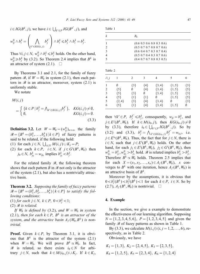
Table 1

k Bk

1 (0.6 0.5 0.6 0.8 0.3 0.6)2 (0.5 0.7 0.7 0.8 0.7 0.6)3 (0.6 0.4 0.7 0.3 0.7 0.4)4 (0.5 0.7 0.4 0.3 0.7 0.6)5 (0.4 0.7 0.7 0.8 0.3 0.5)

Table 2

i\ j 1 2 3 4 5 6

1 ∅ {3} {4} {3; 4} {1; 5} {3}2 {5} ∅ {4} {3; 4} {1; 5} {5}3 {5} {3} ∅ {3; 4} {1; 5} {3}4 {5} {1} {1} ∅ {1; 5} {5}5 {2; 4} {3} {4} {3; 4} ∅ {3}6 {5} {1} {4} {3; 4} {1; 5} ∅

then ∀k ′ ∈P; bk′j 6bkj ; consequently, wjj = bkj ; andj∈Ej(Bk;W0): If k ∈M (i0; j); then KG(i0; j) 6= ∅by (3:3); therefore i0 ∈

⋃k′∈P IG(B

k′ ; j): So by(3.2) and (3.3), bkj =

∧k′∈KG(i0 ; j) b

k′j =wi0j; i.e.

j∈Ei0 (Bk;W0): Thus, the fact that for j∈N; there isi∈N; such that j∈Ei(Bk;W0) holds. On the otherhand, for each j1 ∈Ei(Bk;W0); j2 ∈Gi(Bk;W0); thenw0ij1 = b

kj1 ; w

0ij2¿b

kj2 hold.B is related implies bkj2¿b

kj1 :

Therefore Bk ∝W0 holds. Theorem 2.5 implies thatfor each X =(x1; x2; : : : ; xn)∈Af (Bk;W0); x con-verges to Bk with one iteration, hence Af (Bk;W0) isan attractive basin of Bk:Moreover by the assumptions, it is obvious that

0¡b1i (Bk)¡b2i (B

k)¡1 for each k ∈P; i∈N: So by(2.7), Af (Bk;W0) is nontrivial.

4. Example

In the section, we give a example to demonstratethe e�ectiveness of our learning algorithm. SupposingN = {1; 2; 3; 4; 5; 6}; P= {1; 2; 3; 4; 5} and given thefamily B of fuzzy patterns as shown in Table 1.By (3.3), we calculateM (i; j) (i; j=1; 2; : : : ; 6), re-

spectively, as in Table 2.Obviously, we have

K1 = {1; 3}; K2 = {2; 4; 5}; K3 = {2; 3; 5};K4 = {1; 2; 5}; K5 = {2; 3; 4}; K6 = {1; 2; 4}


Table 3Values of b1i (B

k)

i\k 1 2 3 4 5

1 0.6 0 0.6 0.4 0.32 0.3 0.7 0.3 0.7 0.73 0.3 0.7 0.7 0.3 0.74 0.8 0.8 0 0 0.85 0 0.7 0.7 0.7 06 0.6 0.6 0.3 0.6 0.4

Table 4Values of b2i (B

k)

i\k 1 2 3 4 5

1 1 0.5 1 0.5 0.42 0.5 1 0.4 1 13 0.6 1 1 0.4 14 1 1 0.3 0.3 15 0.3 1 1 1 0.36 1 1 0.4 1 0.5

which imply ∀j∈N; ⋃i∈N M (i; j)∪Kj =P: More-over, we calculate W0 = (w0ij)6×6 by (3.2) as follows:

W0 =

0:6 0:4 0:4 0:3 0:3 0:40:4 0:7 0:4 0:3 0:3 0:50:4 0:4 0:7 0:3 0:3 0:40:4 0:5 0:6 0:8 0:3 0:50:5 0:4 0:4 0:3 0:7 0:40:4 0:5 0:4 0:3 0:3 0:6

:

It is easy to prove that the family B is related. ByTheorem 3.2, if we let W =W0 de�ned by (3.2) insystem (2.1), then all B1; B2; : : : ; B5 are the attractorsof the system. Therefore with (2.7), we can calculatethe attractive basins of the pattern Bk (k ∈P), respec-tively. At �rst, we have Tables 3 and 4 about b1i (B

k)and b2i (B

k) by (2.6).To calculate Af (Bk;W0) (k ∈P); we now derive

GE(Bk;W0); G(Bk;W0); E(Bk;W0); and L(Bk;W0), re-spectively, for k ∈P as shown in Table 5.So we obtain the attractive basins as follows by

(2.7).

Af (B1; W0) = [0:6; 1]× [0:3; 0:5]× [0:3; 0:6]× [0:8; 1]× [0; 0:3]× [0:6; 1];

Table 5

k GE(Bk ; W0) E(Bk ; W0) G(Bk ; W0) L(Bk ; W0)

1 {2; 3} {1; 4; 6} {5} ∅2 ∅ {2; 3; 4; 5; 6} {1} ∅3 {2; 6} {1; 3; 5} {4} ∅4 {1; 3} {2; 5; 6} {4} ∅5 {1; 6} {2; 3; 4} {5} ∅

Af (B2; W0) = [0; 0:5]× [0:7; 1]× [0:7; 1]× [0:8; 1]× [0:7; 1]× [0:6; 1];

Af (B3; W0) = [0:6; 1]× [0:3; 0:4]× [0:7; 1]× [0; 0:3]× [0:7; 1]× [0:3; 0:4];

Af (B4; W0) = [0:4; 0:5]× [0:7; 1]× [0:3; 0:4]× [0; 0:3]× [0:7; 1]× [0:6; 1];

Af (B5; W0) = [0:3; 0:4]× [0:7; 1]× [0:7; 1]× [0:8; 1]× [0; 0:3]× [0:4; 0:5]:

5. Conclusion

In the paper, we obtain the facts that the max–minfuzzy Hop�eld networks are Lyapunov stable, and theabilities of storage of the networks are very strong.With some conditions for the connected weight ma-trix, the networks have good fault-tolerance, and areuniformly stable. These conclusions are demonstratedby our numerical example. It is noteworthy that thelearning algorithms for the weight matrix W are de-signed such that the attractive basins of the attractorsare as large as possible. The problem is left for futurestudies.

References

[1] A. Blanco, M. Delgado, I. Requena, Identi�cation of relationalequations by fuzzy neural networks, Fuzzy Sets and Systems71 (1995) 215–226.

[2] A. Blanco, M. Delgado, I. Requena, Improved fuzzy neuralnetworks for solving relational equations, Fuzzy Sets andSystems 72 (1995) 311–322.

[3] J.J. Buckley, Y. Hayashi, Fuzzy neural networks: a survey,Fuzzy Sets and Systems 66 (1994) 1–13.

[4] F.L. Chung, T. Lee, On fuzzy associative memory withmultiple-rule storage capacity, IEEE Trans. Fuzzy Systems 4(1996) 375–384.


[5] J.B. Fan, F. Jin, Y. Shi, An e�cient learning algorithm forfuzzy associative memories, Acta Elect. Sinica 24 (1996)112–114.

[6] H. Ishibuchi, K. Kwon, H. Tanaka, A learning algorithm offuzzy neural networks with triangular fuzzy weights, FuzzySets and Systems 71 (1995) 277–293.

[7] B. Kosko, Fuzzy associative memories, in: A. Kandel (Ed.),Fuzzy Expert Systems Reading, Addison-Wesley, Reading,MA, 1987.

[8] S.C. Lee, E.T. Lee, Fuzzy neural networks, Math. Biosci. 23(1975) 151–177.

[9] W. Pedrycz, Fuzzy neural networks and neurocomputations,Fuzzy Sets and Systems 56 (1993) 1–28.

[10] E. Sanchez, Eigen fuzzy sets and fuzzy relations, J. Math.Anal. Appl. 81 (1981) 399–421.

[11] E. Sanchez, Eigen fuzzy sets, Session approximate reasoningand approximate algorithms in computer science, NNC,New York, June 7–10, 1976.

[12] P.K. Simpson, Fuzzy min–max neural networks-part 1:classi�cation, IEEE Trans. Neural Networks 3 (1992)777–786.

[13] P.K. Simpson, Fuzzy min–max neural networks – part 2:clustering, IEEE Trans. Fuzzy Systems 1 (1993) 32–45.

[14] Z.F. Wang, D.M. Jin, Z.J. Li, Research on monolithic fuzzyneural networks self-learning problems, Acta Elect. Sinica 25(1997) 33–38.

[15] X.H. Zhang, C.C. Hang, S.H. Tan, P.Z. Wang, The Min–maxfunction di�erentation and training of fuzzy neural networks,IEEE Trans. Neural Networks 7 (1996) 1139–1150.

max–min fuzzy hopfield neural networks and an efficient learning algorithm

Documents