May 2007May 2007 Hua Fan University, TaipeiHua Fan University, Taipei

An Introductory Talk on Reliability An Introductory Talk on Reliability AnalysisAnalysis

With contribution from Yung Chia HSUWith contribution from Yung Chia HSU

Jeen-Shang Lin

University of Pittsburgh

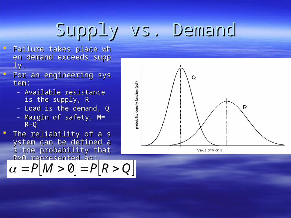
Supply vs. DemandSupply vs. Demand Failure takes place when dFailure takes place when d

emand exceeds supply.emand exceeds supply. For an engineering system:For an engineering system:

– Available resistance is the Available resistance is the supply, Rsupply, R

– Load is the demand, QLoad is the demand, Q– Margin of safety, M=R-QMargin of safety, M=R-Q

The reliability of a system The reliability of a system can be defined as the probcan be defined as the probability that R>Q representeability that R>Q represented asd as: :

QRPMP 0

RiskRisk

The probability of failure, or riskThe probability of failure, or risk

1)0(1)0( MPMPpF

How to find the risk?How to find the risk?– If we known the distribution of M;If we known the distribution of M;– or, the mean and variance of M;or, the mean and variance of M;– then we can compute P(M<0) easily.then we can compute P(M<0) easily.

Normal distribution: the bell curveNormal distribution: the bell curve

10

))(

(2

1)(

2

2

x

exf

For a wide variety of conditions, the distribution of the sum of a large number of random variables converge to Normal distribution. (Central Limit Theorem)

x xexF )

)((

2

1)(

2

2

IF M=Q-R is normalIF M=Q-R is normal

)()(2

1)

)((

2

1)( 2

2

2

xxex

exFxx

)()0(M

MF MPp

10 When

Because of symmetryBecause of symmetry)(1)( xx )(1

M

MFp

Define Define reliability indexreliability indexMM /

Example: vertical cut in clayExample: vertical cut in clay

kPacc 30100

4/HcM

3/220 mkN

5.0c

If all variables are normal,If all variables are normal,

21062.3796.183.2750 FMM p

10H

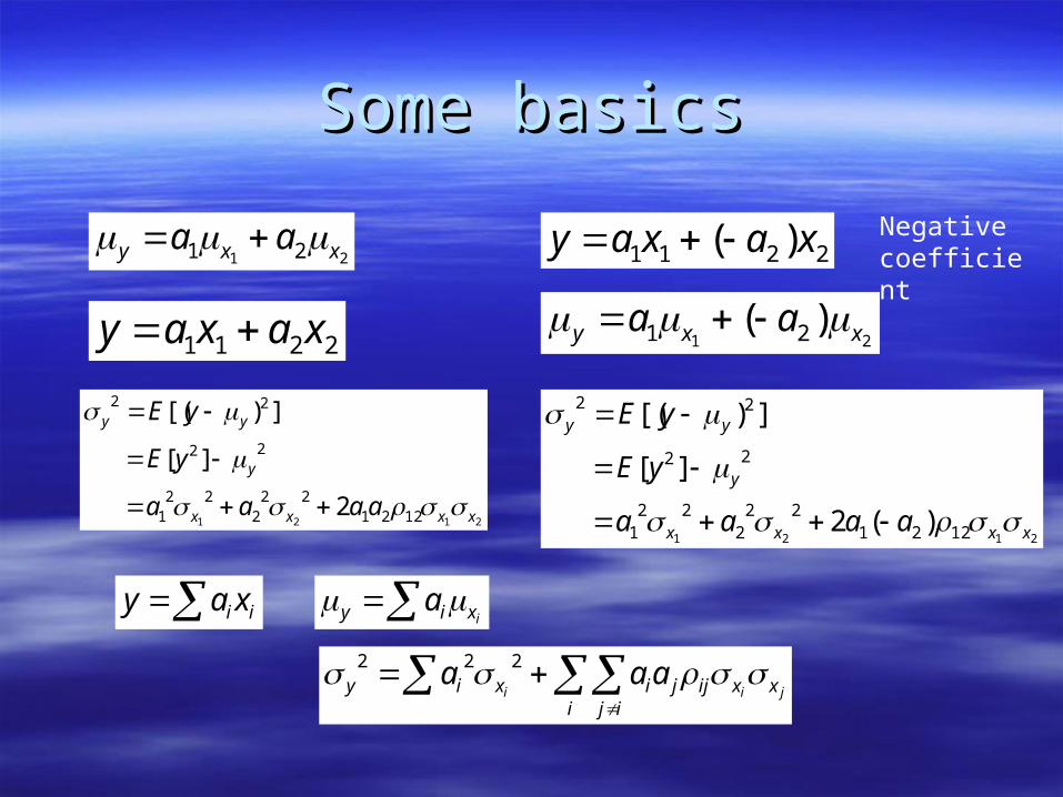
Some basicsSome basics

21 21 xxy aa

iixay

2121 122122

222

1

22

22

2

][

])[(

xxxx

y

yy

aaaa

yE

yE

21)( 21 xxy aa

2211 )( xaxay

2121 122122

222

1

22

22

)(2

][

])[(

xxxx

y

yy

aaaa

yE

yE

Negative coefficient

2211 xaxay

ixiy a

jii xxijji ij

ixiy aaa

222

Engineers like Factor of safetyEngineers like Factor of safety

F=R/Q, if F is normal F=R/Q, if F is normal

)(1)1

()1(

F

FF FPp

reliability indexreliability indexF

F

1

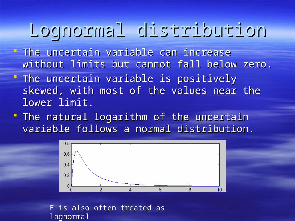
Lognormal distributionLognormal distribution The uncertain variable can increase without The uncertain variable can increase without

limits but cannot fall below zero. limits but cannot fall below zero. The uncertain variable is positively skewed, with The uncertain variable is positively skewed, with

most of the values near the lower limit. most of the values near the lower limit. The natural logarithm of the uncertain variable The natural logarithm of the uncertain variable

follows a normal distribution. follows a normal distribution.

F is also often treated as lognormal

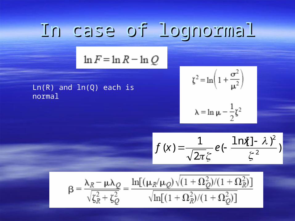
In case of lognormalIn case of lognormal

))]ln[

(2

1)(

2

2

x

exf

Ln(R) and ln(Q) each is normal

The MFOSM method assumes that the unceThe MFOSM method assumes that the uncertainty features of a random variable can be rtainty features of a random variable can be represented by its first two moments: mean represented by its first two moments: mean and variance. and variance.

This method is based on the Taylor series eThis method is based on the Taylor series expansion of the performance function linearixpansion of the performance function linearized at the mean values of the random variazed at the mean values of the random variables. bles.

First order second moment methodFirst order second moment method

First order second moment methodFirst order second moment method

Taylor series Taylor series expansionexpansion

),.....,( 21 nxxxgg dx

dgXxXgg )()(

i

xiixnxxn x

gxgxxxg )(),...,,(),...,,( 2121

),...,,( 21 xnxxg g

i ji ji

xjxixixji

xigx

g

x

g

x

g 2

22

Example: vertical cut in clayExample: vertical cut in clay

kPacc 30100 H

cF

4

3/220 mkN

5.0c

If all variables are normal,If all variables are normal,

21094.28896.15292.02 FFF p

10H

Hc

F

4

H

cF2

4

F

F

1

1-normcdf(1.8896,0,1) MATLAB

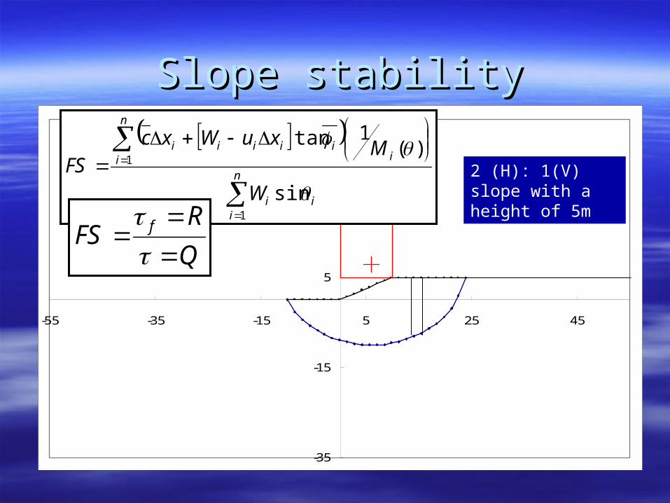
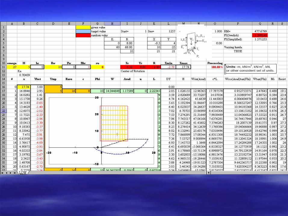
Slope stabilitySlope stability

-35

-15

5

25

-55 -35 -15 5 25 45

n

iii

n

i iiiiii

W

MxuWxcFS

1

1

sin

)(1tan

Q

RFS f

2 (H): 1(V) slope with a height of 5m

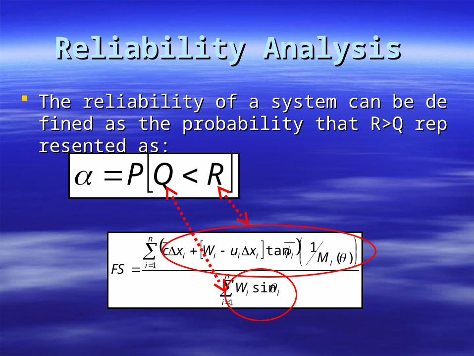
Reliability AnalysisReliability Analysis

The reliability of a system can be defined as the pThe reliability of a system can be defined as the probability that R>Q represented asrobability that R>Q represented as: :

RQP

n

iii

n

i iiiiii

W

MxuWxcFS

1

1

sin

)(1tan

kPacc 210

210

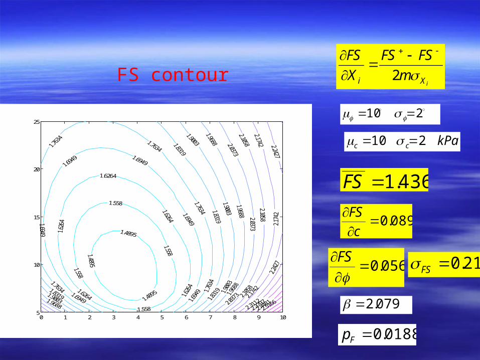
0188.0Fp0 1 2 3 4 5 6 7 8 9 10

5

10

15

20

25

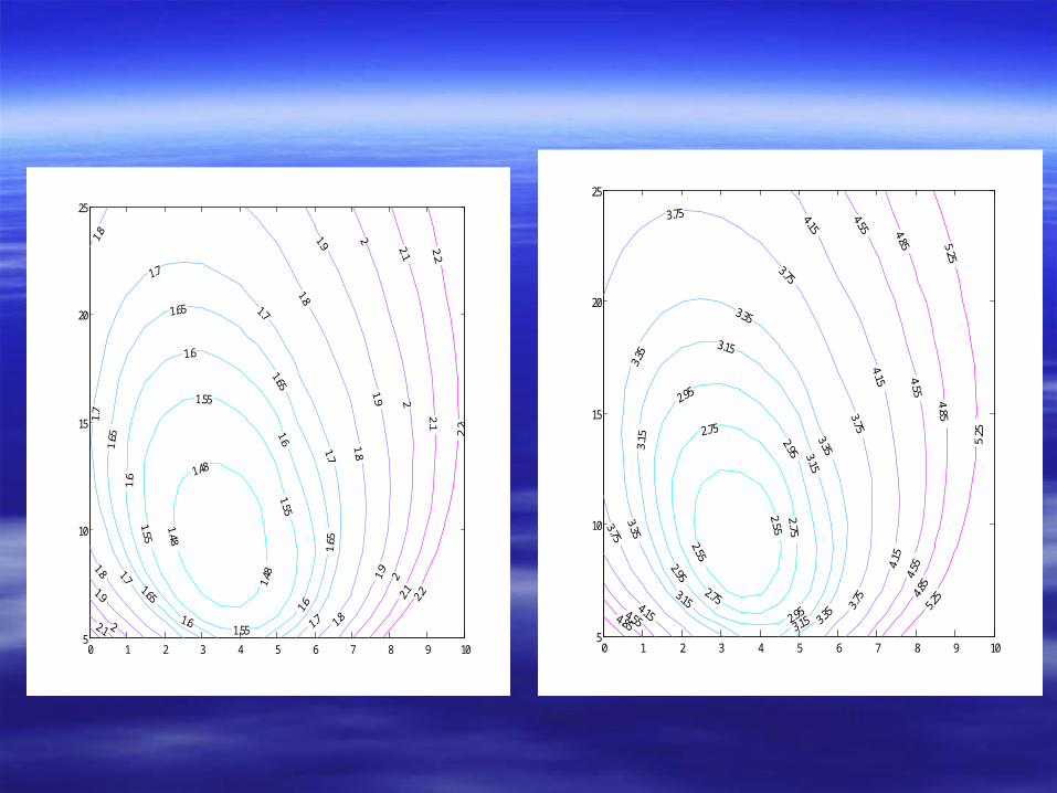
FS contouriXi m

FSFS

X

FS

2

436.1FS

089.0

c

FS

056.0

FS 21.0FS

,

,

0.21.

079.2

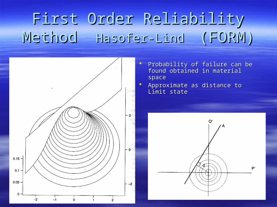
First Order Reliability Method First Order Reliability Method Hasofer-Lind Hasofer-Lind (FORM)(FORM)

Probability of failure can be found Probability of failure can be found obtained in material spaceobtained in material space

Approximate as distance to Limit Approximate as distance to Limit statestate

Distance to failure criterion Distance to failure criterion

If F=1 or M=0 is a straight lineIf F=1 or M=0 is a straight line Reliability becomes the shortest Reliability becomes the shortest

distancedistance

Constraint Optimization:ExcelConstraint Optimization:Excel

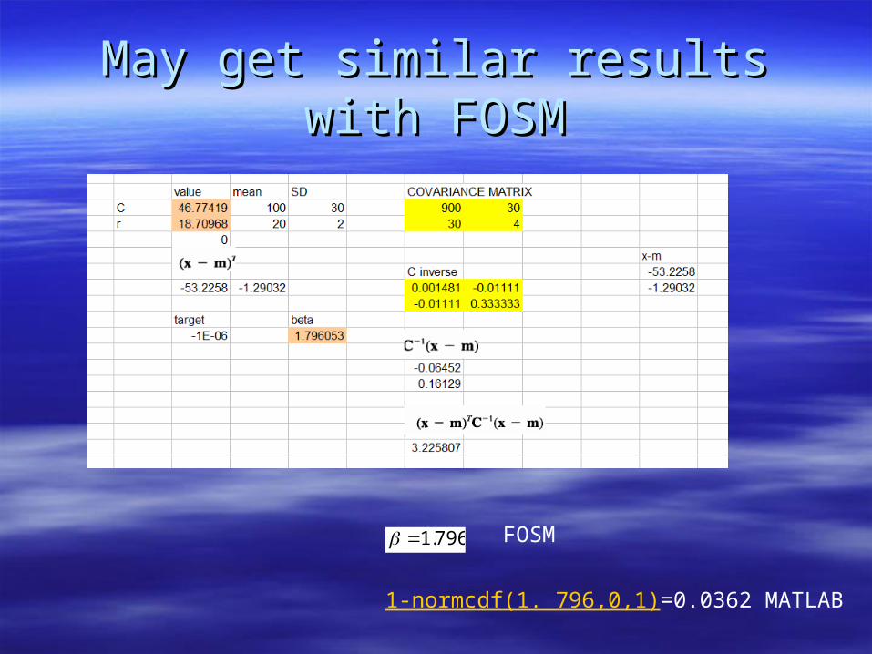
May get similar results with FOSMMay get similar results with FOSM

796.1 FOSM

1-normcdf(1. 796,0,1)=0.0362 MATLAB

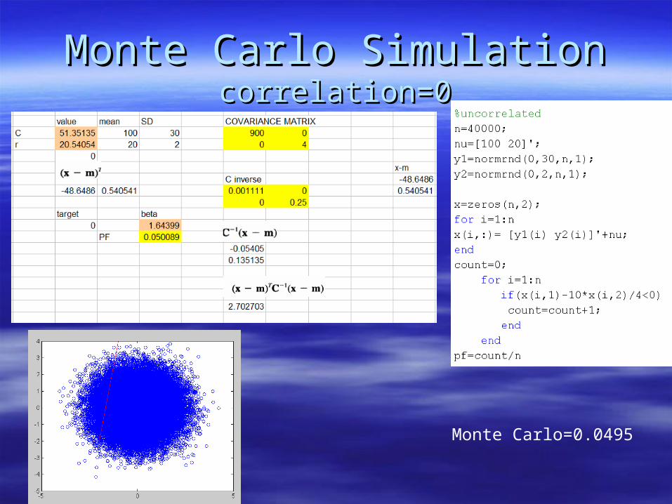
Monte Carlo SimulationMonte Carlo Simulationcorrelation=0correlation=0

Monte Carlo=0.0495

Monte Carlo SimulationMonte Carlo Simulationcorrelation=0.5correlation=0.5

FORM=0.0362

}{][][}{ 21 *T/Y

* XTCY

2/12/1

2/12/1][T

10

01][ YC

-5

-4

-3

-2

-1

0

1

2

3

-5 -4 -3 -2 -1 0 1 2 3 4 5

Mean

Mean + - S.D.

FS=1.436

FS=1.0

FS=1.259

FS=1.324

FS=1.549

FS=1.613

c

ccc

*

*

xy 2

1

)XX(C)XX( 1X

Xmin

T

stateLimit

c

cc

FS=1.0 (M=0)

UNSAFE

Region

FS<1 or M<0

The matrix form of the

Hasofer-Lind (1974)

The matrix form of the

Hasofer-Lind (1974)

FOS=1Soil properties>0

Soil properties

0 1 2 3 4 5 6 7 8 9 105

10

15

20

25

1.55

0 1 2 3 4 5 6 7 8 9 105

10

15

20

25

cc

c

FS=1.0

UNSAFE

Region

FS<1 or

M<0Correlation=0

Correlation=-.99

Correlation=.99

The distanceThe distance

unsaferegion

c*

*

c

ccc

*

)0,0( ** c

*FS

*cFS

*

1

c

FS

FS/),( ** c

2222

22

)/()/(

1)()( **

FScFS

FSc

c

FOSM maybe wrongFOSM maybe wrong

FOSMFOSM

2

1

X

YSoil 1

Soil 2

c1

c22

9.10 m

6.14 m

A projection MethodA projection Method

Check the FOSMCheck the FOSM Use the slope, projected to where the Use the slope, projected to where the

failure material isfailure material is Use the material to find FSUse the material to find FS If FS=1, okIf FS=1, ok

n

iXi

Xiipi

i

I

XFS

XFSFSXx

1

22

2

)/(

)/)(1()(

May 2007May 2007 Hua Fan University, TaipeiHua Fan University, Taipei