mcfor: a matlab to fortran 95 · pdf fileinterpreter, leads to poor ... the mcfor compiler...
TRANSCRIPT
MCFOR: A MATLAB TO FORTRAN 95 COMPILER
by
Jun Li
School of Computer Science
McGill University, Montreal
Auguest 2009
a thesis submitted to the Faculty of Graduate Studies and Research
in partial fulfillment of the requirements for the degree of
Master of Science
Copyright c© 2010 by Jun Li


Abstract
The high-level array programming language MATLAB is widely used for prototyp-
ing algorithms and applications of scientific computations. However, its dynamically-
typed nature, which means that MATLAB programs are usually executed via an
interpreter, leads to poor performance. An alternative approach would be converting
MATLAB programs to equivalent Fortran 95 programs. The resulting programs could
be compiled using existing high-performance Fortran compilers and thus could pro-
vide better performance. This thesis presents techniques that are developed for our
MATLAB-to-Fortran compiler, McFor, for extracting information from the high-level
semantics of MATLAB programs to produce efficient and reusable Fortran code.
The McFor compiler includes new type inference techniques for inferring intrinsic
type and shape of variables and uses a value-propagation analysis to precisely estimate
the sizes of arrays and to eliminate unnecessary array bounds checks and dynamic
reallocations. In addition to the techniques for reducing execution overhead, McFor
also aims to produce programmer-friendly Fortran code. By utilizing Fortran 95 fea-
tures, the compiler generates Fortran code that keeps the original program structure
and preserves the same function declarations.
We implemented the McFor system and experimented with a set of benchmarks
with different kinds of computations. The results show that the compiled Fortran
programs perform better than corresponding MATLAB executions, with speedups
ranging from 1.16 to 102, depending on the characteristics of the program.
i

ii
Resum e
Le langage de programmation de tableaux de haut niveau MATLAB est large-
ment utilise afin de faire du prototypage d’algorithmes et des applications de calculs
scientifiques. Cependant, sa nature de type dynamique, ce qui veut dire que les pro-
grammes MATLAB sont habituellement executes par un interpreteur, amene une
mauvaise performance. Une approche alternative serait de convertir les programmes
MATLAB aux programmes Fortran 95 equivalents. Les programmes resultants pour-
raient etre compiles en utilisant les compilateurs de haute performance Fortran, ainsi
ils peuvent fournir une meilleure performance. Cette these presente les techniques qui
sont developpees pour notre compilateur MATLAB-a-Fortran, McFor, pour extraire
l’information des hauts niveaux des semantiques des programmes MATLAB afin de
produire un code Fortran efficace et reutilisable.
Le compilateur McFor inclut de nouvelles techniques de deduction pour inferer
les types et formes intrinseques des variables et utilise une analyse a propagation
de valeurs pour estimer avec precision la tailles des tableaux de variables et pour
eliminer les verifications des limites et les reallocations dynamiques superflues de
ces tableaux. En plus de ces techniques de reduction des temps d’execution, McFor
vise aussi a generer du code Fortran convivial pour les developpeurs. En utilisant
les avantages de Fortran 95, le compilateur genere du code Fortran qui preserve la
structure originale du programme ainsi que les memes declarations de fonctions.
Nous avons mis en oeuvre le systeme McFor et l’avons experimente avec un
ensemble de tests de performance avec differentes sortes de calculs. Les resultats
montrent que les programmes de Fortran compiles offrent une meilleure performance
que les executions MATLAB correspondantes, avec une cadence acceleree de l’ordre
iii

de 1.16 a 102, selon les caracteristiques du programme.
iv
Acknowledgements
I would like to thank my supervisor, Professor Laurie Hendren, for her continual
support, guidance, assistance, and encouragement throughout the research and the
writing of this thesis. This thesis would not have been possible without her support.
I would also like to thank my fellow students of McLab team and Sable research
group for their constructive discussions, valuable comments and suggestions that have
greatly improved this work. In particular, I would like to thank Anton Dubrau for
providing very useful comments on the compiler and extending its features, Alexandru
Ciobanu for implementing the aggregation transformation.
Finally, I am grateful to my parents and my wife for their love and support
throughout my study.
v

vi
Table of Contents
Abstract i
Resume iii
Acknowledgements v
Table of Contents vii
List of Figures xi
List of Tables xiii
List of Listings xv
List of Listings xv
1 Introduction 1
1.1 Introduction . . . . . . . . . . . . . . . . . . . . . . . . . . . . . . . . 1
1.2 Thesis Contributions . . . . . . . . . . . . . . . . . . . . . . . . . . . 2
1.2.1 Shape Inference . . . . . . . . . . . . . . . . . . . . . . . . . . 2
1.2.2 Generate Readable and Reusable Code . . . . . . . . . . . . . 3
1.2.3 Design and Implementation of the McFor Compiler . . . . . . 3
1.3 Organization of Thesis . . . . . . . . . . . . . . . . . . . . . . . . . . 4
2 Related Work 5
2.1 The MATLAB Language . . . . . . . . . . . . . . . . . . . . . . . . . 5
vii
2.1.1 Language Syntax and Data Structure . . . . . . . . . . . . . . 5
2.1.2 MATLAB’s Type System . . . . . . . . . . . . . . . . . . . . . 6
2.1.3 The Structure of MATLAB programs . . . . . . . . . . . . . . 6
2.2 FALCON Project . . . . . . . . . . . . . . . . . . . . . . . . . . . . . 8
2.3 MATLAB Compilers . . . . . . . . . . . . . . . . . . . . . . . . . . . 10
2.4 Parallel MATLAB Compilers . . . . . . . . . . . . . . . . . . . . . . 12
2.5 Vectorization of MATLAB . . . . . . . . . . . . . . . . . . . . . . . . 12
2.6 Other MATLAB Projects . . . . . . . . . . . . . . . . . . . . . . . . 13
2.7 Summary of McFor’s Approach . . . . . . . . . . . . . . . . . . . . . 14
3 Overview of the McFor Compiler 15
3.1 Structure of the Compiler . . . . . . . . . . . . . . . . . . . . . . . . 16
3.1.1 MATLAB-to-Natlab Translator . . . . . . . . . . . . . . . . . 16
3.1.2 Lexer and Parser . . . . . . . . . . . . . . . . . . . . . . . . . 16
3.1.3 Analyses and Transformations . . . . . . . . . . . . . . . . . . 18
3.1.4 Code Generator . . . . . . . . . . . . . . . . . . . . . . . . . . 18
3.2 Preparation Phase . . . . . . . . . . . . . . . . . . . . . . . . . . . . 19
3.2.1 Inlining Script M-files . . . . . . . . . . . . . . . . . . . . . . 20
3.2.2 Distinguishing Function Calls from Variables . . . . . . . . . . 21
3.2.3 Simplification Transformation . . . . . . . . . . . . . . . . . . 23
3.2.4 Renaming Loop-Variables . . . . . . . . . . . . . . . . . . . . 25
3.2.5 Building the Symbol Table . . . . . . . . . . . . . . . . . . . . 26
4 Type Inference Mechanism 29
4.1 Type Inference Principles . . . . . . . . . . . . . . . . . . . . . . . . . 29
4.1.1 Intrinsic Type Inference . . . . . . . . . . . . . . . . . . . . . 29
4.1.2 Sources of Type Inference . . . . . . . . . . . . . . . . . . . . 31
4.1.3 Shape Inference . . . . . . . . . . . . . . . . . . . . . . . . . . 34
4.2 Type Inference Process . . . . . . . . . . . . . . . . . . . . . . . . . . 35
4.2.1 Function Type Signature . . . . . . . . . . . . . . . . . . . . . 35
4.2.2 Whole-Program Type Inference . . . . . . . . . . . . . . . . . 36
viii
4.2.3 The Type Inference Algorithm . . . . . . . . . . . . . . . . . . 37
4.3 Intermediate Representation and Type Conflict Functions . . . . . . . 38
4.3.1 Disadvantages of SSA Form in Type Inference . . . . . . . . . 39
4.3.2 Type Conflict Functions . . . . . . . . . . . . . . . . . . . . . 40
4.4 Solving Type Differences . . . . . . . . . . . . . . . . . . . . . . . . . 41
4.4.1 Merging Intrinsic Types . . . . . . . . . . . . . . . . . . . . . 42
4.4.2 Solving Differences Between Shapes . . . . . . . . . . . . . . . 43
4.5 Type Inference on Type Conflict Functions . . . . . . . . . . . . . . . 45
4.5.1 Type Inference on Apha-functions . . . . . . . . . . . . . . . . 46
4.5.2 Type Inference on Beta-functions . . . . . . . . . . . . . . . . 46
4.5.3 Type Inference on Lambda-functions . . . . . . . . . . . . . . 48
4.6 Value Propagation Analysis . . . . . . . . . . . . . . . . . . . . . . . 48
4.6.1 Calculate a Variable’s Value . . . . . . . . . . . . . . . . . . . 49
4.6.2 Compare Values . . . . . . . . . . . . . . . . . . . . . . . . . . 50
4.6.3 Additional Rule for Array Bounds Checking . . . . . . . . . . 50
4.7 Determine the Shape at Runtime . . . . . . . . . . . . . . . . . . . . 52
4.7.1 Determine the Shape at Runtime . . . . . . . . . . . . . . . . 52
4.7.2 Checking Array Bounds and Resizing Array at Runtime . . . 55
4.8 Other Analyses in the Type Inference Process . . . . . . . . . . . . . 55
4.8.1 Discover Identifiers That are not Variables . . . . . . . . . . . 57
4.8.2 Discover the Basic Imaginary Unit of Complex Numbers . . . 57
5 Transformations 59
5.1 Transformations for Array Constructions . . . . . . . . . . . . . . . . 59
5.2 Transformations for Linear Indexing . . . . . . . . . . . . . . . . . . . 61
5.3 Transformations for Using Arrays as Indices . . . . . . . . . . . . . . 63
5.4 Transformations for Type Conversions . . . . . . . . . . . . . . . . . 65
5.4.1 Logical and Character Type in Computations . . . . . . . . . 65
5.4.2 Fortran’s Limited Type Conversions . . . . . . . . . . . . . . . 66
5.5 Aggregation Transformation . . . . . . . . . . . . . . . . . . . . . . . 68
ix
6 Performance Evaluation 71
6.1 Description of the Benchmarks . . . . . . . . . . . . . . . . . . . . . . 71
6.2 Performance Results . . . . . . . . . . . . . . . . . . . . . . . . . . . 73
6.3 Comparison of Compiled Fortran Code to MATLAB . . . . . . . . . 74
6.4 Comparison of Dynamic Reallocation in Fortran and MATLAB . . . 79
6.4.1 Dynamic Reallocation Tests . . . . . . . . . . . . . . . . . . . 79
6.4.2 Different Reallocation Strategies Tests . . . . . . . . . . . . . 81
6.4.3 Overhead of Passing Dynamically Allocatable Arrays . . . . . 83
6.5 Summary of Fortran 95 vs. MATLAB . . . . . . . . . . . . . . . . . . 84
6.6 Comparison of Compiled Fortran Code to Octave . . . . . . . . . . . 84
6.7 Comparison of Compiled Fortran Code to McVM . . . . . . . . . . . 85
7 Conclusions and Future Work 87
7.1 Conclusions . . . . . . . . . . . . . . . . . . . . . . . . . . . . . . . . 87
7.2 Future Work . . . . . . . . . . . . . . . . . . . . . . . . . . . . . . . . 88
Appendices
A Supported MATLAB Features 91
Bibliography 93
x
List of Figures
3.1 McFor Compiler Structure with Analyses and Transformations . . . . 17
4.1 The Intrinsic Type Lattice.(similar to the lattice used in [JB01]) . . . 30
6.1 Speedup of McFor over MATLAB . . . . . . . . . . . . . . . . . . . . 76
6.2 Speedup of McFor over MATLAB on different reallocation sizes (1) . 80
6.3 Speedup of McFor over MATLAB on different reallocation sizes (2) . 80
6.4 Speedup of McFor over MATLAB on different reallocation sizes (3) . 81
6.5 Number of reallocations of different expanding factor . . . . . . . . . 82
6.6 Speedup over MATLAB on different expanding factor . . . . . . . . . 82
xi

xii
List of Tables
3.1 Computing mean of a matrix by script and function . . . . . . . . . . 20
3.2 Variables are determined at runtime . . . . . . . . . . . . . . . . . . . 23
3.3 Simplify long expression . . . . . . . . . . . . . . . . . . . . . . . . . 26
3.4 Loop variable changes are kept inside the iteration . . . . . . . . . . . 26
4.1 The result of type functions for operator “+”. . . . . . . . . . . . . . 32
4.2 The result of type functions for operators “^”, “.^”. . . . . . . . . . . 32
4.3 The result of type functions for operator “:”. . . . . . . . . . . . . . 32
4.4 Three ways to dynamically change a variable’s shape . . . . . . . . . 34
4.5 Type conflict function example . . . . . . . . . . . . . . . . . . . . . 41
4.6 Type inference example. . . . . . . . . . . . . . . . . . . . . . . . . . 42
4.7 Converting array concatenation. . . . . . . . . . . . . . . . . . . . . . 44
4.8 A code segment with alpha-function . . . . . . . . . . . . . . . . . . . 46
4.9 A code segment with lambda-function . . . . . . . . . . . . . . . . . . 47
4.10 Value-propagation analysis example 1. . . . . . . . . . . . . . . . . . 51
4.11 Value-propagation analysis example 2 . . . . . . . . . . . . . . . . . . 52
5.1 MATLAB array construction and concatenation expressions . . . . . 60
5.2 Example of using a logical array as an index . . . . . . . . . . . . . . 65
5.3 Example of using an integer array as an index . . . . . . . . . . . . . 66
5.4 Converting logical and character type variables . . . . . . . . . . . . . 67
5.5 Type conversion example 2 . . . . . . . . . . . . . . . . . . . . . . . . 68
6.1 Benchmarks’ execution times (in seconds). . . . . . . . . . . . . . . . 75
6.2 Speedup over MATLAB execution . . . . . . . . . . . . . . . . . . . . 75
xiii

xiv
List of Listings
2.1 Example of a MATLAB function . . . . . . . . . . . . . . . . . . . . 7
2.2 Example of a MATLAB script . . . . . . . . . . . . . . . . . . . . . . 8
4.1 Example of unpredictable array shape . . . . . . . . . . . . . . . . . . 53
4.2 Fortran code for handling array shape at runtime . . . . . . . . . . . 54
4.3 MATLAB code segment for array bounds checking and resizing . . . 55
4.4 Fortran code segment for array bounds checking and resizing . . . . . 56
4.5 The meaning of i, j depends on context . . . . . . . . . . . . . . . . . 58
5.1 MATLAB code segment of linear indexing . . . . . . . . . . . . . . . 62
5.2 Transformed code segment of linear indexing . . . . . . . . . . . . . . 62
5.3 Example of using arrays as indices . . . . . . . . . . . . . . . . . . . . 64
5.4 Transformed code segment of using arrays as indices . . . . . . . . . . 64
5.5 Example of the Aggregation transformation . . . . . . . . . . . . . . 69
6.1 Passing array with or without its size. . . . . . . . . . . . . . . . . . . 84
xv

xvi
Chapter 1
Introduction
1.1 Introduction
MATLAB R©1 is a popular scientific computing system and array programming lan-
guage. The MATLAB language offers high-level matrix operators and an extensive
set of built-in functions that enable developers to perform complex mathematical
computations from relatively simple instructions. Because of the interpreted nature
of the language and the easy-to-use interactive development environment, MATLAB
is widely used by scientists of many domains for prototyping algorithms and applica-
tions.
The MATLAB language is weakly typed; it does not have explicit type declara-
tions. A variable’s type is implicit from the semantics of its operations and the type
is allowed to dynamically change at runtime. These features raise the language’s level
of abstraction and improve ease of use, but add heavy overheads, such as runtime
type and shape checking, array bounds checking and dynamic resizing, to its inter-
pretive execution. Therefore, MATLAB programs often run much slower than their
counterparts that are written in conventional program languages, such as Fortran.
Fortran programs have other advantages over MATLAB programs. They can be
well integrated with most of the linear algebra libraries, such as BLAS and LAPACK
1MATLAB is a registered trademark of the MathWorks, Inc.
1
Introduction
[ABB+99], which are written in Fortran and used by MATLAB for performing matrix
computations. There are many Fortran parallel compilers that can further optimize
Fortran programs to improve their performance in parallel environments.
Our MATLAB-to-Fortran 95 compiler, McFor, is designed to improve the perfor-
mance of programs and produce readable code for further improvement.
In our McFor compiler, we applied and extended type inference techniques that
were developed in the FALCON [RP99, RP96] and MaJIC [AP02] projects. We used
intrinsic type inference based on the type hierarchy to infer the intrinsic type of all
variables [JB01]. We developed a value propagation analysis associated with our
shape inference to estimate the sizes of the array variables and precisely discover the
statements that need array bounds checks and dynamic reallocations.
We also created several special transformations to support features specific to
MATLAB, such as array concatenations, linear indexing and using arrays as indices.
We utilized the Fortran 95 enhanced features of allocatable arrays to construct the
Fortran code, which preserves the same program structure and function declarations
as in the original MATLAB program.
1.2 Thesis Contributions
In creating the McFor compiler, we have explored the language differences and perfor-
mance differences between MATLAB (version 7.6) and Fortran 95. We have designed
our new approach around two key features: precisely inferring the array shape; and
generating readable and reusable code.
We have built upon ideas from previous projects, such as FALCON and MaJIC.
These previous systems are described in Chapter 2.
1.2.1 Shape Inference
In the executions of compiled Fortran programs, array bounds checking and dynamic
reallocations cause most runtime overheads. In order to generate efficient Fortran
code, our shape inference mechanism aims to infer the array shape as precisely as
2
1.2. Thesis Contributions
possible and eliminate unnecessary array bounds checks.
Our shape inference considers all the cases, where the array shape can be dy-
namically changed (described in Section 4.1.3). We first use a special transformation
to handle the cases where the array shape is changed by array concatenation opera-
tions (described in Section 4.4.2). Then we used a simple value propagation analysis
(described in Section 4.6) to estimate the maximum size of the array, and precisely
discover the array accesses that require array bounds checking and array resizing. As
a result, among all twelve benchmarks, only four benchmarks require array bounds
checking, and only one of them requires dynamic reallocations.
1.2.2 Generate Readable and Reusable Code
We focus on two things to make the code to be more readable and reusable: pre-
serving program structure and keeping the original statements, variable names, and
comments.
In order to preserve the program structure, we translated each user-defined func-
tion into a subroutine, and each subroutine has the same list of parameters as the
original function.
We keep the comments in the programs during the lexing and parsing, and restore
them in the generated Fortran code. We preserve the code structure by translating
MATLAB statements to their closest Fortran statements. We create our own in-
termediate representation instead of using SSA form to avoid the variable renaming
process when converting program to SSA form. We also developed the aggregation
transformation (described in Section 5.5) to remove temporary variables created by
the type inference process and to restore the original statements.
1.2.3 Design and Implementation of the McFor Compiler
The McFor compiler is a part of McLab project2, developed by the Sable research
group3 at McGill University. The design and implementation of the compiler is an
2http://www.sable.mcgill.ca/mclab3http://www.sable.mcgill.ca
3
Introduction
important contribution of this thesis. The McFor compiler uses McLab’s front end,
which includes the MATLAB-to-Natlab translator, the Natlab Lexer which is specified
by using MetaLexer [Cas09], and the Natlab Parser which is generated by using
JastAdd [EH07].
McFor uses an intermediate representation that consists of the AST and type con-
flict functions (described in Section 4.3), which are acquired from a structure-based
flow analysis. The McFor compiler inlines the script M-files, and performs interproce-
dural type inference on the program. The type inference process is an iterative process
that infers the types and shapes of all variables until reaching a fixed point. The Mc-
For compiler also uses a value propagation analysis to precisely estimate the sizes of
arrays and eliminate unnecessary array bounds checks and dynamic reallocations.
McFor transforms the code that implements MATLAB special features into their
equivalent forms, and generates Fortran 95 code using the type information stored in
the symbol table.
1.3 Organization of Thesis
This thesis describes the main techniques developed for the compilation of MATLAB
programs. The rest of the thesis is organized as follows. Chapter 2 presents back-
ground information on the MATLAB language and discusses some related works in
the area of compilation of MATLAB. Chapter 3 presents the structure of the compiler
and the overall strategy of each phase of the compiler. Chapter 4 discusses the type
inference mechanism, including the intermediate representation, value propagation
analysis, and runtime array shape checking and reallocation. Chapter 5 describes
transformations used for supporting special MATLAB features, such as array con-
structions, linear indexing and using arrays as indices. Chapter 6 reports experimen-
tal results on the performance of our compiler on a set of benchmarks. Chapter 7
summarizes the thesis and suggests possible directions for future research. Finally,
Appendix A provides a list of MATLAB features supported by this compiler.
4
Chapter 2
Related Work
There have been many attempts for improving the performance of MATLAB pro-
grams. The approaches include source-level transformations [MP99, BLA07], trans-
lating MATLAB to C++ [Ltd99], C [MHK+00, HNK+00, Joi03a, Inc08], and Fortran
[RP99, RP96], Just-In-Time compilation [AP02], and parallel MATLAB compilers
[QMSZ98, RHB96, MT97]. In this chapter, we discuss some of those approaches.
At the first, we begin with a brief overview of the MATLAB language, and discuss
its language features, type system, and program structure with code examples.
2.1 The MATLAB Language
The MATLAB language is a high level matrix-based programming language. It was
originally created in 1970s for easily accessing matrix computation libraries written
in Fortran. After years of evolving, MATLAT has achieved immense popularity and
acceptance throughout the engineering and scientific community.
2.1.1 Language Syntax and Data Structure
The MATLAB language has the similar data types, operators, flow control state-
ments as conventional programming languages Fotran and C. In MATLAB, the most
5
Related Work
commonly used data types are logical, char, single, double; but MATLAB also sup-
ports a range of signed and unsigned intergers, from int8/uint8 to int64/uint64. In
addition to basic operators, MATLAB has a set of arithmetic operators dedicated to
matrix computations, such as the element-wise matrix multiplication operator “.*”,
the matrix transpose operator “’”, and the matrix left division operator “\”.
MATLAB has a matrix view of data. The most basic data structure in MATLAB
is the matrix, a two-dimensional array. Even a scalar variable is a 1-by-1 matrix.
Column vectors and row vectors are viewed as n-by-1 and 1-by-n matrices respectively;
and strings are matrices of characters. Arrays that have more than two dimensions
are also supported in MATLAB as well.
MATLAB supports Fortran’s array syntax and semantics, and also provides more
convenient operations, including array concatenation, linear indexing, and using ar-
rays as indices.
Besides arrays, MATLAB provides other two container data structures, structures
and cell arrays, which are used for storing elements with different types. Elements in
structures and cell arrays can be accessed by field names and indices respectively.
2.1.2 MATLAB’s Type System
MATLAB is a dynamically-typed language; it lacks explicit type declarations. A
variable’s data type, including its intrinsic type and array shape, is according to the
value assigned to it, and is allowed to dynamically change at execution time.
In MATLAB, operators can take operands with any data type. Each operator has
a set of implicit data type conversion rules for handling different types of operands that
participate the operations and determine the result’s type. Thus, in an assignment
statement, the left-hand side variable’s data type is implicit from the semantics of
the right-hand side expression.
2.1.3 The Structure of MATLAB programs
A MATLAB program can consist of two kinds of files, function M-files and script
M-files. A function M-file is a user-defined function that contains a sequence of
6
2.1. The MATLAB Language
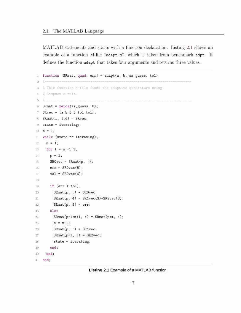
MATLAB statements and starts with a function declaration. Listing 2.1 shows an
example of a function M-file “adapt.m”, which is taken from benchmark adpt. It
defines the function adapt that takes four arguments and returns three values.
1 function [SRmat, quad, err] = adapt(a, b, sz_guess, tol)
2 %-----------------------------------------------------------------------
3 % This function M-file finds the adaptive quadrature using
4 % Simpson’s rule.
5 %-----------------------------------------------------------------------
6 SRmat = zeros(sz_guess, 6);
7 SRvec = [a b S S tol tol];
8 SRmat(1, 1:6) = SRvec;
9 state = iterating;
10 m = 1;
11 while (state == iterating),
12 m = 1;
13 for l = n:-1:1,
14 p = l;
15 SR0vec = SRmat(p, :);
16 err = SR0vec(5);
17 tol = SR0vec(6);
18
19 if (err < tol),
20 SRmat(p, :) = SR0vec;
21 SRmat(p, 4) = SR1vec(3)+SR2vec(3);
22 SRmat(p, 5) = err;
23 else
24 SRmat(p+1:m+1, :) = SRmat(p:m, :);
25 m = m+1;
26 SRmat(p, :) = SR1vec;
27 SRmat(p+1, :) = SR2vec;
28 state = iterating;
29 end;
30 end;
31 end;
Listing 2.1 Example of a MATLAB function
7
Related Work
1 a = -1;
2 b = 6;
3 sz_guess = 1;
4 tol = 4e-13;
5 for i = 1:10
6 [SRmat, quad, err] = adapt(a, b, sz_guess, tol);
7 end
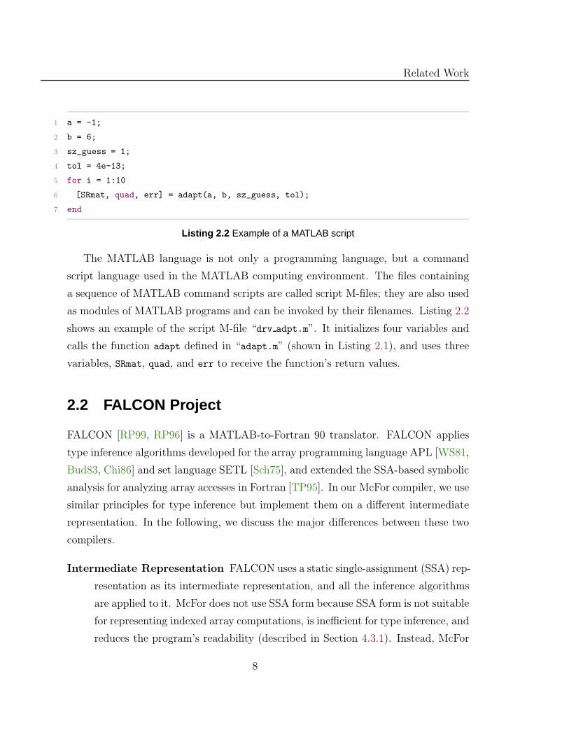
Listing 2.2 Example of a MATLAB script
The MATLAB language is not only a programming language, but a command
script language used in the MATLAB computing environment. The files containing
a sequence of MATLAB command scripts are called script M-files; they are also used
as modules of MATLAB programs and can be invoked by their filenames. Listing 2.2
shows an example of the script M-file “drv adpt.m”. It initializes four variables and
calls the function adapt defined in “adapt.m” (shown in Listing 2.1), and uses three
variables, SRmat, quad, and err to receive the function’s return values.
2.2 FALCON Project
FALCON [RP99, RP96] is a MATLAB-to-Fortran 90 translator. FALCON applies
type inference algorithms developed for the array programming language APL [WS81,
Bud83, Chi86] and set language SETL [Sch75], and extended the SSA-based symbolic
analysis for analyzing array accesses in Fortran [TP95]. In our McFor compiler, we use
similar principles for type inference but implement them on a different intermediate
representation. In the following, we discuss the major differences between these two
compilers.
Intermediate Representation FALCON uses a static single-assignment (SSA) rep-
resentation as its intermediate representation, and all the inference algorithms
are applied to it. McFor does not use SSA form because SSA form is not suitable
for representing indexed array computations, is inefficient for type inference, and
reduces the program’s readability (described in Section 4.3.1). Instead, McFor
8
2.2. FALCON Project
uses an IR that consists of the abstract syntax tree (AST) and type conflict
functions (described in Section 4.3).
In McFor’s approach, a type conflict functions represents multiple definitions
of a variable that reach a control flow joint point; it thus explicitly captures
potential type changes on this variable. This approach also avoids unnecessary
renaming and generating temporary variables, hence reduces the effort to trace
those variables and rename back to their original names.
Inlining M-files FALCON inlines all script M-files and user-defined functions into
one big function, which may contain multiple copies of the same code segments.
McFor only inlines script M-files, and compiles each user-defined function into
a separate Fortran subroutine.
FALCON’s approach simplifies the type inference process because it only
processes one function; and avoids the complexity of using Fortran to simulate
passing dynamically allocated arrays between functions. But this approach de-
stroys the program structure, hence makes the generated code less readable and
reusable. Furthermore, inlining user-defined functions requires an extra renam-
ing process, thus it adds more differences to the inlined code and further reduces
its readability. Because MATLAB uses pass-by-value convention when passing
arguments to a function, the changes made on input parameters are hidden
inside the function and only output parameters are visible to the caller. There-
fore, extra analysis and renaming processes are needed when inlining function
M-files.
McFor, on the other hand, keeps the user-defined functions and performs
inter-procedural type inference on the program. It creates a database to store
type inference results of all functions along with their function type signatures
extracted from calling contexts.
Code Generation Since FALCON inlines all the user-defined functions, the Fortran
code generated by FALCON has only one program body without any functions
and subroutines.
9
Related Work
On the contrary, Fortran code generated by McFor has the same program
structure as the original MATLAB program. McFor translates the user-defined
functions of the MATLAB program into subroutines and preserve the same
declarations as the original MATLAB functions. Therefore, the generated For-
tran code is much closer to the original MATLAB program, thus has better
readability and reusability.
Because there is no publicly-available version of the FALCON compiler, so we are
not able to compare our results with it.
2.3 MATLAB Compilers
MathWorks distributes a commercial compiler, the most recent version called MAT-
LAB Compiler R©1 [Inc08]. Its previous versions are usually referenced as MCC. This
version of MATLAB Compiler generates executable applications and shared libraries,
and uses a runtime engine, called the MATLAB Compiler Runtime (MCR), to per-
form all the computations. Our testing results show that the executable files that are
generated by this compiler run slower than the interpreted execution of their original
MATLAB programs. From our experiences, we think that the MCR actually is an
instance of MATLAB interpreter that can be activated by the executable file and run
in the background, and the executable file just hands over the MATLAB code to it
and receives the outputs from it. Therefore, we exclude this compiler from the testing
environments for our performance evaluations, and use the ordinary MATLAB exe-
cution engine. We were not able to find any published literature about the MATLB
execution engine, but we assume it is based on an interpreter, perhaps with some
Just-In-Time (JIT) compilations.
MATCOM [Ltd99] is another commercial MATLAB compiler, distributed by
MathTools. MATCOM translates MATLAB code into C++ code and builds a com-
prehensive C++ mathematical library for matrix computations. It generates either
standalone C++ applications or dynamically loadable object files (MEX files) that
1MATLAB Compiler is a registered trademark of the MathWorks, Inc.
10
2.3. MATLAB Compilers
are used as external functions from the MATLAB interpreter. It incorporates with
other integrated development environment (IDE), such as Visual C++, for editing
and debugging, and uses gnuplot to draw 2D/3D graphics. It appears this product is
no longer sold and supported.
MaJIC [AP02], a MATLAB Just-In-Time compiler, is patterned after FALCON.
Its type inference engine uses the same techniques introduced by FALCON but is a
simpler version in order to meet runtime speed requirements. It also performs specula-
tive ahead-of-time compilation on user-defined functions before their calling contexts
are available. It creates a code repository to store parsed/compiled code for each
M-file and monitors the source files to deal with file changes asynchronously. Each
compiled code is associated with a type signature used to match a given invocation.
MaJIC’s code generator uses the same data structure and code generation strategy
as MATLAB compiler MCC version 2. The generated C code calls the MATLAB
C libraries to perform all the computations and runtime type checking. In its JIT,
MaJIC uses vcode [Eng96] as its JIT code emitter.
MENHIR [MHK+00] is a retargetable MATLAB compiler. It generates C or
Fortran code based on the target system description (MTSD), which describes the
target system’s properties and implementation details such as how to implement the
matrix data structures and built-in functions. MTSD allows MENHIR compiler to
generate efficient code that exploits optimized sequential and parallel libraries. This is
mostly a research effort focusing on retargetablility and there is no publicly available
version.
The MATCH [HNK+00] compiler, developed at Northwestern University, is a li-
brary based compiler targeting heterogeneous platform consisting of field-programmable
gate arrays (FPGAs) and digital signal processors (DSPs). The MATCH compiler
parallelizes the MATLAB program based on the directives provided by the user, and
compiles the MATLAB code into C code with calls to different runtime libraries.
MAGICA [JB02] is a type inference engine developed by Joisha and Banerjee
of Northwestern University. It is written in Mathematica2, and is designed as an
add-on module used by MAT2C compiler [Joi03a] for determining the intrinsic type
2Mathematica is a trade mark of Wolfram Research Inc.
11
Related Work
and array shapes of expressions in a MATLAB program. Its approach is based on
the theory of lattices for inferring the intrinsic types [JB01]. MAGICA uses special
expressions called shape-tuple expressions to represent the shape semantics of each
MATLAB operator and symbolically evaluate shape computations at compile time
[JB03, Joi03b].
2.4 Parallel MATLAB Compilers
The Otter [QMSZ98] compiler, developed by Quinn et al. of Oregon State University,
translates MATLAB scripts to C programs with calls to the standard MPI message-
passing library. The compiler detects data parallelism inherent in vector and matrix
operations and generates codes that are suitable for executing on parallel computers.
Ramaswamy et al. [RHB96] developed a compiler for converting a MATLAB
programs into a parallel program based on ScaLAPACK [CDD+95] parallel library
to exploit both task and data parallelism.
The MultiMATLAB [MT97] project extends the MATLAB to distributed memory
multiprocessors computing environment by adding parallel extensions to the program
and providing message passing routines between multiple MATLAB processes.
The McFor compiler does not target parallelization.
2.5 Vectorization of MATLAB
Vectorization is an alternative to compilation. Vectorization uses the same idea as
loop parallelization: if many loop iterations can be done independently, a vector of
the operands can be supplied to a vector operation instead [BLA07].
Menon and Pingali of Cornell University [QMSZ98] observed that translating loop-
based numerical codes into matrix operations can eliminate the interpretive over-
head leading to performance similar to compiled code. They built a mathematical
framework to detect element-wise matrix computations and matrix productions in
loop-based code and replace them by equivalent high-level matrix operations. Their
results showed significant performance gains even when the code is interpreted.
12
2.6. Other MATLAB Projects
Birkbeck et al. [BLA07] proposed a dimension abstraction approach with ex-
tensible loop pattern database for vectorizing MATLAB programs. They used an
extension of data dependence analysis algorithm for correctly vectorizing accumula-
tor variables designed by Allen and Kennedy [AK87, AK02]. Van Beuskum [vB05]
created his vectorizer for Octave [Eat02] using a different algorithm, which vectorizes
for-loops from innermost loop.
2.6 Other MATLAB Projects
Octave [Eat02] is a free MATLAB compatible numeric computing system. The Oc-
tave language is mostly compatible with MATLAB, and extends with new features
used by modern programming languages. Octave is written in C++ and uses C++
polymorphism for handling type checking and type dispatching. Its underlying nu-
merical libraries are C++ classes that wrap the routines of BLAS (Basic Linear Alge-
bra Subprograms), LAPACK (Linear Algebra Package) [ABB+99] and other Fortran
packages. Octave uses gunplot for plotting the results. Since Octave is publicly
available, we have compared the performance between McFor and Octave on a set of
benchmarks.
Scilab [INR09] is another fully developed numeric computing environment, dis-
tributed as open source software by INRIA. However, Scilab language’s syntax is not
compatible with MATLAB. Scilab uses ATLAS as underlying numerical library and
uses its own graphic drawing program.
After compiling the MATLAB to low-level language, the implementation of high-
level operations becomes a dominant factor to the overall performance. McFarlin
and Chauhan [MC07] of Indiana University developed an algorithm to select func-
tions from a target library by utilizing the semantics of the operations as well as the
platform-specific performance characteristics of the library. They applied the algo-
rithm on Octave and tested several BLAS routines. Their results showed significant
performance gains but also indicated that it is insufficient to select library routines
purely based on their abstract properties and many other factors also needs to be
considered.
13
Related Work
2.7 Summary of McFor’s Approach
McFor compiler extends FALCON’s approach of translating MATLAB to Fortran 95
code to gain performance improvement. McFor focuses on precisely inferring the array
shape to reduce runtime overhead of array reallocations and array bounds checking,
and generating readable and reusable code for further improvement. Because Fortran
95 has the closest syntax and semantics of MATLAB, the McFor compiler breaks new
ground and is able to produce both efficient and programmer friendly code.
14
Chapter 3
Overview of the McFor Compiler
The main challenge of the MATLAB-to-FORTRAN compiler is to perform in-
ference on the input programs to determine each variable’s type, shape, and value
range, and transform them into compatible forms for easily and effectively generating
FORTRAN code.
Our McFor compiler is built around following requirements:
1. The McFor compiler should support a subset of MATLAB features that are
commonly used for scientific computations: including all the program control
statements, operators, array indexing (linear indexing, index using logical array
or integer array), array constructions and concatenations. A detailed list of
supported features is provided in Appendix A.
2. The McFor compiler is designed to be used for translating existing MATLAB
programs into Fortran code, so it assumes that the input MATLAB programs
are syntactically and semantically correct. It also assumes that all user-defined
functions are included in the input source file list. Based on those assumptions,
the compiler can apply aggressive type inference rules to obtain better inference
results, thus can generate more effective Fortran code.
In the following sections, we discuss each phase of the McFor compiler (Section
3.1) and the preparation process for the type inference (Section 3.2).
15
Overview of the McFor Compiler
3.1 Structure of the Compiler
The McFor compiler is a part of the McLab project1 and is being developed by mem-
bers of the Sable research group2. McLab is a framework for creating language exten-
sions to scientific languages (such as MATLAB) and building optimizing compilers for
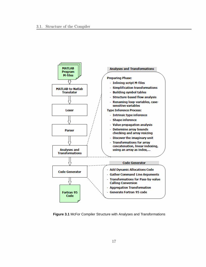
them. McFor is constructed in a conventional way with a series of different phases, as
shown in Figure 3.1. The contributions of this thesis are predominately in the “Anal-
yses and Transformations” and “Code Generator” phases. This section discusses the
main issues and the overall strategy adopted for each phase of the compiler.
3.1.1 MATLAB-to-Natlab Translator
Because the MATLAB language is used for command scripts and as a programming
language at the same time, the syntax of MATLAB is quite convoluted. Since in
command script syntax, the character space is always used as a delimiter, MATLAB
syntax is thus sensitive to spaces; however, in programming language syntax, spaces
are ignored in most cases. As a result, some MATLAB language features cannot
be handled by normal lexing and parsing techniques. Therefore, the McLab team
defined a functionally equivalent subset of MATLAB, called Natlab, which eliminates
most ambiguous MATLAB syntax. The MATLAB-to-Natlab translator is designed
for translating MATLAB programs from MATLAB syntax to Natlab syntax.
3.1.2 Lexer and Parser
The Natlab lexer is specified by using MetaLexer [Cas09], an extensible modular lex-
ical specification language developed by Andrew Casey of McLab team. The Natlab
parser is generated by using JastAdd [EH07], an extensible attribute grammar frame-
work developed by Ekman et al.. McFor uses the same lexer and parser to obtain the
abstract syntax tree (AST) of the input program, then extends the AST with type
inference functions and performs type inference and transformations on it.
1http://www.sable.mcgill.ca/mclab2http://www.sable.mcgill.ca
16
3.1. Structure of the Compiler
Figure 3.1 McFor Compiler Structure with Analyses and Transformations
17
Overview of the McFor Compiler
3.1.3 Analyses and Transformations
The compiler performs type inference and transformations in this phase. It consists
of two sub-phases: the preparation phase (described in Section 3.2) and the type
inference process (described in Section 4.2).
In the preparation phase, the compiler first inlines the script M-files, then performs
the simplification transformation for breaking down complex expressions to reduce
the complexity of type inference. The compiler then performs structure-based flow
analysis to build symbol tables and create type conflict functions, which are used
for explicitly capturing potential type changes. While building the symbol tables,
the compiler renames variables that are treated as different variables in case-sensitive
MATLAB but as the same variable in case-insensitive Fortran.
The second phase is the type inference process, which is an iterative process that
infers types of all variables until reaching a fixed point, where variables’ types will
not be changed any more. It is an interprocedural type inference: when reaching a
function call, the compiler analyzes the called user-defined function, infers the types
in the callee function, and returns back with the inference result. The compiler builds
a database to store inference results for all inferred user-defined functions along with
their function type signatures extracted from calling contexts. The compiler also
transforms codes with special MATLAB features into their functional equivalent forms
to ease the effort of code generation.
3.1.4 Code Generator
In this final phase, the compiler traverses the AST in lexicographic order, and gener-
ates Fortran code using the type information stored in the symbol table.
After a set of transformations, most of MATLAB code can be straightforwardly
translated into Fortran code. In addition, the Code Generator generates extra variable
declarations directly from the declaration nodes created during the type inference
process. It also generates extra statements to gather command line arguments passing
into the program. For user-defined functions, each of them will be translated into a
Fortran subroutine, which is able to return multiple values as MATLAB function does.
18
3.2. Preparation Phase
Each Fortran subroutine has the same list of parameters as the original user-defined
function.
Because MATLAB uses pass-by-value calling conversion and Fortran uses pass-
by-reference conversion, the user-defined functions need special treatments. For each
parameter that appears in the LHS of any assignments inside the function, the Code
Generator creates an extra local variable to substitute the parameter, and adds an as-
signment statement to copy the value from the new parameter to the original variable.
Therefore, the original parameter becomes a local variable, thus any modifications on
this local copy will not be visible to the caller.
For dynamically-allocated array variables, the compiler also needs to add alloca-
tion and deallocation statements in the proper places. Allocatable arrays are those
variables that need to be dynamically allocated at runtime. In the Fortran code,
the function or subroutine that first uses an allocatable array variable will declare the
variable and deallocate it at the end of the function or subroutine. Every user-defined
subroutine that use an allocatable parameter can allocate or reallocate the variable
freely, but never deallocated it.
The Code Generator is also in charge of choosing proper Fortran implementations
for high-level operators based on the types of the operands. For example, the For-
tran built-in routine MATMUL() employs the conventional O(N3) method of matrix
multiplication, so it performs poorly for larger size matrices. Therefore, the Code
Generator will translate the MATLAB matrix multiplication operator into MAT-
MUL() routine only when the operands’ sizes are smaller than 200-by-200; otherwise,
it will translate the multiplication operator into dgemm() routine of BLAS library,
which has been optimized for computing large size matrices.
3.2 Preparation Phase
MATLAB has relatively simple syntax, higher-level operators and functions, and no
variable declarations; those features make MATLAB very easy to program. But be-
hind the simple syntax is much complex semantics that relies on the actual types
of the operands and variables. In order to reduce the complexity of type inference
19
Overview of the McFor Compiler
and preserve the special behaviors of some MATLAB features, the McFor compiler
goes through a preparation phase before starting the actual type inference. The
preparation phase includes the following parts: inlining script M-files, simplification,
renaming loop variables, building the symbol tables and renaming duplicated vari-
ables.
3.2.1 Inlining Script M-files
A MATLAB program consists of a list of files, called M-files, which include sequences
of MATLAB commands and statements. There are two types of M-files: script and
function M-files. A function M-file is a user-defined function that accepts input
arguments and returns result values. It has a function declaration that defines the
input and output parameters, and variables used inside the function are local to this
function (e.g., Table 3.1 (b)). A script M-file (e.g., Table 3.1 (a)) does not have
function declaration; it does not accept input arguments nor returns results. Calling
a script is just like calling a function where the script filename is used as the function
name. In contrast to the function M-files, variables used inside a script M-file are
associated with the scope of the caller. Table 3.1 shows the difference between them.
Table 3.1(a) shows a script M-file for computing the mean of each row of a two
dimensional matrix A. After executing the script, variables in this script, m, n, i,
and R, will be added into the caller’s scope. Table 3.1(b) shows a function M-file
using same code plus a function declaration. In this case, only the value of output
parameter R will be return to the caller, other variables are invisible to the caller.
1 function R=rowmean(A)
2 [m,n] = size(A) [m,n] = size(A)
3 for i=1:m for i=1:m
4 R(i) = sum(A(i,:))/n R(i) = sum(A(i,:))/n
5 end end
(a) script (b) function
Table 3.1 Computing mean of a matrix by script and function
20
3.2. Preparation Phase
Functions and scripts are just two different ways of packaging MATLAB code.
They are used equally in MATLAB; they can call each other at any time. MATLAB
uses the same syntax for calling functions and script M-files.
A MATLAB program can consist of both script and function M-files. In order to
preserve the script M-files behavior, our McFor compiler handles the script M-files
using the following two rules:
1. If a script is the main entry of the program, then it will be converted into
a function, where the filename is the function name and it has no input and
output parameters.
2. If a script is called by other script or function, then this script will be inlined
into the caller.
The McFor compiler inlines script M-files by traversing the AST of the whole-
program. Because a script does not take any arguments nor return values, the state-
ment of calling a user-defined script “foo.m” will be a standalone expression statement
either in command syntax form: foo, or in function syntax form: foo(). Because ex-
pression statements are represented by a unique type node in the AST, script calls can
thus be discovered while traversing the AST. During the traversal, when the compiler
discovers a statement that is calling a user-defined script, it inlines that script M-file
into the caller by replacing the calling statement node with a copy of that script’s
AST. The compiler then recursively traverses into that new merged AST to discover
further script calls.
3.2.2 Distinguishing Function Calls from Variables
Because MATLAB has two syntax forms for calling functions: command and function
syntax form, an identifier in a MATLAB program may represent a variable, or a call
to a function or a script in command syntax depending on the program context. The
calls to user-defined scripts have been handled during the inlining phase (described
in Section 3.2.1). For those command syntax function calls that are associated with
21
Overview of the McFor Compiler
arguments, the MATLAB-to-Natlab translator (described in Section 3.1.1) has con-
verted them into function syntax. The remaining cases are function calls that have no
input arguments. For example, a user-defined function M-file “foo.m” has function
declaration: “function y=foo()”, then its command syntax function call, foo, looks
just like a variable, and may appear in following situations:
1. As a standalone statement: foo
2. In the right-hand side (RHS) of an assignment statement: x=foo
3. Used as an index of array variable A: A(foo, n)
4. Used as an argument of another function call: Bar(foo, n)
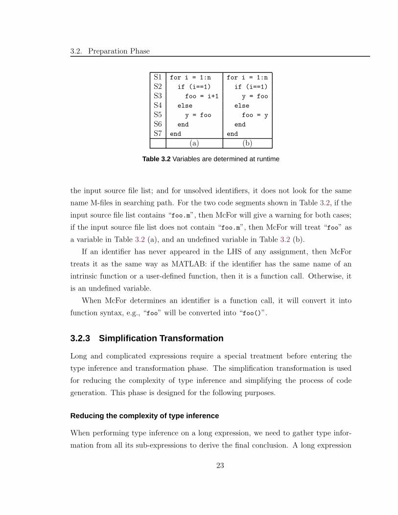
In MATLAB, whether an identifier represents a variable or a function call is
decided at execution time. If an identifier first appears as the left-hand side (LHS) of
an assignment statement, then it is a variable in the whole execution. For example, in
the code segment shown in Table 3.2 (a), since statement S3 will be executed before
S5 at runtime, the identifier “foo” will be treated as a variable. Otherwise if there
exists an intrinsic function with the same name as the identifier, or an M-file with the
same name in the searching path, then it is a function call; if no such function exists,
then it is an undefined variable and will cause a runtime error. When a function
call identifier later appears as a LHS of an assignment statement, then the identifier
becomes a variable, and will stay variable in the rest of execution. For example, if
we change the S3 and S5 as shown in Table 3.2(b), then identifier “foo” is a function
call in S3, and changed to a variable in S5 in the second iteration.
McFor is a batch compiler, it does not have any runtime information about the
program’s execution order; therefore it does not support an identifier having two
meanings in one program. The McFor’s approach is: when an identifier ever appears
as LHS of an assignment statement in the program, then the identifier is a variable.
If a variable in the program has the same name as a user-defined function attached
in the source file list, then McFor will raise a warning, asking user to clarify the use
of that identifier. McFor assumes all user-defined functions and scripts are listed in
22
3.2. Preparation Phase
S1 for i = 1:n for i = 1:n
S2 if (i==1) if (i==1)
S3 foo = i+1 y = foo
S4 else else
S5 y = foo foo = y
S6 end end
S7 end end
(a) (b)
Table 3.2 Variables are determined at runtime
the input source file list; and for unsolved identifiers, it does not look for the same
name M-files in searching path. For the two code segments shown in Table 3.2, if the
input source file list contains “foo.m”, then McFor will give a warning for both cases;
if the input source file list does not contain “foo.m”, then McFor will treat “foo” as
a variable in Table 3.2 (a), and an undefined variable in Table 3.2 (b).
If an identifier has never appeared in the LHS of any assignment, then McFor
treats it as the same way as MATLAB: if the identifier has the same name of an
intrinsic function or a user-defined function, then it is a function call. Otherwise, it
is an undefined variable.
When McFor determines an identifier is a function call, it will convert it into
function syntax, e.g., “foo” will be converted into “foo()”.
3.2.3 Simplification Transformation
Long and complicated expressions require a special treatment before entering the
type inference and transformation phase. The simplification transformation is used
for reducing the complexity of type inference and simplifying the process of code
generation. This phase is designed for the following purposes.
Reducing the complexity of type inference
When performing type inference on a long expression, we need to gather type infor-
mation from all its sub-expressions to derive the final conclusion. A long expression
23
Overview of the McFor Compiler
with complicated structure generates more uncertain elements during the inference
process than simple expressions, thus increases the complexity of making the final
conclusion. By creating temporary variables to represent sub-expressions, we can
use those variables and their symbol table entries to store the type information ac-
quired from those sub-expressions. Therefore, the type inference is split into several
relatively short and simple inference steps with limited complexity.
The need for further transformations
When translating a MATLAB program into Fortran, all the user-defined functions
will be converted into Fortran subroutines, and some MATLAB built-in functions
will also be translated into corresponding Fortran intrinsic subroutines. Because
Fortran subroutine calls do not return any values, thus they cannot be used as ex-
pressions, like its original MATLAB functions calls, by any other expressions. When
a MATLAB function call is used by another expression, this transformation requires
temporary variables to retrieve values from the Fortran subroutine, then put them
back into where they were used. Because those transformations create new temporary
variables, they must be performed before the symbol table is generated. Therefore,
during this simplification phase, we take out function call sub-expressions from long
expressions and transform them into standalone assignment statements. As a result,
the code generator can simply translate the assignment statement into subroutine call
straightforwardly.
Because MATLAB uses the same syntax for function call and array access, and the
simplification process can only recognize sub-expressions based on their structures,
thus this process creates unneeded temporary variables and assignments for array
access sub-expressions. For solving this problem, we design an aggregation phase
(described in Section 5.5) to reverse unnecessary simplifications.
Simplify transformations for linear indexing
MATLAB supports linear indexing, where any element of a matrix can be referred
with a single subscript. This property is widely used in MATLAB programs, espe-
24
3.2. Preparation Phase
cially for row vectors and column vectors, even if they are internally two dimensional
matrices, but indexing by one subscript is very convenient and understandable. How-
ever, in Fortran, each reference to an element of a matrix must specify the indices for
all its dimensions. Therefore, a certain amount of transformations on matrix indexing
must be done when we are compiling MATLAB programs. To simplify those trans-
formations, we create temporary variables, take out matrix access sub-expressions
from long expressions and insert them into standalone assignment statements before
applying the type inference and transformations.
The compiler creates a new temporary variable uniquely for every sub-expression
extracted from a long expression, and inserts the new assignment statement for the
temporary variable immediately above the statement that contains the long expres-
sion. Therefore, the new assignment statements do not change the flow dependence
of the program.
This simplification process is a recursive process on each node of the AST. After
traversing the AST once, all simplifications will have been completed.
Table 3.3 shows an example of the simplification transformation. Table 3.3 (a)
shows a MATLAB assignment statement which has a complicated right hand side
expression. Table 3.3 (b) shows the code in MATLAB syntax after a sequence of
simplification transformations. Variable tmp 4 is created for the function call sub-
expression inside the original RHS expression. Variable tmp 3 is created for simplifying
the argument of the function call. Variable tmp 1 and tmp 2 are created for the
two sub-expressions of that argument respectively. Another transformation has been
performed on variable tmp 2 at statement S2 where tmp 2 represents a column vector
and its RHS is a one dimensional array.
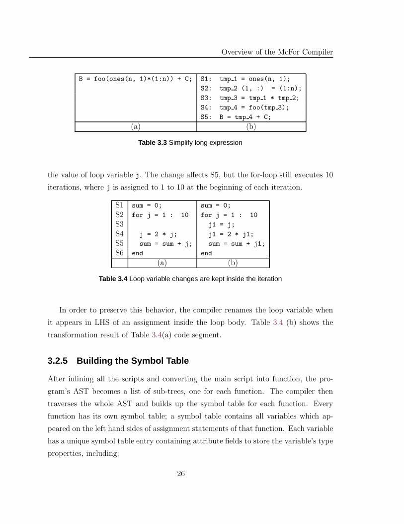
3.2.4 Renaming Loop-Variables
In MATLAB, a loop variable can be assigned to different values inside the loop but
the changes only affect current iteration. When the next iteration starts, the loop
variable will be assigned to the correct value as it has never been changed.
For example, in the code fragment shown in Table 3.4(a), statement S4 changes
25
Overview of the McFor Compiler
B = foo(ones(n, 1)*(1:n)) + C; S1: tmp 1 = ones(n, 1);
S2: tmp 2 (1, :) = (1:n);
S3: tmp 3 = tmp 1 * tmp 2;
S4: tmp 4 = foo(tmp 3);
S5: B = tmp 4 + C;
(a) (b)
Table 3.3 Simplify long expression
the value of loop variable j. The change affects S5, but the for-loop still executes 10
iterations, where j is assigned to 1 to 10 at the beginning of each iteration.
S1 sum = 0; sum = 0;
S2 for j = 1 : 10 for j = 1 : 10
S3 j1 = j;
S4 j = 2 * j; j1 = 2 * j1;
S5 sum = sum + j; sum = sum + j1;
S6 end end
(a) (b)
Table 3.4 Loop variable changes are kept inside the iteration
In order to preserve this behavior, the compiler renames the loop variable when
it appears in LHS of an assignment inside the loop body. Table 3.4 (b) shows the
transformation result of Table 3.4(a) code segment.
3.2.5 Building the Symbol Table
After inlining all the scripts and converting the main script into function, the pro-
gram’s AST becomes a list of sub-trees, one for each function. The compiler then
traverses the whole AST and builds up the symbol table for each function. Every
function has its own symbol table; a symbol table contains all variables which ap-
peared on the left hand sides of assignment statements of that function. Each variable
has a unique symbol table entry containing attribute fields to store the variable’s type
properties, including:
26
3.2. Preparation Phase
• Intrinsic type, which could be logical, integer, real, double precision or complex;
• Shape, which includes the number of dimensions and size of each dimension. A
scalar variable has zero dimensions.
• Value range, which includes the minimum and maximum estimated values.
Because the MATLAB language is case-sensitive for variable names but Fortran
is not, variables composed by same sequence of characters but in different cases are
different variables in MATLAB but are treated as one variable in Fortran. In order
to solve this problem, a variable, before being added into the symbol table, is checked
to see if its case-insensitive version creates a duplicate. If a duplication is discovered,
then the compiler renames the variable in the whole program and adds the renamed
variable into the symbol table.
27

Overview of the McFor Compiler
28
Chapter 4
Type Inference Mechanism
Type inference is the core of the McFor compiler. In this chapter, we present our
type inference mechanism. The type inference principles are described in Section 4.1,
followed by the type inference process (Section 4.2), the intermediate representation
and type conflict functions (Section 4.3). How to solve the type changes between
multiple assignments and type conflict functions is discussed in Section 4.4 and 4.5.
For shape inference, the value propagation analysis is discuss in Section 4.6, and how
to determine variable shape at runtime is discussed in Section 4.7. In Section 4.8, we
describe some additional analyses that are required during the type inference process.
4.1 Type Inference Principles
A variable’s type consists of three parts of information, intrinsic type, shape, and
value range. In this section, we explain the principle of intrinsic type inference, and
the shape inference.
4.1.1 Intrinsic Type Inference
Our approach of determining variables’ intrinsic types follows a mathematical frame-
work based on the theory of lattices proposed by Kaplan and Ullman [KU80]. Pramod
29
Type Inference Mechanism
and Prithviraj also used this framework in their MATLAB type inference engine
MAGICA [JB01, JB02].
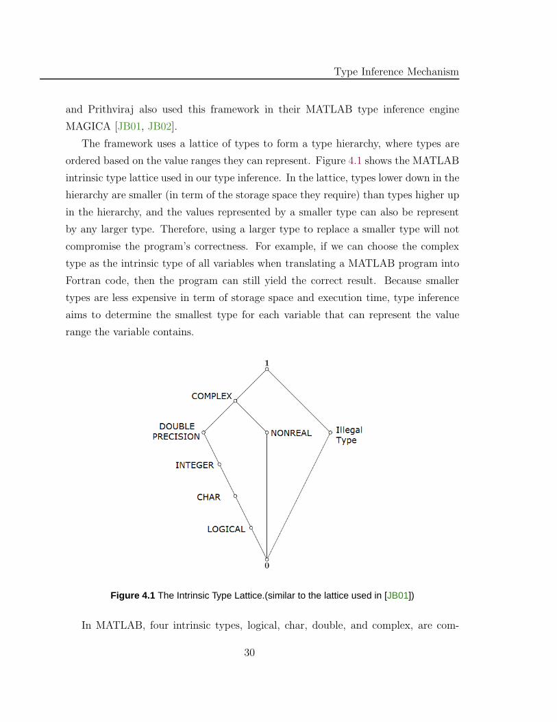
The framework uses a lattice of types to form a type hierarchy, where types are
ordered based on the value ranges they can represent. Figure 4.1 shows the MATLAB
intrinsic type lattice used in our type inference. In the lattice, types lower down in the
hierarchy are smaller (in term of the storage space they require) than types higher up
in the hierarchy, and the values represented by a smaller type can also be represent
by any larger type. Therefore, using a larger type to replace a smaller type will not
compromise the program’s correctness. For example, if we can choose the complex
type as the intrinsic type of all variables when translating a MATLAB program into
Fortran code, then the program can still yield the correct result. Because smaller
types are less expensive in term of storage space and execution time, type inference
aims to determine the smallest type for each variable that can represent the value
range the variable contains.
Figure 4.1 The Intrinsic Type Lattice.(similar to the lattice used in [JB01])
In MATLAB, four intrinsic types, logical, char, double, and complex, are com-
30
4.1. Type Inference Principles
monly used in mathematic computations. When translating to Fortran code, a vari-
able will have one of the five Fortran intrinsic types: logical, character, integer, double
precision, and complex. As the lattice shown in Figure 4.1, the complex type is at
the top of the hierarchy, followed by double precision, integer, char, and the logical
type is at the bottom.
Our type inference approach aims to infer the smallest type for a variable that can
represent the value it contains. For example, if we estimate a variable only contains
integer values throughout the whole program, then we will decide the variable has an
integer type. When a variable is assigned to a value with a type different from its
current type, then we will merge those two types based on the type hierarchy, and
use the larger type to be the final type. (The details of the type merging process are
described in the following sections.) This approach can reduce the need for creating
new variables to hold the new type during the type changes.
4.1.2 Sources of Type Inference
The type inference extracts type information from four sources: program constants,
operators, built-in functions, and function calling contexts.
Constants
Program constants provide precise information about intrinsic type, shape, and value;
they provide the starting point of our type inference. For example, constant 10.5 is
a double scalar with the value 10.5.
Operators
MATLAB has three kinds of operators: arithmetic, relational, and logical operators.
Relational and logical operators always return the results of the logical type. But
MATLAB arithmetic operators are highly overloaded; they can accept different types
of operands and yield different types of results. Therefore, we need create a set of
type functions for each operator on different type operands. For example, Table 4.1
shows the result types of type functions of operator “+” for different types of operands.
31
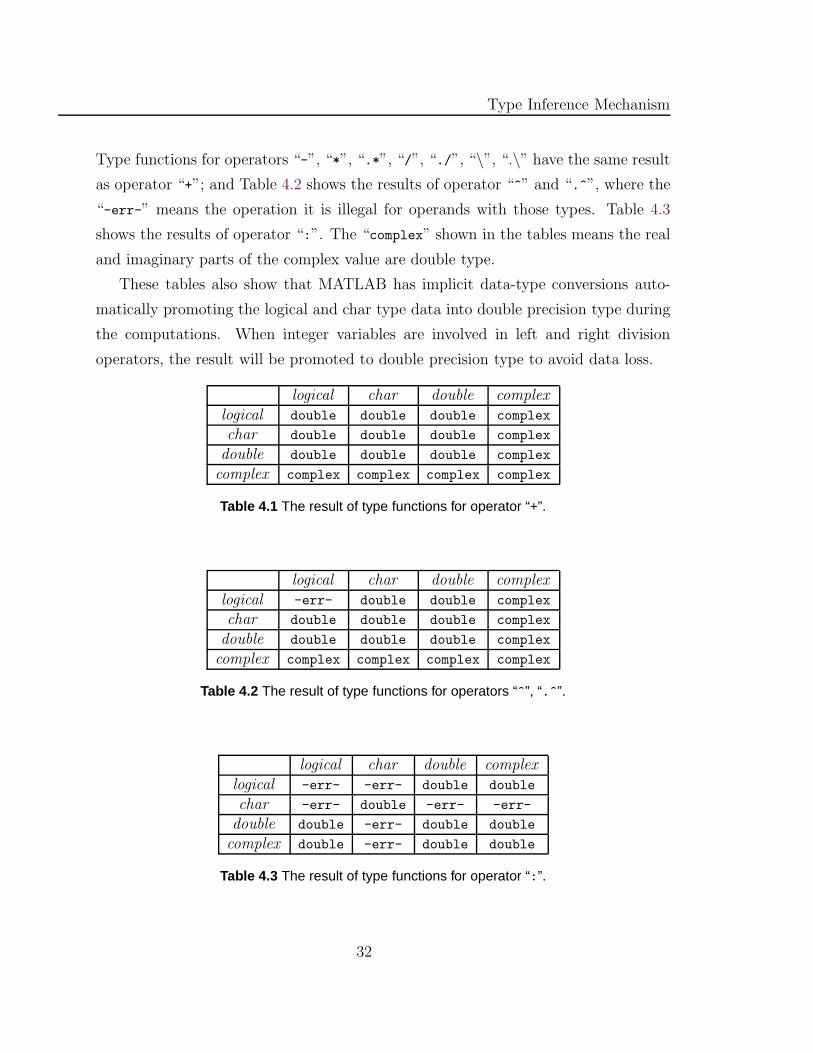
Type Inference Mechanism
Type functions for operators “-”, “*”, “.*”, “/”, “./”, “\”, “.\” have the same result
as operator “+”; and Table 4.2 shows the results of operator “^” and “.^”, where the
“-err-” means the operation it is illegal for operands with those types. Table 4.3
shows the results of operator “:”. The “complex” shown in the tables means the real
and imaginary parts of the complex value are double type.
These tables also show that MATLAB has implicit data-type conversions auto-
matically promoting the logical and char type data into double precision type during
the computations. When integer variables are involved in left and right division
operators, the result will be promoted to double precision type to avoid data loss.
logical char double complexlogical double double double complex
char double double double complex
double double double double complex
complex complex complex complex complex
Table 4.1 The result of type functions for operator “+”.
logical char double complexlogical -err- double double complex
char double double double complex
double double double double complex
complex complex complex complex complex
Table 4.2 The result of type functions for operators “^”, “.^”.
logical char double complexlogical -err- -err- double double
char -err- double -err- -err-
double double -err- double double
complex double -err- double double
Table 4.3 The result of type functions for operator “:”.
32
4.1. Type Inference Principles
MATLAB operators not only define the shape and size information for the result
data, but provide constraints on the type and shape of operand variables. MATLAB
operators have conformability requirements for matrix operands. For example, when
two operands are matrices, operators “*”, “-”, and logical operators require the
operands must have the same shape, and result value will have the same shape as
well. For another group of operators “*”, “\”, and “/”, if two operands are matrices,
then they must be two-dimensional and the sizes of their inner dimensions must equal.
For example, for statement B*C, if variable B has shape of n-by-m, and C has shape of
p-by-q, then m must equal to p and the result will have the shape of n-by-q.
One example of using this kind of constraints is to determine vectors in linear
indexing, like the expression ones(n,1)*(1:n) shown in Table 3.3 (a). The simplifi-
cation phase generates temporary variable tmp 2 to represent the expression (1:n),
which is a one-dimensional array. According to the conformability requirements of
matrix multiplication, tmp 2 must be a two-dimensional matrix where the size of the
first dimension is 1. Therefore, we change the shape of tmp 2 and adjust the subscripts
of tmp 2 in statement S2 into tmp 2(1,:)=(1:n).
Built-in Functions
MATLAB’s built-in functions are also highly overloaded; they accept a varying num-
ber of arguments with different types. But since the built-in functions are well defined
by MATLAB, they can provide precise type information of return results for each com-
bination of input parameters. Thus, the McFor compiler built up a database for the
type inference process that contains all type signatures (described in 4.2.1) of each
built-in function and their corresponding return types.
Calling Context
From each calling context, the compiler gathers the types of all arguments to form
a function type signature (described in 4.2.1), and then uses it to determine which
version of translated code should be executed. When there is no matched version of
code, the compiler then uses those input parameter types to perform type inference
33
Type Inference Mechanism
on the user-defined function.
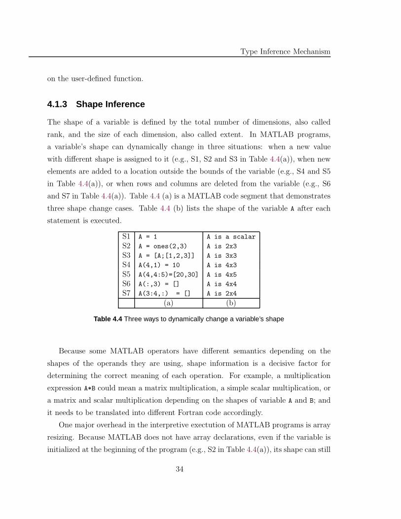
4.1.3 Shape Inference
The shape of a variable is defined by the total number of dimensions, also called
rank, and the size of each dimension, also called extent. In MATLAB programs,
a variable’s shape can dynamically change in three situations: when a new value
with different shape is assigned to it (e.g., S1, S2 and S3 in Table 4.4(a)), when new
elements are added to a location outside the bounds of the variable (e.g., S4 and S5
in Table 4.4(a)), or when rows and columns are deleted from the variable (e.g., S6
and S7 in Table 4.4(a)). Table 4.4 (a) is a MATLAB code segment that demonstrates
three shape change cases. Table 4.4 (b) lists the shape of the variable A after each
statement is executed.
S1 A = 1 A is a scalar
S2 A = ones(2,3) A is 2x3
S3 A = [A;[1,2,3]] A is 3x3
S4 A(4,1) = 10 A is 4x3
S5 A(4,4:5)=[20,30] A is 4x5
S6 A(:,3) = [] A is 4x4
S7 A(3:4,:) = [] A is 2x4
(a) (b)
Table 4.4 Three ways to dynamically change a variable’s shape
Because some MATLAB operators have different semantics depending on the
shapes of the operands they are using, shape information is a decisive factor for
determining the correct meaning of each operation. For example, a multiplication
expression A*B could mean a matrix multiplication, a simple scalar multiplication, or
a matrix and scalar multiplication depending on the shapes of variable A and B; and
it needs to be translated into different Fortran code accordingly.
One major overhead in the interpretive exectution of MATLAB programs is array
resizing. Because MATLAB does not have array declarations, even if the variable is
initialized at the beginning of the program (e.g., S2 in Table 4.4(a)), its shape can still
34
4.2. Type Inference Process
be changed when the indexed array access is outside the array bounds (e.g., S4 and S5
in Table 4.4(a)). Therefore, a major goal of our shape inference on array variables is
to determine the largest number of dimensions and the largest size of each dimension
that are used on those variables in the program. By using those information, we
can declare the array variables statically or dynamically allocate them once in the
Fortran code; thus the overhead of array dynamically resizing, moving data around,
and checking array bounds can be avoided.
4.2 Type Inference Process
The McFor compiler performs whole-program analysis on the input MATLAB pro-
gram. Because a MATLAB program usually contains several user-defined functions,
interprocedural analysis is necessary for determining the type information of a func-
tion’s output parameters according to each calling context.
4.2.1 Function Type Signature
For a user-defined function with n input parameters, the list of those parameters’
types along with the function name forms the type signature of this function, e.g,
foo{T1, T2, . . . , Tn}. Because of the dynamically-typed nature of MATLAB, function
declarations do not define the types of input parameters, thus a function can be
called by using different types of arguments. Different types of input parameters may
cause different type inference and transformation results on the function, thus we
need create separate copies of the function AST for different calling contexts. We use
function type signatures to determine which version of the function code should be
used for a giving calling context. The McFor compiler uses a database to store all
the function type signatures, along with their corresponding AST root node pointers
and list of output parameters’ types.
35
Type Inference Mechanism
4.2.2 Whole-Program Type Inference
The type inference process starts from the main function’s AST1, traverses every node
of the main function from top to bottom. When encountering a call to a user-defined
function, the compiler first gathers the type information of each argument to form a
function type signature, then compares it with function type signatures stored in the
database. If there is a matched function type signature, the compiler then uses the
corresponding inference result, the list of its output parameters’ types, and continues
the type inference process. If there is no matched type signature, then the compiler
will make a copy of the calling function’s AST, and perform type inference on it with
the new calling context. After finishing type inference on the calling function and
collecting its output parameters’ types, the compiler stores the function type signature
and the inference result into database, then returns to the location where the function
call happened, and continues on the remaining nodes. For nested function calls, the
compiler performs type inference on those functions recursively to generate inference
results for each call.
If a user-defined function is a recursive function, the compiler uses the following
strategy. Because a recursive function must have a code segment that implements
the base case of its recursive algorithm and includes assignments for all its return
variables, the compiler can obtain the types of all return variables from there. There-
fore, in the first inference iteration, the compile ignores recursive function calls and
uses those types inferred from base case code segment as the temporary result. In
the following inference iterations, the compiler will use this temporary result to infer
the final result.
The type inference is performed with structure-based flow analysis on the AST of
the program. For each function, the type inference process is an iterative process that
infers the types of all variables until reaching a fixed point, where variables’ types
will not be changed any more.
1The compiler assumes the first file in the input source file list is the main function of the program
36
4.2. Type Inference Process
4.2.3 The Type Inference Algorithm
In the type inference process, the compiler goes through the program in lexicographic
order, analyzes each assignment statement, and takes following actions according to
the type of statement.
• For an assignment statement whose RHS is a constant:
– Return the intrinsic type and shape of the constant. e.g., 2.5 is a double
scalar, [10, 5] is a one-dimensional integer array of size 2.
• For an assignment statement whose RHS is a variable:
– If the variable is an array with subscripts, First determine the shape it
represents (either a partial array or an element), then return the shape
with the intrinsic type of the variable stored in the symbol table. For
example, if A is integer array of size m-by-n, then A(1,:) is one-dimension
integer array of size n.
– Otherwise, return the intrinsic type and shape of that variable stored in
the symbol table.
• For an assignment statement whose RHS is a computational expression,
– Based on the operands’ intrinsic types and shapes, recursively calculate
the intrinsic type and shape of the expression according to operator result
tables (Table 4.1, 4.2, and 4.3), then return the result.
• For an assignment statement whose RHS is a built-in function:
– Return the result type according to built-in function database. For exam-
ple, randn(m,n) returns a two-dimensional matrix of size m-by-n.
• For an assignment statement whose RHS is a user-defined function:
– Form the function type signature from the calling context, and check it in
the database,
37
Type Inference Mechanism
∗ If there is a match, return the stored result types
∗ Otherwise,
· If it is a recursive call, then ignore this statement.
· Otherwise, perform type inference on the function, return the in-
ference result.
• For an assignment statement whose RHS is alpha-function:
– Perform analysis described in Section 4.5.1
• For an assignment statement whose RHS is beta-function:
– Perform analysis described in Section 4.5.2
• For an assignment statement whose RHS is lambda-function:
– Perform analysis described in Section 4.5.3
• Other non-assignment statement
– If it is a user-defined function call, check the database
∗ if there is a matched type signature, ignore
∗ otherwise, perform type inference on the function
– Otherwise, ignore.
4.3 Intermediate Representation and Type Conflict Func-
tions
The goal of type inference is to determine each variable’s type properties: intrinsic
type, shape, and value range, which will be used by the compiler to generate the
Fortran declarations and to perform optimizations.
MATLAB is a dynamically-typed language; variables can change their types at
runtime. However, in Fortran, a variable can only be statically declared as one type.
38
4.3. Intermediate Representation and Type Conflict Functions
Therefore, every time when a variable’s type changes, we need to either treat the
variable as a new variable, or change the variable’s final type.
This section discusses the usefulness of static single-assignment (SSA) representa-
tion in type inference and introduces type conflict functions to capture type changes.
4.3.1 Disadvantages of SSA Form in Type Inference
In the McFor compiler, we did not use a SSA representation because a SSA represen-
tation cares about the values that variables contain, but type inference cares about
the types of those variables.
A program is in SSA form if every variable only appears as the target of one
assignment where a value is assigned to it, which implies for each use of a variable,
there is only one definition. The SSA representation is designed for separating values
from their locations by creating unique variables to represent each value. Thus, SSA
representation is very effective for value-related optimizing transformations, such as
constant propagation and value numbering. However, type inference aims to solve the
type of each variable, where the type of the value is important, not the value itself.
Also, while translating a program to SSA form, the translation process renames a
variable every time a new value is assigned to the variable. When the value has the
same type as the variable’s, the renaming is unnecessary from type inference’s point of
view. In a normal program, a variable’s type changes far less frequently than its value
changes. Therefore, creating new variables for building an unique relation between a
value and a variable does not make type inference efficient; on the contrary, the new
created variables make the program even more unlike the original one, hence reduce
the program’s readability.
Moreover, translating array computation programs into SSA representation usu-
ally needs complex analysis. The SSA representation efficiently handles scalar vari-
ables and some array variables when they are used without subscripts for representing
whole arrays during the assignment (e.g., A=1, means assigning 1 to all element of ar-
ray A). But, when array variables are used with subscripts for representing partial
arrays (e.g., A(1,:)=1, means assigning 1 to every element in the first row of ar-
39
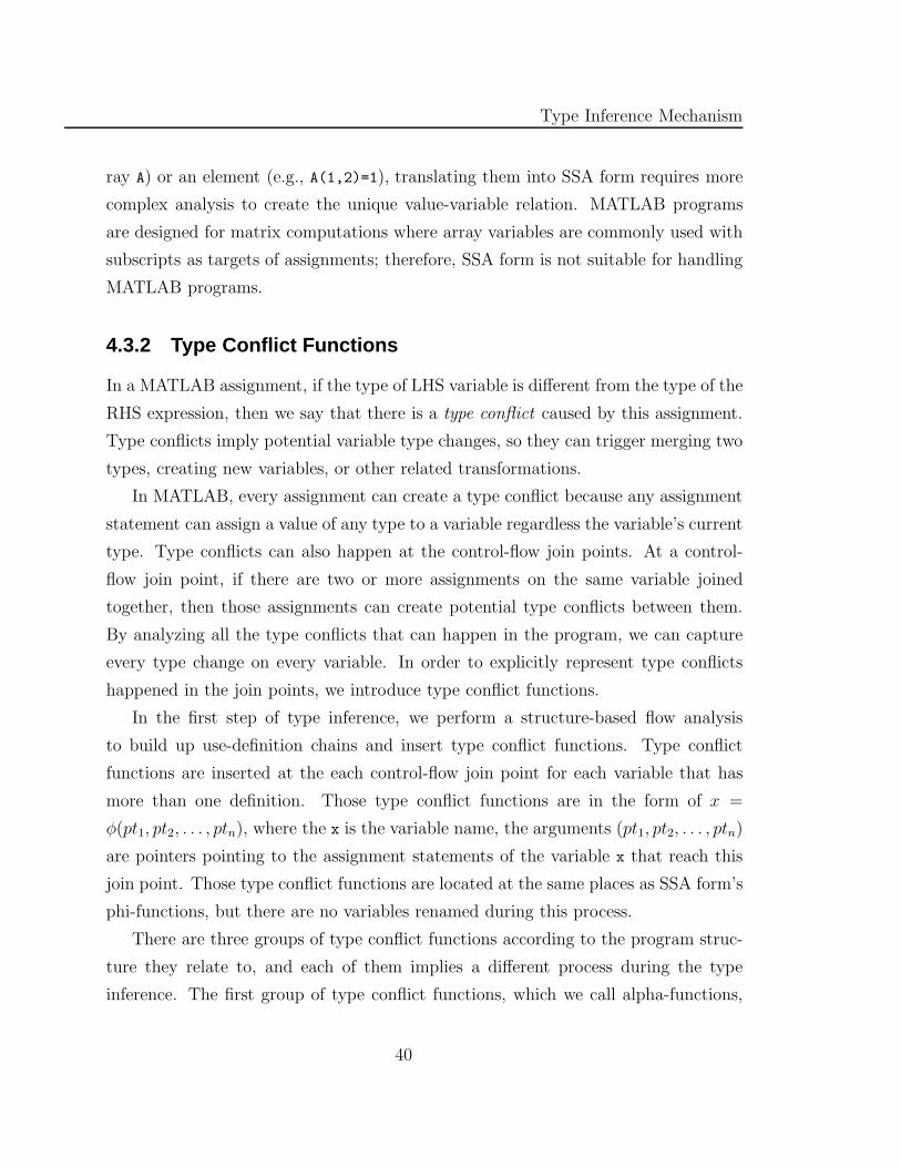
Type Inference Mechanism
ray A) or an element (e.g., A(1,2)=1), translating them into SSA form requires more
complex analysis to create the unique value-variable relation. MATLAB programs
are designed for matrix computations where array variables are commonly used with
subscripts as targets of assignments; therefore, SSA form is not suitable for handling
MATLAB programs.
4.3.2 Type Conflict Functions
In a MATLAB assignment, if the type of LHS variable is different from the type of the
RHS expression, then we say that there is a type conflict caused by this assignment.
Type conflicts imply potential variable type changes, so they can trigger merging two
types, creating new variables, or other related transformations.
In MATLAB, every assignment can create a type conflict because any assignment
statement can assign a value of any type to a variable regardless the variable’s current
type. Type conflicts can also happen at the control-flow join points. At a control-
flow join point, if there are two or more assignments on the same variable joined
together, then those assignments can create potential type conflicts between them.
By analyzing all the type conflicts that can happen in the program, we can capture
every type change on every variable. In order to explicitly represent type conflicts
happened in the join points, we introduce type conflict functions.
In the first step of type inference, we perform a structure-based flow analysis
to build up use-definition chains and insert type conflict functions. Type conflict
functions are inserted at the each control-flow join point for each variable that has
more than one definition. Those type conflict functions are in the form of x =
φ(pt1, pt2, . . . , ptn), where the x is the variable name, the arguments (pt1, pt2, . . . , ptn)
are pointers pointing to the assignment statements of the variable x that reach this
join point. Those type conflict functions are located at the same places as SSA form’s
phi-functions, but there are no variables renamed during this process.
There are three groups of type conflict functions according to the program struc-
ture they relate to, and each of them implies a different process during the type
inference. The first group of type conflict functions, which we call alpha-functions,
40
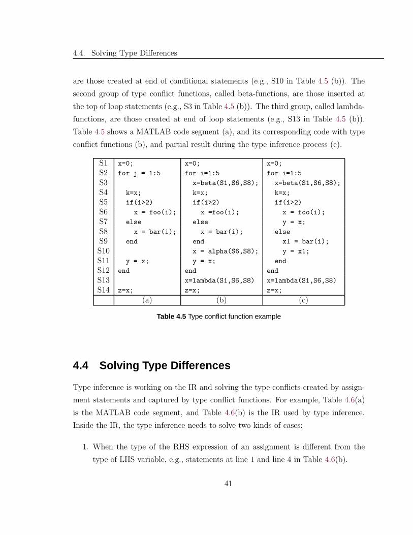
4.4. Solving Type Differences
are those created at end of conditional statements (e.g., S10 in Table 4.5 (b)). The
second group of type conflict functions, called beta-functions, are those inserted at
the top of loop statements (e.g., S3 in Table 4.5 (b)). The third group, called lambda-
functions, are those created at end of loop statements (e.g., S13 in Table 4.5 (b)).
Table 4.5 shows a MATLAB code segment (a), and its corresponding code with type
conflict functions (b), and partial result during the type inference process (c).
S1 x=0; x=0; x=0;
S2 for j = 1:5 for i=1:5 for i=1:5
S3 x=beta(S1,S6,S8); x=beta(S1,S6,S8);
S4 k=x; k=x; k=x;
S5 if(i>2) if(i>2) if(i>2)
S6 x = foo(i); x =foo(i); x = foo(i);
S7 else else y = x;
S8 x = bar(i); x = bar(i); else
S9 end end x1 = bar(i);
S10 x = alpha(S6,S8); y = x1;
S11 y = x; y = x; end
S12 end end end
S13 x=lambda(S1,S6,S8) x=lambda(S1,S6,S8)
S14 z=x; z=x; z=x;
(a) (b) (c)
Table 4.5 Type conflict function example
4.4 Solving Type Differences
Type inference is working on the IR and solving the type conflicts created by assign-
ment statements and captured by type conflict functions. For example, Table 4.6(a)
is the MATLAB code segment, and Table 4.6(b) is the IR used by type inference.
Inside the IR, the type inference needs to solve two kinds of cases:
1. When the type of the RHS expression of an assignment is different from the
type of LHS variable, e.g., statements at line 1 and line 4 in Table 4.6(b).
41
Type Inference Mechanism
2. When a variable’s multiple definitions reach a control-flow join point, which is
represented by a type conflict function, e.g., statements at line 3 and line 6 in
Table 4.6(b).
In either case, the compiler will first solve the difference between intrinsic types,
then solve the difference between shapes.
1stiteration 2nditeration1 sum=0; sum=0; integer double2 for i = 1:10 for i = 1:10
3 sum=beta(S1,S4) double4 sum=sum+i/2; sum=sum+i/2; double double5 end end
6 sum=lambda(S1,S4) double double(a) (b) (c) (d)
Table 4.6 Type inference example.
4.4.1 Merging Intrinsic Types
In the above two cases, the compiler will choose the largest intrinsic type among
them, based on the type hierarchy described in Section 4.1.1, to be the final intrinsic
type of the variable.
Let’s take the process of inferring the type of variable sum in Table 4.6 as an
example. In the first iteration of type inference process, the variable sum becomes
an integer type variable at assignment of line 1. At line 3, the compiler postpones
the inference on the beta function until the end of the loop because it has forward
reference. At line 4, since the RHS expression has the double type, which is larger
than the integer type, the sum thus becomes a double type variable. At the end of
loop, the compiler processes the beta function of line 3 and lambda function of line
6, and chooses the larger type for sum from line 1 and line 4, which is also the double
type. Then the compiler starts the second iteration of the type inference process.
Since the type of sum is still inferred as the double type, the compiler concludes that
sum is a double type variable.
42
4.4. Solving Type Differences
After type inference, some assignment statements may be illegal in Fortran. For
example, in MATLAB, variables of logical or char types can participate in any arith-
metic computations, but they are forbidden in Fortran. Therefore, we designed an
extra transformation phase (described in Chapter 5) to solve those problems after the
type inference process.
4.4.2 Solving Differences Between Shapes
As described in Section 4.1.3, the shape of a variable can be changed in three situa-
tions, when a new value with different shape is assigned to it (e.g., S1, S2 and S3 in
Table 4.4(a)), when new elements are added to an array outside the bounds of the
variable (e.g., S4 and S5 in Table 4.4(a)), or when rows and columns are deleted from
the variable (e.g., S6 and S7 in Table 4.4(a)). Before performing type inference, the
compiler needs to transform the array concatenation case (e.g., S3 in Table 4.4 (a))
to indexed array assignment form, as described below.
Handle Array Concatenations
In MATLAB, one way of expanding an array is to concatenate new elements or blocks
onto the array, where the new elements and blocks are compatible in size with the
original array. Table 4.7 (a) shows an example that uses the array concatenation.
The array variable mag is initialized to zero rows and two columns at statement S1.
In assignment statement S6, mag concatenates with variable newdata, a two column
vector, and the result is assigned back to mag. The array concatenation usually
happens in a loop; in this example, mag will have 10 rows after the execution.
For the statements that are inside a loop, the current inference mechanism uses
the loop variable to carry the number of iterations, and only infers the statements
once. Because the variable mag doesn’t associate with the loop variable i, it is dif-
ficult to be inferred directly by the current inference mechanism. Therefore, for an
array concatenation expression, we applied an extra transformation to convert the
concatenation to another form of expanding array, using array accesses (S6 in Table
4.7 (b)). Table 4.7 (b) shows the transformed code of Table 4.7 (a). By applying
43
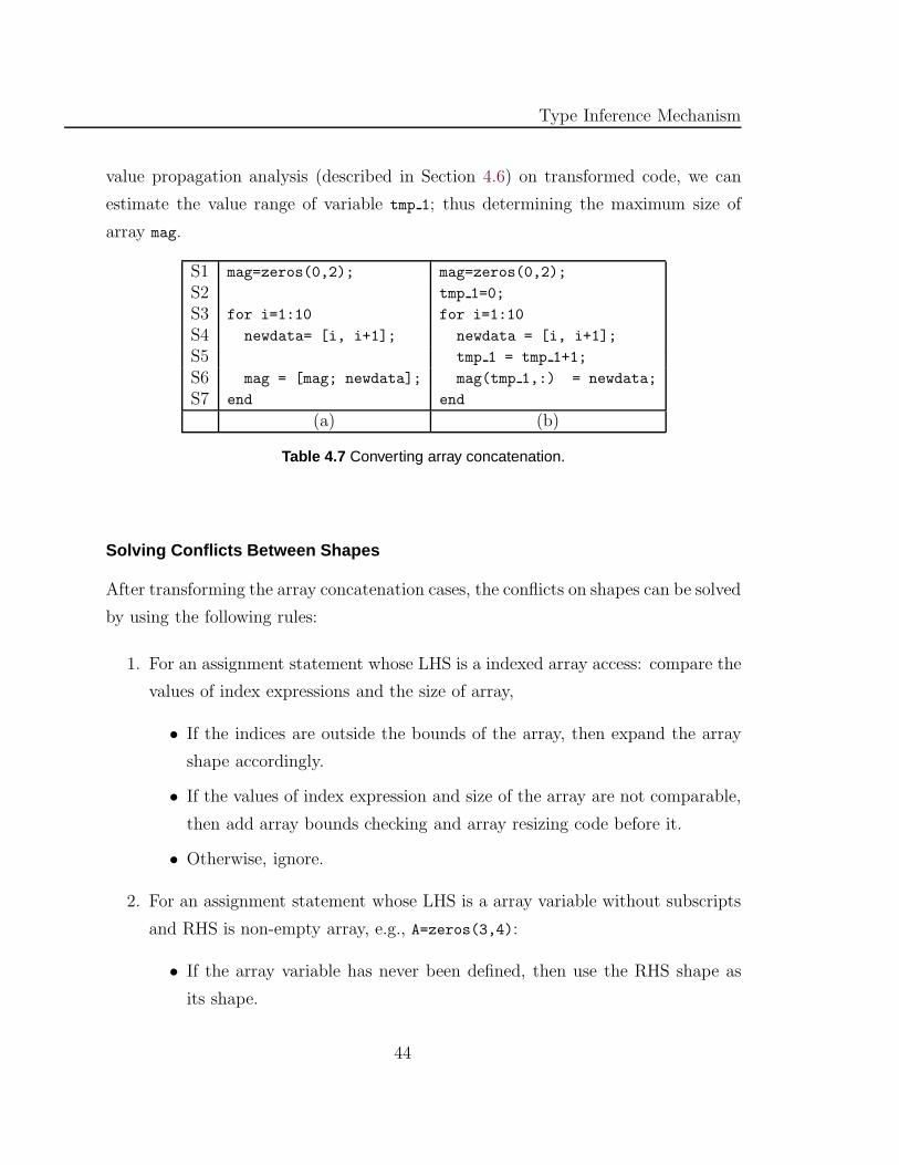
Type Inference Mechanism
value propagation analysis (described in Section 4.6) on transformed code, we can
estimate the value range of variable tmp 1; thus determining the maximum size of
array mag.
S1 mag=zeros(0,2); mag=zeros(0,2);
S2 tmp 1=0;
S3 for i=1:10 for i=1:10
S4 newdata= [i, i+1]; newdata = [i, i+1];
S5 tmp 1 = tmp 1+1;
S6 mag = [mag; newdata]; mag(tmp 1,:) = newdata;
S7 end end
(a) (b)
Table 4.7 Converting array concatenation.
Solving Conflicts Between Shapes
After transforming the array concatenation cases, the conflicts on shapes can be solved
by using the following rules:
1. For an assignment statement whose LHS is a indexed array access: compare the
values of index expressions and the size of array,
• If the indices are outside the bounds of the array, then expand the array
shape accordingly.
• If the values of index expression and size of the array are not comparable,
then add array bounds checking and array resizing code before it.
• Otherwise, ignore.
2. For an assignment statement whose LHS is a array variable without subscripts
and RHS is non-empty array, e.g., A=zeros(3,4):
• If the array variable has never been defined, then use the RHS shape as
its shape.
44
4.5. Type Inference on Type Conflict Functions
• If the RHS shape is different to the LHS shape, then the compiler will
create a new variable and rename the LHS variable and all its appearances
in the rest of program, and add the renamed variable into the symbol table
with the new shape.
• Otherwise, ignore.
3. For an assignment statement whose RHS is empty array:
• Then the compiler will create a new variable, transform the statement into
another assignment that copies all the data from old variable to the new
variable. For example, A(3:4,:)=[] will be transformed into A1=A(1:2,
:). The compiler will then rename the old variable and all its appearances
in the rest of program, and add the renamed variable into the symbol
table with the new shape. The new shape is the variable’s shape minus
the shape represented by LHS array or array access. For example, if array
A is a 4-by-4 matrix, then A1 will be a 2-by-4 matrix.
4. For an assignment statement whose RHS is alpha/beta/lambda functions:
• If there is no renaming happening at all the joined definitions, then use
the largest shape as result shape.
• Otherwise, apply the solution described in Section 4.5.1, 4.5.2, and 4.5.3.
4.5 Type Inference on Type Conflict Functions
During the type inference, when two types cannot be merged together, (which is called
an unsolvable type conflict), a new variable of the new type needs to be created. This
section discusses how the type inference handles unsolvable type conflicts that are
captured by type conflict functions.
45
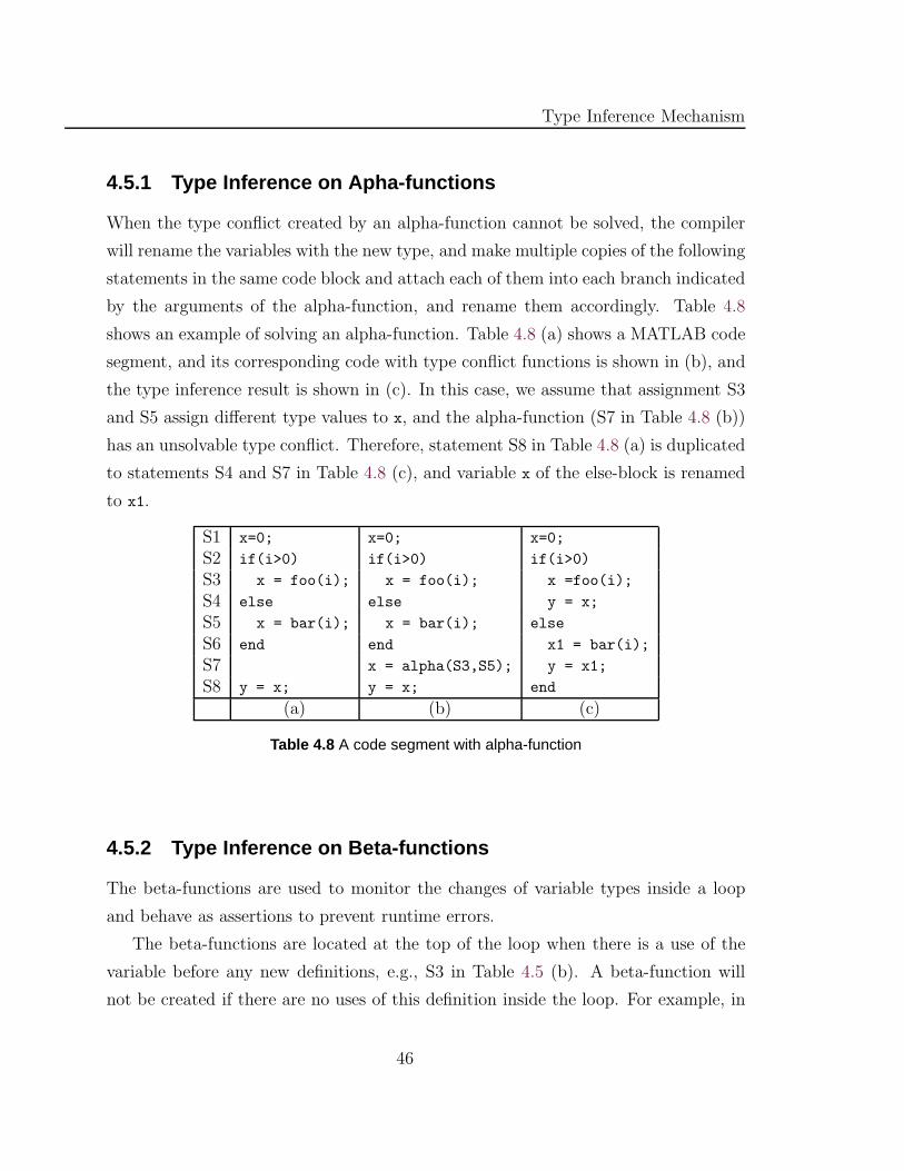
Type Inference Mechanism
4.5.1 Type Inference on Apha-functions
When the type conflict created by an alpha-function cannot be solved, the compiler
will rename the variables with the new type, and make multiple copies of the following
statements in the same code block and attach each of them into each branch indicated
by the arguments of the alpha-function, and rename them accordingly. Table 4.8
shows an example of solving an alpha-function. Table 4.8 (a) shows a MATLAB code
segment, and its corresponding code with type conflict functions is shown in (b), and
the type inference result is shown in (c). In this case, we assume that assignment S3
and S5 assign different type values to x, and the alpha-function (S7 in Table 4.8 (b))
has an unsolvable type conflict. Therefore, statement S8 in Table 4.8 (a) is duplicated
to statements S4 and S7 in Table 4.8 (c), and variable x of the else-block is renamed
to x1.
S1 x=0; x=0; x=0;
S2 if(i>0) if(i>0) if(i>0)
S3 x = foo(i); x = foo(i); x =foo(i);
S4 else else y = x;
S5 x = bar(i); x = bar(i); else
S6 end end x1 = bar(i);
S7 x = alpha(S3,S5); y = x1;
S8 y = x; y = x; end
(a) (b) (c)
Table 4.8 A code segment with alpha-function
4.5.2 Type Inference on Beta-functions
The beta-functions are used to monitor the changes of variable types inside a loop
and behave as assertions to prevent runtime errors.
The beta-functions are located at the top of the loop when there is a use of the
variable before any new definitions, e.g., S3 in Table 4.5 (b). A beta-function will
not be created if there are no uses of this definition inside the loop. For example, in
46
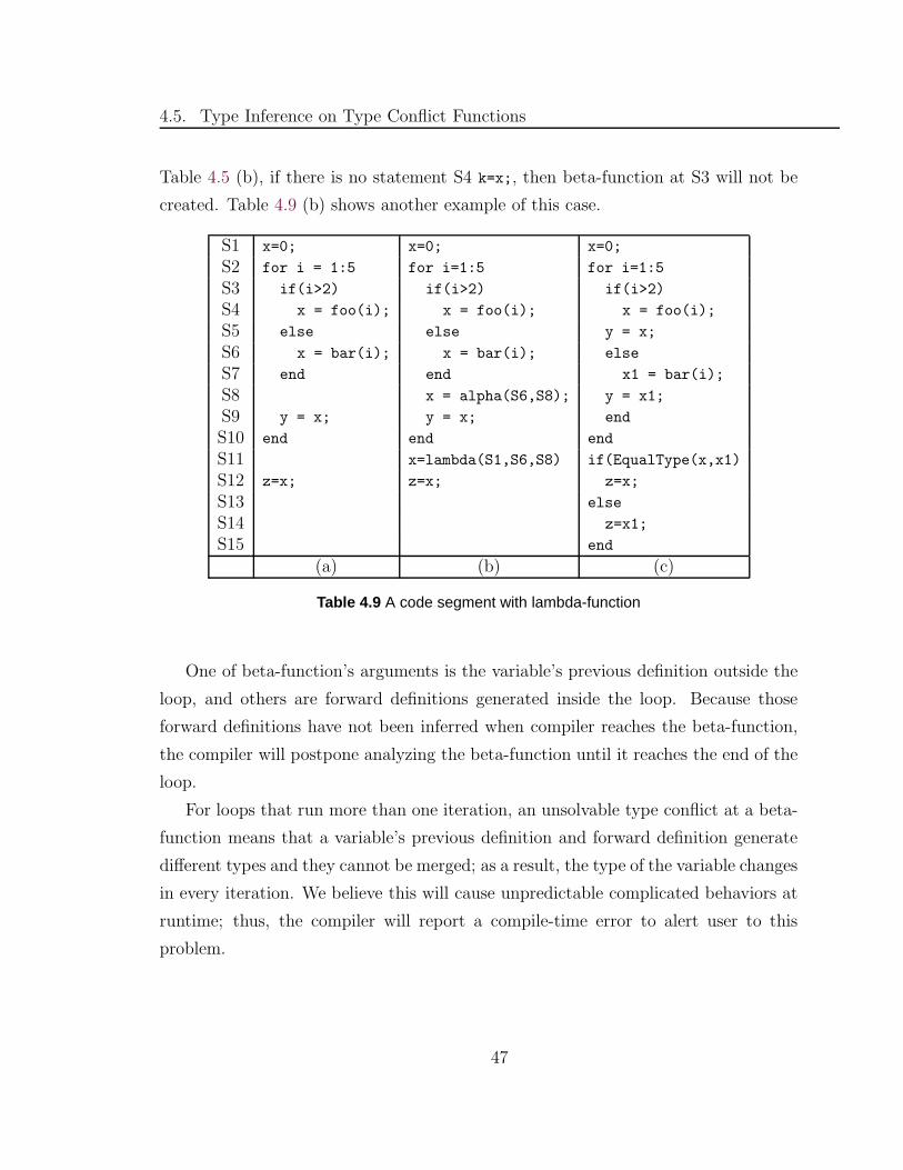
4.5. Type Inference on Type Conflict Functions
Table 4.5 (b), if there is no statement S4 k=x;, then beta-function at S3 will not be
created. Table 4.9 (b) shows another example of this case.
S1 x=0; x=0; x=0;
S2 for i = 1:5 for i=1:5 for i=1:5
S3 if(i>2) if(i>2) if(i>2)
S4 x = foo(i); x = foo(i); x = foo(i);
S5 else else y = x;
S6 x = bar(i); x = bar(i); else
S7 end end x1 = bar(i);
S8 x = alpha(S6,S8); y = x1;
S9 y = x; y = x; end
S10 end end end
S11 x=lambda(S1,S6,S8) if(EqualType(x,x1)
S12 z=x; z=x; z=x;
S13 else
S14 z=x1;
S15 end
(a) (b) (c)
Table 4.9 A code segment with lambda-function
One of beta-function’s arguments is the variable’s previous definition outside the
loop, and others are forward definitions generated inside the loop. Because those
forward definitions have not been inferred when compiler reaches the beta-function,
the compiler will postpone analyzing the beta-function until it reaches the end of the
loop.
For loops that run more than one iteration, an unsolvable type conflict at a beta-
function means that a variable’s previous definition and forward definition generate
different types and they cannot be merged; as a result, the type of the variable changes
in every iteration. We believe this will cause unpredictable complicated behaviors at
runtime; thus, the compiler will report a compile-time error to alert user to this
problem.
47
Type Inference Mechanism
4.5.3 Type Inference on Lambda-functions
The lambda-functions are located at the end of the loop, e.g., statement S13 of Table
4.5 (b) and S11 of Table 4.9 (b). They are used to monitor the changes between
the last definition before the loop and the new definitions happened inside the loop.
If a beta-function is created (e.g., statement at S3 of in Table 4.5 (b)), then the
corresponding lambda-function has the same arguments and the same behavior as
the beta-function: either they will cause a compile-time error, or be ignored because
type conflicts they had can be solved. If a beta-function is not created and the
lambda-function causes an unsolvable type conflict, then the compiler will perform
the following actions.
The compiler will create multiple versions of variables, and generate a conditional
statement to handle each version of variable at runtime using a type checking func-
tion. Each conditional block will have a copy of the following statements, which
will be renamed accordingly, and make multiple copies of the statements follow the
lambda-function, each copy represents a version of the variable and will be renamed
correspondingly.
Table 4.9 shows an example. Since the S8 in Table 4.9(b) creates a different
version of x, the compiler thus duplicates the S12, and creates an if-else-statement
(S11-S15 in Table 4.9(c)).The type checking function EqualType (x,x1) ensures the
first copy will be executed only when the type of x at that time is as same as the type
of x1. The function EqualType (x,x1) is created by compiler to determine whether
two variables have the same type based on their intrinsic types and shapes.
4.6 Value Propagation Analysis
In MATLAB, indexed array assignments (e.g., A(i)=RHS) have different meanings
according to their indices. If the indices point to a location outside the array bounds,
then the array will be expanded automatically. For example, if array A is a 3-by-3
matrix, then assignment A(4, 5)= 20 expands A to 4-by-5. In order to be able to
compare the index expression and the size of array, the compiler uses a simple value
48
4.6. Value Propagation Analysis
propagation analysis to estimate the value range of each variable and expression, and
propagate them throughout the program.
The goal of this analysis is to estimate the largest size of each array variable, and
find out which array accesses need array bounds checks. Because the goal is not to
eliminate all the array bounds checks, we used a simple approach for this analysis: it
only calculates the values of scalar variables that have one definition, and compares
values that are constant expressions. A constant expression is an expression that
contains only literals and variables which have one definition. We choose this simple
approach because it is difficult to compare expressions that contain variables that
have multiple definitions. Since our IR is not in SSA form, if a variable has multiple
definitions in a program, then it requires extra analysis to determine which value the
variable contains at a certain program point. For index expressions using variables
that have more than one definition, we add explicit array bounds checking code before
it to ensure the access is valid.
4.6.1 Calculate a Variable’s Value
For a variable that has multiple definitions in the program, we use the variable’s name
as its value. Therefore, when an expression uses those variables, we can easily find
out it is not a constant expression.
For a variable that has only one definition, its value is calculated based on the
RHS expression of its assignment. If the RHS expression is a literal, then the literal
is its value. If the RHS expression contains variables, then we apply the values of
those variables to the expression and use the result (a literal or an expression) as the
value of the variable. If the RHS expression contains functions or the expression is
too complicated to be calculated, then we use the variable’s name as its value.
For a loop variable that is assigned to a range expression, we use the first-value
and the last-value of the range expression as the minimum and maximum values of
the loop variable respectively.
49
Type Inference Mechanism
4.6.2 Compare Values
For each indexed array access, we calculate the value of each index expression and
compare it with the size of the array. There are three possible results:
1. If the array has never been defined, then use the value of index expression as
the size of the array.
2. If the two values are comparable, which means they are constant expressions
and either they are literals or they both use the same set of variables, then we
update the size of array by the larger value.
3. If the two values are not comparable, then we add array bounds checking code
in front of this statement.
Table 4.10 shows an example of using this value propagation analysis to determine
the size of array variable “A”. Table 4.10 (a) shows the MATLAB code segment, and
Figure 4.10 (b) shows the translated Fortran code. In this example, variable “n” has
two definitions (S1 and S6), so its value is itself “n”. In the for-loop, loop variable
“i” has value range [1, n], and we can derive that “x” has value range [3, 1+2*n];
therefore, the largest size of array “A” at S4 should be “1+2*n”. Because array “A”
is first defined at S4, we set the array “A” to be size “1+2*n” and add an allocation
code segment before it. At statement S7, the value of index expression is “n+1”, but
this value and the size of array are not constant expressions, because both of them
contain variable “n”, which has multiple definitions. Therefore, the two values are
not comparable. We thus add array bounds checking code in front of S7. (The array
bounds checking code will be explained in Section 4.7.2. Here we use a function,
ArrayBoundsChecking(A, [n+1]), to represent it.)
4.6.3 Additional Rule for Array Bounds Checking
We have performed flow analysis at the first step of the type inference process, and
inserted type conflict functions, each of which represents multiple definitions of a
50
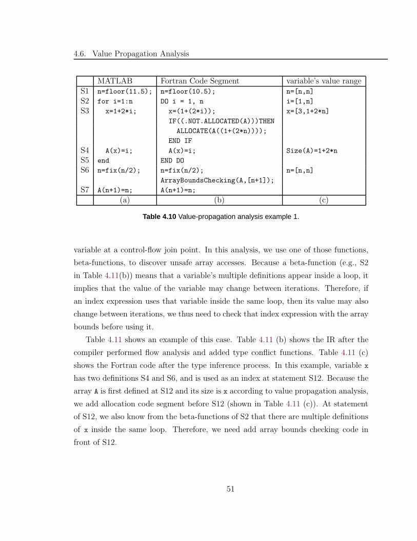
4.6. Value Propagation Analysis
MATLAB Fortran Code Segment variable’s value rangeS1 n=floor(11.5); n=floor(10.5); n=[n,n]
S2 for i=1:n DO i = 1, n i=[1,n]
S3 x=1+2*i; x=(1+(2*i)); x=[3,1+2*n]
IF((.NOT.ALLOCATED(A)))THEN
ALLOCATE(A((1+(2*n))));
END IF
S4 A(x)=i; A(x)=i; Size(A)=1+2*n
S5 end END DO
S6 n=fix(n/2); n=fix(n/2); n=[n,n]
ArrayBoundsChecking(A,[n+1]);
S7 A(n+1)=n; A(n+1)=n;
(a) (b) (c)
Table 4.10 Value-propagation analysis example 1.
variable at a control-flow join point. In this analysis, we use one of those functions,
beta-functions, to discover unsafe array accesses. Because a beta-function (e.g., S2
in Table 4.11(b)) means that a variable’s multiple definitions appear inside a loop, it
implies that the value of the variable may change between iterations. Therefore, if
an index expression uses that variable inside the same loop, then its value may also
change between iterations, we thus need to check that index expression with the array
bounds before using it.
Table 4.11 shows an example of this case. Table 4.11 (b) shows the IR after the
compiler performed flow analysis and added type conflict functions. Table 4.11 (c)
shows the Fortran code after the type inference process. In this example, variable x
has two definitions S4 and S6, and is used as an index at statement S12. Because the
array A is first defined at S12 and its size is x according to value propagation analysis,
we add allocation code segment before S12 (shown in Table 4.11 (c)). At statement
of S12, we also know from the beta-functions of S2 that there are multiple definitions
of x inside the same loop. Therefore, we need add array bounds checking code in
front of S12.
51
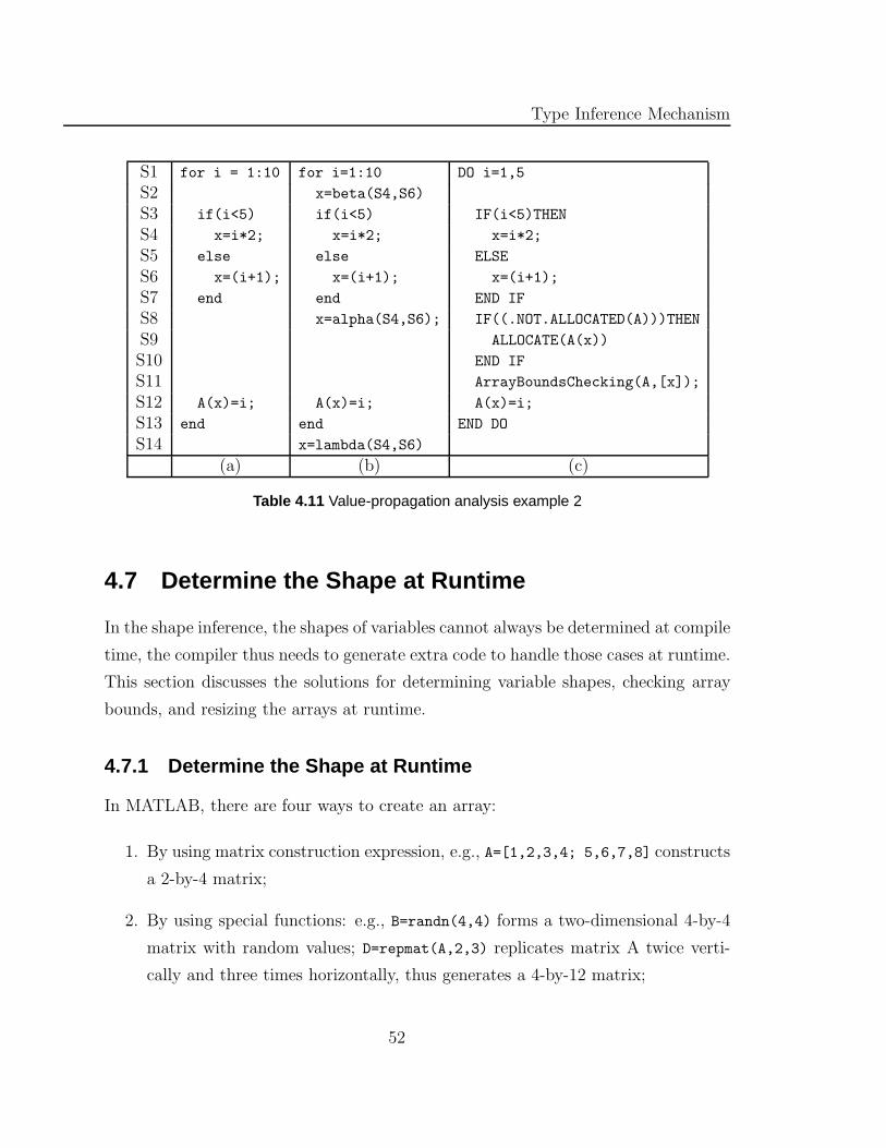
Type Inference Mechanism
S1 for i = 1:10 for i=1:10 DO i=1,5
S2 x=beta(S4,S6)
S3 if(i<5) if(i<5) IF(i<5)THEN
S4 x=i*2; x=i*2; x=i*2;
S5 else else ELSE
S6 x=(i+1); x=(i+1); x=(i+1);
S7 end end END IF
S8 x=alpha(S4,S6); IF((.NOT.ALLOCATED(A)))THEN
S9 ALLOCATE(A(x))
S10 END IF
S11 ArrayBoundsChecking(A,[x]);
S12 A(x)=i; A(x)=i; A(x)=i;
S13 end end END DO
S14 x=lambda(S4,S6)
(a) (b) (c)
Table 4.11 Value-propagation analysis example 2
4.7 Determine the Shape at Runtime
In the shape inference, the shapes of variables cannot always be determined at compile
time, the compiler thus needs to generate extra code to handle those cases at runtime.
This section discusses the solutions for determining variable shapes, checking array
bounds, and resizing the arrays at runtime.
4.7.1 Determine the Shape at Runtime
In MATLAB, there are four ways to create an array:
1. By using matrix construction expression, e.g., A=[1,2,3,4; 5,6,7,8] constructs
a 2-by-4 matrix;
2. By using special functions: e.g., B=randn(4,4) forms a two-dimensional 4-by-4
matrix with random values; D=repmat(A,2,3) replicates matrix A twice verti-
cally and three times horizontally, thus generates a 4-by-12 matrix;
52
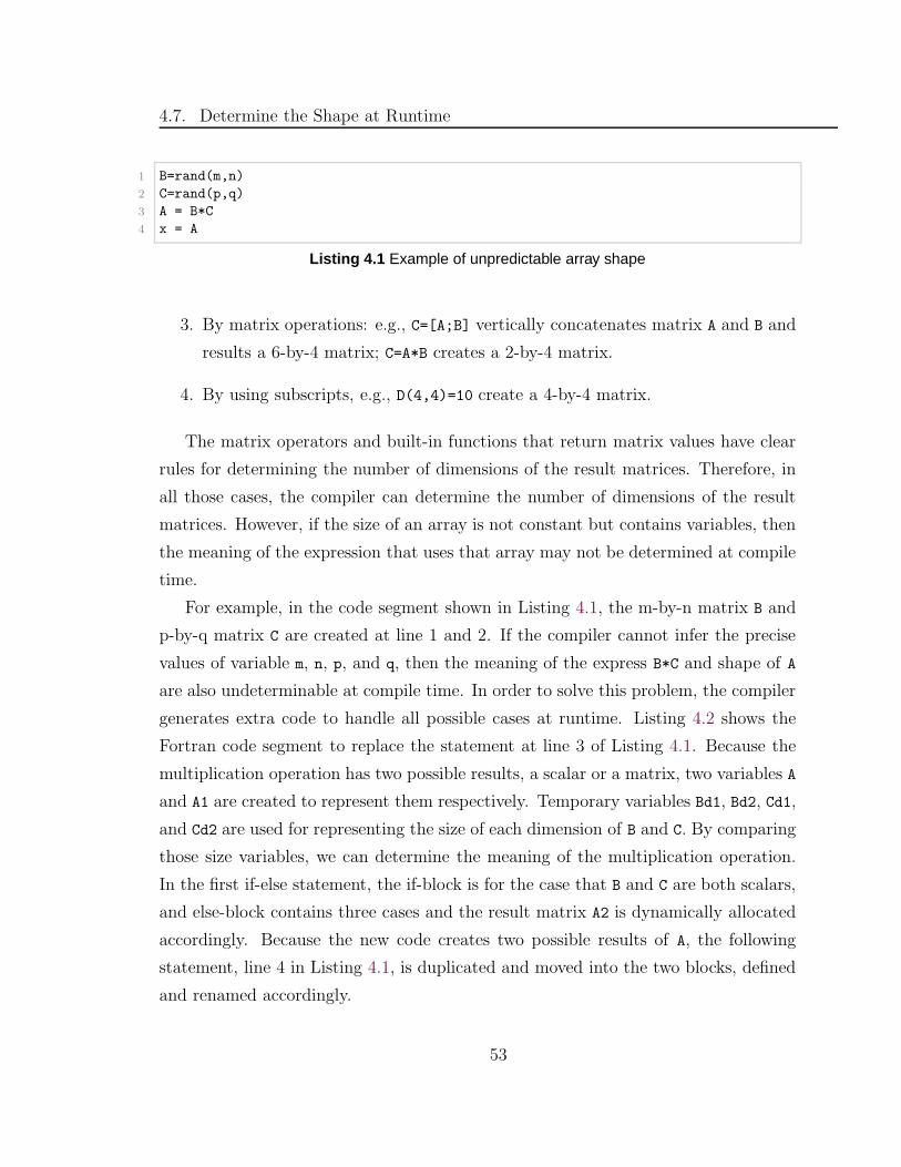
4.7. Determine the Shape at Runtime
1 B=rand(m,n)
2 C=rand(p,q)
3 A = B*C
4 x = A
Listing 4.1 Example of unpredictable array shape
3. By matrix operations: e.g., C=[A;B] vertically concatenates matrix A and B and
results a 6-by-4 matrix; C=A*B creates a 2-by-4 matrix.
4. By using subscripts, e.g., D(4,4)=10 create a 4-by-4 matrix.
The matrix operators and built-in functions that return matrix values have clear
rules for determining the number of dimensions of the result matrices. Therefore, in
all those cases, the compiler can determine the number of dimensions of the result
matrices. However, if the size of an array is not constant but contains variables, then
the meaning of the expression that uses that array may not be determined at compile
time.
For example, in the code segment shown in Listing 4.1, the m-by-n matrix B and
p-by-q matrix C are created at line 1 and 2. If the compiler cannot infer the precise
values of variable m, n, p, and q, then the meaning of the express B*C and shape of A
are also undeterminable at compile time. In order to solve this problem, the compiler
generates extra code to handle all possible cases at runtime. Listing 4.2 shows the
Fortran code segment to replace the statement at line 3 of Listing 4.1. Because the
multiplication operation has two possible results, a scalar or a matrix, two variables A
and A1 are created to represent them respectively. Temporary variables Bd1, Bd2, Cd1,
and Cd2 are used for representing the size of each dimension of B and C. By comparing
those size variables, we can determine the meaning of the multiplication operation.
In the first if-else statement, the if-block is for the case that B and C are both scalars,
and else-block contains three cases and the result matrix A2 is dynamically allocated
accordingly. Because the new code creates two possible results of A, the following
statement, line 4 in Listing 4.1, is duplicated and moved into the two blocks, defined
and renamed accordingly.
53
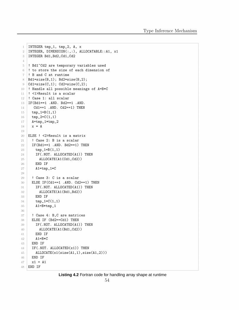
Type Inference Mechanism
1 INTEGER tmp_1, tmp_2, A, x
2 INTEGER, DIMENSION(:,:), ALLOCATABLE::A1, x1
3 INTEGER Bd1,Bd2,Cd1,Cd2
4
5 ! Bd1~Cd2 are temporary variables used
6 ! to store the size of each dimension of
7 ! B and C at runtime
8 Bd1=size(B,1); Bd2=size(B,2);
9 Cd1=size(C,1); Cd2=size(C,2);
10 ! Handle all possible meanings of A=B*C
11 ! <1>Result is a scalar
12 ! Case 1: all scalar
13 IF(Bd1==1 .AND. Bd2==1 .AND.
14 Cd1==1 .AND. Cd2==1) THEN
15 tmp_1=B(1,1)
16 tmp_2=C(1,1)
17 A=tmp_1*tmp_2
18 x = A
19
20 ELSE ! <2>Result is a matrix
21 ! Case 2: B is a scalar
22 IF(Bd1==1 .AND. Bd2==1) THEN
23 tmp_1=B(1,1)
24 IF(.NOT. ALLOCATED(A1)) THEN
25 ALLOCATE(A1(Cd1,Cd2))
26 END IF
27 A1=tmp_1*C
28
29 ! Case 3: C is a scalar
30 ELSE IF(Cd1==1 .AND. Cd2==1) THEN
31 IF(.NOT. ALLOCATED(A1)) THEN
32 ALLOCATE(A1(Bd1,Bd2))
33 END IF
34 tmp_1=C(1,1)
35 A1=B*tmp_1
36
37 ! Case 4: B,C are matrices
38 ELSE IF (Bd2==Cd1) THEN
39 IF(.NOT. ALLOCATED(A1)) THEN
40 ALLOCATE(A1(Bd1,Cd2))
41 END IF
42 A1=B*C
43 END IF
44 IF(.NOT. ALLOCATED(x1)) THEN
45 ALLOCATE(x1(size(A1,1),size(A1,2)))
46 END IF
47 x1 = A1
48 END IF
Listing 4.2 Fortran code for handling array shape at runtime54
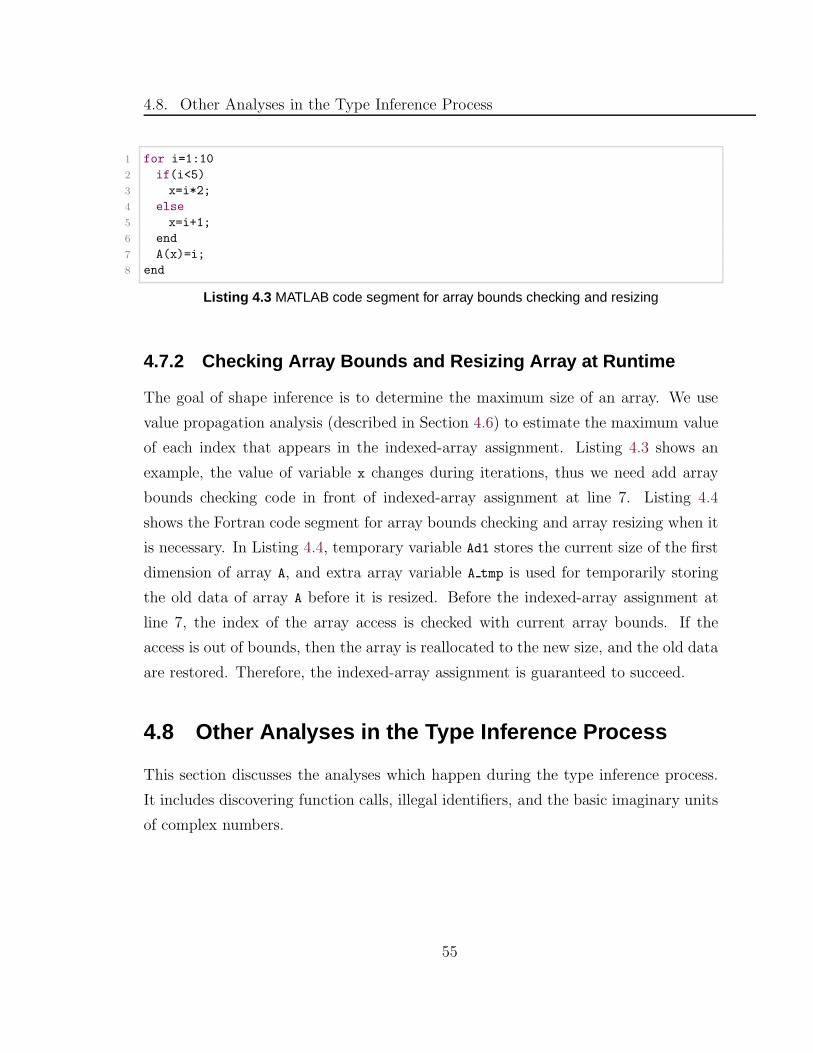
4.8. Other Analyses in the Type Inference Process
1 for i=1:10
2 if(i<5)
3 x=i*2;
4 else
5 x=i+1;
6 end
7 A(x)=i;
8 end
Listing 4.3 MATLAB code segment for array bounds checking and resizing
4.7.2 Checking Array Bounds and Resizing Array at Runtime
The goal of shape inference is to determine the maximum size of an array. We use
value propagation analysis (described in Section 4.6) to estimate the maximum value
of each index that appears in the indexed-array assignment. Listing 4.3 shows an
example, the value of variable x changes during iterations, thus we need add array
bounds checking code in front of indexed-array assignment at line 7. Listing 4.4
shows the Fortran code segment for array bounds checking and array resizing when it
is necessary. In Listing 4.4, temporary variable Ad1 stores the current size of the first
dimension of array A, and extra array variable A tmp is used for temporarily storing
the old data of array A before it is resized. Before the indexed-array assignment at
line 7, the index of the array access is checked with current array bounds. If the
access is out of bounds, then the array is reallocated to the new size, and the old data
are restored. Therefore, the indexed-array assignment is guaranteed to succeed.
4.8 Other Analyses in the Type Inference Process
This section discusses the analyses which happen during the type inference process.
It includes discovering function calls, illegal identifiers, and the basic imaginary units
of complex numbers.
55
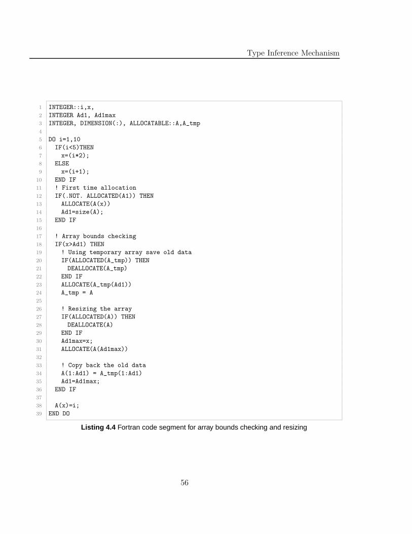
Type Inference Mechanism
1 INTEGER::i,x,
2 INTEGER Ad1, Ad1max
3 INTEGER, DIMENSION(:), ALLOCATABLE::A,A_tmp
4
5 DO i=1,10
6 IF(i<5)THEN
7 x=(i*2);
8 ELSE
9 x=(i+1);
10 END IF
11 ! First time allocation
12 IF(.NOT. ALLOCATED(A1)) THEN
13 ALLOCATE(A(x))
14 Ad1=size(A);
15 END IF
16
17 ! Array bounds checking
18 IF(x>Ad1) THEN
19 ! Using temporary array save old data
20 IF(ALLOCATED(A_tmp)) THEN
21 DEALLOCATE(A_tmp)
22 END IF
23 ALLOCATE(A_tmp(Ad1))
24 A_tmp = A
25
26 ! Resizing the array
27 IF(ALLOCATED(A)) THEN
28 DEALLOCATE(A)
29 END IF
30 Ad1max=x;
31 ALLOCATE(A(Ad1max))
32
33 ! Copy back the old data
34 A(1:Ad1) = A_tmp(1:Ad1)
35 Ad1=Ad1max;
36 END IF
37
38 A(x)=i;
39 END DO
Listing 4.4 Fortran code segment for array bounds checking and resizing
56
4.8. Other Analyses in the Type Inference Process
4.8.1 Discover Identifiers That are not Variables
After solving the script calls, an identifier appearing in the program could be a variable
or a function call as discussed in Section 3.2.2. Whether an identifier is a variable or
a function call is determined during the type inference process.
Before performing type inference, a symbol table has been created for each user-
defined function; all variables, including input and output parameters, in the symbol
table are initialized to have empty type. When the type inference reaches a user-
defined function, the types of input parameters of that function will be updated
based on the calling context.
Type inference traverses each node of a function’s AST from top to bottom. For
every statement, it gathers the use list of the statement, and checks each identifier
which appears in the use list to determine whether it is a variable or not based on
the following rules:
1. If the identifier has an entry in the symbol table and the type stored in that
entry is not empty type, then the identifier is a variable.
2. If the identifier has an entry in the symbol table but the type stored in that
entry is empty type, then there are two possibilities: if its name is included in
the list of built-in functions and user-defined functions, then the compiler will
treat it as a function call and raise an warning; otherwise, it is an uninitialized
variable and the compiler will raise an error.
3. If the identifier has no entry in the symbol table, then there are two possibilities:
if its name is included in the list of built-in functions and user-defined functions,
then it is a function call; otherwise, it is an undefined variable and the compiler
will raise an error.
4.8.2 Discover the Basic Imaginary Unit of Complex Numbers
MATLAB has a convenient way to declare complex constants. For example, a complex
number with a real part of 2 and an imaginary part of 3 could be expressed as 2+3i,
57
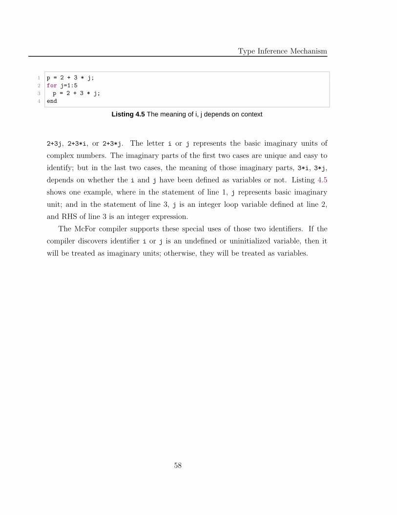
Type Inference Mechanism
1 p = 2 + 3 * j;
2 for j=1:5
3 p = 2 + 3 * j;
4 end
Listing 4.5 The meaning of i, j depends on context
2+3j, 2+3*i, or 2+3*j. The letter i or j represents the basic imaginary units of
complex numbers. The imaginary parts of the first two cases are unique and easy to
identify; but in the last two cases, the meaning of those imaginary parts, 3*i, 3*j,
depends on whether the i and j have been defined as variables or not. Listing 4.5
shows one example, where in the statement of line 1, j represents basic imaginary
unit; and in the statement of line 3, j is an integer loop variable defined at line 2,
and RHS of line 3 is an integer expression.
The McFor compiler supports these special uses of those two identifiers. If the
compiler discovers identifier i or j is an undefined or uninitialized variable, then it
will be treated as imaginary units; otherwise, they will be treated as variables.
58
Chapter 5
Transformations
Fortran is the closest conventional language to MATLAB because it uses the
same array syntax and has similar semantics for most array operations. However,
MATLAB has many special features that Fortran does not support. For example,
MATLAB supports linear indexing and using arrays as indices; it has various ways
of constructing arrays; and its operators can take operands of any type. We thus
designed an extra transformation phase to transform those special statements into
functional equivalent forms that can be straightforwardly translated into Fortran by
the code generator. This chapter discusses transformations designed for those special
features, which include transformations for array constructions (Section 5.1), linear
indexing (Section 5.2), using arrays as indices (Section 5.3), and type conversion (Sec-
tion 5.4). Generating readable Fortran code is another goal of the McFor compiler.
The aggregation transformation is designed for this purpose; it is discussed in Section
5.5.
5.1 Transformations for Array Constructions
MATLAB has a very powerful operator [] for building arrays. This brackets operator
is used as array constructor operator for creating a multi-dimensional array in one
assignment, e.g., A=[1,2,3,4; 5,6,7,8] constructs a 2-by-4 matrix. It is also served
59
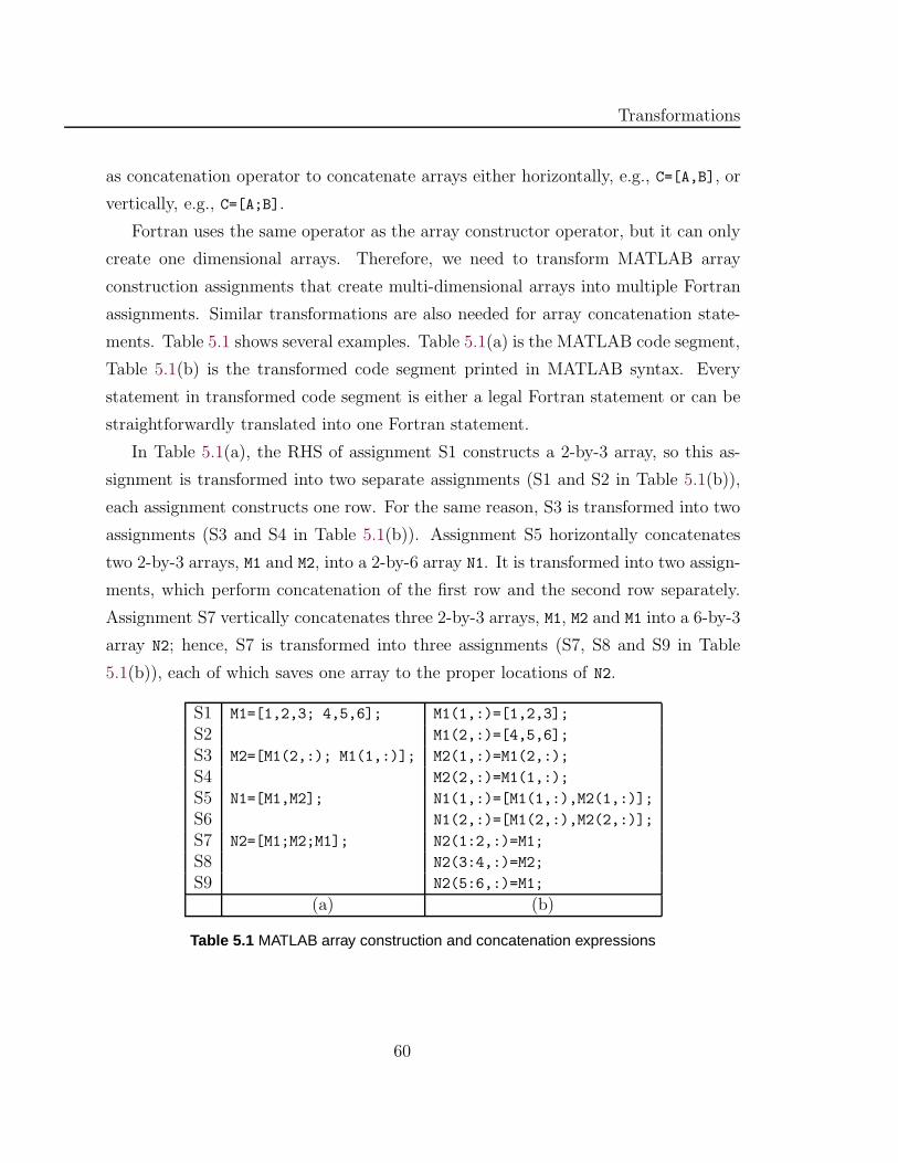
Transformations
as concatenation operator to concatenate arrays either horizontally, e.g., C=[A,B], or
vertically, e.g., C=[A;B].
Fortran uses the same operator as the array constructor operator, but it can only
create one dimensional arrays. Therefore, we need to transform MATLAB array
construction assignments that create multi-dimensional arrays into multiple Fortran
assignments. Similar transformations are also needed for array concatenation state-
ments. Table 5.1 shows several examples. Table 5.1(a) is the MATLAB code segment,
Table 5.1(b) is the transformed code segment printed in MATLAB syntax. Every
statement in transformed code segment is either a legal Fortran statement or can be
straightforwardly translated into one Fortran statement.
In Table 5.1(a), the RHS of assignment S1 constructs a 2-by-3 array, so this as-
signment is transformed into two separate assignments (S1 and S2 in Table 5.1(b)),
each assignment constructs one row. For the same reason, S3 is transformed into two
assignments (S3 and S4 in Table 5.1(b)). Assignment S5 horizontally concatenates
two 2-by-3 arrays, M1 and M2, into a 2-by-6 array N1. It is transformed into two assign-
ments, which perform concatenation of the first row and the second row separately.
Assignment S7 vertically concatenates three 2-by-3 arrays, M1, M2 and M1 into a 6-by-3
array N2; hence, S7 is transformed into three assignments (S7, S8 and S9 in Table
5.1(b)), each of which saves one array to the proper locations of N2.
S1 M1=[1,2,3; 4,5,6]; M1(1,:)=[1,2,3];
S2 M1(2,:)=[4,5,6];
S3 M2=[M1(2,:); M1(1,:)]; M2(1,:)=M1(2,:);
S4 M2(2,:)=M1(1,:);
S5 N1=[M1,M2]; N1(1,:)=[M1(1,:),M2(1,:)];
S6 N1(2,:)=[M1(2,:),M2(2,:)];
S7 N2=[M1;M2;M1]; N2(1:2,:)=M1;
S8 N2(3:4,:)=M2;
S9 N2(5:6,:)=M1;
(a) (b)
Table 5.1 MATLAB array construction and concatenation expressions
60
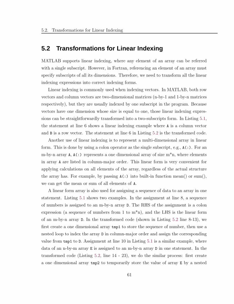
5.2. Transformations for Linear Indexing
5.2 Transformations for Linear Indexing
MATLAB supports linear indexing, where any element of an array can be referred
with a single subscript. However, in Fortran, referencing an element of an array must
specify subscripts of all its dimensions. Therefore, we need to transform all the linear
indexing expressions into correct indexing forms.
Linear indexing is commonly used when indexing vectors. In MATLAB, both row
vectors and column vectors are two-dimensional matrices (n-by-1 and 1-by-n matrices
respectively), but they are usually indexed by one subscript in the program. Because
vectors have one dimension whose size is equal to one, those linear indexing expres-
sions can be straightforwardly transformed into a two-subscripts form. In Listing 5.1,
the statement at line 6 shows a linear indexing example where A is a column vector
and B is a row vector. The statement at line 6 in Listing 5.2 is the transformed code.
Another use of linear indexing is to represent a multi-dimensional array in linear
form. This is done by using a colon operator as the single subscript, e.g., A(:). For an
m-by-n array A, A(:) represents a one dimensional array of size m*n, where elements
in array A are listed in column-major order. This linear form is very convenient for
applying calculations on all elements of the array, regardless of the actual structure
the array has. For example, by passing A(:) into built-in function mean() or sum(),
we can get the mean or sum of all elements of A.
A linear form array is also used for assigning a sequence of data to an array in one
statement. Listing 5.1 shows two examples. In the assignment at line 8, a sequence
of numbers is assigned to an m-by-n array D. The RHS of the assignment is a colon
expression (a sequence of numbers from 1 to m*n), and the LHS is the linear form
of an m-by-n array D. In the transformed code (shown in Listing 5.2 line 8-13), we
first create a one dimensional array tmp1 to store the sequence of number, then use a
nested loop to index the array D in column-major order and assign the corresponding
value from tmp1 to D. Assignment at line 10 in Listing 5.1 is a similar example, where
data of an n-by-m array E is assigned to an m-by-n array D in one statement. In the
transformed code (Listing 5.2, line 14 - 23), we do the similar process: first create
a one dimensional array tmp2 to temporarily store the value of array E by a nested
61
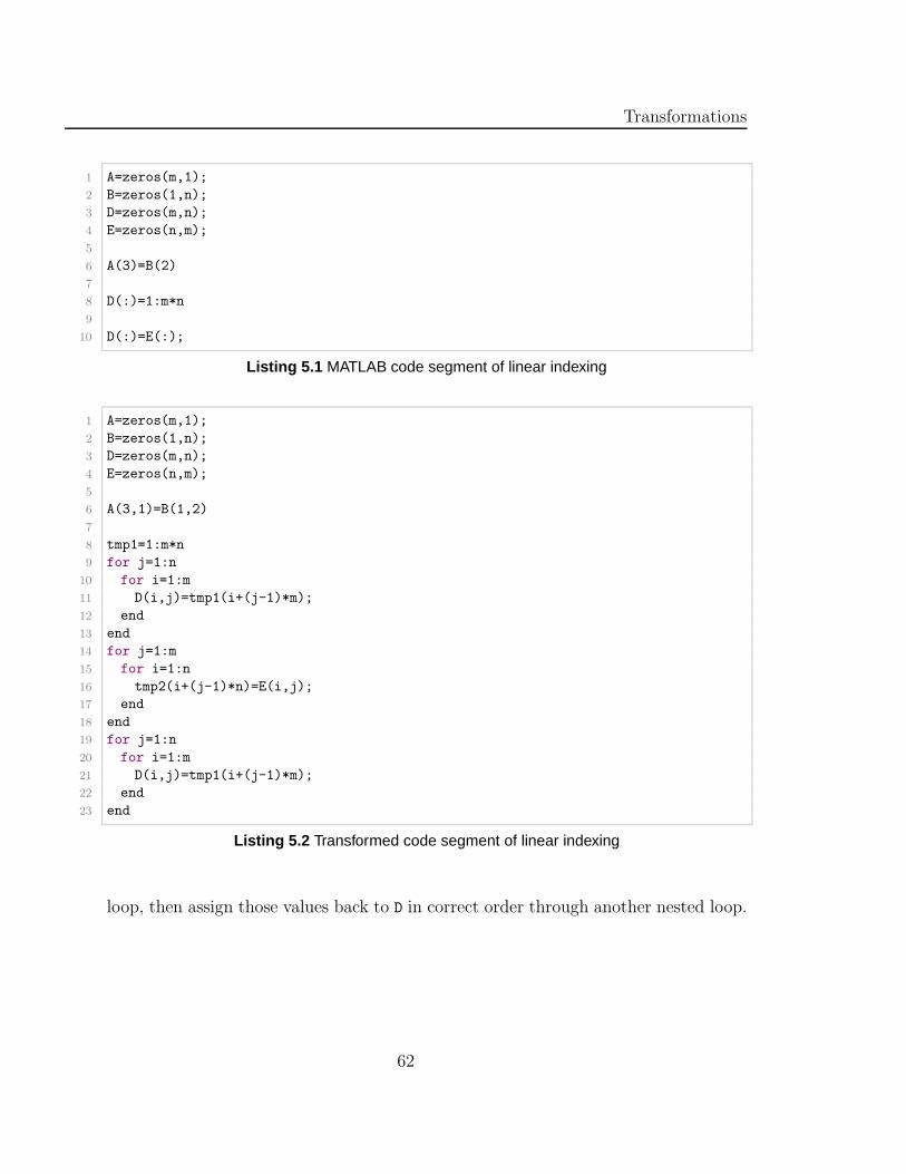
Transformations
1 A=zeros(m,1);
2 B=zeros(1,n);
3 D=zeros(m,n);
4 E=zeros(n,m);
5
6 A(3)=B(2)
7
8 D(:)=1:m*n
9
10 D(:)=E(:);
Listing 5.1 MATLAB code segment of linear indexing
1 A=zeros(m,1);
2 B=zeros(1,n);
3 D=zeros(m,n);
4 E=zeros(n,m);
5
6 A(3,1)=B(1,2)
7
8 tmp1=1:m*n
9 for j=1:n
10 for i=1:m
11 D(i,j)=tmp1(i+(j-1)*m);
12 end
13 end
14 for j=1:m
15 for i=1:n
16 tmp2(i+(j-1)*n)=E(i,j);
17 end
18 end
19 for j=1:n
20 for i=1:m
21 D(i,j)=tmp1(i+(j-1)*m);
22 end
23 end
Listing 5.2 Transformed code segment of linear indexing
loop, then assign those values back to D in correct order through another nested loop.
62
5.3. Transformations for Using Arrays as Indices
5.3 Transformations for Using Arrays as Indices
In MATLAB, logical arrays or integer arrays can be used as indices of another arrays.
If an integer array is used as an index, then the values of its elements are used
as subscripts for the indexed array; therefore, the values of all its elements must be
positive integers and must not exceed the size of the indexed array. For example, if D
is [1,3;2,4] and A is another array, then A(D) represents A(1), A(2), A(3), and A(4),
(elements of D are listed in linear indexing form). If A is a 2-by-3 array, then the value
of any element in D should not bigger than 6.
Listing 5.3 and Listings 5.4 shows two examples. In Listing 5.3, at the LHS of
assignment of line 5, integer array D is used as the index for array R. In the trans-
formed code (Listing 5.4, lines 5-11), we create a nested loop to get the value of every
element of D, and convert them into corresponding indices of array R, and perform
the assignment on that element. At assignment of line 7 of Listing 5.3, the same
indexed expression is used at the RHS, and the LHS is a linear form array E. For this
assignment, we use the technique for transforming linear indexing. As shown in the
transformed code (Listing 5.4, line 12-24), we first create a temporary array tmp1 to
save the value of R(D) by using a nested loop, then assign them back to E in correct
order through another nested loop.
When a logical array is used as an index, it has a different meaning: the positions
of the true values in the logical array will become the indices for the indexed array.
For example, if logical array B is [true, false; false, true], and array A has the
same shape as B, then A(B) represents A(1,1), A(2,2). Table 5.2 shows an example of
using logical array as an index. In MATLAB code segment (Table 5.2(a)), variable A
is an m-by-n array, and B is a logical array of the same shape. In the transformed code
segment (Table 5.2(b)), assignment S3 of Table 5.2(a) is transformed into a nested
loop that goes through every element of array A and B in column-major order. Inside
the loop, an extra if-statement checks the element of B to see whether its value is true
or false, and updates the element of A when that value is true.
63
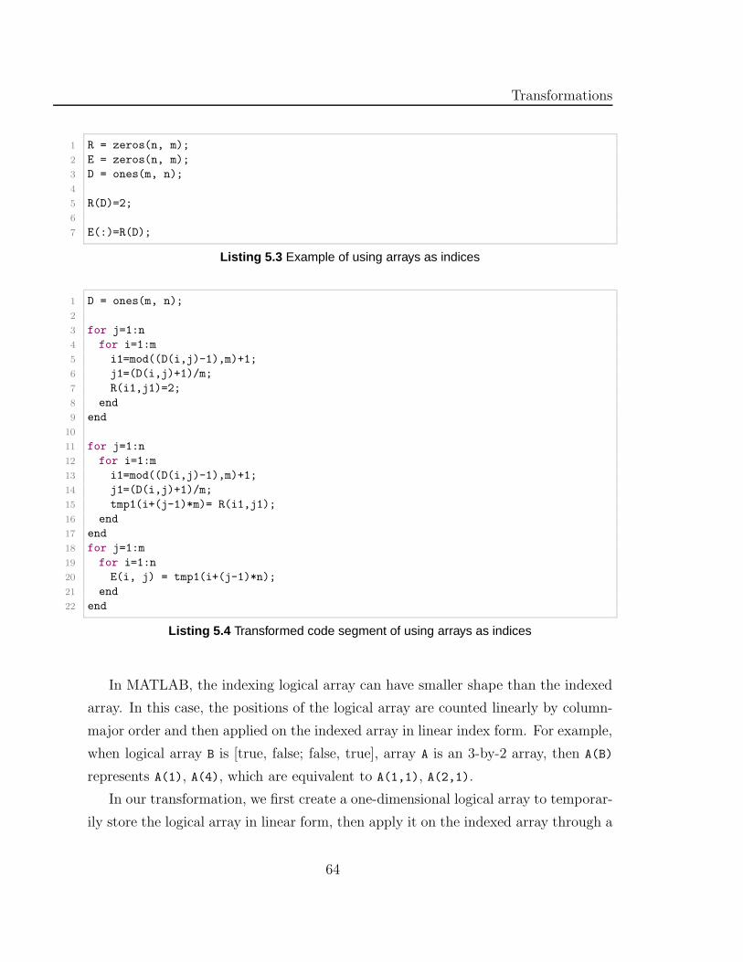
Transformations
1 R = zeros(n, m);
2 E = zeros(n, m);
3 D = ones(m, n);
4
5 R(D)=2;
6
7 E(:)=R(D);
Listing 5.3 Example of using arrays as indices
1 D = ones(m, n);
2
3 for j=1:n
4 for i=1:m
5 i1=mod((D(i,j)-1),m)+1;
6 j1=(D(i,j)+1)/m;
7 R(i1,j1)=2;
8 end
9 end
10
11 for j=1:n
12 for i=1:m
13 i1=mod((D(i,j)-1),m)+1;
14 j1=(D(i,j)+1)/m;
15 tmp1(i+(j-1)*m)= R(i1,j1);
16 end
17 end
18 for j=1:m
19 for i=1:n
20 E(i, j) = tmp1(i+(j-1)*n);
21 end
22 end
Listing 5.4 Transformed code segment of using arrays as indices
In MATLAB, the indexing logical array can have smaller shape than the indexed
array. In this case, the positions of the logical array are counted linearly by column-
major order and then applied on the indexed array in linear index form. For example,
when logical array B is [true, false; false, true], array A is an 3-by-2 array, then A(B)
represents A(1), A(4), which are equivalent to A(1,1), A(2,1).
In our transformation, we first create a one-dimensional logical array to temporar-
ily store the logical array in linear form, then apply it on the indexed array through a
64
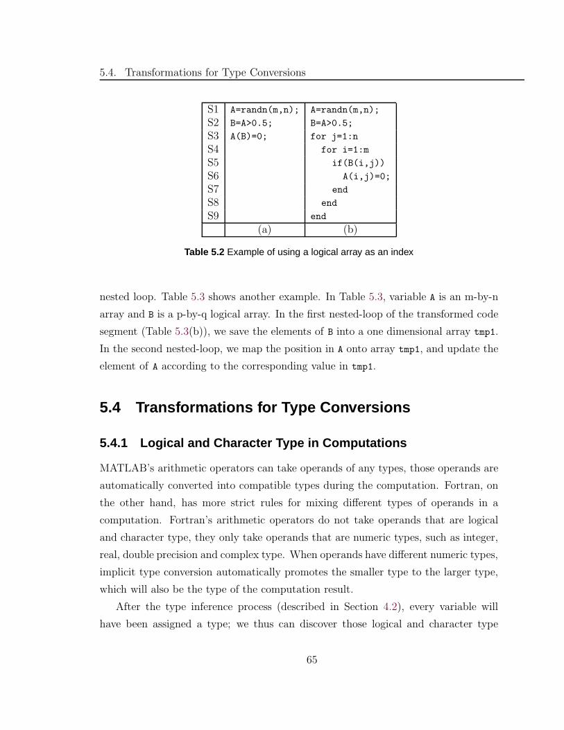
5.4. Transformations for Type Conversions
S1 A=randn(m,n); A=randn(m,n);
S2 B=A>0.5; B=A>0.5;
S3 A(B)=0; for j=1:n
S4 for i=1:m
S5 if(B(i,j))
S6 A(i,j)=0;
S7 end
S8 end
S9 end
(a) (b)
Table 5.2 Example of using a logical array as an index
nested loop. Table 5.3 shows another example. In Table 5.3, variable A is an m-by-n
array and B is a p-by-q logical array. In the first nested-loop of the transformed code
segment (Table 5.3(b)), we save the elements of B into a one dimensional array tmp1.
In the second nested-loop, we map the position in A onto array tmp1, and update the
element of A according to the corresponding value in tmp1.
5.4 Transformations for Type Conversions
5.4.1 Logical and Character Type in Computations
MATLAB’s arithmetic operators can take operands of any types, those operands are
automatically converted into compatible types during the computation. Fortran, on
the other hand, has more strict rules for mixing different types of operands in a
computation. Fortran’s arithmetic operators do not take operands that are logical
and character type, they only take operands that are numeric types, such as integer,
real, double precision and complex type. When operands have different numeric types,
implicit type conversion automatically promotes the smaller type to the larger type,
which will also be the type of the computation result.
After the type inference process (described in Section 4.2), every variable will
have been assigned a type; we thus can discover those logical and character type
65
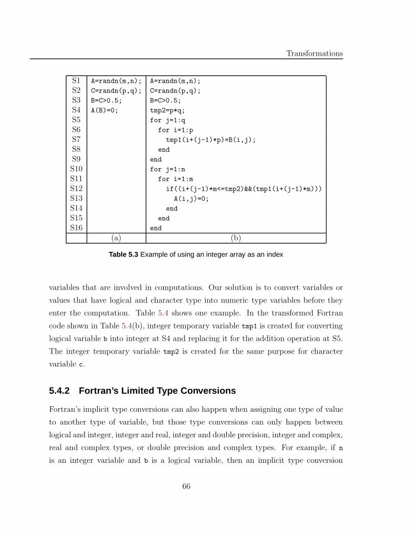
Transformations
S1 A=randn(m,n); A=randn(m,n);
S2 C=randn(p,q); C=randn(p,q);
S3 B=C>0.5; B=C>0.5;
S4 A(B)=0; tmp2=p*q;
S5 for j=1:q
S6 for i=1:p
S7 tmp1(i+(j-1)*p)=B(i,j);
S8 end
S9 end
S10 for j=1:n
S11 for i=1:m
S12 if((i+(j-1)*m<=tmp2)&&(tmp1(i+(j-1)*m)))
S13 A(i,j)=0;
S14 end
S15 end
S16 end
(a) (b)
Table 5.3 Example of using an integer array as an index
variables that are involved in computations. Our solution is to convert variables or
values that have logical and character type into numeric type variables before they
enter the computation. Table 5.4 shows one example. In the transformed Fortran
code shown in Table 5.4(b), integer temporary variable tmp1 is created for converting
logical variable b into integer at S4 and replacing it for the addition operation at S5.
The integer temporary variable tmp2 is created for the same purpose for character
variable c.
5.4.2 Fortran’s Limited Type Conversions
Fortran’s implicit type conversions can also happen when assigning one type of value
to another type of variable, but those type conversions can only happen between
logical and integer, integer and real, integer and double precision, integer and complex,
real and complex types, or double precision and complex types. For example, if n
is an integer variable and b is a logical variable, then an implicit type conversion
66
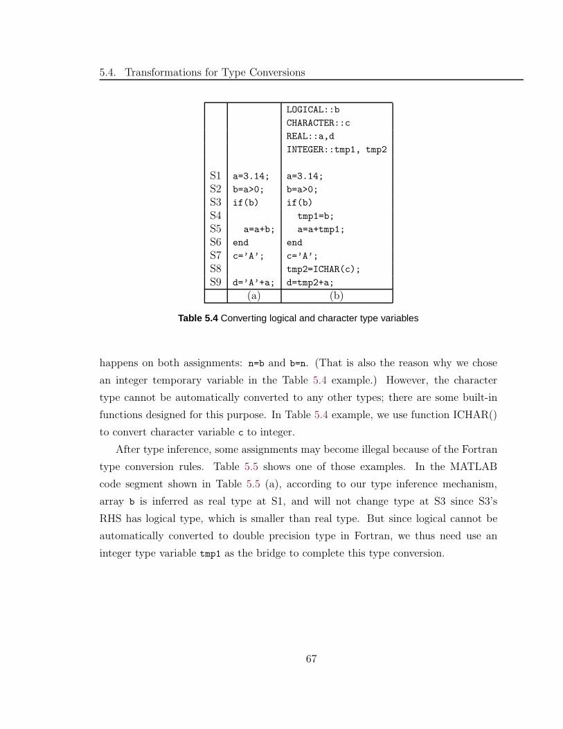
5.4. Transformations for Type Conversions
LOGICAL::b
CHARACTER::c
REAL::a,d
INTEGER::tmp1, tmp2
S1 a=3.14; a=3.14;
S2 b=a>0; b=a>0;
S3 if(b) if(b)
S4 tmp1=b;
S5 a=a+b; a=a+tmp1;
S6 end end
S7 c=’A’; c=’A’;
S8 tmp2=ICHAR(c);
S9 d=’A’+a; d=tmp2+a;
(a) (b)
Table 5.4 Converting logical and character type variables
happens on both assignments: n=b and b=n. (That is also the reason why we chose
an integer temporary variable in the Table 5.4 example.) However, the character
type cannot be automatically converted to any other types; there are some built-in
functions designed for this purpose. In Table 5.4 example, we use function ICHAR()
to convert character variable c to integer.
After type inference, some assignments may become illegal because of the Fortran
type conversion rules. Table 5.5 shows one of those examples. In the MATLAB
code segment shown in Table 5.5 (a), according to our type inference mechanism,
array b is inferred as real type at S1, and will not change type at S3 since S3’s
RHS has logical type, which is smaller than real type. But since logical cannot be
automatically converted to double precision type in Fortran, we thus need use an
integer type variable tmp1 as the bridge to complete this type conversion.
67
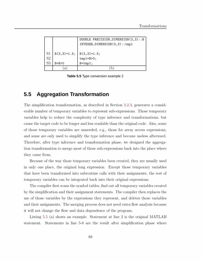
Transformations
DOUBLE PRECISION,DIMENSION(3,3)::B
INTEGER,DIMENSION(3,3)::tmp1
S1 B(3,3)=1.5; B(3,3)=1.5;
S2 tmp1=B>0;
S3 B=B>0 B=tmp1;
(a) (b)
Table 5.5 Type conversion example 2
5.5 Aggregation Transformation
The simplification transformation, as described in Section 3.2.3, generates a consid-
erable number of temporary variables to represent sub-expressions. Those temporary
variables help to reduce the complexity of type inference and transformations, but
cause the target code to be longer and less readable than the original code. Also, some
of those temporary variables are unneeded, e.g., those for array access expressions,
and some are only used to simplify the type inference and become useless afterward.
Therefore, after type inference and transformation phase, we designed the aggrega-
tion transformation to merge most of those sub-expressions back into the place where
they came from.
Because of the way those temporary variables been created, they are usually used
in only one place, the original long expression. Except those temporary variables
that have been transformed into subroutine calls with their assignments, the rest of
temporary variables can be integrated back into their original expressions.
The compiler first scans the symbol tables, find out all temporary variables created
by the simplification and their assignment statements. The compiler then replaces the
use of those variables by the expressions they represent, and deletes those variables
and their assignments. The merging process does not need extra flow analysis because
it will not change the flow and data dependence of the program.
Listing 5.5 (a) shows an example. Statement at line 2 is the original MATLAB
statement. Statements in line 5-8 are the result after simplification phase where
68
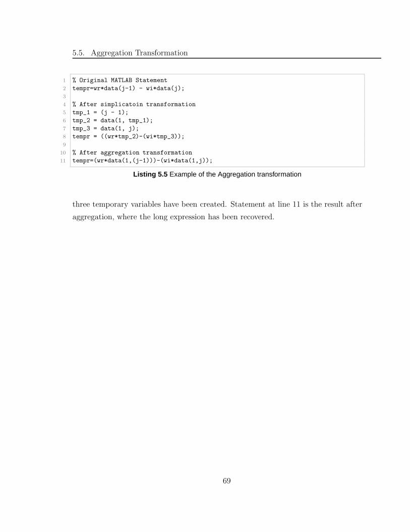
5.5. Aggregation Transformation
1 % Original MATLAB Statement
2 tempr=wr*data(j-1) - wi*data(j);
3
4 % After simplicatoin transformation
5 tmp_1 = (j - 1);
6 tmp_2 = data(1, tmp_1);
7 tmp_3 = data(1, j);
8 tempr = ((wr*tmp_2)-(wi*tmp_3));
9
10 % After aggregation transformation
11 tempr=(wr*data(1,(j-1)))-(wi*data(1,j));
Listing 5.5 Example of the Aggregation transformation
three temporary variables have been created. Statement at line 11 is the result after
aggregation, where the long expression has been recovered.
69

Transformations
70
Chapter 6
Performance Evaluation
In this chapter we present the experimental results of our McFor compiler. We
translate a set of benchmarks to measure the effectiveness of the type inference and
transformation techniques described in this thesis. The performance of compiled
codes are compared with the execution times of their corresponding MATLAB codes
in MATLAB, Octave, and McVM1 [CBHV10].
6.1 Description of the Benchmarks
This set of benchmarks is acquired from a variety of sources, some of them are used
by other MATLAB compiler projects, including FALCON [RP99, RP96], OTTER
[QMSZ98], and MAT2C [Joi03a]. We have adjusted the problem size of each bench-
mark, (including the size of array and the number of iterations), in order to get a
measurable execution time. A brief description of the benchmarks is presented below.
adpt is an implementation of finding the adaptive quadrature using Simpson’s rule.
The benchmark integrates the function∫
−1
6f(x) = 13(x − x2)e−1.5x to a tol-
erance of 4 × 10⁻¹³. This benchmark features an array whose size cannot be
predicted by the compiler and expands dynamically during the computation. It
is a benchmark from the FALCON project.
1http://www.sable.mcgill.ca/mclab/mcvm mcjit.html
71
Performance Evaluation
capr is an implementation of computing the capacitance of a transmission line using
finite difference and Gauss-Seidel method. It is a loop-based program that
involves two small matrices and performs elementary scalar operations on them.
It is from Chalmers University of Technology2.
clos calculates the transitive closure of a directed graph. Its execution time is dom-
inated by a matrix multiplication between two 450 x 450 matrices. It is a
benchmark from the OTTER [QMSZ98] project.
crni is an implementation of the Crank-Nicholson solution to the heat equation.
It is a loop-based program that performs elementary scalar operations on a
two-dimensional matrix (2300 x 2300). It is a benchmark from the FALCON
project.
dich is an implementation of the Dirichlet solution to Laplace’s equation. It is a loop-
based program that performs elementary scalar operations on a two-dimensional
matrix (134 x 134). It is a benchmark from the FALCON project.
diff calculates the diffraction pattern of monochromatic light through a transmission
grating for two slits. It is a loop-based program that performs calculations
on scalar variables and saves the results into an array whose size is increased
dynamically. It is from “The MathWorks’ Central File Exchange”. 3
edit calculates the edit distance between two strings. Its major computation is a
character comparison, which compares every character of one string with all
the characters of another string, and saves the result into a two-dimensional
array. It is from “The MathWorks’ Central File Exchange”.
fdtd is an implementation of applying the Finite Difference Time Domain (FDTD)
technique on a hexahedral cavity with conducting walls. It is a loop-based
program that performs computations on multiple elements between six three-
dimensional arrays. It is from Chalmers University of Technology.
2http://www.elmagn.chalmers.se/courses/CEM/3http://www.mathworks.com/matlabcentral/fileexchange
72
6.2. Performance Results
fft computes the discrete Fourier transform for complex data. It is a loop-based
program that performs elementary scalar operations on a one dimension array.
This is our implementation of the algorithm from book “Numerical Recipes”
[WPF07].
fiff is an implementation of finite-difference solution to the wave equation. It is
a loop-based program, and performs elementary scalar operations on a two-
dimensional array. It is a benchmark from the FALCON project.
mbrt computes mandelbrot set with specified number elements and number of iter-
ations. It is a loop-based program that performs elementary scalar operations
on complex type data. It is written by Anton Dubrau of McLab team.
nb1d is an implementation of N-body simulation using one-dimensional arrays. It is
a loop-based program that involves various vector-vector computations. It is a
benchmark of OTTER project.
nb3d is an implementation of N-body simulation using three-dimension arrays. It
involves various matrix-matrix element-wise computations and several special
cases of indexing by an array. It is a benchmark of OTTER project.
These benchmarks only use the features supported by McFor. Thus, although
these benchmarks exercise many features of MATLAB, not all MATLAB programs
can be compiled by McFor. A detailed list of McFor supported features is provided
in Appendix A.
6.2 Performance Results
All experiments were performed on a Linux machine with 2.0GHz AMD Athlon(tm)
64 X 2 Dual Core Processor and 4GB RAM. It runs Ubuntu GNU/Linux 2.6.24-24
(x86 64). The software packages we used are MATLAB version 7.6.0.324 (R2008a),
Octave version 3.0, McVM version 0.5, and GCC [Inc09] version 4.2.4.
73
Performance Evaluation
Table 6.1 represents the average execution time of ten runs for all benchmarks
using the four environments: MATLAB execution, Octave interpretation, McVM
JIT, and compilation using McFor. The Fortran programs are compiled by using
gfortran compiler of GCC version 4.2.4 with the optimization flag “O3”.
Table 6.2 presents the speedups of Octave, McVM and McFor over the MATLAB.
Figure 6.1 represents the speedup of McFor over the MATLAB.
The last row of those test results, named as “adpt-4k”, is the execution time of
the “adpt” benchmark with the result array being preallocated to size 4000-by-6, in
which case no reallocation occurs during the execution.
6.3 Comparison of Compiled Fortran Code to MATLAB
Our experimental results show that for all benchmarks, the compiled Fortran codes
have better performance than MATLAB, but the speedups are heavily dependent on
the characteristics of each program.
The “edit” benchmark is the one that benefits the most from compilation. It has
the largest speedup, over 102 time faster. The benchmark uses two one-dimensional
arrays to store two strings, and compares them character by character. This result
shows that Fortran is much more efficient for handling string and character operations
than MATLAB.
The “nb1d” benchmark has the second largest speedup, over 22, which is more
than twice the best speedup of remaining benchmarks. Most computations of this
benchmark are element-wise vector-vector operations on vectors whose sizes are smaller
than 100. Because Fortran has operators that internally support those vector oper-
ations, the generated Fortran code has almost identical computations as MATLAB
code. The result shows that the Fortran’s implementations of those vector operations
are more efficient than MATLAB’s.
Programs whose computations involve complex type data and access large two-
dimension matrix or three-dimensional arrays, have a medium speedup (8 to 11).
Those benchmarks includes: “capr”, “diff”, “fdtd”, “fiff”, “mbrt”. These results
show that Fortran has more efficient memory management for accessing larger size of
74
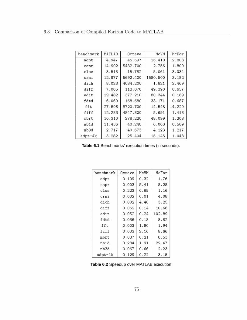
6.3. Comparison of Compiled Fortran Code to MATLAB
benchmark MATLAB Octave McVM McFor
adpt 4.947 45.597 15.410 2.803
capr 14.902 5432.700 2.756 1.800
clos 3.513 15.782 5.061 3.034
crni 12.977 5692.400 1580.500 3.182
dich 8.023 4084.200 1.821 2.469
diff 7.005 113.070 49.390 0.657
edit 19.482 377.210 80.344 0.189
fdtd 6.060 168.680 33.171 0.687
fft 27.596 8720.700 14.548 14.229
fiff 12.283 4847.800 5.691 1.418
mbrt 10.310 278.220 48.099 1.208
nb1d 11.436 40.240 6.003 0.509
nb3d 2.717 40.673 4.123 1.217
adpt-4k 3.282 25.404 15.145 1.043
Table 6.1 Benchmarks’ execution times (in seconds).
benchmark Octave McVM McFor
adpt 0.109 0.32 1.76
capr 0.003 5.41 8.28
clos 0.223 0.69 1.16
crni 0.002 0.01 4.08
dich 0.002 4.40 3.25
diff 0.062 0.14 10.66
edit 0.052 0.24 102.89
fdtd 0.036 0.18 8.82
fft 0.003 1.90 1.94
fiff 0.003 2.16 8.66
mbrt 0.037 0.21 8.53
nb1d 0.284 1.91 22.47
nb3d 0.067 0.66 2.23
adpt-4k 0.129 0.22 3.15
Table 6.2 Speedup over MATLAB execution
75
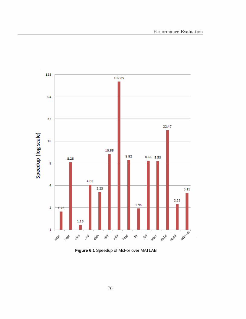
Performance Evaluation
Figure 6.1 Speedup of McFor over MATLAB
76
6.3. Comparison of Compiled Fortran Code to MATLAB
data structures than MATLAB.
Programs that have relatively simple data structures, e.g., one dimensional arrays
or small two-dimensional arrays, and perform mostly double type scalar computations
have a smaller, although still impressive, speedup (1.9 to 4.1). The “fft” benchmark
has a very big one-dimensional array containing 8-million double values, but the
benchmark uses those values sequentially and only performs scalar computations.
Therefore, despite the fact that those computations run about 108 times, the Fortran
code has a limited speedup of 1.94. The benchmark “nb3d” uses six small matrices,
about 75-by-75 each, and it performs simple scalar computations and elementary-wise
matrix-matrix computations on those arrays. Because those small arrays can be easily
cached, the interpretive overheads on accessing them are limited. Thus, the Fortran
code of benchmark “nb3d” has a small speedup of 2.23. The “dich” and “adpt-4k”
benchmarks have similar computations and size of data: “dich” uses a 134-by-134
array and “adpt-4k” uses a 4000-by-6 array. The speedup of compiled Fortran code
on both benchmarks are also similar, 3.25 and 3.15. The “crni” benchmark uses
a larger two-dimensional array (2300-by-2300), and it has computations on partial
arrays, which is more costly in term of accessing data. Therefore, the Fortran code
has a better speedup of 4.08.
For programs performing matrix computations between large matrices, the com-
plied Fortran program has limited speedup over its interpretive execution. This is
because Fortran program uses routines from BLAS and LAPACK libraries to perform
matrix computations, and MATLAB matrix computations are also built on the top
of BLAS and LAPACK and those libraries has been well integrated into MATLAB
runtime environment.
The major computation of the “clos” benchmark is a matrix multiplication, which
consumes over 97% of total execution time. In the generated Fortran code, we use the
dgemm() routine of BLAS library to perform matrix computation. Because in this
benchmark, the multiplication only executes sixty times, the interpretive overhead
for function dispatching is relative small. Therefore, the compiled program has very
limited speedup, 1.16.
We also test the performance of Fortran intrinsic function MATMUL(), which
77
Performance Evaluation
is designed for matrix multiplication. The result shows that for benchmark “clos”,
Fortran code that uses MATMUL() is seven times slower than MATLAB interpretive
execution. We tested MATMUL() on different sizes of arrays, the preliminary results
indicate that MATMUL() performs better than MATLAB only when the sizes of
matrices are smaller than 200-by-200.
The “adpt” benchmark is the program whose performance heavily relies on the
dynamic memory allocations and data copying operations. This benchmark integrates
the function∫−1
6f(x) = 13(x − x2)e−1.5x to a tolerance of 4 × 10⁻¹³. It generates a
result array of size 3270-by-6. This program preallocates the array to the size of
1-by-6 at the beginning, then expands it when the computation requires more space
to store new results.
The inference mechanism cannot predict the final size of the array because it
depends on the tolerance. During the value propagation analysis on array size (as
described in 4.6), the compiler has discovered that several statements whose array
indices are not comparable to the current size of array, and added array bounds
checking code and array expanding code (as described in Section 4.7.2) in front of
those statements to handle the potential array expanding.
The test of the “adpt” benchmark is conducted on total 10 iterations on the func-
tion where the result array is initialized as 1-by-6 then expanded to 3270-by-6. The
execution results show that the Fortran code has about 1.76 speedup, which indicates
that compiled Fortran code performs dynamic reallocations faster than MATLAB in
this case.
The “adpt-4k” is the static version of “adpt”. The “adpt-4k” is tested on the
same code with different conditions, where the array is initialized to the size of 4000-
by-6, thus there is no reallocation occurring in the execution. Comparing to same
interpretive execution in MATLAB, the speedup of “adpt-4k” is 3.1 which is much
higher that “adpt”. The results also show that it has the speedup of 2.6 over Fortran
version of “adpt”. These results show that Fortran has notable overhead when per-
forming dynamic reallocations, and comparing to MATLAB, Fortran is more efficient
for handling large amounts of statically-allocated data.
78
6.4. Comparison of Dynamic Reallocation in Fortran and MATLAB
6.4 Comparison of Dynamic Reallocation in Fortran and
MATLAB
By applying type inference and transformation techniques, McFor is able to infer
array variables’ shapes and declare them statically in most benchmarks. Only one
benchmark “adpt” requires dynamic reallocation code. In order to measure the cost
of reallocations and the potential array expanding strategies, we conducted a set of
experiments on the “adpt” benchmark .
6.4.1 Dynamic Reallocation Tests
In order to get the execution time for different numbers of allocations, we ran the pro-
gram with different preallocation sizes, which are used for initializing the array before
the reallocations. We conducted three sets of tests using three different tolerances.
In the first set of tests, we used a tolerance of 4× 10⁻¹³ and the size of the result
array is 3270-by-6. In the second set of tests, tolerance is 4 × 10⁻¹⁴ and the size of
the result array is 5640-by-6. In the third set of tests, tolerance is 6× 10⁻¹⁵ and the
size of result array is 9490-by-6. During each test, we use different preallocation sizes
until it is over the size of the result array. Figure 6.2, 6.3, and 6.4 shows the speedup
of compiled Fortran code over MATLAB on those three sets of tests respectively.
From the Figure 6.2, 6.3, and 6.4, we observe that the speedup increases as the
number of reallocations decreases, and the increase is greater when the number of
reallocations is smaller than 1500. We also observe that the cost of reallocation also
relates to the size of the array. As the arrays size increases, the speedup decreases. In
the third set of tests (Figure 6.4), where the size of result array is 9490-by-6, compiled
Fortran code even runs slower than MATLAB when number of reallocations is greater
than 3300.
This result shows that Fortran has higher overhead than MATLAB when perform-
ing a large number of reallocations on large arrays.
But when the number of reallocations is small, the compiled Fortran code runs
faster than MATLAB. The “diff” benchmark is another example. The “diff” bench-
79
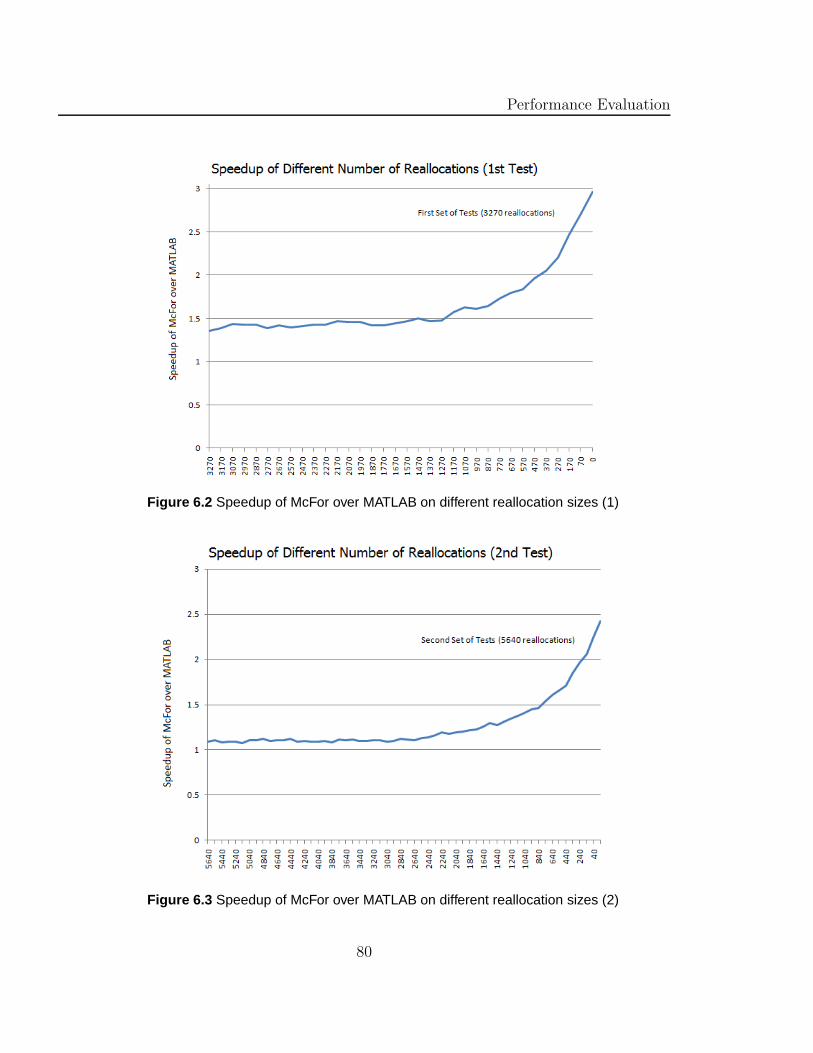
Performance Evaluation
Figure 6.2 Speedup of McFor over MATLAB on different reallocation sizes (1)
Figure 6.3 Speedup of McFor over MATLAB on different reallocation sizes (2)
80
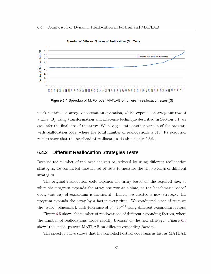
6.4. Comparison of Dynamic Reallocation in Fortran and MATLAB
Figure 6.4 Speedup of McFor over MATLAB on different reallocation sizes (3)
mark contains an array concatenation operation, which expands an array one row at
a time. By using transformation and inference technique described in Section 5.1, we
can infer the final size of the array. We also generate another version of the program
with reallocation code, where the total number of reallocations is 610. Its execution
results show that the overhead of reallocations is about only 2.8%.
6.4.2 Different Reallocation Strategies Tests
Because the number of reallocations can be reduced by using different reallocation
strategies, we conducted another set of tests to measure the effectiveness of different
strategies.
The original reallocation code expands the array based on the required size, so
when the program expands the array one row at a time, as the benchmark “adpt”
does, this way of expanding is inefficient. Hence, we created a new strategy: the
program expands the array by a factor every time. We conducted a set of tests on
the “adpt” benchmark with tolerance of 6× 10⁻¹⁵ using different expanding factors.
Figure 6.5 shows the number of reallocations of different expanding factors, where
the number of reallocations drops rapidly because of the new strategy. Figure 6.6
shows the speedups over MATLAB on different expanding factors.
The speedup curve shows that the compiled Fortran code runs as fast as MATLAB
81
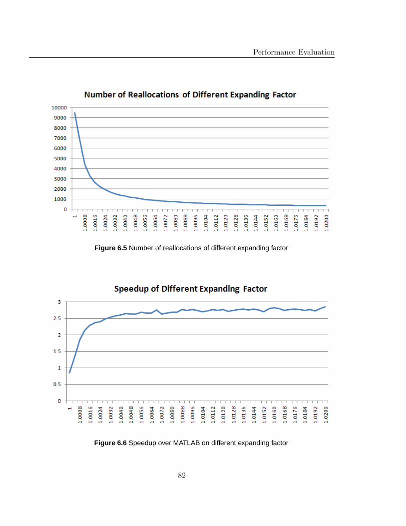
Performance Evaluation
Figure 6.5 Number of reallocations of different expanding factor
Figure 6.6 Speedup over MATLAB on different expanding factor
82
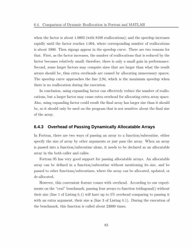
6.4. Comparison of Dynamic Reallocation in Fortran and MATLAB
when the factor is about 1.0003 (with 8100 reallocations); and the speedup increases
rapidly until the factor reaches 1.004, where corresponding number of reallocations
is about 1000. Then zigzags appear in the speedup curve. There are two reasons for
that. First, as the factor increases, the number of reallocations that is reduced by the
factor becomes relatively small; therefore, there is only a small gain in performance.
Second, some larger factors may compute sizes that are larger than what the result
arrays should be, thus extra overheads are caused by allocating unnecessary spaces.
The speedup curve approaches the line 2.94, which is the maximum speedup when
there is no reallocation during the execution.
In conclusion, using expanding factor can effectively reduce the number of reallo-
cations, but a larger factor may cause extra overhead for allocating extra array space.
Also, using expanding factor could result the final array has larger size than it should
be, so it should only be used on the program that is not sensitive about the final size
of the array.
6.4.3 Overhead of Passing Dynamically Allocatable Arrays
In Fortran, there are two ways of passing an array to a function/subroutine, either
specify the size of array by other arguments or just pass the array. When an array
is passed into a function/subroutine alone, it needs to be declared as an allocatable
array in the both caller and callee.
Fortran 95 has very good support for passing allocatable arrays. An allocatable
array can be defined in a function/subroutine without mentioning its size, and be
passed to other functions/subroutines, where the array can be allocated, updated, or
de-allocated.
However, this convenient feature comes with overhead. According to our experi-
ments on the “crni” benchmark, passing four arrays to function tridiagonal() without
their size (line 1 of Listing 6.1) will have up to 5% overhead comparing to passing it
with an extra argument, their size n (line 3 of Listing 6.1). During the execution of
the benchmark, this function is called about 23000 times.
83
Performance Evaluation
1 SUBROUTINE tridiagonal(A, D, C, B, X)
2
3 SUBROUTINE tridiagonal(A, D, C, B, n, X)
Listing 6.1 Passing array with or without its size.
6.5 Summary of Fortran 95 vs. MATLAB
Fortran 95 has less overhead on accessing large amount of data and complex data
structures (e.g., three-dimensional arrays). Fortran 95 has large advantage on smaller
size element-wise vector-vector computations and complex type data computations.
Most basic built-in functions, e.g., sin(), cos(), abs(), exp(), run faster in compiled
Fortran codes than in MATLAB.
Compiled Fortran code is very efficient when performing a small number of reallo-
cations on small arrays. For programs with a large number of reallocations, using an
expanding factor can effectively reduce the reallocation overhead. Therefore, MAT-
LAB programs with dynamic allocations can obtain performance improvement by
translating into Fortran code.
MATLAB performs matrix-matrix computations very efficiently. MATLAB has
efficient loop control structures. In all benchmarks, there are no notable overhead ac-
cumulated by a large number of iterations. MATLAB has improved its performance
on double type scalar computations and accessing one-dimensional array and small
two-dimensional matrices. However, due to its interpretive overheads on type infer-
ence, array bounds checking, and memory accessing, MATLAB programs are still
significantly slower than compiled Fortran codes.
6.6 Comparison of Compiled Fortran Code to Octave
Octave [Eat02] is a MATLAB compatible interpreter, which like McFor, is an open
source project. The experimental results show that for all benchmarks, the com-
piled Fortran codes have better performance than interpretive execution in Octave.
Speedups of some benchmarks are over 1000. Those benchmarks include “capr”,
84
6.7. Comparison of Compiled Fortran Code to McVM
“crni”, “dich”, “edit”, and “fiff”. The major computations of those benchmarks are
scalar computations but run in a loop with a large number of iterations. The results
show that in Octave, the interpretive overhead accumulates heavily over the large
number of iterations.
Comparing to other benchmarks, Octave runs the “clos” benchmark relatively
efficiently. The speedup of compiled Fortran code over Octave is 5.2, the lowest of
all benchmarks. Octave’s numerical libraries also use BLAS to perform the matrix
computation, but the BLAS routines are wrapped into C++ classes. Because the
matrix computation in “clos” consumes over 97% of total execution time, this result
shows that Octave’s numerical libraries have very high overhead for performing the
basic matrix computation.
6.7 Comparison of Compiled Fortran Code to McVM
The McVM virtual machine is a MATLAB just-in-time compiler developed by Maxime
Chevalier-Boisvert of the McLab team [CB09]. It is also a component of the McLab
project, and uses the same MATLAB-to-Natlab translator, Lexer and Parser as Mc-
For does. McVM uses LLVM [LA04] as JIT engine to emit assembly code. We were
able to use an alpha version (0.5) of McVM to get some initial results.
The experimental results shows that except one benchmark, “dich”, compiled
Fortran codes have better performance than McVM.
The speedup of McVM over compiled Fortran code on the “dich” benchmark is
about 1.4. The explanation for this result is that, the benchmark program has been
fully compiled by the McVM JIT compiler and the assembly code generated by LLVM
JIT engine is more efficient than the executable code created by gfortran compiler.
The “dich” benchmark is a loop-based program that mostly performs scalar oper-
ations. The type and shape of two array variables can all be inferred by the compiler.
Its major computations happen inside two nested for-loops, the numbers of iterations
of both loops can be predicted at compile time. Because those scalar computations,
for-loops, and array accesses are fully supported by the LLVM assembly instruction
set, the LLVM JIT engine can generate efficient assembly code for that code segment.
85
Performance Evaluation
Benchmarks that have similar computations also perform well in McVM. Those
benchmarks include “capr”, “fft”, “fiff”, and “nb1d”. McVM out performs MATLAB
on those benchmarks.
Because the LLVM assembly instruction set cannot directly represent complex
data structures (such as three-dimensional arrays and the complex data type) and
matrix computations, McVM performs less efficiently on other benchmarks.
86
Chapter 7
Conclusions and Future Work
7.1 Conclusions
The main goal of this thesis is to apply type inference techniques that have been
developed for array program languages and build an open source MATLAB-to-Fortran
95 compiler to generate efficient Fortran code. Our inference process aims to infer
variables’ type and shape information as much as possible at compile time, so that the
generated code can avoid runtime overhead on type checking and array reallocations.
We developed a type hierarchy and analysis to infer the intrinsic type of all vari-
ables. In order to maximally predict the shape of array variables at compile time, we
developed special transformations to handle array concatenation operations, and a
value propagation analysis to estimate the maximum size of arrays. For the remain-
ing cases, where the size of array cannot be predicted at compile time, we generated
code to dynamically check the size of array and reallocate the array when it is nec-
essary. By using those techniques, only one of twelve benchmarks requires dynamic
reallocation code.
Another goal of our work is to generate programmer-friendly code that is easy to
understand, debug, and reuse. Fortran 95 is the best target language because Fortran
95 has the closest syntax and semantics, which makes translated code closer to the
87
Conclusions and Future Work
original MATLAB program. To keep the program structure, we compiled every user-
defined function independently, and preserved their function declarations in the target
Fortran code. To avoid unnecessary renaming, we did not choose SSA form as our
intermediate representation, but used an extended AST with type conflict functions
that are used to explicitly capture potential type changes in the program.
The performance evaluation results show that the compiled programs perform
better than their MATLAB executions, but the speedups varies, ranging from 1.16
to 102, depending on the characteristics of the program. We also observe that char-
acter operations are executed very slowly in MATLAB, Fortran code handles large
multi-dimensional arrays very efficiently, MATLAB’s built-in function for matrix mul-
tiplication on large arrays is faster than Fortran’s intrinsic function, and a different
reallocation strategy can improve the performance for programs with a larger number
of reallocations.
7.2 Future Work
There are several possible further projects for McFor that can further improve the
performance of generated Fortran code.
1. It would be useful to gather the structural information of matrices and use them
for selecting appropriate Fortran implementations for matrix computations.
The structure of a matrix decides whether the matrix is a square, sparse,
triangular, symmetric, Hermitian, or another type of matrix. It is another im-
portant property the affects the matrix computations. For example, the appro-
priate algorithm for solving a matrix left division operation A\B is dependent on
the structures of matrices A and B. Moreover, some MATLAB built-in functions
are specifically designed for diagonal matrices and sparse matrices. Therefore,
by using the structural information of matrices with their type and shape infor-
mation, the code generator could select more appropriate library routines that
can efficiently perform the computation.
88
7.2. Future Work
2. With many new features introduced by the recent Fortran standards, we believe
that most MATLAB features can be translated into efficient Fortran implemen-
tations.
Fortran has developed from a simple procedural programming language to
a modern programming language. Fortran 2003, the most recent standard, has
extended Fortran to object-oriented and generic programming. Fortran 2003
introduces new features that can be used to implement many MATLAB special
features. For example, Fortran 2003 supports Cray pointers, C-like pointers that
can point to a function or subroutine, which can be used to simulate the function
handles of MATLAB. Fortran 2003 supports “submodules”, which are similar to
the MATLAB’s embedded functions. Fortran 2003 also supports parameterized
derived type and allows allocatable arrays and pointes as components, which
can be used for implementing MATLAB’s cell array and structure.
3. Parallelization
Exploiting parallelism can further improve the performance of the generated
code. After inferring shapes of array variables, many data-dependent analysis
and parallelization optimizations can be added to the compiler. Another pos-
sible approach is to integrate McFor with other Fortran parallel compilers to
generate parallel programs. One way of the integration is to generate the par-
allelization directives, such as OpenMP Fortran API directives, for a target
parallel compiler by utilizing the information gathered by the inference process.
Another way is to provide direct information using internal data to parallel
compilers to facilitate the work of their parallel optimizers.
4. Improving Readability
There are several improvements can be done to elevate the readability of
the target code.
(a) Remove temporary variables.
There are some temporary variables generated by the simplification
transformation and type inference process that could not be removed by
89
Conclusions and Future Work
the current aggregation transformation. The aggregation transformation
is designed to reverse the simplification transformation based on the flow
analysis. However, some temporary variables cannot be merged back to
their original places because of restrictions of Fortran language. For ex-
ample, the array construction expression (e.g. data=[a,b]), requires all
elements (a,b) to have the same type. The following is a Fortran code seg-
ment with temporary variables. If merging two temporary variables to the
third statement, the result statement, output=[2.2, 1], becomes illegal in
Fortran.
DOUBLE PRECISION:: tmpvar3, tmpvar4;
tmpvar3=2.2; tmpvar4=1; output=[tmpvar3, tmpvar4];
It is possible to enhance the aggregation transformation to solve those
special cases.
(b) Restore the original names of renamed variables
Some variables were renamed for special purposes during the process of
building the symbol table, and their original names could be restored back
afterwards. For instance, for simplifying the value-propagation process,
some loop variables are renamed in order to keep a unique definition. Those
renamings could be reversed after type inference and transformation phase.
(c) Restore and add comments
Comments in the MATLAB programs are reserved during the lexing
and parsing. However, there are a number of cases where a comment
cannot be restored to the exactly location as in the original code.
Some Fortran code segments that are generated by some transforma-
tions become very different from the original MATLAB statements. List-
ing the original MATLAB statements as comments beside the transformed
code would be helpful for programmers to understand the new code.
90
Appendix A
Supported MATLAB Features
The McFor compiler supports a subset of MATLAB features that are commonly
used for scientific computation. The following is a list of all MATLAB features the
supported by McFor compiler.
Program control statements :
• Conditional control statements: if-elseif-else-end, switch-case-otherwise-
end.
• Loop control statements: for, while, continue, break.
• Program Termination: return.
Operators :
• Arithmetic Operators: “+”, “-”, “*”, “/”, “\”, “^”, “.*”, “./”, “.\”, “.^”,
“.’”, “’”, “:”,
• Relational Operators: “<”, “<=”, “>”, “>=”, “==”, “ =”,
• Logical Operators: “&”, “|”, “ ”, “xor”, “&&”, “||”,
Data Type: logical, integer, single, double, complex, character, string.
Matrix Construction: e.g., row=[E1 E2 ...Em]; A=[row1; row2; ...; rown]. (dis-
cussed in Section 5.1)
91
Supported MATLAB Features
Matrix Concatenation: e.g., C=[A,B]; C=[A;B]. (discussed in Section 5.1)
Matrix Indexing :
• Linear Indexing: discussed in Section 5.2
• Using an Array as an Index: including using logical array as index: dis-
cussed in Section 5.3
• Accessing Multiple Elements
– Consecutive Elements: A(1:6, 2); A(1:6, 2:3).
– Nonconsecutive Elements: B(1:3:16)=-10
– Specifying All Elements of a Row or Column: A(:), A(:,2), A(2,:)
Empty Matrices : e.g., A(:,3)=[]; A(3:4,:)=[];
Resizing Matrices :
Three situations that a variable’s shape can dynamically change : when a new
value with different shape is assigned to it, when new elements are added to
a location outside the bounds of the variable, or when rows and columns are
deleted from the variable. They are discussed in Section 4.4.2 and Section 4.1.3
92
Bibliography
[ABB+99] E. Anderson, Z. Bai, C. Bischof, L. S. Blackford, J. Demmel, Jack J.
Dongarra, J. Du Croz, S. Hammarling, A. Greenbaum, A. McKenney, and
D. Sorensen. LAPACK Users’ guide (third ed.). Society for Industrial and
Applied Mathematics, Philadelphia, PA, USA, 1999.
[AK87] Randy Allen and Ken Kennedy. Automatic translation of Fortran pro-
grams to vector form. ACM Trans. Program. Lang. Syst., 9(4):491–542,
1987.
[AK02] Randy Allen and Ken Kennedy. Optimizing Compilers for Modern Ar-
chitectures: A Dependence-Based Approach. Morgan Kaufmann, 2002.
[AP02] George Almasi and David Padua. MaJIC: compiling MATLAB for speed
and responsiveness. In PLDI ’02: Proceedings of the ACM SIGPLAN
2002 Conference on Programming language design and implementation,
Berlin, Germany, 2002, pages 294–303. ACM, New York, NY, USA.
[BLA07] Neil Birkbeck, Jonathan Levesque, and Jose Nelson Amaral. A Dimension
Abstraction Approach to Vectorization in Matlab. In CGO ’07: Proceed-
ings of the International Symposium on Code Generation and Optimiza-
tion, 2007, pages 115–130. IEEE Computer Society, Washington, DC,
USA.
93
Bibliography
[Bud83] Timothy A. Budd. An APL compiler for the UNIX timesharing system.
In APL ’83: Proceedings of the international conference on APL, Wash-
ington, D.C., United States, 1983, pages 205–209. ACM, New York, NY,
USA.
[Cas09] Andrew Casey. The Metalexer Lexer Specification Language. Master’s
thesis, School of Computer Science, McGill University, Montreal, Canada,
2009.
[CB09] Maxime Chevalier-Boisvert. McVM: An Optimizing Virtual Machine For
The MATLAB Programming Language. Master’s thesis, School of Com-
puter Science, McGill University, Montreal, Canada, 2009.
[CBHV10] Maxime Chevalier-Boisvert, Laurie Hendren, and Clark Verbrugge. Op-
timizing MATLAB through Just-In-Time Specialization. In CC 2010:
International Conference on Compiler Construction, 2010.
[CDD+95] J. Choi, J. Demmel, I. Dhillon, J. Dongarra, S. Ostrouchov, A. Petitet,
K. Staney, D. Walker, and R. C. Whaley. LAPACK Working Note 95:
ScaLAPACK: A Portable Linear Algebra Library for Distributed Memory
Computers – Design Issues and Performance. Technical report, Knoxville,
TN, USA, 1995.
[Chi86] W-M Ching. Program analysis and code generation in an APL/370 com-
piler. IBM J. Res. Dev., 30(6):594–602, 1986.
[Eat02] John W. Eaton. GNU Octave Manual. Network Theory Limited, 2002.
[EH07] Torbjorn Ekman and Gorel Hedin. The JastAdd system — modular
extensible compiler construction. Sci. Comput. Program., 69(1-3):14–26,
2007.
[Eng96] Dawson R. Engler. VCODE: a retargetable, extensible, very fast dynamic
code generation system. SIGPLAN Not., 31(5):160–170, 1996.
94
Bibliography
[HNK+00] Malay Haldar, Anshuman Nayak, Abhay Kanhere, Pramod Joisha, Na-
garaj Shenoy, Alok Choudhary, and Prithviraj Banerjee. Match Virtual
Machine: An Adaptive Runtime System to Execute MATLAB in Paral-
lel. In ICPP ’00: Proceedings of the Proceedings of the 2000 International
Conference on Parallel Processing, 2000, page 145. IEEE Computer Soci-
ety, Washington, DC, USA.
[Inc08] MathWorks Inc. MATLAB Documentation, 2008.
<http://www.mathworks.com/> .
[Inc09] Free Software Foundation Inc. GCC, the GNU Compiler Collection, 2009.
<http://gcc.gnu.org/> .
[INR09] INRIA. Scilab, 2009.
<http://www.scilab.org/platform/> .
[JB01] Pramod G. Joisha and Prithviraj Banerjee. Correctly detecting intrinsic
type errors in typeless languages such as MATLAB. In APL ’01: Pro-
ceedings of the 2001 conference on APL, New Haven, Connecticut, 2001,
pages 7–21. ACM, New York, NY, USA.
[JB02] Pramod G. Joisha and Prithviraj Banerjee. MAGICA: A Software Tool
for Inferring Types in MATLAB. 2002.
[JB03] Pramod G. Joisha and Prithviraj Banerjee. Static array storage opti-
mization in MATLAB. In PLDI ’03: Proceedings of the ACM SIGPLAN
2003 conference on Programming language design and implementation,
San Diego, California, USA, 2003, pages 258–268. ACM, New York, NY,
USA.
[Joi03a] Pramod G. Joisha. a MATLAB-to-C translator, 2003.
<http://www.ece.northwestern.edu/cpdc/pjoisha/mat2c/> .
95
Bibliography
[Joi03b] Pramod G. Joisha. A type inference system for MATLAB with applica-
tions to code optimization. PhD thesis, Evanston, IL, USA, 2003. Adviser-
Banerjee, Prithviraj.
[KU80] Marc A. Kaplan and Jeffrey D. Ullman. A Scheme for the Automatic
Inference of Variable Types. J. ACM, 27(1):128–145, 1980.
[LA04] Chris Lattner and Vikram Adve. LLVM: A Compilation Framework for
Lifelong Program Analysis & Transformation. In CGO ’04: Proceedings of
the international symposium on Code generation and optimization, Palo
Alto, California, 2004, page 75. IEEE Computer Society, Washington,
DC, USA.
[Ltd99] MathTools Ltd. MATCOM compiler, 1999.
<http://www.mathtools.com/> .
[MC07] D. Mcfarlin and A. Chauhan. Library Function Selection in Compiling
Octave. In Parallel and Distributed Processing Symposium, 2007. IPDPS
2007. IEEE International, 2007, pages 1–8.
[MHK+00] Anshuman Nayak Malay, Malay Haldar, Abhay Kanhere, Pramod Joisha,
Nagaraj Shenoy, Alok Choudhary, and Prithviraj Banerjee. A Library
based compiler to execute MATLAB Programs on a Heterogeneous Plat-
form, 2000.
[MP99] Vijay Menon and Keshav Pingali. High-level semantic optimization of
numerical codes. In ICS ’99: Proceedings of the 13th international con-
ference on Supercomputing, Rhodes, Greece, 1999, pages 434–443. ACM,
New York, NY, USA.
[MT97] Vijay Menon and Anne E. Trefethen. MultiMATLAB: Integrating MAT-
LAB with High-Performance Parallel Computing. In In Proceedings of
Supercomputing ’97, 1997, pages 1–18.
96
Bibliography
[QMSZ98] Michael J. Quinn, Alexey Malishevsky, Nagajagadeswar Seelam, and Yan
Zhao. Preliminary Results from a Parallel MATLAB Compiler. In Proc.
Int. Parallel Processing Symp. (IPPS, 1998, pages 81–87. IEEE CS Press.
[RHB96] Shankar Ramaswamy, Eugene W. Hodges, IV, and Prithviraj Banerjee.
Compiling MATLAB Programs to ScaLAPACK: Exploiting Task and
Data Parallelism. In IPPS ’96: Proceedings of the 10th International
Parallel Processing Symposium, 1996, pages 613–619. IEEE Computer
Society, Washington, DC, USA.
[RP96] Luiz De Rose and David Padua. A MATLAB to Fortran 90 translator and
its effectiveness. In ICS ’96: Proceedings of the 10th international con-
ference on Supercomputing, Philadelphia, Pennsylvania, United States,
1996, pages 309–316. ACM, New York, NY, USA.
[RP99] Luiz De Rose and David Padua. Techniques for the translation of MAT-
LAB programs into Fortran 90. ACM Trans. Program. Lang. Syst.,
21(2):286–323, 1999.
[Sch75] J. T. Schwartz. Automatic data structure choice in a language of very
high level. Commun. ACM, 18(12):722–728, 1975.
[TP95] Peng Tu and David Padua. Gated SSA-based demand-driven symbolic
analysis for parallelizing compilers. In ICS ’95: Proceedings of the 9th in-
ternational conference on Supercomputing, Barcelona, Spain, 1995, pages
414–423. ACM, New York, NY, USA.
[vB05] Remko van Beusekom. A Vectorizer for Octave. Master’s thesis, Utrecht
University, Utrecht, The Netherlands, February 2005. INF/SRC-04-53.
[WPF07] William Vetterling William Press, Saul Teukolsky and Brian Flannery.
Numerical Recipes: the art of scientific computing. Cambridge University
Press, 2007.
97
Bibliography
[WS81] Zvi Weiss and Harry J. Saal. Compile time syntax analysis of APL pro-
grams. In APL ’81: Proceedings of the international conference on APL,
San Francisco, California, United States, 1981, pages 313–320. ACM, New
York, NY, USA.
98