mclust 5: clustering, classiﬁcation and density ... · contributed research articles 289 mclust...

CONTRIBUTED RESEARCH ARTICLES 289

mclust 5: Clustering, Classification andDensity Estimation Using Gaussian FiniteMixture Modelsby Luca Scrucca, Michael Fop, T. Brendan Murphy and Adrian E. Raftery

Abstract Finite mixture models are being used increasingly to model a wide variety of randomphenomena for clustering, classification and density estimation. mclust is a powerful and popularpackage which allows modelling of data as a Gaussian finite mixture with different covariancestructures and different numbers of mixture components, for a variety of purposes of analysis. Recently,version 5 of the package has been made available on CRAN. This updated version adds new covariancestructures, dimension reduction capabilities for visualisation, model selection criteria, initialisationstrategies for the EM algorithm, and bootstrap-based inference, making it a full-featured R packagefor data analysis via finite mixture modelling.

Introduction

mclust (Fraley et al., 2016) is a popular R package for model-based clustering, classification, anddensity estimation based on finite Gaussian mixture modelling. An integrated approach to finitemixture models is provided, with functions that combine model-based hierarchical clustering, EMfor mixture estimation and several tools for model selection. Thus mclust provides a comprehensivestrategy for clustering, density estimation and discriminant analysis. A variety of covariance structuresobtained through eigenvalue decomposition are available. Functions for performing single E andM steps and for simulating data for each available model are also included. Additional ways ofdisplaying and visualising fitted models along with clustering, classification, and density estimationresults are also provided. It has been used in a broad range of contexts including geochemistry (Templet al., 2008; Ellefsen et al., 2014), chemometrics (Fraley and Raftery, 2006a, 2007b), DNA sequenceanalysis (Verbist et al., 2015), gene expression data (Yeung et al., 2001; Li et al., 2005; Fraley and Raftery,2006b), hydrology (Kim et al., 2014), wind energy (Kazor and Hering, 2015), industrial engineering(Campbell et al., 1999), epidemiology (Flynt and Daepp, 2015), food science (Kozak and Scaman,2008), clinical psychology (Suveg et al., 2014), political science (Ahlquist and Breunig, 2012; Jang andHitchcock, 2012), and anthropology (Konigsberg et al., 2009).

One measure of the popularity of mclust is provided by the download logs of the RStudio(http://www.rstudio.com) CRAN mirror (available at http://cran-logs.rstudio.com). The cran-logs package (Csardi, 2015) makes it easy to download such logs and graph the number of downloadsover time. We used cranlogs to query the RStudio download database over the past three years. Inaddition to mclust, other R packages which handle Gaussian finite mixture modelling as part of theircapabilities have been included in the comparison: Rmixmod (Lebret et al., 2015), mixture (Browneet al., 2015), EMCluster (Chen and Maitra, 2015), mixtools (Benaglia et al., 2009), and bgmm (Bieceket al., 2012). We also included flexmix (Leisch, 2004; Grün and Leisch, 2007, 2008) which provides ageneral framework for finite mixtures of regression models using the EM algorithm, since it can beadapted to perform Gaussian model-based clustering using a limited set of models (only the diagonaland unconstrained covariance matrix models). Table 1 summarises the functionalities of the selectedpackages.

Package Version Clustering Classification Densityestimation

Non-Gaussiancomponents

mclust 5.2 3 3 3 7Rmixmod 2.0.3 3 3 7 3mixture 1.4 3 3 7 7EMCluster 0.2-5 3 3 7 7mixtools 1.0.4 3 7 3 3bgmm 1.7 3 3 7 7flexmix 2.3-13 3 7 7 3

Table 1: Capabilities of the selected packages dealing with finite mixture models.

Figure 1 shows the trend in weekly downloads from the RStudio CRAN mirror for the selected

The R Journal Vol. 8/1, Aug. 2016 ISSN 2073-4859

http://CRAN.R-project.org/package=mclust

http://www.rstudio.com

http://cran-logs.rstudio.com

http://CRAN.R-project.org/package=cranlogs

http://CRAN.R-project.org/package=cranlogs

http://CRAN.R-project.org/package=Rmixmod

http://CRAN.R-project.org/package=mixture

http://CRAN.R-project.org/package=EMCluster

http://CRAN.R-project.org/package=mixtools

http://CRAN.R-project.org/package=bgmm

http://CRAN.R-project.org/package=flexmix


packages. The popularity of mclust has been increasing steadily over time with a first high peakaround mid April 2015, probably due to the release of R version 3.2 and, shortly after, the release ofversion 5 of mclust. Then, successive peaks occurred in conjunction with the release of package’supdates. Based on these logs, mclust is the most downloaded package dealing with Gaussian mixturemodels, followed by flexmix which, as mentioned, is a more general package for fitting mixturemodels but with limited clustering capabilities.

4.1 4.2 4.3 4.4 5.0 5.1 5.2

0

2000

4000

6000

2013 2014 2015 2016

Num

ber

of w

eekl

y do

wnl

oads

mclust Rmixmod mixture EMCluster mixtools bgmm flexmix

Figure 1: Number of weekly downloads from the RStudio CRAN mirror over time for some R packagesdealing with Gaussian finite mixture modelling.

Another aspect that can be considered as a proxy for the popularity of a package is the mutualdependencies structure between R packages1. This can be represented as a graph with packages at thevertices and dependencies (either “Depends”, “Imports”, “LinkingTo”, “Suggests” or “Enhances”) asdirected edges, and analysed through the PageRank algorithm used by the Google search engine (Brinand Page, 1998). For the packages considered previously, we used the page.rank function availablein the igraph package (Csardi and Nepusz, 2006) and we obtained the ranking reported in Table 2,which approximately reproduces the results discussed above. Note that mclust is among the top 100packages on CRAN by this ranking. Finally, its popularity is also indicated by the 55 other CRANpackages listed as reverse dependencies, either “Depends”, “Imports” or “Suggests”.

mclust Rmixmod mixture EMCluster mixtools bgmm flexmix

75 2300 2319 2143 1698 3736 270

Table 2: Ranking obtained with the PageRank algorithm for some R packages dealing with Gaussianfinite mixture modelling. At the time of writing there are 8663 packages on CRAN.

Earlier versions of the package have been described in Fraley and Raftery (1999), Fraley andRaftery (2003), and Fraley et al. (2012). In this paper we discuss some of the new functionalitiesavailable in mclust version ≥ 5. In particular we describe the newly available models, dimensionreduction for visualisation, bootstrap-based inference, implementation of different model selectioncriteria and initialisation strategies for the EM algorithm.

The reader should first install the latest version of the package from CRAN with

> install.packages("mclust")

1See http://piccolboni.info/2012/05/essential-r-packages.html.


http://CRAN.R-project.org/package=igraph

http://piccolboni.info/2012/05/essential-r-packages.html


Then the package is loaded into an R session using the command

> library(mclust)__ ___________ __ _____________

/ |/ / ____/ / / / / / ___/_ __// /|_/ / / / / / / / /\__ \ / /

/ / / / /___/ /___/ /_/ /___/ // //_/ /_/\____/_____/\____//____//_/ version 5.2Type 'citation("mclust")' for citing this R package in publications.

All the datasets used in the examples are available in mclust or in other R packages, such as gclus(Hurley, 2012), rrcov (Todorov and Filzmoser, 2009) and tourr (Wickham et al., 2011), and can beinstalled from CRAN using the above procedure, except where noted differently.

Gaussian finite mixture modelling

Let x = {x1, x2, . . . , xi, . . . , xn} be a sample of n independent identically distributed observations. Thedistribution of every observation is specified by a probability density function through a finite mixturemodel of G components, which takes the following form

f (xi; Ψ) =G

∑k=1

πk fk(xi; θk), (1)

where Ψ = {π1, . . . , πG−1, θ1, . . . , θG} are the parameters of the mixture model, fk(xi; θk) is the kthcomponent density for observation xi with parameter vector θk, (π1, . . . , πG−1) are the mixing weightsor probabilities (such that πk > 0, ∑G

k=1 πk = 1), and G is the number of mixture components.

Assuming that G is fixed, the mixture model parameters Ψ are usually unknown and must beestimated. The log-likelihood function corresponding to equation (1) is given by `(Ψ; x1, . . . , xn) =∑n

i=1 log( f (xi; Ψ)). Direct maximisation of the log-likelihood function is complicated, so the maximumlikelihood estimator (MLE) of a finite mixture model is usually obtained via the EM algorithm(Dempster et al., 1977; McLachlan and Peel, 2000).

In the model-based approach to clustering, each component of a finite mixture density is usuallyassociated with a group or cluster. Most applications assume that all component densities arise fromthe same parametric distribution family, although this need not be the case in general. A popularmodel is the Gaussian mixture model (GMM), which assumes a (multivariate) Gaussian distributionfor each component, i.e. fk(x; θk) ∼ N(µk, Σk). Thus, clusters are ellipsoidal, centered at the meanvector µk, and with other geometric features, such as volume, shape and orientation, determined bythe covariance matrix Σk. Parsimonious parameterisations of the covariances matrices can be obtainedby means of an eigen-decomposition of the form Σk = λkDk AkD>k , where λk is a scalar controllingthe volume of the ellipsoid, Ak is a diagonal matrix specifying the shape of the density contours withdet(Ak) = 1, and Dk is an orthogonal matrix which determines the orientation of the correspondingellipsoid (Banfield and Raftery, 1993; Celeux and Govaert, 1995). In one dimension, there are just twomodels: E for equal variance and V for varying variance. In the multivariate setting, the volume, shape,and orientation of the covariances can be constrained to be equal or variable across groups. Thus,14 possible models with different geometric characteristics can be specified. Table 3 reports all suchmodels with the corresponding distribution structure type, volume, shape, orientation, and associatedmodel names. In Figure 2 the geometric characteristics are shown graphically.

Starting with version 5.0 of mclust, four additional models have been included: EVV, VEE, EVE,VVE. Models EVV and VEE are estimated using the methods described in Celeux and Govaert (1995),and the estimation of models EVE and VVE is carried out using the approach discussed by Browneand McNicholas (2014). In the models VEE, EVE and VVE it is assumed that the mixture componentsshare the same orientation matrix. This assumption allows for a parsimonious characterisation of theclusters, while still retaining flexibility in defining volume and shape.

Model-based clustering

To illustrate the new modelling capabilities of mclust for model-based clustering consider the winedataset contained in the gclus R package. This dataset provides 13 measurements obtained from achemical analysis of 178 wines grown in the same region in Italy but derived from three differentcultivars (Barolo, Grignolino, Barbera).


http://CRAN.R-project.org/package=gclus

http://CRAN.R-project.org/package=rrcov

http://CRAN.R-project.org/package=tourr


Model Σk Distribution Volume Shape Orientation

EII λI Spherical Equal Equal —VII λk I Spherical Variable Equal —EEI λA Diagonal Equal Equal Coordinate axesVEI λk A Diagonal Variable Equal Coordinate axesEVI λAk Diagonal Equal Variable Coordinate axesVVI λk Ak Diagonal Variable Variable Coordinate axesEEE λDAD> Ellipsoidal Equal Equal EqualEVE λDAkD> Ellipsoidal Equal Variable EqualVEE λkDAD> Ellipsoidal Variable Equal EqualVVE λkDAkD> Ellipsoidal Variable Variable EqualEEV λDk AD>k Ellipsoidal Equal Equal VariableVEV λkDk AD>k Ellipsoidal Variable Equal VariableEVV λDk AkD>k Ellipsoidal Equal Variable VariableVVV λkDk AkD>k Ellipsoidal Variable Variable Variable

Table 3: Parameterisations of the within-group covariance matrix Σk for multidimensional dataavailable in the mclust package, and the corresponding geometric characteristics.

EII VII EEI VEI EVI

VVI EEE EVE VEE EEV

VEV EVV VVE VVV

Figure 2: Ellipses of isodensity for each of the 14 Gaussian models obtained by eigen-decompositionin case of three groups in two dimensions.

> data(wine, package = "gclus")> Class <- factor(wine$Class, levels = 1:3,

labels = c("Barolo", "Grignolino", "Barbera"))> X <- data.matrix(wine[,-1])> mod <- Mclust(X)> summary(mod$BIC)Best BIC values:

EVE,3 VVE,3 VVE,6BIC -6873.257 -6896.83693 -6906.37460BIC diff 0.000 -23.57947 -33.11714> plot(mod, what = "BIC", ylim = range(mod$BIC[,-(1:2)], na.rm = TRUE),

legendArgs = list(x = "bottomleft"))

In the above Mclust() function call, only the data matrix is provided, and the number of mixing



−95

00−

9000

−85

00−

8000

−75

00−

7000

Number of components

BIC

●

●

●● ● ● ●

● ●

●

●

●●

●●

●●

●

●

●

●

● ● ●

●

●

●

●

●

● ●●

●

●

●

●

1 2 3 4 5 6 7 8 9

●

●

●

●

EIIVIIEEIVEIEVIVVIEEE

EVEVEEVVEEEVVEVEVVVVV

Figure 3: BIC plot for models fitted to the wine data.

components and the covariance parameterisation are selected using the Bayesian Information Criterion(BIC). A summary showing the top-three models and a plot of the BIC traces (see Figure 3) for all themodels considered is then obtained. In the last plot we adjusted the range of the y-axis so to removethose models with lower BIC values. There is a clear indication of a three-component mixture withcovariances having different shapes but the same volume and orientation (EVE). Note that all the topthree models are among the models added to the latest major release of mclust.

A summary of the selected model is obtained as:

> summary(mod)----------------------------------------------------Gaussian finite mixture model fitted by EM algorithm----------------------------------------------------

Mclust EVE (ellipsoidal, equal volume and orientation) model with 3 components:

log.likelihood n df BIC ICL-3032.45 178 156 -6873.257 -6873.549

Clustering table:1 2 363 51 64

The fitted model provides an accurate recovery of the true classes:

> table(Class, mod$classification)Class 1 2 3Barolo 59 0 0Grignolino 4 3 64Barbera 0 48 0

> adjustedRandIndex(Class, mod$classification)[1] 0.8803998

The latter index is the adjusted Rand index (ARI; Hubert and Arabie, 1985), which can be used forevaluating a clustering solution. The ARI is a measure of agreement between two partitions, oneestimated by a statistical procedure independent of the labelling of the groups, and one being the trueclassification. It has zero expected value in the case of a random partition, and it is bounded above by1, with higher values representing better partition accuracy.

To visualise the clustering structure and the geometric characteristics induced by an estimatedGaussian finite mixture model we may project the data onto a suitable dimension reduction subspace.The function MclustDR() implements the methodology introduced in Scrucca (2010). The estimateddirections which span the reduced subspace are defined as a set of linear combinations of the originalfeatures, ordered by importance as quantified by the associated eigenvalues. By default, information onthe dimension reduction subspace is provided by both the variation on cluster means and, depending



on the estimated mixture model, on the variation on cluster covariances. This methodology hasbeen extended to supervised classification by Scrucca (2014). Furthermore, a tuning parameter hasbeen included which enables the recovery of most of the separating directions, i.e. those that showmaximal separation among groups. Other dimension reduction techniques for finding the directions ofoptimum separation have been discussed in detail by Hennig (2004) and implemented in the packagefpc (Hennig, 2015).

Applying MclustDR to the wine data example, such directions are obtained as follows:

> drmod <- MclustDR(mod, lambda = 1)> summary(drmod)-----------------------------------------------------------------Dimension reduction for model-based clustering and classification-----------------------------------------------------------------

Mixture model type: Mclust (EVE, 3)

Clusters n1 632 513 64

Estimated basis vectors:Dir1 Dir2

Alcohol 0.11701058 0.2637302Malic -0.02814821 0.0489447Ash -0.18258917 0.5390056Alcalinity -0.02969793 -0.0309028Magnesium 0.00575692 0.0122642Phenols -0.18497201 -0.0016806Flavanoids 0.45479873 -0.2948947Nonflavanoid 0.59278569 -0.5777586Proanthocyanins 0.05347167 0.0508966Intensity -0.08328239 0.0332611Hue 0.42950365 -0.4588969OD280 0.40563746 -0.0369229Proline 0.00075867 0.0010457

Dir1 Dir2Eigenvalues 1.5794 1.332Cum. % 54.2499 100.000

By setting the optional tuning parameter lambda = 1, instead of the default value 0.5, only theinformation on cluster means is used for estimating the directions. In this case, the dimension ofthe subspace is d = min(p, G− 1), where p is the number of variables and G the number of mixturecomponents or clusters. In the data example, there are p = 13 features and G = 3 clusters, so thedimension of the reduced subspace is d = 2. As a result, the projected data show the maximalseparation among clusters, as shown in Figure 4a, which is obtained with

> plot(drmod, what = "contour")

On the same subspace we can also plot the uncertainty boundaries corresponding to the MAPclassification:

> plot(drmod, what = "boundaries", ngrid = 200)

and then add a circle around the misclassified observations

> miscl <- classError(Class, mod$classification)$misclassified> points(drmod$dir[miscl,], pch = 1, cex = 2)

Model selection

A central question in finite mixture modelling is how many components should be included in themixture. In GMMs we need also to decide which covariance parameterisation to adopt. Both questionscan be addressed by information criteria, such as the BIC (Schwartz, 1978; Fraley and Raftery, 1998)


http://CRAN.R-project.org/package=fpc


−1.5 −1.0 −0.5 0.0 0.5 1.0 1.5

−1.

5−

1.0

−0.

50.

00.

51.

0

Dir1

Dir2

0.5

1

1.5

0.5

1

1.5

0.5

1

1.5

●

●

●

●

●

●●

●

●

●

●

●

●

●

●

●

●

●

●

●

●

● ●

●

●

●

●●

●

●●

●

●

●

●

●

●

●

●

●

●●

●

●●

●

●

●

●●

●

●●

●

●● ●

●

●

●

●●

●

(a)

−1.5 −1.0 −0.5 0.0 0.5 1.0 1.5

−1.

5−

1.0

−0.

50.

00.

51.

0

Dir1

Dir2

●

●

●

●

●

●●

●

●

●

●

●

●

●

●

●

●

●

●

●

●

● ●

●

●

●

●●

●

●●

●

●

●

●

●

●

●

●

●

●●

●

●●

●

●

●

●●

●

●●

●

●● ●

●

●

●

●●

●

● ●● ●●

●●

(b)

Figure 4: Contour plot of estimated mixture densities (a) and uncertainty boundaries (b) on theprojection subspace estimated with MclustDR for the wine dataset.

or the integrated complete-data likelihood criterion (ICL; Biernacki et al., 2000). The selection of theorder of the mixture, i.e. the number of mixture components or clusters, can be also performed byformal hypothesis testing; for a recent review see McLachlan and Rathnayake (2014).

Information criteria are based on penalised forms of the log-likelihood. As the likelihood increaseswith the addition of more components, a penalty term for the number of estimated parameters issubtracted from the log-likelihood. The BIC is a popular choice in the context of GMMs, and takes theform

BICM,G = 2`M,G(x|Ψ)− ν log(n),

where `M,G(x|Ψ) is the log-likelihood at the MLE Ψ for modelM with G components, n is the samplesize, and ν is the number of estimated parameters. The pair {M, G} which maximises BICM,G isselected. Given some necessary regularity conditions, BIC is derived as an approximation to themodel evidence using the Laplace method. Although these conditions do not hold for mixture modelsin general (Aitkin and Rubin, 1985), some consistency results apply (Roeder and Wasserman, 1997;Keribin, 2000) and the criterion has been shown to perform well in applications (Fraley and Raftery,1998).

In the mclust package, BIC is used by default for model selection. The function mclustBIC()allows the user to obtain a matrix of BIC values for all the available models and number of componentsup to 9 (by default).

For example, consider the diabetes dataset which contains measurements on 145 non-obese adultsubjects. Recorded variables are glucose, the area under plasma glucose curve after a three hour oralglucose tolerance test (OGTT), insulin, the area under plasma insulin curve after a three hour OGTT,and sspg, the steady state plasma glucose level. The patients are classified clinically into three groups.

> data(diabetes)> X <- diabetes[,2:4]> Class <- diabetes$class> table(Class)Chemical Normal Overt

36 76 33

The data can be shown graphically (see Figure 5) as follows:

> clp <- clPairs(X, Class, lower.panel = NULL)> clPairsLegend(0.1, 0.3, class = clp$class, col = clp$col, pch = clp$pch)

The following function call can be used to compute the BIC for all the covariance structures andup to 9 components:

> BIC <- mclustBIC(X)> BICBayesian Information Criterion (BIC):

EII VII EEI VEI EVI VVI EEE EVE1 -5863.923 -5863.923 -5530.129 -5530.129 -5530.129 -5530.129 -5136.446 -5136.4462 -5449.518 -5327.719 -5169.399 -5019.350 -5015.884 -4988.322 -5010.994 -4875.633



100 200 300

100

200

300

glucose

0 500 1000 1500

●●●

●●●●●●

●●●

●● ●

●●● ●●●●●●●

●●

●● ●●●

●

●

●●

0 200 400 600

100

200

300

●●●

●● ●●●

●●●

●●

●●● ●●●

●●● ●

●●

●●

●● ●● ●

●

●

●●

insulin

050

010

0015

00

●●●

●● ●●●●

●●●

●●●

● ●●

●

● ●●●●●

●●

●

●

●●

●●

●

●

●

0 200 400 600

020

040

060

0

sspg● Chemical

Normal

Overt

Figure 5: Pairwise scatterplots for the diabetes data with points marked according to classification.

3 -5412.588 -5206.399 -4998.446 -4899.759 -5000.661 -4827.818 -4976.853 -4858.8514 -5236.008 -5208.512 -4937.627 -4835.856 -4865.767 -4813.002 -4865.864 -4793.2615 -5181.608 -5202.555 -4915.486 -4841.773 -4838.587 -4833.589 -4882.812 NA6 -5162.164 -5135.069 -4885.752 NA -4848.623 -4810.558 -4835.226 NA7 -5128.736 -5129.460 -4857.097 NA -4849.023 NA -4805.518 NA8 -5135.787 -5135.053 -4858.904 NA -4873.450 NA -4820.155 NA9 -5150.374 -5112.616 -4878.786 NA -4865.166 NA -4840.039 NA

VEE VVE EEV VEV EVV VVV1 -5136.446 -5136.446 -5136.446 -5136.446 -5136.446 -5136.4462 -4920.301 -4877.086 -4918.500 -4834.727 -4823.779 -4825.0273 -4851.667 -4775.537 -4917.567 -4809.225 -4817.884 -4760.0914 -4840.034 -4794.892 -4887.406 -4823.882 -4828.796 -4802.4205 NA NA -4908.030 -4842.077 NA NA6 NA NA -4844.584 -4826.457 NA NA7 NA NA -4910.155 -4852.182 NA NA8 NA NA -4858.974 -4870.633 NA NA9 NA NA -4930.535 -4887.206 NA NA

Top 3 models based on the BIC criterion:VVV,3 VVE,3 EVE,4

-4760.091 -4775.537 -4793.261

In the results reported above, the NA values mean that a particular model cannot be estimated. Thishappens in practice due to singularity in the covariance matrix estimate and can be avoided usingthe Bayesian regularisation proposed in Fraley and Raftery (2007a) and implemented in mclust asdescribed in Fraley et al. (2012). Optional arguments allow finetuning, such as G for the number ofcomponents, and modelNames for specifying the model covariances parameterisations (see Table 3 andhelp(mclustModelNames) for a description of available model names). Another optional argument xcan be used to provide the output from a previous call to mclustBIC(). This is useful if the model spaceneeds to be enlarged by fitting more models, e.g. by increasing the number of mixture components,without the need to recompute the BIC values for those models already fitted. Another usage ofsuch strategy that may be helpful to users is provided in Mclust(). For example, BIC values alreadyavailable can be provided as follows

> Mclust(X, x = BIC)

Note that by specifying the argument G and modelNames the model space can be restricted to a subset,or enlarged to a superset. In the latter case the BIC is calculated only for the newly included models.



The use of BIC for model selection was available in mclust since earlier versions. However, BICtends to select the number of mixture components needed to reasonably approximate the density,rather than the number of clusters as such. For this reason, other criteria have been proposed formodel selection, like the integrated complete-data likelihood (ICL) criterion (Biernacki et al., 2000):

ICLM,G = BICM,G + 2n

∑i=1

G

∑k=1

cik log(zik),

where zik is the conditional probability that xi arises from the kth mixture component, and cik = 1 if theith unit is assigned to cluster k and 0 otherwise. ICL penalises the BIC through an entropy term whichmeasures clusters overlap. Provided that clusters overlapping is not too strong, ICL has shown goodperformance in selecting the number of clusters, with preference for solutions with well-separatedgroups.

In mclust the ICL can be computed by means of the mclustICL() function:

> ICL <- mclustICL(X)> ICLIntegrated Complete-data Likelihood (ICL) criterion:

EII VII EEI VEI EVI VVI EEE EVE1 -5863.923 -5863.923 -5530.129 -5530.129 -5530.129 -5530.129 -5136.446 -5136.4462 -5450.004 -5333.689 -5169.732 -5023.533 -5016.010 -4994.986 -5012.758 -4876.2953 -5415.983 -5219.627 -4999.693 -4910.963 -5011.423 -4839.130 -4985.448 -4875.9924 -5238.797 -5224.698 -4939.741 -4847.524 -4876.784 -4823.308 -4867.650 -4809.1695 -5190.524 -5226.204 -4923.986 -4865.230 -4854.347 -4859.162 -4895.412 NA6 -5171.561 -5158.411 -4901.823 NA -4865.106 -4820.076 -4846.827 NA7 -5136.220 -5152.330 -4872.644 NA -4870.151 NA -4817.584 NA8 -5146.628 -5156.135 -4871.975 NA -4897.172 NA -4834.074 NA9 -5180.744 -5145.708 -4911.346 NA -4883.199 NA -4872.677 NA

VEE VVE EEV VEV EVV VVV1 -5136.446 -5136.446 -5136.446 -5136.446 -5136.446 -5136.4462 -4927.621 -4885.421 -4920.413 -4844.590 -4826.796 -4834.5393 -4866.976 -4793.271 -4927.563 -4821.068 -4828.535 -4776.0864 -4869.658 -4823.020 -4956.077 -4847.034 -4839.703 -4830.6585 NA NA -4948.787 -4869.279 NA NA6 NA NA -4884.720 -4849.505 NA NA7 NA NA -4947.190 -4878.445 NA NA8 NA NA -4890.913 -4895.286 NA NA9 NA NA -5007.250 -4919.228 NA NA

Top 3 models based on the ICL criterion:VVV,3 VVE,3 EVE,4

-4776.086 -4793.271 -4809.169

As discussed above for mclustBIC(), the output from a previous call to mclustICL() can be providedas input with the argument x to avoid recomputing the ICL for models already fitted.

Both criteria can be shown graphically with (see Figure 6):

> plot(BIC)> plot(ICL)

In this case BIC and ICL selected the same final model.

Other information criteria are available in the literature. For example, members of the GeneralisedInformation Criteria (GIC) family (Konishi and Kitagawa, 1996) are not computed by the package, butthey can be easily obtained using the information returned by the Mclust() function.

In addition to the information criteria just mentioned, the choice of the order of a mixture modelfor a specific component-covariances parameterisation can be carried out by likelihood ratio testing(LRT). Suppose we want to test the null hypothesis H0 : G = G0 against the alternative H1 : G = G1for some G1 > G0; usually, G1 = G0 + 1 as it is a common procedure to keep adding componentssequentially. Let ΨGj be the MLE of Ψ calculated under Hj : G = Gj (for j = 0, 1). The likelihood ratiotest statistic (LRTS) can be written as

LRTS = −2 log{L(ΨG0 )/L(ΨG1 )} = 2{`(ΨG1 )− `(ΨG0 )},

where large values of LRTS provide evidence against the null hypothesis. However, standard regularityconditions do not hold for the null distribution of the LRTS to have its usual chi-squared distribution



−58

00−

5600

−54

00−

5200

−50

00−

4800


BIC

●

●

●

●●

●● ●

●

●

●

●

● ●

●

●●

●● ● ●

● ●

●

●

● ●●

●

1 2 3 4 5 6 7 8 9

●

●

●

●


EVEVEEVVEEEVVEVEVVVVV −

5800

−56

00−

5400

−52

00−

5000

−48

00


ICL

●

●

●

●●

●● ●

●

●

●

●

●●

●

● ●

●● ● ●

● ●

●

●

●●

●

●

1 2 3 4 5 6 7 8 9

●

●

●

●


EVEVEEVVEEEVVEVEVVVVV

Figure 6: Plots of BIC and ICL model selection criteria for the diabetes data.

(McLachlan and Peel, 2000, Chap. 6). As consequence, LRT significance is often estimated by aresampling approach in order to produce a p-value. McLachlan (1987) proposed the using of thebootstrap to obtain the null distribution of the LRTS. The bootstrap procedure is the following:

1. a bootstrap sample x∗b is generated by simulating from the fitted model under the null hypothesiswith G0 components, i.e. from the GMM distribution with the vector of unknown parametersreplaced by MLEs obtained from the original data under H0;

2. the test statistic LRTS∗b is computed for the bootstrap sample x∗b after fitting GMMs with G0 andG1 number of components;

3. steps 1. and 2. are replicated several times, say B = 999, to obtain the bootstrap null distributionof LRTS∗.

A bootstrap-based approximation to the p-value may then be computed as

p-value ≈1 + ∑B

i=1 I(LRTS∗b ≥ LRTSobs)

B + 1

where LRTSobs is the test statistic computed on the observed sample x, and I(·) denotes the indicatorfunction (which is equal to 1 if its argument is true and 0 otherwise).

The above bootstrap procedure is implemented in the mclustBootstrapLRT() function. We needto specify at least the input data and the model name we want to test:

> LRT <- mclustBootstrapLRT(X, modelName = "VVV")> LRTBootstrap sequential LRT for the number of mixture components-------------------------------------------------------------Model = VVVReplications = 999

LRTS bootstrap p-value1 vs 2 361.186445 0.0012 vs 3 114.703559 0.0013 vs 4 7.437806 0.938

The number of bootstrap resamples can be set by the optional argument nboot; if not provided,nboot = 999 is used. The sequential bootstrap procedure terminates when a test is not significantat the level specified by level (by default equal to 0.05). There is also the option for a user to fixthe maximum number of mixture components to test via the argument maxG. In the example abovethe bootstrap p-values clearly indicate the presence of three clusters. Note that models fitted on theoriginal data are estimated via the EM algorithm initialised by the default model-based hierarchicalagglomerative clustering. Then, during the bootstrap procedure, models under the null and thealternative hypotheses are fitted on bootstrap samples using again the EM algorithm. However, inthis case the algorithm starts with the E step initialised with the estimated parameters obtained at theconvergence of the EM algorithm on the original data.



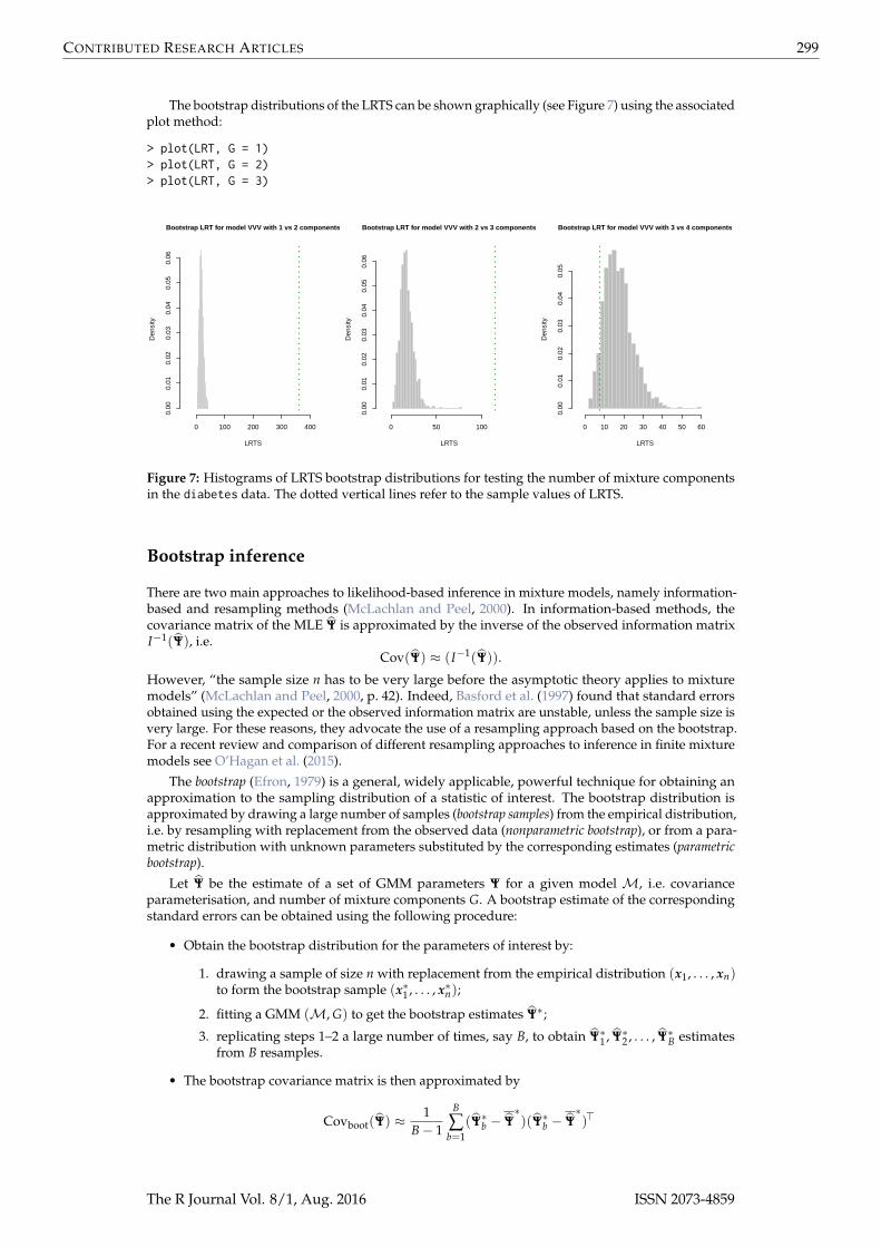
The bootstrap distributions of the LRTS can be shown graphically (see Figure 7) using the associatedplot method:

> plot(LRT, G = 1)> plot(LRT, G = 2)> plot(LRT, G = 3)

LRTS

Den

sity

0 100 200 300 400

0.00

0.01

0.02

0.03

0.04

0.05

0.06

Bootstrap LRT for model VVV with 1 vs 2 components

LRTS

Den

sity

0 50 100

0.00

0.01

0.02

0.03

0.04

0.05

0.06


LRTS

Den

sity

0 10 20 30 40 50 60

0.00

0.01

0.02

0.03

0.04

0.05


Figure 7: Histograms of LRTS bootstrap distributions for testing the number of mixture componentsin the diabetes data. The dotted vertical lines refer to the sample values of LRTS.

Bootstrap inference

There are two main approaches to likelihood-based inference in mixture models, namely information-based and resampling methods (McLachlan and Peel, 2000). In information-based methods, thecovariance matrix of the MLE Ψ is approximated by the inverse of the observed information matrixI−1(Ψ), i.e.

Cov(Ψ) ≈ (I−1(Ψ)).

However, “the sample size n has to be very large before the asymptotic theory applies to mixturemodels” (McLachlan and Peel, 2000, p. 42). Indeed, Basford et al. (1997) found that standard errorsobtained using the expected or the observed information matrix are unstable, unless the sample size isvery large. For these reasons, they advocate the use of a resampling approach based on the bootstrap.For a recent review and comparison of different resampling approaches to inference in finite mixturemodels see O’Hagan et al. (2015).

The bootstrap (Efron, 1979) is a general, widely applicable, powerful technique for obtaining anapproximation to the sampling distribution of a statistic of interest. The bootstrap distribution isapproximated by drawing a large number of samples (bootstrap samples) from the empirical distribution,i.e. by resampling with replacement from the observed data (nonparametric bootstrap), or from a para-metric distribution with unknown parameters substituted by the corresponding estimates (parametricbootstrap).

Let Ψ be the estimate of a set of GMM parameters Ψ for a given model M, i.e. covarianceparameterisation, and number of mixture components G. A bootstrap estimate of the correspondingstandard errors can be obtained using the following procedure:

• Obtain the bootstrap distribution for the parameters of interest by:

1. drawing a sample of size n with replacement from the empirical distribution (x1, . . . , xn)to form the bootstrap sample (x∗1 , . . . , x∗n);

2. fitting a GMM (M, G) to get the bootstrap estimates Ψ∗;

3. replicating steps 1–2 a large number of times, say B, to obtain Ψ∗1 , Ψ∗2 , . . . , Ψ∗B estimatesfrom B resamples.

• The bootstrap covariance matrix is then approximated by

Covboot(Ψ) ≈ 1B− 1

B

∑b=1

(Ψ∗b − Ψ∗)(Ψ∗b − Ψ

∗)>



where Ψ∗=

1B

B

∑b=1

Ψ∗b .

• The bootstrap standard errors for the parameter estimates Ψ are computed as the square root ofthe diagonal elements of the bootstrap covariance matrix, i.e.

seboot(Ψ) =√

diag(Covboot(Ψ)).

Consider the hemophilia dataset (Habbema et al., 1974) available in the package rrcov, whichcontains two measured variables on 75 women belonging to two groups: 30 of them are non-carriers(normal group) and 45 are known hemophilia A carriers (obligatory carriers).

> data(hemophilia, package = "rrcov")> X <- hemophilia[,1:2]> Class <- as.factor(hemophilia$gr)> plot(X, pch = ifelse(Class == "normal", 1, 16))> legend("bottomright", legend = levels(Class), pch = c(16,1), inset = 0.03)

The last command plots the observed data marked by the known classification (see Figure 8a).

In analogy with the analysis of Basford et al. (1997, example II, Sec. 5), we fitted a two-componentsGMM with unconstrained covariance matrices:

> mod <- Mclust(X, G = 2, modelName = "VVV")> summary(mod, parameters = TRUE)----------------------------------------------------Gaussian finite mixture model fitted by EM algorithm----------------------------------------------------

Mclust VVV (ellipsoidal, varying volume, shape, and orientation) model with 2 components:

log.likelihood n df BIC ICL77.02852 75 11 106.5647 92.85533

Clustering table:1 239 36

Mixing probabilities:1 2

0.5108084 0.4891916

Means:[,1] [,2]

AHFactivity -0.11627884 -0.36656353AHFantigen -0.02457577 -0.04534792

Variances:[,,1]

AHFactivity AHFantigenAHFactivity 0.01137602 0.00659927AHFantigen 0.00659927 0.01239353[,,2]

AHFactivity AHFantigenAHFactivity 0.01585986 0.01505449AHFantigen 0.01505449 0.03236079

Note that in the summary() function call we used the optional argument parameters = TRUE to retrievethe estimated parameters.

The clustering structure identified is shown in Figure 8b and can be obtained as follows:

> plot(mod, what = "classification", main = FALSE)

Bootstrap inference for GMMs is available through the function MclustBootstrap(), which re-quires the user to input an object returned by a call to Mclust(). Optionally, the user can also providethe number of bootstrap resamples nboot and the type of bootstrap to perform. By default, nboot =999 and type = "bs" for the nonparametric bootstrap. Thus, a simple call for computing the bootstrapdistribution of the GMM parameters is the following:



●●

●

●

●

●●

●

●

●

●

●

●

●

●

●

●

●

●

●

●

●

●

●●

●

●

●● ●

●

●

●

●

●

●

●

● ●

●

●

●

●

●

●

●

●

●

●

●

●

●

●

●

●

●

●

●

●

●

●

●●

●

●

●

●

● ●●

●

●

●

●

●

−0.6 −0.4 −0.2 0.0

−0.

4−

0.2

0.0

0.2

AHFactivity

AH

Fant

igen

●

●

carriernormal

(a)

−0.6 −0.4 −0.2 0.0

−0.

4−

0.2

0.0

0.2

AHFactivity

AH

Fant

igen

●●

●

●

●●

●

●

●

●

●

●

●

●

●

●

●

●

●

●

●●

●

●

●● ●

●

●

●

●

●

● ●●

●

●

●

●

(b)

Figure 8: True class membership (a) and estimated classification using GMM (b) for the hemophiliadataset.

> boot <- MclustBootstrap(mod, nboot = 999, type = "bs")

Note that for the sake of clarity we have included the arguments nboot and type, but they can beomitted since they are set at their defaults.

The function MclustBootstrap() returns an object which can be plotted or summarised. Forinstance, to graph the bootstrap distribution for the mixing proportions and for the component meanswe may use the code:

> par(mfrow = c(1,2))> plot(boot, what = "pro")> par(mfrow = c(2,2))> plot(boot, what = "mean")> par(mfrow = c(1,1))

The resulting plots are shown, respectively, in Figures 9 and 10.

Mix. prop. for comp. 1

0.0 0.2 0.4 0.6 0.8 1.0

050

100

150

Mix. prop. for comp. 2

0.0 0.2 0.4 0.6 0.8 1.0

050

100

150

Figure 9: Bootstrap distribution for the mixture proportions. The vertical dotted lines refer to theMLEs for the GMM fitted to the hemophilia data.

A numerical summary of the bootstrap procedure is available through the summary method, whichby default returns the standard errors of GMM parameters:

> summary(boot, what = "se")----------------------------------------------------------Resampling standard errors----------------------------------------------------------Model = VVV



AHFactivity mean for comp. 1

−0.6 −0.5 −0.4 −0.3 −0.2 −0.1 0.0

010

020

030

040

050

060

0

AHFactivity mean for comp. 2

−0.6 −0.5 −0.4 −0.3 −0.2 −0.1 0.0

010

020

030

040

050

0

AHFantigen mean for comp. 1

−0.3 −0.2 −0.1 0.0 0.1 0.2

050

100

150

200

250

AHFantigen mean for comp. 2

−0.3 −0.2 −0.1 0.0 0.1 0.2

010

020

030

0

Figure 10: Bootstrap distribution for the mixture component means. The vertical dotted lines refer tothe MLEs for the GMM fitted to the hemophilia data.

Num. of mixture components = 2Replications = 999Type = nonparametric bootstrap


0.1249357 0.1249357

Means:1 2

AHFactivity 0.04028375 0.04137370AHFantigen 0.03262182 0.06456482

Variances:[,,1]

AHFactivity AHFantigenAHFactivity 0.007018580 0.004690481AHFantigen 0.004690481 0.003155312[,,2]


The summary method can also return bootstrap percentile confidence intervals. For the genericGMM parameter ψ of Ψ, the percentile method yields the intervals [ψ∗α/2, ψ∗1−α/2], where ψ∗q is the qthquantile (or the 100qth percentile) of the bootstrap distribution (ψ∗1 , . . . , ψ∗B). These can be obtained byspecifying in the summary call the argument what = "ci" and, optionally, the confidence level of theintervals (by default, conf.level = 0.95). For instance:

> summary(boot, what = "ci")----------------------------------------------------------



Resampling confidence intervals----------------------------------------------------------Model = VVVNum. of mixture components = 2Replications = 999Type = nonparametric bootstrapConfidence level = 0.95


2.5% 0.3193742 0.178505497.5% 0.8214946 0.6806258

Means:[,,1]

AHFactivity AHFantigen2.5% -0.22915526 -0.0978499697.5% -0.07315876 0.02481681[,,2]

AHFactivity AHFantigen2.5% -0.4573113 -0.157162497.5% -0.2747451 0.1318332

Variances:[,,1]

AHFactivity AHFantigen2.5% 0.004743597 0.00701267297.5% 0.032144767 0.019245540[,,2]

AHFactivity AHFantigen2.5% 0.003981163 0.00604907697.5% 0.027297495 0.045854646

The function MclustBootstrap() has also the provision for using the weighted likelihood boot-strap (Newton and Raftery, 1994). This is a generalisation of the nonparametric bootstrap whichassigns random (positive) weights to sample observations; it can be viewed as a generalized Bayesianbootstrap. The weights are obtained from a uniform Dirichlet distribution, i.e. by sampling fromn independent standard exponential distributions and then rescaling by their average. Then, thefunction me.weighted() in mclust allows one to apply a weighted EM algorithm. This approachmay yield benefits when one or more components have small mixture proportions. In that case, anonparametric bootstrap sample may have no representatives of them, but the weighted likelihoodbootstrap will always have representatives of all groups.

In our data example the weighted likelihood bootstrap can be easily obtained by specifying type= "wlbs" in the MclustBootstrap() function call:

> wlboot <- MclustBootstrap(mod, nboot = 999, type = "wlbs")> summary(wlboot, what = "se")----------------------------------------------------------Resampling standard errors----------------------------------------------------------Model = VVVNum. of mixture components = 2Replications = 999Type = weighted likelihood bootstrap


0.1323612 0.1323612

Means:1 2

AHFactivity 0.03977347 0.04192182AHFantigen 0.02989056 0.06897928

Variances:



[,,1]AHFactivity AHFantigen

AHFactivity 0.007074450 0.004686432AHFantigen 0.004686432 0.003254011[,,2]


In this case the differences between the nonparametric and the weighted likelihood bootstrap arenegligible. We can summarise the inference for the components means obtained under the twoapproaches with the following graphs of bootstrap percentile confidence intervals:

> boot.ci <- summary(boot, what = "ci")> wlboot.ci <- summary(wlboot, what = "ci")> par(mfrow = c(1,2), mar = c(4,4,1,1))> for(j in 1:mod$G)

{ plot(1:mod$G, mod$parameters$mean[j,], col = 1:mod$G, pch = 15,ylab = colnames(X)[j], xlab = "Mixture component",ylim = range(boot.ci$mean,wlboot.ci$mean),xlim = c(.5,mod$G+.5), xaxt = "n")

points(1:mod$G+0.2, mod$parameters$mean[j,], col = 1:mod$G, pch = 15)axis(side = 1, at = 1:mod$G)with(boot.ci, errorBars(1:G, mean[1,j,], mean[2,j,], col = 1:G))with(wlboot.ci, errorBars(1:G+0.2, mean[1,j,], mean[2,j,], col = 1:G, lty = 2))

}> par(mfrow = c(1,1))

−0.

4−

0.3

−0.

2−

0.1

0.0

0.1

Mixture component

AH

Fact

ivity

1 2

−0.

4−

0.3

−0.

2−

0.1

0.0

0.1

Mixture component

AH

Fant

igen

1 2

Figure 11: Bootstrap percentile intervals for the means of the GMM fitted to the hemophilia dataset.Solid lines refer to nonparametric bootstrap, dashed lines to the weighted likelihood bootstrap.

Initialisation of the EM algorithm

The EM algorithm is an easy to implement and numerically stable algorithm which has reliable globalconvergence under fairly general conditions. However, the likelihood surface in mixture models tendsto have multiple modes and thus initialisation of EM is crucial because it usually produces sensibleresults when started from reasonable starting values (Wu, 1983).

In mclust the EM algorithm is initialised using the partitions obtained from model-based hier-archical agglomerative clustering (MBHAC). In this approach, hierarchical clusters are obtained byrecursively merging the two clusters that provide the smallest decrease in the classification likeli-hood for Gaussian mixture model (Banfield and Raftery, 1993). Efficient numerical algorithms havebeen discussed by Fraley (1998). Using MBHAC is particularly convenient because the underlyingprobabilistic model is shared by both the initialisation step and the model fitting step. Furthermore,MBHAC is also computationally advantageous because a single run provides the basis for initialisingthe EM algorithm for any number of mixture components and component-covariances parameterisa-



tions. Although there is no guarantee that the EM initialized by MBHAC will converge to the globaloptimum, it often provides reasonable starting points.

A problem with the MBHAC approach may arise in the presence of coarse data, resulting from thediscrete nature of the data or from continuous data that are rounded when measured. In this case, tiesmust be broken by choosing the pair of entities that will be merged. This is often done at random, butregardless of which method is adopted for breaking ties, this choice can have important consequencesbecause it changes the clustering of the remaining observations. Moreover, the final EM solution maydepend on the ordering of the variables.

Consider the Flea beetles data available in package tourr. This dataset provides six physicalmeasurements for a sample of 72 flea beetles from three species:

> data(flea, package = "tourr")> X <- data.matrix(flea[,1:6])> Class <- factor(flea$species, labels = c("Concinna","Heikertingeri","Heptapotamica"))> table(Class)Class

Concinna Heikertingeri Heptapotamica21 31 22

> col <- mclust.options("classPlotColors")[1:3]> clp <- clPairs(X, Class, lower.panel = NULL, gap = 0,

symbols = c(16,15,17), colors = adjustcolor(col, alpha.f = 0.5))> clPairsLegend(x = 0.1, y = 0.3, class = clp$class, col = col, pch = clp$pch,

title = "Flea beatle species")

As can be seen from Figure 12, the observed values are rounded (to the nearest integer presumably)and there is a strong overplotting of points.

120 160 200 240

120

160

200

240

tars1

110 130 45 50 55 120 140 8 10 12 14 16 60 80 100

120

160

200

240

tars211

013

0

head

4550

55

aede1

120

140

aede2

810

14

60 80 100

6080

100

aede3

●

Flea beatle species

Concinna

Heikertingeri

Heptapotamica

Figure 12: Scatterplot matrix for the Flea beetles data with points marked according to the true classes.

> mod1 <- Mclust(X)> summary(mod1)----------------------------------------------------Gaussian finite mixture model fitted by EM algorithm----------------------------------------------------

Mclust EEE (ellipsoidal, equal volume, shape and orientation) model with 5 components:




Clustering table:1 2 3 4 521 2 20 20 11> adjustedRandIndex(Class, mod1$classification)[1] 0.7675713

> mod2 <- Mclust(X[,6:1])> summary(mod2)----------------------------------------------------Gaussian finite mixture model fitted by EM algorithm----------------------------------------------------



Clustering table:1 2 3 4 522 21 22 7 2> adjustedRandIndex(Class, mod2$classification)[1] 0.8131206

By reversing the order of the variables in the fit of mod2, the initial partitions differ due to ties in thedata, so the EM algorithm converges to different solutions of the same EEE model with 5 components.The second solution has a higher BIC and better accuracy.

In situations like this we may want to assess the stability of results by randomly starting theEM algorithm. The function randomPairs() may be called to obtain a random hierarchical structuresuitable to be used as initial clustering partition:

> mod3 <- Mclust(X, initialization = list(hcPairs = randomPairs(X, seed = 123)))> summary(mod3)----------------------------------------------------Gaussian finite mixture model fitted by EM algorithm----------------------------------------------------



Clustering table:1 2 3 416 15 22 21> adjustedRandIndex(Class, mod3$classification)[1] 0.7867056

Using a random start we obtain a EEE model with 4 components, which has a higher BIC but a lowerARI. However, a better initialisation may be found using the approach discussed in Scrucca andRaftery (2015). The main idea is to project the data through a suitable transformation which enhancesseparation among clusters before applying the MBHAC at the initialisation step. Once a reasonablehierarchical partition is obtained, the EM algorithm is run using the data on the original scale. Forinstance, a GMM started using the scaled SVD transformation is obtained with the following code:

> mod4 <- Mclust(X, initialization = list(hcPairs = hc(X, use = "SVD")))> summary(mod4)----------------------------------------------------Gaussian finite mixture model fitted by EM algorithm----------------------------------------------------



Clustering table:



1 2 321 31 22> adjustedRandIndex(Class, mod4$classification)[1] 1

In this case we achieve both the highest BIC and a perfect classification of the fleas into the actualspecies.

We conclude by noting that in the case of large datasets, i.e. having a large number of observationsor cases, a subsample of the data can be used in the MBHAC phase before applying the EM algorithmto the full data set. This is easily done by providing an optional argument to Mclust() or mclustBIC()(as well as many other functions) as a vector, say s, of logical values or numerical indices specifyingthe subset of data to be used in the initial hierarchical clustering phase:

> Mclust(X, initialization = list(subset = s))

Density estimation

Density estimation plays an important role in applied statistical data analysis and theoretical research.Finite mixture models provide a flexible semi-parametric model-based approach to density estimation,which makes it possible to accurately approximate any given probability distribution. mclust providesa simple interface to Gaussian mixture models for univariate and multivariate density estimation.

Izenman and Sommer (1988) considered the fitting of a Gaussian mixture to the distribution of thethickness of stamps in the 1872 Hidalgo stamp issue of Mexico 2. A density estimate based on GMMcan be obtained using the function densityMclust():

> data(Hidalgo1872, package = "MMST")> Thickness <- Hidalgo1872$thickness> Year <- rep(c("1872", "1873-74"), c(289, 196))> dens <- densityMclust(Thickness)> summary(dens$BIC)Best BIC values:

V,3 V,5 V,4BIC 2983.791 2974.939223 2972.19349BIC diff 0.000 -8.852019 -11.59775> summary(dens, parameters = TRUE)-------------------------------------------------------Density estimation via Gaussian finite mixture modeling-------------------------------------------------------

Mclust V (univariate, unequal variance) model with 3 components:

log.likelihood n df BIC ICL1516.632 485 8 2983.791 2890.914


128 171 186

Mixing probabilities:1 2 3

0.2661410 0.3011217 0.4327374

Means:1 2 3

0.07215458 0.07935341 0.09919740

Variances:1 2 3

0.000004814927 0.000003097694 0.000188461484

2The Hidalgo stamp data is available at the home page for the book by Izenman (2008) at http://astro.temple.edu/~alan/MMST/datasets.html, or through the package MMST. The latter has been archived on CRAN, so itmust be installed using the following code:

> install.packages("http://cran.r-project.org/src/contrib/Archive/MMST/MMST_0.6-1.1.tar.gz", repos= NULL, type = "source")


http://astro.temple.edu/~alan/MMST/datasets.html

http://astro.temple.edu/~alan/MMST/datasets.html


The model selected is a three-component mixture with different variances. A graph of the densityestimated is shown in Figure13a and is obtained with the code:

> br <- seq(min(Thickness), max(Thickness), length = 21)> plot(dens, what = "density", data = Thickness, breaks = br)

Here a histogram of the observed data is also drawn by providing the optional argument data andwith breakpoints between histogram cells specified in the argument breaks. From the graph, threemodes appear at the means of the mixture components: one with larger stamp thickness, and twocorresponding to thinner stamps.

Additional information can also be used. In particular, thickness measurements can be groupedaccording to the year of consignment; the first 289 stamps refer to the 1872 issue, and the remaining196 stamps to the years 1873–1874. We may draw a (suitable scaled) histogram for each year-of-consignment and then add the estimated components densities as follows:

> h1 <- hist(Thickness[Year == "1872"], breaks = br, plot = FALSE)> h1$density <- h1$density*prop.table(table(Year))[1]> h2 <- hist(Thickness[Year == "1873-74"], breaks = br, plot = FALSE)> h2$density <- h2$density*prop.table(table(Year))[2]> x <- seq(min(Thickness)-diff(range(Thickness))/10,

max(Thickness)+diff(range(Thickness))/10, length = 200)> cdens <- predict(dens, x, what = "cdens")> cdens <- t(apply(cdens, 1, function(d) d*dens$parameters$pro))> col <- adjustcolor(mclust.options("classPlotColors")[1:2], alpha = 0.3)> plot(h1, xlab = "Thickness", freq = FALSE, main = "", border = FALSE, col = col[1],

xlim = range(x), ylim = range(h1$density, h2$density, cdens))> plot(h2, add = TRUE, freq = FALSE, border = FALSE, col = col[2])> matplot(x, cdens, type = "l", lwd = 1, add = TRUE, lty = 1:3, col = 1)> box()

The result is shown in Figure 13b. Stamps from 1872 show a two-regime distribution, with onecorresponding to the component with the largest thickness, and one whose distribution essentiallyoverlaps with the bimodal distribution of stamps for the years 1873–1874.

Thickness

Den

sity

0.06 0.08 0.10 0.12 0.14

020

4060

(a)Thickness

Den

sity

0.06 0.08 0.10 0.12 0.14

010

2030

4050

6070

(b)

Figure 13: (a) Histogram with mixture-based density estimate curve, and (b) histograms by group-yearwith estimated mixture-component densities, for the Hidalgo1872 stamps dataset.

As an example of bivariate density estimation, consider the well-known ‘Old Faithful’ data setwhich provides the waiting time between eruptions (waiting) and the duration of the eruptions(eruptions) for the Old Faithful geyser in Yellowstone National Park, Wyoming, USA. The datasetcan be read and data plotted as follows:

> data(faithful)> plot(faithful, cex = 0.5)

A bivariate density estimate for the Faithful data is obtained with the commands:

> dens <- densityMclust(faithful)> summary(dens)



●

●

●

●

●

●

●

●

●

●

●

●

●

●

●

●

●

●

●

●

●

●

●

●

●

●

●

●

●

●

●

●

●

●

●

●

●

●

●

●

●

●

●

●

●

●

●

●

●

●

●

●

●

●

●

●

●

●

●

●

●

●

●

●

●

●

● ●

●

●

●

●

●

●

●

●

●

●

●

●

●

●

●

●

●

●

●

●

●

●

●

●

●

●

●

●

●

●

●

●

●

●

●

●

●

●

●

●

●

●

●

●

●

●

●

●

●

●

●

●

●

●

●

●

●

●

●

●

●

●

●

●

●

●

●

●

●

●

●

●

●

●

●

●

●

●

●

●

●

●

●●

●

●

●

●

●

●

●

●

●

●

●

●

●

●

●

●

●

●

●

●

●

●

● ●

●

●

●

●

●

●

●●

●

●

●

●

●

●

●

●

●

●

●

●

●

●

●

●

●

●

●

●

●

●

●

●

●

●

●

●

●

●

●

●

●

●

●

●

●

●

●

●

●

●

● ●

●

●

●

●

●

●

●

●●

●

●

●

●

●

●

●

●

●

●

●

●

●

●

●

● ●

●

●

●

●

●

●

●

●

●

●

●

●

●

●

●

●

●

●

1.5 2.0 2.5 3.0 3.5 4.0 4.5 5.0

5060

7080

90

eruptions

wai

ting

(a)eruptions

wai

ting

1.5 2.0 2.5 3.0 3.5 4.0 4.5 5.0

5060

7080

90

●

●

●

●

●

●

●

●

●

●

●

●

●

●

●

●

●

●

●

●

●

●

●

●

●

●

●

●

●

●

●

●

●

●

●

●

●

●

●

●

●

●

●

●

●

●

●

●

●

●

●

●

●

●

●

●

●

●

●

●

●

●

●

●

●

●

● ●

●

●

●

●

●

●

●

●

●

●

●

●

●

●

●

●

●

●

●

●

●

●

●

●

●

●

●

●

●

●

●

●

●

●

●

●

●

●

●

●

●

●

●

●

●

●

●

●

●

●

●

●

●

●

●

●

●

●

●

●

●

●

●

●

●

●

●

●

●

●

●

●

●

●

●

●

●

●

●

●

●

●

●●

●

●

●

●

●

●

●

●

●

●

●

●

●

●

●

●

●

●

●

●

●

●

● ●

●

●

●

●

●

●

●●

●

●

●

●

●

●

●

●

●

●

●

●

●

●

●

●

●

●

●

●

●

●

●

●

●

●

●

●

●

●

●

●

●

●

●

●

●

●

●

●

●

●

● ●

●

●

●

●

●

●

●

●●

●

●

●

●

●

●

●

●

●

●

●

●

●

●

●

● ●

●

●

●

●

●

●

●

●

●

●

●

●

●

●

●

●

●

●

(b)

2.0 2.5 3.0 3.5 4.0 4.5 5.0

5060

7080

90

eruptions

wai

ting

(c)

eruptions

waiting

Density

(d)

Figure 14: Plot of the Old Faithful data (a), mixture-based density estimate contours (b), image plot ofdensity estimate (c) and perspective plot of the bivariate density estimate (d).

-------------------------------------------------------Density estimation via Gaussian finite mixture modeling-------------------------------------------------------




130 97 45

Model selection based on the BIC selects a three-component mixture with common covariance matrix(EEE). One component is used to model the group of observations having both low duration and lowwaiting times, whereas two components are needed to approximate the skewed distribution of theobservations with larger duration and waiting times.

Figure 14b-d shows some of the available graphs in mclust for a bivariate density estimated byGMM. These can be obtained with the commands:

> plot(dens, what = "density", data = faithful, grid = 200, points.cex = 0.5,drawlabels = FALSE)

> plot(dens, what = "density", type = "image", col = "steelblue", grid = 200)> plot(dens, what = "density", type = "persp", theta = -25, phi = 20,

border = adjustcolor(grey(0.1), alpha.f = 0.3))

Note that the same procedure using the function mclustDensity() can also be used to obtaindensity estimates for higher dimensional datasets.



Supervised classification

In supervised classification or discriminant analysis the aim is to build a classifier (or a decision rule)which is able to assign an observation with an unknown class membership to one of K known classes.For building a supervised classifier, a training dataset {(x1, y1), . . . , (xn, yn)} is used for which boththe features xi and true classes yi ∈ {C1, . . . , CK} are known.

Mixture-based discriminant analysis models assume that the density for each class follows aGaussian mixture distribution

fk(x) =Gk

∑g=1

πgkφ(x; µgk, Σgk),

where πgk are the mixing probabilities for class k (πgk > 0, ∑Gkg=1 πgk = 1), µgk the means for component

g within class k, and Σgk the covariance matrix of component g within class k. Hastie and Tibshirani(1996) proposed Mixture Discriminant Analysis (MDA) where it is assumed that the covariance matrixis the same for all the classes but is otherwise unconstrained, i.e. Σgk = Σ for all g and k. The numberof mixture components is assumed known for each class.

Bensmail and Celeux (1996) proposed the Eigenvalue Decomposition Discriminant Analysis(EDDA) which assumes that the density for each class can be described by a single Gaussian component(i.e. Gk = 1 for all k) with the component covariance structure factorised as

Σk = λkDk AkD>k .

Several models can be obtained from the above decomposition. If Σk = λDAD> (model EEE), thenEDDA is equivalent to linear discriminant analysis (LDA). If Σk = λkDk AkD>k (model VVV) thenEDDA is equivalent to quadratic discriminant analysis (QDA).

Consider the UCI Wisconsin breast cancer diagnostic data available at http://archive.ics.uci.edu/ml/datasets/Breast+Cancer+Wisconsin+(Diagnostic). This dataset provides data for 569patients on 30 features of the cell nuclei obtained from a digitized image of a fine needle aspirate (FNA)of a breast mass (Mangasarian et al., 1995). For each patient the cancer was diagnosed as malignantor benign. Following Fraley and Raftery (2002) we considered only three attributes: extreme area,extreme smoothness, and mean texture. The dataset can be downloaded from the UCI repositoryusing the following commands:

> data <- read.csv("http://archive.ics.uci.edu/ml/machine-learning-databases/breast-cancer-wisconsin/wdbc.data", header = FALSE)> X <- data[,c(4, 26, 27)]> colnames(X) <- c("texture.mean", "area.extreme", "smoothness.extreme")> Class <- data[,2]

Then, we may randomly assign approximately 2/3 of the observations to the training set, and theremaining ones to the test set:

> set.seed(123)> train <- sample(1:nrow(X), size = round(nrow(X)*2/3), replace = FALSE)> X.train <- X[train,]> Class.train <- Class[train]> table(Class.train)Class.trainB M

238 141> X.test <- X[-train,]> Class.test <- Class[-train]> table(Class.test)Class.testB M

119 7 1

The function MclustDA() provides fitting capabilities for the EDDA model, but we must specifythe optional argument modelType = "EDDA". The function call is thus the following:

> mod1 <- MclustDA(X.train, Class.train, modelType = "EDDA")> summary(mod1, newdata = X.test, newclass = Class.test)------------------------------------------------Gaussian finite mixture model for classification------------------------------------------------


http://archive.ics.uci.edu/ml/datasets/Breast+Cancer+Wisconsin+(Diagnostic)

http://archive.ics.uci.edu/ml/datasets/Breast+Cancer+Wisconsin+(Diagnostic)


EDDA model summary:

log.likelihood n df BIC-2989.967 379 12 -6051.185

Classes n Model GB 238 VVI 1M 141 VVI 1

Training classification summary:

PredictedClass B M

B 237 1M 19 122

Training error = 0.05277045

Test classification summary:

PredictedClass B M

B 116 3M 5 66

Test error = 0.04210526

The EDDA mixture model selected by BIC is the VVI model, so each group is described by asingle Gaussian component with varying volume and shape, but same orientation aligned with thecoordinate axes. Note that in the summary() function call we also provided the features and the knownclasses for the test set, so both the training error and the test error are reported. A cross-validationerror can also be computed using the cvMclustDA() function, which by default use nfold = 10 for a10-fold cross-validation:

> cv <- cvMclustDA(mod1)> unlist(cv[c("error", "se")])

error se0.052770449 0.007930516

EDDA imposes a single mixture component for each group. However, in certain circumstancesmore complexity may improve performance. A more general approach, called MclustDA, has beenproposed by Fraley and Raftery (2002), where a finite mixture of Gaussian distributions is used withineach class, with number of components and covariance matrix structures (expressed following theusual decomposition) being different between classes. This is the default model fitted by MclustDA:

> mod2 <- MclustDA(X.train, Class.train)> summary(mod2, newdata = X.test, newclass = Class.test)------------------------------------------------Gaussian finite mixture model for classification------------------------------------------------

MclustDA model summary:


Classes n Model GB 238 EEV 2M 141 VVI 2


PredictedClass B M

B 236 2



M 7 134



PredictedClass B M

B 114 5M 2 69

Test error = 0.03684211

A two-component mixture distribution is fitted to both the benign and malignant observations, butwith different covariance structures within each class. Both the training error and the test error areslightly smaller than for EDDA, a fact also confirmed by the 10-fold cross-validation procedure:

> cv <- cvMclustDA(mod2)> unlist(cv[c("error", "se")])

error se0.021108179 0.007648168

A plot method which produces a variety of graphs is associated with objects returned by MclustDA.For instance, pairwise scatterplots between the features, showing both the known classes and theestimated mixture components, are drawn as follows (see Figure 15a–c):

> plot(mod2, what = "scatterplot", dimens = c(1,2))> plot(mod2, what = "scatterplot", dimens = c(2,3))> plot(mod2, what = "scatterplot", dimens = c(3,1))

Another interesting graph can be obtained by projecting the data on a dimension reduced subspace(Scrucca, 2014) with the commands:

> drmod2 <- MclustDR(mod2)> summary(drmod2)-----------------------------------------------------------------Dimension reduction for model-based clustering and classification-----------------------------------------------------------------

Mixture model type: MclustDA

Classes n Model GB 238 EEV 2M 141 VVI 2

Estimated basis vectors:Dir1 Dir2 Dir3

texture.mean -0.00935540 -0.044384467 -0.0006607120area.extreme 0.00049997 0.000071676 -0.0000088494smoothness.extreme 0.99995611 -0.999014521 0.9999997817

Dir1 Dir2 Dir3Eigenvalues 0.67718 0.28159 0.013928Cum. % 69.61869 98.56810 100.000000> plot(drmod2, what = "boundaries", ngrid = 200)

The graph produced by the last command is shown in Figure 15d. The two groups are largely separatedalong the first direction, with the group of malignant cases showing a higher variability.

Finally, note that the MDA model is equivalent to MclustDA with Σk = λDAD> (model EEE) andfixed Gk ≥ 1 for each k = 1, . . . , K. For instance, a MDA with two mixture components for each classcan be fitted as:

> mod3 <- MclustDA(X.train, Class.train, G = 2, modelNames = "EEE")> summary(mod3, newdata = X.test, newclass = Class.test)------------------------------------------------Gaussian finite mixture model for classification------------------------------------------------



10 15 20 25 30 35 40

1000

2000

3000

4000

texture.mean

area

.ext

rem

e

●

●

●●

●

●

●

●

●

●

● ●

●●●

● ●●●

● ●● ●● ●

●

●

●

●●

●●

●

●

● ●

●●

●● ●

●●

●

● ●

●

●●

●●●

●

●

●

●

●●

● ●●

● ●

●●

●●

●●

●

●●

●●●

●

●●

●●

● ●●● ●

●

● ●

●

●

●●

●

●

●●

●

●

●●

●

●

●

●●

●●

●●●

●●

●

●

●

●●

●

●●

●

●

●

●●●

●●

● ●●

●

●

●

● ●●

● ●

●

●

●

●

●●

●

●●

●●

●●●

●

●

●

●

●

●●

● ●●

●●

●

●

●

●

●

●● ●●

●●

●

●● ●

● ● ●

●●

●

●

●

●

●

●

●

●●

●

●

●●

●

●

●

●

●●●

●

●

●●

●●

●

●●

●

●

●

●

●●

●●

●

●

●

●

●●●

●

●

●

●●

●

●

●●

(a)

1000 2000 3000 4000

0.08

0.10

0.12

0.14

0.16

0.18

0.20

0.22

area.extreme

smoo

thne

ss.e

xtre

me

●

●

●

●

●

●

●

●

●

●

●

●

●

●●

●

●

●

●

●●

●

●

●

●

●

● ●

●

●

●

●

●

●

●

●

●●

●

●

●

●

●

●●

●

●

●

●

●

●

●

●

●●

● ●●

●

●●

●

●

●

●

●

●

●

●

●

●

●

●

●

●

●

●

●

●●●

●●

●

●

●

●

●

●

●●

●

●

●

●

●

●

●

●

●

●

●●

●

●●

●

●

●

●

●

●

●

●

●

●●

●

●

●

●

●

●

●

●

●

●

●

●

●

●

●

●

●

●

●

●

●

●

●

●

●

●

●

●

●

●

● ●

●●

●

●

●

●

●

●

●

●●

●

●

●●

●

●

●

●

●

●

●

●

●

●●

●

●

●

●

●

●

●

●

●●

●

●

● ●

●

●

●

●

●●

●

●

●

●

●

●

●

●

●●

●

●

●

●

●

●●

●

●

●

●●

●

●

●

●

●

●

●

●

●●

●

●

●

●

●

●

●

●●

● ●

(b)

0.08 0.10 0.12 0.14 0.16 0.18 0.20 0.22

1015

2025

3035

40

smoothness.extreme

text

ure.

mea

n

●

●

●

●

●

●

●

●

●●

●●

●

●

● ●

●

●●

●

●

●

●

●

●

●

●●

●

●

●

●

●

●

●●

●

●

●

●

●

●

●

●

●

●

●

●

●

● ●

●

●

●

●

●

●

●

●

●

●

●

●

●

●

●

●

●

●

●

●

●

●

●

●

●

●

●

●●

●

●

●

●

●

●●

●

●

●

●

●

●

●

●

●

●

●

●

●

●

●

●

●

●

●

●

●

●

●

●

●●

●

●

●

●

●

●

●

●

●●

●

●

●●

●

●

●

●

●

●

●

●

●

● ●

●

●

●

●●

●

●

●

●

●

●

●

●

●

●

●

●

●

●

●●

●

●

●

●●

●

●●

●

●●

●

●

●●

●

●

●

●

●

●

●

●

●

●

●

●

●

●●

●●

●

●

●

●

●

●

●

●

●

●

●

●●●

●●

●

●

●

●

●

●

●

●

●

●

●

●

●● ●

●●

●

●

●●●

●●

●

●

●

●

●

●

●

(c)

0.0 0.5 1.0 1.5

−0.

8−

0.6

−0.

4−

0.2

0.0

0.2

0.4

Dir1

Dir2

●

●

●

●

●

●

●

●

●●●●

●

●

●

●

●●

●●

●

●

●

●

●

●●

●

● ●

●

●

●

●●

●

●

●

●

●●

●

●

●

●

●

●

●

●

●●

●

●

●

●●

●

●

●

●

●

●

●

●

●

●

●

●

●

●●

●

●

●

●

●

●

●

●●

●

●

●

●

●

●

●●

●

●

●

●

●

●

●

●

●●●

●

●

●

●

●

●

●

●

●

●

●

●

●●

●

●

●

●

●

●

●

●

●

●

●

●

● ●

●

●

●

●

●

●

●

●

●

● ●

●

●

●

●●

●

●

●

●

●

●

●

●

●

●

●

●

●

●

●●

●

●

●

●

●

●

●

●

●●

●

●

●

●●

●

●

●

●

●

●

●

●

●

●

●●

●

● ●

●

●

●

●

●

●

●

●

●

●

●

●

●

●

●●

●●

●

●

●

●

●

●

●

●

●

●

●

●

●●

●

● ●●●

●●●

●●

●

●

●

●

●

●

●

(d)

Figure 15: Pairwise scatterplots between variables for the Wisconsin breast cancer data (panels a–c).Points are marked by cancer diagnosis (benign = •, malignant = �), whereas ellipses correspond tocovariances of mixture components estimated with MclustDA. Plot of data projected along the first twoestimated directions obtained with MclustDR, and uncertainty classification boundaries (d).

MclustDA model summary:


Classes n Model GB 238 EEE 2M 141 EEE 2


PredictedClass B M

B 235 3M 12 129



PredictedClass B M

B 113 6



M 2 69

Test error = 0.04210526

Summary

mclust is one of the most popular R packages for Gaussian mixture modelling. Since its earlydevelopments (Banfield and Raftery, 1993; Fraley and Raftery, 1998, 1999), mclust has seen majorupdates through the years, which expanded its capabilities and features, increasing its popularity andwidening its area of utilisation.

Here we have presented the most salient new features introduced in version ≥ 5, namely newcovariance parameterisations, subspace data visualisation, different model selection criteria, bootstrap-based inference and EM algorithm initialisation. We showed their application on a collection ofdifferent datasets, pointing out their utility in different contexts.

Acknowledgments

Michael Fop and T. Brendan Murphy were supported by the Science Foundation Ireland fundedInsight Research Centre (SFI/12/RC/2289). Adrian E. Raftery and Luca Scrucca were supported byNIH grants R01 HD054511, R01 HD070936 and U54 HL127624.

Bibliography

J. S. Ahlquist and C. Breunig. Model-based clustering and typologies in the social sciences. PoliticalAnalysis, 20(1):92–112, 2012. [p289]

M. Aitkin and D. B. Rubin. Estimation and hypothesis testing in finite mixture models. Journal of theRoyal Statistical Society: Series B (Statistical Methodology), 47(1):67–75, 1985. [p295]

J. Banfield and A. E. Raftery. Model-based Gaussian and non-Gaussian clustering. Biometrics, 49:803–821, 1993. [p291, 304, 314]

K. E. Basford, D. R. Greenway, G. J. McLachlan, and D. Peel. Standard errors of fitted componentmeans of normal mixtures. Computational Statistics, 12(1):1–18, 1997. [p299, 300]

T. Benaglia, D. Chauveau, D. R. Hunter, and D. Young. mixtools: An R package for analyzing finitemixture models. Journal of Statistical Software, 32(6):1–29, 2009. URL http://www.jstatsoft.org/v32/i06/. [p289]

H. Bensmail and G. Celeux. Regularized Gaussian discriminant analysis through eigenvalue decom-position. Journal of the American Statistical Association, 91:1743–1748, 1996. [p310]

P. Biecek, E. Szczurek, M. Vingron, and J. Tiuryn. The R package bgmm: Mixture modeling withuncertain knowledge. Journal of Statistical Software, 47(3):1–32, 2012. URL http://www.jstatsoft.org/v47/i03/. [p289]

C. Biernacki, G. Celeux, and G. Govaert. Assessing a mixture model for clustering with the integratedcompleted likelihood. IEEE Transactions on Pattern Analysis and Machine Intelligence, 22(7):719–725,2000. [p295, 297]

S. Brin and L. Page. The anatomy of a large-scale hypertextual Web search engine. In Proceedings of theSeventh International Conference on World Wide Web, pages 107–117, 1998. [p290]

R. P. Browne and P. D. McNicholas. Estimating common principal components in high dimensions.Advances in Data Analysis and Classification, 8(2):217–226, 2014. [p291]

R. P. Browne, A. ElSherbiny, and P. D. McNicholas. mixture: Mixture Models for Clustering and Classifica-tion, 2015. URL https://CRAN.R-project.org/package=mixture. R package version 1.4. [p289]

J. G. Campbell, C. Fraley, D. Stanford, F. Murtagh, and A. E. Raftery. Model-based methods for textilefault detection. International Journal of Imaging Systems and Technology, 10(4):339–346, 1999. [p289]

G. Celeux and G. Govaert. Gaussian parsimonious clustering models. Pattern Recognition, 28:781–793,1995. [p291]


http://www.jstatsoft.org/v32/i06/




https://CRAN.R-project.org/package=mixture


W.-C. Chen and R. Maitra. EMCluster: EM Algorithm for Model-Based Clustering of Finite MixtureGaussian Distribution, 2015. URL https://CRAN.R-project.org/package=EMCluster. R packageversion 0.2-5. [p289]

G. Csardi. cranlogs: Download Logs from the RStudio CRAN Mirror, 2015. URL https://github.com/metacran/cranlogs. R package version 2.0.0. [p289]

G. Csardi and T. Nepusz. The igraph software package for complex network research. InterJournal,Complex Systems:1695, 2006. URL http://igraph.org. [p290]

A. P. Dempster, N. M. Laird, and D. B. Rubin. Maximum likelihood from incomplete data via the EMalgorithm. Journal of the Royal Statistical Society: Series B (Statistical Methodology), 39(1):1–38, 1977.[p291]

B. Efron. Bootstrap methods: Another look at the jackknife. The Annals of Statistics, 7:1–26, 1979. [p299]

K. J. Ellefsen, D. B. Smith, and J. D. Horton. A modified procedure for mixture-model clustering ofregional geochemical data. Applied Geochemistry, 51:315–326, 2014. [p289]

A. Flynt and M. I. G. Daepp. Diet-related chronic disease in the northeastern United States: Amodel-based clustering approach. International Journal of Health Geographics, 14(1):1–14, 2015. [p289]

C. Fraley. Algorithms for model-based Gaussian hierarchical clustering. SIAM Journal on ScientificComputing, 20(1):270–281, 1998. [p304]

C. Fraley and A. E. Raftery. How many clusters? Which clustering method? Answers via model-basedcluster analysis. The Computer Journal, 41:578–588, 1998. [p294, 295, 314]

C. Fraley and A. E. Raftery. MCLUST: Software for model-based cluster analysis. Journal of Classification,16(2):297–306, 1999. [p290, 314]

C. Fraley and A. E. Raftery. Model-based clustering, discriminant analysis, and density estimation.Journal of the American Statistical Association, 97(458):611–631, 2002. [p310, 311]

C. Fraley and A. E. Raftery. Enhanced model-based clustering, density estimation, and discriminantanalysis software: Mclust. Journal of Classification, 20(2):263–286, 2003. [p290]

C. Fraley and A. E. Raftery. Some applications of model-based clustering in chemistry. R News, 6(3):17–23, 2006a. URL http://CRAN.R-project.org/doc/Rnews/Rnews_2006-3.pdf. [p289]

C. Fraley and A. E. Raftery. Model-based microarray image analysis. R News, 6(5):60–63, 2006b. URLhttp://CRAN.R-project.org/doc/Rnews/Rnews_2006-5.pdf. [p289]

C. Fraley and A. E. Raftery. Bayesian regularization for normal mixture estimation and model-basedclustering. Journal of Classification, 24(2):155–181, 2007a. [p296]

C. Fraley and A. E. Raftery. Model-based methods of classification: Using the mclust software inchemometrics. Journal of Statistical Software, 18(6):1–13, 2007b. URL http://www.jstatsoft.org/v018/i06/. [p289]

C. Fraley, A. E. Raftery, T. B. Murphy, and L. Scrucca. MCLUST version 4 for R: Normal mixturemodeling for model-based clustering, classification, and density estimation. Technical Report 597,Department of Statistics, University of Washington, 2012. [p290, 296]

C. Fraley, A. E. Raftery, and L. Scrucca. mclust: Gaussian Mixture Modelling for Model-Based Clustering,Classification, and Density Estimation, 2016. URL https://CRAN.R-project.org/package=mclust. Rpackage version 5.2. [p289]

B. Grün and F. Leisch. Fitting finite mixtures of generalized linear regressions in R. ComputationalStatistics & Data Analysis, 51(11):5247–5252, 2007. [p289]

B. Grün and F. Leisch. FlexMix version 2: Finite mixtures with concomitant variables and varying andconstant parameters. Journal of Statistical Software, 28(4):1–35, 2008. URL http://www.jstatsoft.org/v28/i04/. [p289]

J. D. F. Habbema, J. Hermans, and K. van den Broek. A stepwise discriminant analysis program usingdensity estimation. In Proceedings in Computational Statistics, pages 101–110, Vienna: Physica-Verlag,1974. COMPSTAT. [p300]

T. Hastie and R. Tibshirani. Discriminant analysis by Gaussian mixtures. Journal of the Royal StatisticalSociety: Series B (Statistical Methodology), 58(1):155–176, 1996. [p310]


https://CRAN.R-project.org/package=EMCluster

https://github.com/metacran/cranlogs

https://github.com/metacran/cranlogs

http://igraph.org

http://CRAN.R-project.org/doc/Rnews/Rnews_2006-3.pdf

http://CRAN.R-project.org/doc/Rnews/Rnews_2006-5.pdf



https://CRAN.R-project.org/package=mclust




C. Hennig. Asymmetric linear dimension reduction for classification. Journal of Computational andGraphical Statistics, 13(4):930–945, 2004. [p294]

C. Hennig. fpc: Flexible Procedures for Clustering, 2015. URL https://CRAN.R-project.org/package=fpc. R package version 2.1-10. [p294]

L. Hubert and P. Arabie. Comparing partitions. Journal of Classification, 2:193–218, 1985. [p293]

C. Hurley. gclus: Clustering Graphics, 2012. URL https://CRAN.R-project.org/package=gclus. Rpackage version 1.3.1. [p291]

A. J. Izenman. Modern Multivariate Statistical Techniques: Regression, Classification, and Manifold Learning.Springer-Verlag, New York, 2008. [p307]

A. J. Izenman and C. J. Sommer. Philatelic mixtures and multimodal densities. Journal of the AmericanStatistical Association, 83(404):941–953, 1988. [p307]

J. Jang and D. B. Hitchcock. Model-based cluster analysis of democracies. Journal of Data Science, 10(2):297–319, 2012. [p289]

K. Kazor and A. S. Hering. Assessing the performance of model-based clustering methods in multi-variate time series with application to identifying regional wind regimes. Journal of Agricultural,Biological and Environmental Statistics, 20:192–217, 2015. [p289]

C. Keribin. Consistent estimation of the order of mixture models. Sankhya: The Indian Journal ofStatistics, Series A (1961–2002), 62(1):49–66, 2000. [p295]

K. H. Kim, S. T. Yun, S. S. Park, Y. Joo, and T. S. Kim. Model-based clustering of hydrochemical data todemarcate natural versus human impacts on bedrock groundwater quality in rural areas, SouthKorea. Journal of Hydrology, 519:626–636, 2014. [p289]

L. W. Konigsberg, B. F. B. Algee-Hewitt, and D. W. Steadman. Estimation and evidence in forensicanthropology: Sex and race. American Journal of Physical Anthropology, 139:77–90, 2009. [p289]

S. Konishi and G. Kitagawa. Generalised information criteria in model selection. Biometrika, 83(4):875–890, 1996. [p297]

M. Kozak and C. H. Scaman. Unsupervised classification methods in food sciences: Discussion andoutlook. Journal of the Science of Food and Agriculture, 88(7):1115–1127, 2008. [p289]

R. Lebret, S. Iovleff, F. Langrognet, C. Biernacki, G. Celeux, and G. Govaert. Rmixmod: The R packageof the model-based unsupervised, supervised, and semi-supervised classification Mixmod library.Journal of Statistical Software, 67(6):1–29, 2015. URL http://www.jstatsoft.org/v067/i06/. [p289]

F. Leisch. FlexMix: A general framework for finite mixture models and latent class regression in R.Journal of Statistical Software, 11(8):1–18, 2004. URL http://www.jstatsoft.org/v11/i08/. [p289]

Q. Li, C. Fraley, R. E. Bumgarner, and A. E. Raftery. Donuts, scratches and blanks: Robust model-basedsegmentation of microarray images. Bioinformatics, 21:2875–2882, 2005. [p289]

O. L. Mangasarian, W. N. Street, and W. H. Wolberg. Breast cancer diagnosis and prognosis via linearprogramming. Operations Research, 43(4):570–577, 1995. [p310]

G. McLachlan and D. Peel. Finite Mixture Models. Wiley, New York, 2000. [p291, 298, 299]

G. J. McLachlan. On bootstrapping the likelihood ratio test statistic for the number of components in anormal mixture. Applied Statistics, 36:318–324, 1987. [p298]

G. J. McLachlan and S. Rathnayake. On the number of components in a Gaussian mixture model.Wiley Interdisciplinary Reviews: Data Mining and Knowledge Discovery, 4(5):341–355, 2014. [p295]

M. A. Newton and A. E. Raftery. Approximate Bayesian inference with the weighted likelihoodbootstrap (with discussion). Journal of the Royal Statistical Society: Series B (Statistical Methodology),56:3–48, 1994. [p303]

A. O’Hagan, T. Brendan Murphy, and I. C. Gormley. On estimation of parameter uncertainty inmodel-based clustering. ArXiv e-prints, oct 2015. URL http://arxiv.org/abs/1510.00551. [p299]

K. Roeder and L. Wasserman. Practical bayesian density estimation using mixtures of normals. Journalof the American Statistical Association, 92(439):894–902, 1997. [p295]


https://CRAN.R-project.org/package=fpc

https://CRAN.R-project.org/package=fpc

https://CRAN.R-project.org/package=gclus



http://arxiv.org/abs/1510.00551


G. Schwartz. Estimating the dimension of a model. The Annals of Statistics, 6:31–38, 1978. [p294]

L. Scrucca. Dimension reduction for model-based clustering. Statistics and Computing, 20(4):471–484,2010. [p293]

L. Scrucca. Graphical tools for model-based mixture discriminant analysis. Advances in Data Analysisand Classification, 8(2):147–165, 2014. [p294, 312]

L. Scrucca and A. E. Raftery. Improved initialisation of model-based clustering using Gaussianhierarchical partitions. Advances in Data Analysis and Classification, 4(9):447–460, 2015. [p306]

C. Suveg, M. L. Jacob, M. Whitehead, A. Jones, and J. N. Kingery. A model-based cluster analysis ofsocial experiences in clinically anxious youth: links to emotional functioning. Anxiety, Stress, &Coping, 27(5):494–508, 2014. [p289]

M. Templ, P. Filzmoser, and C. Reimann. Cluster analysis applied to regional geochemical data –problems and possibilities. Applied Geochemistry, 23:2198–2213, 2008. [p289]

V. Todorov and P. Filzmoser. An object-oriented framework for robust multivariate analysis. Journal ofStatistical Software, 32(3):1–47, 2009. URL http://www.jstatsoft.org/v32/i03/. [p291]

B. Verbist, L. Clement, J. Reumers, K. Thys, A. Vapirev, W. Talloen, Y. Wetzels, J. Meys, J. Aerssens,L. Bijnens, and O. Thas. ViVaMBC: Estimating viral sequence variation in complex populationsfrom illumina deep-sequencing data using model-based clustering. BMC Bioinformatics, 16(1):1–11,2015. [p289]

H. Wickham, D. Cook, H. Hofmann, and A. Buja. tourr: An R package for exploring multivariate datawith projections. Journal of Statistical Software, 40(2):1–18, 2011. URL http://www.jstatsoft.org/v40/i02/. [p291]

C. J. Wu. On the convergence properties of the EM algorithm. The Annals of Statistics, 11(1):95–103,1983. [p304]

K. Y. Yeung, C. Fraley, A. Murua, A. E. Raftery, Raftery, and W. L. Ruzzo. Model-based clustering anddata transformations for gene expression data. Bioinformatics, 17(10):977–987, 2001. [p289]

Luca ScruccaUniversità degli Studi di PerugiaVia A. Pascoli 20, 06123 [email protected]

Michael FopUniversity College DublinBelfield, Dublin [email protected]

T. Brendan MurphyUniversity College DublinBelfield, Dublin [email protected]

Adrian E. RafteryUniversity of WashingtonBox 354320Seattle, WA [email protected]





mailto:[email protected]




mclust 5: clustering, classiﬁcation and density ... · contributed research articles 289 mclust...

Documents