M D O F R E S P O N S E O F L O W - R I S E B U I L D I N G S

F i n a l R e p o r t

P r o j e c t ST- 5 M i d - A me r i c a E a r t h q u a k e R e s e a r c h C e n t e r

By

S a n g - C h e o l K i m P o s t D o c t o r a l R e s e a r c h A s s oc i a t e

a n d

D o n a l d W. Whi t e Assoc i a t e P ro f e s so r

NI•AIGR

OE

G•

EH

T•

FO •

L A E S •

S T I T U T E• O

F•

TE

CH

NO

LOGY•

8 581

NA DPR O G R ESS S ER V I C E

G e o r g i a I n s t i t u t e o f T e c h n o l o g y

Nove mbe r 4 , 2003

ii

ABSTRACT

In current practice, many approaches for building structural analysis focus on

two-dimensional and/or linear elastic idealizations of the response. Nevertheless, the

earthquake behavior of low-rise shear wall buildings with non-rigid diaphragms can be

highly three-dimensional, and the performance of these systems can depend significantly

on the inelastic response of their components. Key modes of response may include both

in-plane and out-of-plane wall deformations, and combined diaphragm flexural

deformations in two principal directions with diaphragm shear raking displacements. The

diaphragm flexibility can significantly influence the out-of-plane wall displacements.

The distribution of lateral loads to the structural walls and the degree of torsional

coupling between the wall systems can be strongly dependent on the flexibility of the

diaphragms and the inelastic system behavior.

This research investigates the seismic assessment of shear wall buildings with

non-rigid diaphragms. The focus of this work includes the creation and investigation of a

simplified multiple degree-of-freedom (MDOF) linear or nonlinear three-dimensional

analysis approach that accounts for diaphragm flexibility in buildings of rectangular plan

geometry. The number of degrees-of-freedom in the simplified analysis approach is kept

as small as possible while still permitting capture of the three-dimensional effects

mentioned above. A computer graphics system is developed for visualizing the physical

three-dimensional behavior predicted by the simplified MDOF models.

iii

The above analysis tools are applied to a two-story historic unreinforced masonry

building from which earthquake field data is available, and to a half-scale one-story

reinforced masonry building that has been subjected to shaking table tests in prior

research. These studies focus on defining appropriate structural properties for accurate

prediction of the dynamic responses using the proposed simplified MDOF procedure.

This research concludes with the investigation of a simplified linear static

methodology applicable for flexible diaphragm structures. The advantages and

limitations of this methodology are assessed by comparison of its predictions to

experimental and time history analysis results.

iv

Acknowledgments

This research was done as part of project ST-5 of the Mid-America Earthquake

(MAE) Center which is supported primarily by the Earthquake Engineering Research

Centers Program of the National Science Foundation under Award Number EEC-

9701785. The authors would like to thank the MAE center for their assistance in this

research. The opinions, findings and conclusions expressed in this paper do not

necessarily reflect the views of the above individuals, groups or organizations.

v

TABLE OF CONTENTS

TABLE OF CONTENTS ................................................................................................... v

LIST OF TABLES ........................................................................................................... xv

LIST OF FIGURES ......................................................................................................... xx

CHAPTER I: INTRODUCTION....................................................................................... 1

1.1 Research Objectives ................................................................................................ 1

1.2 Background and Problem Statement....................................................................... 3

1.2.1 Research needs with respect to development of analysis models ................... 3

1.2.2 Research needs in seismic assessment ............................................................ 5

1.3 Contributions of this research ................................................................................. 6

1.4 Overview of proposed simplified three-dimensional MDOF analysis approach.... 8

1.4.1 Low degree-of-freedom idealization of diaphragms.................................... 11

1.4.2 Low degree-of-freedom idealization of walls ............................................... 12

1.4.3 Assembly of diaphragm and wall element DOFs to global DOFs................ 12

1.4.4 Lumping of masses........................................................................................ 13

1.4.5 Idealization of foundation conditions............................................................ 15

1.4.6 Idealization of ground motions ..................................................................... 15

1.4.7 Damping Assumptions .................................................................................. 15

vi

1.5 Overview of proposed linear static methodology for structures with flexible dia-phragms................................................................................................................. 16

1.6 Organization.......................................................................................................... 19

CHAPTER II: SIMPLIFIED ANALYSIS OF LOW-RISE BUILDINGS WITH NONRIGID DIAPHRAGMS ................................................................ 20

2.1 Introduction........................................................................................................... 20

2.2 Literature Review.................................................................................................. 21

2.2.1 Experimental basis for analysis modeling of buildings with nonrigid dia-phragms ......................................................................................................... 22

2.2.2 Prior and potential models for analysis of buildings with nonrigid diaphragms ........................................................................................................................28

2.3 Diaphragm Models................................................................................................ 32

2.3.1 Proposed diaphragm idealization .................................................................. 33

2.3.2 Diaphragm element formulation ................................................................... 34

2.3.2.1 Transformation matrix .......................................................................... 37

2.3.2.2 Natural Flexibility Matrix ..................................................................... 41

2.3.2.3 Element stiffness matrix ....................................................................... 50

2.3.2.4 State determination process .................................................................. 51

2.3.3 Idealization of multiple diaphragms.............................................................. 56

2.3.4 Diaphragm force-deformation relationships ................................................. 58

2.3.4.1 Nonlinear force-deformation model ..................................................... 59

2.3.4.2 Equivalent linear force-deformation model .......................................... 65

2.3.5 Diaphragm equivalent linear properties per current codes and guidelines ... 66

2.3.5.1 Categorization of diaphragms in current codes and guidelines ............ 67

vii

2.3.5.2 Equivalent linear stiffness of diaphragms ............................................ 68

2.3.5.3 Recommended diaphragm strengths in current guideline documents 76

2.3.5.4 Calculation of equivalent Ee and Ge values for the proposed diaphragm element based on recommended code and guideline stiffnesses ........ 78

2.3.5.5 Example calculations ............................................................................ 83

2.4 Wall models .......................................................................................................... 91

2.4.1 Wall material properties in code and guideline documents .......................... 93

2.4.2 Determination of wall initial elastic stiffness................................................ 96

2.4.2.1 Initial stiffness calculation based on strength of materials type analysis .. .............................................................................................................................96

2.4.2.2 Initial stiffness by flexibility approach, using plane stress finite element analysis ................................................................................................ 98

2.4.2.3 Comparison of methods ...................................................................... 101

2.4.3 Wall strength and hysteresis models ........................................................... 103

2.4.3.1 Damage models 1 and 2: Diagonal tension cracking ......................... 106

2.4.3.2 Damage model 3: Bed joint sliding .................................................... 109

2.4.3.3 Damage model 4: Toe crushing .......................................................... 112

2.4.3.4 Damage Model 5: Rocking failure ..................................................... 114

2.4.4 Flange effects .............................................................................................. 118

2.4.5 Strength associated with a multiple story failure mode involving damage with-in the lintel beams........................................................................................ 118

2.4.6 Calculation of individual component stiffnesses within a parallel spring wall idealization................................................................................................... 123

2.4.7 Modeling of out-of-plane walls................................................................... 125

2.5 Summary ............................................................................................................. 127

viii

CHAPTER III: SEISMIC ASSESSMENT OF A TWO-STORY LOW-RISE MASONRY BUILDING WITH FLEXIBLE DIAPHRAGMS ............................... 129

3.1 Introduction......................................................................................................... 129

3.2 Description of the Structure ................................................................................ 131

3.3 Base model (Simplified three dimensional analysis) .......................................... 137

3.3.1 Diaphragm modeling................................................................................... 139

3.3.1.1 Equivalent shear stiffness calculation based on FEMA 273 and 356 ....... ............................................................................................................. 139

3.3.1.2 Equivalent shear stiffness calculation based on (Tena-Colunga and Abrams 1992a) .................................................................................. 141

3.3.1.3 Discussion of diaphragm stiffnesses .................................................. 143

3.3.2 Wall modeling ............................................................................................. 144

3.3.2.1 Plane stress analysis of walls .............................................................. 144

3.3.2.2 Stiffness of walls ................................................................................ 148

3.3.2.3 Wall strength calculations .................................................................. 149

3.3.3 Mass modeling ............................................................................................ 159

3.3.4 Damping assumption................................................................................... 163

3.3.5 Soil structure interaction modeling ............................................................. 163

3.4 Elastic analysis results (base model)................................................................... 165

3.4.1 Frequency analysis ...................................................................................... 165

3.4.2 Time history analysis .................................................................................. 167

3.5 Elastic analysis results (modified base model) ................................................... 169

3.5.1 Frequency analysis ...................................................................................... 170

3.5.2 Time history analysis .................................................................................. 171

3.6 Evaluation of wall strength ................................................................................. 174

ix

3.6.1 Nonlinear time history analysis (base model with additional shear springs in the N-S direction at the roof) ..................................................................... 175

3.6.2 Nonlinear time history analysis (base model with modified wall strengths) ..... .......................................................................................................................178

3.6.3 Out-of-plane response ................................................................................. 180

3.7 Effects of diaphragm stiffness............................................................................. 182

3.7.1 Comparison of shear wall force and displacement...................................... 182

3.7.2 Comparison of nodal responses................................................................... 185

3.8 Summary ............................................................................................................. 188

CHAPTER IV: ANALYSIS OF A ONE-STORY LOW-RISE MASONRY BUILDING WITH A FLEXIBLE DIAPHRAGM .................................................. 190

4.1 Introduction......................................................................................................... 190

4.2 Summary of shaking table tests .......................................................................... 192

4.2.1 Description of the structure ......................................................................... 192

4.2.2 Recorded data.............................................................................................. 192

4.2.3 Overview of input base motions and observed damage.............................. 194

4.3 Analytical modeling............................................................................................ 197

4.3.1 Overview of analysis model ........................................................................ 198

4.3.2 Diaphragm modeling................................................................................... 199

4.3.2.1 Summary of diaphragm test results .................................................... 200

4.3.2.2 Estimated diaphragm stiffness, strength and hysteresis model .......... 205

4.3.3 Wall modeling ............................................................................................. 209

4.3.3.1 Material properties from prism masonry compression tests versus predict-ed values ............................................................................................ 212

x

4.3.3.2 Stiffness and strength of in-plane walls .............................................. 214

4.3.3.3 Stiffness and strength of out-of-plane walls ....................................... 218

4.3.4 Ground motions........................................................................................... 222

4.3.5 Mass ............................................................................................................ 223

4.3.6 Damping ...................................................................................................... 224

4.3.7 Difficulties of linear and nonlinear time history analysis ........................... 230

4.3.7.1 Baseline correction ............................................................................. 230

4.3.7.2 Time step ............................................................................................ 232

4.4 Calibration of analytical model based on shaking table test results ................... 233

4.4.1 Calibration of in-plane and out-of-plane wall initial stiffness using PGA = 0.5g .....................................................................................................................234

4.4.1.1 Measured responses ............................................................................ 235

4.4.1.2 Summary of predicted properties ....................................................... 236

4.4.1.3 Comparison between measured and calculated responses ................. 237

4.4.2 Calibration of out-of-plane wall strength using PGA = 0.67g .................... 247

4.4.2.1 Measured responses ............................................................................ 248

4.4.2.2 Summary of predicted properties ....................................................... 249

4.4.2.3 Comparison between measured and calculated responses ................. 253

4.4.3 Calibration of in-plane and out-of-plane wall strengths and stiffnesses using PGA greater than 1.00g ............................................................................... 263

4.4.3.1 Measured responses ............................................................................ 264

4.4.3.2 Summary of predicted properties ....................................................... 265

4.4.3.3 Comparison between measured and calculated response ................... 274

4.5 Sensitivity Analysis............................................................................................. 282

xi

4.5.1 Effect of diaphragm flexibility.................................................................... 283

4.5.2 Effect of in-plane wall stiffness and strength.............................................. 292

4.5.3 Effect of out-of-plane wall stiffness and strength ....................................... 294

4.6 Summary ............................................................................................................. 296

CHAPTER V: SIMPLIFIED LINEAR STATIC PROCEDURES FOR LOW-RISE BUILDINGS WITH Flexible DIAPHRAGMs.................................... 300

5.1 Introduction......................................................................................................... 300

5.2 Motivation for the structural separation method................................................. 302

5.2.1 Summary of the linear static procedure in current seismic codes ............... 302

5.2.2 Limitations of the current seismic codes for assessment of low-rise buildings with flexible diaphragms ............................................................................. 302

5.2.3 Multiple mode effects and structural separation ......................................... 304

5.3 Linear static procedure using the structural separation method.......................... 304

5.3.1 Approximate period calculation for the separated diaphragm subassemblies ... .......................................................................................................................307

5.3.2 Lateral load calculations.............................................................................. 311

5.3.2.1 Lateral load calculation within the separated subassemblies ............. 311

5.3.2.2 Total in-plane and out-of-plane wall lateral force calculation ........... 312

5.4 Application of linear static procedure to the one-story CERL test building....... 313

5.4.1 Acceleration spectra .................................................................................... 314

5.4.2 Force calculation ......................................................................................... 316

5.4.3 Comparison of the simplified procedure and linear time history analysis .. 318

5.5 Application of linear static procedure to the Gilroy firehouse using structural sepa-ration method ...................................................................................................... 321

xii

5.5.1 Validation of the structural separation method ........................................... 321

5.5.1.1 Structural separation of the two-story building with multiple diaphragms ...............................................................................................................322

5.5.1.2 Comparison of linear time history analysis results ............................. 324

5.5.2 Calculations using the simplified linear static procedure............................ 328

5.5.2.1 Acceleration spectra ........................................................................... 328

5.5.2.2 Force calculation ................................................................................ 330

5.5.2.3 Comparison of the analysis results of the simplified procedure and linear time history analysis. ......................................................................... 335

5.6 Implications for General Seismic Assessment.................................................... 345

5.7 Summary and Conclusion ................................................................................... 346

CHAPTER VI: SUMMARY AND RECOMMENDATIONS...................................... 348

6.1 Summary ............................................................................................................. 348

6.2 Recommendations............................................................................................... 351

6.2.1 Approximate period calculation for structures with flexible diaphragms... 351

6.2.2 Recommended linear static procedure for low-rise buildings with flexible dia-phragms ....................................................................................................... 352

6.2.3 Recommended linear and nonlinear dynamic procedure for low-rise buildings with nonrigid diaphragms in FEMA 356..................................................... 353

6.2.4 Recommendations for calculation of diaphragm model properties in FEMA 356 ............................................................................................................... 353

6.2.5 Out-of-plane wall limitation of shear walls with nonrigid diaphragms ...... 354

6.3 Future Research................................................................................................... 355

xiii

APPENDICES ............................................................................................................... 357

APPENDIX A: Three-Parameter Model ....................................................................... 357

A.1 Parameter ....................................................................................................... 357

A.2 Parameter ....................................................................................................... 358

A.3 Parameter ........................................................................................................ 359

A.4 Hysteresis rules .................................................................................................. 360

APPENDIX B: Two-story building............................................................................... 362

B.1 Gilroy Fire House Plan....................................................................................... 362

B.2 Pier Modeling using Pier-type collapse mechanism .......................................... 369

APPENDIX C: One-story test building ......................................................................... 372

C.1 As-built dimensions (plan) ................................................................................. 372

C.2 Measured Response of Experimental Test 3 (PGA = 0.5g) ............................... 374

C.3 Measured Response of Experimental Test 5 (PGA = 0.67g) ............................. 378

C.4 Measured Response of Experimental Test 9 (PGA = 1.0 g) .............................. 383

C.5 Comparison of Measured and Calculated Response using PGA = 0.5 g ........... 388

C.6 Comparison of Measured and Calculated Response using PGA = 0.67 g ......... 391

C.7 Comparison of Measured and Calculated Response using PGA = 1.0 g ........... 394

APPENDIX D: ANALYSIS SYSTEM ......................................................................... 398

D.1 Overview of ABAQUS user element library ..................................................... 398

D.1.1 Types of analysis ........................................................................................ 400

D.1.2 ABAQUS user element definitions ............................................................ 402

D.1.3 UEL Interface (Input file variables) ........................................................... 403

D.2 Definition of earthquake accelerations............................................................... 404

α

β

γ

xiv

D.3 Overview of JAV (JAVA Based ABAQUS Viewer) ........................................ 405

D.3.1 OVERVIEW............................................................................................... 405

D.3.2 Main Program............................................................................................. 407

REFERENCES .............................................................................................................. 408

xv

LIST OF TABLES

Table 2.1 Definition of diaphragm types in (SDI 1995) ...............................................68

Table 2.2 Diaphragm shear stiffness properties specified in FEMA 273 (FEMA 1997a) and FEMA 356 (ASCE 2000a) .....................................................................71

Table 2.3 Comparison of FEMA 356 expected and experimental (Peralta et al. 2001) stiffness values for wood diaphragms .................................................75

Table 2.4 Diaphragm strengths from (ABK 1984) ..............................................77

Table 2.5 Diaphragm strengths vy from FEMA 356 (ASCE 2000a) ......................78

Table 2.6 Values for example plywood diaphragm deflection calculations (APA 1983) .......................................................................................................................86

Table 2.7 Total displacements, shear and bending contributions to the total displacements and ratios of these contributions to the total for a representative wood diaphragm ...........................................................................................87

Table 2.8 Values for calculation of deflections in an example steel deck diaphragm (SDI 1995) .............................................................................................................88

Table 2.9 Total displacements, shear and bending contributions to the total displacements, and ratios of these contributions to the total for a representative steel deck diaphragm ...................................................................................89

Table 2.10 Summary of elastic modulus with compressive strength in FEMA 273 (FEMA 1997) and FEMA 356 (ASCE 2000a) ..........................................................94

Table 2.11 Comparison of the displacement of the perforated cantilever walls by FEM vs. Method I and II (Tena-Colunga and Abrams 1992a) ................................103

Table 2.12 Categorization of rectangular masonry walls and piers (FEMA 1997b) ....104

Table 2.13 Characterization of failure modes in rectangular masonry walls and piers, adapted from (FEMA 1997b) and (CEN 1995) .........................................105

xvi

Table 3.1 Equivalent shear modulus, Ge, calculation using FEMA 273 and FEMA 356 .....................................................................................................................140

Table 3.2 Summary of shear spring stiffness (Kd) and equivalent shear stiffness (Get) for the discrete model of the Gilroy firehouse (Tena-Colunga and Abrams, 1992a)

.....................................................................................................................142

Table 3.3 Summary of displacements from plane stress analysis of the walls loaded in the E-W direction .......................................................................................147

Table 3.4 Summary of displacements from plane stress analysis of the walls loaded in the N-S direction .........................................................................................148

Table 3.5 Wall stiffness ..............................................................................................149

Table 3.6 Variables for the pier strength in Fig. 3.17 when the flange wall is in compression ................................................................................................153

Table 3.7 Variables for the pier strength in Fig. 3.17 when the flange wall is in tension .....................................................................................................................154

Table 3.8 Shear strength and stiffness of south wall .................................................155

Table 3.9 Shear strength and stiffness of central wall ................................................156

Table 3.10 Shear strength and stiffness of north wall piers .........................................157

Table 3.11 Shear strength and stiffness of east wall piers ............................................158

Table 3.12 Shear strength and stiffness of west wall ..................................................159

Table 3.13 Weight consideration of the structure (Tena-Colunga and Abrams 1992a) .........................................................................................................................160

Table 3.14 Lumped mass calculations ........................................................................162

Table 3.15 Summary of masses ...................................................................................163

Table 3.16 Results of frequency analysis ....................................................................166

Table 3.17 Comparison of recorded vs. computed period (sec). ...............................166

Table 3.18 Comparison of recorded vs. computed response ........................................168

Table 3.19 Natural period including the diaphragm shear springs in the N-S direction. ... .....................................................................................................................170

xvii

Table 3.20 Comparison of recorded vs. computed period. ...........................................170

Table 3.21 Updated comparison of recorded vs. computed response of the Gilroy Firehouse ....................................................................................................174

Table 3.22 Comparison of recorded vs. computed response using shear strengths in Tables 3.8 and 3.12 ....................................................................................176

Table 3.23 Modified shear strengths ...........................................................................178

Table 3.24 Comparison of recorded vs. computed response using the modified shear strength in Table 3.23 .................................................................................179

Table 3.25 Comparison of peak wall displacement and shear force using three different diaphragms .................................................................................................185

Table 3.26 Comparison of peak nodal response using three different diaphragms ....187

Table 4.1 Summary of observed drift and damage (Cohen 2001) ..............................197

Table 4.2 Masonry prism compression tests (Cohen 2001) .......................................212

Table 4.3 In-plane wall stiffness and flexural cracking strength varying Lf in Fig. 4.23. .....................................................................................................................214

Table 4.4 Comparison of stiffnesses in terms of diaphragm flexibility and out-of-plane walls without considering reinforcement ................................................221

Table 4.5 Measured E-W directional acceleration at lifting frame ............................223

Table 4.6 Lumped masses at the node location in Fig. 4.7. ........................................224

Table 4.7 Summary of measured accelerations and displacement in the E-W direction ......................................................................................................................236

Table 4.8 Predicted properties from Step 1 ................................................................237

Table 4.9 Comparison of measured and calculated response using PGA = 0.5 g .....238

Table 4.10 Calculated shear force at the base using PGA = 0.5 g. ..............................246

Table 4.11 Calculated shear force at the roof diaphragm level (ξdia and ξwall = 3%) ..247

Table 4.12 Summary of measured accelerations and displacement in the E-W direction . .....................................................................................................................248

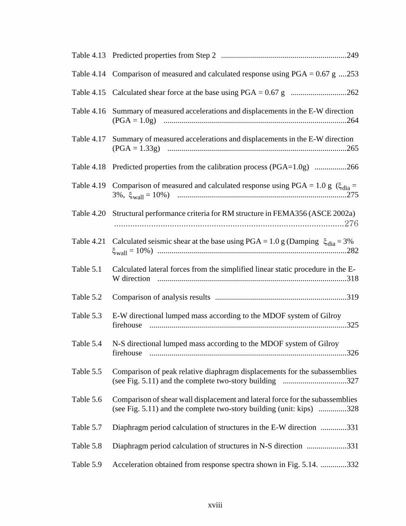
xviii

Table 4.13 Predicted properties from Step 2 ...............................................................249

Table 4.14 Comparison of measured and calculated response using PGA = 0.67 g ....253

Table 4.15 Calculated shear force at the base using PGA = 0.67 g ............................262

Table 4.16 Summary of measured accelerations and displacements in the E-W direction (PGA = 1.0g) ............................................................................................264

Table 4.17 Summary of measured accelerations and displacements in the E-W direction (PGA = 1.33g) ..........................................................................................265

Table 4.18 Predicted properties from the calibration process (PGA=1.0g) ................266

Table 4.19 Comparison of measured and calculated response using PGA = 1.0 g (ξdia = 3%, ξwall = 10%) .....................................................................................275

Table 4.20 Structural performance criteria for RM structure in FEMA356 (ASCE 2002a) ...................................................................................................276

Table 4.21 Calculated seismic shear at the base using PGA = 1.0 g (Damping ξdia = 3% ξwall = 10%) ...............................................................................................282

Table 5.1 Calculated lateral forces from the simplified linear static procedure in the E-W direction ...............................................................................................318

Table 5.2 Comparison of analysis results ..................................................................319

Table 5.3 E-W directional lumped mass according to the MDOF system of Gilroy firehouse ...................................................................................................325

Table 5.4 N-S directional lumped mass according to the MDOF system of Gilroy firehouse ...................................................................................................326

Table 5.5 Comparison of peak relative diaphragm displacements for the subassemblies (see Fig. 5.11) and the complete two-story building ................................327

Table 5.6 Comparison of shear wall displacement and lateral force for the subassemblies (see Fig. 5.11) and the complete two-story building (unit: kips) ..............328

Table 5.7 Diaphragm period calculation of structures in the E-W direction .............331

Table 5.8 Diaphragm period calculation of structures in N-S direction ....................331

Table 5.9 Acceleration obtained from response spectra shown in Fig. 5.14. .............332

xix

Table 5.10 Acceleration obtained from response spectra shown in Fig. 5.16. .............332

Table 5.11 Calculated lateral forces from the linear static procedure in -E-W direction .....................................................................................................................334

Table 5.12 Calculated lateral forces from the linear static procedure in N-S direction .....................................................................................................................335

Table 5.13 Comparison of in-plane wall lateral forces in the E-W direction .............336

Table 5.14 Comparison of in-plane wall lateral forces in N-S direction ....................340

Table 5.15 Comparison of displacement in the E-W direction ..................................344

Table 5.16 Comparison of displacement in N-S direction .........................................345

Table D.1 Outline UEL Input Variables ....................................................................404

xx

LIST OF FIGURES

Figure 1.1 Low-rise shear wall building with a nonrigid diaphragm: (a) Structural components and undeformed shape; (b) Bending mode in N-S direction; (c) Bending mode in E-W direction; (d) Shear raking mode in both direction; (e) Combined bending and shear raking modes in both directions. ...................10

Figure 1.2 Assembly of diaphragm and wall element DOFs to global DOFs. ..............11

Figure 1.3 Distributed Area and Lumped Mass Configuration. ....................................14

Figure 1.4 Inertial force of rigid and flexible diaphragm. .............................................17

Figure 1.5 Structural separation method for a story building with two flexible diaphragms. ..................................................................................................18

Figure 2.1 Analytical models: (a) Two DOFs model (Cohen 2000 a and b); (b) Lumped parameter model (Tena-Colunga and Abrams 1992a, 1992b, and 1996); (c) Equivalent frame model (Costley et al. 1996 and Kappos et al. 2002); and (d) Three-dimensional Finite Element Model (Tena-Colunga et al. 1992 and Kappos 2002). ...............................................................................................30

Figure 2.2 Plate girder under the horizontal loading. ....................................................33

Figure 2.3 (a) MDOF model of one bay one-story building with four in-plane shear walls, (b) Six degree-of-freedom diaphragm element. ...........................................35

Figure 2.4 (a) Mesh of diaphragm element showing 4 sampling points in each quadrant (b) General deformation of diaphragm element. ..........................................35

Figure 2.5 Independent displacement modes of a diaphragm element (three natural modes and three rigid body modes). .............................................................37

Figure 2.6 Calculation of the diaphragm deflection. .....................................................39

Figure 2.7 Internal stress distributions due to horizontal unit force, UN = 1. ................42

Figure 2.8 Example bending deflection due to chord splice slip. ........................45∆cs

xxi

Figure 2.9 Internal stress distributions due to vertical unit force, VN = 1. ...................46

Figure 2.10 Element shear raking mode and corresponding nodal forces. ......................47

Figure 2.11 Internal shear stress distribution in four quadrants of the diaphragm element for SN =1. ......................................................................................................48

Figure 2.12 Stresses and strains for each quadrant of a diaphragm. ...............................54

Figure 2.13 Stress-strain diagram example for each quadrant of a diaphragm. ..............55

Figure 2.14 Adjacent elements of diaphragm element. ...................................................57

Figure 2.15 (a) Typical cyclic force-deformation model (ABK 1981); (b) Diaphragm subjected to distributed loading; and (c) Diaphragm subjected to lumped loading. .........................................................................................................59

Figure 2.16 Typical cyclic load deflection model using three parameter model: (a) A trilinear representation and (b) Three parameter model (See Appendix A). .......................................................................................................................61

Figure 2.17 Specimen MAE-2. Load vs. displacement at loading points (Peralta et al. 2000). ............................................................................................................62

Figure 2.18 Experimental test and predicted force and displacement force and displacement relationship using three parameter model( , ,

and ). ..................................................................................................63

Figure 2.19 Force-deflection envelope of model (ABK 1981). .......................................65

Figure 2.20 Equivalent linear force-deformation model. .................................................66

Figure 2.21 Plywood sheathed diaphragm and load case. ..............................................70

Figure 2.22 Schematic layout for metal deck diaphragm. ...............................................80

Figure 2.23 Framing details and panel layout for a representative plywood diaphragm (Tissell and Elliott 1983). .............................................................................85

Figure 2.24 Example plywood diaphragm displacements. ..............................................87

Figure 2.25 Representative steel deck diaphragm (SDI 1995). .......................................89

Figure 2.26 Example steel deck diaphragm displacements. ............................................90

Figure 2.27 Comparison of deflection ratios. ..................................................................91

α 6.0= β 6.0=γ ∞=

xxii

Figure 2.28 Shear wall element: (a) single shear spring element and (b) multiple shear spring elements. ............................................................................................92

Figure 2.29 Compressive stress-strain response of masonry (MSJC 1999b). .................94

Figure 2.30 Example perforated wall (Schneider and Dickey 1994). ..............................96

Figure 2.31 Representation of a perforated cantilever wall (Tena-Colunga and Abrams 1992a). ........................................................................................................100

Figure 2.32 Calculation of story stiffness. .....................................................................101

Figure 2.33 Perforated walls for the comparison between the simplified and the FEM analysis. ......................................................................................................102

Figure 2.34 Diagonal tension cracking. .........................................................................106

Figure 2.35 Principal stress for unit area. ......................................................................107

Figure 2.36 Example of diagonal tension cracking response of simple piers (Magenes and Calvi 1997). ................................................................................................109

Figure 2.37 Bed joint sliding. ........................................................................................110

Figure 2.38 Bed joint sliding behavior (Shing 1998) and uniaxial bed-joint sliding hysteresis model. ........................................................................................111

Figure 2.39 Assumed effective shear zone and free body diagram of wall cracked at base .................................................................................................................... 113

Figure 2.40 Equilibrium of masonry pier. .....................................................................115

Figure 2.41 Load history for masonry wall test (Erbay and Abrams 2002) and the assumed uniaxial rocking hysteresis model. .............................................................117

Figure 2.42 Example of rocking response of simple piers (Magenes and Calvi 1997) .117

Figure 2.43 Assumed free body diagram of a two-story pier associated with a multiple-story rocking failure. ..................................................................................120

Figure 2.44 Assumed stress distribution at the interface between a lintel and a pier, based on an idealized flexural cracking model. ....................................................121

Figure 2.45 The procedure of calculating the elastic stiffness contribution of the each components of a perforated wall. ...............................................................124

xxiii

Figure 2.46 Three dimensional model with one diaphragm, four in-plane and one out-of-plane walls. .................................................................................................126

Figure 3.1 Firehouse at Gilroy, CA. ............................................................................133

Figure 3.2 Second floor plan. .......................................................................................133

Figure 3.3 South wall. ..................................................................................................134

Figure 3.4 East wall. ....................................................................................................134

Figure 3.5 Damage on the southeast corner of south wall. (Tena-Colunga and Abrams 1992a). ........................................................................................................135

Figure 3.6 Location of sensors at the firehouse at Gilroy. ...........................................136

Figure 3.7 N-S direction acceleration at the ground floor slab (U1), PGA = 0.24g at 5.2 sec. ........................................................................................................136

Figure 3.8 E-W direction acceleration at the ground floor slab (U3), PGA = 0.29g at 4.48 sec. ......................................................................................................137

Figure 3.9 E-W direction acceleration adjacent to the central wall (U4) .....................137

Figure 3.10 Three-dimensional analysis model of Gilroy firehouse. ............................138

Figure 3.11 Deformed shape and minimum in-plane principal stress plot for south wall. ................................................................................................................ 145

Figure 3.12 Deformed shape and minimum in-plane principal stress plot for central wall. .....................................................................................................................145

Figure 3.13 Deformed shape and minimum in-plane principal stress plot for north wall. .....................................................................................................................146

Figure 3.14 Deformed shape and minimum principal stress plot for east wall. ............146

Figure 3.15 Deformed shape and minimum principal stress plot for west wall. ...........147

Figure 3.16 Pier-type collapse mechanism. ...................................................................150

Figure 3.17 Multiple story type collapse mechanism. ...................................................150

Figure 3.18 Right side pier of the south wall. ................................................................152

Figure 3.19 Lumped mass ID at 2nd floor diaphragm. ..................................................160

xxiv

Figure 3.20 Lumped mass ID at roof diaphragm. ..........................................................161

Figure 3.21 Foundation load and Uncoupled Spring Model. .........................................164

Figure 3.22 SDOF model including soil-interaction effects and ground motions. ........164

Figure 3.23 (a) Undeformed three-dimensional model and (b) Key mode shapes of Gilroy Fire House. .................................................................................................167

Figure 3.24 Added shear spring model at roof diaphragm in the N-S direction. ...........169

Figure 3.25 Comparison of measured and computed displacement response of roof diaphragm displacement in the E-W direction (U5-U3). ............................171

Figure 3.26 Comparison of measured and computed displacement response of roof diaphragm displacement in the N-S direction (U6-U1). .............................172

Figure 3.27 Comparison of measured and computed displacement response of in-plane drift of interior wall at the roof level in the E-W direction (U4-U3). .........172

Figure 3.28 Comparison of measured and computed acceleration at the top of central wall in the E-W direction (U4). ..........................................................................172

Figure 3.29 Comparison of measured and computed acceleration at the center of south diaphragm in the E-W direction (U5). ........................................................173

Figure 3.30 Comparison of measured and computed acceleration at the center of south diaphragm in the N-S direction (U6). .........................................................173

Figure 3.31 Nonlinear time history response of the building using shear strength in Tables 3.8 through 3.12. .........................................................................................177

Figure 3.32 Nonlinear time history response of the building using updated strength shear strength. ......................................................................................................180

Figure 3.33 Displaced shape including both in-plane and out-of-plane wall deformations at 5.2 second during the time history analysis. ...........................................181

Figure 3.34 Comparison of wall force and displacement between the flexible (Get) and rigid diaphragm structure. ..........................................................................183

Figure 3.35 Comparison of in-plane shear forces using three different diaphragms: (a) first story and (b) second story. ..........................................................................184

Figure 3.36 Comparison of displacement response using three different diaphragm stiffnesses. ..................................................................................................186

xxv

Figure 4.1 Overall view of test building and nodal locations for the analytical model. ....................................................................................................................193

Figure 4.2 Overall photograph of specimen (Cohen 2001). ........................................193

Figure 4.3 Photograph of diaphragm showing the location of accelerometers (Cohen 2001). ..........................................................................................................195

Figure 4.4 Instrumentation for measuring horizontal accelerations and global point displacements at roof diaphragm. ...............................................................196

Figure 4.5 Damage to east and west walls from E-W shaking: (a) Photograph and (b) Idealized crack patterns of east and west walls (Cohen 2001). ..................196

Figure 4.6 Analytical model. .......................................................................................198

Figure 4.7 Node number and the associated degree-of-freedom of diaphragm element. ....................................................................................................................199

Figure 4.8 Photograph of diaphragm test setup (Cohen and Klingner 2001a). ...........201

Figure 4.9 Plan drawing of test set up for the diaphragm (Cohen and Klingner 2001a). ....................................................................................................................201

Figure 4.10 Typical cross-section of test setup at loading points (Cohen and Klingner 2001a). ........................................................................................................202

Figure 4.11 Relationship between applied load and diaphragm drift ratio for low diaphragm drift ratios (Tests #1 - #5) from the diaphragm test (Cohen and Klingner 2001a). .........................................................................................203

Figure 4.12 Relationship between applied load and diaphragm drift ratio for high diaphragm drift ratios from the diaphragm test (Tests #6 - #9) (Cohen and Klingner 2001a). .........................................................................................203

Figure 4.13 Comparison of measured and analysis model for low diaphragm drift ratios (Tests #1 - #5) from the diaphragm test. ....................................................204

Figure 4.14 Frictional force for low diaphragm from the diaphragm test (Tests #1 and #2). ....................................................................................................................205

Figure 4.15 Contribution of friction to hysteretic curve (Cohen and Klingner 2001a). 205

Figure 4.16 Comparison of measured and modified hysteretic curve in which frictional forces are extracted from measured forces for low diaphragm drift ratios (Tests #1 - #5). ............................................................................................206

xxvi

Figure 4.17 Comparison of measured and modified hysteretic curve in which frictional forces are extracted from measured forces for low diaphragm drift ratios (Tests #6 - #9). ............................................................................................207

Figure 4.18 Diaphragm analysis model associated with the modified hysteretic curve for Tests #1- #5. ...............................................................................................207

Figure 4.19 Diaphragm analysis model associated with the modified hysteretic curve for Tests #6- #9. ...............................................................................................208

Figure 4.20 Comparison of hysteresis envelopes. .........................................................208

Figure 4.21 Summary of hysteretic properties of three parameter model for diaphragm element: (a) Stiffness and strength, (b) Hysteresis model. .........................211

Figure 4.22 Reinforcement of masonry walls: (a) North and south wall; (b) East wall; (c) Plan; (d) North and south wall detail; and (e) East and west wall detail (Cohen 2001). ..........................................................................................................213

Figure 4.23 In-plane wall detailed section. ....................................................................217

Figure 4.24 Compressive area for out-of-plane masonry wall. .....................................218

Figure 4.25 Deformed shaped of the structure: (a) structure with rigid diaphragm, (b) structure with rigid diaphragm and east and west wall, and (c) structure with flexible diaphragm. .....................................................................................219

Figure 4.26 Shear and axial force contribution of out-of-plane walls. ..........................220

Figure 4.27 Instrument two corners and mid-frame in two directions for measuring horizontal acceleration at lifting frame. ......................................................223

Figure 4.28 Assembly of combined damping matrices. ................................................226

Figure 4.29 Eigenmode shapes of the building. ............................................................228

Figure 4.30 Variation of damping ratio and frequency for Rayleigh damping. ............228

Figure 4.31 Recorded relative displacement at the center of the diaphragm. ................231

Figure 4.32 Calculated relative displacement at the center of the diaphragm applying three measured acceleration at the lifting frame. .................................................231

Figure 4.33 1/2 second comparison of measured and calculated history varying time step from 0.005sec to 0.001sec. .........................................................................232

xxvii

Figure 4.34 Model calibration process used for wall properties. ...................................234

Figure 4.35 0.3 second comparisons of measured and calculated response (Damping: ξdia = 3%, ξwall = 3%). ......................................................................................240

Figure 4.36 Measured acceleration at the center of the diaphragm employed in the analysis with PGA =0.5g ..........................................................................................240

Figure 4.37 Calculated acceleration at the center of the diaphragm applying the average acceleration employed in the analysis with PGA =0.5g (Damping: ξdia = 3%, ξwall = 3%) ..................................................................................................241

Figure 4.38 Calculated acceleration at the center of the diaphragm applying the average acceleration employed in the analysis with PGA =0.5g (Damping: ξdia =3%, ξwall = 10%) ................................................................................................241

Figure 4.39 Two-second comparison of acceleration at the center of the diaphragm applying the average acceleration with PGA = 0.5g (Damping: ξdia = 3%, ξwall = 3%). .........................................................................................................241

Figure 4.40 Two-second comparison of acceleration at the center of the diaphragm applying the average acceleration with PGA = 0.5g (Damping: ξdia = 3%, ξwall = 10%) ........................................................................................................242

Figure 4.41 Measured displacement at the center of the diaphragm for Test 3 with PGA = 0.5g. ............................................................................................................242

Figure 4.42 Calculated displacement at the center of the diaphragm for Test 3 with PGA = 0.5g. (Damping: ξdia = 3%, ξwall = 3%) .....................................................242

Figure 4.43 Calculated displacement at the center of the diaphragm for Test 3 with PGA = 0.5g. (Damping: ξdia = 3%, ξwall = 10%). ..................................................243

Figure 4.44 Two-second comparison of displacement at the center of the diaphragm for Test 3 with PGA = 0.5g. (Damping: ξdia = 3%, ξwall = 3%) ......................243

Figure 4.45 Two-second comparison of displacement at the center of the diaphragm for Test 3 with PGA = 0.5g. (Damping: ξdia = 3%, ξwall = 10%) ....................243

Figure 4.46 Comparison of acceleration at the center of the diaphragm without the out-of-plane wall for PGA = 0.5g. (Damping: ξdia = 3%, ξwall = 3%) .................244

Figure 4.47 Two second comparison of acceleration at the center of the diaphragm without the out-of-plane wall for PGA = 0.5g. (Damping: ξdia = 3%, ξwall = 3%) ....................................................................................................................244

xxviii

Figure 4.48 Comparison of displacement at the center of the diaphragm without the out-of-plane wall for PGA = 0.5g. (Damping: ξdia = 3%, ξwall = 3%) .............245

Figure 4.49 Two second comparison of displacement at the center of the diaphragm without the out-of-plane wall for PGA = 0.5g. (Damping: ξdia = 3%, ξwall = 3%) .............................................................................................................245

Figure 4.50 0.15 second comparison of accelerations at the center of the diaphragm with changing Fs' in the bi-linear curve (K1 = 16kips/in, K2 = 9kips/in, Damping: ξdia = 3%, ξwall = 3%) ................................................................................251

Figure 4.51 0.15 second comparison of displacements at the center of the diaphragm with changing Fs' in the bi-linear curve (K1 = 16kips/in, K2 = 9kips/in, Damping: ξdia = 3%, ξwall = 3%) ...............................................................................251

Figure 4.52 The diaphragm response with changing the out-of-plane wall shear strengths (K1 = 16kips/in, K2 = 9kips/in, Damping: ξdia = 3%, ξwall = 3%). ...........252

Figure 4.53 Summary of Rayleigh damping coefficients. .............................................254

Figure 4.54 Comparison of the relative displacement at the center of the diaphragm varying the stiffness proportional damping of the out-of-plane wall: (a) a1=0.00097, (b) a1=0.00028, (c) a1=0.0001, (d) 0.3 second comparison. ..256

Figure 4.55 Comparison of the acceleration at the center of the diaphragm varying the stiffness proportional damping of the out-of-plane wall: (a) a1=0.00097, (b) a1=0.00028, (c) a1=0.0001, (d) 0.3 second comparison. ............................257

Figure 4.56 Comparison of the relative displacement at the top of the south wall varying the stiffness proportional damping of the out-of-plane wall: (a) a1=0.00097, (b) a1=0.00028, (c) a1=0.0001, (d) 0.5 second comparison. ......................258

Figure 4.57 Comparison of the acceleration at the top of the south wall varying the stiffness proportional damping of the out-of-plane wall: (a) a1=0.00097, (b) a1=0.00028, (c) a1=0.0001, (d) 0.2 second comparison. ............................259

Figure 4.58 Measured acceleration at the center of the diaphragm with PGA =0.67g (Damping: ξdia = 3%, ξwall = 3%) ..............................................................260

Figure 4.59 Calculated acceleration at the center of the diaphragm with PGA =0.67g (Damping: ξdia = 3%, ξwall = 3%) ..............................................................260

Figure 4.60 Two-second comparison of acceleration at the center of the diaphragm with PGA = 0.67g (Damping: ξdia = 3%, ξwall = 3%) ........................................260

xxix

Figure 4.61 Comparison of displacement at the center of the diaphragm with PGA = 0.67g (Damping: ξdia = 3%, ξwall = 3%) ..............................................................261

Figure 4.62 Comparison of displacement at the center of the diaphragm with PGA = 0.67g (Damping: ξdia = 3%, ξwall = 3%) ..............................................................261

Figure 4.63 Two-second comparison of displacement at the center of the diaphragm applying the average acceleration employed in the analysis for PGA = 0 67g (Damping: ξdia = 3%, ξwall = 3%) ..............................................................261

Figure 4.64 Comparison of relative displacement at the top of south wall using three different in-plane wall damping ratio: (a) 10% damping; (b) 5% damping; (c) 3% damping; and (d) 0.2 sec comparison of three different damping. ......268

Figure 4.65 Comparison of relative displacement at the center of diaphragm using three different in-plane wall damping ratio: (a) 10% damping; (b) 5% damping; (c) 3% damping; and (d) 0.2 sec comparison of three different damping. ......269

Figure 4.66 In-plane south wall hysteresis curve employed in the analysis for PGA = 1.0g (Damping: ξdia = 3%, ξwall = 10%). ...........................................................271

Figure 4.67 In-plane north wall hysteresis curve employed in the analysis for PGA = 1 0g (Damping: ξdia = 3%, ξwall = 10%). ...........................................................271

Figure 4.68 Comparison of force and displacement at the south wall using three different in-plane wall strength: (a) Fy = infinite; (b) Fy = 2.0 kips; (c) Fy = 1.75 kips; and (d) 0.2 sec comparison of three different strength. (Damping: ξdia = 3%, ξwall = 10%) ................................................................................................272

Figure 4.69 Out-of-plane wall hysteresis curve employed in the analysis for PGA = 1 0g (Damping: ξdia = 3%, ξwall = 10%) ............................................................273

Figure 4.70 Diaphragm Hysteresis curve employed in the analysis for PGA = 1.0g (Damping: ξdia = 3%, ξwall = 10%) ............................................................274

Figure 4.71 Measured displacement at the top of south wall with PGA = 1.0g (Damping: ξdia = 3%, ξwall = 10%) ..............................................................................277

Figure 4.72 Calculated displacement at the top of south wall with PGA = 1.0g (Damping: ξdia = 3%, ξwall = 10%) ..............................................................................277

Figure 4.73 Two-second comparison of displacement at the top of south wall with PGA =1.0g (Damping: ξdia = 3%, ξwall = 10%) ..................................................277

Figure 4.74 Measured acceleration at the top of south wall with PGA = 1.0g (Damping: ξdia = 3%, ξwall = 10%) ..............................................................................278

xxx

Figure 4.75 Calculated acceleration at the top of south wall with PGA = 1.0g (Damping: ξdia = 3%, ξwall = 10%) ..............................................................................278

Figure 4.76 Two-second comparison of acceleration at the top of south wall with PGA =1.0g (Damping: ξdia = 3%, ξwall = 10%) ..................................................278

Figure 4.77 Measured displacement at the center of the diaphragm with PGA = 1.0g (Damping: ξdia = 3%, ξwall = 10%) ............................................................279

Figure 4.78 Calculated displacement at the center of the diaphragm with PGA = 1.0g (Damping: ξdia = 3%, ξwall = 10%) ............................................................279

Figure 4.79 Two-second comparison of displacement at the center of the diaphragm with PGA = 1.0g (Damping: ξdia = 3%, ξwall = 10%) ........................................279

Figure 4.80 Measured acceleration at the center of the diaphragm with PGA = 1.0g (Damping: ξdia = 3%, ξwall = 10%) ............................................................280

Figure 4.81 Calculated acceleration at the center of the diaphragm with PGA = 1.0g (Damping: ξdia = 3%, ξwall = 10%) ............................................................280

Figure 4.82 Two-second comparison of acceleration at the center of the diaphragm with PGA = 1.0g (Damping: ξdia = 3%, ξwall = 10%) ........................................280

Figure 4.83 Measured acceleration at the center of the diaphragm with PGA = 1.33g (Damping: ξdia = 3%, ξwall = 10%) ............................................................281

Figure 4.84 Calculated acceleration at the center of the diaphragm with PGA = 1.33g (Damping: ξdia = 3%, ξwall = 10%) ............................................................281

Figure 4.85 Two-second comparison of acceleration at the center of the diaphragm with PGA = 1.33g (Damping: ξdia = 3%, ξwall = 10%) ......................................281

Figure 4.86 Variation of the diaphragm backbone curves corresponding to (a) the decreased initial stiffnesses and (b) the increased initial stiffnesses ..........285

Figure 4.87 Variation of the in-plane wall backbone curves corresponding to the increased initial stiffnesses and strength. ...................................................................286

Figure 4.88 Variation of the out-of-plane wall backbone curves corresponding to the increased initial stiffnesses and strength ....................................................286

Figure 4.89 Peak out-of-plane wall drift ratio varying the diaphragm stiffness from Kd/Kd* = 0.4 (flexible diaphragm) to 40 (rigid diaphragm) ...................................287

xxxi

Figure 4.90 (a) Peak out-of-plane wall drift ratio varying the diaphragm stiffness from Kd/Kd* = 0.4 (very flexible diaphragm) to 5 (flexible diaphragm), (b) Hysteretic curves of structural components for Kd/Kd* = 0.7; (c) for Kd/Kd* = 2; and (d) for Kd/Kd* = 2.9. ........................................................................................288

Figure 4.91 Peak in-plane wall drift ratio varying the diaphragm stiffness from Kd/Kd* = 0.4 (flexible diaphragm) to 40 (rigid diaphragm) .......................................289

Figure 4.92 (a) Peak in-plane wall drift ratio varying the diaphragm stiffness from Kd/Kd* = 0.4 (very flexible diaphragm) to 6 (flexible diaphragm) (b) Hysteretic curves of structural components for Kd/Kd* = 2; (c) for Kd/Kd* = 2.9; and (d) for Kd/Kd* = 5.7. ...................................................................................................290

Figure 4.93 Peak acceleration at diaphragm varying the diaphragm stiffness from Kd/Kd* = 0.4 (flexible diaphragm) to 40 (rigid diaphragm) ...................................291

Figure 4.94 Peak acceleration at diaphragm varying the diaphragm stiffness from Kd/Kd* = 0.4 (very flexible diaphragm) to 5 (flexible diaphragm) .........................291

Figure 4.95 Displacement response spectrum of time-scaled (factor = 0.5) input record used for ground excitation ..........................................................................292

Figure 4.96 Peak out-of-plane wall drift ratio varying the in-plane wall stiffness from Kip/Kip* = 0.33 to 4. ...................................................................................293

Figure 4.97 Peak in-plane wall drift ratio varying the in-plane wall stiffness from Kip/Kip* = 0.33 to 4. ..................................................................................................293

Figure 4.98 Peak acceleration at diaphragm varying the in-plane wall stiffness from Kip/Kip* = 0.33 to 4. ...................................................................................294

Figure 4.99 Peak out-of-plane wall drift ratio varying the out-of-plane wall stiffness from Kop/Kop* = 0 (neglecting out-of-plane wall) to 3. .....................................295

Figure 4.100 Peak in-plane wall drift ratio varying the out-of-plane wall stiffness from Kop/Kop* = 0 (neglecting out-of-plane wall) to 3. .....................................295

Figure 4.101 Peak acceleration at diaphragm varying the out-of-plane wall stiffness from Kop/Kop* = 0 (neglecting out-of-plane wall) to 3. .....................................296

Figure 5.1 Simplified procedure for low-rise building with flexible diaphragms. ......305

Figure 5.2 Base shear calculation for the MDOF system of a one-story building with a flexible diaphragm and out-of-plane walls: (a) MDOF system; (b) Acceleration and inertial forces; (c) Diaphragm load distribution to in-plane and out-of-plane walls, and (d) Approximate calculation of reactions. .....306

xxxii

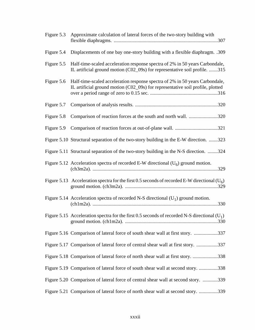
Figure 5.3 Approximate calculation of lateral forces of the two-story building with flexible diaphragms. ...................................................................................307

Figure 5.4 Displacements of one bay one-story building with a flexible diaphragm. .309

Figure 5.5 Half-time-scaled acceleration response spectra of 2% in 50 years Carbondale, IL artificial ground motion (C02_09s) for representative soil profile. .......315

Figure 5.6 Half-time-scaled acceleration response spectra of 2% in 50 years Carbondale, IL artificial ground motion (C02_09s) for representative soil profile, plotted over a period range of zero to 0.15 sec. ......................................................316

Figure 5.7 Comparison of analysis results. ..................................................................320

Figure 5.8 Comparison of reaction forces at the south and north wall. .......................320

Figure 5.9 Comparison of reaction forces at out-of-plane wall. ..................................321

Figure 5.10 Structural separation of the two-story building in the E-W direction. .......323

Figure 5.11 Structural separation of the two-story building in the N-S direction. ........324

Figure 5.12 Acceleration spectra of recorded E-W directional (U6) ground motion. (ch3m2a). ....................................................................................................329

Figure 5.13 Acceleration spectra for the first 0.5 seconds of recorded E-W directional (U6) ground motion. (ch3m2a). ..........................................................................329

Figure 5.14 Acceleration spectra of recorded N-S directional (U1) ground motion. (ch1m2a). ....................................................................................................330

Figure 5.15 Acceleration spectra for the first 0.5 seconds of recorded N-S directional (U1) ground motion. (ch1m2a). ..........................................................................330

Figure 5.16 Comparison of lateral force of south shear wall at first story. ...................337

Figure 5.17 Comparison of lateral force of central shear wall at first story. .................337

Figure 5.18 Comparison of lateral force of north shear wall at first story. ....................338

Figure 5.19 Comparison of lateral force of south shear wall at second story. ...............338

Figure 5.20 Comparison of lateral force of central shear wall at second story. ............339

Figure 5.21 Comparison of lateral force of north shear wall at second story. ...............339

xxxiii

Figure 5.22 Comparison of lateral forces in the E-W direction. ....................................340

Figure 5.23 Comparison of lateral force of east shear wall at first story. ......................341

Figure 5.24 Comparison of lateral force of west shear wall at first story. .....................341

Figure 5.25 Comparison of lateral force of east shear wall at second story. .................342

Figure 5.26 Comparison of lateral force of west shear wall at second story. ................342

Figure 5.27 Comparison of lateral forces in N-S direction. ...........................................343

Figure A.1 Parameter. ..............................................................................................358

Figure A.2 Parameter. ...............................................................................................359

Figure A.3 Parameter. ..............................................................................................360

Figure A.4 Hysteresis rules. ..........................................................................................361

Figure B.1 Diaphragm layout of Roof Level. ...............................................................362

Figure B.2 Diaphragm layout of 2nd Floor Level. .......................................................363

Figure B.3 South Wall, Firehouse of Gilroy. ...............................................................364

Figure B.4 Central Wall, Firehouse of Gilroy. .............................................................365

Figure B.5 North Wall, Firehouse of Gilroy. ...............................................................366

Figure B.6 East Wall, Firehouse of Gilroy. ..................................................................367

Figure B.7 West Wall, Firehouse of Gilroy. .................................................................368

Figure B.8 Piers of south wall using the pier-type collapse mechanism. .....................369

Figure B.9 Piers of central wall using the pier-type collapse mechanism. ...................369

Figure B.10 Piers of north wall using the pier-type collapse mechanism. .....................370

Figure B.11 piers of east wall using the pier-type collapse mechanism. ........................370

Figure B.12 Piers of west wall using the pier-type collapse mechanism. ......................371

Figure C.1 Plan of Test Building. .................................................................................372

α

β

γ

xxxiv

Figure C.2 East Wall of Test Building. ........................................................................372

Figure C.3 West Wall of Test Building. .......................................................................373

Figure C.4 North and South Wall of Test Building. .....................................................373

Figure C.5 Measured accelerations in the E-W direction at lifting frame (Specimen #1 Test 3) (Cohen 2001). .................................................................................374

Figure C.6 One-second comparisons of measured accelerations in the E-W direction at lifting frame (Specimen #1 Test 3) (Cohen 2001). .....................................374

Figure C.7 Comparison of measured accelerations in the E-W direction at the center of diaphragm and the top of the north and south wall (Specimen #1 Test 3) (Cohen 2001). .............................................................................................375

Figure C.8 One-second comparison of measured accelerations in the E-W direction at the center of diaphragm and the top of the north and south wall (Specimen #1 Test 3) (Cohen 2001). .........................................................................................375

Figure C.9 Comparison of measured accelerations in the E-W direction at the top of the south wall (Specimen #1 Test 3) (Cohen 2001). ........................................375

Figure C.10 One-second comparison of measured accelerations in the E-W direction at the top of the south wall (Specimen #1 Test 3) (Cohen 2001). .......................376

Figure C.11 Measured accelerations in the E-W direction at the top of the north wall (Specimen #1 Test 3) (Cohen 2001). ..........................................................376

Figure C.12 One-second comparison of measured accelerations in the E-W direction at the top of the north wall (Specimen #1 Test 3) (Cohen 2001). .......................376

Figure C.13 One-second comparison of measured displacements in the E-W direction (Specimen #1 Test 3) (Cohen 2001). ..........................................................377

Figure C.14 One-second comparison of measured displacements in the E-W direction (Specimen #1 Test 3) (Cohen 2001). ..........................................................377

Figure C.15 Comparison of measured displacements in the E-W direction at the top of the north and south wall (Specimen #1 Test 3) (Cohen 2001). ........................377

Figure C.16 One-second comparison of measured displacements in the E-W direction at the top of the north and south wall (Specimen #1 Test 3) (Cohen 2001). ..378

Figure C.17 Measured acceleration in the N-S direction at lifting frame (Specimen #1 Test 5) (Cohen 2001). .........................................................................................378

xxxv

Figure C.18 One-second comparison of measured acceleration in the N-S direction at lifting frame (Specimen #1 Test 5) (Cohen 2001). .....................................379

Figure C.19 Measured acceleration in the E-W direction at lifting frame (Specimen #1 Test 5) (Cohen 2001). .........................................................................................379

Figure C.20 One-second comparison of measured acceleration in the E-W direction at lifting frame (Specimen #1 Test 5) (Cohen 2001). .....................................379

Figure C.21 Comparison of measured accelerations in the E-W direction at diaphragm (Specimen #1 Test 5) (Cohen 2001). ..........................................................380

Figure C.22 One-second comparison measured accelerations in the E-W direction at diaphragm (Specimen #1 Test 5) (Cohen 2001). ........................................380

Figure C.23 Measured accelerations in the E-W direction at the top of south wall (Specimen #1 Test 5) (Cohen 2001). ..........................................................380

Figure C.24 One-second comparison of measured accelerations in the E-W direction at the top of south wall (Specimen #1 Test 5) (Cohen 2001). ..............................381

Figure C.25 Measured accelerations in the E-W direction at the top of north wall (Specimen #1 Test 5) (Cohen 2001). ..........................................................381

Figure C.26 One-second comparison of measured accelerations in the E-W direction at the top of north wall (Specimen #1 Test 5) (Cohen 2001). ..............................381

Figure C.27 Measured displacements in the E-W direction (Specimen #1 Test 5) (Cohen 2001). ..........................................................................................................382

Figure C.28 One-second comparison of measured displacements in the E-W direction (Specimen #1 Test 5) (Cohen 2001). ..........................................................382

Figure C.29 Measured displacements in the E-W direction at the top of the north and south wall (Specimen #1 Test 5) (Cohen 2001). ..................................................382

Figure C.30 One-second comparison of measured displacements in the E-W direction at the top of the north and south wall (Specimen #1 Test 5) (Cohen 2001). ..383

Figure C.31 Measured accelerations in the E-W direction at lifting frame (Specimen #1 Test 9) (Cohen 2001). .................................................................................383

Figure C.32 One-second comparisons of measured accelerations in the E-W direction at lifting frame (Specimen #1 Test 9) (Cohen 2001). .....................................384

xxxvi

Figure C.33 Comparison of measured accelerations in the E-W direction at the center of diaphragm and the top of the north and south wall (Specimen #1 Test 9) (Cohen 2001). .............................................................................................384

Figure C.34 One-second comparison of measured accelerations in the E-W direction at the center of diaphragm and the top of the north and south wall (Specimen #1 Test 9) (Cohen 2001). .........................................................................................384

Figure C.35 Comparison of measured accelerations in the E-W direction at the top of north and south wall (Specimen #1 Test 9) (Cohen 2001). .................................385

Figure C.36 One-second comparison of measured accelerations in the E-W direction at the top of north and south wall (Specimen #1 Test 9) (Cohen 2001). .............385

Figure C.37 Comparison of measured accelerations in the E-W direction at the top of south wall (Specimen #1 Test 9) (Cohen 2001). ..................................................385

Figure C.38 One-second comparison of measured accelerations in the E-W direction at the top of south wall (Specimen #1 Test 9) (Cohen 2001). ..............................386

Figure C.39 Comparison of measured accelerations in the E-W direction at the top of north wall (Specimen #1 Test 9) (Cohen 2001). ..................................................386

Figure C.40 One-second comparison of measured accelerations in the E-W direction at the top of north wall (Specimen #1 Test 9) (Cohen 2001). ..............................386

Figure C.41 Measured displacements in the E-W direction (Specimen #1 Test 9) (Cohen 2001). ..........................................................................................................387

Figure C.42 One-second comparison of measured displacements in the E-W direction (Specimen #1 Test 9) (Cohen 2001). ..........................................................387

Figure C.43 Measured displacements in the E-W direction at the top of the north and south wall (Specimen #1 Test 9) (Cohen 2001). ..................................................387

Figure C.44 One-second comparison of measured displacements in the E-W direction at the top of the north and south wall (Specimen #1 Test 9)(Cohen 2001). ...388

Figure C.45 Comparison of acceleration in the E-W direction at the top of south wall (PGA =0.5g). ........................................................................................................388

Figure C.46 Two-second comparison of acceleration in the E-W direction at the top of south wall (PGA =0.5g). .............................................................................389

Figure C.47 Comparison of acceleration in the E-W direction at the top of north wall (PGA =0.5g). ........................................................................................................389

xxxvii

Figure C.48 Two-second comparison of acceleration in the E-W direction at the top of north wall (PGA =0.5g). .............................................................................389

Figure C.49 Comparison of displacement in the E-W direction at the top of south wall (PGA =0.5g). ..............................................................................................390

Figure C.50 Two-second comparison of displacement in the E-W direction at the top of south wall (PGA =0.5g). .............................................................................390

Figure C.51 Comparison of displacement in the E-W direction at the top of north wall (PGA =0.5g). ..............................................................................................390

Figure C.52 Two-second comparison of displacement in the E-W direction at the top of north wall (PGA =0.5g). .............................................................................391

Figure C.53 Comparison of acceleration in the E-W direction at the top of south wall (PGA =0.67g). ......................................................................................................391

Figure C.54 Two-second comparison of acceleration in the E-W direction at the top of south wall (PGA =0. 67g). ..........................................................................392

Figure C.55 Comparison of acceleration in the E-W direction at the top of north wall (PGA =0. 67g). .....................................................................................................392

Figure C.56 Two-second comparison of acceleration in the E-W direction at the top of north wall (PGA =0.67g). ...........................................................................392

Figure C.57 Comparison of displacement in the E-W direction at the top of south wall (PGA =0. 67g). ...........................................................................................393

Figure C.58 Two-second comparison of displacement in the E-W direction at the top of south wall (PGA =0. 67g). ..........................................................................393

Figure C.59 Comparison of displacement in the E-W direction at the top of north wall (PGA =0. 67g). ...........................................................................................393

Figure C.60 Two-second comparison of displacement in the E-W direction at the top of north wall (PGA =0. 67g). ..........................................................................394

Figure C.61 Comparison of acceleration in the E-W direction at the top of south wall (PGA =1.0g). ........................................................................................................394

Figure C.62 Two-second comparison of acceleration in the E-W direction at the top of south wall (PGA = 1.0g). ............................................................................395

xxxviii

Figure C.63 Comparison of acceleration in the E-W direction at the top of north wall (PGA = 1.0g). .......................................................................................................395

Figure C.64 Two-second comparison of acceleration in the E-W direction at the top of north wall (PGA = 1.0g). ............................................................................395

Figure C.65 Comparison of displacement in the E-W direction at the top of south wall (PGA = 1.0g). .............................................................................................396

Figure C.66 Two-second comparison of displacement in the E-W direction at the top of south wall (PGA = 1.0g). ............................................................................396

Figure C.67 Comparison of displacement in the E-W direction at the top of north wall (PGA = 1.0g). .............................................................................................396

Figure C.68 Two-second comparison of displacement in the E-W direction at the top of north wall (PGA = 1.0g). ............................................................................397

Figure D.1 General ABAQUS Implementation Concepts. ...........................................399

Figure D.2 A schematic modeling of an arbitrary structure. ........................................399

Figure D.3 Overall Dataflow. .......................................................................................406

Figure D.4 Main Program. ............................................................................................407

1

CHAPTER I

INTRODUCTION

Masonry is a widely used material for building construction because of its versatil-

ity and appearance. According to Shing (1998), approximately 70 percent of the building

inventory in the United States employs masonry walls in some capacity as lateral-load

resisting elements. French and Olshansky (2000) categorize 33 percent of the essential

facilities within a study area of the New Madrid fault zone as unreinforced masonry

(URM), while eight percent of the essential facilities within this area are categorized in

their research as reinforced masonry. On this basis, an early decision of the Mid-America

Earthquake (MAE) Center Essential Facilities Program was to focus on masonry building

construction, particularly unreinforced masonry. The MAE Center was formed in the fall

of 1997 with the goal of helping to reduce significant economic losses that are expected

with a future earthquake in Mid-America. The purpose of the specific research addressed

in this dissertation is to develop and apply simplified analytical models for seismic assess-

ment of low-rise buildings with nonrigid floor and/or roof diaphragms. A key focus of this

work is on the modeling of low-rise masonry buildings. However, the approaches investi-

gated have some potential for other low-rise building types as well.

1.1 Research Objectives

In prior research, numerous approaches have been employed for analysis of the

dynamic response of low-rise shear wall building structures. These approaches range from

2

refined finite element models of the in-plane behavior of individual walls and diaphragms

to various types of coarse "lumped parameter" (or "discrete element") models. Many of

the three dimensional building analysis models have focused primarily on elastic, or lin-

earized, building responses.

The primary objectives of this research are:

1. To develop, test and validate a simplified three-dimensional linear and nonlinear mul-

tiple degree-of-freedom (MDOF) analysis approach for low-rise buildings (e.g., up to

four stories) with nonrigid diaphragms, and

2. To develop associated guidelines for linear static seismic evaluation of flexible dia-

phragm structures (i.e., buildings in which the diaphragm stiffness is small enough

such that torsional coupling effects can be neglected).

The following essential response characteristics are addressed:

• Diaphragm flexibility and nonlinear hysteretic response.

• Wall in-plane hysteretic response.

• Out-of-plane displacement of walls due to diaphragm flexibility.

• Stiffness, and strength associated with flange effects from out-of-plane walls.

• Influence of diaphragm response on the distribution of lateral forces to the structural

walls.

• Influence of diaphragm response on torsional coupling between the structural walls.

With respect to the first objective, emphasis is placed on capture of the three-dimensional

response as well the effects of potential significant nonlinearities using a small number of

degrees of freedom. It is intended for the methodologies developed in this research to be

useful for on-going and potential future studies pertaining to:

3

1. Reliable and rapid evaluation of the seismic vulnerability of specific buildings,

2. Analysis of the influence of nonrigid diaphragms on the response of low-rise masonry

buildings in general, and

3. Development of comprehensive guidelines for seismic evaluation of buildings with

nonrigid diaphragms.

1.2 Background and Problem Statement

There is a dearth of experimental and analytical work on the seismic performance

of low-rise buildings with nonrigid diaphragms. The lack of information on the dynamic

characteristics of nonrigid diaphragms and their influence on the seismic response of low-

rise buildings is evidenced in a lack of comprehensive guidance for seismic assessment of

these types of structures in FEMA 273 (FEMA 1997) and 356 (ASCE 2000a). This sec-

tion summarizes some of the research needs with respect to development of analysis mod-

els and with respect to seismic assessment of the above types of structures.

1.2.1 Research needs with respect to development of analysis models

Key structural components in the simplified analysis approach addressed in this

work are the shear walls and diaphragms. In masonry buildings, wall hysteretic models

should incorporate the effects of pier rocking, bed-joint sliding, toe crushing and diagonal

tension failure. Diaphragm hysteretic models should account for stiffness degradation,

strength deterioration and pinching characteristics in diaphragms. A detailed literature

review is outlined in Chapter 2. A few key previous studies are summarized below.

Flexible diaphragms have been idealized as beams by Shepherd and Donald

(1967), Lee and Moon (1989), Dolce et al. (1994), and Masi et al. (1997). Dolce et al.

4

(1994) idealized the floor diaphragm as a beam with its own elastic and elasto-plastic hys-

teresis curve. Masi et al. (1997) investigated the seismic response of irregular multi-story

reinforced concrete buildings with flexible inelastic diaphragms. The vertical elements

were idealized as shear springs and the diaphragm elements were idealized as beams.

Both the beam and spring elements had a capability to represent stiffness degradation.

Rutenberg (1980) used a deep-beam idealization to investigate laterally-loaded

flexible-diaphragm buildings. Kunnath et al. (1990, 1991, 1994) developed a special-pur-

pose hysteresis model to study the behavior of inelastic flexible concrete floor dia-

phragms. Kunnath’s idealization is based on beam theory. Tena-Colunga and Abrams

(1992a, 1992b, and 1996) used shear springs to model flexible diaphragms in two-dimen-

sional analyses. Beam models may be suitable for long narrow buildings with nonrigid

diaphragms (Jain and Jennings 1985 and Button et al. 1984). However the above types of

beam models do not consider explicitly the various three-dimensional effects (bending in

two orthogonal directions and overall raking of the diaphragms as “shear panels” between

the walls). These effects may have a significant influence on buildings with nonrigid dia-

phragms with small to moderate aspect ratios in plan.

A finite element model that predicts the cyclic in-plane behavior of slabs was for-

mulated by Chen (1986). Refined finite elements were also used to model floor slabs by

Saffarini and Qudaimat (1992), Lopez et al. (1994), and Costley and Abrams (1996).

Kunnath et al. (1991) found that the element developed by Chen could not be readily

applied to an entire building. Costley and Abrams (1996) suggested that there is a need

for improved simplified models for estimating response maxima of URM buildings with

flexible diaphragms.

The number of degrees of freedom in the analytical model of low-rise buildings

with nonrigid diaphragms should be kept small for efficiency in rapid evaluation of physi-

cal buildings or test designs, as well as in conducting large numbers of analyses in simula-

tion studies of low-rise shear wall buildings with nonrigid diaphragms.

5

1.2.2 Research needs in seismic assessment

The FEMA 357 Global Topics Report on The Prestandard and Commentary for

The Seismic Rehabilitation of Buildings (ASCE 2000b), outlines several issues in which

research on the inelastic performance of the buildings with nonrigid diaphragm is needed.

A few of the needs, which are still largely unresolved in 2002, are:

• “Some building types, such as URM or tilt-up structures, may be more appropriately

evaluated as systems rather than components. Flexible wood diaphragms in rigid wall

buildings may need special treatment…. The response amplification of ground motion

occurs in the diaphragm of rigid wall flexible diaphragm systems. As such, the behav-

ior of individual components such as wall anchors depends on the overall system

behavior” (Global Issues 3-8 in FEMA 357, ASCE 2000b).

• “The definition of torsion and the procedure for amplification of torsion need further

clarification. … The current definition does not discuss dynamic torsion, or torsion

due to rotational modes of building response. This is a dynamic characteristic of the

system that may produce torsion in excess of that due to eccentricity between the cen-

ter of mass and center of rigidity. Currently the Guidelines only require accidental tor-

sion to be amplified” (Global Issues 3-22 in FEMA 357, ASCE 2000b).

• “Procedures for torsional amplification do not account for torsional degradation and

are not conservative in determining increased forces and displacements for this effect.

… Reportedly there have been recent studies in Japan indicating that further amplifi-

cation of forces and displacements is required to properly account for torsion as the

stiffness of the structure degrades in the direction perpendicular to the direction under

consideration” (Global Issues 3-38 in FEMA 357, ASCE 2000b).

• “Further guidance is required on the proper application of the NSP [Nonlinear Static

Procedure] in buildings with nonrigid diaphragms. … In buildings with nonrigid dia-

6

phragms, some of the deformation demand can be taken up in diaphragm deflection.

This could be unconservative in estimating deformation demands on vertical seismic

framing elements. To approximately account for this, FEMA 273 included provisions

for amplifying the calculated target displacement by the ratio of the maximum dia-

phragm displacement to the displacement at the center of mass. However, pushing the

vertical elements to the full target without consideration of diaphragm deflections is

overconservative. Development of methods to explicitly apply the NSP to nonrigid

diaphragms is recommended….” (Global Issues 3-36 in FEMA 357, ASCE 2000b).

There is little information on the three-dimensional behavior of shear wall build-

ings with nonrigid diaphragms (Abrams 2001). Although there have been several experi-

mental tests of low-rise shear wall buildings with flexible diaphragms, many questions

remain regarding the behavior and analysis of these types of buildings. No attempt has

been made to perform extensive numerical studies of the three-dimensional inelastic

response of these types of structures.

1.3 Contributions of this research

This research addresses the development of simplified methods of analysis and

seismic assessment for shear wall type building structures with nonrigid diaphragms.

The work focuses on low-rise wall-type buildings with rectangular plan geometry.

A three-dimensional linear and nonlinear analysis approach is created to allow for accu-

rate and rapid seismic assessment for these types of buildings. The suggested approach is

efficient enough for the rapid evaluation of physical buildings or test designs, and for con-

ducting large numbers of analyses within simulation studies. The approach utilizes new

diaphragm and wall elements developed in this research. The diaphragm element is based

on a flexibility (equilibrium) based formulation to calculate its stiffness and overall non-

linear force deformation response. Strength and hysteretic properties of the diaphragm

7

element are estimated from the results of experimental tests conducted in previous

research. The wall element involves a simple shear spring idealization. In order to most

accurately estimate the initial stiffness coefficients of shear walls, a flexibility approach is

recommended using the results of plane stress finite element analysis. Simple equations

based on mechanics of materials are also considered for calibration of the wall stiffnesses.

As noted at the beginning of this chapter, unreinforced masonry is a major con-

struction material in existing essential facilities in mid America. Thus, an early decision

of this research was to focus on the nonlinear characteristics of these types of buildings.

The hysteretic properties of the structural components of these buildings are approximated

in this work based on previous experimental tests. The wall and diaphragm elements are

implemented with computer graphics visualization, as a post-processing tool, to manage

the massive analysis outputs for better understating of the behavior of these buildings.

The MDOF model discussed above can be used for simplified three-dimensional

nonlinear time history analysis of low-rise shear wall rectangular building structures.

Comparisons of analytical studies to experimental tests can be valuable for understanding

the seismic response of these types of buildings and for determining the qualities and lim-

itations of simplified models. To this end, the proposed simplified MDOF analysis

approach is applied to a two-story unreinforced masonry historic building with interior

walls and multiple diaphragms in each story, and to a half-scale single-story reinforced

masonry test building with a single diagonally-sheathed diaphragm. The two-story build-

ing was instrumented within the California Strong Motion Instrumentation Program

(CSMIP) and withstood the Loma Prieta earthquake in 1989. This building, which is

referred to as the Gilroy Firehouse, was previously studied extensively by Tena-Colunga

and Abrams (1992). The single-story building was constructed and tested on the shaking

table at the United States Army Construction Engineering Research Laboratory (CERL),

and was subsequently studied by Cohen (2002a). The structural properties of the Gilroy

Firehouse are calculated based on extensions to various current methods prescribed in

8

FEMA 273 (FEMA 1997) and 356 (ASCE 2002a) as well as other publications and devel-

opments from this research. The structure is analyzed based on these properties, and

modifications necessary to obtain improved predictions relative to the field test data are

discussed. For the single story test building, a model calibration process is performed in

this work to determine the required structural properties based on the elastic and inelastic

test responses. This approach is necessary since it is difficult to determine accurately the

in-plane and out-of-plane stiffness, strength, and hysteresis using simplified equations

specified in current seismic codes and standards. The comparison between the structural

properties obtained by this calibration process and by various simple strength of materials

type procedures are discussed.

Lastly, a simplified linear static procedure is proposed for low-rise buildings with

flexible diaphragms. This method involves the consideration of the individual diaphragms

and the associated out-of-plane walls within a building via separate idealized single

degree of freedom models. The shear forces calculated from the separated models are

combined to obtain wall shear forces. The final forces and displacements determined

using this simplified linear static procedure are compared with linear time history analysis

results for the one- and two-story buildings discussed in this research, and conclusions

regarding the use of this approach are discussed.

1.4 Overview of proposed simplified three-dimensional MDOF analysis approach

In the three-dimensional analysis approaches developed in this work, a building

subdivided into its horizontal roof or floor diaphragms and their supporting vertical ele-

ments as shown in Fig. 1.1. This figure illustrates the general deformation of buildings

with nonrigid diaphragms. These figures show the three key idealized modes of dia-

phragm displacement: an out-of-plane bending mode in the N-S direction (Fig. 1.1(b)); an

out-of-plane bending mode in the E-W direction (Fig. 1.1(c)); and a shear raking mode

9

(Fig. 1.1(d)). The distribution of the horizontal forces to the vertical elements depends on

the geometry and the rigidity of the nonrigid diaphragm. Floor diaphragms can be classi-

fied as flexible, stiff and rigid (ASCE 2000a). The prediction of the behavior of a struc-

ture with rigid diaphragm is relatively easy compared to that of structures with nonrigid

diaphragm because the three key modes of diaphragm deformation shown in Fig. 1.1 do

not exist in this case.

As the rigid diaphragm does not deform appreciably, it is assumed that its behavior

remains elastic and the earthquake-induced internal forces are generally distributed to the

vertical resisting elements in direct proportion to the relative rigidities of these elements.

Conversely, in nonrigid diaphragm structures, the horizontal force within the vertical ele-

ments due to the lateral excitation depends on the rigidity and strength of the diaphragms.

In this section, the essential components that comprise the proposed MDOF analy-

sis approach are summarized. These are: (1) the degree-of-freedom idealization of hori-

zontal roof and/or floor diaphragms, (2) the degree-of-freedom idealization of shear walls,

(3) lumping of masses, (4) extensions to the basic model to include out-of-plane wall stiff-

ness and strength and diaphragm-to-wall anchorages, (5) idealization of foundation condi-

tions, (6) idealization of ground motions, and (7) damping assumptions.

10

Figure 1.1: Low-rise shear wall building with a nonrigid diaphragm: (a) Structural components and undeformed shape; (b) Bending mode in N-S direction; (c) Bending

mode in E-W direction; (d) Shear raking mode in both direction; (e) Combined bending and shear raking modes in both directions.

Non-rigidDiaphragm

ShearWalls

Ground

Foundation SpringsRepresenting Soilinteraction effects

Earthquake

Earthquake Earthquake

Out-of-plane WallBending Mode

DeformedIn-plane Wall

Out-of-plane WallBending Mode

DeformedIn-plane Wall

Pier RockingorDiagonal TensionCracking

Mass

(a) (b)

(c) (d)

NE NE

NE

Pier RockingorDiagonal TensionCracking

NE

Earthquake

In-plane and Out-of-plane WallDeformation

NE

(e)

11

1.4.1 Low degree-of-freedom idealization of diaphragms

To idealize the behavior of nonrigid diaphragms, it is assumed that, in terms of its

bending response, the diaphragm behaves essentially as a horizontal plate girder, in which

the boundary members or chords serve as the girder flanges, and the sheathing or decking

functions as the web to transfer the flexural shear force. The flange of the diaphragms is

assumed to resist the flexure in the diaphragm; thus, the bending contribution of the web is

ignored. The diaphragm webs are assumed to be subjected only to shearing actions. A

flexibility-based diaphragm model is developed to incorporate deformations due to this

bending in two orthogonal directions along with the shear raking associated with coupling

of lateral-load resisting wall systems. The basic diaphragm element proposed in this work

consists of six DOFs: three DOFs in the x direction and three in the y direction, as shown

in Fig. 1.2. This element can be used to represent various types of wood and metal deck

diaphragms. In addition, diaphragm hysteretic models are addressed that account for stiff-

ness degradation, strength deterioration and pinching characteristics in diaphragms.

Figure 1.2: Assembly of diaphragm and wall element DOFs to global DOFs.

12

345

6

a b

cd ef

gh

E nN

Wall B

Wall D

Wall E

Wall AWall C

1 2

345

6

1

2

1

2

Wall A

Diaphragm A Diaphragm B

Wall C

1 → a2 → b3 → c4 → d5 → e6 → f

1 → a2 → b3 → c4 → f5 → g6 → h

1 → a2 → m 1 → h

2 → n

12

1.4.2 Low degree-of-freedom idealization of walls

The proposed basic wall element has two DOFs, one DOF at each floor or roof

level. Each story of each in-plane wall may be represented by a single wall element, or

multiple wall elements may be used to model directly the response of individual wall com-

ponents. A flexibility approach is suggested to obtain the elastic stiffness of perforated

shear walls, based on the results of FEM plane stress analyses. Although the stiffness of

individual piers can be easily calculated based on simplified strength of materials idealiza-

tions, this approach has been shown to give results of limited accuracy for perforated shear

walls (Tena-Colunga and Abrams 1992). Details about the flexibility approach are dis-

cussed in Chapter II. In addition, hysteretic models for unreinforced masonry (URM)

walls incorporating the effects of pier rocking, bed-joint sliding, toe crushing and diagonal

tension failure are addressed to predict the nonlinear behavior of these components.

Out-of-plane walls are affected by the out-of-plane bending associated with the

diaphragm deformation and displacements of the in-plane walls. It is difficult to idealize

the complex behavior of the out-of-plane walls. In this research, the effect of out-of-

plane-walls is modeled as a shear wall element connected to the center of the diaphragm.

This captures the aspect that the behavior of the out-of-plane walls depends highly on the

bending deflection of the diaphragms in addition to the in-plane wall lateral displacement.

1.4.3 Assembly of diaphragm and wall element DOFs to global DOFs

A single diaphragm element with wall elements on each side can be used to model

a single story structure with exterior structural walls. Figure 1.2 illustrates the assembly

of the diaphragm and wall element DOFs to the global DOFs for a building with more

than one diaphragm and with an interior shear wall. In order to assemble the two dia-

phragm stiffnesses at the same level (having a common boundary and a common degree-

of-freedom), the element local DOFs 1 through 6 of diaphragms A and B are transformed

13

the structure global DOFs, as shown in Fig. 1.2. The central local DOFs 2 of each dia-

phragm are assigned to the global DOF b, which corresponds to mid-diaphragm displace-

ments in the N-S direction. Global DOFs a and c represent N-S in-plane displacements at

the tops of the walls A and B. The local DOFs 1 of both diaphragms are assigned to glo-

bal DOF a and DOFs 3 are assigned to global DOF c. Global DOFs d, f, and h represent

E-W in-plane displacements at the tops of the walls D, E, and C respectively. Global

DOFs e and g accommodate E-W bending deformation of the diaphragms and the corre-

sponding out-of displacement of the walls A and B. Global DOF b accommodates the

bending and shear deformation of the diaphragms A and B and the corresponding out-of

plane displacements of the walls C, D, and E. The above idealization assumes that the

responses are captured adequately by assuming equal wall out-of-plane displacements in

each side of the diaphragms in a given direction. Alternatively, separate global DOFs can

be maintained, or used for the out-of plane displacement of the walls, or these DOFs can

be tied by axial springs.

1.4.4 Lumping of masses

The diaphragm response can be represented in general by multiple intermediate

lumped masses. However, the use of only one intermediate mass to model a diaphragm's

response is sufficient for practical purposes. For the simplified MDOF model, masses are

lumped at the location of each degree-of-freedom of the wall and diaphragm elements, and

at the center of each diaphragm. Each lumped mass represents the effects of the distrib-

uted mass within the corresponding diaphragm area as well as the tributary mass of the

attached side wall. The above lumped masses may be calculated by first determining nine

concentrated masses, as shown in Fig. 1.3. When a uniform distributed mass is specified

over the floor or roof area, the lumped masses of the element, based on Fig. 1.3, are calcu-

lated and assigned to the corresponding DOF of the element. Equation 1.1 is used to

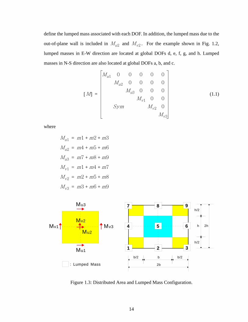
14

define the lumped mass associated with each DOF. In addition, the lumped mass due to the

out-of-plane wall is included in and . For the example shown in Fig. 1.2,

lumped masses in E-W direction are located at global DOFs d, e, f, g, and h. Lumped

masses in N-S direction are also located at global DOFs a, b, and c.

(1.1)

where

Figure 1.3: Distributed Area and Lumped Mass Configuration.

Mu2 Mv2

M[ ]

Mu1 0 0 0 0 0

Mu2 0 0 0 0

Mu3 0 0 0

Mv1 0 0

Sym Mv2 0

Mv3

=

Mu1 m1 m2 m3+ +=

Mu2 m4 m5 m6+ +=

Mu3 m7 m8 m9+ +=

Mv1 m1 m4 m7+ +=

Mv2 m2 m5 m8+ +=

Mv3 m3 m6 m9+ +=

1 2 3

4 5 6

7 8 9

2b

2h

h/2

h/2

h

b/2 b/2b

: Lumped Mass

Mu3

Mu1

Mu2Mv1

Mv2Mv3

15

1.4.5 Idealization of foundation conditions

As compared to the rigid base, the effect of flexible base can be an important factor

causing a decrease in the natural frequency of the structure (Hjelmstad et al., 1988). The

flexibility of the base can greatly affect the fundamental frequency if the stiffness of soil is

relatively small compared to the stiffness of the rigid support. A substantial part of the

vibration energy may be dissipated into the supporting medium by radiation of waves and

by hysteric action in the soil. In this work, soil-structure interaction is modeled where

necessary by using equivalent linear springs under each wall corresponding to the direc-

tion of ground motion.

1.4.6 Idealization of ground motions

The recorded motions utilized in the studies by Tena-Colunga and Abrams (1992a)

and the artificial ground motions proposed by Wen et al. (1999) are used in this research.

For the Gilroy firehouse studied by Tena-Colunga and Abrams (1992a), both single and

multiple recorded ground accelerations from the Loma Prieta earthquake are applied.

Because of the lack of significant ground motion records in the mid-America region, syn-

thetic ground motions generated by Wen are used to evaluate the performance of the half-

scale test building (Cohen 2000). For the non-linear time history analysis, the ground

motion of representative soil in Carbondale, Illinois site at the 2% in 50 years level is used

in these shaking table tests.

1.4.7 Damping Assumptions

Among many different damping assumptions, Rayleigh damping is the most popu-

lar for the structure-damping matrix because of its simplicity and computational advan-

tages. In this approach, the damping matrix is taken proportional to the stiffness and to the

mass matrices, i.e.,

16

(1.2)

where

= Rayleigh Damping Matrix

= Mass proportional damping influence coefficient

= Stiffness proportional damping influence coefficient

= Mass Matrix

= Stiffness Matrix

Rayleigh damping is assumed throughout this research. Issues associated with this

simplified damping model within the context of nonlinear dynamic analysis are discussed

in Section 4.3.6.

1.5 Overview of proposed linear static methodology for structures with flexible

diaphragms

Current seismic codes and standards generally use a single degree-of-freedom

(SDOF) model for low-rise buildings with rigid diaphragms, as shown in Fig. 1.4(a).

However, flexible diaphragm structures behave in general in the manner of a MDOF

model, as is shown in Fig. 1.4(b). A proposed simplified linear static methodology, appli-

cable to buildings with flexible diaphragms (i.e., applicable to buildings in which the dia-

phragm stiffness is small enough such that torsional coupling effects may be neglected) is

summarized in this section.

C a0M a1K+=

C

a0

a1

M

K

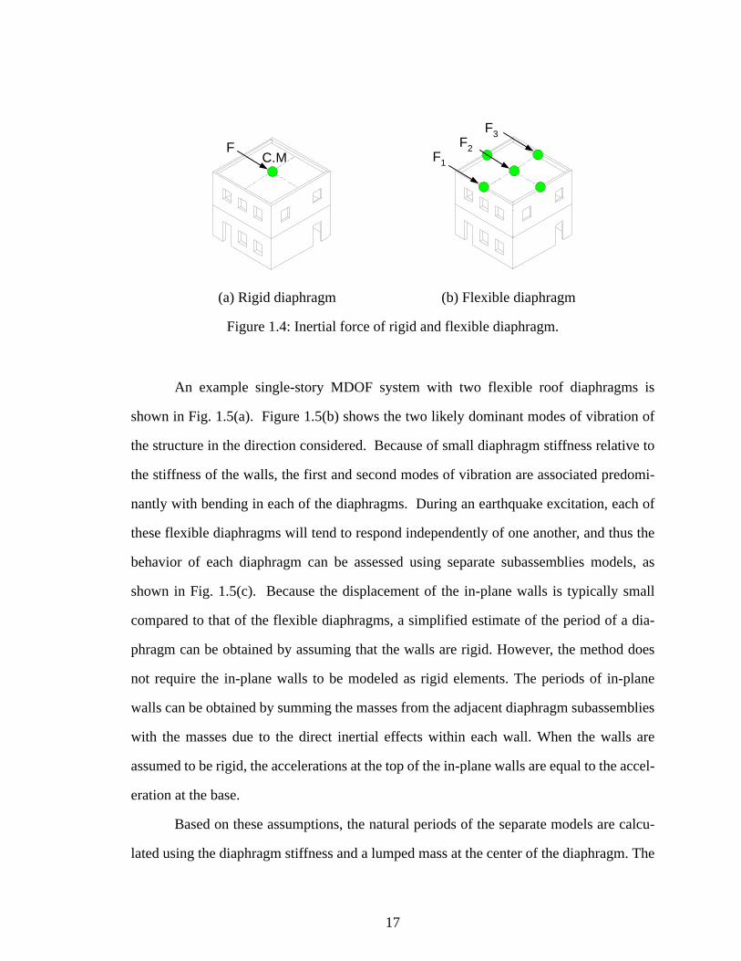
17

(a) Rigid diaphragm (b) Flexible diaphragm

Figure 1.4: Inertial force of rigid and flexible diaphragm.

An example single-story MDOF system with two flexible roof diaphragms is

shown in Fig. 1.5(a). Figure 1.5(b) shows the two likely dominant modes of vibration of

the structure in the direction considered. Because of small diaphragm stiffness relative to

the stiffness of the walls, the first and second modes of vibration are associated predomi-

nantly with bending in each of the diaphragms. During an earthquake excitation, each of

these flexible diaphragms will tend to respond independently of one another, and thus the

behavior of each diaphragm can be assessed using separate subassemblies models, as

shown in Fig. 1.5(c). Because the displacement of the in-plane walls is typically small

compared to that of the flexible diaphragms, a simplified estimate of the period of a dia-

phragm can be obtained by assuming that the walls are rigid. However, the method does

not require the in-plane walls to be modeled as rigid elements. The periods of in-plane

walls can be obtained by summing the masses from the adjacent diaphragm subassemblies

with the masses due to the direct inertial effects within each wall. When the walls are

assumed to be rigid, the accelerations at the top of the in-plane walls are equal to the accel-

eration at the base.

Based on these assumptions, the natural periods of the separate models are calcu-

lated using the diaphragm stiffness and a lumped mass at the center of the diaphragm. The

C.MF F2

F1

F3

18

lateral inertia forces at the center of the diaphragms are calculated from the period of the

separate models using the spectral acceleration. The lateral inertia forces of the in-plane

walls are calculated based on the peak ground acceleration and the lumped mass at the top

of the walls. The lateral forces at the center of the diaphragms are distributed to the adja-

cent in-plane walls. The reaction forces at the base of the walls are taken as the sum of the

lateral forces from the diaphragms plus the lateral forces of the in-plane walls. This

method is referred to in this research as the structural separation method.

Figure 1.5: Structural separation method for a story building with two flexible diaphragms.

A structure with two flexiblediaphragms

Diaphragm Lumped mass

Shear Wall

+Model 1 Model 2

Separated subassemblage models

1st Mode

2nd Mode

Two dominant modes

(a) (b)

(c)

19

1.6 Organization

The main body of the report is subdivided into four chapters. Chapter II summa-

rizes the implementation of the proposed MDOF analysis approach. Horizontal roof and

floor diaphragms, shear walls, and general hysteretic models for the wall and diaphragm

elements are considered. This chapter discusses wall and diaphragm element formula-

tions, and the strength, stiffness, and hysteretic response of the structural elements.

Chapter III applies the simplified MDOF model to a two-story historic building

with multiple diaphragms from Tena-Colunga and Abrams (1992). The main objective is

that the simplified multiple-degree-of-freedom (MDOF) models discussed in Chapter I

can be used for structural assessment of low-rise buildings with flexible floor diaphragms.

Time history analysis results are compared to measured field data.

Chapter IV provides a detailed analysis of the simplified MDOF model for a half-

scale one-story test building with a single nonrigid diaphragm from Cohen (2000a). A

calibration process is introduced and applied with the non-linear time history analyses of

the building to determine the model’s structural properties. After finishing the model cal-

ibration process, sensitivity analyses are performed to ascertain the influence of variations

in key parameters on the dynamic response.

Chapter V describes the simplified linear static procedure to assess low-rise build-

ings with flexible diaphragms. This chapter investigates structural separation procedure

using the two-story building discussed in Chapter III. The simplified procedure is applied

to linear elastic seismic assessment of the two-story and one-story buildings discussed in

Chapters III and IV, respectively. The resulting values are compared to those of linear

time history analysis for the buildings and implications relative to the inelastic seismic

response are addressed.

The research results are summarized and recommendations for seismic assessment

are provided in Chapter VI.

20

CHAPTER II

SIMPLIFIED ANALYSIS OF LOW-RISE BUILDINGS WITH NON-RIGID DIAPHRAGMS

2.1 Introduction

Prediction of the behavior of structures with rigid diaphragms is relatively easy

compared to that of the structures with flexible diaphragms. When the diaphragms do not

deform appreciably, horizontal forces are distributed to the lateral load resisting elements

in direct proportion to their relative rigidities. On the other hand, in building structures

with flexible diaphragms, the distribution of horizontal forces to the lateral load resisting

elements can depend significantly on the rigidity of the diaphragms.

One goal of this research is the development of simplified multiple-degree-of-free-

dom (MDOF) models that can be used for structural assessment of low-rise buildings with

flexible floor diaphragms. Subsequently, these models can be used to develop guidelines

for evaluating the response of these types of structures, or potentially as assessment tools

along with guidance documents. The simplified linear/nonlinear three-dimensional analy-

sis approach presented here captures the essential response characteristics of low-rise

shear wall buildings with flexible floor diaphragms discussed in Chapter I.

Particular emphasis is placed on how three-dimensional torsional response of the

structural system can be addressed, as well as how the effects of potential significant non-

linearities can be included within the analysis. The suggested approach is essentially as

efficient as possible for rapid evaluation of physical buildings or test designs, and for con-

ducting large numbers of analyses within simulation studies, while capturing the three-

21

dimensional response characteristics discussed in Chapter I.

One wall and one diaphragm element are developed for the suggested simplified

MDOF approach. These elements can be applied generally to various types of low-rise

shear wall buildings, but in this research, the modeling is focused mainly on masonry

buildings with nonrigid diaphragms. The nonlinear wall element is capable of capturing

in-plane diagonal tension, bed joint sliding, rocking and toe crushing limit states in URM

shear walls under lateral loadings. Three representative hysteresis models: a general pur-

pose linear kinematic hardening model, a rocking model, and a general purpose three

parameter model that includes stiffness degradation, strength deterioration, and pinching,

are implemented for use within the wall and/or diaphragm elements. The formulation of

the wall and diaphragm elements is presented in this chapter. Section 2.2 presents a litera-

ture review of previous analysis models for buildings with nonrigid diaphragms. Section

2.3 derives the diaphragm model and discusses the calculation of the diaphragm stiffness

and strength. Section 2.4 explains the formulation of the wall models, including the calcu-

lation of the wall stiffness and strength. The primary focus is on unreinforced masonry

walls, since the assessment of unreinforced masonry structures is of key importance in the

MAE Center research program.

2.2 Literature Review

Low-rise masonry shear wall buildings with nonrigid diaphragms have been con-

structed extensively in many active seismic areas. However, few research studies have

been conducted to gain a detailed understanding of the behavior of these types of build-

ings. The majority of prior studies have been limited to flexible diaphragms or masonry

shear wall structural components. Prior studies of masonry building structural systems

with flexible diaphragms have focused primarily on linear elastic analysis models. The

prior research is summarized in this section to provide the authors’ motivation for the pro-

22

posed three-dimensional simplified nonlinear analysis model.

2.2.1 Experimental basis for analysis modeling of buildings with nonrigid diaphragms

This section focuses on several areas of prior experimental tests that provide

important information for understanding the behavior of shear wall buildings with non-

rigid diaphragms. For purposes of discussion, these experimental tests are subdivided into

the following categories: flexible diaphragms, in-plane unreinforced masonry walls, and

masonry buildings with flexible diaphragms.

Experimental tests of flexible diaphragms

Current APA design procedures for horizontal plywood diaphragms are based in

large part on tests by Countryman (1952), Stillinger and Countryman (1955), and Tissell

(1966). Carney (1975) presented a bibliography that includes references on test results and

design procedures for straight-sheathed and diagonally-sheathed wood diaphragms and

plywood diaphragms.

Due to the addition of Seismic Design Zone 4 to the Uniform Building Code

(ICBO 1976), and the resulting greater design accelerations, Tissell (1979) conducted

eleven tests to check if the above design procedures would accurately predict the perfor-

mance of diaphragms designed for much higher loads. These tests included cases with a

high density of fasteners, openings, glued plywood diaphragms, and two-layer diaphragms

(plywood overlay). Tissell and Elliot (1983) summarized these test results and proposed

corresponding design procedures.

A major experimental program of 14 diaphragm tests subjected to simulated earth-

quake loading was conducted by ABK (1981). The tested diaphragms included a steel

deck with a concrete slab, two steel decks without a concrete slab, five plywood dia-

phragms, three wood diaphragms composed of straight sheathing, and three diagonally-

sheathed wood diaphragms. These dynamic component tests were designed to incorporate

23

the nonlinear dynamic interaction between the mass of the out-of-plane walls and the hor-

izontal diaphragm of typical URM buildings. The diaphragms, 20 ft. x 60 ft. in dimension,

were excited in the direction orthogonal to the out-of-plane walls. The unfilled steel deck

diaphragms, in general, responded elastically with the exception of seam and weld fail-

ures, whereas the other tests exhibited significant nonlinearity.

Tissell and Rose (1993) tested five full-scale roof diaphragms. The intent of these

tests was to develop empirical relationships for predicting diaphragm performance and

determining diaphragm design recommendations, with an emphasis on construction simi-

lar to that used in single- and double-wide manufactured homes. These diaphragms were

unblocked, and four of the tests had length/width ratios larger than 4:1.

Although the tests referenced above generally involve repeated loading, none of

the tests in any of the above references include cyclic loading reversals.

Falk and Itani (1987) tested two plywood-sheathed walls, two gypsum board

sheathed walls, three plywood floor diaphragms, and three gypsum board sheathed ceil-

ings. The purpose of the tests was to determine the basic natural frequencies, damping

ratios, and nonlinear load-deflection characteristics of plywood and gypsum diaphragms

with and without openings. It was found that the diaphragm natural frequency decreases

and the damping ratio increases as the displacement of the diaphragm is increased. Calcu-

lated values of the damping ratio ranged from 9 to 34 percent of critical damping. It was

also found that the reduction in the stiffness of wall diaphragms with openings is approxi-

mately proportional to the fraction of the wall area occupied by the openings.

Since the late 1940s, numerous composite diaphragm tests (steel deck with con-

crete topping) have been performed for several steel deck manufacturers (Easterling and

Porter 1994a). However, most of these tests were proprietary, and thus there are few pub-

lished results. Subsequently, Easterling and Porter (1994a) performed cyclic static tests of

32 full-size steel-deck-reinforced concrete floor diaphragms to determine their behavioral

and strength characteristics. A sample hysteresis response is shown in this reference, and

24

complete hysteresis data is catalogued in referenced research reports upon which this

paper is based. Six diaphragms within this series were subjected to both in-plane and ver-

tical load. The tests were conducted in a cantilever configuration. Based on the results of

these experiments, the authors developed expressions for the strength and stiffness of the

diaphragms. These expressions are specific to the configurations tested, and incorporate

the strength and stiffness of edge connectors specific to steel frames. However, these test

results and models can potentially be extended to cases having other boundary conditions.

Nakashima et al. (1982) tested several reinforced concrete beam-supported floor

slabs. These tests were scale models of a portion of the floor system in a typical medium-

to high-rise reinforced concrete building, and were subjected to monotonic loading as well

as symmetric cycles of increasing amplitude to failure. The purpose of these tests was to

evaluate the in-plane strength, stiffness and deformation characteristics of these types of

diaphragms, and to perform a comparison with the results of analysis models. Hysteresis

results for one of the tests are shown in the paper. The paper also correlates the experimen-

tal results with a detailed nonlinear finite element model composed of rigid triangular ele-

ments connected by springs.

Peralta et al. (2000) investigated experimentally the in-plane performance of

reduced scale existing and rehabilitated wood floor and roof diaphragms with elements

and connection details typical of pre-1950's construction. The tests provided fundamental

information for definition of the yield strength and displacement, effective stiffness, and

post-yield stiffness in bi-linear representations of the response. It was observed that the

recommendations in FEMA 273 and FEMA 356 did not predict the backbone curves of

the diaphragm tests accurately.

In general, the following characteristics are exhibited within at least some of the

diaphragm tests referenced above, for each of the major diaphragm types (plywood,

straight- and diagonally-sheathed wood, steel deck with concrete topping, and concrete

slab):

25

1. Strength deterioration, i.e., a loss in maximum load capacity with cycling at a

constant range of displacement.

2. Stiffness degradation, i. e., a loss in unloading stiffness with an increasing num-

ber of cycles and/or with cycling at larger displacement amplitudes.

3. Pinching, i.e., development of a plateau or near plateau in the load-displace-

ment response within a given half-cycle, followed by a subsequent increase in

the stiffness and load resistance at larger displacement levels within the half-

cycle.

Experimental tests of masonry walls

Experimental testing and analytical modeling of multistory URM walls with open-

ings have been conducted in prior research. However, the experimental studies in this field

have been less extensive than analytical studies (Anand 1996). A major experimental test

program involving unreinforced masonry (URM) walls subjected to earthquake loading

was conducted by ABK (1981). These tests showed that the resistance to collapse depends

more on the peak velocity input at the base and top of the walls than on the peak relative

deformations induced between the top and bottom of the walls. Pomonis (1992) performed

six shaking table tests on various types of unreinforced masonry walls. These tests investi-

gated the damage related to the effects of strong ground motion parameters. Abrams

(1992) tested a series of unreinforced brick walls. He discussed that masonry walls or

piers need not be considered brittle, but can possess a large inelastic deformation capacity

if they fail in a rocking mode. It was also noted that the behavior of walls under in-plane

cyclic loading was not influenced by previous damage due to rocking, that is, essentially

zero strength deterioration and stiffness degradation were observed. Leiva and Klingner

(1994) tested six full-scale two-story reinforced concrete masonry walls with openings

under in-plane seismic loading. They compared the effectiveness of two different models -

26

a pier and a multiple story type collapse model - for determining the collapse mechanism

of perforated walls. Thirty-two equally reinforced masonry walls, subjected to different

imposed lateral displacement - monotonic and cyclic, static and dynamic - were tested by

Tomazevic et al. (1996a). As vertical load increased, lateral resistance of the walls was

increased. It was also reported that the values of lateral resistance obtained by imposing

the same displacement pattern dynamically were higher than those obtained by static load-

ing, and that the ultimate displacement and resistance obtained by monotonic loading is

higher than that obtained by cyclic loading.

Erbay and Abrams (2002) tested three full-scale, clay-unit masonry walls sub-

jected to slowly applied reversals of lateral displacement. The results showed that unrein-

forced masonry walls can have substantial amount of inelastic deformation and energy

dissipation capacity. Behavior of the URM walls tested was dominated by sliding shear

behavior at the wall base. One of the walls was rehabilitated using the Center-Core Tech-

nique. This rehabilitation scheme improved the sliding shear capacity through dowel

action as much as 20%. The authors suggested that the lateral-force behavior of the walls

rehabilitated with this method can be assumed to be the same as that for reinforced

masonry walls.

It is difficult to specify detailed information on the properties of URM walls

because these properties differ from region to region (Scawthorn 1986; Paulson 1990;

Abrams 1992; Page 1998). These types of walls often have been assumed to be brittle

(Abrams 1992). In order to predict the lateral resistance and the nonlinear behavior of

URM walls or pier elements, the behavior is typically idealized as one of the following

types of failure: pier rocking, bed-joint sliding, toe crushing and diagonal tension. In a pier

rocking mode, a slender wall rocks on its base and behaves as a rigid body. Bed-joint slid-

ing is governed by a large fracture of the mortar joint at the bed joints when cracks propa-

gate from one interface to other along the mortar joint. Toe crushing occurs when the

vertical compressive stress of the URM wall is larger than the masonry compressive

27

strength and the bottom corner of the wall is crushed. Diagonal tension failure occurs

when diagonal cracks form in the wall, due to large tension stresses.

Experimental tests of masonry buildings

Due to the limited capabilities of laboratory facilities and testing equipment,

detailed information on full size building response is still very limited (Paulson and

Abrams 1990).

Tomazevic (1990) studied the influence of structural layout and reinforcement on

the seismic behavior of a three- to four- story residential masonry building. A small-scale

masonry building was tested by Tomazevic and Velechovsky (1992). Tomazevic and

Weiss (1994) tested two typical Central European three-story plain- and reinforced-

masonry buildings containing a reinforced concrete ribbed slab. The plain masonry tests

showed that cracks occurred between the walls and slabs.

In cooperative research between U.S. and Japan, a 5-story full-scale prototype

structure was tested in both countries. Yamazaki (1988a and 1988b) reported on the Japa-

nese 5-story full scale reinforced concrete masonry test. As the final validation of the

TCCMAR/US (U.S. Technical Coordinating Committee for Masonry Research) design

philosophy and analytical models, Seible (1994) reported on the U.S. full-scale five-story

building test. The U.S. test consisted of fully grouted masonry walls and precast pre-

stressed hollow-core plank floors with reinforced concrete topping, subjected to simulated

seismic loads.

Costley and Abrams (1996) investigated the dynamic behavior of two reduced-

scale single bay two-story URM buildings with flexible diaphragms. The test buildings

had steel floor systems which were designed to simulate the wood diaphragms. Approxi-

mately 40 channels of data from accelerometers and displacement transducers were col-

lected on each test structure. A total of 12-earthquake simulations, which were taken from

the Nahanni Earthquake, were performed with the first test structure. The last five studies

28

used a filtered displacement time history. Each earthquake simulation increased the inten-

sity of the base motion with respect to the previous simulation with the accelerations rang-

ing from 0.15g to 1.8g. Four earthquake simulations were performed with the second

structure. The intensity of the motion was increased from 0.2 g to 1.1 g in this test. The

test results and comparisons with various analytical models were reported.

Tomazevic and Klemenc (1997) performed two shaking table tests of a typical

confined masonry building. These tests were intended to confirm Eurocode 8. Modeling

the confined masonry shear walls as frames was considered as a rational analytical

method.

Paquette and Bruneau (2000) tested a single-story full-scale unreinforced brick

masonry building with wood diaphragms. They assessed the effectiveness of fiberglass

strips to improve the rocking behavior and compared the results with predictions from

existing seismic evaluation methodologies.

Cohen et al. (2000 a and b) tested two single-bay one-story half-scale reinforced

masonry buildings with flexible roof diaphragms. The first test had a diagonally sheathed

lumber diaphragm, and the second had a corrugated metal deck diaphragm. The structures

were subjected to artificial ground motions developed for the Mid-America region. The

test results showed that the structures did not behave as a single degree-of-freedom sys-

tem. The flexible roof diaphragms tended to behave independently of the two side in-plane

shear walls in these tests.

2.2.2 Prior and potential models for analysis of buildings with nonrigid diaphragms

In order to investigate the effect of the diaphragm flexibility on low-rise shear wall

buildings with nonrigid diaphragms, a wide range of analysis models have been developed

in prior research. Some of the most relevant models pertaining to the present work are

summarized below.

A detailed lumped parameter model was created in (ABK 1981) to characterize the

29

experimental diaphragm tests discussed in Section 2.2.1. This model has five degrees-of-

freedom distributed over one-half of the width of the diaphragm and connected by springs

and viscous dampers to represent the internal diaphragm response. The model is based on

assumed symmetry about the mid-span of the diaphragms, and includes lumped masses

from the diaphragm and the out-of-plane walls. Detailed plots of the experimental and

analytical diaphragm hysteresis behavior are provided in the report.

Cohen et al. (2000 a and b) developed a two degree-of-freedom idealized model of

their test buildings, also discussed in Section 2.2.1. The first DOF of the model is associ-

ated with the in-plane deformation of the narrow end shear walls (assumed equal due to

symmetry), and the second DOF is associated with the flexural deformation of the dia-

phragm (and the corresponding out-of-plane deformation of the longer walls). This model

can be represented as shown in Fig. 2.1(a). The calculated responses from this simplified

model are compared with the measured responses in the reports. This two-DOF model

cannot capture the significant contribution of the out-of-plane walls to the building lateral

stiffness and strength and torsional effects associated with incidental or intentional non-

symmetry of the stiffness and/or mass.

Practical modeling of URM buildings for design and/or assessment purposes has

been carried out by a number of investigators using two-dimensional discrete models.

Tena-Colunga and Abrams (1992a, 1992b, and 1996) examined the dynamic response of a

two-story URM building (a former firehouse in Gilroy, California) and a two-story rein-

forced masonry building located at Palo Alto during the Loma Prieta Earthquake. Data

was collected for the response of both buildings. Because the buildings were strong and

the earthquake motions were moderate, these structures remained predominantly within

the proportional limit. The accuracy and ease of use of a number of computational tech-

niques were evaluated, including the simple two-dimensional discrete linear-elastic

MDOF analytical model shown in Fig. 2.1(b) and a three-dimensional finite element

model such as illustrated in Fig. 2.1(d). Two-dimensional plane stress finite element mod-

30

els were used to estimate the stiffness of the in-plane masonry walls. In the discrete mod-

els, the in-plane masonry walls were modeled as condensed beam elements. The in-plane

stiffness coefficients of these beams were obtained from the two-dimensional plane stress

finite element analyses. The in-plane actions of the diaphragms were considered as elastic

shear springs in the direction of loading, considering in-plane shear resistance.

Figure 2.1: Analytical models: (a) Two DOFs model (Cohen 2000 a and b); (b) Lumped parameter model (Tena-Colunga and Abrams 1992a, 1992b, and 1996); (c) Equivalent frame model (Costley et al. 1996 and Kappos et al. 2002); and (d) Three-dimensional

Finite Element Model (Tena-Colunga et al. 1992 and Kappos 2002).

In the above studies, when the model shown in Fig. 2.1(b) is symmetric, it is iden-

tical with the one shown in Fig. 2.1(a).

31

An equivalent frame method (Tena-Colunga 1992, Kappos 2002), shown in Fig.

2.1(c), has been used by some investigators to model perforated shear walls. Kappos

(2002) performed two-dimensional nonlinear static pushover analyses using both Finite

Element and equivalent frame models to investigate the nonlinear behavior of perforated

walls. His equivalent frame model is composed of equivalent columns and beams with

rigid end zones. This method may not be accurate in some cases. The zones that are

assumed to be rigid often deform and crack (Tena-Colunga 1992).

Costley and Abrams (1996) investigated a number of conventional methods of

analysis to determine their applicability and accuracy in conjunction with their two

reduced-scale experimental tests (see Section 2.2.1). Beam and solid finite elements were

applied to determine the natural frequencies. To investigate the flexibility of the dia-

phragm, an isolated diaphragm model consisting of eleven floor beams was created to rep-

resent the experimental system. The experimental system involved steel bars that were

framed into the masonry with pinned ends, and each of these components were repre-

sented explicitly in the diaphragm model. The diaphragm model was used to check how

the diaphragm would behave within the overall structure. To represent the masonry por-

tion of the test buildings, eight-node solid elements were used. Two common analysis

methods, response spectrum and pushover analysis, were used. Also, a lumped parameter

three degree-of-freedom nonlinear dynamic model, similar in form to the one shown in

Fig. 2.1(b), was developed to estimate the post-cracking response of the structures. Cost-

ley and Abrams suggested that there was a need for improved simplified models for esti-

mating the response maxima of URM buildings.

Shing and Klingner (1998) used a state-of-the-art finite element program to inves-

tigate possible failure mechanisms of URM walls in a qualitative manner and to provide

guidance for the repair and retrofit of existing structures.

All of the above simplified MDOF models are two-dimensional lumped parameter

models. In all of these models, the nonrigid diaphragms and shear walls are idealized as

32

beams or shear springs. The only three-dimensional models involve the use of solid finite

elements, and these models are linear elastic. Isolated components have been modeled by

more complex two-dimensional nonlinear finite element capabilities. However, the exten-

sion of these sophisticated nonlinear models to general three-dimensional building

response is difficult both due to the lack of consideration of three-dimensional effects in

their development as well as the associated computational expense. Many of the prior

studies of overall structural systems have focused primarily on elastic, or linearized, build-

ing responses.

In order to improve the seismic assessment of shear wall structures with nonrigid

diaphragms, a new simplified three-dimensional nonlinear MDOF modeling approach is

proposed in this Chapter. The general characteristics of this model have been summa-

rized in Chapter I, Section 1.4.

2.3 Diaphragm Models

A building generally consists of horizontal floor and roof diaphragms and vertical

elements. The floor and roof diaphragms, which are typically assumed in design to behave

as horizontal deep beams or plate girders, distribute the lateral forces among the vertical

lateral-load resisting elements. The distribution of the horizontal forces to the vertical ele-

ments depends on the geometry and the rigidity of the diaphragms. Diaphragms can be

classified as nonrigid or rigid. Section 2.3.1 discusses how flexible diaphragms have been

idealized in prior research and practice. Section 2.3.2 presents the formulation of a new

diaphragm element. The element has six DOFs and is based on a force (equilibrium)

approach. An equivalent shear modulus is used in calculating the diaphragm stiffness.

Section 2.3.3 explains the idealization of multiple diaphragm structures in this work, i.e.,

the assumed connectivity between adjacent diaphragm elements. Section 2.3.4 discusses

the two basic types of diaphragm force-deformation models utilized in this work, i.e., non-

33

linear hysteretic models and equivalent linear models, and the basic properties associated

with each of these models. Section 2.3.5 discusses specific equivalent linear properties for

different diaphragm types, as well as the implications of various diaphragm approxima-

tions.

2.3.1 Proposed diaphragm idealization

As shown in Fig. 2.2, diaphragms are typically modeled using a plate girder anal-

ogy to idealize their behavior (ATC 1981). The boundary members of the diaphragm serve

as the girder flange and are termed the chords of the diaphragm. The deck or sheathing

functions as the web.

Figure 2.2: Plate girder under the horizontal loading.

In this approach, the diaphragm chord is typically assumed to provide the only

contribution to bending resistance, i.e., the bending contribution of the web is ignored.

The compression or tension force in the chord is calculated by dividing the moment in the

diaphragm by the distance between centerlines of the chord elements. The "flange" force

determined by this procedure is conservative.

The web carries the shear forces induced by the horizontal loadings. Based on

mechanics of materials and the assumption of a homogeneous isotropic elastic material,

the web shear stress exhibits a parabolic, but typically near uniform, distribution through

WebFlange

FlangeLoad

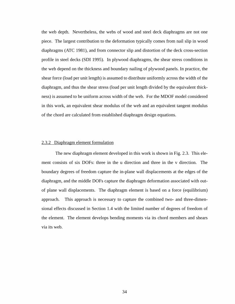
34

the web depth. Nevertheless, the webs of wood and steel deck diaphragms are not one

piece. The largest contribution to the deformation typically comes from nail slip in wood

diaphragms (ATC 1981), and from connector slip and distortion of the deck cross-section

profile in steel decks (SDI 1995). In plywood diaphragms, the shear stress conditions in

the web depend on the thickness and boundary nailing of plywood panels. In practice, the

shear force (load per unit length) is assumed to distribute uniformly across the width of the

diaphragm, and thus the shear stress (load per unit length divided by the equivalent thick-

ness) is assumed to be uniform across width of the web. For the MDOF model considered

in this work, an equivalent shear modulus of the web and an equivalent tangent modulus

of the chord are calculated from established diaphragm design equations.

2.3.2 Diaphragm element formulation

The new diaphragm element developed in this work is shown in Fig. 2.3. This ele-

ment consists of six DOFs: three in the u direction and three in the v direction. The

boundary degrees of freedom capture the in-plane wall displacements at the edges of the

diaphragm, and the middle DOFs capture the diaphragm deformation associated with out-

of plane wall displacements. The diaphragm element is based on a force (equilibrium)

approach. This approach is necessary to capture the combined two- and three-dimen-

sional effects discussed in Section 1.4 with the limited number of degrees of freedom of

the element. The element develops bending moments via its chord members and shears

via its web.

35

Figure 2.3: (a) MDOF model of one bay one-story building with four in-plane shear walls, (b) Six degree-of-freedom diaphragm element.

The element has four sampling points, one for each quadrant of the diaphragm as

shown in Fig. 2.4(a). Different uniform shear stresses exist in each quadrant due to the

lumped horizontal loadings at each of the DOFs. Specifically, the different shear stresses

in each quadrant are caused by the lumped loadings at DOFS u2 and v2 shown in Fig. 2.3.

(a) (b)

Figure 2.4: (a) Mesh of diaphragm element showing 4 sampling points in each quadrant (b) General deformation of diaphragm element.

Wall Element

Diaphragm Element

Wall ElementBoundary

: Node

: Direction of DOF

MDOF model Diaphragm Element

(a) (b)

u1

u3

u2 v3v1

v2

4

1

3

25

6

b b

h

h

τ1, γ1τ2, γ2

τ3, γ3τ4, γ4

u

v

1 2

4 3

36

Also, the shear stresses may differ in each quadrant because the properties of the

diaphragm may not be uniform due to openings, cutouts and changes in diaphragm thick-

ness or type. Openings through diaphragms for stairways, shafts, skylights, etc., can cause

a reduction in the stiffness and capacity of the diaphragms to resist lateral forces. In the

proposed approach, diaphragm openings are addressed by use of a reduced stiffness con-

tribution from the quadrants in which the openings are contained. Furthermore, in a non-

linear analysis, the shear stresses (and shear stiffnesses) within each quadrant may differ in

the post-elastic range of the response even if the initial properties are the same.

It is assumed that uniform shear strains are produced over the entire diaphragm

area by shear raking distortions associated with relative in-plane wall displacements in the

u and v directions. Figure 2.4 (b) illustrates the combination of this shear raking deforma-

tion with the bending deformations in the u and v directions. If the diaphragm properties

are the same within each of its quadrants, the shear raking distortions of course produce a

corresponding uniform shear stress throughout the diaphragm. However, if the diaphragm

properties are different in each quadrant, the idealized uniform shear raking distortions

produce different shear stresses in each quadrant.

To minimize the number of degrees-of-freedom, axial elongation and shortening of

the diaphragm is neglected in this research. These deformations may be included in gen-

eral by the use of independent axial springs between the out-of-plane walls and the middle

diaphragm DOFs.

Section 2.3.2.1 discusses the transformation between the global displacements of

the six-DOF diaphragm element and its three independent natural or deformational modes

of displacement (two bending modes and a shear raking mode). Section 2.3.2.2 presents

the formulation of the natural flexibility matrix, which is based on the above three natural

modes. Section 2.3.2.3 summarizes the calculation of the element stiffness matrix from

the flexibility matrix of Section 2.3.2.2 and the transformation matrix of Section 2.3.2.1.

Section 2.3.2.4 discusses the state determination procedure for nonlinear static and

37

dynamic analysis.

2.3.2.1 Transformation matrix

Consider the diaphragm element shown in Fig. 2.3(b). The nodal displacements of

this element can be subdivided into six independent modes {di} (see Fig. 2.5). The first

three modes, labeled as 1, 2 and 3 in Fig. 2.5, are referred to as deformational or natural

(Argyris et al. 1979) modes. The next three (labeled as 4, 5 and 6) are rigid body modes.

The three natural modes may be written as

Figure 2.5: Independent displacement modes of a diaphragm element (three natural modes and three rigid body modes).

(2.1)

6

1 2 3

54

y, v

x, u

- Three Natural Modes

- Three Rigid Body Modes

d1{ }

0

uN

0

0

0

0⎩ ⎭⎪ ⎪⎪ ⎪⎪ ⎪⎪ ⎪⎨ ⎬⎪ ⎪⎪ ⎪⎪ ⎪⎪ ⎪⎧ ⎫

= d2{ }

0

0

0

0

vN

0⎩ ⎭⎪ ⎪⎪ ⎪⎪ ⎪⎪ ⎪⎨ ⎬⎪ ⎪⎪ ⎪⎪ ⎪⎪ ⎪⎧ ⎫

= d3{ }

γ– Nh

0

γNh

γ– Nb

0

γNb⎩ ⎭⎪ ⎪⎪ ⎪⎪ ⎪⎪ ⎪⎨ ⎬⎪ ⎪⎪ ⎪⎪ ⎪⎪ ⎪⎧ ⎫

=

38

and the three rigid body modes may be expressed as

(2.2)

where

(2.3)

(2.4)

(2.5)

(2.6)

(2.7)

(2.8)

2b = diaphragm width in the u direction (see Fig. 2.3)

2h = diaphragm span length in the v direction (see Fig. 2.3)

The terms uN and vN in Eqs. 2.1, 2.3 and 2.5 are element natural displacements, or

element deformations, associated with diaphragm bending. These deformations are

obtained as the difference between the total displacement at the middle of the diaphragm

d4{ }

uR

uR

uR

0

0

0⎩ ⎭⎪ ⎪⎪ ⎪⎪ ⎪⎪ ⎪⎨ ⎬⎪ ⎪⎪ ⎪⎪ ⎪⎪ ⎪⎧ ⎫

= d5{ }

0

0

0

vR

vR

vR⎩ ⎭⎪ ⎪⎪ ⎪⎪ ⎪⎪ ⎪⎨ ⎬⎪ ⎪⎪ ⎪⎪ ⎪⎪ ⎪⎧ ⎫

= d6{ }

θRh

0

θ– Rh

θ– Rb

0

θRb⎩ ⎭⎪ ⎪⎪ ⎪⎪ ⎪⎪ ⎪⎨ ⎬⎪ ⎪⎪ ⎪⎪ ⎪⎪ ⎪⎧ ⎫

=

uN u2

u1 u3+2

-------------------–=

uR

u1 u3+2

-------------------=

vN v2

v1 v3+2

-------------------–=

vR

v1 v3+2

-------------------=

γN12---

v3 v1–2b

------------------u3 u1–

2h------------------+⎝ ⎠

⎛ ⎞=

θR12---

v3 v1–2b

------------------u3 u1–

2h------------------–⎝ ⎠

⎛ ⎞=

39

and the average of the corresponding displacements at the diaphragm edges (see Fig. 2.6).

The third natural displacement, , is associated with the shear raking in mode 3 of the

diaphragm as shown in Fig. 2.5. The total shear strain induced by this mode is equal to

, where is defined by Eq. 2.7.

Figure 2.6: Calculation of the diaphragm deflection.

Given the above relationships, the natural displacements may be related to the total

displacements by the following matrix form:

or (2.9)

(2.10)

where

γN

2γN γN

Diaphragm

WallWall

Lateral load

Diaphragm

u1

u1 u3

u3

uN

u2

uN

u1+u3

2

dN{ } T[ ] d{ }=

uN

vN

γN⎩ ⎭⎪ ⎪⎪ ⎪⎨ ⎬⎪ ⎪⎪ ⎪⎧ ⎫

T[ ]

u1

u2

u3

v1

v2

v3⎩ ⎭⎪ ⎪⎪ ⎪⎪ ⎪⎪ ⎪⎨ ⎬⎪ ⎪⎪ ⎪⎪ ⎪⎪ ⎪⎧ ⎫

=

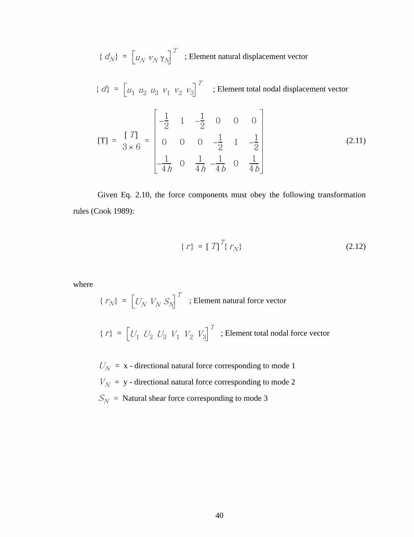
40

; Element natural displacement vector

; Element total nodal displacement vector

[T] = (2.11)

Given Eq. 2.10, the force components must obey the following transformation

rules (Cook 1989):

(2.12)

where

; Element natural force vector

; Element total nodal force vector

= x - directional natural force corresponding to mode 1

= y - directional natural force corresponding to mode 2

= Natural shear force corresponding to mode 3

dN{ } uN vN γN

T=

d{ } u1 u2 u3 v1 v2 v3

T=

T[ ]3 6×

12---– 1

12---– 0 0 0

0 0 012---– 1

12---–

14h-------– 0

14h------- 1

4b-------– 0

14b-------

=

r{ } T[ ]T rN{ }=

rN{ } UN VN SN

T=

r{ } U1 U2 U3 V1 V2 V3

T=

UN

VN

SN

41

2.3.2.2 Natural Flexibility Matrix

The natural flexibility matrix is formulated based on the 3 natural modes in Fig.

2.5. The coefficients of the natural flexibility matrix

(2.13)

are obtained by subjecting the element to a unit load at each of the natural DOFs, with the

displacements in the three rigid-body modes held to zero. The flexibility coefficient

is the ith displacement due to a unit load at the jth natural DOF. The following sub-

section derives the diagonal flexibility coefficients corresponding to the element bending

modes (the first and second columns of Eq. 2.13). This is followed by the derivation of

the diagonal flexibility coefficients corresponding to the element shear raking mode (col-

umn three of Eq. 2.13).

Flexibility coefficients corresponding to the diaphragm bending modes.

Consider the diaphragm deformations in mode 1 of Fig. 2.5 induced by a unit force

applied at the center of the diaphragm, as shown in Fig. 2.7. This force produces uniform

shear stresses in each of the diaphragm’s quadrants as shown on the right side of Fig. 2.7.

The resulting total displacement at the center of the diaphragm can be expressed as the

sum of the bending displacement due to shear deformation of the diaphragm web plus the

displacement due to flexural deformation of the diaphragm chords. That is,

FN[ ]

3 3×

FN11FN12

FN13

FN21FN22

FN23

FN31FN32

FN33

=

FNij

42

Figure 2.7: Internal stress distributions due to horizontal unit force, UN = 1.

(2.14)

where

= bending deflection due to web shear deformation

= bending deflection due to chord deformation

For a diaphragm with uniform properties throughout its area

( ), the diaphragm center-span displacement can be calcu-

lated (from virtual work) as

(2.15)

where

= shear modulus of the web for quadrant i = 1, 2, 3, 4.

In the context of linear analysis, these coefficients are the elastic (or equivalent elastic)

+

- -

+G1 G2

G3G414bt

14bt

14bt

14bt

14bt

14bt

14bt

14bt

14bt

14bt

14bt

14bt

G1 G2

G3G4

1/2

1/2

1 h

h

b b

FN11∆S ∆C+=

∆S

∆C

G G1 G2 G3 G4= = = =

∆S1

4bt( )2----------------- 1

G1

------- 1G2

------- 1G3

------- 1G4

-------+ + + t x ydd0

h

∫0

b

∫h

4btG--------------= =

Gi

43

shear moduli within each of the diaphragm quadrants. In the context of a nonlinear analy-

sis, these coefficients are the tangent shear moduli corresponding to the current state

within each of the diaphragm quadrants.

As noted previously, the shear modulus of each diaphragm quadrant may be differ-

ent due to openings in the diaphragm, irregular diaphragm properties, or diaphragm non-

linearity. In this general case, the diaphragm bending deflection due to web shear is

calculated as

(2.16)

The displacement due to diaphragm chord deformation may be expressed in gen-

eral as the sum of the effects due to the flexural strains generated in the chords plus that

due to slippage within the chord splices (ATC 1981), i.e.,

(2.17)

where

= bending deflection due to flexural strains in the chord members

= bending deflection due to the chord splice slip in the chord members

The bending deflection due to flexural strains within the chord members is

(2.18)

∆S1

4bt( )2----------------- 1

G1

------- 1G2

------- 1G3

------- 1G4

-------+ + + t x ydd0

h

∫0

b

∫=

h16bt( )

------------------ 1G1

------- 1G2

------- 1G3

------- 1G4

-------+ + +=

∆C ∆cb ∆cs+=

∆cb

∆cs

∆cb2h( )3

48EI--------------- h

3

6EI----------= =

44

where

= elastic modulus of the chord members

= moment of inertia contribution from the chord members

2h = diaphragm span length in v direction

Based on virtual work principles, the bending deflection due to slip at a single

chord splice location may be written as

(2.19)

where

= slip at the chord splice location

= location of chord splice relative to the end of the diaphragm

The total deflection due to slip at all the chord splices is obtained by summing the

contributions from each of the chord splice locations. Therefore, for the example shown

in Fig. 2.8, the bending deflection due to slip is

(2.20)

The reader should note that Eqs. 2.19 and 2.20 are used to obtain an equivalent elastic

(secant) stiffness associated with an anticipated or specified slip at the chord splices. Non-

linear chord deformations are not considered in the present research. If chord inelastic

response is considered, tangent relationships for the chord flexural deformations and for

chord splice slip are needed.

E

I 2Ab2=

∆cs ∆slip

Xs

4b-------⎝ ⎠

⎛ ⎞=

∆slip

Xs

∆cs ∆elongation ∆shortening+( )Xs

4b-------⎝ ⎠

⎛ ⎞=

45

Figure 2.8: Example bending deflection due to chord splice slip.

For a diaphragm with uniform shear properties (i.e., and

constant effective thickness), the off diagonal flexibility coefficients in Eq. 2.13 are zero.

However, in the general case in which these properties differ between any of the quadrants

of the diaphragm, displacements are produced at all of the natural degrees of freedom due

to a force at any one of these degrees of freedom. Based on virtual work and considering

Figs. 2.7 and 2.9, the off-diagonal flexibility coefficient is derived as follows:

∆cs

G1 G2 G3 G4= = =

FN12

46

Figure 2.9: Internal stress distributions due to vertical unit force, VN = 1.

(2.21)

The flexibility coefficient is equal to by symmetry.

Flexibility coefficients corresponding to the shear raking mode.

For the third natural mode in Fig. 2.5, the nodal forces due to a given natural shear

force may be calculated as:

1

1/21/2 14ht

14ht

14ht

14ht

14ht

14ht

14ht

14ht

14ht

14ht

14ht

14ht

+

+ -

-G1 G2

G3G4

G1 G2

G3G4 h

h

b b

FN12

14bt( ) 4ht( )

----------------------------- 1G1

------- 1G2

-------– 1G3

------- 1G4

-------–+ t x ydd0

h

∫0

b

∫=

h16t( )

-------------- 1G1

------- 1G2

-------– 1G3

------- 1G4

-------–+=

FN21 FN12

SN

47

(2.22)

The nodal forces at the middle of the diaphragm, and , are zero in Eq. 2.22. The

other nodal forces are illustrated in Fig. 2.10. The associated internal shear stresses are

shown in Fig. 2.11.

Figure 2.10: Element shear raking mode and corresponding nodal forces.

U1

U2

U3

V1

V2

V3⎩ ⎭⎪ ⎪⎪ ⎪⎪ ⎪⎪ ⎪⎨ ⎬⎪ ⎪⎪ ⎪⎪ ⎪⎪ ⎪⎧ ⎫

T[ ]T0

0

SN⎩ ⎭⎪ ⎪⎨ ⎬⎪ ⎪⎧ ⎫

SN

4h-------–

0

SN

4h-------

SN

4b-------–

0

SN

4b-------

⎩ ⎭⎪ ⎪⎪ ⎪⎪ ⎪⎪ ⎪⎪ ⎪⎪ ⎪⎪ ⎪⎨ ⎬⎪ ⎪⎪ ⎪⎪ ⎪⎪ ⎪⎪ ⎪⎪ ⎪⎪ ⎪⎧ ⎫

= =

U2 V2

γN

γN

U3

V3

U1

b b

h

h

V1

48

Figure 2.11: Internal shear stress distribution in four quadrants of the diaphragm element for SN=1.

The diagonal flexibility coefficient associated with the shear raking natural mode,

, is obtained for the general case of an irregular diaphragm (i.e.,

), as

(2.23)

The off-diagonal flexibility coefficient is obtained for the general case in

which the diaphragm has nonuniform properties in a similar fashion to the derivation of

of the previous section. Based on virtual work, and considering Figs. 2.7 and

2.11, one obtains:

G1 G2

G3G4

+

+ +

+

18hbt

18hbt

18hbt

18hbt

18hbt

18hbt

18hbt

18hbt

18hbt

18hbt

18hbt

18hbt

h

h

b b

SN=114b

14b

14h

14h

G1 G2

G3G4

FN33

G1 G2 G3 G4≠ ≠ ≠

FN33

1

8bht( )2--------------------- 1

G1

------- 1G2

------- 1G3

------- 1G4

-------+ + + t x ydd0

h

∫0

b

∫=

164bht----------------- 1

G1

------- 1G2

------- 1G3

------- 1Ge4

----------+ + +=

FN31

FN12

49

(2.24)

The off-diagonal flexibility coefficient is derived in exactly the same man-

ner based on virtual work, and considering Figs. 2.9 and 2.11.

(2.25)

Finally, coefficients and are obtained by symmetry.

Flexibility Matrix

Based on the above developments, the 3 x 3 diaphragm natural flexibility matrix

can be summarized as

(2.26)

where

FN31

18bht( ) 4bt( )

--------------------------------- 1G1

------- 1G2

------- 1G3

-------– 1G4

-------–+ t x ydd0

h

∫0

b

∫=

132bt------------- 1

G1

------- 1G2

------- 1G3

-------– 1G4

-------–+=

FN32

FN32

18bht( ) 4ht( )

--------------------------------- 1G1

------- 1G2

-------– 1G3

-------– 1G4

-------+ t x ydd0

h

∫0

b

∫=

132ht------------- 1

G1

------- 1G2

-------– 1G3

-------– 1G4

-------+=

FN13 FN23

FN[ ]

3 3×

h16bt-------------D1

h3

6EIu------------- ∆csu+ + h

16t---------D2

132bt-------------D4

b16ht-------------D1

b3

6EIv------------- ∆csv+ + 1

32ht-------------D3

Sym1

64bht-----------------D1

=

50

(2.27)

(2.28)

(2.29)

(2.30)

= x-directional displacement due to the chord splice slip

= y-directional displacement due to the chord splice slip

= elastic modulus of the chord members

Iu = x- directional moment of inertia from the chord members

Iv = y- directional moment of inertia from the chord members

t = effective thickness of diaphragm web.

2.3.2.3 Element stiffness matrix

The 3 x 3 natural stiffness matrix is determined from the flexibility matrix

as

(2.31)

Given the natural stiffness, the 6 x 6 element global stiffness is obtained by fundamental

principles (Cook 1989) as

(2.32)

D11G1

------- 1G2

------- 1G3

------- 1G4

-------+ + +=

D21G1

------- 1G2

-------– 1G3

------- 1G4

-------–+=

D31G1

------- 1G2

-------– 1G3

-------– 1G4

-------+=

D41G1

------- 1G2

------- 1G3

-------– 1G4

-------–+=

∆csu

∆csv

E

KN[ ]

FN[ ]

KN FN

1–=

K TT

KN T=

51

2.3.2.4 State determination process

For nonlinear static or dynamic analysis, the diaphragm internal forces and the

stiffness matrix are evaluated and updated by tracking the state within each quad-

rant of the diaphragm. This process, which is referred to as element state determination, is

summarized in this section.

Given the incremental diaphragm displacements

(2.33)

which are obtained from the solution of the global tangent stiffness equations, the incre-

mental natural displacement vector is obtained as

(2.34)

The element incremental natural forces are then calculated via

(2.35)

where

; incremental natural forces

Based on these incremental natural forces, the incremental shear strains are calcu-

lated in each of the diaphragm quadrants as:

KN[ ]

∆d{ } ∆u1 ∆u2 ∆u3 ∆v1 ∆v2 ∆v3

T=

∆dN{ } T[ ] ∆d{ }=

∆rN{ } KN∆dN{ }=

∆rN{ } ∆UN ∆VN ∆SN

T=

52

(2.36)

(2.37)

(2.38)

(2.39)

These equations can be represented in matrix form as

(2.40)

Using Eq. 2.40, with , the quadrant incremental shear

stresses are

(2.41)

and if the response in a given quadrant is linear during this increment, the total shear

stresses may be updated using the equation

∆γ1

∆UN

4btG1

-----------------∆VN

4htG1

-----------------∆SN

8bhtG1

---------------------+ +=

∆γ2

∆UN

4btG2

-----------------∆VN

4htG2

-----------------–∆SN

8bhtG2

---------------------+=

∆γ3

∆UN

4btG3

-----------------–∆VN

4htG3

-----------------–∆SN

8bhtG3

---------------------+=

∆γ4

∆UN

4btG4

-----------------–∆VN

4htG4

-----------------∆SN

8bhtG4

---------------------+ +=

∆γ{ }

14btG1

----------------- 14htG1

----------------- 18bhtG1

---------------------

14btG2

----------------- 14htG2

----------------- 18bhtG2

---------------------

14btG3

----------------- 14htG3

----------------- 18bhtG3

---------------------

14btG4

----------------- 14htG4

----------------- 18bhtG4

---------------------

∆rN{ }=

G{ } G1 G2 G3 G4

T=

∆τ{ }

G1∆γ1

G2∆γ2

G3∆γ3

G4∆γ4

=

53

(2.42)

where

= shear stress in the quadrant at the beginning of the increment

If nonlinearities occur within the increment, the following sub-incrementation process is

employed to obtain the state at the end of the increment.

Sub-incrementation

Consider Figs. 2.12 and 2.13. Figure 2.12 shows the notation and sign convention

employed for the stresses and strains in each quadrant of the diaphragm. Within this work,

diaphragm nonlinear shear response is represented in a multi-linear fashion. Any number

of the quadrants of a diaphragm may experience some nonlinearity during a given incre-

ment. Figure 2.13 shows a hypothetical increment in which the stress-strain response is

nonlinear within the 1st, 2nd and 3rd quadrants. The subincrementation process starts by

calculating the fraction of the increment required to reach the first point of nonlinearity (or

change in stiffness) within all of the quadrants. This fraction is

(2.43)

in each quadrant

where

= a ratio of shear stress to trial shear stress for ith quadrant

= 1, 2, 3, 4 for four quadrants

= trial shear stress increment for ith quadrant

= for ith quadrant

τcur{ } τprev{ } ∆τ{ }+=

τprev{ }

αi

∆τyi

∆τi

-----------=

αi

i

∆τi

∆τyi τyi τprev_i–

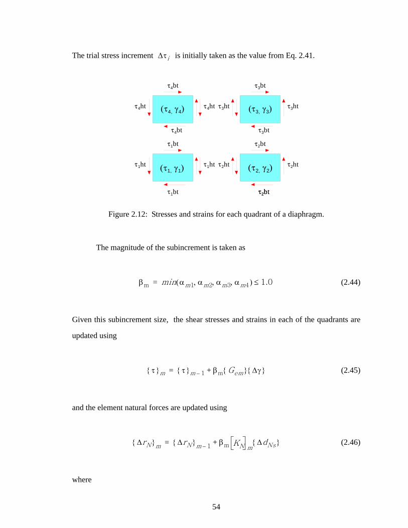
54

The trial stress increment is initially taken as the value from Eq. 2.41.

Figure 2.12: Stresses and strains for each quadrant of a diaphragm.

The magnitude of the subincrement is taken as

(2.44)

Given this subincrement size, the shear stresses and strains in each of the quadrants are

updated using

(2.45)

and the element natural forces are updated using

(2.46)

where

∆τi

(τ4, γ4)

τ4bt

τ1bt

τ1bt

τ1ht τ1ht

τ2bt

τ2btτ2bt

τ2ht τ2ht

τ3bt

τ3bt

τ3ht τ3ht

τ4bt

τ4htτ4ht

(τ1, γ1)

(τ3, γ3)

(τ2, γ2)

βm min αm1 αm2 αm3 αm4, , ,( ) 1.0≤=

τ{ }m τ{ }m 1– βm Gem{ } ∆γ{ }+=

∆rN{ }m

∆rN{ }m 1– βm KN m

∆dNs{ }+=

55

m = sub-incremental step (1, 2, 3, ..., m).

= accumulated shear stress at the end of the mth sub-increment

= accumulated shear stress at the beginning of the mth sub-incre-

ment

= natural tangent stiffness at the beginning of the mth sub-incre-

ment

The above process is repeated until the complete of Eq. 2.40 is applied. The

quadrant shear stiffnesses and the element natural stiffness are updated

throughout the subincrementation process based on the nonlinearity that is encountered

within each of the quadrants. At the end of this process, the current total nodal forces are

calculated from the element natural force vector using Eq. 2.12. This nodal force vector is

then exported to the global nonlinear incremental iterative solution algorithm.

Figure 2.13: Stress-strain diagram example for each quadrant of a diaphragm.

τ{ }m

τ{ }m 1–

KN m

∆γ{ }

Gi KN

VN

UN

SN

τ3

γ3

τ2

γ2

τ4

γ4

τprev_1

γ1

G1

τprev_2

τprev_3

τprev_4

τcur_1 τcur_2

τcur_3τcur_4

τ1

∆τy1∆τ1

∆γ1

G2

G3G4

Gt1Gt2

Gt3

∆τy2∆τ2

∆γ2

∆τ3∆τy3∆τ3

∆γ2

γprev_1 γprev_2

γprev_3γprev_4

γcur_1 γcur_2

γcur_3γcur_4

τy3

τy2τy1

c) 1st quad. d) 2nd quad.

b) 3rd quad.a) 4th quad.

G1G2

G3G4

56

2.3.3 Idealization of multiple diaphragms

The proposed diaphragm element, which has six DOFs, is discussed in Sections

2.3.1 and 2.3.2. When this element is used to model multiple adjacent diaphragms, the

associated idealizations may be explained as follows. Figure 2.14 (a) shows two adjacent

diaphragm elements, representing two adjacent floor or roof diaphragms with one interior

wall between them and exterior walls on their outside edges. DOF numbers 1 through 6

are assigned to the diaphragm on the left, and DOF numbers 7 through 12 are assigned to

the diaphragm on the right. DOFS 1, 2, 3, 7, 8, and 9 are in the x (or u) direction and

nodes 4, 5, 6, 10, 11, and 12 are in the y (or v) direction.

When the structure containing these diaphragms is loaded in the y direction, it is

assumed that the diaphragms will deform as shown in Fig. 2.14(b). That is, each of the

above diaphragms deforms effectively as a simply-supported beam between the interior

wall and the associated exterior wall. Continuity of the flexural deformations between the

two diaphragms is neglected. This assumption is considered to be appropriate for typical

masonry buildings with nonrigid diaphragms, since the in-plane wall displacements tend

to be small compared to the diaphragm displacements, and the diaphragm displacements

tend to be dominated by shear deformations. Also, these types of buildings would not

necessarily have any physical continuity of a diaphragm chord member across the interior

wall. Due to the significant flexural shear deformations within each of the diaphragm ele-

ments, any displacement discontinuities at the interior wall are expected to be small.

If deformations within the anchorages between the diaphragms and the interior

wall are small, neglected, or included implicitly within the description of the overall dia-

phragm force-deformation relationships, DOFS 6 and 10 may be shared as the same global

DOF. If the stiffness of the interior wall is reduced, e.g., due to damage or nonlinearity,

the displaced shape of the two diaphragm elements may become more like that shown in

Fig. 2.14(c). The resistance from the diaphragms to the y direction displacement of the

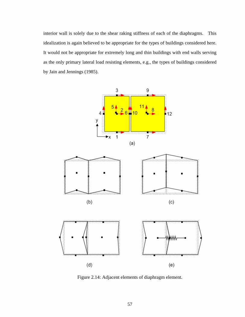
57

interior wall is solely due to the shear raking stiffness of each of the diaphragms. This

idealization is again believed to be appropriate for the types of buildings considered here.

It would not be appropriate for extremely long and thin buildings with end walls serving

as the only primary lateral load resisting elements, e.g., the types of buildings considered

by Jain and Jennings (1985).

Figure 2.14: Adjacent elements of diaphragm element.

58

When the above structure is loaded in the x direction, the deflected shapes of the

diaphragms might appear as shown in Fig. 2.14(d) unless the continuity of the mid-dia-

phragm u displacements is addressed. That is, a gap or overlap could occur between the

diaphragms. The continuity of the x direction displacements of the two diaphragms, and

the fact that some axial shortening or extension of the diaphragms may occur between the

walls, can be addressed by specifying an axial spring between the x-direction DOFS at the

middle of the diaphragms, as shown in Fig. 2.14 (e). This type of idealization was

employed by Tena-Colunga and Abrams (1992) within a two-dimensional analysis

approach. Alternately, a simpler MDOF model is obtained by assuming that the dia-

phragm middle DOFS are rigidly constrained to have the same displacement in the x

direction. This idealization is employed in this work for structures containing multiple

diaphragms. As previously explained in Section 1.4.3, the x direction wall degrees of

freedom, 1 and 7, and 3 and 9, are constrained to have equal displacements in this work.

2.3.4 Diaphragm force-deformation relationships

In the previous sections, a diaphragm idealization has been introduced and an asso-

ciated diaphragm element has been derived. The basic idealization is that the diaphragm

behaves as a deep plate girder with respect to bending deformations and as a uniformly

strained shear panel with respect to coupling of the walls at the diaphragm boundaries. As

noted in the above discussions, there are essentially two types of diaphragm force-defor-

mation models that are used in the context of this idealization: (1) a general nonlinear

hysteretic model and (2) an equivalent linear model. The key concepts and properties

associated with each of these models are discussed below.

59

2.3.4.1 Nonlinear force-deformation model

A typical nonlinear hysteretic response of a wood diaphragm, taken from (ABK

1981), is shown in Fig. 2.15(a). The diaphragm is subjected to static cyclic loadings as

illustrated in Fig. 2.15(b). The main phases of the cyclic behavior are loading, unloading

with stiffness degradation, pinching, and reloading with strength deterioration. The initial

loading path typically follows the virgin envelope determined by a monotonic loading test.

Figure 2.15: (a) Typical cyclic force-deformation model (ABK 1981); (b) Diaphragm subjected to distributed loading; and (c) Diaphragm subjected to lumped loading.

In this research, a three-parameter model similar to those developed by Kunnath et

al. (1991, 1994) is implemented to characterize the general diaphragm hysteresis behavior.

This model is also used to represent certain types of wall hysteresis. In this model, stiff-

ness degradation, strength deterioration and pinching are each described by a single

parameter or property. Stiffness degradation is characterized by a parameter symbolized

V

∆

(a) (b)

teff

V V

L

B

(c)

teff

V V

L

B

P

60

by the term , strength deterioration is represented by a parameter symbolized by the

term , and pinching addressed by a parameter symbolized by the term . The influence

of each of these parameters on the behavior of the nonlinear hysteresis model is explained

in detail in Appendix A.

Figure 2.16 gives a simple illustration of the concepts associated with the above

nonlinear hysteretic model. Figure 2.16(a) shows a trilinear representation used by the

model to represent the force-deformation response from a monotonic test. It is assumed

that this curve also represents the nonlinear backbone curve for the cyclic response with

sufficient accuracy (see Section 2.8.3 of FEMA 356 (ASCE 2000a) for discussion of the

backbone curve). Five properties of the nonlinear model are determined based on the

results of a monotonic test and are illustrated in Fig. 2.16(a): Vo, V1, K0, K1 and K2. One

can observe that K0 is the initial tangent stiffness of the virgin diaphragm, and Vo is the

proportional limit associated with the monotonic response. The term V1 might be referred

to as the ultimate strength of the diaphragm, although diaphragm forces greater than this

value are produced within the model. The terms K1 and K2 are post-elastic tangent stiff-

nesses associated with the trilinear representation of monotonic load-deformation

response.

Figure 2.16(b) shows an example cyclic prediction by the three-parameter hystere-

sis model, and illustrates the significance of the three hysteresis parameters , and .

As the reader might expect, it can be difficult to characterize the complex nonlinear hys-

teretic response of general diaphragms and other structural components by the use of only

three parameters. Example experimental results from a recent cyclic diaphragm test (Per-

alta et al. 2000) are shown in Fig. 2.17. The prediction of the response for diaphragm

MAE-2B is shown in Fig. 2.18. The pinching parameter is equal to infinity for this

case, indicating zero pinching. An example determination of the above three parameters

based on a cyclic diaphragm test, including pinching effects, is explained in Section 4.3.2.

α

β γ

α β γ

γ

61

Figure 2.16: Typical cyclic load deflection model using three parameter model: (a) A trilinear representation and (b) Three parameter model (See Appendix A).

(a)

(b)

V1

V0

K0

K1

K2

∆∆0 ∆1

V

∆

(Stiffness Degradation)

Virgin Envelope(Monotonic Loading)

( PinchingEffect )

αVy

γVy

dE

β∗dE/Vy

V1

V0

62

Figure 2.17: Specimen MAE-2. Load vs. displacement at loading points (Peralta et al. 2000).

-35

-30

-25

-20

-15

-10

-5

0

5

10

15

20

25

30

35

-3 -2.5 -2 -1.5 -1 -0.5 0 0.5 1 1.5 2 2.5 3

Displacement (inches)

Load

(kip

s)

MAE-2

MAE-2A

MAE-2B

MAE-2C

Note:1. MAE-2 - 24'x12' Roof diaphragm: 2"x10" joists with 1"x6" straight sheathing

2. MAE-2A - Steel truss underneath the diaphragm

3. MAE-2B - 3/8" Plywood overlay nailed on decking

4. MAE-2C - Blocking added and heavier nailing pattern

MAE-2

MAE-2A

MAE-2C

MAE-2BPhotographs DuringRetrofit and Test

63

Figure 2.18: Experimental test and predicted force and displacement force and displacement relationship using three parameter model( , , and ).

Diaphragm force-deformation models are typically expressed in terms of the max-

imum diaphragm shear force and a corresponding maximum diaphragm bending displace-

ment. That is, the nonlinear response associated with the shearing deformations within the

diaphragm web and the flexural deformations with the diaphragm chords (including nail

slip, chord splice slip, etc.) are all lumped into a single force-deformation relationship.

This is somewhat problematic if one wishes to determine a “rigorous” diaphragm force-

deformation relationship for combined bending in two orthogonal directions along with

diaphragm shear raking displacements.

For many of the diaphragm types used in masonry building structures, the dia-

phragm is dominated by the shear response of its web. This assumption is implicit within

the development of the diaphragm element proposed in this work. It is assumed in this

work that the chord flexibility can be represented sufficiently by an elastic or equivalent

elastic model. In many situations, the chord stiffness is even large enough relative to the

stiffness of the diaphragm in shear such that the chord can effectively be modeled as rigid.

Based on these assumptions, the diaphragm shear force (per unit length) versus shear

-20

-15

-10

-5

0

5

10

15

20

-1 -0.5 0 0.5 1

Displacement (inches)

Load

(kip

s)

MAE-2B(Exprimental test)

MAE-2B (Threeparameter model)

α 6.0= β 6.0= γ ∞=

64

strain relationship, which is required within the proposed element, can be derived from

test results by representing the test by the associated lumped parameter idealization as

shown in Fig. 2.15(c). The idealization of the chord response is established first, and the

shear-force shear-strain relationship is then obtained by equating the predicted displace-

ments in the analysis model, based on the lumped loading at the middle of the diaphragm,

to the measured displacements. The resulting shear-force shear-strain model is then

applied for general three-dimensional analysis in which diaphragm shear forces are devel-

oped due to flexure in the two orthogonal directions of the diaphragm plus shear raking

associated with coupling between the walls on the diaphragm boundaries.

The wood diaphragm tests of ABK TR-03 (ABK 1981b) were designed to produce

force-deformation data for static monotonic and cyclic loadings on diaphragms, as well

the dynamic response. These tests, based on applied lateral loadings, as shown in Fig.

2.15(b), demonstrated that most of diaphragm specimens were relatively undamaged for

all levels of earthquake ground motion, and when damage occurred, the diaphragms were

still serviceable and the damage was repairable. Equation 2.47 was selected to represent

the force-deflection envelope of the diaphragm (ABK 1981):

(2.47)

where

= maximum shear force in the diaphragm tests, equal to the reactions at the

ends of the diaphragm

= deflection at the center of the diaphragm

= ultimate capacity of diaphragm at large values of deflection

= initial diaphragm stiffness

The force-displacement relationship in Eq. 2.47 is illustrated in Fig. 2.19. One can

V ∆( )Vu∆

Vu

Ki

------- ∆+--------------------=

V ∆( )

∆

Vu

Ki

65

observe that for low values of , this model asymptotes to only at extremely large

values of displacement.

Figure 2.19: Force-deflection envelope of model (ABK 1981).

2.3.4.2 Equivalent linear force-deformation model

The other type of diaphragm force-deformation model considered in this work is

the equivalent linear model shown in Fig. 2.20. The key properties associated with this

model are the maximum strength, often written as vy, and the corresponding displacement

∆y. Given these two properties, the equivalent linear stiffness is typically calculated as

. Code and guideline documents generally provide substantial recom-

mendations pertaining to the values that Engineers should use in linear static and linear

dynamic procedures for vy and Keq. For diaphragms, these quantities are typically

expressed in terms of the maximum shear force (units of force per unit length across a dia-

phragm width) and the flexural displacement at the middle of the diaphragm. In tests to

determine these values, the diaphragms are often loaded by a distributed loading along an

edge of the diaphragm as shown in Fig. 2.15(b), although in some cases, e.g., (Peralta et

al. 2000), the diaphragm may be subjected to a concentrated load at is mid-span.

Ki Vu

-1200

0

1200

-1.2 0.1

V

Deformation, ∆

Vu

Ki increases

Vu

Keq vy ∆y⁄=

66

Figure 2.20: Equivalent linear force-deformation model.

The diaphragm equivalent linear response may involve explicit contributions from

the web as well as from the chord elements (e.g., see the discussions pertaining to ply-

wood diaphragms in Section 2.3.5.2), or it may involve a coarser idealization in which all

the contributions to the deformations are considered together in arriving at the equivalent

linear stiffness and the shear strength. In many cases, the equivalent linear properties

appear to be obtained largely based on judgement. The equivalent linear properties are

discussed for various types of diaphragms in Section 2.3.5.2. Section 2.3.5.4 explains

how the stiffness parameters for the proposed diaphragm element can be obtained (if

desired) from recommended code and guideline values.

2.3.5 Diaphragm equivalent linear properties per current codes and guidelines

Present code and guideline documents generally do not directly address nonlinear

hysteretic diaphragm responses. Rather the focus is on the stiffness and strength associ-

ated with equivalent linear models. This section discusses the calculation and use of the

equivalent linear stiffness and strength properties per current codes and guidelines.

Section 2.3.5.1 first discusses the categorization of diaphragms based on the level

of the computed diaphragm bending displacements, via equivalent elastic models, relative

v

∆y

vy

Keq

∆

67

to the wall displacements in a given direction. Section 2.3.5.2 discusses the recommended

diaphragm equivalent linear stiffness properties and displacement calculations in current

guidelines. Recommended stiffness values are compared to the results from a number of

recent experimental tests. Section 2.3.5.3 discusses recommended diaphragm strength

values. Section 2.3.5.4 explains the calculation of the chord and shear modulus values of

the proposed diaphragm element, Ee and Ge, based on stiffnesses reported in code and

guideline documents. Section 2.3.5.5 gives illustrative example calculations, and investi-

gates when it is appropriate to neglect the chord flexibility, i.e., to assume that the chord

elements (if they exist) are rigid.

2.3.5.1 Categorization of diaphragms in current codes and guidelines

FEMA 356 (ASCE 2000a) gives provisions for categorizing diaphragms as either

rigid, stiff or flexible. These rules are based on the ratio between the diaphragm displace-

ments associated with out-of-plane wall deformation and the average in-plane wall

displacements at the sides of the diaphragm in the direction under consideration

(using the notation in FEMA 356). The deflection is the dia-

phragm natural bending displacement discussed in the previous developments, i.e.,

in Fig. 2.6. If the above ratio is greater than two, the diaphragm is assumed to

be flexible, and if it is less than 0.5, the diaphragm is assumed to be rigid. The lateral

forces applied to the diaphragm and to the walls in the calculation of these deflections are

to be consistent with the distribution of mass within the system. In FEMA 356, if a dia-

phragm is considered as flexible, coupling between the wall elements of the structural sys-

tem may be neglected within the analysis of the structure. If a diaphragm is considered as

rigid, then diaphragm deformations may be neglected within the analysis model and cou-

pling between the wall elements is generally accounted for based on the relative wall stiff-

nesses. The response of a structure with stiff diaphragms is obviously between these two

extremes. FEMA 356 (ASCE 2000a) does not provide any direct guidance for seismic

∆d

∆w1 ∆w2+( ) 2⁄ ∆d

∆d uN=

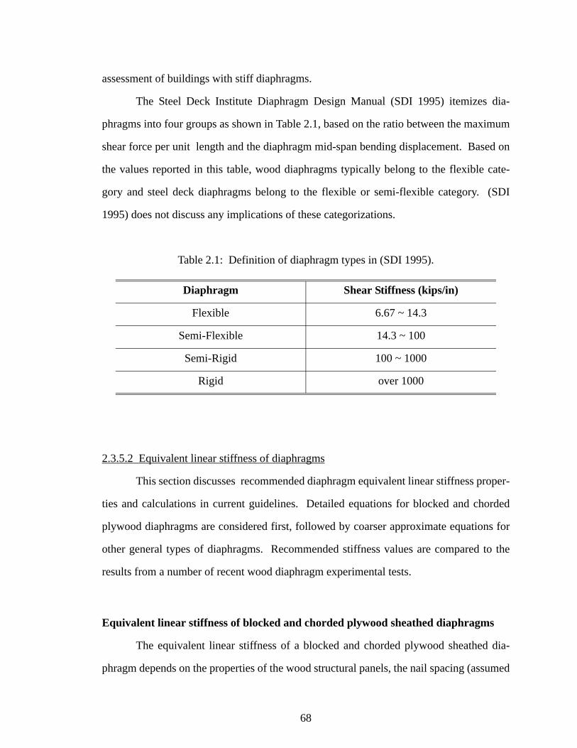
68

assessment of buildings with stiff diaphragms.

The Steel Deck Institute Diaphragm Design Manual (SDI 1995) itemizes dia-

phragms into four groups as shown in Table 2.1, based on the ratio between the maximum

shear force per unit length and the diaphragm mid-span bending displacement. Based on

the values reported in this table, wood diaphragms typically belong to the flexible cate-

gory and steel deck diaphragms belong to the flexible or semi-flexible category. (SDI

1995) does not discuss any implications of these categorizations.

Table 2.1: Definition of diaphragm types in (SDI 1995).

2.3.5.2 Equivalent linear stiffness of diaphragms

This section discusses recommended diaphragm equivalent linear stiffness proper-

ties and calculations in current guidelines. Detailed equations for blocked and chorded

plywood diaphragms are considered first, followed by coarser approximate equations for

other general types of diaphragms. Recommended stiffness values are compared to the

results from a number of recent wood diaphragm experimental tests.

Equivalent linear stiffness of blocked and chorded plywood sheathed diaphragms

The equivalent linear stiffness of a blocked and chorded plywood sheathed dia-

phragm depends on the properties of the wood structural panels, the nail spacing (assumed

Diaphragm Shear Stiffness (kips/in)

Flexible 6.67 ~ 14.3

Semi-Flexible 14.3 ~ 100

Semi-Rigid 100 ~ 1000

Rigid over 1000

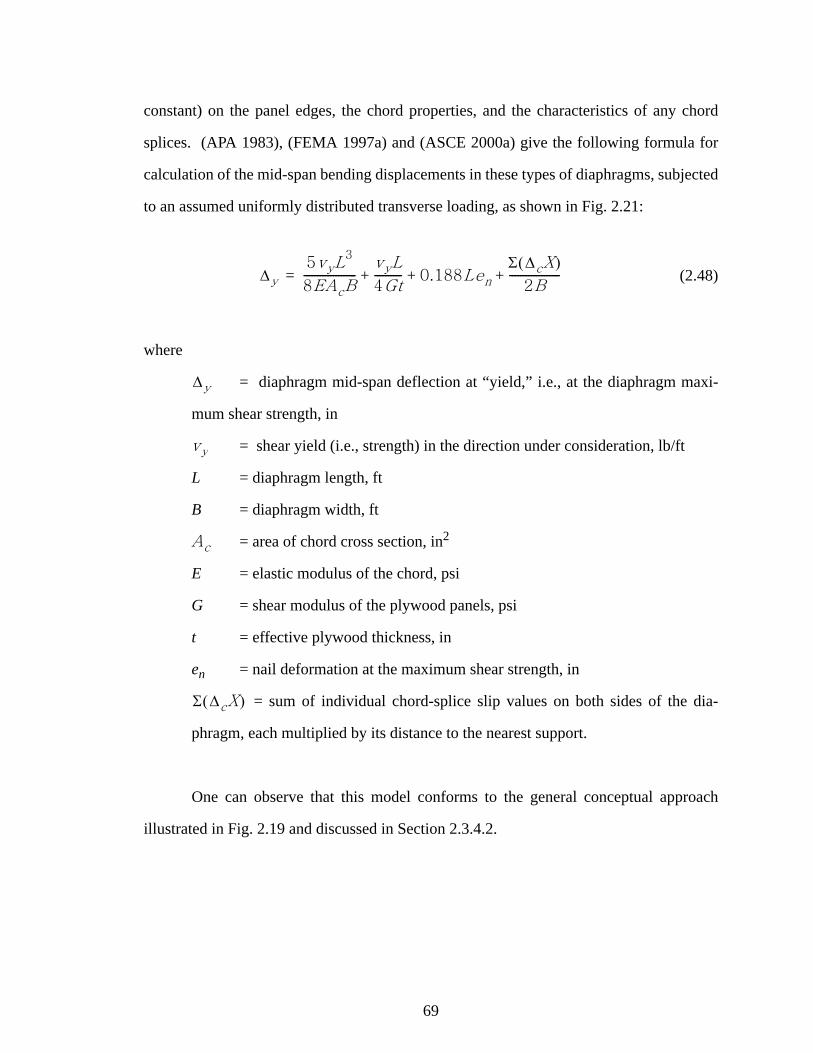
69

constant) on the panel edges, the chord properties, and the characteristics of any chord

splices. (APA 1983), (FEMA 1997a) and (ASCE 2000a) give the following formula for

calculation of the mid-span bending displacements in these types of diaphragms, subjected

to an assumed uniformly distributed transverse loading, as shown in Fig. 2.21:

(2.48)

where

= diaphragm mid-span deflection at “yield,” i.e., at the diaphragm maxi-

mum shear strength, in

= shear yield (i.e., strength) in the direction under consideration, lb/ft

L = diaphragm length, ft

B = diaphragm width, ft

= area of chord cross section, in2

E = elastic modulus of the chord, psi

G = shear modulus of the plywood panels, psi

t = effective plywood thickness, in

en = nail deformation at the maximum shear strength, in

= sum of individual chord-splice slip values on both sides of the dia-

phragm, each multiplied by its distance to the nearest support.

One can observe that this model conforms to the general conceptual approach

illustrated in Fig. 2.19 and discussed in Section 2.3.4.2.

∆y

5vyL3

8EAcB--------------------

vyL

4Gt---------- 0.188Len

Σ ∆cX( )2B

-------------------+ + +=

∆y

vy

Ac

Σ ∆cX( )

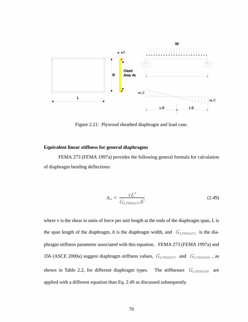
70

Figure 2.21: Plywood sheathed diaphragm and load case.

Equivalent linear stiffness for general diaphragms

FEMA 273 (FEMA 1997a) provides the following general formula for calculation

of diaphragm bending deflections:

(2.49)

where v is the shear in units of force per unit length at the ends of the diaphragm span, L is

the span length of the diaphragm, b is the diaphragm width, and is the dia-

phragm stiffness parameter associated with this equation. FEMA 273 (FEMA 1997a) and

356 (ASCE 2000a) suggest diaphragm stiffness values, and , as

shown in Table 2.2, for different diaphragm types. The stiffnesses are

applied with a different equation than Eq. 2.49 as discussed subsequently.

B

t

ChordArea: Ac

w

L /2

wL /2

wL /2

L /2

∆dvL4

Gd_FEMA273b3

-------------------------------=

Gd_FEMA273

Gd_FEMA273 Gd_FEMA356

Gd_FEMA356

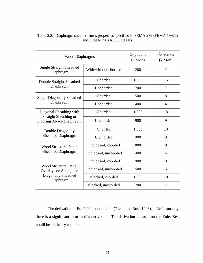
71

Table 2.2: Diaphragm shear stiffness properties specified in FEMA 273 (FEMA 1997a) and FEMA 356 (ASCE 2000a).

The derivation of Eq. 2.49 is outlined in (Tissel and Rose 1993). Unfortunately,

there is a significant error in this derivation. The derivation is based on the Euler-Ber-

noulli beam theory equation

Wood Diaphragms(kips/in) (kips/in)

Single Straight Sheathed Diaphragm With/without chorded 200 2

Double Straight Sheathed Diaphragm

Chorded 1,500 15

Unchorded 700 7

Single Diagonally Sheathed Diaphragm

Chorded 500 8

Unchorded 400 4

Diagonal Sheathing with Straight Sheathing or

Flooring Above Diaphragm

Chorded 1,800 18

Unchorded 900 9

Double Diagonally Sheathed Diaphragm

Chorded 1,800 18

Unchorded 900 9

Wood Structural Panel Sheathed Diaphragm

Unblocked, chorded 800 8

Unblocked, unchorded 400 4

Wood Structural Panel Overlays on Straight or Diagonally Sheathed

Diaphragm

Unblocked, chorded 900 9

Unblocked, unchorded 500 5

Blocked, chorded 1,800 18

Blocked, unchorded 700 7

Gd_FEMA273 Gd_FEMA356

72

(2.50)

in which shear deformations are assumed to be negligible, and where w is an equivalent

uniformly distributed load, L is the diaphragm span, and EI is the diaphragm flexural

rigidity. After substitution of and , where W

is the total lateral load transmitted by the diaphragm, and t is the diaphragm equivalent

thickness (in concept, this is the approach taken in (Tissel and Rose 1993)), this equation

may be expressed as:

(2.51)

where is the appropriate stiffness term associated with this "corrected" equa-

tion, which would of course be different than the reported values in FEMA 273. In other

words, based on the approach taken by (Tissel et al. 1993), the diaphragm bending dis-

placement should be a function of , not . The form of Eq. 2.49 results

from an error in the substitution of the terms. Nevertheless, it is important to emphasize

that neither of these equations should be taken too literally. In other words, Eq. 2.49 (or

alternatively Eq. 2.51) is applied to estimate the deflections in a wide variety of diaphragm

types, many of which are either dominated by shearing deformations or in which, strictly

speaking, Euler-Bernouli beam theory does not apply (Kim and White 2001).

The values of were specified based on limited test data and expert

judgment. Nevertheless, the form of Eq. 2.49 developed in (Tissel et al 1993) is derived

erroneously, and to the knowledge of the authors, has no rational basis. This causes prob-

∆d5wL4

384EI-----------------=

w W L⁄ 2v b L⁄( )= = I tb3( ) 12⁄=

∆dvL3

3.2Etb2--------------------- vL3

Gd_FEMA273b2

-------------------------------= =

Gd_FEMA273

L3 b2⁄ L4 b3⁄

Gd_FEMA273

73

lems when Eq. 2.49 is applied to diaphragms with varying aspect ratios L/b. The greatest

difficulty is when the results of diaphragm tests that have typically been conducted at val-

ues of L/b = 3 (or at similar values) are extended to diaphragms having a small aspect

ratio, say L/b = 1 (which is not uncommon in masonry buildings). These problems will be

explained subsequently, after discussion of a new equation for calculation of diaphragm

deflections, specified in FEMA 356 (ASCE 2000a).

FEMA 356 gives the following equation for calculation of deflections in general

diaphragms:

(2.52)

where is an appropriate specified diaphragm stiffness for use with this equa-

tion (see Table 2.2). Equation 2.52 is based on a shear deformable beam theory in which

the shear deformations are assumed to dominate the response of the system to the extent

such that the contributions from the chord flexibility to the diaphragm deflections (if a

chord exists) may be neglected. In other words, in Eq. 2.52, the flexural rigidity EI is

assumed to be infinite (i.e., the chords are assumed to be rigid). This is in contrast to Eq.

2.51, in which the shear flexibility of the diaphragm is assumed to be zero, and thus the

diaphragm deflections are assumed to come entirely from bending deformations. In the

view of the authors, Eq. 2.52 is a more appropriate equation for calculation of diaphragm

deflections in masonry building systems, since as noted previously, shear deformations are

typically the major contributor to the diaphragm flexibility in these systems.

Comparison to experimental results

Peralta et al. (2001) report recent test results for several representative wood floor

diaphragms. It is interesting to consider how the recommended equivalent linear (i.e.,

∆dvL

2Gd_FEMA356

-----------------------------=

Gd_FEMA356

74

secant) stiffness values from these tests compare to the current values as

well as the initial tangent stiffness values from these tests. Table 2.3 shows these compar-

isons in the context of Eq. 2.52. One should note that the secant stiffness properties rec-

ommended by Peralta et al. (2001) are based on the shear force and mid-span deflection at

the end of the first branch of a bilinear representation of the backbone curve. Peralta et al.

(2001) express the deflection at this point as

(2.53)

where Vy is the actuator force at the middle of the diaphragm (the diaphragms were loaded

by a concentrated force at their mid-span). By equating this expression to Eq. 2.52, rec-

ognizing that vy = Vy/2b, and noting that L/b = 2 for the diaphragms tested in this research,

the appropriate Gd values in the context of Eq. 2.52 are simply K/2.

With the exception of their tongue and groove single straight-sheathed diaphragm

test, the secant stiffnesses in Peralta et al. (2001) are significantly higher than the stiff-

nesses specified in FEMA 356. This might be expected since, based on the derivation of

the equivalent linear stiffness for a plywood diaphragm, the implied stiffness values in

FEMA 356 are secant values to a larger maximum strength level. Furthermore, as would

be expected, the diaphragm initial stiffnesses are significantly higher than the recom-

mended design secant stiffness values.

Peralta et al. (2000) calculate their recommended secant stiffness values based on a

bilinear representation of the experimental backbone curve, with the second branch set as

a tangent to the backbone curve at large diaphragm displacements (the experimental back-

bone curves were approximately linear in this range), and with the first "secant" branch of

the bilinear representation set to obtain equal area under the experimental and bilinear

backbone curves. All sources of deformation (shear and flexural deformations of the floor

system, deformation of the anchorages at the diaphragm boundaries, etc.) are included

Gd_FEMA356

∆y

Vy

K------=

75

within the stiffness values derived from Peralta’s tests. The reader is referred to (Peralta et

al. 2001) for details of the diaphragm characteristics and test results.

Table 2.3: Comparison of FEMA 356 expected and experimental (Peralta et al. 2001) stiffness values for wood diaphragms.

a. = approximate initial tangent stiffness of back-bone curve from experiment (Peralta et al. 2001) based on Eq. 2.52.

b. = secant stiffness of first branch of a bilinear representation of the backbone curve, determined as defined by (Peralta et al. 2001) based on Eq. 2.52.

c. = diaphragm "yield deflection" divided the diaphragm span length, where yield is defined at the

transition to the second branch of the bilinear representation of the backbone curve (Peralta et al. 2001). d. See Fig. 2.17.

One observation regarding the data in Table 2.3 should be considered by the engi-

neer in applying the FEMA 356 equations. FEMA 356 does not distinguish between dif-

ferent types of straight-sheathed diaphragms. Peralta’s study illustrates the fact that the

stiffness properties of diaphragms categorized as the same type in FEMA 356 may be sig-

nificantly different. The 1x4 in. tongue and groove and 1x6 in. board single straight-

Diaphragm Designation and Typekips/in

a

kips/in

b

kips/inc

1A: Single Straight Sheathed (1x4 in. tongue and groove decking

w/ 2x10 in. joists)2 3.3 1.4 0.0020

MAE-2: Single Straight Sheathed (1x6 in. boards w/ 2x10 in. joists)d 2 10 6.0 0.0022

MAE-2B and 2C: Wood Structural

Panel Overlay on Straight Sheathingd

Unblocked, Unchorded

5 30 24 0.0008

Blocked, Unchorded 7 67 33 0.0008

Gd_FEMA356 Gdi Gd_Secant ∆y L⁄

Gdi

Gd_Secant

∆y L⁄

76

sheathed diaphragms tested in (Peralta et al. 2001) have secant stiffness values of

= 1.4 kips/in and 6.0 kips/in respectively, compared to a recommended value of 2 kips/in

in FEMA 356. Depending on one's perspective, it may be argued that the recommended

FEMA 356 values are a reasonable coarse approximation of the broad range of diaphragm

stiffnesses which may exist for this type of diaphragm in practice, or alternatively, it may

be argued that the FEMA 356 equation predictions may be inaccurate by a significant fac-

tor relative to the physical response.

One attribute of the wood diaphragm responses discussed by Peralta et al. (2000),

similar to the observations from (ABK 1981b) discussed in Section 2.3.4.1, is that the dia-

phragms generally were able to accommodate large deformations without significant deg-

radation of the cyclic response.

2.3.5.3 Recommended diaphragm strengths in current guideline documents

(APA 1997) details a commonly accepted procedure for design of plywood dia-

phragms and presents the effects of openings in the diaphragm and field gluing of ply-

wood sheathing. Table 1 of this report gives recommended design shear strengths for

these diaphragm types, derived from prior test results. It is noted that the allowable shear

values vary from other reports depending on the type of framing, splices, ties, hold-downs

and other connections. It is also noted that the controlling diaphragm shear capacity is

based on the type and spacing of the anchorages at the boundary (APA 1997). Table

2306.3.1 of IBC 2000 (ICC 2000) gives recommended design shear strengths for new

plywood sheathed floors or roofs with blocking at panel edges. Sections 8.6.8 and 8.3.2.5

of FEMA356 refer to the yield capacity of wood structural panel diaphragms, but do not

provide specific values for these strengths.

Table 2.4 summarizes recommended diaphragm shear strengths vy from (ABK

1984) and Table 2.5 gives recommended strength values for a number of general dia-

Gd_Secant

77

phragm types from FEMA 356 (ASCE 2000a).

Table 2.4: Diaphragm strengths from (ABK 1984).

a. with roofing applied on the sheathing or a single layer of tongue and groove sheathing without roofing.b. straight sheathing with plywood overlay.

DescriptionStrength vy

(lb/ft)

Straight sheathing 300a

650b

Unblocked plywood sheathing with roofing applied on the sheathing 400

Diagonal sheathing with roofing applied on the sheathing 750

Double board systems with finish flooring laid over diagonal sheathing or multiple board systems with board edges offset 1,800

Metal roof deck systems designed for minimal lateral load capacity; Metal deck with minimal welding 1,800

Metal roof deck systems designed for lateral load capacity; Metal deck welded for seismic resistance 3,000

78

Table 2.5: Diaphragm strengths vy from FEMA 356 (ASCE 2000a).

a. for single straight sheathing, yield capacity shall be multiplied by 1.5 when built-up roofing is present. The value for stiffness shall not be changed.

2.3.5.4 Calculation of equivalent Ee and Ge values for the proposed diaphragm element

based on recommended code and guideline stiffnesses

This section explains the calculation of the chord and shear modulus values of the

proposed diaphragm element, Ee and Ge, based on stiffnesses reported in code and guide-

line documents. The calculation of these values from specific equations for blocked and

DescriptionStrength vy

(lb/ft)

Single straight sheathinga 120

Double straight sheathing Chorded 600

Unchorded 400

Single Diagonally SheathingChorded 600

Unchorded 420

Diagonal Sheathing with Straight Sheathing or Flooring Above

Chorded 900

Unchorded 625

Double Diagonal SheathingChorded 900

Unchorded 625

Wood Structural Panel Overlays on:Straight or Diagonal Sheathing or Existing Wood

Structural Panel Sheathing

Unblocked, Chorded

450

Unblocked, Unchorded

300

79

chorded plywood diaphragms and metal deck diaphragms are discussed first, followed by

the calculation of these values from general equations for other diaphragm types.

Blocked and chorded plywood diaphragms

Based on Eq. 2.15 and considering a lumped transverse loading at the center of the

diaphragm of W/2 = wL/2 = v, where

W = total load in the direction under consideration, in pounds per foot

w = uniformly distributed force, in pounds per foot

v = maximum shear due to loads in the direction under consideration, in units of

force per unit length

L = diaphragm length, in feet

the shear contribution to the mid-span deflection of an equivalent elastic diaphragm with

uniform shear properties throughout may be written as

(2.54)

where Ge is the equivalent elastic shear stiffness. By equating Eq. 2.54 to the shear contri-

bution to the deflection in Eq. 2.48, i.e.,

(2.55)

(where all the terms are expressed in units of lbs and in) the equivalent shear modulus for

a plywood diaphragm can be derived as

(2.56)

∆svL

4Get-------------=

vL4Get------------- vL

4Gt---------- 0.188Len+=

GevG

v 0.0627enGt+-------------------------------------------=

80

Similarly, an equivalent elastic chord modulus for the proposed diaphragm ele-

ment, including the effects of both the chord flexibility as well as chord splice slip, may be

derived by equating Eq. 2.18 to the flexural contributions to the displacement in Eq. 2.48.

This gives

(2.57)

Metal deck

Due to their corrugated profile, steel deck sections exhibit anisotropic behavior

(Easterling 1994b). Also, the shear stiffness of these types of diaphragms is influenced

significantly by distortion of the deck profile under the action of shear forces. (SDI 1995)

bases its suggested equations for diaphragm shear stiffness on a more fundamental test

than considered in the previously discussed wood diaphragm research. The test configura-

tion considered by (SDI 1995) is illustrated in Fig. 2.22. If the proposed diaphragm ele-

ment is applied to the analysis of this test, the shear deflection is obtained as

Figure 2.22: Schematic layout for metal deck diaphragm.

Ee5vEL3

5vL3

48Σ ∆cX( )EAc+-----------------------------------------------------------=

L

∆

B

P

P

R R

81

(2.58)

(SDI 1995) gives a similar equation for this deflection, and defines an equivalent shear

modulus of the diaphragm, considering the effects of corrugations, warping relaxation,

and discrete connections at panel side laps as

(2.59)

where:

E = modulus of elasticity, kips/in2

= Poisson’s ratio, 0.3

= warping constant

S = girth of corrugation per rib, in

C = connector slip parameter

d = corrugation pitch, in

The reader is referred to (SDI 1995) for specific values of these constants.

The equivalent stiffness for the proposed diaphragm element is obtained simply as Ge =

G’.

Metal deck with concrete topping

For diaphragms with concrete topping over a corrugated steel deck, the shear

capacity increases proportionally with the added concrete. In addition, the concrete top-

∆svLGet---------=

G'′ E

2 1 ν+( )Sd--- Dn C+ +

--------------------------------------------------=

ν

Dn

82

ping eliminates the panel end warping effect for loads within the design range (SDI 1995).

Thus, the warping constant term of Eq. 2.59 approaches zero. Finally, the total effective

modulus is increased by adding second term in Eq. 2.60:

(2.60)

where

= concrete cover depth

= concrete compressive strength, psi

General diaphragms

The equivalent elastic stiffnesses Ge and Ee for the proposed diaphragm element

may be determined for general diaphragms from the FEMA 356 (ASCE 2000a) stiffness

values as follows. Based on the idealization of the diaphragm as being rigid

in flexure and deformable only in shear (see the discussion of Eq. 2.52), Ee may be set

effectively to infinity. That is, the flexural contributions to the diaphragm flexibility coef-

ficients are taken as zero. Subsequently, Eq. 2.54 may be equated to Eq. 2.52 to obtain

(2.61)

Similarly, again assuming that the diaphragm response is dominated by shearing

type deformations, the equivalent shear modulus for the proposed diaphragm element cor-

responding to the FEMA 273 (FEMA 1997a) general diaphragm stiffness equation is

(2.62)

GeE

2 1 ν+( ) Sd---× C+

------------------------------------------3.5dc fc′( )0.7

t----------------------------------+=

dc

fc′

Gd_FEMA356

Ge

Gd_FEMA356

2t-------------------------------=

Ge

Gd_FEMA273B3

4L3t

--------------------------------------=

83

2.3.5.5 Example calculations

In this section, the relative contribution of bending and shear deformations to the

deflections in representative plywood and steel deck diaphragms are examined. The pur-

pose of this study is to investigate when the bending deformations may be neglected. The

following assumptions are invoked: (1) The area of the chord member is constant in all the

studies. (2) Only the chord member at the outer edge of diaphragm is considered in calcu-

lating the bending stiffness, i.e, the potential contribution of the walls to the chord stiff-

ness is not included. (3) The stiffness of walls subjected to out-of-plane bending is

neglected. (4) The lateral load is uniformly distributed.

Wood Diaphragm

Consider the plywood diaphragm from (Tissell and Elliot 1983) shown in Fig.

2.23. Various properties of this diaphragm required for the diaphragm displacement calcu-

lations are shown in Table 2.6. The bending and shear contributions to the displacements

for this diaphragm are determined from the fundamental equation

(2.63)

where Ee and Ge are determined from Eqs. 2.56 and 2.57, I is taken as AcB2/2, and Aw =

Bt. The first term in Eq. 2.63 is the flexural or bending contribution to the displacement

and the second term is the shear contribution to the displacement . The following

assumptions from (Tissell and Elliot 1983) are invoked to determine the chord splice con-

tribution to Ee along with Eq. 2.57:

∆ 5wL4

384EeI-------------------- αs

wL2

8GeAw

-------------------+=

∆b ∆s

84

• Each chord of the diaphragm in Fig. 2.23 is composed of four 12 ft long segments.

Therefore, there are three internal splices in each segment.

• Tension chord: The splice slip is assumed to be 0.011 in for both of the outer

splices and 0.015 in for the center splice.

• Compression chord: The splice slip is assumed to be 0.002 inches at all of the

splice locations.

In the discussions below, the aspect ratio of this diaphragm L/B is varied from 1 to 5 at

increments of one. For L/B values other than the value of three for the diaphragm shown

in Fig. 2.23, the chords are still assumed to be composed of 12 ft long segments. The

splice slip values are taken as described above, with the tension chord splice slips taken as

0.011 in only at the outer splices and 0.015 in for all interior splices. The tension chord

splice slip is taken as 0.011 in for L/B = 2.

Based Eq. 2.63, one can write

(2.64)

and

(2.65)

Table 2.7 shows the corresponding computed total displacement , shear contribution to

this total displacement , the bending contribution , and the ratios and for

this diaphragm if its aspect ratio L/B is varied from 1 to 5. Fig. 2.24 shows the plot of the

corresponding total displacement, and the flexural and shear contributions to this displace-

ment as a function of the diaphragm aspect ratio. As the aspect ratio increases from 1 to 5,

∆c

∆c

∆b

∆s

------ 524-------

GeAw

EeAc

---------------⎝ ⎠⎛ ⎞ L

B----⎝ ⎠

⎛ ⎞ 2=

∆S

∆------ 1

1524-------

GeAw

EeAc

--------------- LB----⎝ ⎠

⎛ ⎞ 2+

-----------------------------------------------=

∆

∆s ∆b

∆s

∆------

∆b

∆------

85

the ratio of increases from 9% to 32%. One can observe that even at an aspect ratio of

3, the contribution of the chord flexural deformations to the total diaphragm bending dis-

placement is less than 20%. If the structural walls also provide some contribution to the

chord stiffness, the flexural contribution to the total displacement is reduced further.

Figure 2.23: Framing details and panel layout for a representative plywood diaphragm (Tissell and Elliott 1983).

∆b

∆------

86

Table 2.6: Values for example plywood diaphragm deflection calculations (APA 1983).

Variable Value

Shear in the direction under consider-ation vy 35.42 lb/in

Length of Diaphragm L 576 inch ( L/B = 3)

Width of Diaphragm B 192 inch

Young’s Modulus (Chord Member) E psi

Shear Modulus (Panel) G psi

Area of Chord Cross Section 32.375

Effective Plywood Thickness t 0.535 inch

Nail Deformation en

Shear Coefficient 1.0

1.7x107

9.0x104

Ac in2

v1538--------------⎝ ⎠

⎛ ⎞ 3.276

αs

87

Table 2.7: Total displacements, shear and bending contributions to the total displacements and ratios of these contributions to the total for a representative wood diaphragm.

Figure 2.24: Example plywood diaphragm displacements.

Steel deck diaphragm

Consider the steel deck diaphragm from (SDI 1995) shown in Fig. 2.25. Various

properties of this diaphragm required for the displacement calculations are shown in Table

Diaphragm aspect ratio

(L/B)

Displacement (in)

1 0.088 0.080 0.008 0.907 0.093

2 0.183 0.160 0.024 0.871 0.129

3 0.294 0.239 0.055 0.814 0.186

4 0.423 0.319 0.103 0.756 0.244

5 0.582 0.399 0.183 0.685 0.315

∆ ∆s ∆b∆s

∆------

∆b

∆------

0

0.10.2

0.30.4

0.50.6

0.7

1 2 3 4 5L/B

Dis

plac

emen

t (in

ch) Total displacement

Shear contributionFlexural contribution

88

2.8. The displacements of this diaphragm may also be calculated from Eq. 2.63. Table 2.9

shows the corresponding computed total displacement , the bending contribution in this

total displacement , the shear contribution , and the ratio of and for this

diaphragm if its aspect ratio is varied from 1 to 5. Fig. 2.26 shows the plot of the corre-

sponding total displacement, and the flexural contribution and shear contributions to this

displacement as function of steel deck diaphragm aspect ratio.

Table 2.8: Values for calculation of deflections in an example steel deck diaphragm (SDI 1995).

Variable Initial Value

Uniform Lateral Load w 16.67 lb/in

Length of Diaphragm L 120 ft ( L/B = 3)

Width of Diaphragm B 40 ft

Young’s Modulus (Joist Member) E 29,500 ksi

Effective Shear Modulus Ge 1000 ksi

Section Area of Joist Member 10

Thickness t 0.03 inch

Shear Coefficient 1.0

∆

∆b ∆s

∆s

∆------

∆b

∆------

Ac in2

αs

89

Figure 2.25: Representative steel deck diaphragm (SDI 1995).

Table 2.9: Total displacements, shear and bending contributions to the total displacements, and ratios of these contributions to the total for a representative steel deck

diaphragm.

Diaphragm aspect ratio (L/B)

Displacement (inch)

1 0.034 0.034 0.0003 0.991 0.009

2 0.139 0.134 0.005 0.964 0.036

3 0.327 0.300 0.027 0.917 0.083

4 0.62 0.533 0.087 0.860 0.140

5 1.045 0.833 0.212 0.797 0.203

H =

40

ft

10 ft

10 ft

10 ft

10 ftJoists

DiaphragmPanel

L = 120 ft

∆ ∆s ∆b∆s

∆------

∆b

∆------

90

Figure 2.26: Example steel deck diaphragm displacements.

Comparison of two diaphragms

Figure 2.27 compares the ratio of the shear contribution to the displacement to the

total displacement, , for the plywood and steel deck diaphragms (calculated per Eq.

2.65). The value of is constant for all the aspect ratios in the steel deck dia-

phragm. However, because of the assumption of chord splices at every 12 ft in the ply-

wood diaphragm, the varies as a function of the aspect ratio in this case.

Figure 2.27 shows that the ratio of is greater than or equal to 0.8 for the steel

deck diaphragm. Because of the effects of the chord splices on the chord flexibility, is

as low as 0.69 for an aspect ratio of 5 in the wood diaphragm. However, as noted previ-

ously, is greater than 0.8 for L/B < 3 in this diaphragm.

Based on the above results, one can conclude that in many practical cases, it is suf-

ficient to neglect the contributions from the chord flexibility altogether in approximating

the diaphragm responses. That is, in many cases, the diaphragm response can be idealized

as rigid with respect to the flexure and only the diaphragm shear deformations need be

considered in determining the bending and shear raking displacements. It is again noted

that this idealization is invoked in the general FEMA 356 equation for the diaphragm

0

0.2

0.4

0.6

0.8

1

1.2

1 2 3 4 5L/B

Dis

plac

emen

t (in

ch) Total displacement

Shear contributionFlexural contribution

∆s

∆------

GeAw

EeAc

---------------⎝ ⎠⎛ ⎞

GeAw

EeAc

---------------⎝ ⎠⎛ ⎞

∆s

∆------

∆s

∆------

∆s

∆------

91

bending displacements, Eq. 2.52.

,

Figure 2.27: Comparison of deflection ratios.

2.4 Wall models

As discussed in Chapter I, the proposed modeling approach uses two degree-of-

freedom shear spring elements within each story to analyze the wall responses. Each in-

plane wall is represented by a single degree of freedom at each story level. These degrees

of freedom are connected by one or more shear springs. A single shear spring element

may be used as shown in Fig. 2.28 (a) if the engineer wishes to characterize the overall

behavior of the wall within a given story using a single hysteretic model. Multiple shear

spring elements as shown in Fig. 2.28 (b) may be connected in parallel to the correspond-

ing story DOFs to track the behavior of each of the wall components directly. In this case,

the overall wall hysteretic response is obtained by summing the responses from each of

the components. In cases where the wall behavior is elastic, or if the engineer can approx-

0.0

0.1

0.2

0.3

0.4

0.5

0.6

0.7

0.8

0.9

1.0

0 0.05 0.1 0.15 0.2 0.25 0.3 0.35 0.4 0.45 0.5

Wood Diaphragm (APA 1983)

Steel Deck Diaphragm (SDI 1995)

92

imate the overall hysteretic response of the wall via a single hysteretic curve, only one ele-

ment is needed per wall.

Figure 2.28: Shear wall element: (a) single shear spring element and (b) multiple shear spring elements.

As noted previously, the primary focus of the current research is on unreinforced

masonry structures. The material properties for calculation of initial elastic wall stiff-

nesses in these types of buildings are discussed in Section 2.4.1. The initial elastic stiff-

ness of each of the in-plane walls is determined in this work using either a finite element

plane stress analysis and a flexibility approach, or by simplified strength of materials

approaches. These calculations are presented in Section 2.4.2. The overall wall strength

is determined by summing the strengths determined from each of the wall components.

These strength calculations are discussed in Section 2.4.3.

As noted above, the overall wall hysteretic response may be approximated by a

single hysteretic curve, based generally on judgment, or by the use of multiple wall ele-

ments, connected in parallel to the corresponding story degrees of freedom, each with

their own independent hysteretic model. The hysteretic models that may be utilized for

the walls include the three-parameter model discussed previously with respect to the anal-

U1

U2

1 2 3 4

k1 k2 k3 k4

(a) (b)

93

ysis of the diaphragm responses, as well as a rocking model and a bed-joint sliding model.

The three-parameter model is useful for representing the behavior of walls or piers that

exhibit a diagonal tension mode of failure.

Section 2.4.4 discusses the inclusion of flange effects from the out-of-plane walls

in the modeling of in-plane walls. Section 2.4.5 discusses a special case of the basic pier

rocking models addressed earlier in Section 2.4.3: the modeling of piers that fail by a mul-

tiple story rocking mechanism. Section 2.4.6 addresses the calculation of individual com-

ponent stiffnesses when an in-plane wall is represented by multiple parallel spring

elements. Section 2.4.7 discusses the modeling of out-of-plane walls.

2.4.1 Wall material properties in code and guideline documents

The behavior of masonry walls is more complex than that of concrete shear walls

(Shing 1998). This is due to the nonhomogeneous nature of unreinforced masonry,

involving the interaction of the constituent materials, i.e., brick, mortar, and grout, The

influence of mortar joints as weak planes is a significant feature that is not present in con-

crete. Masonry walls do not fail immediately after cracks develop. They can possess a

gradual softening until the ultimate limit state is achieved, and they can be deformed con-

siderably (Abrams 1992).

A representative masonry strain-strain response curve from a compression prism

test (MSJC 1999c) is shown in Fig. 2.29. This figure shows one definition of the elastic

modulus for masonry in compression, Em. The commentary to ACI 530-99 (MSJC

1999b) explains that the elastic modulus in compression of masonry has been traditionally

taken as 1000 , but indicates that lower values are more typical. FEMA 356 (ASCE

2000a) suggests

(2.66)

fm′

Em 550 fm′×=

94

as an expected value for the elastic modulus of masonry in compression, where is

the masonry compressive strength.

Figure 2.29: Compressive stress-strain response of masonry (MSJC 1999b).

Table 2.10 gives expected values for suggested by FEMA 273 (FEMA 1997),

and the corresponding values for Em for masonry in good, fair and poor condition.

Table 2.10: Summary of elastic modulus with compressive strength in FEMA 273 (FEMA 1997) and FEMA 356 (ASCE 2000a).

Condition (FEMA273 and FEMA 356 Masonry compressive strength)

(FEMA 273 Masonry elastic modulus)

Good < 900 psi < 495 ksi

Fair < 600 psi < 330 ksi

Poor < 300 psi < 165 ksi

fm′

fm′

fm′ Em

95

ACI 530-99 (MSJC 1999a) suggests the following expected values for Em:

for clay masonry (2.67)

for cement masonry (2.68)

and IBC 2000 (ICC 2000) suggests a design value of

3,000 ksi max. for clay, shale, or cement unit masonry (2.69)

The ACI 530-99 (MSJC 1999a) and UBC 1997 (ICBO 1997) codes specify the

modulus of elasticity of grout as

(2.70)

where is the grout compressive strength.

Common practice is to use the Em value from one of the above approaches as the

elastic modulus, along with an effective wall thickness, for structural analysis. FEMA273,

ACI 530-99, and UBC 1997 suggest that the shear modulus of unreinforced masonry may

be taken as

(2.71)

This corresponds to a Poisson’s ratio of 0.25.

Em 700 fm′×=

Em 900 fm′×=

Em 750 fm′×=

Eg 500 fg×=

fg

Gm 0.4Em=

96

2.4.2 Determination of wall initial elastic stiffness

The lateral displacement of a single shear wall without openings may be calculated

using simple flexural theory. However, openings are often introduced in shear walls,

thereby reducing their effectiveness and altering their deformation characteristics. Simpli-

fied methods that give reliable estimates for the lateral stiffness of perforated shear walls

are not available at this time (December 2002). Given an accurate characterization of the

material stiffness and effective thickness, a flexibility approach based on the use of plane-

stress finite element analysis has been shown by Tena-Colunga and Abrams (1992a) to

provide a significant improvement in the overall accuracy of the analysis relative to typi-

cal simplified methods.

The next subsection discusses two typical simplified methods for calculating elas-

tic wall stiffnesses. This is followed by an explanation of the above flexibility approach

and a comparison of the results from this approach to those of the simplified calculations

for an example wall.

2.4.2.1 Initial stiffness calculation based on strength of materials type analysis

Schneider and Dickey (1994) suggest several simplified methods for the elastic

stiffness of single-story masonry walls. These models are explained in the following

subsections using the perforated wall shown in Fig. 2.30.

Figure 2.30: Example perforated wall (Schneider and Dickey 1994).

P

41

2

3

6

5

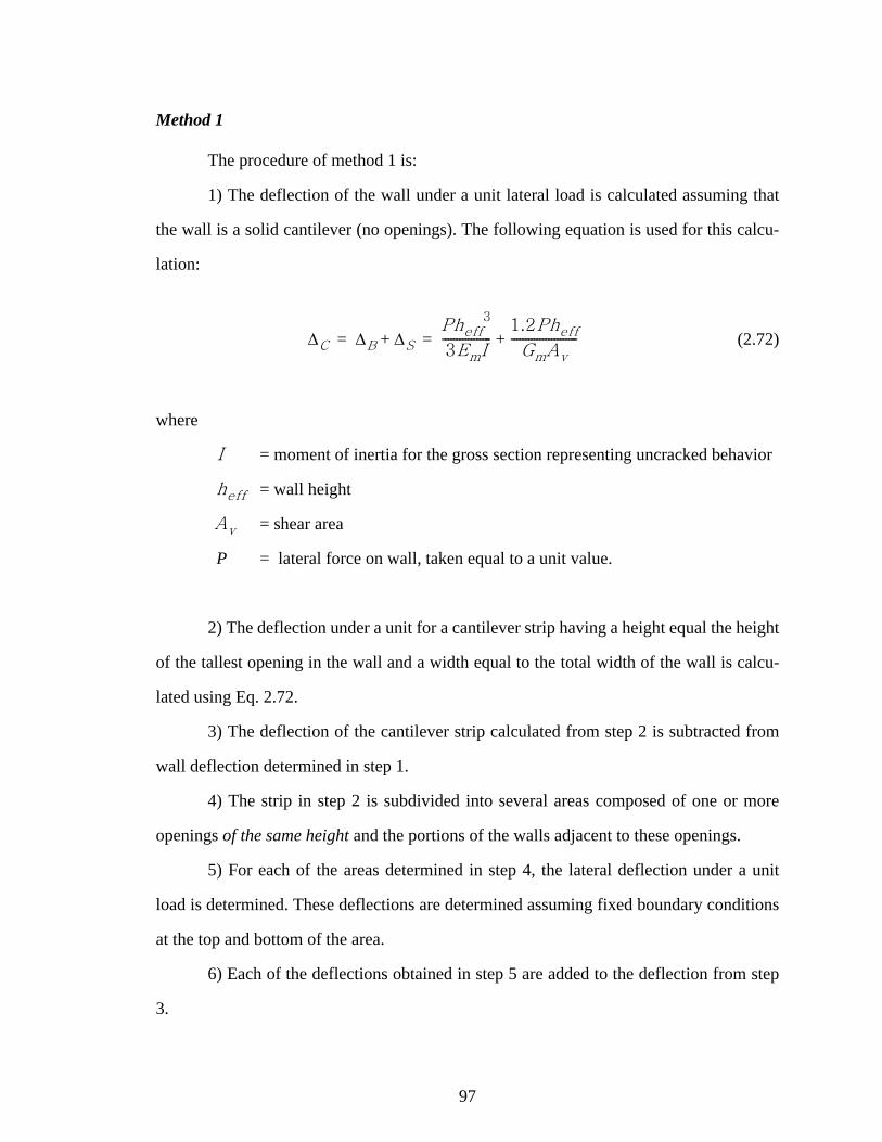
97

Method 1

The procedure of method 1 is:

1) The deflection of the wall under a unit lateral load is calculated assuming that

the wall is a solid cantilever (no openings). The following equation is used for this calcu-

lation:

(2.72)

where

= moment of inertia for the gross section representing uncracked behavior

= wall height

= shear area

P = lateral force on wall, taken equal to a unit value.

2) The deflection under a unit for a cantilever strip having a height equal the height

of the tallest opening in the wall and a width equal to the total width of the wall is calcu-

lated using Eq. 2.72.

3) The deflection of the cantilever strip calculated from step 2 is subtracted from

wall deflection determined in step 1.

4) The strip in step 2 is subdivided into several areas composed of one or more

openings of the same height and the portions of the walls adjacent to these openings.

5) For each of the areas determined in step 4, the lateral deflection under a unit

load is determined. These deflections are determined assuming fixed boundary conditions

at the top and bottom of the area.

6) Each of the deflections obtained in step 5 are added to the deflection from step

3.

∆C ∆B ∆S+Pheff

3

3EmI-----------------

1.2Pheff

GmAv

-----------------------+= =

I

heff

Av

98

7) The stiffness of the wall is obtained by taking the reciprocal of the displacement

from step 6.

In step 5, the deflections are calculated for each of the wall areas in a fashion simi-

lar to the procedure for the total wall. The deflection is first calculated assuming that the

wall is solid within the area under consideration (no openings). Second, the deflection of a

strip having a height equal to the height of the openings in this area is subtracted from the

above. Finally, the deflection of each of the piers of height equal to the height of the open-

ings is calculated an added to the above result. The deflection equation used in these area

calculations is

(2.73)

where P is again taken as a unit load, and the dimensional parameters correspond to the

area under consideration.

Method 2

The stiffness using method 2 is determined simply by summing the stiffnesses of

the individual piers between the openings within the wall, i.e.,

for (2.74)

where the individual pier stiffnesses ki are obtained from Eq. 2.73.

2.4.2.2 Initial stiffness by flexibility approach, using plane stress finite element analysis

The calculation of the lateral stiffness by the flexibility approach can be explained

using the representative two-story perforated wall shown in Fig. 2.31. The general proce-

∆F ∆B ∆S+Pheff

3

12EmI-----------------

1.2Pheff

GmAv

----------------------- += =

K ki

i 1=

n

∑ 1∆i

-----i 1=

n

∑= = i 1 2 3 … n, , , ,=

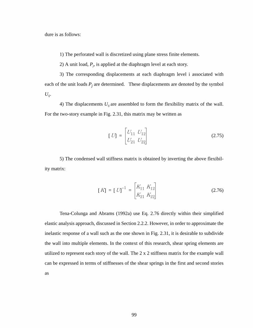
99

dure is as follows:

1) The perforated wall is discretized using plane stress finite elements.

2) A unit load, Pj, is applied at the diaphragm level at each story.

3) The corresponding displacements at each diaphragm level i associated with

each of the unit loads Pj are determined. These displacements are denoted by the symbol

Uij.

4) The displacements Uij are assembled to form the flexibility matrix of the wall.

For the two-story example in Fig. 2.31, this matrix may be written as

(2.75)

5) The condensed wall stiffness matrix is obtained by inverting the above flexibil-

ity matrix:

(2.76)

Tena-Colunga and Abrams (1992a) use Eq. 2.76 directly within their simplified

elastic analysis approach, discussed in Section 2.2.2. However, in order to approximate the

inelastic response of a wall such as the one shown in Fig. 2.31, it is desirable to subdivide

the wall into multiple elements. In the context of this research, shear spring elements are

utilized to represent each story of the wall. The 2 x 2 stiffness matrix for the example wall

can be expressed in terms of stiffnesses of the shear springs in the first and second stories

as

U[ ]U11 U12

U21 U22

=

K[ ] U[ ] 1– K11 K12

K21 K22

= =

100

Figure 2.31: Representation of a perforated cantilever wall (Tena-Colunga and Abrams 1992a).

(2.77)

where K1 and K2 are the stiffnesses of the shear springs within the first and second stories

respectively. The fundamental formulation of this stiffness matrix is illustrated in Fig.

2.32.

Given Eqs. 2.76 and 2.77, the elastic stiffness of the second story is calculated by

equating diagonal coefficients in the second row of the matrices, i.e.,

(2.78)

Once K2 is determined, K1 is calculated by equating the diagonal coefficients in

the first row of the above equations. This gives

(2.79)

U1

U2

P1

U21

U11

P2U22

U12

K[ ]K1 K2+ K– 2

K– 2 K2

=

K2 K22=

K1 K11 K2–=

101

Figure 2.32: Calculation of story stiffness.

A similar approach is employed for walls with more than two stories. The shear

spring stiffnesses are obtained by equating the diagonal coefficients of the stiffness matrix

obtained by plane stress finite element analysis to the corresponding diagonal coefficients

associated with the shear spring idealization.

The above procedure of course gives only an approximation of the elastic stiffness

matrix for the complete wall obtained from the plane stress analysis. The diagonal coeffi-

cients obtained from the plane stress analysis are matched exactly, but the off-diagonal

stiffness terms are generally not the same. Also, the elastic stiffness from the plane stress

analysis is generally full. That is, all of the story degrees of freedom are coupled. A non-

zero force is produced at any story level i due to a unit deflection at any story level j. How-

ever, only the adjacent story degrees of freedom are coupled using the shear spring ideali-

zation, as illustrated in Fig. 2.32. By equating the diagonal coefficients, a suitable

approximation of the “exact” wall stiffness is obtained that satisfies equilibrium in the

context of the story-by-story shear spring idealization.

2.4.2.3 Comparison of methods

Figure 2.33 shows the plane stress finite element discretization and deformed

geometry for two perforated walls from Schneider and Dickey (1994) and Tena-Colunga

K1

K11

K21 = K2

K12

K22

K2

K1

(a) (b) (c)

102

and Abrams (1992a) (labeled as walls B and C in these references). A four-node plane-

stress element is used for the analysis using ABAQUS Version 5.8 (HKS 1998). The elas-

tic modulus of the wall is taken as Em = 1200ksi, Gm is determined per Eq. 2.71, and the

equivalent wall thickness is taken as 8.5 in. A lateral load of P = 1,000 kips is applied at

the top of the wall. Since this problem involves only a single story, the “exact” stiffness

per the plane stress analysis is used directly within the shear spring idealization. The

deflections predicted by this recommended approach are compared to the corresponding

predictions using Methods 1 and 2 from Section 2.4.2.1 in Table 2.11. Similar results are

reported by Tena-Colunga and Abrams (1992a).

(a) Wall B: Undeformed mesh (b) Wall C: Undeformed mesh

(c) Wall B: Deformed mesh and (d) Wall C: Deformed mesh and minimum principal stress minimum principal stress

Figure 2.33: Perforated walls for the comparison between the simplified and the FEM analysis.

Both of the simplified methods tend to underestimate the lateral deflections in this

problem. Method 1 gives the best predictions of these two approaches for these walls.

The predicted lateral displacements only 0.25 and 0.26 of the values obtained from finite

103

element analysis using Method 2.

Table 2.11: Comparison of the displacement of the perforated cantilever walls by FEM vs. Method I and II (Tena-Colunga and Abrams 1992a).

2.4.3 Wall strength and hysteresis models

The physical behavior of general perforated masonry walls is complex. Many

types of failure are possible and the strength and hysteretic response can vary significantly

as a function of the failure mode. The failure mode can be influenced by the nonhomoge-

neous nature of these wall types. As the lateral force on a wall or pier increases, flexural or

shear cracking - or a combination of both - occurs. Shear failures, i.e., diagonal tension or

bed-joint sliding limit states, are common types of failure of masonry walls (Zhuge 1998).

In this research, simplified equations specified in FEMA 273, FEMA 356 and EC 6 are

adapted to calculate the strength of walls as a whole and of individual wall components.

According to FEMA 274 (FEMA 1997b), four different failure modes can occur in

masonry walls and/or their components: diagonal tension, bed-joint sliding, toe crushing,

and rocking. It is well known that the strength and hysteresis behavior of masonry shear

walls depends predominantly on the length-to-height aspect ratio (L/H) and the amount of

vertical compressive stress overall and within the individual components of the wall.

FEMA 274 categorizes rectangular walls or piers according to L/H as shown in the first

two columns of Table 2.12. The most common modes of failure for each of the categories

are described in the third column of the table. Table 2.13 gives the characterization of the

failure modes adopted in this research based on the combined rules in FEMA 273 (FEMA

WALL FEM (ABAQUS)in

Method 1in

Method 2in

B 0.2832 0.152 0.071

C 0.3483 0.201 0.091

104

1997a) and EC6 (CEN 1995). The categorization of the behavior into two types of diago-

nal tension failure, per EC6, is adopted here. FEMA 273 lists only the four basic failure

modes discussed above.

The behavior of stocky walls (L/H greater than 1.5) is typically governed either by

diagonal tension or bed-joint sliding. The crack pattern associated with diagonal tension

can develop in either a stair-step pattern through the mortar head and bed joints, or along a

straight diagonal path through the masonry units. For taller more slender walls or piers,

the strength and hysteresis behavior is typically governed either by rocking or toe-crush-

ing. As the lateral force approaches to PL/2H, a wall or pier will start to rock about its toe.

Walls and piers with an intermediate aspect ratio (L/H between 1.0 and 1.5) are more apt

to be governed by toe crushing, which occurs after flexural cracks form at the heel of a

wall. Slender walls (L/H < 1.0) loaded by relatively light vertical compressive forces are

typically governed by rocking. Although the above modes of failure (listed also in Table

2.12) are the most common for each of the wall types, in general the strength associated

with each of the five damage models listed in Table 2.13 must be checked. The controlling

damage model is taken as the one that gives the smallest strength.

Table 2.12: Categorization of rectangular masonry walls and piers (FEMA 1997b).

Wall Type L/H Typical Failure Mode

Stocky walls > 1.5 Diagonal tension cracking or bed-joint sliding

Moderate walls > 1.0 and < 1.5 Rocking or toe crushing

Slender walls < 1.0 Rocking

105

Table 2.13: Characterization of failure modes in rectangular masonry walls and piers, adapted from (FEMA 1997b) and (CEN 1995).

Simple hysteresis models can be constructed to represent bed-joint sliding and

rocking, since experimental tests show little stiffness degradation, strength deterioration or

pinching associated with these limit states. However, the hysteretic responses associated

with diagonal tension and toe crushing are not well established at the present time. The

three parameter model discussed in Section 2.3.4.1 is expected to give a reasonable

approximation of hysteresis response for walls that fail by diagonal tension or toe crush-

ing. This model captures the essential characteristics associated with these modes of fail-

ure, i.e., stiffness degradation, strength deterioration and pinching.

Recommendations are provided for calculation of the strength and hysteresis of

rectangular walls and piers in the following subsections. The recommended strength equa-

tions are adapted from FEMA273 (FEMA 1997a) and EC6 (CEN 1995). For purposes of

discussion, the recommendations are organized using the damage index numbers shown in

the last column of Table 2.13. Generally, the total shear strength of a perforated wall is

obtained by summing the strengths from its components.

Failure Mode Description of Damage Damage Model Index

Diagonal tension crack

Stair-step pattern 1

Straight diagonal pattern 2

Bed-joint sliding Sliding at one or several bed joints 3

Toe crushing Flexural cracking at the heel of the wall and crushing at the toe 4

Rocking

Flexural cracks along a bed joint near the base of the wall

5Bed-joint crack will develop across almost all of the wall base

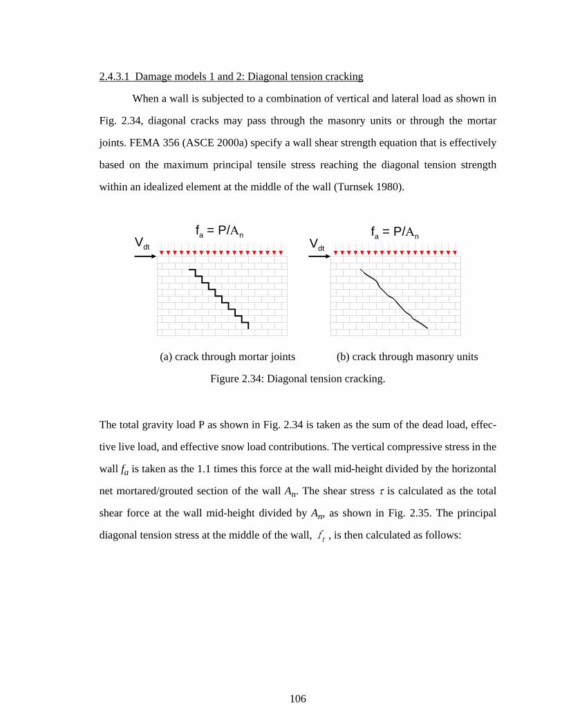
106

2.4.3.1 Damage models 1 and 2: Diagonal tension cracking

When a wall is subjected to a combination of vertical and lateral load as shown in

Fig. 2.34, diagonal cracks may pass through the masonry units or through the mortar

joints. FEMA 356 (ASCE 2000a) specify a wall shear strength equation that is effectively

based on the maximum principal tensile stress reaching the diagonal tension strength

within an idealized element at the middle of the wall (Turnsek 1980).

(a) crack through mortar joints (b) crack through masonry units

Figure 2.34: Diagonal tension cracking.

The total gravity load P as shown in Fig. 2.34 is taken as the sum of the dead load, effec-

tive live load, and effective snow load contributions. The vertical compressive stress in the

wall fa is taken as the 1.1 times this force at the wall mid-height divided by the horizontal

net mortared/grouted section of the wall An. The shear stress τ is calculated as the total

shear force at the wall mid-height divided by An, as shown in Fig. 2.35. The principal

diagonal tension stress at the middle of the wall, , is then calculated as follows:

fa = P/Αn fa = P/ΑnVdt Vdt

ft

107

Figure 2.35: Principal stress for unit area.

(2.80)

where

= shear stress distribution factor, which depends on the geometry of

wall

= height from the base of the wall to the resultant of the applied lateral

force

This equation is obtained from Mohr’s circle, except that the shear stress is modi-

fied by the shear stress distribution factor b. Equation 2.80 was developed originally by

(Turnsek 1980) and is also discussed in (Tomazevic 1999).

By equating ft to the lower-bound diagonal tension strength of the masonry f ’dt and

solving Eq. 2.80 for τ, the lateral shear resistance may be expressed as

(2.81)

where, = lateral strength limited by diagonal tension

ττ

τ = Vdt / Αn

τ

fa = P/Αn

ft

ft

fa

ft

fa

2----⎝ ⎠

⎛ ⎞2

bτ( )2+fa

2----–=

bheff

L----------=

heff

Vdt

fdt′AnL

heff

-------------------- 1fa

fdt′--------+=

Vdt

108

FEMA 356 do not recommend any specific values for f ’dt, but state, “Substitution

of the bed-joint shear strength, vme, for the diagonal tension strength f ’dt in Equation (7-5)

[Equation 2.81 in the above] shall be permitted.” The bed-joint shear strength is discussed

in the next subsection. FEMA 356 state that Eq. 2.81 is applicable only for 0.67 < <

1.00. No recommendations are provided for walls or components that do not meet these

limits.

As noted previously, EC6 considers two different potential diagonal tension failure

modes for URM, denoted by indices 1 and 2 in Table 2.13. The lateral shear resistance

for damage model 1 (which involves stair-step diagonal tension cracking) is expressed in

EC6 as (Tomazevic 1999)

(2.82)

where

= shear strength under zero compression stress

= slip coefficient, assumed equal to 0.75

= vertical design compression stress

= material partial safety factor

= length of the compressed part of the wall

This equation is applied in this research by taking = 1 and = fa.

The shear resistance for damage model 2 (a straight diagonal tension crack through

the mortar and masonry units) is calculated in EC6 using Eq. 2.81, but the nominal

strength is divided by the partial safety factor , and is multiplied by 0.9 if the hysteretic

response is idealized as bilinear. The FEMA 356 equation is used directly for damage

model 2 in this research.

Lheff

----------

Vdt

vto µcσd+( )tLc

γ-----------------------------------------=

vto

µc

σd

γ

Lc

γ σd

γ

109

EC6 does not specify any limitations on the usage of the above formulas.

There is little information about the hysteresis behavior associated with diagonal

tension failures. Benedetti and Castellani (1980) explain that significant energy dissipa-

tion occurred in their tests, but do not show any hysteresis results. A representative nonlin-

ear response of brick masonry walls (Magenes and Calvi 1997) shown in Fig. 2.36 is

characterized by strength deterioration, stiffness degradation, and moderate energy dissi-

pation. In this research, the three-parameter model discussed previously in Section 2.3.4 is

used to represent the nonlinear responses of walls and components that fail in a diagonal

tension mode. The three-parameter model post-elastic properties are established based on

judgment.

Figure 2.36: Example of diagonal tension cracking response of simple piers (Magenes and Calvi 1997).

2.4.3.2 Damage model 3: Bed joint sliding

Bed joint sliding involves the development of a fracture across the entire wall or

Displacement (mm)

Forc

e (k

N)

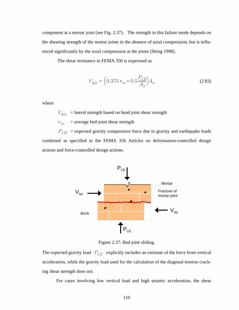
110

component at a mortar joint (see Fig. 2.37). The strength in this failure mode depends on

the shearing strength of the mortar joints in the absence of axial compression, but is influ-

enced significantly by the axial compression at the joints (Shing 1998).

The shear resistance in FEMA 356 is expressed as

(2.83)

where

= lateral strength based on bead joint shear strength

= average bed-joint shear strength

= expected gravity compressive force due to gravity and earthquake loads

combined as specified in the FEMA 356 Articles on deformation-controlled design

actions and force-controlled design actions.

Figure 2.37: Bed joint sliding.

The expected gravity load explicitly includes an estimate of the force from vertical

acceleration, while the gravity load used for the calculation of the diagonal tension crack-

ing shear strength does not.

For cases involving low vertical load and high seismic acceleration, the shear

Vbjs 0.375vte 0.5PCE

An

----------+⎝ ⎠⎛ ⎞ An=

Vbjs

vte

PCE

PCE

PCE

Vbjs

Vbjs

Mortar

Brick

Fracture of mortar joint

PCE

111

resistance in EC6 is represented by the friction of masonry relative to mortar joint and

expressed as

(2.84)

where, = constant defining the contribution of compression stresses, assumed

equal to 0.75. Therefore, for small vte, the EC6 model is 50 percent stronger than the

FEMA 356 model.

URM wall tests (Shing 1998) indicate that cyclic bed-joint sliding behavior can be

represented by an elasto-plastic hysteresis rule as shown in Fig. 2.38. Due to the loss of

cohesive force, the shear resistance drops rapidly after the peak shear force is reached. The

subsequent residual shear force is provided by the friction depending on the compressive

force in the wall. The strength in Fig. 2.38 is calculated from Eqs. 2.83 and 2.84. The elas-

tic stiffness, Ke, is discussed in Section 2.3.4, and the post elastic tangent stiffness is typi-

cally chosen as a small value for purposes of numerical stability.

Figure 2.38: Bed joint sliding behavior (Shing 1998) and uniaxial bed-joint sliding hysteresis model.

Vbjs µcPCE=

µc

Peak shear (Initial crack)

Hysteresis ModelTest

Ke

KtVbjs

∆

V

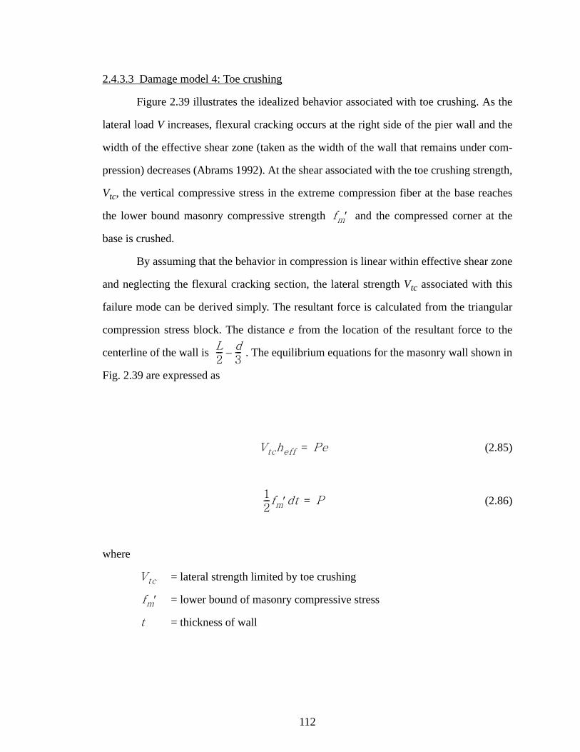
112

2.4.3.3 Damage model 4: Toe crushing

Figure 2.39 illustrates the idealized behavior associated with toe crushing. As the

lateral load V increases, flexural cracking occurs at the right side of the pier wall and the

width of the effective shear zone (taken as the width of the wall that remains under com-

pression) decreases (Abrams 1992). At the shear associated with the toe crushing strength,

Vtc, the vertical compressive stress in the extreme compression fiber at the base reaches

the lower bound masonry compressive strength and the compressed corner at the

base is crushed.

By assuming that the behavior in compression is linear within effective shear zone

and neglecting the flexural cracking section, the lateral strength Vtc associated with this

failure mode can be derived simply. The resultant force is calculated from the triangular

compression stress block. The distance e from the location of the resultant force to the

centerline of the wall is . The equilibrium equations for the masonry wall shown in

Fig. 2.39 are expressed as

(2.85)

(2.86)

where

= lateral strength limited by toe crushing

= lower bound of masonry compressive stress

= thickness of wall

fm′

L2--- d

3---–

Vtcheff Pe=

12---fm′dt P=

Vtc

fm′

t

113

Figure 2.39: Assumed effective shear zone and free body diagram of wall cracked at base.

By equating Eqs. 2.85 and 2.86, the lateral force is expressed as

(2.87)

The lower bound lateral strength in FEMA 356 is calculated as

(2.88)

Vtc

fa = P/An

heff

e L/2 - ed

L

LC

Effective Shear ZoneFlexuralCracking

P

f 'm

Vtc

P

Vtc12---P L

heff

----------⎝ ⎠⎛ ⎞ 1

4fa

3fm′-----------–⎝ ⎠

⎛ ⎞=

Vtc

Vtc αPLL

heff

---------- 1fa

0.7fm′-----------------–⎝ ⎠

⎛ ⎞=

114

where

= factor equal to 0.5 for a cantilever wall, or equal to 1.0 for fixed-fixed

pier.

= axial compressive stress calculated from 1.1 times the total gravity loads

discussed in Section 2.4.3.1

= lower bound axial compressive force 0.9 times gravity load associated

with dead load.

FEMA 356 limits the use of this equation to 0.67 < <1.00.

It should be noted that fa = P/An in the development of Eq. 2.87. However, FEMA

356 specifies two different gravity load combinations in the application of Eq. 2.88. The

axial compressive stress is calculated from the total gravity load (multiplied by 1.1)

whereas the axial compressive force is calculated only from the dead load (multi-

plied by 0.9).

The expected hysteresis behavior of this failure mode may be characterized by

moderate energy dissipation and by strength and stiffness degradation. Initiation of the

first flexural cracks may be characterized by moderate energy dissipation with negligible

strength and stiffness degradation. The post-peak response may be characterized by higher

energy dissipation but with extensive strength and stiffness degradation. The hysteresis

behavior of this failure mode may be represented by the three parameter hysteresis model

discussed previously, with pinching effects neglected.

2.4.3.4 Damage Model 5: Rocking failure

Figure 2.40 illustrates the idealized behavior associated with rocking. In a rocking

mode of failure, tension cracking occurs across a major portion of the bed joint, the com-

pression block moves toward the extreme compression fiber, and the lateral force is car-

ried by the compressed masonry. At the rocking strength Vr, an isolated wall essentially

α

fa

PL

Lheff

----------

fa

PL

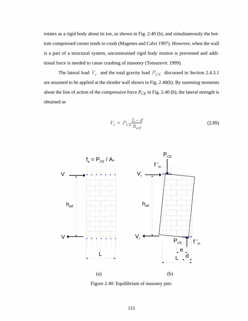
115

rotates as a rigid body about its toe, as shown in Fig. 2.40 (b), and simultaneously the bot-

tom compressed corner tends to crush (Magenes and Calvi 1997). However, when the wall

is a part of a structural system, unconstrained rigid body motion is prevented and addi-

tional force is needed to cause crushing of masonry (Tomazevic 1999).

The lateral load and the total gravity load discussed in Section 2.4.3.1

are assumed to be applied at the slender wall shown in Fig. 2.40(b). By summing moments

about the line of action of the compressive force PCE in Fig. 2.40 (b), the lateral strength is

obtained as

(2.89)

(a) (b)

Figure 2.40: Equilibrium of masonry pier.

Vr PCE

Vr PCEL d–heff

-------------=

fa = PCE / An

heff

L

V

V

PCE

heff

L

Vr

Vr

PCE

d

f 'm

f 'm

e

116

The expected rocking strength in FEMA 273 and FEMA 356 is modified from the

above equation as follows:

(2.90)

The value is the same as specified previously for the toe crushing strength calculation.

The length of compression zone d is assumed to be 0.1L (see Eq. 2.89).

In EC6, the rocking strength is calculated as

(2.91)

That is, . By equating Eq. 2.91 to the moment due to the lateral load Vr

x heff, the lateral resistance of the wall may be expressed as

(2.92)

The hysteretic energy dissipated in a typical rocking mode response is generally

small as shown in the test results (Erbay and Abrams 2002) of Fig. 2.41. There is low

energy dissipation in the tests. However, when the damage is concentrated in a bed-joint

and significant vertical loads are present, high energy dissipation is possible (Magenes and

Calvi 1997). When vertical loads are relatively low, the shaking table tests on brick

masonry walls (Magenes and Calvi 1994) show that rocking and bed joint sliding typically

take place together. The uniaxial rocking hysteresis model shown in Fig. 2.41 is used to

represent the rocking behavior. One can observe from the figure that this model assumes

zero energy dissipation. The rocking strength in Fig. 2.41 is calculated from Eqs. 2.89 and

Vr 0.9αPCEL

heff

----------=

α

PCEePCEL

2-------------- 1

fa

fm′--------–⎝ ⎠

⎛ ⎞=

eL2--- 1

fa

fm′--------–⎝ ⎠

⎛ ⎞=

Vr

PCEL

2heff

-------------- 1fa

fm′--------–⎝ ⎠

⎛ ⎞=

117

2.92. The stiffness, Ke, is taken as the wall elastic stiffness discussed Section 2.4.2, and the

post-elastic tangent stiffness shown in Fig. 2.41 is approximately zero (i.e., constant

strength). However, the test results (Magenes and Calvi 1997) show significant post-elas-

tic tangent stiffness and increasing lateral strength after the rocking strength Vr is reached.

Figure 2.41: Load history for masonry wall test (Erbay and Abrams 2002) and the assumed uniaxial rocking hysteresis model.

Figure 2.42: Example of rocking response of simple piers (Magenes and Calvi 1997).

Ke

KtVr

∆

Kt

Hysteresis ModelTest

V

Displacement (mm)

Forc

e (k

N)

118

2.4.4 Flange effects

FEMA 356 (ASCE 2000) recommends strength consideration of flange effects in

masonry walls, when the following three conditions are satisfied: 1) The face shells of hol-

low masonry units are removed and the intersection is fully grouted; 2) Solid units are laid

in running bond, and 50% of the masonry units at the intersection are interlocked; and 3)

Reinforcement from one intersecting wall continues past the intersection a distance not

less than 40 bar diameters or 24 inches. Flange effects increase the in-plane strength and

stiffness of shear walls. The influence of the orthogonal walls acting as flange elements is

generally different in tension than in compression. This influence is also a function of the

load level and any nonlinearity in the wall components. When loaded in significant ten-

sion, flexural cracking is apt to occur. In this case, the orthogonal wall may contribute sig-

nificantly to the rocking resistance, but otherwise will tend to be less effective than if it is

placed in compression. When loaded in compression, the orthogonal wall will likely pro-

vide a significant increase in the toe crushing strength. At the present time (December

2002), there is little quantitative data on flange effects in masonry walls. FEMA 356 sug-

gests that the flange effect should be considered only where the resulting flange element is

placed in compression, and that the effective flange width on each side of an in-plane wall

shall be take as the lesser of six times the thickness of the in-plane wall, half the distance

to the next wall, or the actual width of the orthogonal wall. Flange effects are modeled in

this work by assuming an in-plane wall thickness equal to the total width of the effective

flange at the location of the orthogonal wall.

2.4.5 Strength associated with a multiple story failure mode involving damage within the

lintel beams

Section 2.4.3 discusses the strength and hysteresis behavior based on pier type col-

lapse mechanisms. However, in some cases the maximum strength of a wall may be gov-

erned by a mode of failure involving substantial damage within the lintel beams along

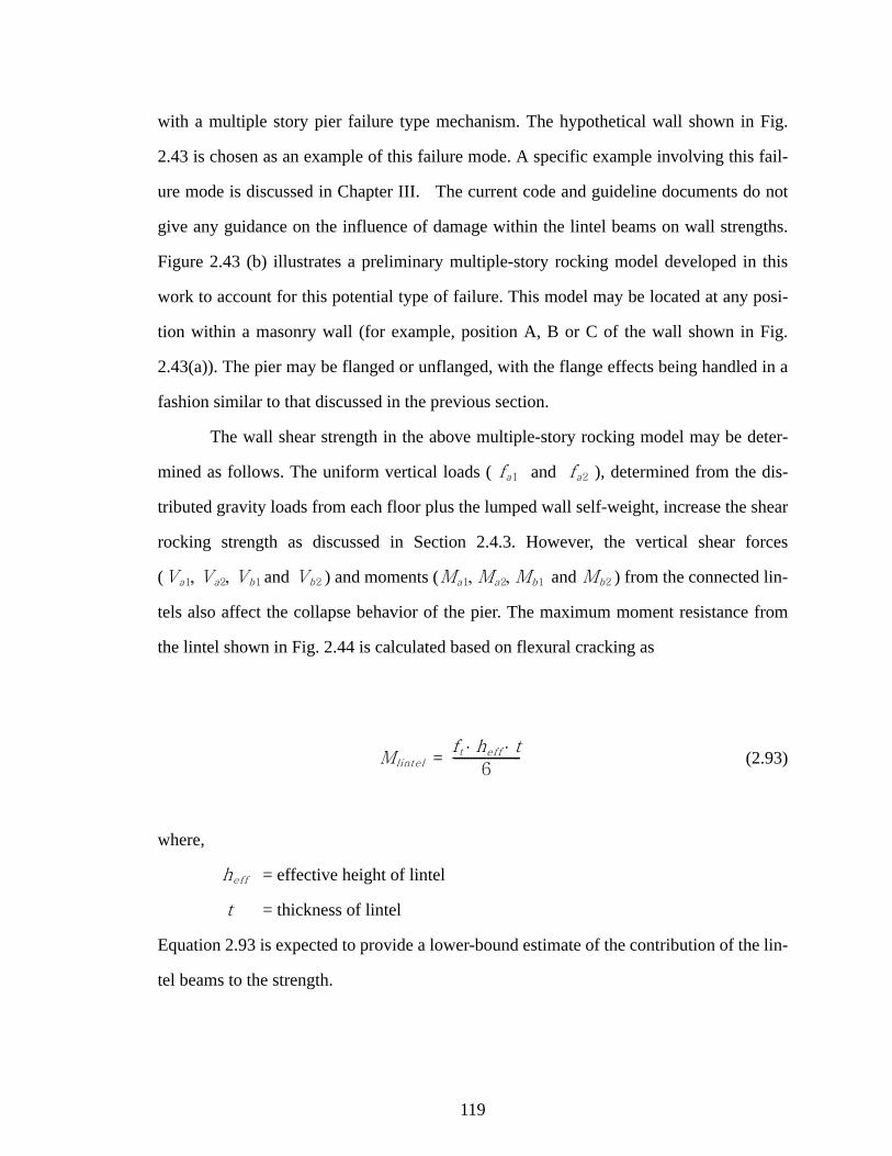
119

with a multiple story pier failure type mechanism. The hypothetical wall shown in Fig.

2.43 is chosen as an example of this failure mode. A specific example involving this fail-

ure mode is discussed in Chapter III. The current code and guideline documents do not

give any guidance on the influence of damage within the lintel beams on wall strengths.

Figure 2.43 (b) illustrates a preliminary multiple-story rocking model developed in this

work to account for this potential type of failure. This model may be located at any posi-

tion within a masonry wall (for example, position A, B or C of the wall shown in Fig.

2.43(a)). The pier may be flanged or unflanged, with the flange effects being handled in a

fashion similar to that discussed in the previous section.

The wall shear strength in the above multiple-story rocking model may be deter-

mined as follows. The uniform vertical loads ( and ), determined from the dis-

tributed gravity loads from each floor plus the lumped wall self-weight, increase the shear

rocking strength as discussed in Section 2.4.3. However, the vertical shear forces

( and ) and moments ( and ) from the connected lin-

tels also affect the collapse behavior of the pier. The maximum moment resistance from

the lintel shown in Fig. 2.44 is calculated based on flexural cracking as

(2.93)

where,

= effective height of lintel

= thickness of lintel

Equation 2.93 is expected to provide a lower-bound estimate of the contribution of the lin-

tel beams to the strength.

fa1 fa2

Va1 Va2 Vb1, , Vb2 Ma1 Ma2 Mb1, , Mb2

Mlintel

ft h⋅ eff t⋅6

-----------------------=

heff

t

120

Figure 2.43: Assumed free body diagram of a two-story pier associated with a multiple-story rocking failure.

fa1

fa2

Pce

f'm

de

L

Va1

Ma1

Va2

(1-a) Vr

a Vr

Vb2

Vb1

Mb2

Mb1

VrMr

Ma2

h 2h 1

h 1+h 2

(a) (b)

Two Story Wall

A B C

Lf

L

t

t f

Vf2

Vf1

121

Figure 2.44: Assumed stress distribution at the interface between a lintel and a pier, based on an idealized flexural cracking model.

When the flange of the pier is under compression, the rocking shear strength asso-

ciated with the above model is

(2.94)

where,

= lateral load distribution factor, 0 < a < 1 (see Fig. 2.43)

= uniform load from second floor and upper wall weight

= uniform load from roof floor and upper wall weight

= compressive uniform load from second floor and upper wall

weight at the flange area

= compressive uniform load from roof floor and upper wall weight

at the flange area

= shear force from left lintel at the second floor and roof levels

= shear force from right lintel at the second floor and roof levels

Two Story Wall

Mlintel

hlintel

Tlintel

Clintel

heff

PIER

ft

f'm

LINTEL

PIER

TensionCracking

Vr

Pcee Va Vb+( )L2---– Vf

L2--- tf

2---–⎝ ⎠

⎛ ⎞– Ma Mb+ +

h1 h2 ah2–+----------------------------------------------------------------------------------------------------------=

a

fa1

fa2

fa fa1 fa2+=

ff1

ff2

Va1 Va2,

Vb1 Vb2,

122

= area of flange

= shear force from the flange at the second floor level

= shear force from the flange at the roof level

= ultimate moment from left lintel at second floor and roof levels,

calculated from Eq. 2.93

= ultimate moment from right lintel at the second floor and roof

levels, calculated from Eq. 2.93

= lower bound of vertical compressive force

When the flange is in tension, its contribution is neglected (i.e., it is assumed that

), and thus Eq. 2.94 simplifies to

(2.95)

The calculation of Va and Vb in Eqs. 2.94 and 2.95 generally requires considerable

judgement. It is recommended that these values may be calculated by summing the down-

ward shear contribution from the lintel beams due to gravity load with the upward or

downward shear due to lateral loading. The lintel beam shears due to lateral load may be

estimated from a free-body diagram of the lintel beams, with the lintel end moments cal-

culated per Eq. 2.93.

For the two-story example illustrated in Fig. 2.43, the shear strength contributions

Va Va1 Va2+=

Vb Vb1 Vb2+=

An_flange

Vf1 ff1An_flange=

Vf2 ff2An_flange=

Vf Vf1 Vf2+=

Ma1 Ma2,

Mb1 Mb2,

Mb Mb1 Mb2+=

Ma Ma1 Ma2+=

Pce faLt Va Vb Vf+ + +=

e 0.5 LPce

fm′--------–⎝ ⎠

⎛ ⎞=

Vf 0=

Vr

Pcee Va Vb+( )L2---– Ma Mb+ +

h1 h2 ah2–+---------------------------------------------------------------------------=

123

are taken as Vr for the bottom story and (1-a) Vr for the top story.

2.4.6 Calculation of individual component stiffnesses within a parallel spring wall ideali-

zation

Each of the wall components shown in Fig. 2.28 (b) is represented by a separate

model. This analysis idealization is based on the assumption that the wall can be subdi-

vided into independent isolated components, and that these components act in parallel

within each story and in series from story-to-story. As noted at the beginning of Section

2.4, the purpose of using a separate model for each of the components is to obtain a more

quantitative representation of a perforated wall. However, the total lateral stiffness per

strength of materials models and Eq. 2.74 is typically estimated poorly as discussed in

Section 2.4.2.3. Therefore, the elastic stiffness of each wall component calculated from

the strength materials type models is modified by a single scale factor such that the total

lateral stiffness of the wall is the same as that from the plane stress analysis approach dis-

cussed in Section 2.4.2.2. The overall procedure for calculating the elastic stiffness con-

tribution from each of the components of a perforated wall is summarized in Fig. 2.45.

In the parallel spring model, the effect of the nonlinearity of each component, i.e,

the damage patterns: diagonal cracking, bed joint cracking, rocking, and toe crushing dis-

cussed in Section 2.4.3, is assumed to be localized within each component. The contribu-

tions of the other components are assumed to not be affected by the nonlinearity of a given

component.

124

Figure 2.45: The procedure of calculating the elastic stiffness contribution of the each components of a perforated wall.

2. Initial stiffness of simplified shear spring model (See Section 2.4.2.2)

Perform plane stress analysis

Find stiffness based on flexibilityapproach

1. Initial stiffness and strength of parallel spring model (See Section 2.4.2.1)

Find initial stiffness of each pier basedon strength of materials type equation

fKFEM

1=

1f

Calculate total lateral stiffness

1 2 3

∑=

=n

iiparallel kK

1

Find strength of each pier based ondamage model (See Section 2.4.3)

Calculate total lateral strength ∑=

=n

iiparallel VV

1

3. Calibration of total lateral stiffness

k1 k2 k3

Find correction factor, r, based onplane stress analysis

FEM

parallel

KK

r =

Correct initial stiffness of each pier ∑=

=n

iiicorrected krk

1_

125

2.4.7 Modeling of out-of-plane walls

FEMA 356 (ASCE 2000) suggests that the out-of-plane contributions from unre-

inforced masonry walls shall not be included in the overall modeling of the building.

However, the contributions of the out-of-plane walls to the stiffnesses and strength of rein-

forced masonry structures should be considered. The stiffness and strength contributions

from out-of-plane walls should be calculated in general based on these walls acting as iso-

lated components spanning between floor levels, and/or spanning horizontally between

the in-plane walls (ASCE 2000). The relative magnitude of these two contributions

depends on the width versus the height of the walls, the anchorages between the dia-

phragm and out-of-plane walls, and the rigidity of the flexible diaphragm. The effects of

the out-of-plane walls spanning in the horizontal direction between adjacent in-plane

walls is often small compared to the effects of the out-of-plane walls spanning in the verti-

cal direction between the diaphragms.

Figure 2.46 shows an example of out-of-plane wall modeling. The spanning of the

out-of-plane-walls between the diaphragm levels is modeled using the shear wall element

discussed previously. The deflection at the center of the flexible diaphragm in the direc-

tion of the ground motion shown in the figure is associated with the out-of-plane deforma-

tion of walls C and D. The DOFs of the out-of-plane walls are connected to the central

DOF of the diaphragm element in the proposed simplified three-dimensional model. The

out-of-plane effects from walls C and D may be modeled using a single element for conve-

nience.

The out-of-plane behavior of walls C and D is considered as uncoupled with the

in-plane behavior of these walls. That is, the influence of in-plane deformations in walls C

and D on the out-of-plane response of these walls, and the influence of the out-of-plane

bending of these walls on their in-plane response, is neglected. Also, any coupling

between the behavior of walls C and D acting as flange elements for the in-plane walls

with the above in-plane and out-of-plane behavior is not considered.

126

Figure 2.46: Three dimensional model with one diaphragm, four in-plane and one out-of-plane walls.

In the modeling of out-of-plane walls, it is assumed that the deformation of the

anchorages is negligible and that no gaps form between the out-of-plane wall and the dia-

phragm structure. If there is significant deformation of the anchorages, a appropriate

spring element can be inserted between the wall and diaphragm element to represent the

connection. The presence of deformations between the out-of-plane walls and floor/roof

diaphragms can significantly reduce the performance of the out-of-plane walls (Paquette

et al 2001).

If the out-of-plane walls are perforated, the calculation of the stiffness and strength

is difficult due to the complex behavior. The general calculation of the out-of-plane stiff-

ness and strength in these cases is not addressed directly in this research. A flexibility

based approach similar to that employed in this work for calculation of the in-plane wall

stiffnesses could be used as a potential method of determining the initial elastic out-of-

DiaphragmElement

Out-of-planewall

Wall A

Wall D

Wall B

GroundMotion

GroundMotion

GroundMotion

Wall C

: Boundary

: Node

: Direction of DOF

127

plane stiffness of these types of walls.

2.5 Summary

Details of the simplified three dimensional MDOF modeling approach proposed in

this work are presented in this Chapter. The essential analytical components of this

approach, i.e., the structural elements and procedures for calculation of the associated

stiffnesses and strengths for nonrigid diaphragms and shear walls, are discussed.

The diaphragm bending behavior of nonrigid diaphragms is assumed to be similar

to that of a horizontal plate girder. The flanges of the diaphragms resist the flexure and

the webs of the diaphragms are considered to carry the shear induced by the horizontal

forces. It is found that the bending behavior of typical diaphragms in the types of buildings

considered in this research is dominated by shear. Generally, the diaphragms also provide

coupling between the walls of the structure by acting approximately as shear panels, sub-

jected to shear raking deformations.

The proposed diaphragm element consists of six DOFs: three DOFs in the x direc-

tion and three in the y direction. An equivalent shear model is developed to provide a use-

ful and practical characterization of the diaphragm properties, and to calculate the stiffness

of the various types of horizontal wood and metal deck diaphragms in accordance with

FEMA 273 (FEMA 1997a), FEMA 356 (ASCE 2000a) and the SDI manual (SDI 1995).

The nonlinear hysteresis model specified for diaphragms accounts in general for stiffness

degradation, strength deterioration and pinching characteristics.

Two concepts for simplified wall modeling, one using a single element for each

wall and the other using multiple component elements for each wall, are discussed. A flex-

ibility based approach, based on elastic plane stress finite element analysis, is recom-

mended for accurate calculation of the initial elastic wall stiffnesses in each of these

approaches. The lateral shear strengths of in-plane walls are calculated in each of the

128

above approaches by summing the strength contributions from each of the wall compo-

nents. If a single element approach is utilized to model a complex perforated in-plane

wall, the post-elastic hysteresis response must be specified largely based on judgment. For

these cases, the wall may be modeled explicitly by separate component models connected

in parallel within each story, and connected in series from story-to-story. Strength and hys-

teresis models for unreinforced masonry walls from FEMA 356 (ASCE 2000a) and EC6

(CEN 1995) are discussed and recommendations are provided for use with the proposed

three-dimensional MDOF modeling approach. The strength and hysteresis models for the

walls are based on the limit states of pier rocking, bed-joint sliding, toe crushing and diag-

onal tension failure. Also, a preliminary model is developed that accounts for a potential

multiple-story pier rocking mode of failure involving damage within the adjacent lintel

beams.

129

CHAPTER III

SEISMIC ASSESSMENT OF A TWO-STORY LOW-RISE MASONRY BUILDING WITH FLEXIBLE DIAPHRAGMS

3.1 Introduction

This chapter addresses the seismic assessment of a two-story historic building

located in Gilroy, California, using the simplified three-dimensional analysis approach

discussed in Chapter II. This building, referred to herein as the Gilroy Firehouse, was pre-

viously studied in detail by Tena-Colunga and Abrams (1992a). In (Tena-Colunga and

Abrams 1992a), a two-dimensional discrete linear-elastic MDOF dynamic model was

developed and analyses were performed. The Gilroy Firehouse is selected for further

study in this work since its detailed as-built information is available and its strong motion

data was recorded during the Loma Prieta earthquake, which struck the San Francisco Bay

Area on October 17, 1989. Three motions at the ground floor slab and three motions at the

roof level were recorded at this building during the Loma Prieta earthquake. The building

withstood the ground shaking with little damage. Although the firehouse is located in Cal-

ifornia, its structural system is similar to typical essential buildings in Mid America.

Therefore, the study of its survival during the Loma Prieta earthquake can enhance the

understanding of essential URM buildings in Mid America.

The goals of this study are:

1. To demonstrate the use of the suggested simplified three-dimensional MDOF

approach discussed in Chapter II for a representative multiple story building

with multiple floor and roof diaphragms.

130

2. To investigate the qualities and limitations of the modeling approach discussed

in Chapter II by comparing calculated and measured results.

3. To investigate reasons why the firehouse withstood the ground shaking with lit-

tle damage.

These goals are accomplished by conducting three-dimensional linear and nonlinear anal-

yses of the Gilroy Firehouse subjected to the horizontal motions in two orthogonal direc-

tions measured at its ground floor slab. Section 3.2 describes the building, the observed

damage, and the measured motions during the earthquake. Section 3.3 explains the model-

ing of the building and the calculation of the wall and diaphragm stiffnesses and strengths

based on the best available procedures as captured within the three-dimensional analysis

approach discussed in Chapter II. Section 3.4 then presents linear analysis results based on

the above properties and compares the calculated responses to measured data.

The responses at two of the three monitored degrees of freedom are predicted rea-

sonably well by the model developed in Section 3.3. However, it is found that the correla-

tion between the calculated and measured results at one of the monitored degrees of

freedom can be improved by modifying the roof diaphragm flexural stiffness in one direc-

tion. Therefore, an additional flexural stiffness contribution is proposed in one direction

at the roof diaphragm level. Potential reasons for this increased stiffness are discussed.

Section 3.5 discusses the linear analysis results for the above modified model of the build-

ing.

Section 3.6 presents nonlinear analysis results using the wall strengths calculated

with the procedures from Chapter II. Since the physical structure sustained little damage

during the Loma Prieta earthquake, an accurate three-dimensional nonlinear analysis

model should also exhibit only minor damage. Such is the case in the model per Section

3.3 with the exception of the weakest wall of the building. Whereas minor damage was

observed in this wall within the physical structure, the model per Section 3.3 predicts sub-

stantial nonlinearity in this wall. Therefore, additional analyses are conducted to deter-

131

mine the strength required for the weakest wall such that only a modest amount of damage

is predicted.

One option that is often considered in the seismic rehabilitation of flexible dia-

phragm structures such as the Gilroy Firehouse is the stiffening and/or strengthening of

the diaphragms. Also, the diaphragm flexibility is a significant variable considered in this

research. Therefore, a useful application of the proposed three-dimensional approach is

for analysis of the sensitivity of building responses to variations in the diaphragm flexibil-

ity. Section 3.7 presents the results of sensitivity analyses in which the diaphragm stiff-

nesses of the Gilroy Firehouse are varied.

3.2 Description of the Structure

The Gilroy Firehouse, shown in Fig. 3.1, is a box-type structure with a lateral force

resisting system composed of unreinforced masonry brick walls together with flexible

wood diaphragms. The building has one interior masonry wall, as shown in Fig. 3.2. The

original structure was constructed in 1890 and survived the 1906 earthquake. The portion

of the structure to the north of the central wall was added after 1906. The central wall and

the exterior walls on the west and north side of the structure have relatively few openings

compared to the exterior walls on the south and east side of the building. Figures 3.3 and

3.4 show schematic elevations of the south and east walls. A one in. mortar joint exists

between the new portion of the east and west walls and the original structure. Three inte-

rior wood stud load bearing walls span between the second floor and roof diaphragms

north of the central wall as shown in Fig. 3.2.

Detailed plans and elevations for the firehouse are provided in Appendix B. Key

attributes of the structural system are described below.

The structure has plan dimensions of 40.1ft x 62.4 ft as shown in Fig. 3.2. The

total height of the structure is 29.17 ft as shown in Figs. 3.3 and 3.4. All the walls except

132

for the south wall are three wythe 12 in thick unreinforced brick walls. The south wall is

three wythe and is 12 in thick at the window openings, but is to 16 to 17 in thick at the

exterior piers.

The south diaphragms are almost square whereas the north diaphragms have an

aspect ratio of approximately two. The second floor diaphragms consist predominantly of

a 1/2 in. plywood overlay on 1 in. by 4 in. timbers running in the diagonal direction, nailed

to timber joists (see Fig. 3.2). A small area of the diaphragm on the northwest corner of the

second floor has 1 in tongue and groove sheathing over the diagonal timbers. The south

and north roof diaphragms have a small slope of 1:85 and 1:40, respectively. They inter-

sect the central wall at 25 in below the top of the wall, and they intersect the north and

south walls at 31 in below the top of the wall. The south roof diaphragm consists of built-

up roof trusses under 1 in.in. by 4 in. timbers running in the diagonal direction. The north

diaphragm is composed of timber sheathing running in the N-S direction. The roofing con-

sists of asphalt sheets totaling 3 in in thickness.

The diaphragms and the walls are tied with 3/4 in. diameter steel rods anchored in

the outside wythe of the walls by a hook. These ties are nominally placed every 5 ft - 1 in

at the east and west walls and every 6 ft at the south, center and north walls.

The first floor slab is 36 in thick (Tena-Colunga and Abrams 1992a). This large

thickness is a result of the ground floor being raised a number of times to match the

increasing grade elevation of the street. The building is supported on spread footings, the

dimensions and depth of which are not available. Although no specific information is

available pertaining to the type of soil, Tena-Colunga and Abrams (1992a) infer that the

site has a natural stiff soil based on inspection of the response spectra for the recorded

ground motions.

133

Figure 3.1: Firehouse at Gilroy, CA.

Figure 3.2: Second floor plan.

509 in 240 in

481

in

SouthDiaphragm

East Wall

West Wall

Nor

th W

all

Cen

tral W

all

Sou

th W

all

NorthDiaphragm

134

Figure 3.3: South wall.

Figure 3.4: East wall.

South Wall 99 in

103 in

148 in

350 in

481 in

350 in

148 in

202 in

749 in

East Wall

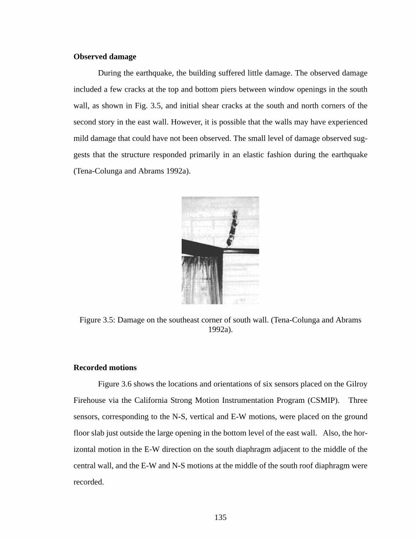
135

Observed damage

During the earthquake, the building suffered little damage. The observed damage

included a few cracks at the top and bottom piers between window openings in the south

wall, as shown in Fig. 3.5, and initial shear cracks at the south and north corners of the

second story in the east wall. However, it is possible that the walls may have experienced

mild damage that could have not been observed. The small level of damage observed sug-

gests that the structure responded primarily in an elastic fashion during the earthquake

(Tena-Colunga and Abrams 1992a).

Figure 3.5: Damage on the southeast corner of south wall. (Tena-Colunga and Abrams 1992a).

Recorded motions

Figure 3.6 shows the locations and orientations of six sensors placed on the Gilroy

Firehouse via the California Strong Motion Instrumentation Program (CSMIP). Three

sensors, corresponding to the N-S, vertical and E-W motions, were placed on the ground

floor slab just outside the large opening in the bottom level of the east wall. Also, the hor-

izontal motion in the E-W direction on the south diaphragm adjacent to the middle of the

central wall, and the E-W and N-S motions at the middle of the south roof diaphragm were

recorded.

136

The measured ground floor slab horizontal motions in the N-S and E-W directions

are shown in Figs. 3.7 and 3.8. It should be noted that the roof records were not synchro-

nized with the ground floor records (Tena-Colunga and Abrams 1992a). The roof records

are 1.78 sec out-of-phase with the ground floor records. This shift is can be observed by

comparing the motion adjacent to the central wall at the roof level (U4), shown in Fig. 3.9,

to the ground floor slab motions.

Figure 3.6: Location of sensors at the firehouse at Gilroy.

Figure 3.7: N-S direction acceleration at the ground floor slab (U1), PGA = 0.24g at 5.2 sec.

Roof Level

2nd Floor Level

Ground Level

U1

U2

U3

U6 U5

U4

N

E

-0.3

-0.2

-0.1

0.0

0.1

0.2

0.3

0 5 10 15 20

Time (sec)

Acc

eler

atio

n (g

)

137

Figure 3.8: E-W direction acceleration at the ground floor slab (U3), PGA = 0.29g at 4.48 sec.

Figure 3.9: E-W direction acceleration adjacent to the central wall (U4).

3.3 Base model (Simplified three dimensional analysis)

This section describes the application of the proposed simplified three-dimen-

sional modeling approach of Chapter II to the Gilroy Firehouse. Section 3.3.1 discusses

details of the flexible diaphragm models for this building. Section 3.3.2 presents the calcu-

lation of the stiffness and strength of the in-plane walls. Section 3.3.3 discusses the calcu-

lation of the mass properties. Section 3.3.4 explains the damping assumptions used for this

example.

Figure 3.10 shows an overall simplified three-dimensional MDOF model of the

-0.3

-0.2

-0.1

0.0

0.1

0.2

0.3

0 5 10 15 20

Time (sec)

Acc

eler

atio

n (g

)

-0.5-0.4-0.3-0.2-0.10.00.10.20.30.40.5

0 5 10 15 20

Time (sec)

Acc

eler

atio

n (g

)

138

building. Each story is modeled in a fashion similar to that shown in Fig. 1.2 except that

building has two stories.

Figure 3.10: Three-dimensional analysis model of Gilroy firehouse.

The diaphragm elements 301 and 303 represent the south diaphragms at the second

floor and roof, respectively. Diaphragm elements 302 and 304 represent the north dia-

phragms at the second floor and roof, respectively. As discussed in Section 1.4.3, each of

the nodes in this model have only one degree of freedom. The wall degrees of freedom are

associated with in-plane wall displacements. Separate nodes, each with one degree of free-

dom capture the diaphragm displacements associated with out-of-plane motion of the

walls.

11

12

1314

15

16

17

18

1

3

6

57

21

22

2324

25

26

27

28

104

101

105

102

103 Diaphragm Element ID

204

201

205

202

203

301

302

Wall Element ID

Node Number ID

303

304

629509240.5481

319

148

254.5

749

139

3.3.1 Diaphragm modeling

Section 3.3.1.1 presents the diaphragm stiffness values obtained using the FEMA

273 and 356 procedures detailed in Section 2.3.5. The diaphragm stiffnesses estimated by

Tena-Colunga and Abrams (1992a) are compared to these stiffnesses in Section 3.3.1.2.

Section 3.3.1.3 draws conclusions regarding the above stiffnesses and explains the ratio-

nale for the diaphragm stiffness values used in this research.

3.3.1.1 Equivalent shear stiffness calculation based on FEMA 273 and 356

Section 2.3.5.4 explains how to calculate the equivalent shear modulus (stiffness)

of flexible diaphragms for the proposed 3D modeling approach. Table 2.2 summarizes the

shear stiffness values (Gd) specified for various diaphragm configurations in FEMA 273

and 356. Based on the assumption that the diaphragm responses are dominated by shear-

ing type deformations, the equivalent shear moduli for the proposed modeling approach

(Ge) may be calculated from the FEMA273 and 356 stiffnesses using Eqs. 2.61 and 2.62.

Given a computed Ge value, the diaphragm bending deflection for specified lateral load-

ing in one direction is obtained using Eqs. 2.54. Therefore, Ge can be used as a common

measure of the diaphragm stiffnesses predicted by the different approaches.

Table 3.1 lists the characteristics of the different diaphragms within the Gilroy

Firehouse, and gives the corresponding Gd values from FEMA 273 and 356 as well as the

resulting Get values based on Eqs. 2.61 and 2.62. The joists within the second floor of the

building are generally supported on a ledger beam on two sides of the diaphragm, and are

anchored within wall pockets on the other two sides. Detailed information regarding

blocking within the diaphragms is not available. Four different values from FEMA 273

and 356 are reported for these diaphragms, depending on the interpretation of whether

they are blocked and/or chorded.

140

Table 3.1: Equivalent shear modulus, Ge, calculation using FEMA 273 and FEMA 356.

Diaphragm Diaphragm categorization

FEMA 273 FEMA 356

(kips/in)

Get (kips/in) (kips/in)

Get (kips/in)EW NS

2nd floor south diaphragm

(1/2” Plywood over 1” Diag.

Sheathing)

Blocked, chorded 1,800 380 533 18 9

Unblocked, chorded 900 190 267 9 5

Blocked, unchorded 700 148 207 7 4

Unblocked, unchorded 500 105 148 5 3

Roof south dia-phragm

(Built-up Roof-ing Over 1xDiag.

Sheathing)

Single diago-nal sheathing,

chorded500 105 148 5 3

2nd floor north diaphragm

(1/2” Plywood over 1” Diag.

Sheathing)

Blocked, chorded 1,800 3,623 56 18 9

Unblocked, chorded 900 1,811 28 9 5

Blocked, unchorded 700 1,409 22 7 4

Unblocked, unchorded 500 1006 16 5 3

Roof north dia-phragm

(1 x Straight Sheathing)

Straight sheathed dia-

phragm with or without chords

200 403 6 2 1

Gd_FEMA273 Gd_FEMA356

141

One can observe that the comparable diaphragm stiffnesses from FEMA 273 and

356, expressed here as the equivalent shear moduli times the equivalent thickness of the

diaphragm Get, are dramatically different from one another. This should not come as a sig-

nificant surprise, since Section 2.3.5.2 has already discussed a number of problems associ-

ated with the FEMA 273 approach. The FEMA 356 characterization of the diaphragm

stiffness is more representative of the physical response for diaphragms with relatively

small aspect ratios (e.g., L/b < 3) since it is based essentially on an idealized beam that is

rigid in flexure and flexible only in shear. Based on the FEMA 356 model, equal values

are obtained for Get in both the E-W and N-S directions. However, the FEMA 273 char-

acterization, which is based essentially on Euler-Bernoulli beam theory, predicts that Get

would differ significantly in the two orthogonal directions for the North diaphragms.

3.3.1.2 Equivalent shear stiffness calculation based on (Tena-Colunga and Abrams 1992a)

In (Tena-Colunga and Abrams 1992), the flexible diaphragms were represented by

elastic shear springs (Ks) as shown in Fig. 2.1(b). The stiffnesses (Ks) of the shear springs

for the second floor diaphragms were determined using the APA plywood diaphragm

equation (Tissell and Elliott 1997) shown in Eq. 2.48, which is based on the assumption

that the diaphragm is blocked and chorded. The Young’s modulus of the chord was taken

as 1,700ksi (Tena-Colunga and Abrams 1992a) and the shear modulus was assumed to be

60 ksi (Tena-Colunga 1998). The detailed contributions to the flexibility and stiffness

from the chord, chord splice, and nail slip were not stated by Tena-Colunga and Abrams

(1992a). Specifics of the original calculations for the straight-sheathed and diagonally-

sheathed roof diaphragms are also not available. However, it should be noted that the stiff-

ness values selected for the north roof diaphragm are identical to those for the north sec-

ond-floor diaphragm. The south roof diaphragm stiffness values are 0.87 to 0.88 of the

south second-floor diaphragm values. Table 3.2 summarizes the diaphragm stiffnesses Kd

142

from Tena-Colunga and Abrams (1992a) along with the corresponding Get values associ-

ated with the proposed 3D modeling approach.

The diaphragm stiffness (Kd) in Table 3.2 is calculated based on the fact that the

elastic shear springs shown in Fig. 2.1(b) act in parallel (i.e., Kd = 2Ks). Based on Eq.

2.15, the equivalent shear stiffness can be expressed in terms of Tena-Colunga and

Abrams’s Kd values as

and (3.1)

for the N-S and E-W directions, respectively, where:

b = 509 in /2 for south diaphragm and 240 in / 2 for north diaphragm (See Fig. 2.3)

h = 481 in /2 (See Fig. 2.3)

Table 3.2: Summary of shear spring stiffness (Kd) and equivalent shear stiffness (Get) for the discrete model of the Gilroy firehouse (Tena-Colunga and Abrams, 1992a).

Modeling Direction Diaphragm

Stiffness, Kd (kips/in)

Get (kips/in)

E-W

2nd floor south diaphragm 72.82 19

2nd floor north diaphragm 117.28 15

Roof south diaphragm 63.66 17

Roof north diaphragm 117.28 15

N-S

2nd floor south diaphragm 77.06 18

2nd floor north diaphragm 58.52 29

Roof south diaphragm 67.80 16

Roof north diaphragm 58.52 29

GethKd4b

-----------= GetbKd4h

-----------=

143

3.3.1.3 Discussion of diaphragm stiffnesses

The suggested values in FEMA 273 are not applicable as discussed in Section

3.3.1.1. The diaphragm stiffnesses suggested in FEMA 356 are smaller than the values

estimated by Tena-Colunga and Abrams (1992a). For example, the FEMA 356 Get values

for the 2nd floor south diaphragm (ranging from 3 to 9 kips/in) are smaller than the equiv-

alent shear stiffness (19 kips/in) from (Tena-Colunga and Abrams 1992a) (see Tables 3.1

and 3.2). Based on the analysis results reported subsequently in this chapter, it is apparent

that diaphragm stiffness values similar to those selected by Tena-Colunga and Abrams are

required to obtain accurate predictions of the measured building response. For this reason,

the equivalent stiffnesses shown in the fourth column (N-S direction) of Table 3.2 are cho-

sen as the diaphragm properties of the base simplified MDOF model.

The reader should note that the Get values based on (Tena-Colunga and Abrams

1992a) are similar in the E-W and N-S directions for the south second floor and roof dia-

phragms. This is expected since these diaphragms are nearly square. However, Get = 15

and 29 kips/in are obtained in the E-W and N-S directions respectively for both of the

north diaphragms. For an analysis idealization in which the diaphragm response is

assumed to be dominated by shearing deformations, it can be argued that a single value is

appropriate for Get for plywood diaphragms, straight sheathing diaphragms and the com-

bination of the two based on the fundamental mechanics of the diaphragm shearing behav-

ior (ATC 1981). For diagonally-sheathed diaphragms, the fundamental mechanics of the

diaphragm response are more complex (ATC 1981), but it is apparent that beam shear

models with equal values for Get for the two orthogonal bending directions gives a reason-

able coarse representation of the diaphragm bending stiffnesses. The FEMA 356 equa-

tions for these diaphragm types matches with this assumption about the behavior. The

larger of the two Get values determined from Tena-Colunga and Abrams’s stiffnesses is

used for the base model of the Gilroy firehouse in this work.

144

3.3.2 Wall modeling

All the in-plane walls of the Gilroy firehouse are perforated unreinforced masonry

shear walls. The flexibility approach discussed in Section 2.4.2 is used to determine the in-

plane stiffnesses of the perforated shear walls. Section 3.3.2.1 discusses the results of the

plane stress analysis of the in-plane masonry walls to obtain the flexibility coefficients.

Section 3.3.2.2 explains the in-plane wall stiffnesses calculated from the flexibility coeffi-

cients. Section 3.3.2.3 discusses the strength of the in-plane masonry walls based on the

damage models discussed in Sections 2.4.3 and 2.4.5.

3.3.2.1 Plane stress analysis of walls

Two–dimensional isoparametric plane stress finite element analyses are used to

determine flexibility coefficients for the in-plane masonry walls. The ABAQUS (HKS

1998) eight-node biquadratic plane-stress element is used for the two-dimensional finite

element wall models. The elastic modulus of the wall is taken as 515ksi. The Poison's ratio

for the analysis is 0.25. The deformed shapes and minimum principal stress contours (i.e.,

maximum compressive principal stress or minimum tensile principal stress) from these

analyses for a unit load at the roof diaphragm level are shown in Figs. 3.11 to 3.15.

A unit load is applied to each diaphragm level and the corresponding displace-

ments at the second-floor and roof levels are determined as discussed in Section 2.4.2.

These computed displacements are summarized in Tables 3.3 and 3.4. The south and north

portions of the east and west walls are modeled separately to account for the mortar joint

between these parts (see Section 3.2), based on the assumption that the lateral deflections

in each of these parts are equal but otherwise the walls are unconnected.

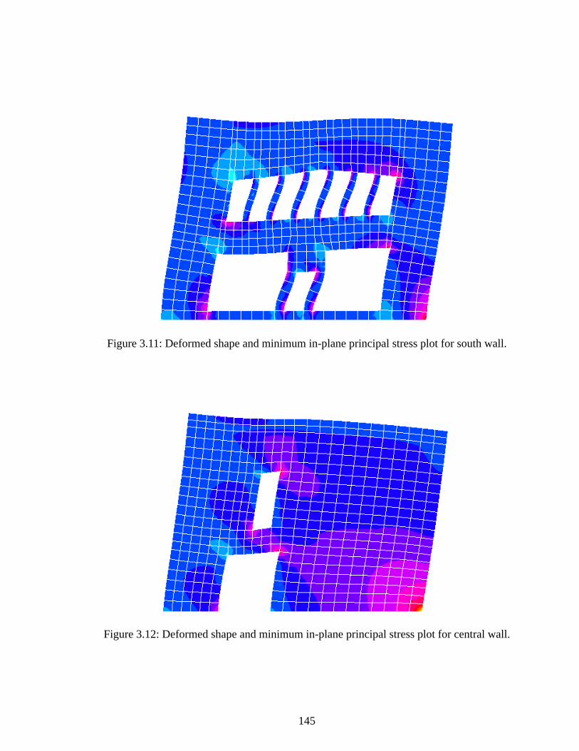
145

Figure 3.11: Deformed shape and minimum in-plane principal stress plot for south wall.

Figure 3.12: Deformed shape and minimum in-plane principal stress plot for central wall.

146

Figure 3.13: Deformed shape and minimum in-plane principal stress plot for north wall.

Figure 3.14: Deformed shape and minimum principal stress plot for east wall.

147

Figure 3.15: Deformed shape and minimum principal stress plot for west wall.

Table 3.3: Summary of displacements from plane stress analysis of the walls loaded in the E-W direction.

Wall Name Applied Load Case DOFs shown in Fig. 2.31

Displacement(Unit: in.)

South

2nd floorU1 7.216 x 10-4

U2 9.929 x 10-4

roofU1 9.929 x 10-4

U2 2.198 x 10-3

Central

2nd floorU1 2.277 x 10-4

U2 2.807 x 10-4

roofU1 2.807 x 10-4

U2 6.757 x 10-4

North

2nd floorU1 1.566 x 10-4

U2 2.013 x 10-4

roofU1 2.013 x 10-4

U2 8.511 x 10-4

148

Table 3.4: Summary of displacements from plane stress analysis of the walls loaded in the N-S direction.

3.3.2.2 Stiffness of walls

The stiffness matrices of the walls are calculated from the flexibility coefficients

shown in Tables 3.3 and 3.4 using Eqs. 2.75 through 2.79. In order to consider the mortar

joint for the east and west wall, the stiffness of south and north part of east/west wall are

Wall Applied Load Case DOFs shown in Fig. 2.31

Displacement(Unit: in.)

East South

2nd floorU1 3.169 x 10-4

U2 3.843 x 10-4

roofU1 3.843 x 10-4

U2 1.322 x 10-3

East North

2nd floorU1 3.574 x 10-3

U2 4.281 x 10-3

roofU1 4.281 x 10-3

U2 7.985 x 10-3

West South

2nd floorU1 1.454 x 10-4

U2 1.755 x 10-4

roofU1 1.755 x 10-4

U2 4.495 x 10-4

West North

2nd floorU1 7.584 x 10-4

U2 1.201 x 10-3

roofU1 1.201 x 10-3

U2 3.557 x 10-3

149

calculated separately as discussed in the previous section. The total stiffnesses of east and

west wall stiffnesses are summed from the south and north part of the walls. The final

shear stiffness of each wall is shown in Table 3.5.

Table 3.5: Wall stiffness.

3.3.2.3 Wall strength calculations

Two types of failure mechanisms, the pier type mechanism discussed in Section

2.4.3 and the multiple-story mechanism (involving damage within the lintel beams) dis-

cussed in Section 2.4.5 are considered to determine the in-plane lateral shear strength of

the south and central walls. The other wall strengths are calculated only based on the pier

type limit states. The two types of models for the south wall are illustrated in Figs. 3.16

and 3.17. For all the wall calculations, the compressive strength is taken as 1,325 ksi. This

is the average compressive strength of prism tests for the Gilroy Firehouse (Tena-Colunga

and Abrams 1992a). This strength is much higher than the recommended values in FEMA

Wall Story Stiffness (kips/in)

South 1st 2,008

2nd 1,654

Central 1st 5,263

2nd 3,739

North 1st 7,005

2nd 2,170

East1st 3,820

2nd 1,835

West1st 9,806

2nd 6,038

150

356 shown in Table 2.10. The tensile strength is taken as a representative value of 40 psi

based: flexural prism tests and bond wrench tests conducted by Erbay and Abrams (2002).

Figure 3.16: Pier-type collapse mechanism.

Figure 3.17: Multiple story type collapse mechanism.

The piers of the south wall are labeled as shown in Figs. 3.16 and 3.17 for purposes

of discussing the above two alternative strength models. The pier discretization for the

S4S2

S7 S9 S11 S12 S10 S8

S1S3

South Wall

S5 S6

S4

S2S7 S9 S11 S12 S10 S8

S1

S3

South Wall

151

other walls are shown in Figs. B.8 through B.12 in Appendix B. The height of the piers is

taken as the height of the window and door openings in each wall. The lateral strengths of

the piers are calculated using the equations discussed in Section 2.4.3. Four different fail-

ure modes are considered: diagonal tension, bed-joint sliding, toe crushing, and rocking

for each pier strength calculation. The minimum lateral strength from these models is

taken as the strength for a given pier.

For the multiple-story type collapse mechanism shown in Fig. 3.17, the right and

left side pier strengths of the south wall are calculated by using Eqs. 2.94 and 2.95. Figure

3.18 illustrates the left side pier of the south wall with the assumed lateral load distribu-

tion. Equation 2.94 is used to calculate the strength of the pier with the flange wall in com-

pression and Eq. 2.95 is used for the pier with the flange wall in tension. The variables in

these equations are summarized in Tables 3.6 and 3.7. Since the south wall is symmetric,

the total contribution from the left and right side piers is the same for lateral deflections to

the east or west.

The total lateral shear strengths of the walls are summarized in Tables 3.8 through

3.12. These strengths are obtained as the sum of the pier shear strengths.

All the piers of the south wall are governed by the rocking strength. The strength

of piers S1 and S2 of the south wall, 33.08 kips, is calculated from Eq. 2.90 (rocking

strength) based on the pier type collapse mechanism. The rocking strength of these piers

based on the multiple-story type collapse mechanism is 15.34 kips using Eq. 2.94 (for the

case of the flange wall in compression) and 15.64 kips using Eq. 2.95 (for the case of the

flange wall in tension). The strength of the pier with the flange wall in compression is

smaller than that of the pier with the flange wall in tension because the vertical load from

flange reduces the rocking strength. The minimum strength calculated for the two collapse

mechanisms is reported as shear wall strength in Table 3.8. All the piers of the other walls

are governed by rocking except pier (C2) of the central wall. This pier exhibits a bed joint

sliding behavior as indicated in Table 3.9.

152

Figure 3.18: Right side pier of the south wall.

South Wall

Vbase

2/3 Vbase

1/3 Vbase

V2lintel

V1lintel

M2lintel

M1lintel

RbaseMbase

fa2

fa1

153

Table 3.6: Variables for the pier strength in Fig. 3.17 when the flange wall is in compression.

Variable Value Variable Value

0.009 ksi 12 in

0.017 ksi 0.04 ksi

0.026 ksi

58 in for Ma1

103 in for Ma2

0.014 ksi 269.12 kips*in

0.014 ksi 848.72 kips*in

11.34 kips 1,118 kips*in

6.085 kips 78.35 kips

17.43 kips 41.33 in

72 in L 84 in

456 in2 12 in

11.7 kips 132 in

12.12 kips 202 in

23.82 kips a 1/3

fa1 t

fa2 ft

fa fa1 fa2+= heff

ff1 Ma1ft h⋅ eff t⋅6

-----------------------=

ff2 Ma2

Va1 Ma Ma1 Ma2+=

Va2 Pce faLt Va Vb Vf+ + +=

Va Va1 Va2+= e 0.5 LPcefm′--------–⎝ ⎠

⎛ ⎞=

Lf 6tf=

An_flange tf

Vf1 ff1An_flange= h1

Vf2 ff2An_flange= h2

Vf Vf1 Vf2+=

154

Table 3.7: Variables for the pier strength in Fig. 3.17 when the flange wall is in tension.

Variable Value Variable Value

10.425 kips 848.72 kips*in

3.198 kips 1,118 kips*in

13.62 kips 63.63 kips

Other values are as in Table 3.6 41.33 in

Va1 Mb2

Vb2 Mb Mb1 Mb2+=

Vb Vb1 Vb2+= Pce faLt Va Vb Vf+ + +=

e 0.5 LPcefm′--------–⎝ ⎠

⎛ ⎞=

155

Table 3.8: Shear strength and stiffness of south wall.

a. The strength is governed by rocking (Eq. 2.90) in all of the piersb. Calculated from the multiple story type collapse mechanism discussed in Section 2.4.5.

Wall (Wall ID) Stiffness (kips/in) Pier

Shear strength (kips)

Pier type mechanism for

end piersa

Multi-story type

mechanism for end piers

1st Story(101)

2,008

S1 33.08 15.34 b

S2 33.08 15.64 b

S3 1.84 1.84 a

S4 1.84 1.84 a

Total 69.84 34.66

2nd Story(201)

1,654

S5, S6 13.54

-

S7, S8 0.21

S9, S10 0.20

S11,S12 0.19

Total 28.28

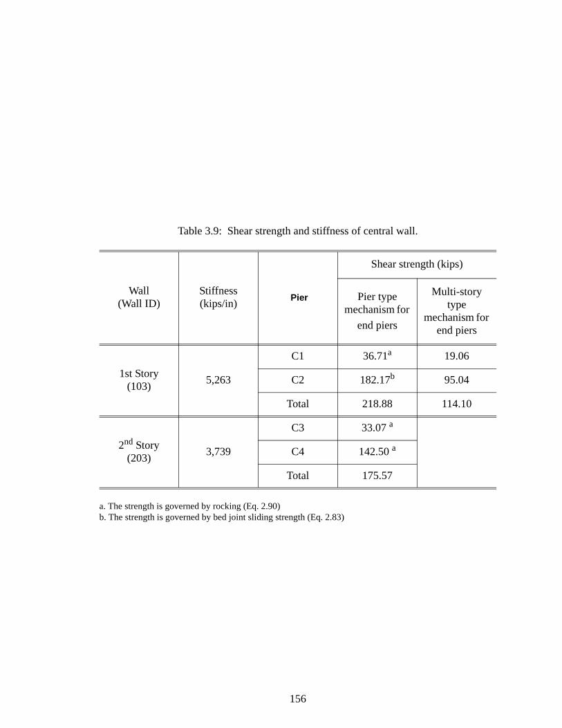
156

Table 3.9: Shear strength and stiffness of central wall.

a. The strength is governed by rocking (Eq. 2.90) b. The strength is governed by bed joint sliding strength (Eq. 2.83)

Wall(Wall ID)

Stiffness (kips/in) Pier

Shear strength (kips)

Pier type mechanism for

end piers

Multi-story type

mechanism for end piers

1st Story(103) 5,263

C1 36.71a 19.06

C2 182.17b 95.04

Total 218.88 114.10

2nd Story (203) 3,739

C3 33.07 a

C4 142.50 a

Total 175.57

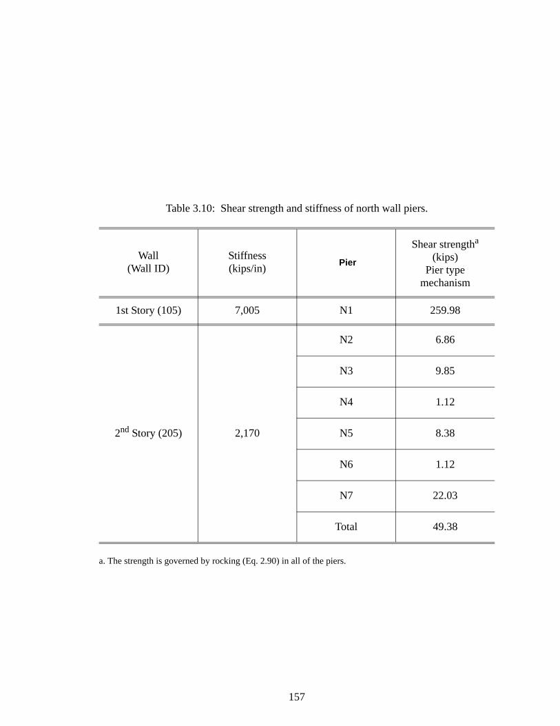
157

Table 3.10: Shear strength and stiffness of north wall piers.

a. The strength is governed by rocking (Eq. 2.90) in all of the piers.

Wall(Wall ID)

Stiffness (kips/in) Pier

Shear strengtha (kips)

Pier type mechanism

1st Story (105) 7,005 N1 259.98

2nd Story (205) 2,170

N2 6.86

N3 9.85

N4 1.12

N5 8.38

N6 1.12

N7 22.03

Total 49.38

158

Table 3.11: Shear strength and stiffness of east wall piers.

a. The strength is governed by rocking (Eq. 2.90) in all of the piers.

Wall(Wall ID)

Stiffness (kips/in) Pier

Shear strengtha (kips)

Pier type mechanism

1st Story(102) 3,820

SE1 16.59

SE2 43.49

SE3 38.15

SE4 20.77

SE5 5.43

SE6 4.43

NE1 7.97

NE2 10.97

Total 147.8

2nd Story (202) 1,835

SE7 9.75

SE8 11.25

SE9 4.26

SE10 4.75

SE11 0.89

SE12 0.74

SE13 0.68

SE14 2.05

NE3 3.70

NE4 0.74

NE5 0.92

NE6 10.84

Total 50.57

159

Table 3.12: Shear strength and stiffness of west wall.

a. The strength is governed by rocking (Eq. 2.90) in all of the piers.

3.3.3 Mass modeling

The masses of the building are obtained from the information provided by Tena-

Colunga and Abrams (199a). Table 3.13 shows the dead and live loads of the Gilroy Fire-

house. Figures 3.19 and 3.20 show the lumped mass locations at the roof and 2nd floor

level. These masses are lumped at the intersection of the centroidal axes of walls and dia-

phragms, and at the center of each diaphragm. The lumped mass distribution for the dia-

Wall (Wall ID) Stiffness (kips/in) Pier Shear strengtha (kips)

Pier type mechanism

1st Story

(104)

9,806

SW 208.45

NW1 1.90

NW2 1.33

NW3 64.04

Total 275.72

2nd Story (204) 6,038

SW 167.05

NW4 0.97

NW5 0.70

NW6 32.74

Total 201.46

160

phragms is discussed in Section 1.4.4. The gravity loads from the diaphragm are

calculated from the tributary strip areas shown in Fig. 3.19 and 3.20. The tributary masses

of the masonry walls are added to the lumped masses at the wall locations. The resulting

lumped masses used in this study are summarized in Table 3.14. The total mass of the

building is estimated as 2,745 lb-sec2/in as shown in Table 3.15.

Table 3.13: Weight consideration of the structure (Tena-Colunga and Abrams 1992a).

Figure 3.19: Lumped mass ID at 2nd floor diaphragm.

Description Weight

Self weight of the brick masonry wall 10psf /in. of thickness

Self weight of glass 8 psf

Uniform DL+LL (2nd floor level) 67.5 psf

Uniform DL+LL including Ceiling Load (roof level) 50 psf

North Diaphragm

1 2 3 4 5

6 7 8 9 10

11 12 13 14 15

161

Figure 3.20: Lumped mass ID at roof diaphragm.

South Diaphragm North Diaphragm

21 22 23 24 25

26 27 28 29 30

31 32 33 34 35

162

Table 3.14: Lumped mass calculations.

Direction Floor Mass ID Mass (lb-sec2/in)

E-W

2nd

1+6+11 279

2+7+12 318

3+8+13 339

4+9+14 144

5+10+15 208

Roof

21+26+31 280

22+27+32 270

23+28+33 342

24+29+34 128

25+30+35 203

Total 2,512

S-N

2nd

11+12+13+14+15 403

6+7+8+9+10 435

1+2+3+4+5 450

Roof

31+32+33+34+35 412

26+27+28+29+30 395

21+22+23+24+25 417

Total 2,512

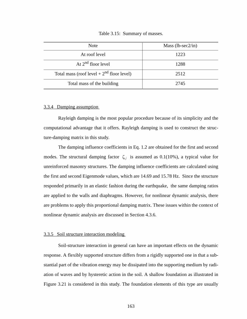
163

Table 3.15: Summary of masses.

3.3.4 Damping assumption

Rayleigh damping is the most popular procedure because of its simplicity and the

computational advantage that it offers. Rayleigh damping is used to construct the struc-

ture-damping matrix in this study.

The damping influence coefficients in Eq. 1.2 are obtained for the first and second

modes. The structural damping factor is assumed as 0.1(10%), a typical value for

unreinforced masonry structures. The damping influence coefficients are calculated using

the first and second Eigenmode values, which are 14.69 and 15.78 Hz. Since the structure

responded primarily in an elastic fashion during the earthquake, the same damping ratios

are applied to the walls and diaphragms. However, for nonlinear dynamic analysis, there

are problems to apply this proportional damping matrix. These issues within the context of

nonlinear dynamic analysis are discussed in Section 4.3.6.

3.3.5 Soil structure interaction modeling

Soil-structure interaction in general can have an important effects on the dynamic

response. A flexibly supported structure differs from a rigidly supported one in that a sub-

stantial part of the vibration energy may be dissipated into the supporting medium by radi-

ation of waves and by hysteretic action in the soil. A shallow foundation as illustrated in

Figure 3.21 is considered in this study. The foundation elements of this type are usually

Note Mass (lb-sec2/in)

At roof level 1223

At 2nd floor level 1288

Total mass (roof level + 2nd floor level) 2512

Total mass of the building 2745

ζi

164

stiff relative to the soil. Therefore, the three equivalent springs shown in this figure are

often suitable to represent the soil-structure interaction effects for simplified analysis.

In this study, the effects of soil structural interaction are neglected. The rationale

for this decision is that the soil stiffness is much larger than the stiffnesses of the in-plane

walls and diaphragms (Tena-Colunga and Abrams 1992a). Moreover, the recorded

motions were measured on the ground floor slab as shown in a SDOF model including

soil-interaction effects in Fig. 3.22. Therefore, the recorded ground motion can be applied

directly to the building without considering soil-interaction effects.

Figure 3.21: Foundation load and Uncoupled Spring Model.

Figure 3.22: SDOF model including soil-interaction effects and ground motions.

kSV ksr

ksh

P

M

H

Horizontal Spring

Rocking Spring

Mass

Wall

As(t) ; Source Ground Motion

Am(t) ; Recorded Ground Motion

165

3.4 Elastic analysis results (base model)

In this section, linear analyses are performed using the proposed MDOF model. As

discussed Section 3.2, Tena-Colunga and Abrams (1992a) also assumed that the structure

responded elastically in their analyses. The purpose of this section is to assess how the

responses of the analysis model based on the estimated properties discussed in Section 3.3

match with the measured field data. Section 3.4.1 shows the results of frequency analysis.

Section 3.4.2 compares linear time history analysis responses using the base model to

measured field data.

3.4.1 Frequency analysis

The results of frequency analysis are shown in Table 3.16. The first four mode

shapes from the Eigenvalue analysis of the building are shown in Fig. 3.23. The measured

natural periods at the roof diaphragm of the building are 0.45 and 0.33 sec. the E-W and

N-S directions, respectively. In the first mode of the building shown in Fig. 3.23, the sec-

ond floor diaphragm moves predominantly in the N-S direction, and the south roof dia-

phragm moves in the E-W direction for the second mode, the north roof diaphragm moves

in the E-W direction for the third mode, and the roof diaphragm moves in the N-S direc-

tion for the fourth mode. Therefore, in Table 3.17, the natural period of the second mode is

compared to the measured natural period in the E-W direction, and the natural period of

the fourth mode is compared to the measured natural period in the N-S direction. The rea-

son that the natural periods of this analysis are slightly higher than the ones of Tena-Col-

unga and Abrams is that the N-S directional roof diaphragm stiffnesses (see Table 3.2) are

used for this analysis. The N-S directional roof diaphragm stiffnesses are smaller than the

ones of the E-W directional stiffness. Therefore, these periods (0.417 and 0.354 sec in the

E-W and N-S directions, respectively) match well with the measured ones (0.45 and 0.33

sec in the E-W and N-S directions, respectively).

166

Table 3.16: Results of frequency analysis.

Table 3.17: Comparison of recorded vs. computed period (sec).

a. Obtained from normalized Fourier amplitude spectra (Tena-Colunga and Abrams, 1992).

Eigenmode Period (sec)

1st mode 0.428

2nd mode 0.417

3rd mode 0.359

4th mode 0.354

Location Direction Measureda Tena-Colunga and Abrams’s results

Results from this study

Roof dia-phragm

E-W 0.45 0.36 0.417

N-S 0.33 0.29 0.354

167

Figure 3.23: (a) Undeformed three-dimensional model and (b) Key mode shapes of Gilroy Fire House.

3.4.2 Time history analysis

Linear time history analysis is performed to identify the response of the structure.

The diaphragm and wall properties of the base model discussed in Sections 3.3.1 and 3.3.2

are used in this analysis. Two ground accelerations as shown in Fig. 3.7 and 3.8 are

applied at the base of the walls simultaneously in the N-S and E-W directions. For the time

history analysis, the assumed effective viscous damping is assumed as 10% based on ATC

3-06 (ATC 1978).

1st Mode 2nd Mode

3rd Mode 4th Mode

South Diaphragm North Diaphragm

South Wall

Central Wall

East Wall

Roof

2nd Floor

Ground floor

2nd floor southdiaphragm

Roof diaphragmNorth Wall

(a)

(b)

168

The computed peak responses are summarized in Table 3.18. The computed peak

displacements and accelerations in the E-W direction match well with the measured

responses at the center of the south roof diaphragm. However, the calculated peak

responses in the N-S direction at the center of south diaphragm and the responses in the E-

W direction at the top of central wall do not match well with the measured responses.

Table 3.18: Comparison of recorded vs. computed response.

a. Displacements U1 through U5 are illustrated in Fig. 3.6.

Discussion of the south roof diaphragm displacement in the N-S direction.

The calculated displacement of 0.626 in, at the center of the roof diaphragm in the

N-S direction is overestimated compared to the measured value, 0.46 in. It is expected that

the actual stiffness in the N-S direction is higher than the properties used in this analysis.

This discrepancy may be due to the influence of the trusses spanning in the N-S direction

under the roof diaphragm; combined with interior load bearing walls between central and

north walls; or out-of-plane stiffnesses of the south, central, and north walls. In order to

increase the roof diaphragm stiffness, two shear springs are added to the roof diaphragm in

Parameter MeasuredaTena-

Colunga’s results

Results from this

study

Center of south diaphragm at the roof level (E-W) U5-U3

Accel (g). 0.79 0.74 0.694

Drift (in) 1.30 1.25 1.217

Center of south diaphragm at the roof level (N-S) U6-U1

Accel (g). 0.55 0.44 0.493

Drift (in) 0.46 0.87 0.626

Top of Central Wall (E-W)U4-U3

Accel (g). 0.41 0.06 0.328

Drift (in) 0.56 0.08 0.044

169

the N-S direction (see Fig. 3.24). The estimated shear spring stiffness, Kadd, is 24 kips/in.

Figure 3.24: Added shear spring model at roof diaphragm in the N-S direction.

Discussion of central wall E-W displacements and accelerations

The measured maximum for U4 - U3 of 0.56 in. (drift of the interior wall) is much

larger than the corresponding computed value of 0.044 in. The relative displacement (U4 -

U3 = 0.56 in.) corresponds to 0.18% drift. Since this exceeds the immediate occupancy

drift ratio of 0.1% from FEMA 356, some damage would be expected. However, no dam-

age was observed within the interior wall. The above discrepancy might have resulted due

to slip between the roof diaphragm and the central wall, assuming the accelerometer was

placed on the diaphragm adjacent to the wall.

3.5 Elastic analysis results (modified base model)

The N-S directional diaphragm stiffness is modified as discussed in Section 3.4.2

and the linear analyses are repeated. Section 3.5.1 shows the results of frequency analysis.

Section 3.5.2 compares the corresponding linear time history analysis results to measured

data.

South Diaphragm North Diaphragm

N-S Direction

Kadd

: Node

Kadd

170

3.5.1 Frequency analysis

The computed periods are summarized in Table 3.19. The computed periods with

the modified stiffness are not significantly different from those shown in Table 3.16.

except for the 4th mode. which is related to the modified roof diaphragm stiffness. The

natural period of the 4th mode, 0.354 sec in Table 3.16, is decreased to 0.31 sec, due to the

shear springs. The natural periods of the Gilroy firehouse from eigenvalue analysis are

0.42 sec in the E-W direction and 0.31sec in the N-S direction, as shown in Table 3.20.

These correspond to measured natural periods of 0.45 sec in the E-W and 0.33 sec in the

N-S direction reported by Tena-Colunga and Abrams (1992a).

Table 3.19: Natural period including the diaphragm shear springs in the N-S direction.

Table 3.20: Comparison of recorded vs. computed period.

a. Obtained from normalized Fourier amplitude spectra (Tena-Colunga and Abrams, 1992a).

Eigenmode Natural Period (sec)

1st mode 0.428

2nd mode 0.417

3rd mode 0.358

4th mode 0.310

Location Direction Measureda Tena-Colunga’s results Results from this study

Roof dia-phragm

E-W 0.45 0.36 0.42

N-S 0.33 0.29 0.31

171

3.5.2 Time history analysis

The wall displacements and accelerations at the roof level are compared with mea-

sured values in Table 3.21 and Fig. 3.25 to 3.30. The computed peak displacements and

accelerations match well with the measured response. The maximum computed relative

displacements of the roof south diaphragm and the base are 1.27 and 0.46 in the E-W and

N-S directions, respectively (see Fig. 3.25). These calculated values are match well with

the measured responses (1.3 and 0.46 in. in the E-W and N-S directions, respectively). The

measured peak acceleration for the center of the south diaphragm is 0.55g compared to the

calculated one, 0.51g. The amplitude of the movement of the diaphragm (1.27 in) is high

compared to the amplitude calculated at the top of the central wall (0.05in.), as shown in

Table 3.21.

However, the measured maximum for U4 - U3 of 0.56 in (drift of the interior wall)

is still much larger than the corresponding computed value of 0.05 in. As discussed in Sec-

tion 3.4.2, the measured data at the top of the central wall may not represent the response

of the central wall. The calculated and measured displacements at the top of central wall

are compared in Fig. 3.27.

Figure 3.25: Comparison of measured and computed displacement response of roof diaphragm displacement in the E-W direction (U5-U3).

-1.5-1.0-0.50.00.51.01.5

0 5 10 15 20Time (sec)

Dis

plac

emen

t (in

) MeasuredAnalysis

172

Figure 3.26: Comparison of measured and computed displacement response of roof diaphragm displacement in the N-S direction (U6-U1).

Figure 3.27: Comparison of measured and computed displacement response of in-plane drift of interior wall at the roof level in the E-W direction (U4-U3).

Figure 3.28: Comparison of measured and computed acceleration at the top of central wall in the E-W direction (U4).

-0.6-0.4-0.20.00.20.40.6

0 5 10 15 20Time (sec)

Dis

plac

emen

t (in

) MeasuredAnalysis

-0.6-0.4-0.20.00.20.40.6

0 5 10 15 20Time (sec)

Dis

plac

emen

t (in

) MeasuredAnalysis

-0.6

-0.3

0.0

0.3

0.6

0 5 10 15 20Time (sec)

Acc

eler

atio

n(g)

Measured

Analysis

173

Figure 3.29: Comparison of measured and computed acceleration at the center of south diaphragm in the E-W direction (U5).

Figure 3.30: Comparison of measured and computed acceleration at the center of south diaphragm in the N-S direction (U6).

-0.8

-0.4

0.0

0.4

0.8

0 5 10 15 20Time (sec)

Acc

eler

atio

n(g)

Measured

Analysis

-0.6

-0.3

0.0

0.3

0.6

0 5 10 15 20Time (sec)

Acc

eler

atio

n(g)

Measured

Analysis

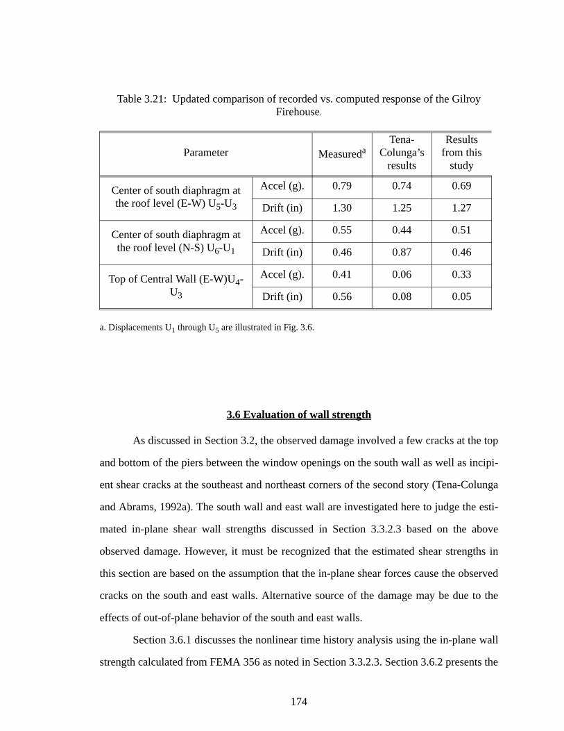
174

Table 3.21: Updated comparison of recorded vs. computed response of the Gilroy Firehouse.

a. Displacements U1 through U5 are illustrated in Fig. 3.6.

3.6 Evaluation of wall strength

As discussed in Section 3.2, the observed damage involved a few cracks at the top

and bottom of the piers between the window openings on the south wall as well as incipi-

ent shear cracks at the southeast and northeast corners of the second story (Tena-Colunga

and Abrams, 1992a). The south wall and east wall are investigated here to judge the esti-

mated in-plane shear wall strengths discussed in Section 3.3.2.3 based on the above

observed damage. However, it must be recognized that the estimated shear strengths in

this section are based on the assumption that the in-plane shear forces cause the observed

cracks on the south and east walls. Alternative source of the damage may be due to the

effects of out-of-plane behavior of the south and east walls.

Section 3.6.1 discusses the nonlinear time history analysis using the in-plane wall

strength calculated from FEMA 356 as noted in Section 3.3.2.3. Section 3.6.2 presents the

Parameter MeasuredaTena-

Colunga’s results

Results from this

study

Center of south diaphragm at the roof level (E-W) U5-U3

Accel (g). 0.79 0.74 0.69

Drift (in) 1.30 1.25 1.27

Center of south diaphragm at the roof level (N-S) U6-U1

Accel (g). 0.55 0.44 0.51

Drift (in) 0.46 0.87 0.46

Top of Central Wall (E-W)U4-U3

Accel (g). 0.41 0.06 0.33

Drift (in) 0.56 0.08 0.05

175

results of the nonlinear time history analysis using modified strengths. Section 3.6.3 dis-

cusses the out-of-plane responses associated with the diaphragm behavior.

3.6.1 Nonlinear time history analysis (base model with additional shear springs in the

N-S direction at the roof)

For the nonlinear time history analysis, the contributions from the individual com-

ponents are summed to calculate the shear strength of each masonry wall as explained in

Section 3.3.2.3. Due to the large openings in the south wall (see Fig. 3.3), its lateral shear

strength (34.66 kips) is smaller than that of the other walls (see Tables 3.8 to 3.12). When

the walls begin to damage, lateral loads tend to be redistributed to the neighboring compo-

nents along the boundaries of the flexible diaphragm. When the south wall is first dam-

aged, as shown in Fig. 3.31, lateral loads are redistributed to the east, west and central

walls due to torsional effects. The east wall on the second story and the central wall on the

first story are damaged slightly thereafter. The overall response of the building is not

changed significantly because the other walls remain elastic, as shown in Table 3.22 and

Fig. 3.31. However, there must be no damage in central wall and small displacements in

the south and east walls. It is judged that the shear strength of south wall in Table 3.8 is

underestimated based on the observed damage. The rocking strength, 34.66 kips, which is

based on the multiple story type collapse mechanism, is smaller than the 69.84 kips, which

is calculated based on the sum of the first story pier strengths. However the strengths of

south and east walls based on the pier type mechanism model are also underestimated. It is

also found that the strength of the central wall based on the multi-story mechanism is

underestimated. The nonlinear analyses are repeated to prevent significant damage on the

south and east walls and to have zero damage on the central wall by increasing the in-

plane shear strengths of these walls.

The shear strengths of the above walls necessary for the model to give results com-

parable to the observed response of the physical structure are summarized in Table 3.23.

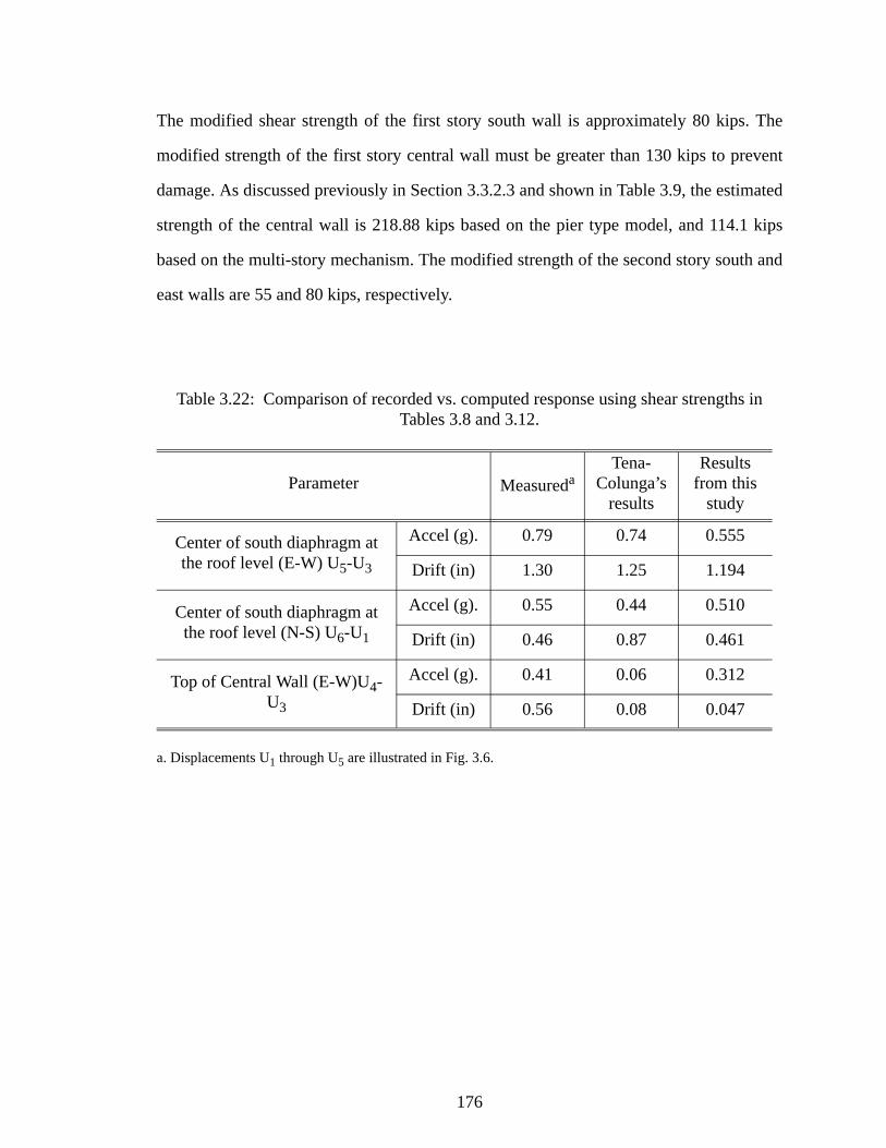
176

The modified shear strength of the first story south wall is approximately 80 kips. The

modified strength of the first story central wall must be greater than 130 kips to prevent

damage. As discussed previously in Section 3.3.2.3 and shown in Table 3.9, the estimated

strength of the central wall is 218.88 kips based on the pier type model, and 114.1 kips

based on the multi-story mechanism. The modified strength of the second story south and

east walls are 55 and 80 kips, respectively.

Table 3.22: Comparison of recorded vs. computed response using shear strengths in Tables 3.8 and 3.12.

a. Displacements U1 through U5 are illustrated in Fig. 3.6.

Parameter MeasuredaTena-

Colunga’s results

Results from this

study

Center of south diaphragm at the roof level (E-W) U5-U3

Accel (g). 0.79 0.74 0.555

Drift (in) 1.30 1.25 1.194

Center of south diaphragm at the roof level (N-S) U6-U1

Accel (g). 0.55 0.44 0.510

Drift (in) 0.46 0.87 0.461

Top of Central Wall (E-W)U4-U3

Accel (g). 0.41 0.06 0.312

Drift (in) 0.56 0.08 0.047

177

Figure 3.31: Nonlinear time history response of the building using shear strength in Tables 3.8 through 3.12.

South Wall East Wall

Roof diaphragm

-40

-20

0

20

40

-0.6 -0.3 0 0.3 0.6

Displacement (inch)

Forc

e (k

ips)

-150

-100

-50

0

50

100

150

-0.05 0 0.05

Displacement (inch)

Forc

e (k

ips)

-150

-100

-50

0

50

100

150

-0.04 -0.02 0 0.02 0.04

Displacement (inch)

Forc

e (k

ips)

Central Wall

-40-30-20-10

010203040

-0.2 -0.1 0 0.1

Displacement (inch)

Forc

e (k

ips)

South Wall

-60

-40

-20

0

20

40

60

-0.1 0 0.1

Displacement (inch)

Forc

e (k

ips)

Central Wall

-80

-60

-40

-20

0

20

40

60

-0.02 0 0.02

Displacement (inch)

Forc

e (k

ips)

East Wall

2nd Story

1st Story

178

Table 3.23: Modified shear strengths.

3.6.2 Nonlinear time history analysis (base model with modified wall strengths)

The non-linear time history analysis results are presented in this section to identify

the response of the structure using the modified shear strengths shown in Table 3.23. The

results of this analysis are not significantly different from the elastic response shown in

Table 3.21. The overall response of the building is predominantly elastic due to the slight

damage on the south and east walls, and that this damage does not significantly affect the

diaphragm responses.

Figure 3.32 shows that the south and east walls are slightly damaged and the other

walls are not damaged. It is hard to see the damage of the east wall because the strength of

the second story east wall is almost equal to the strength capacity of the wall.

Story Wall (ID) Shear strength (kips)

1st StorySouth (101) 80

Central (103) >130

2nd StorySouth (201) 55

East (202) 80

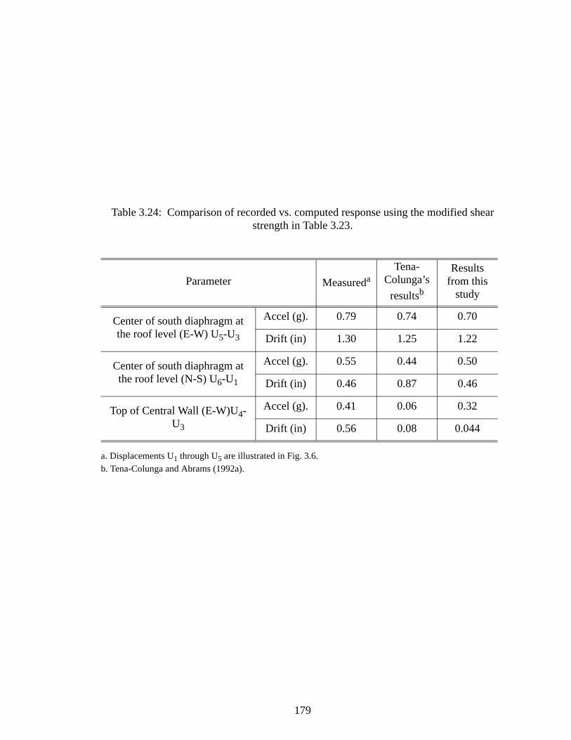
179

Table 3.24: Comparison of recorded vs. computed response using the modified shear strength in Table 3.23.

a. Displacements U1 through U5 are illustrated in Fig. 3.6.b. Tena-Colunga and Abrams (1992a).

Parameter MeasuredaTena-

Colunga’s resultsb

Results from this

study

Center of south diaphragm at the roof level (E-W) U5-U3

Accel (g). 0.79 0.74 0.70

Drift (in) 1.30 1.25 1.22

Center of south diaphragm at the roof level (N-S) U6-U1

Accel (g). 0.55 0.44 0.50

Drift (in) 0.46 0.87 0.46

Top of Central Wall (E-W)U4-U3

Accel (g). 0.41 0.06 0.32

Drift (in) 0.56 0.08 0.044

180

Figure 3.32: Nonlinear time history response of the building using updated strength shear strength.

3.6.3 Out-of-plane response

Figure 3.33 shows one example of bi-directional deformation of the diaphragms

and in-plane and out-of plane deflection of the walls taken five seconds into the time his-

tory analysis. This figure shows the significant out-of-plane movements of the diaphragm

in the E-W and N-S direction. Although out-of-plane failures are common in URM build-

South Wall East Wall

Roof diaphragm

Central Wall

South Wall Central Wall East Wall

2nd Story

1st Story

-100-80-60-40-20

020406080

100

-0.2 -0.1 0 0.1 0.2

Displacement (inch)

Forc

e (k

ips)

-150

-100

-50

0

50

100

150

-0.04 -0.02 0 0.02 0.04

Displacement (inch)

Forc

e (k

ips)

-200-150-100-50

050

100150200

-0.05 0 0.05

Displacement (inch)

Forc

e (k

ips)

-60

-40

-20

0

20

40

60

80

-0.05 0 0.05

Displacement (inch)

Forc

e (k

ips)

-80-60-40-20

020406080

-0.02 0 0.02

Displacement (inch)

Forc

e (k

ips)

-80-60-40-20

020406080

100

-0.05 0 0.05

Displacement (inch)

Forc

e (k

ips)

181

ings (ATC 1998), FEMA 356 currently does not provide any limits on out-of-plane wall

deformations for various conditions such as collapse prevention or immediate occupancy.

Such limits, or alternative checks to ensure the integrity of the walls and floors need to be

defined. Issues that need to be considered in establishing these limits include the potential

effects of bi-directional movement of walls and vertical seismic excitation of the wall ele-

ments. The peak out-of plane drift ratios of the south and east walls are 0.14% and 0.4%,

respectively, within the analysis corresponding to Fig. 3.33.

It should be noted that the out-of-plane stiffness of the URM walls is neglected in

this model as per FEMA 356 recommendations. The effects of potential contributions

from the out-of-plane wall stiffness were not studied for this building. If out-of-plane

wall stiffnesses were included, the above drifts would tend to be reduced. However, these

drifts would tend to be increased if diaphragm stiffnesses smaller than those recommended

by Tena Colunga and Abrams (1992) and closer to FEMA 356 recommended values were

used. The potential contributions from out-of-plane wall stiffness are considered within

the study presented in Chapter IV.

Figure 3.33: Displaced shape including both in-plane and out-of-plane wall deformations at 5.2 second during the time history analysis.

South Wall East Wall

2nd floor southdiaphragm

Roof diaphragm

182

3.7 Effects of diaphragm stiffness

In this section, three different diaphragms; flexible diaphragm using stiffness of

Get (see Table 3.2), diaphragm using stiffness of (3Get), and rigid diaphragm, are investi-

gated to check the responses of the building. It assumed the diaphragms remain elastic.

However, the modified strength of south and east walls and the estimated strengths of

other walls shown in Table 3.23 are used to investigate the non-linear characteristics of the

building stiffening the diaphragms. Due to stiffening of the diaphragms, the overall behav-

ior of the structure is changed. The detailed results are discussed in the following sec-

tions. Section 3.7.1 compares the calculated shear wall force and displacements. Section

3.7.2 shows the nodal responses due to the diaphragm stiffness.

3.7.1 Comparison of shear wall force and displacement

As the diaphragm stiffness, Get, in Table 3.2 are increased to 3 Get, the shear

forces of walls are not changed significantly. However, the lateral forces are distributed to

the shear walls according to the relative wall stiffnesses for the rigid diaphragm structure.

Figure 3.34 compares the responses for the flexible (Get) and rigid diaphragm structures.

As discussed in Section 3.6.2, the south and east walls of the structure with flexible dia-

phragm are damaged. However, there are no noticeable damaged walls (see Fig. 3.34) for

the structure with rigid diaphragms. When the shear force of the first story south wall

reaches to its strength capacity (80 kips), the lateral shear forces are redistributed to the

west and north walls due to the torsional effect of the rigid diaphragms. This effect

increases the north wall shear force from 62 kips to 95 kips, and the west wall shear force

from 143 kips to 191 kips. However, the shear forces of east and central walls are reduced

to 110 kip and 117 kips, respectively. From Table 3.25 and Fig. 3.35, it is found that, due

to the increased diaphragm stiffness, the lateral loads are redistributed to the stronger

walls (the north and west walls). These walls have small openings compared to the other

walls. It is also concluded that increasing the diaphragm stiffnesses three times does not

183

change significantly the lateral wall shear forces of the building compared to the rigid dia-

phragm structure. This attribute of the behavior is taken advantage of in the development

of the simplified procedures discussed in Chapter V.

Figure 3.34: Comparison of wall force and displacement between the flexible (Get) and rigid diaphragm structure.

South Wall (1st Story)

Roof diaphragm

South Wall (2nd Story)

Rigid diaphragm

Flexible diaphragm

-100-80-60-40-20

020406080

100

-0.2 -0.1 0 0.1 0.2

Displacement (inch)

Forc

e (k

ips)

-200-150-100-50

050

100150200

-0.05 0 0.05

Displacement (inch)

Forc

e (k

ips)

-60

-40

-20

0

20

40

60

80

-0.05 0 0.05

Displacement (inch)

Forc

e (k

ips)

-100-80-60-40-20

020406080

100

-0.05 0 0.05

Displacement (inch)

Forc

e (k

ips)

South Wall (1st Story)

-60

-40

-20

0

20

40

60

-0.05 0 0.05

Displacement (inch)

Forc

e (k

ips)

South Wall (2nd Story)

-150

-100

-50

0

50

100

150

-0.04 -0.02 0 0.02 0.04

Displacement (inch)

Forc

e (k

ips)

East Wall (1st Story)

East Wall (1st Story)

184

Figure 3.35: Comparison of in-plane shear forces using three different diaphragms: (a) first story and (b) second story.

0

50

100

150

South East Center West North

Shea

r for

ce (k

ips)

Get

3 Get

Rigid

050

100150200250

South East Center West North

Shea

r for

ce (k

ips)

Get

3 Get

Rigid(a)

(b)

Wall Location

Get

3Get

Rigid

Wall Location

Get

3Get

Rigid

185

Table 3.25: Comparison of peak wall displacement and shear force using three different diaphragms.

a. See Fig. 3.10.

3.7.2 Comparison of nodal responses

Increased diaphragm stiffness significantly affects the displacements and accelera-

tions at the center of the diaphragms. Fig. 3.36 and Table 3.26 compares the nodal

responses associated with stiffening of the diaphragms. The responses at the center of the

diaphragm are emphasized using bold character in the table. When the diaphragm stiff-

Wall ID

Wall Location(Element

IDa)

Flexible diaphragm model (Get) per Section

3.6.2

Flexible diaphragm

(3 Get)Rigid diaphragm

Disp.(in)

Force(kips)

Disp.(in)

Force(kips)

Disp.(in)

Force(kips)

1st Story

South (101) 0.17 80 0.16 80 0.039 80

East (102) 0.037 140 0.033 126 0.029 110

Center (103) 0.026 136 0.026 136 0.022 117

West (104) 0.015 143 0.015 143 0.013 191

North (105) 0.009 62 0.009 64 0.013 95

2nd Story

South (201) 0.043 55 0.033 55 0.029 46

East (202) 0.042 77 0.034 63 0.025 47

Center (203) 0.018 67 0.018 67 0.019 72

West (204) 0.013 76 0.012 71 0.016 97

North (205) 0.014 31 0.015 33 0.015 32

186

nesses Get are increased to 3Get, the shear wall forces are essentially unchanged, as dis-

cussed in the previous section; however, this change affects the nodal displacements and

accelerations at the center of the diaphragms significantly (see Fig. 3.36 and Table 3.26).

The displacement in the E-W direction at the center of the south roof diaphragm is

decreased from 1.221 (Get) to 0.413 in (3Get), and the displacement in the N-S direction

is decreased from 0.453 to 0.163 in. The out-of-plane displacement of the east and west

walls connected to the second floor south diaphragm is reduced from 1.22 (Get) to 0.395

in (3Get).

Figure 3.36: Comparison of displacement response using three different diaphragm stiffnesses.

0.000.010.020.030.040.05

South East Center West North

Dis

plac

emen

t (in

ch)

Get

3 Get

Rigid

0.00

0.05

0.10

0.15

0.20

South East Center West North

Dis

plac

emen

t (in

ch)

Get

3 Get

Rigid

Floor/roof diaphragmdisplacements

Get

3Get

Rigid

Get

3Get

Rigid

In-plane shear walldisplacements

1st S

tory

2nd S

tory

0.00.20.40.60.81.01.21.4

South(E-W)

North(E-W)

N-S

Dis

plac

emen

t (in

ch)

0.00.20.40.60.81.01.21.4

South(E-W)

North(E-W)

N-S

Dis

plac

emen

t (in

ch)

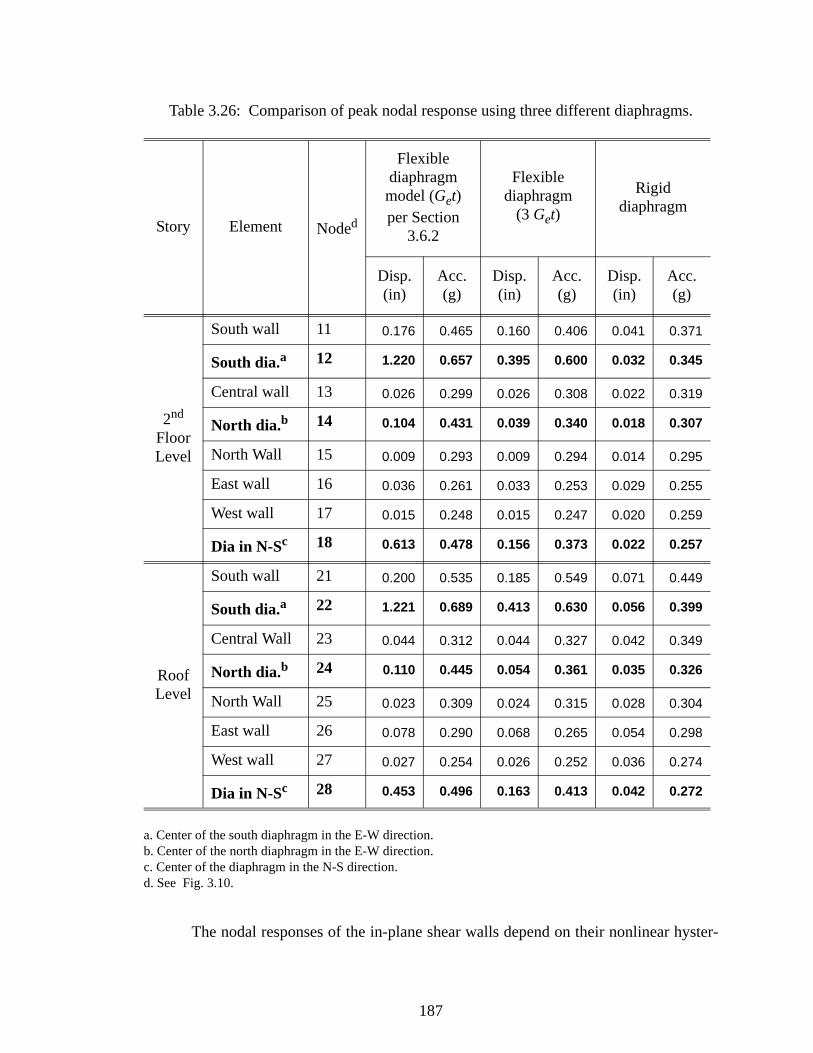
187

Table 3.26: Comparison of peak nodal response using three different diaphragms.

a. Center of the south diaphragm in the E-W direction. b. Center of the north diaphragm in the E-W direction.c. Center of the diaphragm in the N-S direction. d. See Fig. 3.10.

The nodal responses of the in-plane shear walls depend on their nonlinear hyster-

Story Element Noded

Flexible diaphragm model (Get) per Section

3.6.2

Flexible diaphragm

(3 Get)

Rigid diaphragm

Disp.(in)

Acc.(g)

Disp.(in)

Acc.(g)

Disp.(in)

Acc.(g)

2nd Floor Level

South wall 11 0.176 0.465 0.160 0.406 0.041 0.371

South dia.a 12 1.220 0.657 0.395 0.600 0.032 0.345

Central wall 13 0.026 0.299 0.026 0.308 0.022 0.319

North dia.b 14 0.104 0.431 0.039 0.340 0.018 0.307

North Wall 15 0.009 0.293 0.009 0.294 0.014 0.295

East wall 16 0.036 0.261 0.033 0.253 0.029 0.255

West wall 17 0.015 0.248 0.015 0.247 0.020 0.259

Dia in N-Sc 18 0.613 0.478 0.156 0.373 0.022 0.257

Roof Level

South wall 21 0.200 0.535 0.185 0.549 0.071 0.449

South dia.a 22 1.221 0.689 0.413 0.630 0.056 0.399

Central Wall 23 0.044 0.312 0.044 0.327 0.042 0.349

North dia.b 24 0.110 0.445 0.054 0.361 0.035 0.326

North Wall 25 0.023 0.309 0.024 0.315 0.028 0.304

East wall 26 0.078 0.290 0.068 0.265 0.054 0.298

West wall 27 0.027 0.254 0.026 0.252 0.036 0.274

Dia in N-Sc 28 0.453 0.496 0.163 0.413 0.042 0.272

188

etic behavior. For example, the displacement of the first story south wall is reduced from

0.176 (Get) to 0.041 in (3Get) for the rigid diaphragm case, because this wall is damaged

for the flexible diaphragm structures (Get and 3Get) but is not for the rigid diaphragm

structure. The nodal responses of the undamaged walls for the flexible diaphragm struc-

ture are not changed significantly. The displacement of the first story west wall is 0.015 in

for the flexible diaphragm (Get) and 0.02 in for the rigid diaphragm structure.

3.8 Summary

The Gilroy firehouse is investigated using a simple three-dimensional time history

analysis model discussed in this Chapter. The calculated responses of the building are

compared with the measured responses during the Loma Prieta Earthquake. The suggested

simplified three-dimensional MDOF model predicts well the measured response and the

observed damage with the exception of the top of the central wall. It is concluded that the

source of this disparity may have been some movement between the roof diaphragm and

the top of the central wall. Because the flexible diaphragm stiffnesses are much smaller

than those of the walls, the flexible diaphragms dominate the dynamic response of the fire-

house in both the E-W and N-S directions. Each of the four diaphragms in the building

move largely in an independent fashion.

Based on comparison to the measured responses in the physical structure, it

appears that the estimated diaphragm stiffnesses and wall strengths based on FEMA 356

are smaller than the physical values. This is consistent with the results of the diaphragm

tests conducted by Peralta et al. (2000) and discussed in Section 2.3.5.2. The sensitivity

studies conducted in this chapter indicate that the nonlinear responses of the structures

with flexible and hypothetical rigid diaphragms are significantly different. The shear wall

forces are distributed according to the relative stiffness of the walls in the hypothetical

rigid diaphragm structure. The out-of-plane displacements of the diaphragms are reduced

189

significantly when the diaphragm stiffnesses are increased three times that of the recom-

mended model for the physical structure; however, the shear wall forces are not affected

significantly. Unfortunately, appropriate drift or other limits for the out-of-plane wall

response have not been quantified at the present time (December 2002) and are not pro-

vided in FEMA 356. Therefore, it is difficult to say whether the stiffening of the dia-

phragms in the Gilroy firehouse would be appropriate or not. Obviously, the building

withstood the Loma Prieta earthquake with diaphragm displacements very similar to those

predicted by the 3D MDOF model.

190

CHAPTER IV

ANALYSIS OF A ONE-STORY LOW-RISE MASONRY BUILDING WITH A FLEXIBLE DIAPHRAGM

4.1 Introduction

Recently, two single-story single-diaphragm half-scale reinforced masonry build-

ings were tested jointly by researchers at the University of Texas at Austin and the United

States Army Construction Engineering Research Laboratory (CERL) (Cohen 2001 and

Cohen and Klingner 2001a). These experimental tests were conducted at the CERL shak-

ing table facility, and considered the seismic response under elastic conditions, moderate

damage and extensive damage. The first specimen had a diaphragm with a single layer of

diagonal-lumber sheathing. The second had a corrugated metal deck diaphragm. The first

of these tests is studied in this chapter.

The purpose of the study presented in this chapter is to assess the ability of the

general model presented in Chapter II for capture of the linear and nonlinear response of a

flexible-diaphragm building in which there are significant contributions from the out-of-

plane walls. Due to its elongated rectangular plan (L/B = 4), the seismic responses in the

E-W (short) direction were significant compared to those in N-S (long) direction. The test

results show significant nonlinear behavior of out-of-plane and in-plane walls, including

flange effects from the out-of-plane walls for shaking in the E-W direction. These and

other characteristics are not easily captured by the simple models currently provided in

code and guideline documents (Abrams 2001). Since the most significant responses in

191

the experimental tests were in the E-W direction, only the shaking in this direction is con-

sidered in this chapter.

It is difficult to determine accurately the in-plane and out-of-plane stiffness,

strength, and hysteresis using simplified equations specified in current seismic codes and

standards. In particular, it is difficult to estimate out-of-plane wall flange effects on the

response of the in-plane walls since the behavior of the out-of-plane walls is also related to

the diaphragm flexibility. Therefore, model calibration approach is adopted to predict the

structural properties. The overall geometry and topology of the building model is first

established per the concepts proposed in Chapter II. The required stiffnesses and strengths

of the components within this model are then determined by calibration to the experimen-

tal test results. The diaphragm properties are established by comparing to separate iso-

lated tests of the building diaphragm. The wall elastic stiffness properties are determined

based on one of the early shaking table tests, the strength and post-elastic stiffness proper-

ties of the out-of-plane walls are estimated based on one of the intermediate tests, and

finally the strength and post-elastic stiffness properties of the in-plane walls are computed

using the results from one of the latter CERL tests that involved significant damage to the

structure. The properties determined by this approach are compared with those calculated

from simple code and guideline type models.

After determining the model properties, sensitivity analyses are performed to

determine the influence of variations in the diaphragm flexibility, particularly the influ-

ence of the diaphragm flexibility on the in-plane and out-of-plane wall behavior.

Section 4.2 describes the test structure and summarizes the shaking table test

results. A general model based on the simplified approach from Chapter II is developed in

Section 4.3. Since the wall modeling procedures discussed in Chapter II are focused on

unreinforced masonry walls, additional studies are conducted to determine the strength

required for the reinforced masonry walls. Section 4.4 presents the model calibration pro-

cess. Sensitivity analyses are performed based on the structural properties obtained from

192

the calibration process in Section 4.5. Section 4.6 summarizes the general observations

obtained from the model calibration study and from the sensitivity analyses.

4.2 Summary of shaking table tests

The experimental test results of the building are summarized in detail by Cohen

(2001a). All experimental results in this chapter are obtained from electronic files of the

recorded test data (Cohen and Klingner 2001b and c).

4.2.1 Description of the structure

Figure 4.1 shows a schematic of the half-scale test structure. The building con-

sisted of a single wood diaphragm supported by four reinforced masonry shear walls. A

photograph of the specimen is shown in Fig. 4.2. As-built dimensions (Cohen 2001) are

shown in Figs. D.1 through D.4 of Appendix D. The height (H), length (L), and width (B)

of the building were 84, 264, and 55 in, respectively, measured from the outer-lines of

walls. The walls were composed of four-inch concrete masonry units (CMU) reinforced

vertically with #3 bars at 24 inches on center per grouted cell and reinforced horizontally

with two #3 bars at each bond beam. Bond beams were located at the tops of the openings

and in the top course of the wall. The wood diaphragm consisted of spruce-pine-fur (SPF)

3/8 in. x 3-1/4 in. diagonal lumber sheathing and SPF 3/4 in. x 5-1/2 in. roof rafters

(Cohen 2001).

4.2.2 Recorded data

Two different types of instruments -accelerometers and displacement transducers-

were used to capture the response of the building. The accelerations in the E-W direction

at the roof diaphragm were captured at five sampling locations: two locations at the top of

193

the north and south walls, and one at the center of the diaphragm, as shown in Figs. 4.3

and 4.4. The displacements in the east-west direction were captured at the top and bottom

of the west walls (see Fig. 4.4).

Figure 4.1: Overall view of test building and nodal locations for the analytical model.

Figure 4.2: Overall photograph of specimen (Cohen 2001).

Loading Direction: Sampling Location

South Wall

East Wall

North Wall

West Wall

B

H

L

Lifting Frame

Shaking Table

194

4.2.3 Overview of input base motions and observed damage

Tests 1, 3, 5, 9, and 10 of the 11 tests were in the E-W direction and corresponded

to progressively higher maximum input accelerations ranging from 0.1 to 1.33 g. Tests 2,

4 and 6 were in the N-S direction. These tests also involved progressively higher maxi-

mum input accelerations. The excitation in the E-W direction was the artificial ground

motion (C02_09s) for Carbondale, IL, developed by Wen and Wu (1999), modified to

achieve similitude (Cohen 2001). The original input time step, 0.01 sec, was reduced to

0.005 sec to maintain dynamic similitude between the half-scale structure and the full-

scale prototype (Cohen 2001). Test 5 represents the 1.0 of the C02_09s ground motion.

The excitation in the N-S direction was the artificial ground motion (C02_03s) from Wen

and Wu (1999). Test 6 corresponds to 1.0 of this ground motion. The ground motions in

all the other tests were simply scaled from those of Tests 5 and 6. Tests 7 and 8 involved

combined shaking in both the E-W and N-S directions, first with 50% of the maximum

accelerations from Tests 5 and 6 and then with 100% of these accelerations in both direc-

tions. For the analyses conducted in this dissertation, tests 3, 5, 9, and 10 are chosen from

the 11 tests results summarized by Cohen (2001).

Table 4.1 summarizes the measured peak responses, and observed damage during

Tests 3, 5, 9 and 10. Test 3 with PGA of 0.5g provides the basis for the linear elastic ana-

lytical modeling. Test 5 with PGA of 0.67g showed slight cracking in the east and west

(out-of-plane) walls. Test 9 was intended as the first test at which substantial damage to

the building would be induced. Tests 9 and 10 with PGA of 1.0g and 1.33g, respectively,

showed extensive damage of the E-W out-of-plane walls. Diagonal cracks formed at both

ends and a vertical crack formed at the center of the wall in these tests, as shown in Fig.

4.5 (Cohen 2001). When PGAs greater than 1.0g were applied to the building, significant

bed-joint cracking, characteristic of wall rocking, developed along the bottom of the north

and south in-plane walls (Cohen 2001).

Test 6, which had a PGA of 0.55g in the N-S direction exhibited some additional

195

cracking along the base of the center pier in the perforated (East) wall, and along the base

of one of the transverse (N-S) walls (Chon 2001). The data from Tests 7 and 8 is not con-

sidered within (Cohen 2001). Apparently the additional damage to the building during

these tests was small. In this chapter, the additional damage to the building within Tests 6

through 8 is assumed to be associated with the excitation in Test 9.

Figure 4.3: Photograph of diaphragm showing the location of accelerometers (Cohen 2001).

196

Figure 4.4: Instrumentation for measuring horizontal accelerations and global point displacements at roof diaphragm.

Figure 4.5: Damage to east and west walls from E-W shaking: (a) Photograph and (b) Idealized crack patterns of east and west walls (Cohen 2001).

A104b

A101a

A104a

A103aA105

A102 A106a

A103b

A106b

A101b

D104 D105 D106

D103

D101: Displacement: Acceleration

E-W direction

N-S direction

East Wall

West Wall

(a) (b)

197

Table 4.1: Summary of observed drift and damage (Cohen 2001).

4.3 Analytical modeling

The proposed simplified modeling approach discussed in Chapter II is applied to

the test building. Section 4.3.1 gives an overview of the idealized analysis model. Section

4.3.2 presents how the diaphragm model properties are obtained from a diaphragm test.

Section 4.3.3 discusses how the reinforced in-plane and out-of-plane masonry walls are

modeled. Section 4.3.4 discusses issues associated with the modeling of the input ground

motions applied to the base of the building. Section 4.3.5 describes the calculation of the

building masses. Section 4.3.6 discusses the damping model used in the analysis. Section

Test 3 5 9 10

PGA 0.50 g 0.67 g 1.00 g 1.33 g

Diaphragm Drift Ratio 0.08% 0.2% 0.35% 0.7%

out-of-plane Wall Drift Ratio (%)

0.14% (0.12 in)

0.27% (0.225in)

0.54% (0.456in)

1.1% (0.92 in)

In-Plane Wall Drift Ratio (%)

South wall

0.03% (0.026in)

0.04% (0.036 in)

0.06% (0.053 in)

0.09% (0.076 in)

North wall

0.03% (0.026in)

0.03% (0.028 in)

0.06% (0.053 in)

0.086% (0.072 in)

Damaged Elements N/A

- East and west walls (Slight cracking)

- East and west walls (Exten-sive cracking)

- South wall (bed joint cracking)

- East and west walls (Extensive cracking and hing-ing)

-South wall (bed joint cracking)

-Diaphragm (Splitting, nail pulling)

198

4.3.7 discusses other detailed issues associated with the execution of the linear and nonlin-

ear time history analysis.

4.3.1 Overview of analysis model

In order to investigate the response of the test building in the E-W direction, one

diaphragm element, four in-plane wall elements (one on each side of the diaphragm), and

one out-of-plane wall element (representing the combined effect of the East and West

walls in their out-of-plane direction) are used to model the test structure. Figure 4.6 shows

the simplified MDOF model. Each of the in-plane shear wall elements is linked to the

boundary DOFs of the diaphragm element.

Figure 4.6: Analytical model.

The out-of-plane wall element is connected to the middle DOF of the diaphragm

element, as discussed in Section 2.4.7. Section 3.2.2.1 of FEMA 356 states that for nonlin-

ear dynamic analysis, a connection between the wall and diaphragm shall be explicitly

modeled if the connection is weak and is not considered as a rigid connection (ASCE

: Boundary

: Lumped Mass

: Ground MotionDiaphragm

South Wall

North Wall

East WallWest Wall

Out-of-planewall element

199

2000). However, the diaphragm was positively anchored to all the walls and no failure of

the connections was observed in the shaking table tests (Cohen 2001). Therefore, it is

assumed that the walls are anchored to the diaphragm by rigid connections. The masses

are lumped at the corresponding degrees-of-freedom of the wall and diaphragm element.

The E-W ground motion is applied to the base of the in-plane north and south walls and to

the base of the single element model of the out-of-plane (east and west) walls (see Fig.

4.6). Detailed modeling of each of the structural components - diaphragm, in-plane walls,

and out-of-plane walls - is discussed in the next several sections.

4.3.2 Diaphragm modeling

The diaphragm element, explained in Section 2.3, consists of six degrees-of-free-

dom (DOFs): three degrees of freedom in the E-W direction and three in the N-S direction

as shown in Fig. 4.7. The diagonal lumber sheathed wood diaphragm of the test structure

is idealized as a plate girder for calculation of the diaphragm bending response as dis-

cussed in Section 2.3.1. The diaphragm element can capture three key modes: the E-W

and N-S directional bending mode; and shear raking mode. However, in the tests consid-

ered in this chapter, only the E-W bending mode is excited significantly.

Figure 4.7: Node number and the associated degree-of-freedom of diaphragm element.

u1

u2

u3

104 106

101

103

102105v1 v3v2

: Node Number

: Degree of freedom

E-W direction

N-S direction

200

The boundary walls and chord members at the tops of the east and west walls con-

nected to the diaphragm serve as the flange of the idealized plate girder. The diagonal

sheathing functions as the web. The E-W directional bending mode is significant for this

particular test building due to its long rectangular plan. The experimental tests of the dia-

phragm show that these bending displacements are dominated by shear (Cohen 2001).

Therefore, the diaphragm chord is assumed to be rigid. The web carries the shear forces

induced by the horizontal loadings. The boundary DOFs (u1, u3, v1 and v3), as shown in

Fig. 4.7, capture the in-plane wall displacements. Node 105 (v2) represents the E-W direc-

tional behavior of the diaphragm associated with the out-of-plane behavior of east and

west walls. Node 102 (u2) captures the N-S directional behavior of the diaphragm. Node

104 captures the south in-plane wall deflection and Node 106 captures the north in-plane

wall deflection.

For the diaphragm model, an equivalent shear stiffness of the diaphragm element

is obtained from the results of quasi-static diaphragm tests reported in (Cohen and Kling-

ner 2001a). A summary of these test results is presented and the estimated diaphragm stiff-

ness and strength are discussed in Section 4.3.2.1.

4.3.2.1 Summary of diaphragm test results

After the shaking table tests (see Section 4.2) were completed, the wood dia-

phragm was removed from the half-scale masonry structure (Cohen and Klingner 2001a).

The damaged components of the diaphragm (five pieces of sheathing lumber) were

removed and replaced (Cohen and Klingner 2001a). The diaphragm was supported by a

steel test frame, as shown in Fig. 4.8. It was loaded at its quarter points using two actuators

(see Figs. 4.9 and 4.10). A sequence of displacement controlled loads were applied by

monotonically, increasing the maximum displacement in what are referred to as major

cycles, each followed by several smaller-amplitude cycles, which are called minor cycles

(Cohen and Klingner 2001a). One major cycle with the following minor cycles is labeled

201

as one test number. The diaphragm was subjected to nine tests, i.e., sequences of a major

cycle followed by minor cycles.

Figure 4.8: Photograph of diaphragm test setup (Cohen and Klingner 2001a).

Figure 4.9: Plan drawing of test set up for the diaphragm (Cohen and Klingner 2001a).

202

Figure 4.10: Typical cross-section of test setup at loading points (Cohen and Klingner 2001a).

The diaphragm was displaced symmetrically in the E-W direction at its quarter points.

Figures 4.11 and 4.12 show the hysteretic relationship between the applied load and the

diaphragm drift ratio for Tests #1 - #5 and Tests #6 - #9, respectively. The diaphragm drift

ratio in these figures is defined by

(4.1)

where, . The figure for Tests

#1- #5 shows little degradation in stiffness or strength. However, Tests #6 - #9 show con-

siderable stiffness degradation and pinching effects due to the damage including nail slip-

ping, splitting of sheathing boards, and cracks in the masonry chord (Cohen and Klingner

δdiaphragm∆diaphragm0.5L

-----------------------=

∆diaphragm ∆Out of– plane– wall–∆north wall– ∆south wall–+

2--------------------------------------------------------–=

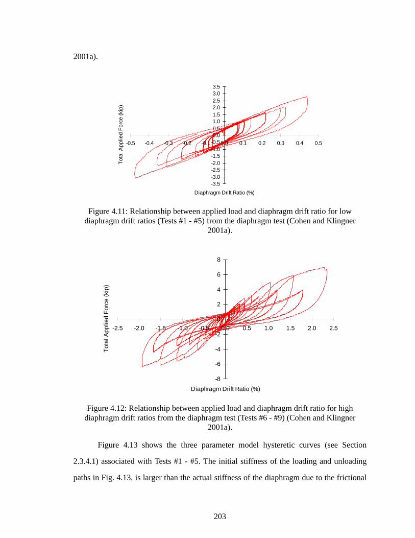
203

2001a).

Figure 4.11: Relationship between applied load and diaphragm drift ratio for low diaphragm drift ratios (Tests #1 - #5) from the diaphragm test (Cohen and Klingner

2001a).

Figure 4.12: Relationship between applied load and diaphragm drift ratio for high diaphragm drift ratios from the diaphragm test (Tests #6 - #9) (Cohen and Klingner

2001a).

Figure 4.13 shows the three parameter model hysteretic curves (see Section

2.3.4.1) associated with Tests #1 - #5. The initial stiffness of the loading and unloading

paths in Fig. 4.13, is larger than the actual stiffness of the diaphragm due to the frictional

-3.5-3.0-2.5-2.0-1.5-1.0-0.50.00.51.01.52.02.53.03.5

-0.5 -0.4 -0.3 -0.2 -0.1 0.0 0.1 0.2 0.3 0.4 0.5

Diaphragm Drift Ratio (%)

Tota

l App

lied

Forc

e (k

ip)

-8

-6

-4

-2

0

2

4

6

8

-2.5 -2.0 -1.5 -1.0 -0.5 0.0 0.5 1.0 1.5 2.0 2.5

Diaphragm Drift Ratio (%)

Tota

l App

lied

Forc

e (k

ip)

204

forces between the diaphragm and steel test frame assembly shown in Fig. 4.10 (Cohen

and Klingner 2001a). Cohen estimated that the frictional force totaled about 0.5 kips. In

this work, a frictional force of 0.4 kips is used to obtain a hysteretic curve that passes

through the origin at low levels of deflection in the linear-elastic range as shown in Figs.

4.14 and 4.15. Thus, the measured hysteretic force is separated into a frictional force and

the diaphragm force, as shown in Fig. 4.15.

Figure 4.13: Comparison of measured and analysis model for low diaphragm drift ratios (Tests #1 - #5) from the diaphragm test.

-3.5-3.0-2.5-2.0-1.5-1.0-0.50.00.51.01.52.02.53.03.5

-0.5 -0.4 -0.3 -0.2 -0.1 0.0 0.1 0.2 0.3 0.4 0.5

Diaphragm Drift Ratio (%)

Tota

l App

lied

Forc

e (k

ip)

Measured DataAnalysis Model

00

205

Figure 4.14: Frictional force for low diaphragm from the diaphragm test (Tests #1 and #2).

Figure 4.15: Contribution of friction to hysteretic curve (Cohen and Klingner 2001a).

4.3.2.2 Estimated diaphragm stiffness, strength and hysteresis model

Figures 4.16 and 4.17 compare the original experimental hysteretic curves and the

modified ones in which the frictional forces have been numerically extracted (see Fig.

4.15). The diaphragm hysteretic properties are obtained from the modified hysteretic

curves shown in these figures. The three-parameter model discussed in Section 2.3.4.1 is

implemented to characterize the diaphragm hysteresis behavior. Figures 4.18 and 4.19

compare the results of the selected three parameter hysteretic model to the modified hys-

-1.4-1.2-1.0-0.8-0.6-0.4-0.20.00.20.40.60.81.01.21.4

-0.12 -0.06 0.00 0.06 0.12

Diaphragm Drift Ratio (%)

Tota

l App

lied

Forc

e (k

ip) Frictional Force

-3

0

3

-1 0 1

F

∆

-3

0

3

-1 0 1

∆

F

-3

0

3

-1 0 1

F

∆ - =Measured

Hysteretic Curve Frictional Force ModifiedHysteretic Curve

206

teretic curves.

It must be recognized that this diaphragm was damaged during the previous shak-

ing table tests (Cohen 2001). Even if the visually damaged components of this diaphragm

were removed and replaced, the stiffness and strength of the diaphragm in the shaking

table test building may be slightly larger. Therefore, the stiffness and strength properties of

the diaphragm are increased 10% over those of the measured hysteretic properties. The

backbone curve is shown in Fig. 4.20.

Figure 4.16: Comparison of measured and modified hysteretic curve in which frictional forces are extracted from measured forces for low diaphragm drift ratios (Tests #1 - #5).

-3.5-3.0-2.5-2.0-1.5-1.0-0.50.00.51.01.52.02.53.03.5

-0.5 -0.4 -0.3 -0.2 -0.1 0.0 0.1 0.2 0.3 0.4 0.5

Diaphragm Drift Ratio (%)

Tota

l App

lied

Forc

e (k

ip)

Measured hysteretic curve

Modified hysteretic curve (=Total applied force - Frictional force)

207

Figure 4.17: Comparison of measured and modified hysteretic curve in which frictional forces are extracted from measured forces for low diaphragm drift ratios (Tests #6 - #9).

Figure 4.18: Diaphragm analysis model associated with the modified hysteretic curve for Tests #1- #5.

-8

-6

-4

-2

0

2

4

6

8

-2.5 -2.0 -1.5 -1.0 -0.5 0.0 0.5 1.0 1.5 2.0 2.5

Diaphragm Drift Ratio (%)

Tota

l App

lied

Forc

e (k

ip)

Measured hysteretic curve

Modified hysteretic curve (=Total applied force - Frictional force)

-3.5-3.0-2.5-2.0-1.5-1.0-0.50.00.51.01.52.02.53.03.5

-0.5 -0.4 -0.3 -0.2 -0.1 0.0 0.1 0.2 0.3 0.4 0.5

Diaphragm Drift Ratio (%)

Tota

l App

lied

Forc

e (k

ip)

Modified hysteretic curve (=Total force - Frictional force)

Analysis Model

208

Figure 4.19: Diaphragm analysis model associated with the modified hysteretic curve for Tests #6- #9.

Figure 4.20: Comparison of hysteresis envelopes.

-9

-7

-5

-3

-1

1

3

5

7

9

-2.5 -2.0 -1.5 -1.0 -0.5 0.0 0.5 1.0 1.5 2.0 2.5

Diaphragm Drift Ratio (%)

Tota

l App

lied

Forc

e (k

ip)

Modified hysteretic curve (=Total force - Frictional force)

Analysis Model

0123456789

0.0 0.5 1.0 1.5 2.0 2.5

Diaphragm Drift Ratio (%)

Tota

l App

lied

Forc

e (k

ip)

Modified hysteretic curve (=Total force - Frictional force)

Backbone curve comprising peak envelope of modified hysteretic curve

Backbone curve compensating the damages of the shaking table test building

209

The final selected stiffness and strength properties of the diaphragm are shown in

Fig. 4.21. The elastic stiffness of the diaphragm is 9.05 kips per one percent drift. This cal-

culated total stiffness the diaphragm is 7.41 kips/in. This stiffness value is similar to

(8 kips/in) for a chorded single diagonally sheathed diaphragm (see Table 2.2).

In Cohen’s research, the structure was idealized as a two-degrees-of-freedom sys-

tem as shown in Fig. 2.1. The first degree of freedom was associated with the in-plane

deformation of the north and south walls, and the second one is associated with the in-

plane deformation of the flexible diaphragm. The estimated diaphragm stiffness of the two

DOF model was 24 kips/in (Cohen 2001). The difference between 24 and 7.41 kips/in may

be due to the effects of the out-of-plane wall. In the two DOF model, the out-of-plane

wall stiffness was not considered. The diaphragm properties selected from the quasi-static

diaphragm tests are used in the current work.

The equivalent shear properties of the diaphragm (see Section 2.3.5.4) are calcu-

lated from the modified backbone curve shown in Fig. 4.20. The behavior of this dia-

phragm is governed by shear deformation. The equivalent width of the diaphragm is

calculated from the mid-thickness of the walls. The equivalent shear stiffness, Get, and the

equivalent shear stress is calculated from these equivalent properties and these values are

used in the analysis input discussed in Section 2.3.

The calculated effective elastic and tangent shear stiffness for the three parameter

hysteretic model are 8.82 kips/in (Get)1 and 1.95 kips/in (Get)3, respectively, as shown in

Fig. 4.21. The first (F1) and second shear stresses (F2) at the points where the stiffness

changes, as explained in Sections 2.4.3, are 0.1 ksi (0.65kips) and 0.69 ksi (4.46 kips),

respectively. The , and parameters are 3.0, 0.01, and 0.478, respectively.

4.3.3 Wall modeling

The dimensions of the north and south walls are 55 (B) x 84 (H) in, and the east

Gd_FEMA356

α β γ

210

wall and west walls are 264 (L) x 84 (H) in as shown in Figs. 4.1 and 4.22. There were

openings in the east wall. The strength of materials models discussed in Section 2.4 apply

only to unreinforced masonry shear walls. The strengths and stiffnesses of the in-plane

and out-of-plane reinforced masonry walls are estimated using the mechanics of materials

type equations from FEMA 356 (ASCE 2000a) and ACI 530-99 (MSJC 1999b) in this

Section. In order to obtain estimates of the actual properties of the test structure in this

research, a model calibration process shown in Fig. 4.34 is used.

211

Figure 4.21: Summary of hysteretic properties of three parameter model for diaphragm element: (a) Stiffness and strength, (b) Hysteresis model.

-8

-6

-4

-2

0

2

4

6

8

-2 -1 0 1 2

Diaphragm Drift Ratio (%)

Tota

l App

lied

Forc

e (k

ip)

αF2

F2

γF2

(γ=0.478)

(α = 3)

β*dE/F2

dE

(β = 0.01)

0

2

4

6

0 1Diaphragm Drift Ratio (%)

Tota

l App

lied

Forc

e (k

ip)

F1=0.65

0.07 0.67

F2=4.46

K1 = 9.05 kips/%( (Ge t)1=8.82 kips/in)

K2 = 6.37 kips/%( (Ge t)2 = 6.21 kips/in)

K3 = 2.00 kips/%( (Ge t)3= 1.95 kips/in)

(a)

(b)

212

4.3.3.1 Material properties from prism masonry compression tests versus predicted values

Compression tests were performed by CERL personnel. Measured mechanical

properties of the masonry used in the test building were provided in (Cohen 2001). Table

4.2 summarizes the experimental test of the CMU used in the test building. The masonry

compression prism tests from Cohen (2001a) showed that the grouted and ungrouted

strengths were 1.4 ksi and 0.9 ksi, respectively. The elastic moduli of the grouted and

ungrouted half-scale concrete masonry units (CMU) were 330 ksi and 320 ksi, respec-

tively (Cohen 2001). When Eq. 2.66 is used along with fm’ = 1.4 ksi from Table 4.2, a

value of Em = 770 ksi is obtained for the grouted compressive strength. It can be con-

cluded that Eqs 2.66 to 2.69 do not provide an accurate estimate of the elastic modulus of

the masonry in compression, Em, for this test. In the analyses subsequently reported in this

chapter, the average values of Em = 325 ksi and fm’ = 1.15 ksi from Table 4.2 are used for

the subsequent analyses.

Table 4.2: Masonry prism compression tests (Cohen 2001).

ConstructionCompressive strength

(fm’)Elastic modulus

(Em) Usable strain

grouted 1,400 psi 330 ksi 0.0029

ungrouted 900 psi 320 ksi 0.0029

213

Figure 4.22: Reinforcement of masonry walls: (a) North and south wall; (b) East wall; (c) Plan; (d) North and south wall detail; and (e) East and west wall detail (Cohen 2001).

(a) (b)

(c)

one #3 reinforcingbar per grouted cell

two #3 reinforcingbars per bond beam

D

(d) (e)

one #3 reinforcingbar per grouted cell

s

beff

t

t

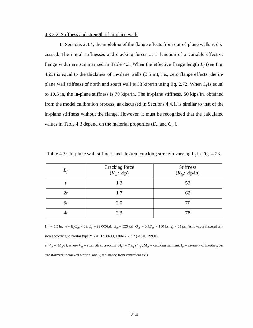
214

4.3.3.2 Stiffness and strength of in-plane walls

In Sections 2.4.4, the modeling of the flange effects from out-of-plane walls is dis-

cussed. The initial stiffnesses and cracking forces as a function of a variable effective

flange width are summarized in Table 4.3. When the effective flange length Lf (see Fig.

4.23) is equal to the thickness of in-plane walls (3.5 in), i.e., zero flange effects, the in-

plane wall stiffness of north and south wall is 53 kips/in using Eq. 2.72. When Lf is equal

to 10.5 in, the in-plane stiffness is 70 kips/in. The in-plane stiffness, 50 kips/in, obtained

from the model calibration process, as discussed in Sections 4.4.1, is similar to that of the

in-plane stiffness without the flange. However, it must be recognized that the calculated

values in Table 4.3 depend on the material properties (Em and Gm).

Table 4.3: In-plane wall stiffness and flexural cracking strength varying Lf in Fig. 4.23.

1. t = 3.5 in, n = Es/Em = 89, Es = 29,000ksi, Em = 325 ksi, Gm = 0.4Em = 130 ksi, fr = 68 psi (Allowable flexural ten-

sion according to mortar type M - ACI 530-99, Table 2.2.3.2 (MSJC 1999a).

2. Vcr = Mcr/H, where Vcr = strength at cracking, Mcr = (frIgt) / yt , Mcr = cracking moment, Igt = moment of inertia gross

transformed uncracked section, and yt = distance from centroidal axis.

LfCracking force

(Vcr: kip)Stiffness

(Kip: kip/in)

t 1.3 53

2t 1.7 62

3t 2.0 70

4t 2.3 78

215

The shear strength of the in-plane wall can be calculated from Eq. 4.2 (ASCE

2000a).

: Eq. 7-11 in FEMA 356 (4.2)

where

= Lower bound shear strength provided by masonry

= Area of net mortared / grouted section

= Moment on the masonry section

= Shear on the masonry section

= Wall length in direction of shear force

= Lower-bound vertical compressive force in pounds due to gravity loads

If , Eq. 7-11 in FEMA 356 becomes

(4.3)

is 5.2 kips using Eq. 4.3 with H = 84 in, = 53 in, and = 656 lb.

Since the shear strength is from this calculation is greater than the flexural cracking

strength from Table 4.3, it is apparent that the primary damage within the wall will be

flexural cracking.

The yield strength of the in-plane wall without flange effects from the east and

west walls is calculated from Fig. 4.23. The fraction of the structural depth of the wall in

compression is calculated as

VmL 4.0 1.75MVdv-----------⎝ ⎠⎛ ⎞– An fm′ 0.25PL+=

VmL

An

M

V

dv

PL

M VH=

VmL 4.0 1.75Hdv------⎝ ⎠⎛ ⎞– An fm′ 0.25PL+=

VmL dv PL

216

(4.4)

Where

= area of nonprestressed tension reinforcement (0.11 in2 )

= structural depth (53.13 in)

= distance between compression reinforcements in Fig. 4.23 (27.44 in)

= distance from extreme compression fiber to centroid of compression

reinforcement (1.75 in)

= effective thickness of hollow CMU (2.2 in)

The specified yield strength of the nonprestressed reinforcement is 31.92 ksi,

which is 30 percent larger than the allowable strength of 24 ksi. The calculated values of

the forces Ts1, Ts2, and Cs shown in Fig. 4.23 are 3.51, 0.87, and 1.43 kips, respectively.

The yielding moment, My, is 190 kips-in, and the shear strength, Vy, is 2.26 kips. When

the flange effect is considered, this strength value is increased depending on the magni-

tude of Lf. However, the flange effect is assumed to be zero in this work for the purpose of

obtaining a lower-bound estimate of the in-plane wall properties (flange effects from the

out-of-plane walls are considered within the calibration process).

kdcd------=

3nAs– nAs 9nAs 2d1teff– 2d3teff 4dteff+ +( )+[ ]dfm′teff

------------------------------------------------------------------------------------------------------------------------------------------- 0.312= =

As

d

d2

d3

teff

217

Figure 4.23: In-plane wall detailed section.

With flange Without flange

A-A Section

V

V M = V H

H = 84 in

A A

d3 = 1.75 in

d1 =27.44 in

d2 =23.94 in

kd = 16.58 in

Ts1

Ts2

Cs Cc

jd = 47.6 in

one #3 reinforcingbar per grouted cell

(As = 0.11 in2 )

Lf

54.87 in

3.5 in

3.5 in

54.87 in

218

4.3.3.3 Stiffness and strength of out-of-plane walls

Strength of out-of-plane walls

The strength contribution from the out-of-plane walls is calculated based on Fig.

4.24. Flexural cracking of the out-of-plane masonry wall may lead to significant damage.

The effective compression width per bar as beff in Figs. 4.22 and 4.24, is 21 in. This value

is obtained as the smallest of the center-to-center bar spacing (22 in), six times the wall

thickness (21 in), or 72 in (ACI 530-99 Section 2.3.3.3) (MSJC 1999b). The calculated

flexural cracking moment Mcr is 2.8 kips-in per effective width using the information in

the footnotes to Table 4.3. The cracking strength is 1.62 lb/in. When this strength is

applied to the total length of out-of-plane wall (427 in), the flexural cracking force Vcr is

0.691 kips.

The fraction of the structural depth of the wall in compression k = dc/d is 0.137

from Fig. 4.24. The yielding moment My is 280 lb-in per in. The yielding force per unit

length is 3.33 lb, and the total flexural yielding force, Vy , is 1.42kip.

Figure 4.24: Compressive area for out-of-plane masonry wall.

one #3 reinforcingbar per grouted cell

beff

t

Cc

Ts

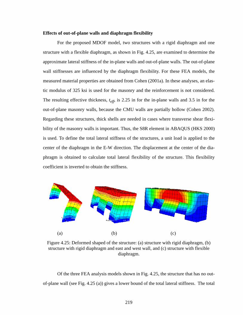
219

Effects of out-of-plane walls and diaphragm flexibility

For the proposed MDOF model, two structures with a rigid diaphragm and one

structure with a flexible diaphragm, as shown in Fig. 4.25, are examined to determine the

approximate lateral stiffness of the in-plane walls and out-of-plane walls. The out-of-plane

wall stiffnesses are influenced by the diaphragm flexibility. For these FEA models, the

measured material properties are obtained from Cohen (2001a). In these analyses, an elas-

tic modulus of 325 ksi is used for the masonry and the reinforcement is not considered.

The resulting effective thickness, teff, is 2.25 in for the in-plane walls and 3.5 in for the

out-of-plane masonry walls, because the CMU walls are partially hollow (Cohen 2002).

Regarding these structures, thick shells are needed in cases where transverse shear flexi-

bility of the masonry walls is important. Thus, the S8R element in ABAQUS (HKS 2000)

is used. To define the total lateral stiffness of the structures, a unit load is applied to the

center of the diaphragm in the E-W direction. The displacement at the center of the dia-

phragm is obtained to calculate total lateral flexibility of the structure. This flexibility

coefficient is inverted to obtain the stiffness.

(a) (b) (c)

Figure 4.25: Deformed shaped of the structure: (a) structure with rigid diaphragm, (b) structure with rigid diaphragm and east and west wall, and (c) structure with flexible

diaphragm.

Of the three FEA analysis models shown in Fig. 4.25, the structure that has no out-

of-plane wall (see Fig. 4.25 (a)) gives a lower bound of the total lateral stiffness. The total

220

lateral stiffness of north and south in-plane walls in this model is 80 kips/in. This value is

the same as that calculated from the simplified mechanics of materials types of approaches

using Eq. 2.72. The total lateral stiffness of the structure with the rigid diaphragm (see Fig.

4.25 (b)) is 257 kips/in. The lateral stiffness of the second structure is almost three times

larger than that of first structure that has no out-of-plane walls. The reason is that the

shear stiffness and axial effect in east and west out-of-plane walls contributes to the total

lateral stiffness, as shown in Fig. 4.26.

Figure 4.25 (c) shows the deformed shape of the structure with a flexible dia-

phragm. This deformed shape is more complex than the previous ones. The north and

south walls are twisted due to the bending of the flexible diaphragm. The out-of-plane

wall stiffness and strength is affected by the out-of-plane bending associated with the dia-

phragm deformation. It is difficult to determine the wall properties by simple principles in

this case.

Figure 4.26: Shear and axial force contribution of out-of-plane walls.

The stiffnesses of these structures are summarized in Table 4.4. The total lateral

stiffness of the structure with flexible diaphragm is estimated by using the model calibra-

tion process discussed in Sections 4.4. The total lateral stiffness from the model calibra-

LateralLoad

Diaphragm

East out-of-plane wall

West out-of-plane wall

Shear forceShear force

Axial force

Axial force

221

tion process is 23 kips/in including in-plane and out-of-plane wall stiffness. These

stiffnesses are discussed subsequently in Sections 4.4. It is apparent that the total lateral

stiffness is dramatically decreased due to the diaphragm flexibility. The detailed out-of-

plane wall effects are discussed in Sections 4.4 and 4.5.

Table 4.4: Comparison of stiffnesses in terms of diaphragm flexibility and out-of-plane walls without considering reinforcement.

Observed wall damage and hysteretic models

In this work, the damage sustained by the building is characterized using drift

ratios. The drift ratios of the in-plane and out-of-plane walls are captured at the top of the

walls. The wall drift ratio is defined by

(4.5)

where = wall lateral deflection at the top of the walls.

The hysteresis models for masonry walls discussed in Section 2.4.3 are applied to

these reinforced masonry walls. A rocking hysteresis model, as shown in Fig. 2.41, is

used for the in-plane walls, which have significant bed-joint cracking characteristic of

wall rocking, as discussed in Section 4.2.3. Based on the observed damage of the out-of-

Model Total lateral stiffness Note

In-plane walls with a rigid diaphragm 80 kips/in See Fig. 4.25 (a)

In-plane and out-of-plane wall with a rigid diaphragm 257 kips/in See Fig. 4.25 (b)

In-plane and out-of-plane wall with a flexible diaphragm 23 kips/in See Fig. 4.25 (c)

and Table 4.8

δwall∆wallH

-----------=

∆wall

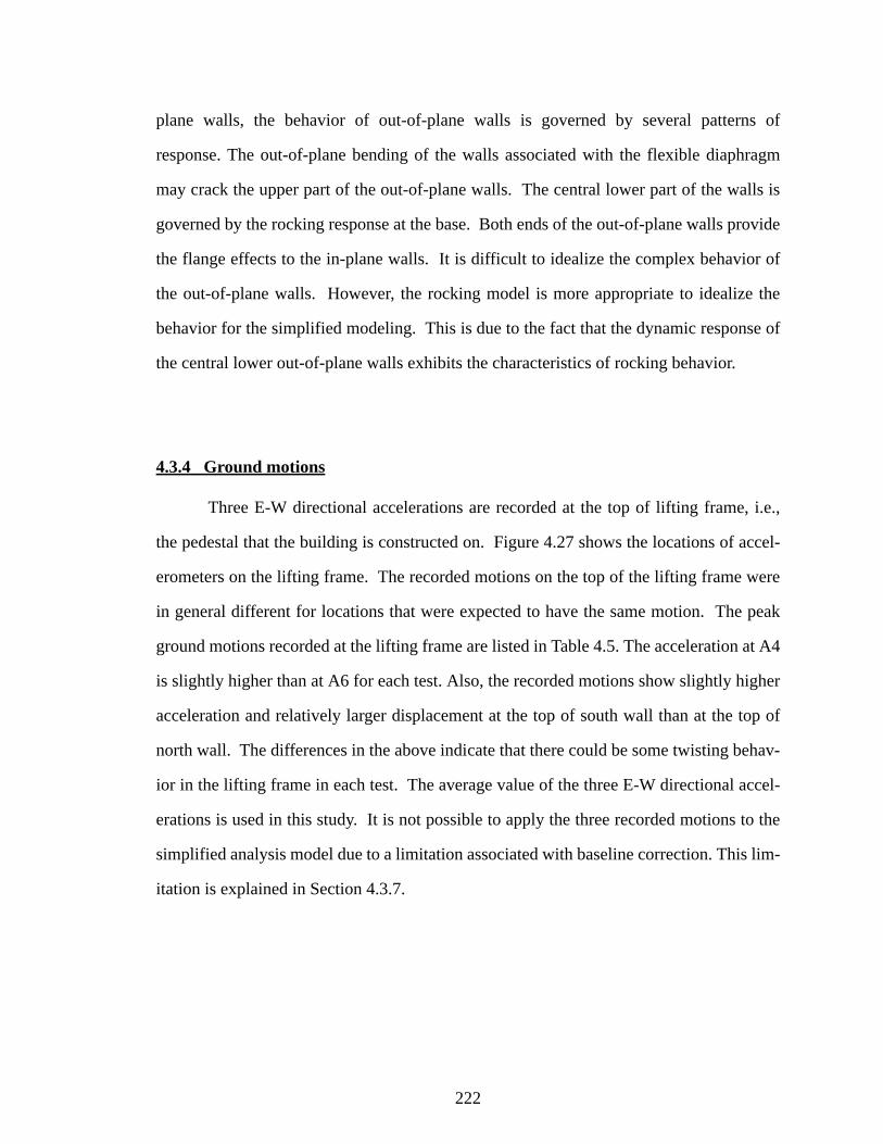
222

plane walls, the behavior of out-of-plane walls is governed by several patterns of

response. The out-of-plane bending of the walls associated with the flexible diaphragm

may crack the upper part of the out-of-plane walls. The central lower part of the walls is

governed by the rocking response at the base. Both ends of the out-of-plane walls provide

the flange effects to the in-plane walls. It is difficult to idealize the complex behavior of

the out-of-plane walls. However, the rocking model is more appropriate to idealize the

behavior for the simplified modeling. This is due to the fact that the dynamic response of

the central lower out-of-plane walls exhibits the characteristics of rocking behavior.

4.3.4 Ground motions

Three E-W directional accelerations are recorded at the top of lifting frame, i.e.,

the pedestal that the building is constructed on. Figure 4.27 shows the locations of accel-

erometers on the lifting frame. The recorded motions on the top of the lifting frame were

in general different for locations that were expected to have the same motion. The peak

ground motions recorded at the lifting frame are listed in Table 4.5. The acceleration at A4

is slightly higher than at A6 for each test. Also, the recorded motions show slightly higher

acceleration and relatively larger displacement at the top of south wall than at the top of

north wall. The differences in the above indicate that there could be some twisting behav-

ior in the lifting frame in each test. The average value of the three E-W directional accel-

erations is used in this study. It is not possible to apply the three recorded motions to the

simplified analysis model due to a limitation associated with baseline correction. This lim-

itation is explained in Section 4.3.7.

223

Figure 4.27: Instrument two corners and mid-frame in two directions for measuring horizontal acceleration at lifting frame.

Table 4.5: Measured E-W directional acceleration at lifting frame.

4.3.5 Mass

The masses are lumped at the corresponding degrees-of-freedom of the wall and

diaphragm element shown in Table 4.6 and Fig. 4.7. A density of 120 pcf for the masonry

wall and an uniform distributed load of 2.42 psf for the diaphragm are used. For the

lumped mass calculation, an effective thickness of 2.2 in, which accounts for the 3.5 in

hollow masonry units, is used for the calculation of the wall masses.

Instrument (Origi-nal Index)

Peak Acceleration (g)

Test 3 Test 5 Test 9

A4 (AY106) 0.5667 0.7989 1.1552

A5 (AY100) 0.5070 0.6536 0.9538

A6 (AY102) 0.5065 0.6371 0.9172

A5

A2

A6A4A1a A1b

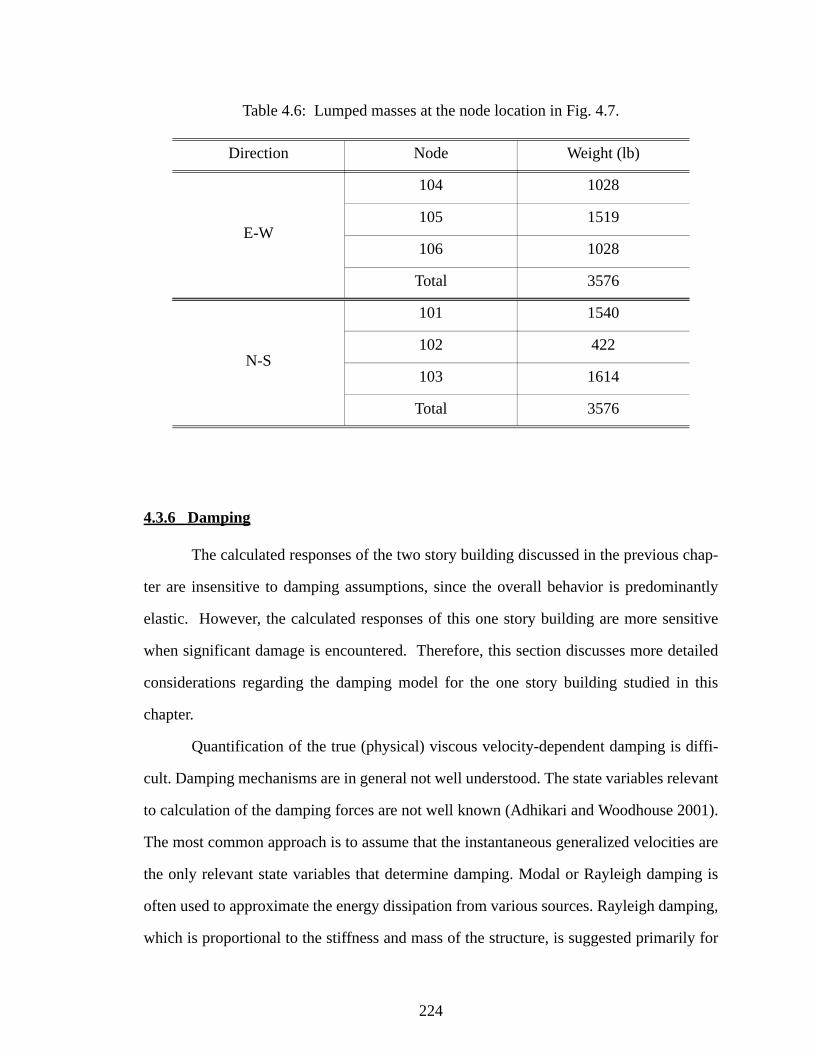
224

Table 4.6: Lumped masses at the node location in Fig. 4.7.

4.3.6 Damping

The calculated responses of the two story building discussed in the previous chap-

ter are insensitive to damping assumptions, since the overall behavior is predominantly

elastic. However, the calculated responses of this one story building are more sensitive

when significant damage is encountered. Therefore, this section discusses more detailed

considerations regarding the damping model for the one story building studied in this

chapter.

Quantification of the true (physical) viscous velocity-dependent damping is diffi-

cult. Damping mechanisms are in general not well understood. The state variables relevant

to calculation of the damping forces are not well known (Adhikari and Woodhouse 2001).

The most common approach is to assume that the instantaneous generalized velocities are

the only relevant state variables that determine damping. Modal or Rayleigh damping is

often used to approximate the energy dissipation from various sources. Rayleigh damping,

which is proportional to the stiffness and mass of the structure, is suggested primarily for

Direction Node Weight (lb)

E-W

104 1028

105 1519

106 1028

Total 3576

N-S

101 1540

102 422

103 1614

Total 3576

225

mathematical convenience (Adhikari and Woodhouse 2001). However, when structures

have nonproportional damping and/or exhibit nonlinear response, their response can not

be obtained by modal superposition. Therefore, strictly the damping can not be expressed

by modal damping ratios, but it must be expressed by an explicit damping matrix (Clough

and Penzien 1993). The concepts of hysteretic damping for nonlinear response and non-

proportional damping are discussed below.

Hysteretic damping for nonlinear analysis

To take into account the energy (or force) dissipation via inelastic response, it is

better to use hysteretic damping rather than viscous damping. However, it is difficult to

estimate the hysteretic damping factor of a building. In order to use hysteretic damping,

the nonlinear response of each structural component in the building, which indicates the

dissipation forces or the dissipated energy per cycle, should be measured by testing.

Therefore, hysteretic damping is difficult to consider in analysis modeling.

Nonproportional damping

In the analysis of a building made up of two types of materials (i.e., buildings with

flexible diaphragms and reinforced masonry walls), the two different materials provide

different energy dissipation (Clough and Penzien 1993).

The construction of the nonproportional damping matrix is similar to that in devel-

oping proportional damping matrices. Rayleigh damping coefficients, and , in Eq.

1.2 are determined for two damping ratios from linear analysis. The coefficients are given

by

(4.6)

a0 a1

a0a1

⎩ ⎭⎪ ⎪⎨ ⎬⎪ ⎪⎧ ⎫

2ωmωn

ωn2 ω– m

2--------------------- ωn ω– m

1 ωn⁄– 1 ωm⁄

ξmξn

⎩ ⎭⎪ ⎪⎨ ⎬⎪ ⎪⎧ ⎫

=

226

where, = damping ratio associated with the two specific frequencies, .

For , different Rayleigh coefficients and (see Eqs. 4.7 and 4.8)

are assigned to flexible diaphragms and reinforced masonry walls (Bathe 1996). These

coefficients depend on the frequencies determined by solving the eigenproblem of the

building using the combined initial elastic stiffness and mass matrices of masonry walls

and diaphragms (Clough and Penzien 1993). Thus the diaphragm and wall damping sub-

matrices are given by

(4.7)

(4.8)

When the nonproportional damping matrix of the structure is constructed as shown

in Fig. 4.28, the common DOFs (X in Fig. 4.28) include contributions from the diaphragm

and the wall damping matrices.

Figure 4.28: Assembly of combined damping matrices.

When the damping ratios and are known (or specified), the

simplest way to formulate a non-proportional damping matrix is to construct it by combin-

ing the proportional matrices developed for each diaphragm and wall using Eqs. 4.7 and

ξm ξ,n

ωm ω,n

ξwall ξdiaphragm≠ a0 a1

Cdiaphragm a0_diaphragmMdiaphragm a1_diaphragmKdiaphragm+=

Cwall a0_wallMwall a1_wallKwall+=

[C] =

Flexible DiaphragmCdiaphragm

WallCwall

X

ξwall ξdiaphragm

227

4.8 (see Fig. 4.28) (Clough and Penzien 1993). The damping model of the two-story

building discussed in the previous chapter does not consider the walls and the diaphragm

damping ratios separately. This is because the specific damping ratios of the wall and dia-

phragm applied to the two story building do not affect the calculated response signifi-

cantly due to its overall elastic behavior. However, the one-story building studied in this

chapter has significant damage in the latter tests, and therefore the non-proportional damp-

ing model is necessary to give results comparable to the observed response of the physical

structure.

The coefficients are calculated using the corresponding first and third modes (see

Fig. 4.29) because the analytical model has three degrees of freedom for the E-W and N-S

directions and the same damping ratio is desired approximately for the corresponding

three modes in the E-W direction, i.e., m = 1, and n = 3 in Eq. 4.6 (Chopra 1995). The

same damping ratios for the first and higher mode, i.e., are assumed to calcu-

late the Rayleigh damping coefficients for a practical linear analysis with proportional

damping matrix. Therefore, given the first ( ) and third frequencies ( ) calculated

from linear analysis of 75 and 141 rad/sec, respectively, and the same damping ratio of 3%

for the first and third modes is assumed to calculate the proportional damping matrix of

the diaphragm structure, the Rayleigh damping coefficients and are 2.932 and

0.000278 (see Fig. 4.30 to see the variation of damping ratio and frequency for Rayleigh

damping). If a damping ratio of 6% for the first and third modes is assumed to calculate

the proportional damping matrices of the walls, the Rayleigh damping coefficients and

are 5.864 and 0.000556. The coefficients for 6% damping are two times higher than

those for 3% damping. As shown in Fig. 4.29, the first mode shape is associated with the

diaphragm displacement and the second and third mode shapes are associated with the in-

plane wall displacements. When the damping ratios and are not same, the coeffi-

cients differ significantly from those calculated based on . If the damping ratio

of the first mode is 3% and the damping ratio of the third mode is 4%, the Rayleigh damp-

ξ1 ξ3=

ω1 ω3

a0 a1

a0

a1

ξm ξn

ξm ξn=

228

ing coefficients and are 1.832 and 0.000475, respectively. If the damping ratio of

the first mode is 3% and the damping ratio of the third mode is higher than 5.67%, the

coefficient will be a negative value and will be higher than 0.00166. Any non-

negative value of is a possible candidate for a damping model. Figure 4.30 summa-

rizes graphically the Rayleigh damping coefficients discussed above.

Figure 4.29: Eigenmode shapes of the building.

Figure 4.30: Variation of damping ratio and frequency for Rayleigh damping.

Recommended procedure for the MDOF models.

In this research, a nonproportional damping is used for linear and nonlinear analy-

a0 a1

a0 a1

a0

1st mode 2nd mode 3rd mode

0.00

0.05

0.10

0 100 200

ξ1 = ξ3 = 0.03a0 = 2.932, a1=0.000278

ξ1 = ξ3 = 0.06a0 = 5.864, a1=0.000556

ξ1 = 0.03, ξ3 = 0.0567a0= 0, a1=0.000803

ξ1 = 0.03, ξ3 = 0.04a0= 1.832, a1=0.000475

0.03

0.06

ξ

ω

229

sis. The proportional damping matrix is calculated for each of the parts because of the

resulting simplicity and computational advantages. Rayleigh damping is a velocity-depen-

dent damping. Therefore, it is necessary for structural engineer to pay attention to what

velocity (relative or absolute velocity) is used to solve the linear equation of motion

because some programs use absolute values. In the view of the authors, relative velocity is

a more appropriate choice to approximate the seismic responses of buildings. The Ray-

leigh damping coefficients are calculated from linear analysis and are used to approximate

unknown energy dissipation within the structure. The damping matrix for a structure

should be determined from its modal damping ratios estimated from available data.

The CERL personnel performed three sine-decay tests in the three principal direc-

tions (E-W, N-S and vertical direction) to estimate the equivalent viscous damping within

the elastic structure. The building was excited and abruptly halted to capture the decay of

the accelerations. An equivalent damping ratio of 3% was taken from the E-W directional

sine-decay test (Cohen 2001). However, it is possible that more than one damping ratio

may represent the system response equally well, so that an identified damping becomes

non-unique (Adhikari and Woodhouse 2001). It can be concluded that the assumption of

3% damping ratio is not appropriate for all the structural components of the building based

on the analysis results reported subsequently in this chapter.

Although the damping matrices do not strictly combine in the same way as the

stiffness matrices, the procedure illustrated in Fig. 4.28 is the simplest way to determine

the structure nonproportional damping matrix (Clough and Penzien 1993). For the simpli-

fied MDOF modeling of the building, the lumped masses of the analytical MDOF model

shown in Fig. 4.6 are associated with the common DOFs at the interface between the dia-

phragm and the wall elements (see Fig. 4.28). Although it is possible that more than one

damping ratio may represent the response of the building, the viscous Rayleigh damping

coefficients and are calculated from the equivalent damping

ratio of 3% taken from the E-W directional sine-decay test. The coefficient

a0_diaphragm a1_diaphragm

a0_diaphragm

230

is applied to the lumped masses. Thus, the damping contribution from the masses in Eqs.

4.7 and 4.8 are assumed to be equal (i.e. ) for simplicity.

When the effects of force loss and energy dissipation are assumed to be small, hys-

teretic damping of masonry walls can be approximately modeled as viscous damping with

an equivalent coefficient of viscous damping. In this work, the Rayleigh damping coeffi-

cient , which is proportional to stiffness, is calibrated to take into account the

energy dissipated by local damage within the wall during nonlinear time history analyses.

This procedure is discussed further in Section 4.4.

4.3.7 Difficulties of linear and nonlinear time history analysis

4.3.7.1 Baseline correction

The integration of the acceleration record through time may result in a relatively

large displacement at the end of the event when an acceleration history is specified for

analysis. This behavior typically occurs due to mechanical errors or an insufficient sam-

pling frequency such that the actual acceleration history is not accurately captured. To

compensate for these errors, a base line correction technique proposed by Newmark

(1973) can be applied to the ground motion for time history analysis (HKS 2000). How-

ever, when more than one ground motion is applied to the structure in a given direction, it

is not appropriate to correct the approximate acceleration histories by using the baseline

correction technique (i.e., different base excitation at each of the in-plane walls in the

CERL test structure).

The measured accelerations at the lifting frame in the E-W direction are not sym-

metrical as shown in Table 4.5. The peak acceleration at the corner of the lifting frame

below the south wall (0.56 g) is larger than that at the north corner and center of the lifting

frame (0.50 g). Figures 4.31 and 4.32 show the measured and calculated relative displace-

a0_wall a0_diaphragm=

a1_wall

231

ments, when three measured accelerations are applied to the bottom of the structures asso-

ciated with the measured location at the lifting frame. The calculated peak acceleration is

1.59 g compared to the measured acceleration, 1.60 g. Even though the comparison of the

three measured accelerations shows good comparative results in peak acceleration as

shown in Fig. 4.35, the relative displacement from 8 to 9 sec (see Fig. 4.32) is larger than

the measured one. The baseline correction method may not be used when different accel-

erations are applied to DOFs that have the same direction. In this study, this problem is

surmounted by using the average input acceleration in the E-W direction to represent the

test excitation in the analysis.

Figure 4.31: Recorded relative displacement at the center of the diaphragm.

Figure 4.32: Calculated relative displacement at the center of the diaphragm applying three measured acceleration at the lifting frame.

-0.15-0.1

-0.050

0.050.1

0.15

0 1 2 3 4 5 6 7 8 9Time (sec)

Dis

plac

emen

t (in

)

-0.20

-0.10

0.00

0.10

0.20

0 1 2 3 4 5 6 7 8 9Time (sec)

Dis

plac

emen

t (in

)

232

4.3.7.2 Time step

The issue of choosing suitable time steps is a difficult problem to resolve in the

case of linear and nonlinear dynamic analysis. The recorded incremental time step in the

physical test is 0.005 sec. In the analysis model, it is always necessary to provide suitable

steps to allow an acceptable level of accuracy. In order to insure accurate representation

of the effects of this discretized time history, the time step must be smaller than 0.005 sec.

Figure 4.33 shows the comparison of measured and calculated accelerations at the center

of the diaphragm based on three different time steps of 0.005, 0.0025, and 0.001 sec.,

respectively, in the time history analyses. The differences in the results of the analyses

with increments of 0.005 and 0.0025 sec. are much larger than that between those 0.0025

and 0.001sec. Thus, for the consistent linear and nonlinear dynamic analyses, a time step

of 0.0025 sec. is used for linear analysis, and a time step of 0.001 sec. is used for non-lin-

ear dynamic analysis.

Figure 4.33: 1/2 second comparison of measured and calculated history varying time step from 0.005sec to 0.001sec.

-2

-1.5

-1

-0.5

0

0.5

1

1.5

4.5 4.6 4.7 4.8 4.9

Time (sec)

Acc

eler

atio

n (g

)

Measured Time step = 0.005 sec

Time step = 0.0025 sec Time step = 0.001 sec

233

4.4 Calibration of analytical model based on shaking table test results

The test building is idealized using the simplified multi-degree-of-freedom

(MDOF) approach discussed in Section 4.3.1. The diaphragm element properties are

obtained from the experimental diaphragm test results discussed in Section 4.3.2. How-

ever, it is difficult to estimate the response characteristics of masonry in-plane and out-of-

plane walls, as discussed in Section 4.1. The calibration process is targeted at determining

in-plane and out-of-plane wall stiffnesses, strengths, and damping.

The model calibration process (see Fig. 4.34) is applied to predict the system prop-

erties, which involve complex interactions between the in-plane wall, out-of-plane wall

and diaphragm DOFs. The model calibration procedure is based on comparison of analyt-

ical model predictions to the shaking table test results. The studies focus on the accelera-

tion and displacement in the E-W direction at the top of the south and north walls (nodes

104 and 106 in Fig. 4.6) and at the center of the roof diaphragm (node 105 in Fig. 4.6).

Key unknown wall parameters are varied and examined in each analysis until good com-

parisons are achieved. The comparison includes the peak response and the history of the

responses throughout the tests. The detailed process is discussed in Sections 4.4.1 to 4.4.3.

Section 4.4.1 presents the linear analysis step of the model calibration (see Fig.

4.34) to determine the wall stiffness. The results of Test 3 from (Cohen 2001) are used to

identify the in-plane and out-of-plane wall stiffness. In Section 4.4.2, the results of Test 5

from (Cohen 2001) are used to capture the strength of the walls. In Section 4.4.3, Tests 9

and 10 from (Cohen 2001) are used to assess the hysteresis of the structural elements for

the nonlinear time history analysis.

234

Figure 4.34: Model calibration process used for wall properties.

4.4.1 Calibration of in-plane and out-of-plane wall initial stiffness using PGA = 0.5g

The first step of the model calibration process shown in Fig. 4.34 is applied to find

the elastic stiffness of in-plane and out-of plane walls. The peak acceleration of the input

ground motion of Test 3 is 0.5 g. This input motion, selected from the Carbondale suite

Step 1: Linear Analysis of Test 3 (No damage) - Determine Stiffness

Refined model Time historyanalysis

Modify initial stiffnessesFrequency analysisOriginalmodel

Compareresponses

Step 2: Nonlinear Analysis of Test 5 (Slight damage) - Determine Strength

Refined model Time historyanalysis

Modify strength

Compareresponses

Step 3: Nonlinear Analysis of Tests 9 & 10 (Extensive damage) - Determinehysteresis curves

Refined model Time historyanalysis

Modify hysteresis curve and postelastic tangent stiffness

Compareresponses

KF

∆

FyKF

∆

F

∆

End

O.K

O.K

O.K

235

(Wen and Wu 1999), is the modified record with its acceleration ordinates scaled by 75%.

Test 3 provides the basis for the linear analysis model because there was no damage dur-

ing the test. (see Table 4.1) (Cohen 2001).

The in-plane stiffnesses of the north and south walls is assumed initially as 40

kips/in, which is calculated using Eq. 2.72. During this calibration process, the in-plane

stiffness is increased from this initial values and the out-of-plane wall stiffness is

increased from zero. At each iteration of the calibration process, the Rayleigh damping

coefficients are recalculated using the results of the frequency analysis with the modified

stiffness values. The initial in-plane and out-of-plane stiffnesses are determined by com-

paring the overall history of the measured and calculated responses.

Section 4.4.1.1 summaries the peak measured responses of Test 3. Section 4.4.1.2

presents the predicted stiffness values obtained from this calibration. Section 4.4.1.3

shows the comparison of the measured and predicted responses.

4.4.1.1 Measured responses

Table 4.7 summarizes the peak measured responses corresponding to the locations

shown in Fig. 4.4. The complete measured time history responses are plotted in Figs. C.5

through C.16 of Appendix C. The peak acceleration and displacement at the center of the

diaphragm are 1.60 g and 0.12 in, respectively. The difference between the measured north

(0.72 g) and south wall (0.78 g), shown in Table 4.7, may be attributed to experimental

errors in the lifting frame, as discussed in Section 4.3.4. The measured acceleration at the

top of south wall is 0.06 g higher than that of north wall. The relative peak displacements

of the top of the north and south walls are 0.026 in.

236

Table 4.7: Summary of measured accelerations and displacement in the E-W direction.

4.4.1.2 Summary of predicted properties

The predicted properties from Step 1 are summarized in Table 4.8. The predicted

in-plane and out-of-plane wall stiffnesses are 50 kips/in and 16 kips/in, respectively. The

predicted in-plane wall stiffness of 50 kips is higher than the stiffness of 40 kips/in calcu-

lated by using the simplified mechanics of materials types of approach without consider-

ing the flange effects from the out-of-plane walls and without reinforcing bar (see Table

4.4). The difference, 10 kips/in, may be attributed to the flange effects from the east and

west walls or reinforcement. The predicted in-plane stiffness is similar to the in-plane

stiffness with reinforcement and without flange, 53 kips/in, summarized in Table 4.3.

The estimated total lateral stiffness of Cohen’s two DOF model was 320 kips/in

(Cohen 2001). This total lateral stiffness of the test building is bigger than that (257 kips/

in) of FEA analysis with rigid diaphragm shown in Fig. 4.25 (b). However, the total lateral

stiffness of the shear wall building must be smaller than 257 kips/in due to the flexibility

of the diaphragm. The total lateral stiffness from this calibrations process is 23 kips/in

obtained as the sum of the in-plane and out-of-plane stiffnesses shown in Table 4.8. Based

on these estimated stiffnesses, the detailed comparisons of measured and calculated

responses are summarized in Section 4.4.1.3.

LocationPeak Acceleration (g) Peak displacement (in)

Instrument Test 3 Instrument Test 3

South wallA104a 0.7363

D104 0.026A104b 0.7756

Diaphragm A105 1.6002 D105 0.120

North wallA106a 0.7162

D106 0.026A106b 0.6922

237

Table 4.8: Predicted properties from Step 1.

4.4.1.3 Comparison between measured and calculated responses

Of the two recorded accelerations, the one that has larger peak value is selected to

compare with the analysis results. Table 4.9 summarizes the comparison of the measured

and calculated response of the structure using the two damping ratios for the masonry

walls and the diaphragm (see Section 4.3.6).

The measured fundamental period of the structure was 0.07sec. The fundamental

period obtained in this study is 0.08 sec. The period of 0.10 sec for the two DOF model

developed by (Cohen 2001) is slightly higher than the measured period. The first ( )

and third frequencies ( ) are 75 and 141 rad/sec, respectively. As discussed in Section

4.3.6, 3% damping is used to calculate Rayleigh damping coefficients for the diaphragm.

The Rayleigh damping coefficients and of the lumped masses at

the common DOFs (X in Fig. 4.28) are 2.932. Two different damping ratios (3% and 10%)

are used to calculate the Rayleigh damping coefficients of the in-plane masonry

walls for investigating the effect of the damping ratio within the masonry walls. The

damping coefficients are 0.00028 and 0.00097 for the damping ratios of 3% and

10%, respectively. The damping coefficient of out-of-plane wall is 0.00028.

Component Stiffness

In-plane Walls 50 kips/in

Out-of-plane Wall 16 kips/in (=East + West Wall)

Equivalent diaphragm stiffness (Get)1 8.82 kips/in (see Section 4.3.2.2)

ω1

ω3

a0_wall a0_diaphragm

a1_wall

a1_wall

a1_wall

238

Table 4.9: Comparison of measured and calculated response using PGA = 0.5 g.

The reason for showing the results of two damping ratios in Table 4.9 is the con-

sideration of the subsequent nonlinear time history analysis of the building, as discussed in

Section 4.3.6. The comparison of the analyses using two different damping ratios shows

that the linear responses of the building are not sensitive to this variable. The change in the

damping ratio doesn’t significantly affect the displacement and acceleration at the center

of the diaphragm, as shown in Figs. 4.40 and 4.45 and Table 4.9. The change from 3% to

10% damping slightly decreases the calculated peak response of in-plane walls, as shown

in Table 4.9. However, when the in-plane wall is damaged, the effects of damping will be

significant for the strong excitation of Tests 9 and 10 (see Section 4.4.3.3).

The peak acceleration, 1.48 g, at the center of the diaphragm is slightly smaller

than the measured acceleration, 1.60 g, due to the average input motion discussed in Sec-

Compared Item Measured

Calculated

Refined FEM model (Cohen 2001)

2-DOF RSA

(Cohen 2001)

MDOF model

Damping ξdia = 3% ξwall = 3%

Damping ξdia = 3% ξwall=10%

Fundamental Fre-quency

14 Hz (0.07sec)

12 Hz (0.08 sec)

10.5 Hz (0.10sec) 12 Hz (0.08 sec)

Diaphragm deflection - - - 0.096 in 0.093 in

Center of diaphragm

(105)

Acc. 1.6 g 1.8 g 1.5 g 1.48 g 1.45 g

Disp. 0.12 in 0.13 in 0.15 in 0.11 in 0.10 in

North wall (106)

Acc. 0.72 g

- -

0.86 g 0.70 g

Disp. 0.026 in 0.022 in 0.020 in

South wall (104)

Acc. 0.78 g 0.86g 0.70g

Disp. 0.026 in 0.022 in 0.020 in

239

tion 4.3.7.1. As discussed in Section 4.3.7.1, the peak acceleration of the average ground

motion (0.53g) is smaller than the measured peak acceleration at the bottom of south wall

(0.57g) (see Table 4.5). When the three different input accelerations measured at the base

of north and south walls and at the center of the lifting frame shown in Table 4.5 are used

in this analysis, the peak acceleration is changed from 1.48 g to 1.53 g, as shown in Fig.

4.35. Therefore, it is concluded that the increased acceleration (1.53g) is due to the input

ground motion. This trend appears to result from the fact that the measured acceleration at

the center of the diaphragm is dynamically amplified due to the input accelerations. The

three different input motions are not used in this model calibration process due to the lim-

itation of the baseline correction discussed in Section 4.3.7.1. However, the difference

compared to the measured peak value is acceptable, since the behavior of the test building

is predominantly symmetric and each portion of the overall time history curve matches

well without any shift phase, as shown in Figs. 4.35 and 4.39.

The calculated displacement at the center of the diaphragm is 0.11 in compared to

the measured value of 0.12 in (see Table 4.9). Due to the average input ground motion dis-

cussed above, the calculated responses are slightly smaller than the measured responses.

Figures 4.41 and 4.44 show the comparison of the measured and calculated relative dis-

placement at the center of the diaphragm.

240

Figure 4.35: 0.3 second comparisons of measured and calculated response (Damping: ξdia = 3%, ξwall = 3%).

Figure 4.36: Measured acceleration at the center of the diaphragm employed in the analysis with PGA =0.5g.

-1.6

-1.2

-0.8

-0.4

0.0

0.4

0.8

1.2

4 4.1 4.2 4.3

Time (sec)

Acc

eler

atio

n (g

)

Measured

Input motion: Three measured acclerations at the lifting frameInput motion: Modified average acceleration at the lifting frame

-1.2

-1.0

-0.8

-0.6

-0.4

-0.2

0.0

0.2

0.4

0.6

0.8

1.0

5.5 5.6 5.7 5.8

Time (sec)A

ccel

erat

ion

(g)

-2.0-1.5-1.0-0.50.00.51.01.52.0

0 1 2 3 4 5 6 7 8 9Time (sec)

Acce

lera

tion

(g)

Measured

241

Figure 4.37: Calculated acceleration at the center of the diaphragm applying the average acceleration employed in the analysis with PGA =0.5g (Damping: ξdia = 3%, ξwall = 3%).

Figure 4.38: Calculated acceleration at the center of the diaphragm applying the average acceleration employed in the analysis with PGA =0.5g (Damping: ξdia =3%, ξwall = 10%).

Figure 4.39: Two-second comparison of acceleration at the center of the diaphragm applying the average acceleration with PGA = 0.5g (Damping: ξdia = 3%, ξwall = 3%).

-2.0-1.5-1.0-0.50.00.51.01.52.0

0 1 2 3 4 5 6 7 8 9Time (sec)

Acce

lera

tion

(g)

Calculated

-2.0-1.5-1.0-0.50.00.51.01.52.0

0 1 2 3 4 5 6 7 8 9Time (sec)

Acc

eler

atio

n (g

) Calculated

-2-1.5

-1-0.5

00.5

11.5

4 4.2 4.4 4.6 4.8 5 5.2 5.4 5.6 5.8 6Time (sec)

Acc

eler

atio

n (g

)

Measured Calculated

242

Figure 4.40: Two-second comparison of acceleration at the center of the diaphragm applying the average acceleration with PGA = 0.5g (Damping: ξdia = 3%, ξwall = 10%).

Figure 4.41: Measured displacement at the center of the diaphragm for Test 3 with PGA = 0.5g.

Figure 4.42: Calculated displacement at the center of the diaphragm for Test 3 with PGA = 0.5g. (Damping: ξdia = 3%, ξwall = 3%).

-2-1.5

-1-0.5

00.5

11.5

4 4.2 4.4 4.6 4.8 5 5.2 5.4 5.6 5.8 6Time (sec)

Acc

eler

atio

n (g

)Measured Calculated

-0.15-0.10

-0.050.00

0.05

0.10

0.15

0 1 2 3 4 5 6 7 8 9Time (sec)

Dis

plac

emen

t (in

) Measured

-0.15

-0.10

-0.05

0.00

0.05

0.10

0.15

0 1 2 3 4 5 6 7 8 9Time (sec)

Dis

plac

emen

t (in

) Calculated

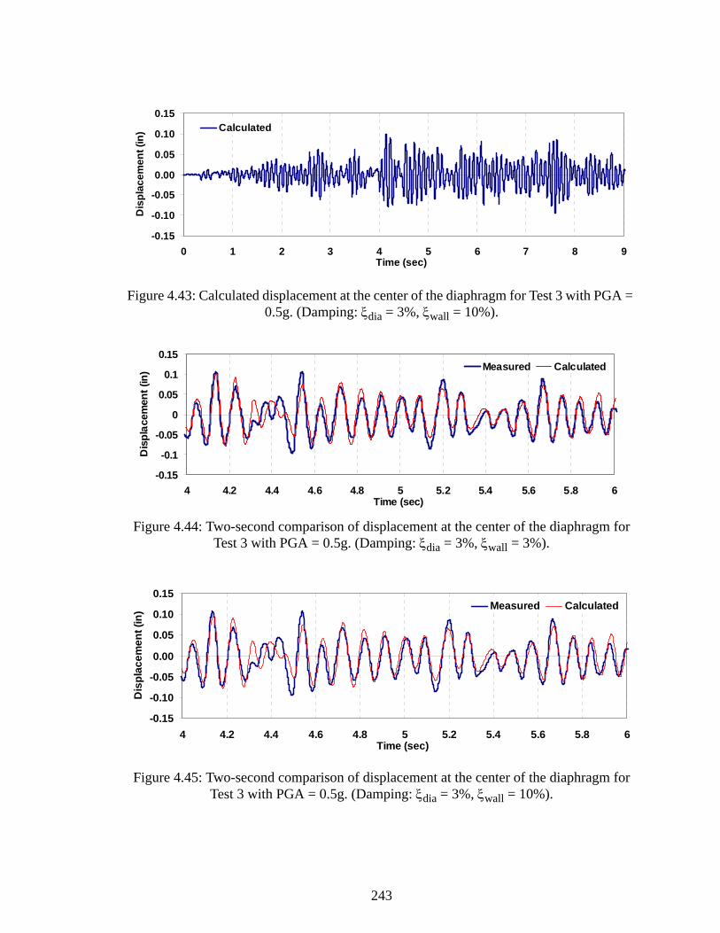
243

Figure 4.43: Calculated displacement at the center of the diaphragm for Test 3 with PGA = 0.5g. (Damping: ξdia = 3%, ξwall = 10%).

Figure 4.44: Two-second comparison of displacement at the center of the diaphragm for Test 3 with PGA = 0.5g. (Damping: ξdia = 3%, ξwall = 3%).

Figure 4.45: Two-second comparison of displacement at the center of the diaphragm for Test 3 with PGA = 0.5g. (Damping: ξdia = 3%, ξwall = 10%).

-0.15

-0.10

-0.05

0.00

0.05

0.10

0.15

0 1 2 3 4 5 6 7 8 9Time (sec)

Dis

plac

emen

t (in

) Calculated

-0.15

-0.1

-0.05

0

0.05

0.1

0.15

4 4.2 4.4 4.6 4.8 5 5.2 5.4 5.6 5.8 6Time (sec)

Dis

plac

emen

t (in

) Measured Calculated

-0.15

-0.10

-0.05

0.00

0.05

0.10

0.15

4 4.2 4.4 4.6 4.8 5 5.2 5.4 5.6 5.8 6Time (sec)

Dis

plac

emen

t (in

) Measured Calculated

244

Effects of out-of-plane walls

When the out-of-plane wall is removed, the peak acceleration at the center of dia-

phragm is changed to 1.59 g (see Figs. 4.46 to 4.47), and the overall responses are also

changed (see Figs. 4.48 to 4.49). This acceleration are not changed considerably compared

to the computed value of 1.48 g given in the previous section, but the peak displacement

(0.385 in) is 3 times larger than the previously calculated value of 0.11 in. It is concluded

that the contribution of the out-of-plane wall in this type of building is important to reduce

the diaphragm deflection. A detailed sensitivity analysis of the effect of the out-of-plane

walls is discussed in Section 4.5.3.

Figure 4.46: Comparison of acceleration at the center of the diaphragm without the out-of-plane wall for PGA = 0.5g. (Damping: ξdia = 3%, ξwall = 3%).

Figure 4.47: Two second comparison of acceleration at the center of the diaphragm without the out-of-plane wall for PGA = 0.5g. (Damping: ξdia = 3%, ξwall = 3%).

-2-1.5

-1-0.5

00.5

11.5

2

0 1 2 3 4 5 6 7 8 9Time (sec)

Acc

eler

atio

n (g

) Measured Calculated

-2-1.5

-1-0.5

00.5

11.5

2

4 4.2 4.4 4.6 4.8 5 5.2 5.4 5.6 5.8 6Time (sec)

Acc

eler

atio

n (g

) Measured Calculated

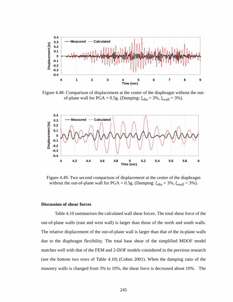
245

Figure 4.48: Comparison of displacement at the center of the diaphragm without the out-of-plane wall for PGA = 0.5g. (Damping: ξdia = 3%, ξwall = 3%).

Figure 4.49: Two second comparison of displacement at the center of the diaphragm without the out-of-plane wall for PGA = 0.5g. (Damping: ξdia = 3%, ξwall = 3%).

Discussion of shear forces

Table 4.10 summarizes the calculated wall shear forces. The total shear force of the

out-of-plane walls (east and west wall) is larger than those of the north and south walls.

The relative displacement of the out-of-plane wall is larger than that of the in-plane walls

due to the diaphragm flexibility. The total base shear of the simplified MDOF model

matches well with that of the FEM and 2-DOF models considered in the previous research

(see the bottom two rows of Table 4.10) (Cohen 2001). When the damping ratio of the

masonry walls is changed from 3% to 10%, the shear force is decreased about 10%. The

-0.4-0.3-0.2-0.1

00.10.20.30.4

0 1 2 3 4 5 6 7 8 9Time (sec)

Dis

plac

emen

t (in

) Measured Calculated

-0.4-0.3-0.2-0.1

00.10.20.30.4

4 4.2 4.4 4.6 4.8 5 5.2 5.4 5.6 5.8 6Time (sec)

Dis

plac

emen

t (in

) Measured Calculated

246

in-plane wall strengths estimated using the mechanics of materials type equations from

FEMA 356 (ASCE 2000a) and ACI 530-99 (MSJC 1999b) are summarized in Table 4.3.

The calculated in-plane wall shear forces (1.08 and 0.91 kips in Table 4.10) are smaller

than the flexural cracking force (1.3 kips shown in Table 4.3). However, the out-of plane

wall shear force, 1.6 kips, is higher than the estimated flexural cracking force (0.69 kips

shown in Section 4.3.3.3) and the yielding force (1.42kips) of the out-of-plane wall.

However, there is no observed damage during this test.

Table 4.10: Calculated shear force at the base using PGA = 0.5 g.

The diaphragm shear forces are summarized in Table 4.11. Using the MDOF

model, the diaphragm shear at both ends is 335 lb, and the shear force contribution from

the out-of-plane walls is 1,618 lb. The shear force and displacement calculated from the

two DOF model (Cohen 2001) is much higher than those of the refined FEM model devel-

oped by (Cohen 2001) and the MDOF model proposed in this research. The effects of out-

of-plane wall were not considered in the two DOF model.

Element

Shear force (lb)

Damping ξdia = 3% ξwall

= 3%

Damping ξdia = 3% ξwall=10%

1.South wall 1,078 913

2.North wall 1,078 913

3.out-of-plane wall (= East + West wall) 1,618 1,608

Total Base Shear

MDOF model(=1+2+3) 3,774 3,434

FEM model (Cohen 2001) 3,600

2-DOF model (Cohen 2001) 3,700

247

Table 4.11: Calculated shear force at the roof diaphragm level (ξdia and ξwall = 3%).

4.4.2 Calibration of out-of-plane wall strength using PGA = 0.67g

The second step of the model calibration process shown in Fig. 4.34 is applied to

find the strength of out-of plane walls. The peak acceleration of the input ground motion

of Test 5 is 0.67 g. Test 5 provides the basis for the nonlinear analysis model because there

was slight cracking in east and west walls during the test. (see Table 4.1) (Cohen 2001).

As shown in Fig. 4.6, the out-of-plane of east and west walls are modeled by a sin-

gle wall element. During this calibration process, the total out-of-plane strength of east

and west walls is determined from the estimated flexural cracking force Vcr (0.691 kips)

(see Section 4.3.3.3). The initial stiffnesses of the in-plane and out-of-plane walls pre-

dicted from the previous step (see Section 4.4.1) are used in this step. The total strength of

out-of-plane walls is determined by comparing the overall history of the measured and

calculated responses.

Section 4.4.2.1 summarizes the peak measured responses of Test 5. Section 4.4.2.2

presents the predicted strength values obtained from this calibration. Section 4.4.2.3

shows the comparison of the measured and predicted responses.

Element Shear Force

Overall drift ratio at the center of dia-

phragm

a. Diaphragm shear 335 lb 0.074% (Diaphragm Drift)

b. Out-of-plane wall 1,618 lb 0.13% (0.11 in)

Dia-phragm shear

MDOF model (=2*a +b) 2,288 lb 0.13% (0.11 in)

Refined FEM model (Cohen 2001) 2,500 lb 0.15% (0.128 in)

2-DOF Response Spectrum Analysis model (Cohen 2001) 3,200 lb 0.18% (0.148 in)

248

4.4.2.1 Measured responses

Table 4.12 summarizes the peak measured response corresponding to the location

shown in Fig. 4.4. The complete measured history responses are plotted in Figs. C.17

through C.30 in Appendix C. The peak acceleration and displacement at the center of the

diaphragm are 2.51 g and 0.225 in, respectively. The difference between the measured

north (0.87g) and south wall (0.97g) shown in Table 4.12, may be attributed to experi-

mental errors in the lifting frame, as discussed in Section 4.3.4. The measured acceleration

at the top of south wall is 0.1 g higher than that of north wall.

Table 4.12: Summary of measured accelerations and displacement in the E-W direction.

The measured peak relative displacements at the top of north and south wall are

0.028 in and 0.036 in, respectively. The relative peak displacement at the center of the dia-

phragm associated with the out-of-plane wall displacement is 0.225 in. The peak in-plane

and out-of-plane wall displacements show 39% and 88% increase, respectively, over the

measured responses of Test 3.

LocationPeak Acceleration (g) Peak displacement (in)

Instrument Test 5 Instrument Test 5

South wallA104a 0.9501

D104 0.036A104b 0.9752

Diaphragm A105 2.5121 D105 0.225

North wallA106a 0.8665

D106 0.028A106b 0.8666

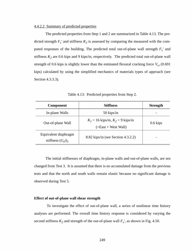
249

4.4.2.2 Summary of predicted properties

The predicted properties from Step 1 and 2 are summarized in Table 4.13. The pre-

dicted strength Fs' and stiffness K2 is assessed by comparing the measured with the com-

puted responses of the building. The predicted total out-of-plane wall strength Fs' and

stiffness K2 are 0.6 kips and 9 kips/in, respectively. The predicted total out-of-plane wall

strength of 0.6 kips is slightly lower than the estimated flexural cracking force Vcr (0.691

kips) calculated by using the simplified mechanics of materials types of approach (see

Section 4.3.3.3).

Table 4.13: Predicted properties from Step 2.

The initial stiffnesses of diaphragm, in-plane walls and out-of-plane walls, are not

changed from Test 3. It is assumed that there is no accumulated damage from the previous

tests and that the north and south walls remain elastic because no significant damage is

observed during Test 5.

Effect of out-of-plane wall shear strength

To investigate the effect of out-of-plane wall, a series of nonlinear time history

analyses are performed. The overall time history response is considered by varying the

second stiffness K2 and strength of the out-of-plane wall Fs', as shown in Fig. 4.50.

Component Stiffness Strength

In-plane Walls 50 kips/in -

Out-of-plane Wall K1 = 16 kips/in, K2 = 9 kips/in

(=East + West Wall)0.6 kips

Equivalent diaphragm stiffness (Get)1

8.82 kips/in (see Section 4.3.2.2) -

250

The shear strength, Fs' in Figs. 4.50 and 4.52, is the point where stiffness changes

in the bi-linear curve. The K2 stiffness (9 kips/in) is also found from the sensitivity analy-

sis varying the shear strength of the out-of-plane wall. Figures 4.50 to 4.52 show the

effect of the bi-linear curve in Figs. 4.50 and 4.51. As the out-of-plane wall shear strength

is decreased from 1.0 to 0.9 kips, the acceleration and out-of-plane displacement at the

center of the diaphragm is not changed significantly as shown in Figs. 4.50 and 4.51. In

this range of the out-of-plane wall shear strength, the diaphragm is predominantly elastic

as shown in Fig. 4.52. When the shear strength is changed from 0.8 to 0.6 kips, the

responses of acceleration and displacement at the center of the diaphragm match well with

the measured ones, as shown in Figs. 4.50 and 4.51. Therefore, as the shear strength is

decreased from 0.8 to 0.6 kips, the diaphragm begins to show inelastic behavior (see Fig.

4.52). In the range between the shear strengths of 0.6 and 0.4 kips, the response is not

largely changed. Based on this sensitivity analysis, the out-of-plane wall strength, Fs', and

tangent stiffness, K2 are predicted as 0.6 kips and 9 kips/in, respectively.

251

Figure 4.50: 0.15 second comparison of accelerations at the center of the diaphragm with changing Fs' in the bi-linear curve (K1 = 16kips/in, K2 = 9kips/in, Damping: ξdia = 3%,

ξwall = 3%).

Figure 4.51: 0.15 second comparison of displacements at the center of the diaphragm with changing Fs' in the bi-linear curve (K1 = 16kips/in, K2 = 9kips/in, Damping: ξdia = 3%,

ξwall = 3%).

-3

-2

-1

0

1

2

4.55 4.6 4.65 4.7Time (sec)

Acc

eler

atio

n(g)

Measured

Fs' = 0.4 kips Fs' = 0.5 kips

Fs' = 0.6 kips Fs' = 0.7 kips Fs' = 0.8 kips

Fs' = 0.9 kips Fs' = 1.0 kips

K1

K2Fs'F

∆Fs'=0.6kips

Fs'=1.0kips

-0.25

-0.15

-0.05

0.05

0.15

0.25

4.55 4.6 4.65 4.7Time (sec)

Dis

plac

emen

t (in

)

Measured Fs' = 0.4 kips

Fs' = 0.5 kips Fs' = 0.6 kips

Fs' = 0.7 kips Fs' = 0.8 kips

Fs' = 0.9 kips Fs' = 1.0 kips

K1

K2Fs'F

∆

Fs'=0.4kips

Fs'=1.0kips

252

Figure 4.52: The diaphragm response with changing the out-of-plane wall shear strengths (K1 = 16kips/in, K2 = 9kips/in, Damping: ξdia = 3%, ξwall = 3%).

0.1

0.15

0.2

0.25

0.3

0.4 0.6 0.8 1

Out-of-plane Wall Fs' (kips)

Out

-of-p

lane

Wal

l Dri

ft R

atio

(%

)

-0.7

-0.35

0

0.35

0.7

-0.2 0.0 0.2

Diaphragm Drift Ratio (%)

Diap

hrag

m S

hear

For

ce

(kip

s)

Fs' = 0.4 kips

-0.7

-0.35

0

0.35

0.7

-0.2 0.0 0.2

Diaphragm Drift Ratio (%)

Dia

phra

gm S

hear

For

ce

(kip

s)

Fs' = 1.0 kips

-0.7

-0.35

0

0.35

0.7

-0.2 -0.1 0.0 0.1 0.2

Diaphragm Drift Ratio (%)

Dia

phra

gm S

hear

For

ce

(kip

s)

Fs' = 0.8 kips

-0.7

-0.35

0

0.35

0.7

-0.2 -0.1 0.0 0.1 0.2

Diaphragm Drift Ratio (%)

Dia

phra

gm S

hear

For

ce

(kip

s)

Fs' = 0.7 kips

-0.7

-0.35

0

0.35

0.7

-0.2 0.0 0.2

Diaphragm Drift Ratio (%)

Diap

hrag

m S

hear

For

ce

(kip

s)

Fs' = 0.6 kips

253

4.4.2.3 Comparison between measured and calculated responses

Table 4.14 summarizes the comparison of the measured and calculated responses

of the structure using the two damping ratios for the masonry walls and the diaphragm

(see Section 4.3.6). The change in the damping ratio doesn’t significantly affect the dis-

placement and acceleration at the center of the diaphragm due to the slight damage of the

out-of-plane walls. When 10% damping is used for the in-plane walls, the calculated

responses at the center of the diaphragm are slightly increased and the ones at the top of

in-plane walls are decreased compared to the 3% damping.

Table 4.14: Comparison of measured and calculated response using PGA = 0.67 g.

The measured fundamental period of Test 5 is increased to 0.077 sec compared to

that of Test 3 (see Table 4.9). However, the calculated fundamental period (0.08 sec) is not

changed due to the same elastic properties of the MDOF model used in the analysis model

Compared Item Measured

Calculated (MDOF model)

Damping ξdia = 3% ξwall = 3%

Damping ξdia = 3% ξwall=10%

Fundamental Frequency 13 Hz (0.077 sec)

12 Hz (0.08 sec)

Diaphragm deflection - 0.20 in 0.22 in

Center of dia-phragm (105)

Acceleration 2.51g 2.22 g 2.32 g

Displacement 0.23 in 0.22 in 0.23 in

North wall (106)Acceleration 1.0g 1.2 g 1.0 g

Displacement 0.036 in 0.032 in 0.026 in

South wall (104)Acceleration 0.82g 1.2g 1.0g

Displacement 0.028 in 0. 032 in 0. 026 in

254

of Test 3 (see Section 4.4.1.2). The Rayleigh damping coefficients of the diaphragm and

in-plane walls used in Step 1 (see Section 4.4.1.3) are not changed. The damping coeffi-

cient ( ) of the out-of-plane wall is reduced to 0.0001 to match the measured peak

relative displacement and acceleration at the center of the diaphragm. Figure 4.53 summa-

rizes the Rayleigh damping coefficients used in constructing the non-proportional damp-

ing matrix. The coefficient is varied to investigate the effects of the stiffness

proportional part of the damping matrix. The out-of-plane wall damping coefficients

of 0.0001 to 0.00097 correspond to damping ratios of 1% to 10%, respectively.

The Rayleigh damping curves obtained by varying from 0.00028 to 0.00097 are

between the 3% and 10% damping curves. Three different out-of-plane wall damping

coefficients are considered in Fig. 4.53 and are discussed below.

Figure 4.53: Summary of Rayleigh damping coefficients.

Figures 4.54 through 4.57 present the effects of the stiffness proportional damping

coefficient a1 of the out-of-plane wall. The overall phases of the calculated time history

a1_wall

a1_wall

a1_wall

a1_wall

ξ

ω

Diaphragmξ1 = ξ3 = 3%(a0 = 2.932, a1=0.000278)

ξ1 = ξ3 = 10%a0 = 8.878, a1=0.00097

In-plane walls(a0 = 2.932, a1=0.00097)

Out-of-plane wallsa0 = 2.932, a1=0.00097

a0 = 2.932, a1=0.00028a0 = 2.932, a1=0.00010

0 100 20065 1410.00

0.05

0.10

0.15

0.20

0.03

255

responses match well with the measured ones in these figures. However, when a damping

ratio of 10% ( ) is used for the out-of-plane wall, the peak relative

displacement and acceleration at the center of the diaphragm (0.17 in and 1.72 g, respec-

tively) are smaller than the measured ones (0.22 in and 2.51g, respectively) (see Fig. 4.54

(d) and 4.55 (d)). When the damping coefficient ( ) based on the

damping ratio of 3% is used, the peak relative displacement and acceleration at the center

of the diaphragm are 0.22 in and 2.21 g, respectively. A possible cause of the above differ-

ences may be an increase in the effective damping ratio in the damaged out-of-plane walls,

since the response of the out-of-plane walls is associated with the response at the center of

the diaphragm. When the damping coefficient ( ) is used, the calcu-

lated peak relative displacement at the center of the diaphragm (0.23 in) is equal to the

measured one (see Table 4.14). However, the calculated peak acceleration at the center of

the diaphragm (2.32g) is less than the measured acceleration (2.51g). It must be recog-

nized that the damping coefficient is used to match only the peak

displacement. The discrepancy between the calculated and measured acceleration is sig-

nificant when the strong ground motion (PGA > 1.0g) is applied. A possible cause of the

discrepancy is discussed in detail in Section 4.4.3.3.

As mentioned above, it is difficult to determine what representative values of a0

and a1 should be used to predict the response of the physical structure. These values are

used to construct the non-proportional damping matrix of the building only for mathemat-

ical convenience. If a small stiffness proportional damping coefficient is used, the

responses between 0 and 4 sec, where the behavior of the building is elastic, will be over-

estimated (see the two 0.3 sec comparisons in Fig. 4.54 (d)).

However, the responses at the top of the in-plane walls are not affected by the vari-

ation of the out-of-plane wall damping coefficient (see Fig. 4.56 and 4.57). The

calculated peak relative displacements at the top of the north and south walls (0.026 in) in

the E-W direction match well with the south wall (0.028 in). Due to the increased damage

a1_wall 0.00097=

a1_wall 0.00028=

a1_wall 0.0001=

a1_wall 0.0001=( )

a1_wall

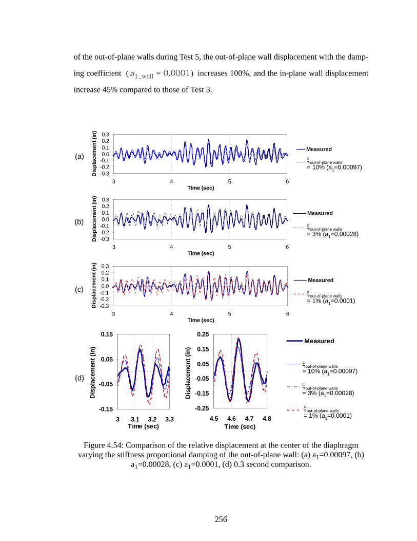
256

of the out-of-plane walls during Test 5, the out-of-plane wall displacement with the damp-

ing coefficient increases 100%, and the in-plane wall displacement

increase 45% compared to those of Test 3.

Figure 4.54: Comparison of the relative displacement at the center of the diaphragm varying the stiffness proportional damping of the out-of-plane wall: (a) a1=0.00097, (b)

a1=0.00028, (c) a1=0.0001, (d) 0.3 second comparison.

a1_wall 0.0001=( )

(a)

(b)

(c)

(d)

-0.3-0.2-0.10.00.10.20.3

3 4 5 6Time (sec)

Dis

plac

emen

t (in

)

Measured

a1 = 0.00097

-0.3-0.2-0.10.00.10.20.3

3 4 5 6Time (sec)

Dis

plac

emen

t (in

)

Measured

a1 = 0.00028

-0.3-0.2-0.10.00.10.20.3

3 4 5 6Time (sec)

Dis

plac

emen

t (in

)

Measured

a1 = 0.00010

-0.15

-0.05

0.05

0.15

3 3.1 3.2 3.3Time (sec)

Dis

plac

emen

t (in

)

-0.25

-0.15

-0.05

0.05

0.15

0.25

4.5 4.6 4.7 4.8Time (sec)

Dis

plac

emen

t (in

)

Measured

a1 = 0.00097

a1 = 0.00028

a1 = 0.00010

ξout-of-plane walls= 10% (a1=0.00097)

ξout-of-plane walls= 3% (a1=0.00028)

ξout-of-plane walls= 1% (a1=0.0001)

ξout-of-plane walls= 10% (a1=0.00097)

ξout-of-plane walls= 3% (a1=0.00028)

ξout-of-plane walls= 1% (a1=0.0001)

257

Figure 4.55: Comparison of the acceleration at the center of the diaphragm varying the stiffness proportional damping of the out-of-plane wall: (a) a1=0.00097, (b) a1=0.00028,

(c) a1=0.0001, (d) 0.3 second comparison.

-3-2-10123

3 4 5 6Time (sec)

Acc

eler

atio

n (g

)

Measured

a1 = 0.00097

-3-2-10123

3 4 5 6Time (sec)

Acc

eler

atio

n (g

)

Measured

a1 = 0.00028

-3-2-10123

3 4 5 6Time (sec)

Acc

eler

atio

n (g

)

Measured

a1 = 0.0001

-3

-2

-1

0

1

2

3

4.5 4.6 4.7 4.8Time (sec)

Acc

eler

atio

n (g

)

Measured

a1 = 0.00097

a1 = 0.00028

a1 = 0.0001

(a)

(b)

(c)

(d)

ξout-of-plane walls= 10% (a1=0.00097)

ξout-of-plane walls= 3% (a1=0.00028)

ξout-of-plane walls= 1% (a1=0.0001)

ξout-of-plane walls= 10% (a1=0.00097)

ξout-of-plane walls= 3% (a1=0.00028)

ξout-of-plane walls= 1% (a1=0.0001)-2

-1.5-1

-0.50

0.51

1.52

3 3.1 3.2 3.3Time (sec)

Acc

eler

atio

n (g

)

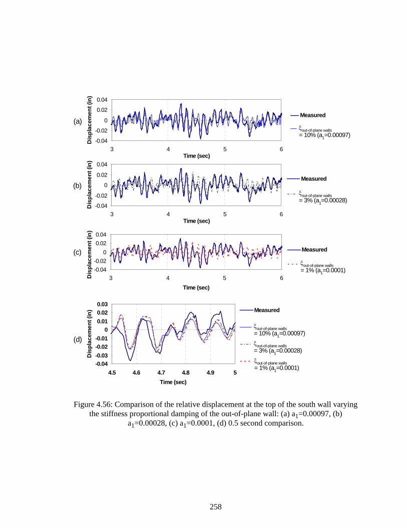
258

Figure 4.56: Comparison of the relative displacement at the top of the south wall varying the stiffness proportional damping of the out-of-plane wall: (a) a1=0.00097, (b)

a1=0.00028, (c) a1=0.0001, (d) 0.5 second comparison.

-0.04

-0.02

0

0.02

0.04

3 4 5 6Time (sec)

Dis

plac

emen

t (in

)

Measured

a1 = 0.00097

-0.04

-0.02

0

0.02

0.04

3 4 5 6Time (sec)

Dis

plac

emen

t (in

)

Measured

a1 = 0.00028

-0.04-0.03-0.02-0.01

00.010.020.03

4.5 4.6 4.7 4.8 4.9 5Time (sec)

Dis

plac

emen

t (in

) Measured

a1 = 0.00097

a1 = 0.00028

a1 = 0.00010

-0.04-0.02

00.020.04

3 4 5 6Time (sec)

Dis

plac

emen

t (in

)

Measured

a1 = 0.00010

(a)

(b)

(c)

(d)

ξout-of-plane walls= 10% (a1=0.00097)

ξout-of-plane walls= 3% (a1=0.00028)

ξout-of-plane walls= 1% (a1=0.0001)

ξout-of-plane walls= 10% (a1=0.00097)ξout-of-plane walls= 3% (a1=0.00028)ξout-of-plane walls= 1% (a1=0.0001)

259

Figure 4.57: Comparison of the acceleration at the top of the south wall varying the stiffness proportional damping of the out-of-plane wall: (a) a1=0.00097, (b) a1=0.00028,

(c) a1=0.0001, (d) 0.2 second comparison.

Figures 4.58 and 4.60 show the comparison of the measured and calculated accel-

eration at the center of the diaphragm. Figures 4.61 and 4.63 show the comparison of the

measured and calculated relative displacement at the center of the diaphragm. The

responses using 10% damping are not plotted here because that they are only slightly dif-

-1.2

-0.6

0

0.6

1.2

3 4 5 6Time (sec)

Acc

eler

atio

n (g

)Measured

a1 = 0.00097

-1.2

-0.6

0

0.6

1.2

3 4 5 6Time (sec)

Acc

eler

atio

n (g

)

Measured

a1 = 0.00028

-1.2

-0.6

0

0.6

1.2

3 4 5 6Time (sec)

Acc

eler

atio

n (g

)

Measured

a1 = 0.00010

-1.5-1

-0.50

0.5

11.5

4.5 4.55 4.6Time (sec)

Acc

eler

atio

n (g

) Measured

a1 = 0.00097

a1 = 0.00028

a1 = 0.00010

(a)

(b)

(c)

(d)

ξout-of-plane walls= 10% (a1=0.00097)

ξout-of-plane walls= 3% (a1=0.00028)

ξout-of-plane walls= 1% (a1=0.0001)

ξout-of-plane walls= 10% (a1=0.00097)

ξout-of-plane walls= 3% (a1=0.00028)ξout-of-plane walls= 1% (a1=0.0001)

260

ferent compared to the responses for 3% damping.

Figure 4.58: Measured acceleration at the center of the diaphragm with PGA =0.67g (Damping: ξdia = 3%, ξwall = 3%).

Figure 4.59: Calculated acceleration at the center of the diaphragm with PGA =0.67g (Damping: ξdia = 3%, ξwall = 3%).

Figure 4.60: Two-second comparison of acceleration at the center of the diaphragm with PGA = 0.67g (Damping: ξdia = 3%, ξwall = 3%).

-3

-2

-1

0

1

2

3

0 1 2 3 4 5 6 7 8 9Time (sec)

Acc

eler

atio

n (g

) Measured

-3

-2

-1

0

1

2

3

0 1 2 3 4 5 6 7 8 9Time (sec)

Acc

eler

atio

n (g

) Calculated

-3

-2

-1

0

1

2

3

4 4.2 4.4 4.6 4.8 5 5.2 5.4 5.6 5.8 6Time (sec)

Acc

eler

atio

n (g

) Measured Calculated

261

Figure 4.61: Comparison of displacement at the center of the diaphragm with PGA = 0.67g (Damping: ξdia = 3%, ξwall = 3%).

Figure 4.62: Comparison of displacement at the center of the diaphragm with PGA = 0.67g (Damping: ξdia = 3%, ξwall = 3%).

Figure 4.63: Two-second comparison of displacement at the center of the diaphragm applying the average acceleration employed in the analysis for PGA = 0 67g (Damping:

ξdia = 3%, ξwall = 3%).

-0.30

-0.20

-0.10

0.00

0.10

0.20

0.30

0 1 2 3 4 5 6 7 8 9

Time (sec)

Dis

plac

emen

t (in

) Measured

-0.30

-0.20

-0.10

0.00

0.10

0.20

0.30

0 1 2 3 4 5 6 7 8 9

T ime (sec)

Dis

plac

emen

t (in

) Calculated

-0.30

-0.20

-0.10

0.00

0.10

0.20

0.30

4 4.2 4.4 4.6 4.8 5 5.2 5.4 5.6 5.8 6Time (sec)

Dis

plac

emen

t (in

) Measured Calculated

262

The peak shear forces at the base of the in-plane and out-of-plane walls are sum-

marized in Table 4.15. The calculated peak in-plane shear force (1.59 kips) of the 3%

damping is higher than the cracking force (1.3 kips) without flange effects shown in Table

4.3. However, the shear force of the 10% damping is similar to the estimated cracking

force. The calculated peak out-of-plane shear force, 2.2 kips shown in Table 4.15, is

higher than the estimated yielding force, 1.42 kips (see Sections 4.3.3.3). The total peak

base shear increases 43% compared to Test 3 (see Table 4.10). The peak shear force of in-

plane walls increases 48% and the shear force of out-of-plane walls increases 36%. As the

damping of in-plane wall increase from 3% to 10%, the peak in-plane shear forces

decrease about 18%.

From the behavior of the out-of-plane and in-plane walls, the following observa-

tion can be made. Due to the damaged out-of-plane walls, the peak relative displacement

of the out-of-plane wall is much larger than that of the in-plane wall in the E-W direction.

The in-plane wall shear forces are increased due to the decreased out-of-plane wall stiff-

ness.

Table 4.15: Calculated shear force at the base using PGA = 0.67 g.

Element

Shear force (lb)

Damping ξdia = 3% ξwall = 3%

Damping ξdia = 3% ξwall=10%

1.South wall 1,590 1,305

2.North wall 1,590 1,305

3.out-of-plane wall (= East + West wall) 2,203 2,290

Total Base Shear (=1+2+3) 5,383 4,900

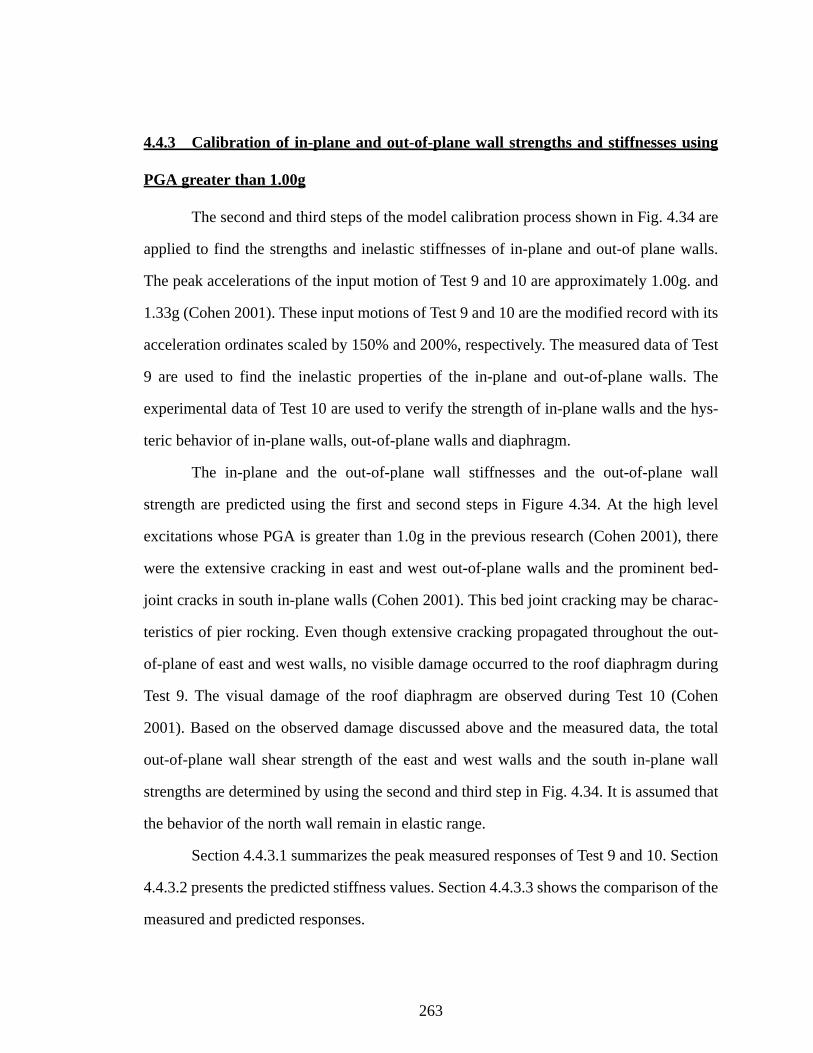
263

4.4.3 Calibration of in-plane and out-of-plane wall strengths and stiffnesses using

PGA greater than 1.00g

The second and third steps of the model calibration process shown in Fig. 4.34 are

applied to find the strengths and inelastic stiffnesses of in-plane and out-of plane walls.

The peak accelerations of the input motion of Test 9 and 10 are approximately 1.00g. and

1.33g (Cohen 2001). These input motions of Test 9 and 10 are the modified record with its

acceleration ordinates scaled by 150% and 200%, respectively. The measured data of Test

9 are used to find the inelastic properties of the in-plane and out-of-plane walls. The

experimental data of Test 10 are used to verify the strength of in-plane walls and the hys-

teric behavior of in-plane walls, out-of-plane walls and diaphragm.

The in-plane and the out-of-plane wall stiffnesses and the out-of-plane wall

strength are predicted using the first and second steps in Figure 4.34. At the high level

excitations whose PGA is greater than 1.0g in the previous research (Cohen 2001), there

were the extensive cracking in east and west out-of-plane walls and the prominent bed-

joint cracks in south in-plane walls (Cohen 2001). This bed joint cracking may be charac-

teristics of pier rocking. Even though extensive cracking propagated throughout the out-

of-plane of east and west walls, no visible damage occurred to the roof diaphragm during

Test 9. The visual damage of the roof diaphragm are observed during Test 10 (Cohen

2001). Based on the observed damage discussed above and the measured data, the total

out-of-plane wall shear strength of the east and west walls and the south in-plane wall

strengths are determined by using the second and third step in Fig. 4.34. It is assumed that

the behavior of the north wall remain in elastic range.

Section 4.4.3.1 summarizes the peak measured responses of Test 9 and 10. Section

4.4.3.2 presents the predicted stiffness values. Section 4.4.3.3 shows the comparison of the

measured and predicted responses.

264

4.4.3.1 Measured responses

Tables 4.16 and 4.17 summarizes the peak measured responses of Tests 9 and 10,

respectively, corresponding to the locations shown in Fig. 4.4. The complete measured

time history responses are plotted in Figs. C.31 through C.44 in Appendix C. The peak

acceleration and displacement at the center of the diaphragm are 3.28 g and 0.46 in,

respectively for Test 9. The test shows slight different peak acceleration between the north

(1.26g) and south wall (1.37g). The difference may be attributed to experimental errors in

the lifting frame, as discussed in Section 4.3.4. The measured peak relative displacements

at the top of north and south walls are 0.053 in (see Table 4.16). The peak relative dis-

placement, 0.92 in (Test 10) at the center of the diaphragm is higher than 0.46 in (Test9)

(see Tables 4.16 and 4.17). It is due to the extensive damage of the out-of-plane walls.

Table 4.16: Summary of measured accelerations and displacements in the E-W direction (PGA = 1.0g).

LocationPeak Acceleration (g) Peak displacement (in)

Instrument Test 9 Instrument Test 9

South wallA104a 1.3105

D104 0.053A104b 1.3736

Diaphragm A105 3.2862 D105 0.457

North wallA106a 1.2585

D106 0.053A106b 1.2555

265

Table 4.17: Summary of measured accelerations and displacements in the E-W direction (PGA = 1.33g).

4.4.3.2 Summary of predicted properties

The predicted properties are summarized in Table 4.18. The initial stiffnesses of

the in-plane and out-of-plane walls are obtained from Tests 3 and 5, (see Tables 4.8 and

4.13). For the nonlinear time history analyses, the rocking model discussed in Section

4.3.2 is applied to the in-plane and out-of-plane wall elements and the three parameter

model is applied to the diaphragm element (see Sections 4.3.2 and 4.3.3). The in-plane

wall damping ratio of 10% is used to obtain the predicted values

By comparing the overall history of the measured and calculated responses, the in-

plane wall strength and out-of-plane stiffnesses and strength are calibrated. The estimated

in-plane stiffness and strength of south wall are 50 kips/in and 1.75 kips, respectively. The

predicted strength, 1.75 kips is higher than the estimated cracking strength, 1.3 kips, but

smaller than the yield strength, 2.26 kips (see Section 4.3.3). The out-of-plane strength

and inelastic stiffness are reduced to 0.4 kips and 2 kips/in compared to the previous pre-

dicted properties, 0.6 kips and 9 kips/in (see Table 4.13). This is due to the accumulated

damage in the out-of-plane walls during Tests 6 to 7, which are done between Test 5 and 9.

LocationPeak Acceleration (g) Peak displacement (in)

Instrument Test 10 Instrument Test 10

South wallA104a 1.768

D104 0.076A104b 1.801

Diaphragm A105 4.810 D105 0.921

North wallA106a 1.547

D106 0.072A106b 1.222

266

Table 4.18: Predicted properties from the calibration process (PGA=1.0g).

The comparison of the analyses using two different damping ratios shows that the

nonlinear responses of the building are sensitive to this variable. Because 3% damping

corresponds to essentially elastic response, the effective damping should be increased

when hysteretic behavior occurs. Two different damping ratios (3% and 10%) are used to

investigate the effect of the damping ratio within the masonry walls. The sensitivity of the

damping ratio is now discussed.

Effects of masonry wall damping ratios

A frequency analysis is performed to find the Rayleigh damping coefficients using

the predicted properties (see Table 4.18). Due to the decreased out-of-plane wall stiffness,

the frequencies of the first and third modes (65 and 140 rad/sec, respectively) are

changed. The Rayleigh damping coefficients and of the lumped

masses at the common DOFs (X in Fig. 4.28) are 2.67. The Rayleigh damping coefficients

of the diaphragm is 0.00029 for a damping ratio of 3%

Figure 4.64 shows the comparison of the time history responses varying the in-

plane wall damping ratios. When a damping ratio of 3% is used

for the in-plane walls, the time history response shows the unstable curves between 4.4

and 4.7 sec shown in Figs. 4.64 (c) and (d). When a damping ratio of 5%

Component Stiffness Strength

In-plane Walls 50 kips/in 1.75 kips

Out-of-plane Wall K1 = 11 kips/in, K2 = 2 kips/in

(=East + West Wall)

0.4kips

Equivalent dia-phragm stiffness

(Get)1

8.82 kips/in (see Section 4.3.2.2)F1 = 0.1 ksi, F2 = 0.69 ksi

a0_wall a0_diaphragm

a1_diaphragm

a1_wall 0.00029=( )

267

is used for the in-plane walls, the peak response is reduced but is

unstable compared to the measured history responses. The time history response with 10%

damping for the in-plane walls fit well with the measured response

(see Figs. 4.64 (a) and (d)). It appears that the 3% damping ratio obtained from the sine-

decay tests (see Section 4.3.6) can be applied to the diaphragm element and can not be

applied to the in-plane walls for the non-linear time history analysis. The 10% damping

ratio of the in-plane walls is an appropriate choice to give results comparable to the

observed response of the physical structure. However, the responses of the diaphragm are

not changed due to the changes in the damping ratios of the in-plane walls, as shown in

Fig. 4.65.

a1_wall 0.00049=( )

a1_wall 0.00098=( )

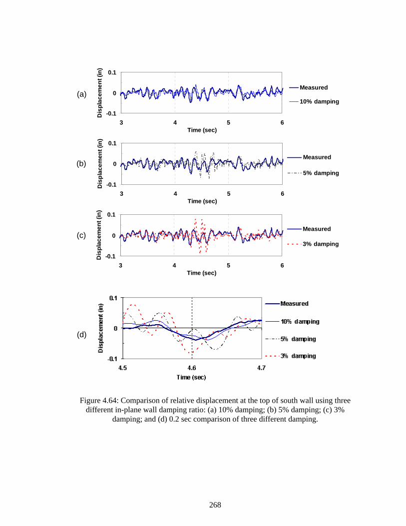
268

Figure 4.64: Comparison of relative displacement at the top of south wall using three different in-plane wall damping ratio: (a) 10% damping; (b) 5% damping; (c) 3%

damping; and (d) 0.2 sec comparison of three different damping.

-0.1

0

0.1

3 4 5 6Time (sec)

Dis

plac

emen

t (in

)

Measured

10% damping

-0.1

0

0.1

3 4 5 6Time (sec)

Dis

plac

emen

t (in

)

Measured

5% damping

-0.1

0

0.1

3 4 5 6Time (sec)

Dis

plac

emen

t (in

)

Measured

3% damping

(a)

(b)

(c)

(d)

269

Figure 4.65: Comparison of relative displacement at the center of diaphragm using three different in-plane wall damping ratio: (a) 10% damping; (b) 5% damping; (c) 3%

damping; and (d) 0.2 sec comparison of three different damping.

In summary, the above studies as well as the studies discussed in Sections 4.4.1.3

and 4.4.2.3 indicate that the following damping assumptions provide good correlation

(a)

(b)

(c)

(d)

-0.6-0.3

00.3

0.6

3 4 5 6Time (sec)

Dis

plac

emen

t (in

)

Measured

5% damping

-0.6-0.3

0

0.30.6

3 4 5 6Time (sec)

Dis

plac

emen

t (in

)

Measured

10% damping

-0.6

-0.30

0.3

0.6

3 4 5 6Time (sec)

Dis

plac

emen

t (in

)

Measured

3% damping

270

with all of the results from tests 3, 5 and 9:

• 3% damping for the diaphragms and for the out-of-plane walls. This leads to damping coefficients of = 2.932, =0.000278 , =2.932 and

= 0.000278.

• 10 % damping for the in-plane walls. This leads to damping coefficients of

= 2.932 and = 0.00097.

In-plane wall strength

The rocking hysteresis model developed in this research is used for the masonry

walls. The predicted hysteretic curve of south wall is shown in Fig. 4.66. The in-plane

north wall is assumed to be elastic based on the observed damage, as shown in Fig. 4.67.

The properties of south wall are determined by decreasing shear strength as shown in Fig.

4.68. When the in-plane strength of south wall is reduced from infinite (elastic) to 2.0

kips, the peak relative displacements of the south wall, 0.043 in, are not changed. Because

the nonlinear action of the south wall is not significant, it does not affect the response of

the building. When the in-plane strength of south wall reduced to 1.75 kips, the peak rela-

tive displacement increases to 0.051in compared to the measured value of 0.053 in.

a0_diaphragm a1_diaphragm a0_wall

a1_wall

a0_wall

a1_wall

271

Figure 4.66: In-plane south wall hysteresis curve employed in the analysis for PGA = 1.0g (Damping: ξdia = 3%, ξwall = 10%).

Figure 4.67: In-plane north wall hysteresis curve employed in the analysis for PGA = 1 0g (Damping: ξdia = 3%, ξwall = 10%).

-2

-1

0

1

2

-0.1 0 0.1

In-plane Drift Ratio (%)

In-p

lane

Wal

l She

ar F

orce

(k

ips)

-3

-2

-1

0

1

2

3

-0.1 0 0.1

In-plane Drift Ratio (% )

In-p

lane

Wal

l She

ar F

orce

(k

ips)

272

Figure 4.68: Comparison of force and displacement at the south wall using three different in-plane wall strength: (a) Fy = infinite; (b) Fy = 2.0 kips; (c) Fy = 1.75 kips; and (d) 0.2

sec comparison of three different strength. (Damping: ξdia = 3%, ξwall = 10%).

(a)

(b)

(c)

(d)

-0.06

0

0.06

3 4 5 6Time (sec)

Dis

plac

emen

t (in

) Measured Fy = infinite

-0.06

0

0.06

3 4 5 6Time (sec)

Dis

plac

emen

t (in

) Measured Fy = 2.0 kips

-0.06

0

0.06

3 4 5 6Time (sec)

Dis

plac

emen

t (in

) Measured Fy= 1.75 kips

-2.5

0

2.5

-0.07 0 0.07

In-plane Drift Ratio (%)

In-p

lane

Wal

l She

ar

Forc

e (k

ips)

-2.5

0

2.5

-0.07 0 0.07

In-plane Drift Ratio (%)

In-p

lane

Wal

l She

ar

Forc

e (k

ips)

-2.5

0

2.5

-0.07 0 0.07

In-plane Drift Ratio (%)

In-p

lane

Wal

l She

ar

Forc

e (k

ips)

273

Out-of-plane wall strength and stiffness

The predicted initial and second tangent stiffness of out-of-plane wall are

decreased to 11 and 2 kips/in, respectively, because the accumulated damage of the out-of-

plane walls during the previous tests (Tests 6, 7, and 8) (see Table 4.13). The predicted

strength of the out-of-plane wall also decreases 0.4 kips compared to the shear strength of

0.6 kips in Table 4.13. The hysteretic behavior of the out-of-plane east and west walls is

shown in Fig. 4.69. As the in-plane and out-of-plane walls are damaged, the visible inelas-

tic behavior of diaphragm can occur during Test 9, as shown in Fig. 4.70. Time history

responses are compared in Section 4.4.3.3.

Figure 4.69: Out-of-plane wall hysteresis curve employed in the analysis for PGA = 1 0g (Damping: ξdia = 3%, ξwall = 10%).

-1.4

-0.7

0

0.7

1.4

-0.6 -0.3 0 0.3 0.6

Out-of-plane Drift Ratio (% )

Out

-of-p

lane

Wal

l She

ar F

orce

(k

ips)

274

Figure 4.70: Diaphragm Hysteresis curve employed in the analysis for PGA = 1.0g (Damping: ξdia = 3%, ξwall = 10%).

4.4.3.3 Comparison between measured and calculated response

Table 4.19 summarizes the comparison of the measured and calculated peak

responses of the structure using the damping ratio of 10% for the masonry walls and the

damping ratio of 3% for the diaphragm. The non-linear analysis uses the predicted proper-

ties shown in Table 4.18.

-1.2

-0.6

0

0.6

1.2

-0.3 -0.2 -0.1 0 0.1 0.2 0.3

Diaphragm Drift Ratio (%)

Dia

phra

gm S

hear

For

ce (k

ips)

275

Table 4.19: Comparison of measured and calculated response using PGA = 1.0 g ( ξdia = 3%, ξwall = 10%).

The peak relative displacement at the top of the south wall is 0.051 in compared to

the measured one, 0.053in. The calculated and measure drift ratios of the in-plane south

wall is 0.06%. The drift ratio is much lower than the drift limitation (0.4%) of the immedi-

ate occupancy level in FEMA 356 (see Table 4.20). However, there is significant bed-joint

cracking along the bottom of the south in-plane wall. The comparison of the calculated

and measured displacement time history responses is shown in Figs. 4.71 and 4.73. The

peak acceleration at the top of the south wall (1.38 g) is compared with the measured one

(1.37g) (see Figs. 4.74 and 4.76). The calculated acceleration and displacement at the top

of south wall are matched well with the measured ones. The calculated peak acceleration

at the top of the north wall (1.39g) is slightly higher than the measured one (1.26g).

The calculated relative displacement at the center of the diaphragm is 0.41 in com-

pared to the measured value of 0.45 in. The drift ratios of the out-of-plane wall associated

with the diaphragm displacement is 0.54%. The drift ratio is much lower than the drift

limitation (2%) of the immediate occupancy level in FEMA 356 (see Table 4.20). How-

ever, the building shows extensive cracking. Figures 4.77 to 4.79 show the comparison of

displacement at the center of the diaphragm. The initial time range (from 3 to 4 sec) shows

Compared Item Measured Calculated (MDOF model)

Center of diaphragm (105)Acceleration 3.28 g 2.10 g

Displacement 0.45 in 0.41 in

North wall (106)Acceleration 1.32 g 1.39 g

Displacement 0.053 in 0.043 in

South wall (104)Acceleration 1.37 g 1.38 g

Displacement 0.053 in 0.051 in

276

that the predicted structural property seems to be overestimated. As the stiffness of the

diaphragm is degraded after 4 seconds, the overall displacement time history responses are

matched well with measured response, as shown in Fig. 4.79 However, the peak accelera-

tion at the center of the diaphragm (2.01 g) is less than the measured acceleration (3.28 g).

Figures 4.80 to 4.82 show the comparison of acceleration at the center of the diaphragm.

Table 4.20: Structural performance criteria for RM structure in FEMA356 (ASCE 2002a).

The relative displacement is captured at the top of the west wall and the accelera-

tion is measured at the center of the diagonally sheathed diaphragm, as shown in Figs. 4.3

and 4.4. At strong excitation (PGA > 1.0g), damage of the diaphragm were observed

(Cohen 2001). This nonlinear behavior of the diagonally sheathed diaphragm shown in

Fig. 4.3 may cause the discrepancy between the measured and calculated acceleration,

because the acceleration instrument was located on the diagonal sheathing, as shown in

Figs. 4.3 and 4.4. When the peak input ground motion of 1.33 g (Test 10) is applied to this

building, the problem is significant. The calculated acceleration of Test 10 is 2.6g com-

Masonry Element Immediate Occupancy Life Safety Collapse

Prevention

Reinforced

(7.4.5.3 in FEMA356)

In-plane wall(Controlled by

shear)

0.4% 0.6% 0.75%

Out-of-plane wall 2% 3% 5%

Reinforced Masonry walls (Table C1-3 in FEMA 356) 0.2% 0.6% 1.5%

Damage states Minor crack-ing

Extensive cracking Crushing

277

pared to the measured one, 4.8g. The comparison of these accelerations is shown in Figs.

4.83 to 4.85.

Figure 4.71: Measured displacement at the top of south wall with PGA = 1.0g (Damping: ξdia = 3%, ξwall = 10%).

Figure 4.72: Calculated displacement at the top of south wall with PGA = 1.0g (Damping: ξdia = 3%, ξwall = 10%).

Figure 4.73: Two-second comparison of displacement at the top of south wall with PGA =1.0g (Damping: ξdia = 3%, ξwall = 10%).

-0.06-0.04-0.020.000.020.040.06

0 1 2 3 4 5 6 7 8 9Time (sec)

Dis

plac

emen

t (in

)

-0.06-0.04-0.020.000.020.040.06

0 1 2 3 4 5 6 7 8 9Time (sec)

Dis

plac

emen

t (in

)

-0.06-0.04-0.020.000.020.040.06

3.5 4 4.5 5 5.5Time (sec)

Dis

plac

emen

t (in

) Measured Calculated

278

Figure 4.74: Measured acceleration at the top of south wall with PGA = 1.0g (Damping: ξdia = 3%, ξwall = 10%).

Figure 4.75: Calculated acceleration at the top of south wall with PGA = 1.0g (Damping: ξdia = 3%, ξwall = 10%).

Figure 4.76: Two-second comparison of acceleration at the top of south wall with PGA =1.0g (Damping: ξdia = 3%, ξwall = 10%).

-1.50-1.00-0.500.000.501.001.50

0 1 2 3 4 5 6 7 8 9Time (sec)

Acc

eler

atio

n (g

)

-2.00-1.50-1.00-0.500.000.501.001.50

0 1 2 3 4 5 6 7 8 9Time (sec)

Acc

eler

atio

n (g

)

-2.00-1.50-1.00-0.500.000.501.001.50

3.5 4 4.5 5 5.5Time (sec)

Acc

eler

atio

n (g

)

Measured Calculated

279

Figure 4.77: Measured displacement at the center of the diaphragm with PGA = 1.0g (Damping: ξdia = 3%, ξwall = 10%).

Figure 4.78: Calculated displacement at the center of the diaphragm with PGA = 1.0g (Damping: ξdia = 3%, ξwall = 10%).

Figure 4.79: Two-second comparison of displacement at the center of the diaphragm with PGA = 1.0g (Damping: ξdia = 3%, ξwall = 10%).

-0.6

-0.4

-0.2

0.0

0.2

0.4

0.6

0 1 2 3 4 5 6 7 8 9 10Time (sec)

Dis

plac

emen

t (in

) Measured

-0.5-0.4-0.3-0.2-0.10.00.10.20.30.40.5

0 1 2 3 4 5 6 7 8 9 10T ime (sec)

Dis

plac

emen

t (in

) Calculated

-0.6

-0.4

-0.2

0

0.2

0.4

0.6

4.5 4.7 4.9 5.1 5.3 5.5 5.7 5.9 6.1 6.3 6.5Time (sec)

Dis

plac

emen

t (in

)

Measured Calculated

280

Figure 4.80: Measured acceleration at the center of the diaphragm with PGA = 1.0g (Damping: ξdia = 3%, ξwall = 10%).

Figure 4.81: Calculated acceleration at the center of the diaphragm with PGA = 1.0g (Damping: ξdia = 3%, ξwall = 10%).

Figure 4.82: Two-second comparison of acceleration at the center of the diaphragm with PGA = 1.0g (Damping: ξdia = 3%, ξwall = 10%).

-4-3

-2-101

23

0 1 2 3 4 5 6 7 8 9Time (sec)

Acc

eler

atio

n (g

)Measured

-3

-2

-1

0

1

2

3

0 1 2 3 4 5 6 7 8 9Time (sec)

Acc

eler

atio

n (g

)

Calculated

-4-3-2-10123

4.5 4.7 4.9 5.1 5.3 5.5 5.7 5.9 6.1 6.3 6.5Time (sec)

Acc

eler

atio

n (g

)

Measured Calculated

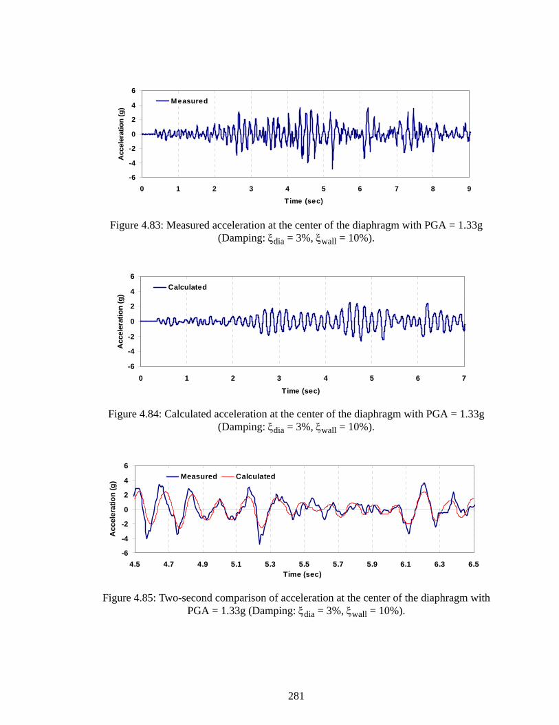
281

Figure 4.83: Measured acceleration at the center of the diaphragm with PGA = 1.33g (Damping: ξdia = 3%, ξwall = 10%).

Figure 4.84: Calculated acceleration at the center of the diaphragm with PGA = 1.33g (Damping: ξdia = 3%, ξwall = 10%).

Figure 4.85: Two-second comparison of acceleration at the center of the diaphragm with PGA = 1.33g (Damping: ξdia = 3%, ξwall = 10%).

-6

-4

-2

0

2

4

6

0 1 2 3 4 5 6 7 8 9T ime (sec)

Acc

eler

atio

n (g

)

Measured

-6

-4

-2

0

2

4

6

0 1 2 3 4 5 6 7

Time (sec)

Acc

eler

atio

n (g

)

Calculated

-6

-4

-2

0

2

4

6

4.5 4.7 4.9 5.1 5.3 5.5 5.7 5.9 6.1 6.3 6.5Time (sec)

Acc

eler

atio

n (g

) Measured Calculated

282

The calculated shear forces at the base are summarized in Table 4.21. The total

base shear increases 66% compared to Test 3 as shown in Table 4.10. The shear force of

in-plane walls increases 138%, but the shear force of out-of-plane walls decrease 29%.

Due to the extensive damage of the out-of-plane wall, the increased lateral force of the

structure is much more distributed to the in-plane walls than to the damaged out-of-plane

walls.

Table 4.21: Calculated seismic shear at the base using PGA = 1.0 g (Damping ξdia = 3% ξwall= 10%).

4.5 Sensitivity Analysis

In this section, parametric sensitivity analyses are performed using the structural

properties obtained from the model calibration process as base reference values. In these

analyses, the stiffness and strength of the backbone curves for the diaphragm, the out-of-

plane walls, and the in-plane walls are varied as illustrated in Figs. 4.86 and 4.88. Figure

4.86 shows the backbone curves for a number of the analyses that span the complete range

of parameters considered. The hysteresis properties of the varied curves are unchanged

from those selected by the calibration procedure. The model maxima are computed using

Element Shear Force(lb.)

1. North wall 1,797 lb.

2. South wall 2,125 lb.

3. out-of-plane wall (= East + West wall) 1,147 lb.

4. East wall 165 lb.

5. West wall 156 lb.

Overall Base Shear (=1+2+3) 5,069 lb.

283

the nonlinear time history analysis with two different ground accelerations (PGA = 0.5g

and 1.0g) obtained from Tests 3 and 9. The main objective is to capture the nonlinear

dynamic characteristics of the building under the moderate and strong earthquakes. The

analytical results in these figures are normalized to the predicted element properties

obtained from the model calibration process. In each figure, the normalized parameter ver-

sus the out-of-plane and in-plane drift ratios in percent is plotted. Each of the figures

focuses on illustrating the effects on the out-of-plane and in-plane wall drift. The mass

properties are assumed to be the same in all the models of the sensitivity study for pur-

poses of simplicity. In these sensitivity analyses, 3% damping is applied to diaphragm and

10% damping is applied to the masonry walls (see Section 4.4.3.2).

4.5.1 Effect of diaphragm flexibility

The diaphragm stiffness (Kd) is normalized by the obtained diaphragm stiffness

from the quasi static test results (Kd*) (see Section 4.3.2.2). The normalized diaphragm

stiffness (Kd/Kd*) is used to plot the backbone curves of the diaphragm. The normalized

diaphragm stiffness (Kd/Kd*) is plotted against the out-of-plane and in-plane drift ratios in

percent. Figures 4.89 through 4.94 summarize the displacement and acceleration results

from all the sensitivity studies varying diaphragm flexibility. The following trends can be

observed from the plots.

• For both 0.5g and 1.0g input ground motions, as the diaphragm stiffness is

increased from Kd/Kd* = 1 to 5, the out-of-plane wall drift ratio is decreased, as

shown in Figs. 4.89 and 4.90, but the in-plane wall drift ratio is increased, as

shown in Fig. 4.92.

• For 0.5 g input ground motion, the overall response of the building is elastic

between Kd/Kd* = 3 to rigid diaphragm. As the diaphragm goes from Kd/Kd* =

3 to very flexible diaphragm, the behavior of out-of-plane walls becomes

inelastic. As the diaphragm goes from Kd/Kd* = 3 to 1, the in-plane wall drift

284

ratios are slightly increased. As the diaphragm goes from Kd/Kd* = 1 to very

flexible diaphragm, the in-plane wall drift ratios are not changed as rapidly as

the out-of-plane wall drift ratio. As the diaphragm goes from Kd/Kd* = 0.7 to 2

(see Fig. 4.90), the in-plane and out-of-plane wall drift ratios are increased

compared to the results of Kd/Kd* = 2.9.

• For 1.0g input ground motion, as the diaphragm stiffness ratio (Kd/Kd*) is

increased from 0.4 to 2.9, the out-of-plane drift ratio is gradually decreased

(see Fig. 4.90), but the in-plane wall drift is increased above the immediate

occupancy level in FEMA356, as shown in Figs. 4.91 and 4.92 (a). However,

as the diaphragm stiffness ratio is increased from 3, the in-plane wall drift ratio

is decreased, but after passing 25, the drift ratio remains about 0.11%. From the

point where diaphragm stiffness ratio equals 6 to rigid diaphragm, the behavior

of the diaphragm is elastic (see Fig. 4.92(d)). The behavior of the diaphragm is

inelastic for diaphragm stiffness ratios between 0.4 and 3. The out-of-plane and

in-plane wall are in inelastic range on the whole. The in-plane drift ratio has a

maximum value at a stiffness ratio of 3. The peak in-plane drift ratio of 3 can

be treated as the similar phenomenon, as shown in the SDOF spectral response

in Fig. 4.95. Spectral displacement value is maximized around 0.1sec. The cal-

culated natural period of the test building is 0.08sec (Table 4.9). As the stiff-

ness of out-of-plane and in-plane walls are degraded, the period of the structure

will be increased around 0.10 sec. In addition, if the assumed stiffness propor-

tional damping for non-linear analysis is increased, the corresponding maxi-

mum value where stiffness ratio is 3 will be decreased in the analytical model.

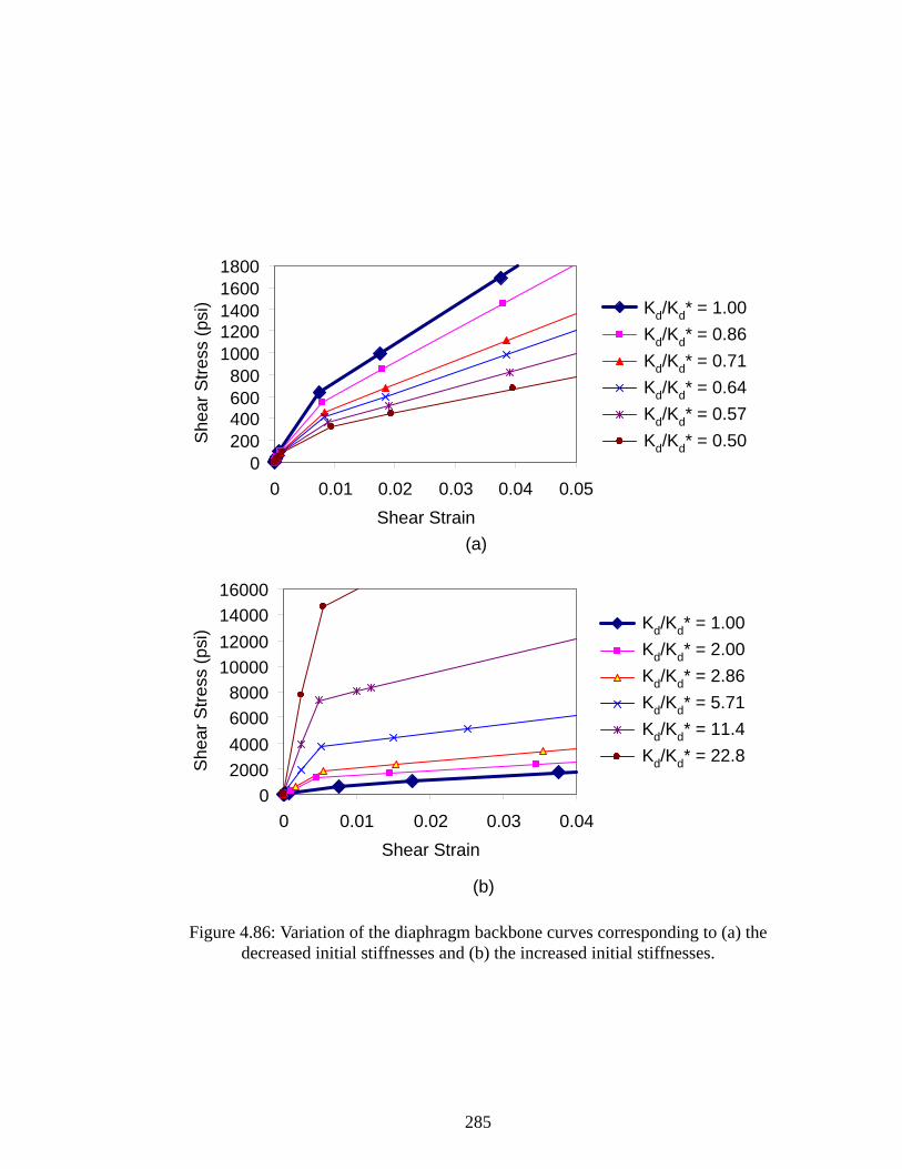
285

Figure 4.86: Variation of the diaphragm backbone curves corresponding to (a) the decreased initial stiffnesses and (b) the increased initial stiffnesses.

02000400060008000

10000120001400016000

0 0.01 0.02 0.03 0.04Shear Strain

She

ar S

tress

(psi

) Ge = 140000Ge = 200000Ge = 400000Ge = 800000Ge = 1600000Ge = 3200000

0200400600800

10001200140016001800

0 0.01 0.02 0.03 0.04 0.05Shear Strain

She

ar S

tress

(psi

) Ge = 140000Ge=120000Ge=100000Ge=90000Ge=80000Ge=70000

Kd/Kd* = 1.00Kd/Kd* = 0.86Kd/Kd* = 0.71Kd/Kd* = 0.64Kd/Kd* = 0.57Kd/Kd* = 0.50

Kd/Kd* = 1.00Kd/Kd* = 2.00Kd/Kd* = 2.86Kd/Kd* = 5.71Kd/Kd* = 11.4Kd/Kd* = 22.8

(a)

(b)

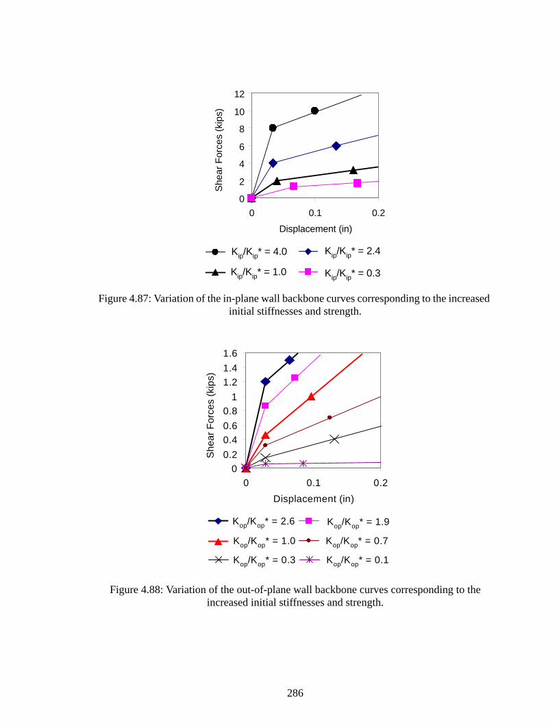
286

Figure 4.87: Variation of the in-plane wall backbone curves corresponding to the increased initial stiffnesses and strength.

Figure 4.88: Variation of the out-of-plane wall backbone curves corresponding to the increased initial stiffnesses and strength.

0

2

4

6

8

10

12

0 0.1 0.2

Displacement (in)S

hear

For

ces

(kip

s)

Kip/Kip* = 4.0 Kip/Kip* = 2.4

Kip/Kip* = 1.0 Kip/Kip* = 0.3

00.20.40.60.8

11.21.41.6

0 0.1 0.2Displacement (in)

She

ar F

orce

s (k

ips)

Kop/Kop* = 2.6 Kop/Kop* = 1.9

Kop/Kop* = 0.1Kop/Kop* = 0.3

Kop/Kop* = 1.0 Kop/Kop* = 0.7

287

Figure 4.89: Peak out-of-plane wall drift ratio varying the diaphragm stiffness from Kd/Kd* = 0.4 (flexible diaphragm) to 40 (rigid diaphragm).

0.0

0.1

0.2

0.3

0.4

0.5

0.6

0.7

0.8

0.9

0 10 20 30 40Normalized Diaphragm Stiffness

( Kd / Kd* )

Peak

Out

-of-p

lane

Wal

l Drif

t Rat

io (%

)

PGA=0.5g

PGA=1.0g

288

Figure 4.90: (a) Peak out-of-plane wall drift ratio varying the diaphragm stiffness from Kd/Kd* = 0.4 (very flexible diaphragm) to 5 (flexible diaphragm), (b) Hysteretic curves of

structural components for Kd/Kd* = 0.7; (c) for Kd/Kd* = 2; and (d) for Kd/Kd* = 2.9.

0.0

0.1

0.2

0.3

0.4

0.5

0.6

0.7

0.8

0 1 2 3 4 5Normalized Diaphragm Stiffness

( Kd / Kd* )

Peak

Out

-of-p

lane

Wal

l Drif

t Rat

io (%

)

PGA=0.5g

PGA=1.0g

Out-of-plane wall

-1

0

1

-0.2 0.3

Displacement (in)

Shea

r For

ce (k

ips)

Diaphragm

-0.4

0

0.4

-0.002 0 0.002

Shear Strain

She

ar S

tress

(ksi

)

Out-of-plane wall

-1

0

1

-0.2 0 0.2

Displacement (in)

She

ar F

orce

(k

ips)

Diaphragm

-0.4

0

0.4

-0.002 0 0.002

Shear Strain

She

ar S

tress

(k

si)

Diaphragm

-0.4

0

0.4

-0.002 0 0.002

Shear Strain

Shea

r Stre

ss

(ksi

)

Out-of-plane wall

-1

0

1

-0.2 0.0 0.2

Displacement (in)

Shea

r For

ce (k

ips)

In-plane wall

-2

-1

0

1

2

-0.04 0.00 0.04

Displacement (in)

Shea

r For

ce (k

ips)

In-plane wall

-2

-1

0

1

2

-0.04 0.00 0.04

Displacement (in)

Shea

r For

ce (k

ips)

In-plane wall

-2

0

2

-0.04 0.00 0.04

Displacement (in)

Shea

r For

ce (k

ips)

(a)

(b) (c) (d)

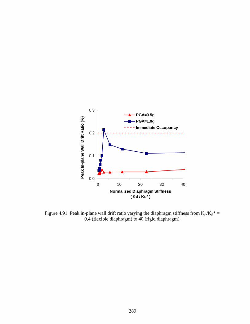
289

Figure 4.91: Peak in-plane wall drift ratio varying the diaphragm stiffness from Kd/Kd* = 0.4 (flexible diaphragm) to 40 (rigid diaphragm).

0.0

0.1

0.2

0.3

0 10 20 30 40

Normalized Diaphragm Stiffness ( Kd / Kd* )

Peak

In-p

lane

Wal

l Drif

t Rat

io (%

) PGA=0.5gPGA=1.0gImmediate Occupancy

290

Figure 4.92: (a) Peak in-plane wall drift ratio varying the diaphragm stiffness from Kd/Kd* = 0.4 (very flexible diaphragm) to 6 (flexible diaphragm) (b) Hysteretic curves of

structural components for Kd/Kd* = 2; (c) for Kd/Kd* = 2.9; and (d) for Kd/Kd* = 5.7.

0.0

0.1

0.2

0 1 2 3 4 5 6Normalized Diaphragm Stiffness

( Kd / Kd*)

Peak

In-p

lane

Wal

l Drif

t Rat

io (%

)

PGA=0.5g

PGA=1.0g

ImmediateOccupancy

Out-of-plane wall

-1

0

1

-0.4 0.0 0.4

Displacement (in)

She

ar F

orce

(k

ips)

Diaphragm

-0.6

0

0.6

-0.003 0 0.003

Shear Strain

Shea

r Stre

ss

(ksi

)

In-plane wall

-3-2-10123

-0.1 0.0 0.1

Displacement (in)

She

ar F

orce

(k

ips)

Out-of-plane wall

-1

0

1

-0.4 0.0 0.4

Displacement (in)

Shea

r For

ce (k

ips)

Diaphragm

-0.6

0

0.6

-0.003 0 0.003

Shear Strain

Shea

r Stre

ss

(ksi

)

In-plane wall

-3-2-10123

-0.2 0.0 0.2

Displacement (in)

She

ar F

orce

(k

ips)

Out-of-plane wall

-1

0

1

-0.4 0.0 0.4

Displacement (in)S

hear

For

ce

(kip

s)Diaphragm

-0.6

0.0

0.6

-0.003 0.000 0.003

Shear Strain

Shea

r Stre

ss

(ksi

)

In-plane wall

-3-2-10123

-0.2 0.0 0.2

Displacement (in)

She

ar F

orce

(k

ips)

(a)

(b) (c) (d)

291

Figure 4.93: Peak acceleration at diaphragm varying the diaphragm stiffness from Kd/Kd* = 0.4 (flexible diaphragm) to 40 (rigid diaphragm).

Figure 4.94: Peak acceleration at diaphragm varying the diaphragm stiffness from Kd/Kd* = 0.4 (very flexible diaphragm) to 5 (flexible diaphragm).

0.0

0.5

1.0

1.5

2.0

2.5

3.0

3.5

0 10 20 30 40

Normalized Diaphragm Stiffness ( Kd / Kd* )

Peak

Acc

eler

atio

n at

Dia

phra

gm (g

)

PGA=0.5g

PGA=1.0g

0.0

0.5

1.0

1.5

2.0

2.5

3.0

3.5

0 1 2 3 4 5

Normalized Diaphragm Stiffness ( Kd / Kd*)

Peak

Acc

eler

atio

n at

Dia

phra

gm (g

) PGA=0.5g

PGA=1.0g

292

Figure 4.95: Displacement response spectrum of time-scaled (factor = 0.5) input record used for ground excitation.

4.5.2 Effect of in-plane wall stiffness and strength

Figures 4.96 through 4.98 summarize the displacement and acceleration results

from all the sensitivity studies varying in-plane wall stiffness. The normalized in-plane

wall stiffness ratio (Kip/Kip*) is plotted against the out-of-plane, in-plane drift ratios in

percents. Kip* is the in-plane wall stiffness obtained from the model calibration process

(see Table 4.18). The following characteristics can be observed from the plots in Figs.

4.96 through 4.98.

• For both 0.5 g and 1.0g input ground motion, as the in-plane wall stiffness ratio

is increased from 0.33 to 4, both the out-of-plane and in-plane wall drift ratios

are decreased.

• For 0.5g input ground motion, the out-of-plane wall drift ratios, as shown in Fig.

4.96, are not significantly influenced by changing the in-plane wall stiffness

ratio from 0.5 to 4.

0.0

0.2

0.4

0.6

0.8

0.05 0.1 0.15Period (sec)

Spec

tral D

ispl

acem

ent (

in)

PGA=0.5g, 3%PGA=0.5g, 5%PGA=1.0g, 3%PGA=1.0g, 5%

293

Figure 4.96: Peak out-of-plane wall drift ratio varying the in-plane wall stiffness from Kip/Kip* = 0.33 to 4.

Figure 4.97: Peak in-plane wall drift ratio varying the in-plane wall stiffness from Kip/Kip* = 0.33 to 4.

0.00

0.20

0.40

0.60

0.80

0 1 2 3 4

Normalized In-plane Wall Stiffness (Kip / Kip*)

Peak

Out

-of-p

lane

Wal

l Drif

t Rat

io (%

) PGA=0.5g

PGA=1.0g

0.00

0.02

0.04

0.06

0.08

0.10

0.12

0.14

0.16

0.18

0 1 2 3 4

Normalized In-plane Wall Stiffness (Kip / Kip*)

Peak

In-p

lane

Wal

l Drif

t Rat

io (%

) PGA=0.5g

PGA=1.0g

294

Figure 4.98: Peak acceleration at diaphragm varying the in-plane wall stiffness from Kip/Kip* = 0.33 to 4.

4.5.3 Effect of out-of-plane wall stiffness and strength

Figures 4.99 through 4.101 summarize the peak displacement and acceleration

results from all the sensitivity results varying out-of-plane wall stiffness. The normalized

out-of-plane wall stiffness ratio (Kop/Kop*) is plotted versus the out-of-plane, in-plane

drift ratios in percents. Kop* is the out-of-plane wall stiffness obtained from the model

calibration process (see Table 4.18). The following trends can be observed from the plots

in Figure 34 and 35.

• For 0.5g input ground motion, as the out-of-plane wall stiffness ratio is increased

from 0.05 to 3, the out-of-plane wall drift ratio is decreased (see Fig. 4.99).

However, the in-plane wall drift ratio is not changed significantly (see Fig.

4.100). There are abrupt changes from 1.2 to 1.5 due to a dynamic characteris-

tic.

• For 1.0g input ground motion, as the out-of-plane wall stiffness ratio is increased

-

0.5

1.0

1.5

2.0

2.5

0 1 2 3 4

Normalized In-plane Wall Stiffness (Kip / Kip*)

Peak

Acc

eler

atio

n at

Dia

phra

gm (g

)

PGA=0.5g

PGA=1.0g

295

from 0.05 to 3, the out-of-plane and in-plane wall drift ratios are decreased.

Figure 4.99: Peak out-of-plane wall drift ratio varying the out-of-plane wall stiffness from Kop/Kop* = 0 (neglecting out-of-plane wall) to 3.

Figure 4.100: Peak in-plane wall drift ratio varying the out-of-plane wall stiffness from Kop/Kop* = 0 (neglecting out-of-plane wall) to 3.

0.0

0.1

0.2

0.3

0.4

0.5

0.6

0.7

0.8

0 0.5 1 1.5 2 2.5 3

Normalized Out-of-plane Stiffness (Kop / Kop*)

Peak

Out

-of-p

lane

Wal

l Drif

t Rat

io (%

)

PGA=1.0g

PGA=0.5g

0.00

0.02

0.04

0.06

0.08

0.10

0.12

0 1 2 3

Normalized Out-of-plane Stiffness (Kop / Kop*)

Peak

In-p

lane

Wal

l Drif

t Rat

io (%

)

PGA=1.0g

PGA=0.5g

296

Figure 4.101: Peak acceleration at diaphragm varying the out-of-plane wall stiffness from Kop/Kop* = 0 (neglecting out-of-plane wall) to 3.

4.6 Summary

A one-half scale one-story reinforced shear wall building with a flexible dia-

phragm is investigated using a MDOF modeling approach proposed in Chapter II. The

overall behavior of the structure is considered by comparing the simplified MDOF analy-

sis model and the experimental shaking table test results. The overall response of this

building is dominated by the diaphragm behavior and out-of-plane wall, since the stiffness

of these components is much smaller than that of the in-plane walls. It is recognized that

buildings such as the one studied here do not behave as SDOF systems. The dynamic

behavior of the out-of-plane wall and the flexible diaphragm can be predicted well when

the proposed MDOF approach is used with appropriate values of the structural properties.

By comparing the analysis results with measured data, the following observations and rec-

0.5

1

1.5

2

2.5

3

3.5

0 0.5 1 1.5 2 2.5 3Normalized Out-of-plane Stiffness

(Kop / Kop*)

Peak

Acc

eler

atio

n at

Dia

phra

gm (g

)PGA=1.0g

PGA=0.5g

297

ommendations may be made:

• When the applied input ground motion is increased from moderate to strong, the

out-of-plane wall is damaged first. The out-of-plane wall drift ratio is much

higher than the in-plane wall drift ratio. When the out-of-plane wall stiffness

and strength are decreased in the calibration studies, the diaphragm responds in

a more non-linear fashion and larger lateral shear forces are distributed to the

in-plane walls. The relative lateral force taken by the in-plane and out-of-plane

walls depends significantly on their relative stiffnesses.

• For test 3, approximately one-third of the total base shear is taken by the two

out-of-plane walls and by each of the in-plane walls. However, in test 5, where

the out-of-plane wall starts to experience some damage, a larger fraction of the

base shear is taken by the in-plane walls. In test 9 where there is significant

damage to the out-of-plane walls, an even higher fraction of the total base shear

is distributed to the in-plane walls, in spite of the fact that the south wall also

experiences damage in this test.

• The response of the out-of-plane walls is influenced significantly by the dia-

phragm flexibility. For both moderate and strong ground motions, the out-of-

plane wall drift ratio is increased significantly when the out-of-plane wall stiff-

ness is decreased in the calibration studies. However, the out-plane-wall drift

ratio is not affected greatly by the changes in the in-plane wall stiffnesses.

Increases in the diaphragm stiffness significantly decrease the out-of-plane

wall drift ratio but increase the in-plane wall drift ratio for the strong ground

motion test.

• The above results indicate that one of the most effective ways of improving the

performance of these types of buildings would be to increase the out-of-plane

wall stiffnesses and strengths. The out-of-plane wall stiffnesses and strengths

298

might be enhanced in general by retrofit measures such as steel bracing, fiber

reinforced polymer (FRP) adhered with epoxy to the surface of the wall, rein-

forced or prestressed vertical cores, or reinforced shotcrete overlay bonded to

the surface of the wall.

• The above results also indicate that damage to the out-of-plane walls may be

reduced most effectively in general by increasing the diaphragm stiffnesses and

strengths. The diaphragm stiffnesses and strengths might be enhanced by

applying wood structural panels directly to wood diaphragms, strengthening

the connections between the diaphragms and the walls, or installing and

anchoring new diaphragms or bracing frames below existing diaphragms.

• In general, it is difficult to determine the effective flange width of out-of-plane

walls, since this width depends on the connected condition at the intersection of

the in-plane and out-of-plane walls as well as on the relative flexibility of the

diaphragm and the walls. In this study, the flange effect from the out-of-plane

walls appears to be negligible. The in-plane wall stiffness and strength esti-

mated using mechanics of materials type equations from FEMA 356 and ACI

530-99 (MSJC 1999) are similar to the properties of the in-plane walls obtained

from the calibration study assuming zero flange effects from the out-of-plane

walls.

• While the out-of-plane reinforced masonry walls showed extensive cracking,

they were strong enough to resist the lateral loads that resulted from diaphragm

flexibility and out-of-plane dynamic loads. Because, the out-of-plane wall drift

is associated highly with the diaphragm and the lateral loads of the diaphragm

will be distributed to in-plane walls corresponding to the degree of the out-of-

plane wall damage.

• In this work, Rayleigh damping is used to approximate the energy dissipation

from various sources. The Rayleigh damping is based on linear theory. This

299

simple model may not be appropriate, when the structure shows extensive non-

linear actions (e.g., the south wall of the test building). The linear equation of

motion must include additional terms describing the non-linear damping

affected by the non-linearities of the system. Damping models should be

developed specifically for nonlinear dynamic analysis.

• Sine decay tests on the undamaged elastic structure such as performed on the

CERL building are useful to establish damping ratios for analysis models.

However, good correlation can be obtained with the measured results in this

type of test using nonproportional damping models involving the assumption

of different damping ratios for different materials. The studies within this

paper indicate that different damping values need to be assumed for the com-

bined response of the diaphragms and the out-of-plane walls versus that of the

in-plane walls. The different damping ratios account for different energy dissi-

pation in the different structural components.

300

CHAPTER V

SIMPLIFIED LINEAR STATIC PROCEDURES FOR LOW-RISE BUILDINGS WITH FLEXIBLE DIAPHRAGMS

5.1 Introduction

The main purpose of this chapter is to propose and investigate a simple and practi-

cal procedure for seismic assessment and design of low-rise shear wall buildings with

flexible diaphragms, referred to in Chapter I as the structural separation method. The

applicability of this simplified approach for these types of structures is demonstrated.

In rigid diaphragm structures with regular geometries, the lateral story shear forces

are distributed through the diaphragms (e.g., the concrete slabs) to the shear walls in pro-

portion to the rigidities of the walls. For these types of buildings, an equivalent single

degree-of-freedom (SDOF) model may be used to estimate the total story shear force.

However, this solution is not suitable for typical low-rise flexible diaphragm structures

(e.g., low-rise shear wall buildings with wood or steel deck diaphragms). Flexible dia-

phragms generally have multiple dominant modes, and each of the diaphragms within the

structure tends to respond in each of their principal directions largely in an independent

fashion. This chapter proposes and investigates a simple and practical procedure for seis-

mic analysis of low-rise shear wall buildings with flexible diaphragms using an approach

termed the structural separation method. The qualities and limitations of this simplified

approach are considered for these types of structures.

As discussed in Chapter I, the structural separation method entails the modeling of

each of the diaphragms and their adjacent walls within a building as separate subassem-

301

blies. In many cases, it may be assumed that the displacements of the in-plane walls are

small compared to that of the flexible diaphragms to the extent that the in-plane walls may

be modeled as rigid elements. However, the method does not require the in-plane walls to

be modeled as rigid elements. The in-plane wall lateral forces are calculated by summing

the lateral forces from the adjacent diaphragm subassemblies with the lateral forces due to

the direct inertial effects within each wall

In this chapter, the proposed simplified linear static procedure is applied to a sin-

gle-story reinforced masonry test building with a single flexible diaphragm and to a two-

story unreinforced masonry historic building with interior walls and multiple diaphragms

in each story considered previously in Chapters III and IV. The results using the structural

separation method with a linear static procedure are compared to the results from time his-

tory analysis using the best models determined from the Chapter III and Chapter IV stud-

ies.

This chapter is organized as follows. Section 5.2 explains the limitations of the

current seismic codes and the motivation for the proposed simplified linear static approach

for assessment and design of low-rise buildings with flexible diaphragms. Section 5.3 dis-

cusses the approximate period calculation and the lateral load distribution for the sepa-

rated diaphragm subassemblies in a simplified linear static procedure by this method.

Section 5.4 discusses the application of the linear static procedure to the one-story CERL

test building (see Chapter IV). In this case, the structure has only one diaphragm and

therefore no structural separation is required. Section 5.5 shows an example of the struc-

tural separation method and its application to the two-story Gilroy firehouse (see Chapter

III).

302

5.2 Motivation for the structural separation method

5.2.1 Summary of the linear static procedure in current seismic codes

The national model codes (UBC, BOCA, SSBC) and FEMA 273 and 356 employ

a linear static procedure as the simplest design or assessment method. This procedure can

be summarized as follows:

• The fundamental period of the structure is estimated using a simplified period

calculation.

• The required lateral load is determined using smoothed design response spectra

in conjunction with the estimated period of vibration.

• The lateral load is distributed vertically and horizontally to each of the floor lev-

els according to the mass distribution and an assumed distribution of the maxi-

mum accelerations.

• The strength is checked based on the estimated lateral load.

This procedure is targeted primarily at multiple story buildings with rigid dia-

phragms. As discussed in Section 1.2.2, there is no specific procedure that addresses the

characteristics of nonrigid diaphragm structures, of which flexible diaphragm structures

are a sub-group.

5.2.2 Limitations of the current seismic codes for assessment of low-rise buildings with

flexible diaphragms

For buildings with flexible diaphragms, the linear static procedures in the current

seismic codes such as IBC 2000 and UBC 97 have the following limitations:

303

• These codes focus on the use of the fundamental period for characterizing the

seismic response. The fundamental period calculation is not meaningful for a

structure with multiple dominant modes. To the extent that a building's dia-

phragms respond independently of one another, each of the individual dia-

phragm periods is important to the overall structural response.

• The story shear calculated from the total base shear in the linear static (pseudo

lateral load) procedure of these codes is effectively applied at the center of

mass at each floor (see Fig. 1.4 (a)). The base shear is generally distributed to

the shear walls in proportion to their relative rigidities. This procedure is rea-

sonable for regular buildings with rigid diaphragms but is not reasonable for

nonrigid diaphragm structures. The story lateral force must be distributed

appropriately to represent the effects of the distributed mass within the corre-

sponding diaphragms as well as the distributed mass of the in-plane and out-of-

plane walls (see the proposed simplified MDOF model of a one-story single-

diaphragm building in Fig. 1.4 (b)).

FEMA 356 suggests that the period and pseudo lateral load should be calculated

for each diaphragm span and at each floor level for unreinforced masonry buildings with

flexible diaphragms. However, this standard does not provide any explicit guidance

regarding this type of calculation for other types of flexible diaphragm structures. Further-

more, FEMA 356 does not address the fact that the motion of the in-plane walls is gener-

ally different than that of the flexible diaphragm. The FEMA 356 procedure considers

only the period of the diaphragm spans. If the fundamental period calculated at the each

flexible diaphragm is used for all the in-plane walls and diaphragm for each span, the cal-

culated in-plane wall lateral forces will tend to be overestimated. The peak accelerations at

the top of the in-plane walls are usually much smaller than those at the center of the dia-

phragm in these types of buildings. The accelerations at the top of the in-plane walls and

304

the center of the diaphragm should be considered separately.

5.2.3 Multiple mode effects and structural separation

The stiffnesses of the flexible diaphragms within a low-rise masonry building are

typically much smaller than those of the shear walls. For these types of buildings, there

are typically several dominant modes, each associated with the structural components that

have the smaller stiffness. An example of this behavior is discussed in Section 3.4.1 (see

Fig. 3.23 (b)).

These types of buildings can be assessed approximately by considering individual

separated structures at each diaphragm location (see Fig. 1.5(c)). In this simplified proce-

dure, lumped masses are located at the center of the diaphragm and the top of the shear

walls as shown in Fig. 1.4 (b). Compared with the behavior of the building with rigid dia-

phragms, the displacements at the center of each flexible diaphragm are significantly

larger than the corresponding displacements at the shear walls. The first two mode shapes

from the eigenvalue analysis of a building are shown in Fig. 1.5 (b). The first mode is

dominated by bending of the left diaphragm and the second mode is dominated by bend-

ing of the right diaphragm. The behavior of the left diaphragm does not affect the behavior

of the right diaphragm significantly, and vice versa. Based on these independent multiple

mode effects, the structural separation approach of the building can be considered as

shown in Fig. 1.5 (c). The individual subassemblies are considered separately, and the

base shear forces of the original structure are obtained by summing the base shears of the

separated subassembly models.

5.3 Linear static procedure using the structural separation method

Figure 5.1 outlines the overall linear static procedure proposed in this chapter. The

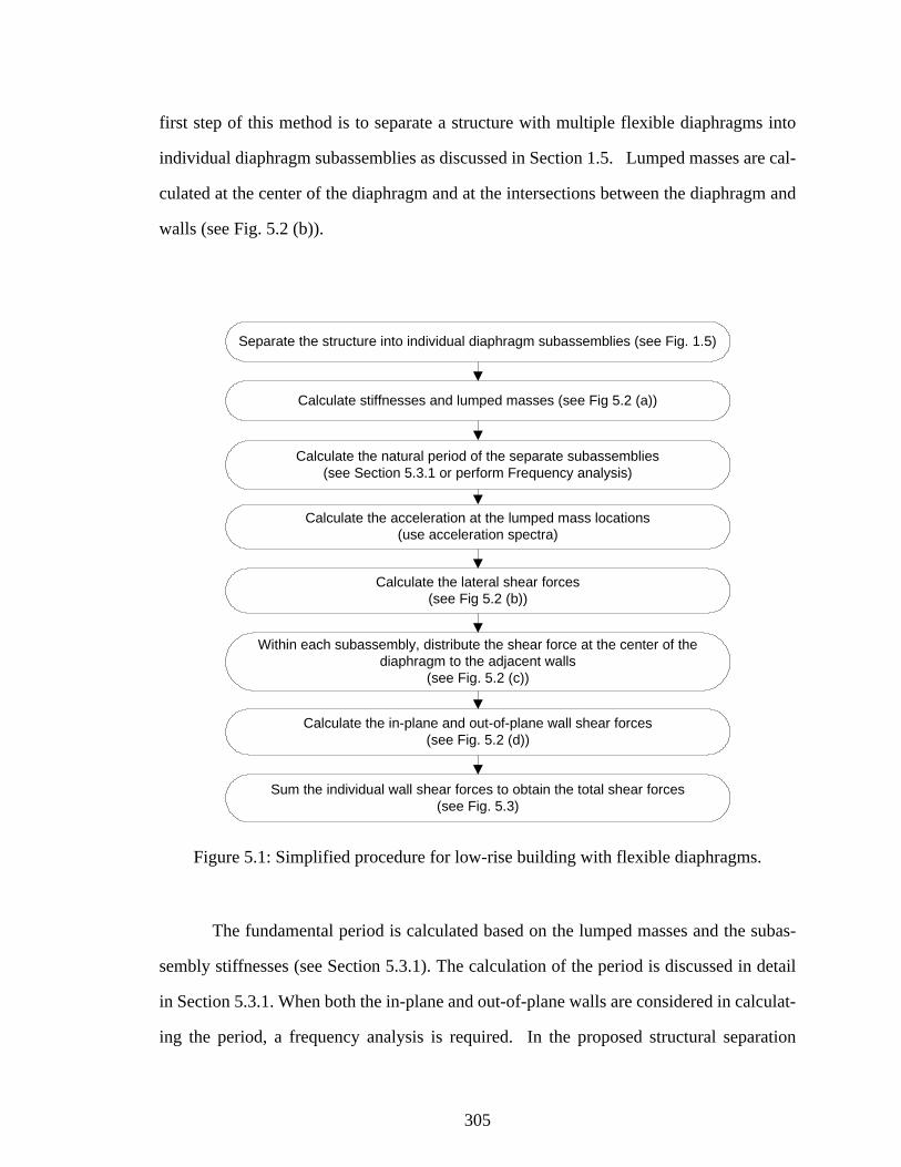
305

first step of this method is to separate a structure with multiple flexible diaphragms into

individual diaphragm subassemblies as discussed in Section 1.5. Lumped masses are cal-

culated at the center of the diaphragm and at the intersections between the diaphragm and

walls (see Fig. 5.2 (b)).

Figure 5.1: Simplified procedure for low-rise building with flexible diaphragms.

The fundamental period is calculated based on the lumped masses and the subas-

sembly stiffnesses (see Section 5.3.1). The calculation of the period is discussed in detail

in Section 5.3.1. When both the in-plane and out-of-plane walls are considered in calculat-

ing the period, a frequency analysis is required. In the proposed structural separation

Separate the structure into individual diaphragm subassemblies (see Fig. 1.5)

Calculate stiffnesses and lumped masses (see Fig 5.2 (a))

Calculate the natural period of the separate subassemblies(see Section 5.3.1 or perform Frequency analysis)

Calculate the acceleration at the lumped mass locations(use acceleration spectra)

Calculate the lateral shear forces(see Fig 5.2 (b))

Within each subassembly, distribute the shear force at the center of thediaphragm to the adjacent walls

(see Fig. 5.2 (c))

Calculate the in-plane and out-of-plane wall shear forces(see Fig. 5.2 (d))

Sum the individual wall shear forces to obtain the total shear forces(see Fig. 5.3)

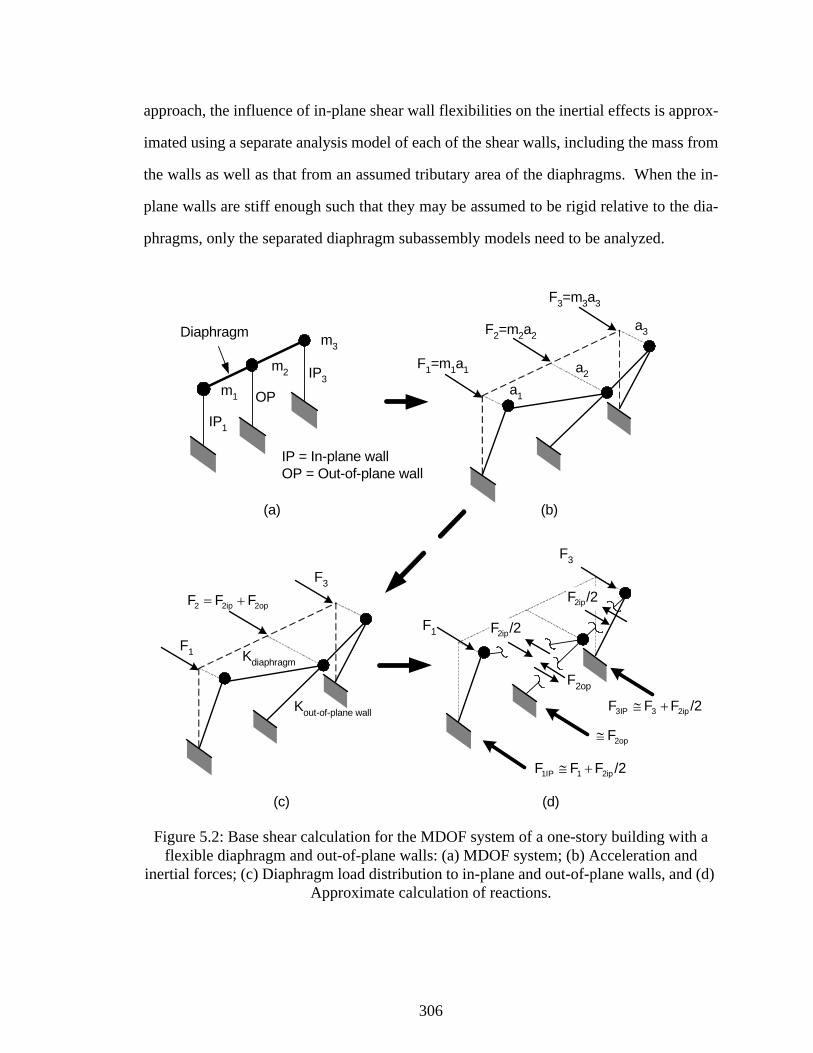
306

approach, the influence of in-plane shear wall flexibilities on the inertial effects is approx-

imated using a separate analysis model of each of the shear walls, including the mass from

the walls as well as that from an assumed tributary area of the diaphragms. When the in-

plane walls are stiff enough such that they may be assumed to be rigid relative to the dia-

phragms, only the separated diaphragm subassembly models need to be analyzed.

Figure 5.2: Base shear calculation for the MDOF system of a one-story building with a flexible diaphragm and out-of-plane walls: (a) MDOF system; (b) Acceleration and

inertial forces; (c) Diaphragm load distribution to in-plane and out-of-plane walls, and (d) Approximate calculation of reactions.

Diaphragm m3

m1

m2

IP1

IP3

OP

IP = In-plane wallOP = Out-of-plane wall

(a) (b)

(c) (d)

Kdiaphragm

F3

2op2ip2 FFF +=

F1

Kout-of-plane wall

F3

F1

/2FFF 2ip33IP +≅

2opF≅

/2FFF 2ip11IP +≅

F2op

/2F2ip

/2F2ip

a1

a2

a3

F1=m1a1

F2=m2a2

F3=m3a3

307

Figure 5.3: Approximate calculation of lateral forces of the two-story building with flexible diaphragms.

The accelerations at the lumped mass locations are determined using either

smoothed design or specific response spectra (see Section 5.3.2). The lateral forces are

calculated in the manner shown in Fig. 5.2 (b). The diaphragm lateral forces are distrib-

uted to the adjacent in-plane and out-of-plane walls (see Fig. 5.2 (c)). The base lateral

forces of the separated subassemblies are calculated (see Fig. 5.2 (c)) and summed to

obtain the total base shear of the structure with multiple diaphragms (see Fig. 5.3). The

detailed calculation of the lateral forces is discussed in Section 5.3.2.

5.3.1 Approximate period calculation for the separated diaphragm subassemblies

The approximate fundamental period calculation for a single-story structure with a

single nonrigid diaphragm is discussed in FEMA 273 and 356 (ASCE 2000a). FEMA 356

provides the following equation:

F1F2

F3F4

F5

F6

F7

F8F9

F102FF 2

1 +≅

2FFFF 72

61+

++≅

2FFFFFF 9742

83+++

++≅

2FFFF 94

105+

++≅

: Inertia force at lumped mass location: In-plane wall shear force

South wallCentral wall

North wallSouthdiaphragm

Northdiaphragm

1st story

2nd story

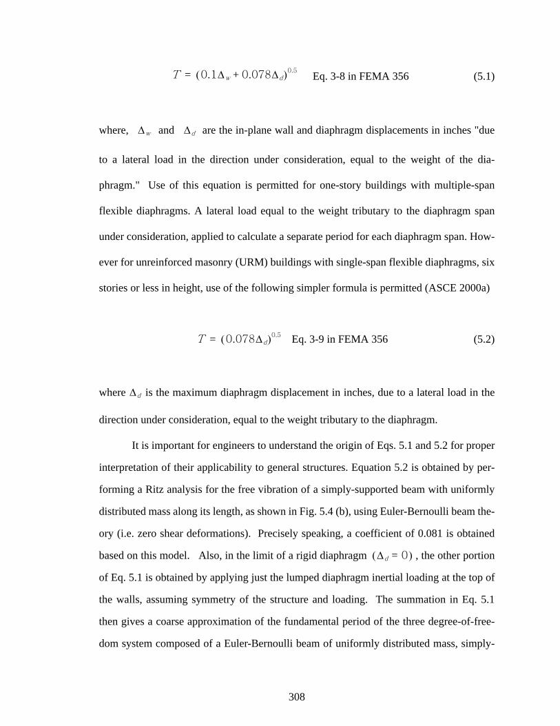
308

Eq. 3-8 in FEMA 356 (5.1)

where, and are the in-plane wall and diaphragm displacements in inches "due

to a lateral load in the direction under consideration, equal to the weight of the dia-

phragm." Use of this equation is permitted for one-story buildings with multiple-span

flexible diaphragms. A lateral load equal to the weight tributary to the diaphragm span

under consideration, applied to calculate a separate period for each diaphragm span. How-

ever for unreinforced masonry (URM) buildings with single-span flexible diaphragms, six

stories or less in height, use of the following simpler formula is permitted (ASCE 2000a)

Eq. 3-9 in FEMA 356 (5.2)

where is the maximum diaphragm displacement in inches, due to a lateral load in the

direction under consideration, equal to the weight tributary to the diaphragm.

It is important for engineers to understand the origin of Eqs. 5.1 and 5.2 for proper

interpretation of their applicability to general structures. Equation 5.2 is obtained by per-

forming a Ritz analysis for the free vibration of a simply-supported beam with uniformly

distributed mass along its length, as shown in Fig. 5.4 (b), using Euler-Bernoulli beam the-

ory (i.e. zero shear deformations). Precisely speaking, a coefficient of 0.081 is obtained

based on this model. Also, in the limit of a rigid diaphragm , the other portion

of Eq. 5.1 is obtained by applying just the lumped diaphragm inertial loading at the top of

the walls, assuming symmetry of the structure and loading. The summation in Eq. 5.1

then gives a coarse approximation of the fundamental period of the three degree-of-free-

dom system composed of a Euler-Bernoulli beam of uniformly distributed mass, simply-

T 0.1∆w 0.078∆d+( )0.5=

∆w ∆d

T 0.078∆d( )0.5=

∆d

∆d 0=( )

309

supported on flexible transverse springs (representing the wall flexibilities). Equation 5.2

effectively predicts the diaphragm natural period for the case of rigid structural walls.

Figure 5.4: Displacements of one bay one-story building with a flexible diaphragm.

It should be noted that if the natural period of the diaphragm is calculated based on

lumping of the mass at the diaphragm mid-span, as shown in Fig. 5.4 (d), a Ritz analysis

predicts a coefficient of 0.1 instead of 0.078 in Eqs. 5.2 and 5.4. This is obtained as:

∆d

Diaphragm

∆d

∆w

∆d

Diaphragm

Out-of-planewall

∆d

∆w

(c) (d)

(e) (f)

Out-of-planewall

∆d

∆w

∆d

Diaphragm

(a) (b)

310

(5.3)

(5.4)

FEMA 356 suggests that the diaphragm displacement, shown in Fig. 5.4 (a)

and (b), should be based on the likely distribution of the inertial forces, and suggests a par-

abolic distribution with a maximum magnitude of 1.5 Fd/L, where Fd is the total inertial

load applied to the diaphragm, for the equivalent static loading. FEMA 356 gives an illus-

tration similar to that of Fig. 5.4 (a) implying that only the diaphragm stiffness need be

included in the calculation of the diaphragm bending displacements.

The FEMA 356 model associated with Eq. 5.1 is reasonable for structures in which

the out-of-plane wall stiffnesses are negligible. However, the use of lumped masses is

more convenient and is considered to be sufficiently accurate for buildings in which there

are significant stiffness and strength contributions from both the in-plane and out-of-plane

walls, such as shown in Fig. 5.4(c) and in more general cases in which there are significant

three-dimensional (torsional) responses. This model simplifies to the one shown in Fig.

5.4(d) when the in-plane walls are assumed to be rigid. The inertial effects of the in-plane

wall masses do not influence the period, if the in-plane walls are effectively rigid, but, are

important to calculate the in-plane wall forces. Furthermore, it should be recognized that,

in general, both the mass as well as the stiffness of the out-of-plane walls influences the

response significantly. The mass of the masonry walls is typically much higher than that

of the diaphragm, and the behavior of the diaphragm generally includes a contribution

from the out-of-plane walls, as shown in Fig. 5.4 (e). The added mass from out-of-plane

shear walls increases the natural period and the stiffness of out-of-plane walls decreases

the natural period. Therefore, the models shown in Figs. 5.4 (e) and (f) are a more accu-

T 2π mk-----=

T 2π m

mg∆d

--------⎝ ⎠⎛ ⎞-------------- 0.1∆d( )0.5≅=

∆d

311

rate representation of this type of structure in general than those shown in Figs. 5.4 (a) and

(b). In light of the various approximations associated with the representation of the type

of structure considered in these figures, the period calculation using Eq. 5.3 is preferred.

However, if Equations 5.1 or 5.2 are employed, in general both the mass as well as the

stiffness of the out-of-plane walls should be included in the calculation of ∆d.

5.3.2 Lateral load calculations

5.3.2.1 Lateral load calculation within the separated subassemblies

Figure 5.2 (a) shows an individual isolated diaphragm subassembly separated from

a multi-story structure with multiple diaphragms. When the in-plane shear walls con-

nected to the diaphragm have significantly larger stiffness than that of the diaphragm and

the stiffness of the out-of-plane wall is negligible (e.g., the approximation suggested by

FEMA 356 for typical unreinforced masonry walls), the subassembly can be idealized as

shown in Fig. 5.4(d). When the stiffness of the out-of-plane walls is not negligible (i.e.,

reinforced masonry walls), the subassembly can be idealized as shown in Fig. 5.4(f) and

the stiffness contribution from the out-of-plane wall is included to calculate the natural

period. In either case, based on the assumption that the acceleration at the top of the in-

plane walls is equal to that at the base (i.e., rigid in-plane walls), the acceleration at the

center of the diaphragm is determined using either smoothed design or specific response

spectra in conjunction with the estimated period of vibration (see Section 5.3.1).

The lateral forces at the diaphragm level are calculated from the lumped mass and

acceleration at each DOF location, as shown in Fig. 5.2 (b). The lateral force at the center

of the diaphragm (see Fig. 5.2 (c)) is written as

(5.5)

F2

F2 F2ip F2op+=

312

where = lateral force distributed to the in-plane wall

= lateral force distributed to the out-of-plane wall

Based on the relative stiffness of the diaphragm and the out-of-plane walls, the lat-

eral force distribution to the in-plane and out-of-plane walls is calculated as

(5.6)

(5.7)

The lateral forces of the in-plane walls (see Fig. 5.2 (d)) are finally determined as

(5.8)

(5.9)

5.3.2.2 Total in-plane and out-of-plane wall lateral force calculation

Figure 5.3 shows the approximate calculation of the total shear wall forces for an

example two-story two-bay building with flexible diaphragms. It is assumed that the stiff-

nesses of the out-of-plane walls are negligible in this example (e.g., unreinforced masonry

walls or shear walls with large openings). The lateral forces at the center of the dia-

phragms, calculated from the separated subassemblies, are distributed and added to the

lateral forces from the lumped mass models at the tops of the adjacent shear walls. That

is, the lateral force at the second story in the south wall is the sum of the inertia force of

F2ip

F2op

F2op

F2

1Kdiaphragm

Kout-of-plane wall

----------------------------------+--------------------------------------------=

F2ip

F2

1Kout-of-plane wall

Kdiaphragm

----------------------------------+--------------------------------------------=

F1ip F1

F2ip

2---------+=

F3ip F3

F2ip

2---------+=

313

the second story in the south wall (F1) and the half of the inertia force from the lumped

mass at the center of the south roof diaphragm (F2). The wall lateral forces from the upper

story add to those from the lower story.

If out-of-plane walls are considered in a multiple story structure such as the exam-

ple shown in Fig. 5.3, the lateral load distribution discussed above will be more complex.

In this case, the lateral force distribution at the center of the diaphragms is influenced sig-

nificantly by the rigidity of the diaphragms and out-of-plane walls. When the proposed

structural separation method is applied to multiple-story structures, any coupling between

diaphragms that are located one above the other is neglected and it is assumed that the out-

of-plane wall stiffness effects are small relative to the diaphragm stiffness. Otherwise, the

subassembly concept must be modified.

5.4 Application of linear static procedure to the one-story CERL test building

In this example, the one-story half-scale test building, which is assessed in Chapter

IV, is studied using the proposed simplified linear static procedure outlined in the Section

5.3. This building is investigated in the manner shown in Fig. 5.2. The mass properties are

the same as those of the time history analysis model in Section 4.3.5. The effective damp-

ing is taken equal to 3% for the diaphragm subassembly, and an effective damping of 10%

is used for the in-plane masonry walls in the E-W direction, as discussed in Section 4.3.6.

The out-of-plane walls are included in this assessment as illustrated in Fig. 5.2. Test 3, one

of the three experimental tests of the test building considered in Chapter IV, is used to

investigate the simplified procedure, and the results from linear time history analysis are

compared with those of the simplified method.

314

5.4.1 Acceleration spectra

In order to assess the one-story low-rise building, a set of acceleration response

spectra that represent the earthquake motions used in the test are employed. The artifi-

cially scaled ground motion developed by Wen and Wu (1999) is used for test 3 (PGA =

0.5g). The acceleration spectra are obtained using the representative 2% in 50 years artifi-

cial ground motion (C02_09s) for that site. The acceleration spectra are calculated using

the Utility Software for Earthquake Engineering (USEE Version 0.9.8) developed by

Aschheim et al. (1999). Figures 5.5 and 5.6 show the half-time-scaled and unscaled accel-

eration spectra for various damping ratios. The test building was a half-scale model

whose natural periods are one-half those of the full-scale prototype structure. Thus, in

order to investigate the building using the simplified linear static procedure, the accelera-

tion spectra are obtained using the half-scaled input time that was used in the experimental

tests. The results of the simplified procedure using these spectra are compared with linear

time history analysis results of the test.

315

Figure 5.5: Half-time-scaled acceleration response spectra of 2% in 50 years Carbondale, IL artificial ground motion (C02_09s) for representative soil profile.

0.0

0.5

1.0

1.5

2.0

2.5

0 0.5 1 1.5 2

Period (sec)

Spec

tral

Res

pons

e A

ccel

erat

ion

(g)

2%3%5%7%10%

316

Figure 5.6: Half-time-scaled acceleration response spectra of 2% in 50 years Carbondale, IL artificial ground motion (C02_09s) for representative soil profile, plotted over a period

range of zero to 0.15 sec.

5.4.2 Force calculation

The lateral forces calculated at the top of in-plane walls and the center of the dia-

phragm are shown in Table 5.1. The period of the diaphragm subassembly is calculated

including the out-of-plane walls and assuming rigid in-plane walls, as shown in Fig.

5.4(f). The stiffnesses of diaphragm and out-of-plane wall are 7.41 and 16 kips/in, respec-

tively, as shown in Table 4.13. The weight at the center of the diaphragm is 1,519 lb. The

period is 0.082 sec calculated from Eq. 5.4. Equations 5.1 and 5.2 are not comparable

because the natural periods is a coarse approximation based on the maximum diaphragm

displacement. The acceleration, 1.32g shown in Table 5.1, is obtained from the accelera-

tion spectrum, as shown in Fig. 5.6, corresponding to the period (0.082 sec) and 3% damp-

0.0

0.5

1.0

1.5

2.0

2.5

0 0.05 0.1 0.15

Period (sec)

Spec

tral

Res

pons

e A

ccel

erat

ion

(g) 2%

3%5%7%10%

317

ing.

Two different calculations are considered for the periods of the north and south in-

plane walls. The first and most basic calculation is based on the simple assumption that

the in-plane walls are rigid, in which case, the accelerations at the tops of these walls are

the same as the wall base accelerations (PGA of 0.5 g). The second calculation is based

on the assumption of that the diaphragms are rigid. In this analysis, the finite in-plane and

out-of-plane wall stiffnesses are included and the period (0.056 sec in the third column in

Table 5.1) is calculated using the Ritz method considering the mass at the roof level and

the stiffness from the in-plane and out-of-plane walls (see the note under Table 5.1). The

spectral acceleration obtained from this analysis is 0.62g at the top of the in-plane walls.

This is somewhat larger than the PGA of 0.5g.

The lateral forces shown in the fifth column in Table 5.1 are calculated in the man-

ner shown in Fig. 5.2 (b). The lateral force at the center of the diaphragm (2.01 kips) is

distributed to the in-plane and out-of-plane walls using Eqs. 5.6 and 5.7. The lateral force

of the out-of-plane walls is 1.37 kips. The lateral force of the in-plane wall, including the

contribution from the lateral force at the center of the diaphragm, is 0.95 kips. The total

lateral forces at the base are shown in the sixth column of the Table 5.1.

318

Table 5.1: Calculated lateral forces from the simplified linear static procedure in the E-W direction.

a. Max inertial loads (F1, F2, and F3) in Fig. 5.2(b).b. Wall shear forces (F1IP, F2OP, and F3IP) in Fig. 5.2(d).c. PGA assuming rigid in-plane shear walls.d. Period calculated from the Ritz method assuming rigid diaphragm (K = Kop + 2 Kip = 116 kip/in, M = 9.26 (lb sec2/in).e. Analysis results from linear time history analysis (see Table 4.9).

5.4.3 Comparison of the simplified procedure and linear time history analysis

Table 5.2 compares the lateral base shear forces from the simplified procedure (see

Table 5.1) and linear time history analysis (see Table 4.11). The in-plane wall lateral force

from the simplified procedure (0.95 kips) matches well with the one from the linear time

history analysis (0.91 kips). The out-of-plane wall force (1.37 kips) is somewhat smaller

than the one from the linear time history analysis (1.61 kips).

The lateral forces shown in the fifth column in Table 5.1 are applied to the CERL

LocationMass (lb-sec2/in)

Period(sec)

Acceleration (g)

Max. inertial loadsa (kips)

Wall shear forcesb (kips)

South wall 2.66 0.056b0.50c

0.62d

0.70e

0.52c

0.64d0.84c

0.95d

out-of-plane wall (at the center of the

diaphragm)3.94 0.082

1.32 1.45e 2.01 1.37

North wall 2.66 0.056b0.50c

0.62d

0.70e

0.52c

0.64d0.84c

0.95d

319

test building model (see Figs. 4.6 and 5.2 (b)) and a linear static analysis is performed to

calculate the displacements. The static analysis differs from these of the simplified proce-

dure results due to the lateral load distribution from the center of the diaphragm to the in-

plane and out-of-plane walls. These results are closer to the time history analysis results

than those of the simplified procedure. The results of the linear static analysis match well

with those of the linear time history analysis, as shown in Fig. 5.7 and Table 5.2, although

the lateral force (1.49 kips) at the out-of-plane wall is slightly underestimated compared to

that (1.61 kips) of the linear time history analysis. The north and south wall reaction

forces (0.90 kips) compare with the peak reaction forces (0.913 kips) calculated from the

linear time history analysis, as shown in Fig. 5.8. The out-of-plane wall reaction force is

compared in Fig. 5.9. The in-plane and out-of-plane displacements (0.018 and 0.093 in,

respectively) are matched well with the peak displacements (0.02 and 0.1 in, respectively)

from the linear time history analysis (see Table 5.2). The results of the simplified proce-

dure are considered accurate in spite of its simplicity.

Table 5.2: Comparison of analysis results.

Location

Simplified procedure Linear static analysis Linear time history

analysis

Force (kips)

Force (kips)

Disp.(in)

Force (kips)

Disp.(in)

South wall 0.95 0.90 0.018 0.91 0.02

Out-of-plane wall 1.37 1.49 0.093 1.61 0.10

North wall 0.95 0.90 0.018 0.91 0.02

320

Figure 5.7: Comparison of analysis results.

Figure 5.8: Comparison of reaction forces at the south and north wall.

0.0

0.5

1.0

1.5

2.0

1 2 3

Location

Rea

ctio

n fo

rce

(kip

s)

Linear static analysis

Linear time historyanalysis

Southwall

Northwall

Out-of-planewall

0.0

0.5

1.0

1.5

0 2 4 6 8 10

Time (sec)

Abs

olut

e re

actio

n fo

rce

(kip

s)

Time history analysis

Linear static procedure

321

Figure 5.9: Comparison of reaction forces at out-of-plane wall.

5.5 Application of linear static procedure to the Gilroy firehouse using structural

separation method

The main purpose of this assessment is to investigate the applicability of the sim-

plified procedure discussed in Section 5.2 for a multi-story building with multiple flexible

diaphragms. The two-story URM shear wall building with flexible diaphragms investi-

gated in Chapter III is used to demonstrate the structural separation method and apply the

simplified linear static procedure.

Section 5.5.1 compares the time history analysis results using the structural separa-

tion method with those from the model of the complete two-story structure. Section 5.5.2

shows the comparison of the simplified procedure and the linear time history analysis

results.

5.5.1 Validation of the structural separation method

The structural separation method (see Section 5.2.3) is applied to the two-story

0

1

2

0 2 4 6 8 10Time (sec)

Abs

olut

e re

actio

n fo

rce

(kip

s)

Time history analysis

Linear static procedure

322

building with multiple diaphragms (see Fig. 3.1). Linear time history analyses are per-

formed using each one-story single diaphragm subassembly. The summed reaction forces

and displacements from the subassembly analyses are compared with the results from the

complete building model.

Section 5.5.1.1 explains how the two-story structure is separated into the single-

story single-bay subassemblies. Section 5.5.1.2 discusses the validation of the structural

separation method by comparing the linear time history analysis results from the separated

subassemblies with the results from the analysis of the complete two-story building.

5.5.1.1 Structural separation of the two-story building with multiple diaphragms

The response of two-story building (see Fig. 3.1) is considered into the separate

the E-W and N-S directions (see Figs. 5.10 and 5.11). The out-of-plane URM walls are

neglected in these models. The lumped masses are located at the center of the diaphragm

and the top of the shear walls. The structure is displaced due to the lateral seismic ground

motion in the E-W and N-S directions, as shown in Figs. 5.10 and 5.11.

The first four mode shapes from the eigenvalue analysis of the building are shown

in Fig. 3.23. As discussed in Section 3.4.1, it appears that the flexible diaphragms have

considerably smaller stiffnesses compared to the stiffnesses of masonry walls. The dia-

phragms effectively respond independently of one another. Based on this observation, the

structural separation method of the building can be considered. The structural separation

(see Figs. 5.10 and 5.11) is based on the one-story subassemblies with single diaphragm.

The separate models in Figs. 5.10 and 5.11 are used to calculate their natural periods. The

story shear forces of the buildings are calculated at the lumped mass locations on each dia-

phragm. The natural periods are used to calculate the maximum inertial forces at the cen-

ter of the diaphragms. The maximum inertial forces at the top of the in-plane walls are

calculated from the peak accelerations at the top of the in-plane walls. In this section,

these peak accelerations are assumed to be equal to the PGA.

323

Figure 5.10: Structural separation of the two-story building in the E-W direction.

+

1st Story

Model A1S Model A1N

2nd Story

+

Model A2S Model A2N

+

3D Model

2D Model (E-W direction)

South Diaphragm

m1m2

m3m4 m5

m6

m7

m8

m9m10

North Diaphragm

South Wall

Central Wall

East Wall

West WallRoof

2nd Floor

Ground floor

North Wall

m1

m2

m3

m5m4

m6

m7

m8

m9 m10

Model A1 Model A2

324

Figure 5.11: Structural separation of the two-story building in the N-S direction.

5.5.1.2 Comparison of linear time history analysis results

The purpose of these comparisons with the results of two-story building model is

to assess if the building can be separated into the subassemblies (see Figs. 5.10 and 5.11)

at each story level. In order to assess the independent behavior of the multiple flexible dia-

phragms in the building, time history analyses are performed to obtain the response of the

m21

East Wall

West WallRoof

2nd Floor

Ground floor

m22 m23

m24m25 m26

3D Model

2D Model (N-S direction) m21

m22

m23

m24

m25m26

2nd Story1st Story

Model A1 Model A2

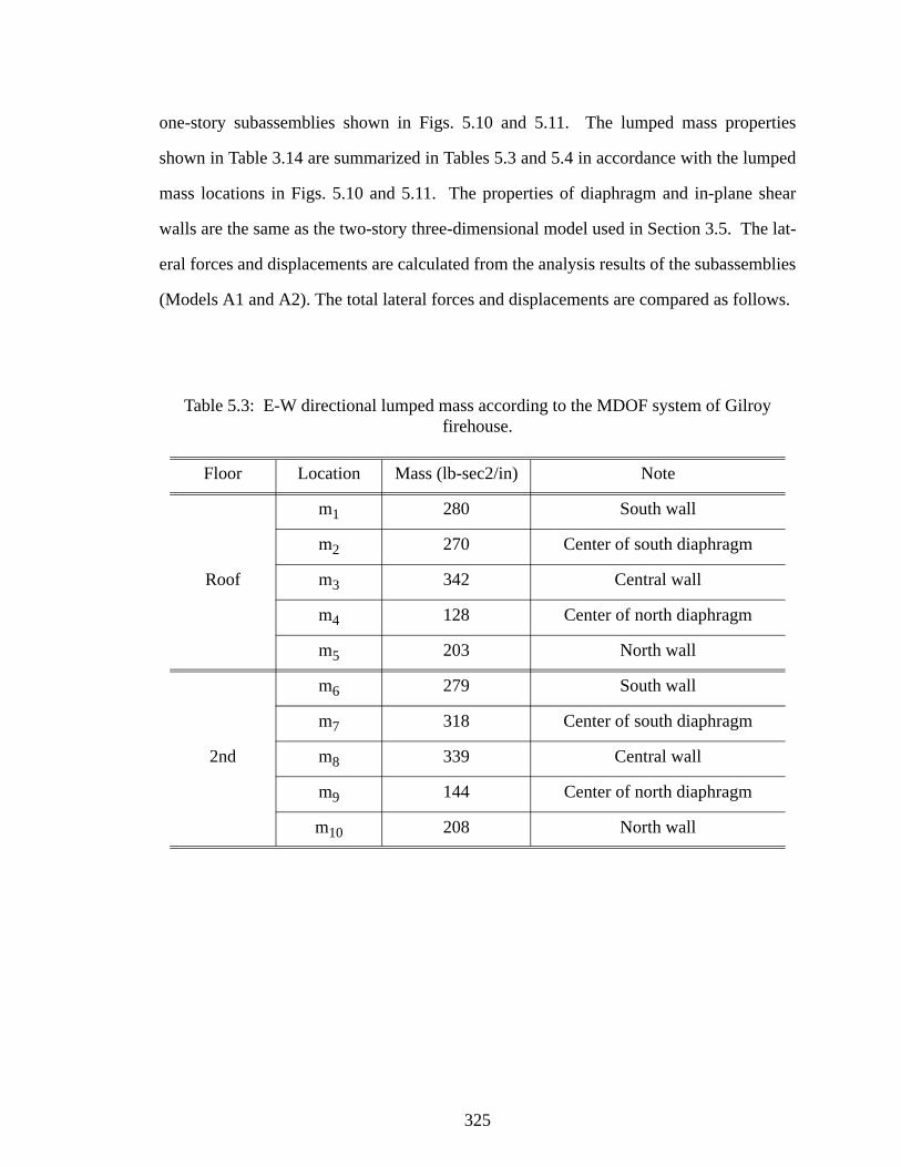
325

one-story subassemblies shown in Figs. 5.10 and 5.11. The lumped mass properties

shown in Table 3.14 are summarized in Tables 5.3 and 5.4 in accordance with the lumped

mass locations in Figs. 5.10 and 5.11. The properties of diaphragm and in-plane shear

walls are the same as the two-story three-dimensional model used in Section 3.5. The lat-

eral forces and displacements are calculated from the analysis results of the subassemblies

(Models A1 and A2). The total lateral forces and displacements are compared as follows.

Table 5.3: E-W directional lumped mass according to the MDOF system of Gilroy firehouse.

Floor Location Mass (lb-sec2/in) Note

Roof

m1 280 South wall

m2 270 Center of south diaphragm

m3 342 Central wall

m4 128 Center of north diaphragm

m5 203 North wall

2nd

m6 279 South wall

m7 318 Center of south diaphragm

m8 339 Central wall

m9 144 Center of north diaphragm

m10 208 North wall

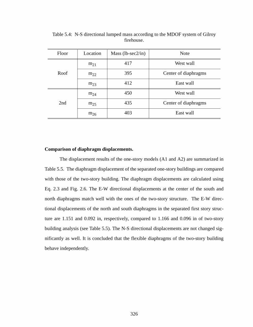
326

Table 5.4: N-S directional lumped mass according to the MDOF system of Gilroy firehouse.

Comparison of diaphragm displacements.

The displacement results of the one-story models (A1 and A2) are summarized in

Table 5.5. The diaphragm displacement of the separated one-story buildings are compared

with those of the two-story building. The diaphragm displacements are calculated using

Eq. 2.3 and Fig. 2.6. The E-W directional displacements at the center of the south and

north diaphragms match well with the ones of the two-story structure. The E-W direc-

tional displacements of the north and south diaphragms in the separated first story struc-

ture are 1.151 and 0.092 in, respectively, compared to 1.166 and 0.096 in of two-story

building analysis (see Table 5.5). The N-S directional displacements are not changed sig-

nificantly as well. It is concluded that the flexible diaphragms of the two-story building

behave independently.

Floor Location Mass (lb-sec2/in) Note

Roof

m21 417 West wall

m22 395 Center of diaphragms

m23 412 East wall

2nd

m24 450 West wall

m25 435 Center of diaphragms

m26 403 East wall

327

Table 5.5: Comparison of peak relative diaphragm displacements for the subassemblies (see Fig. 5.10) and the complete two-story building.

Comparison of in-plane wall lateral forces.

Table 5.6 shows the comparison of the lateral forces of the in-plane masonry walls.

The summed in-plane wall lateral forces of the subassemblies match well with those of the

second story building. The sum of the south wall lateral force (60 kips) in Model A2 and

the lateral force (62 kips) in Model A1 match well with the shear reaction (130 kips) at the

south wall of the two-story structure. It is concluded that the in-plane lateral forces of the

two-story building can be calculated accurately by summing the in-plane forces calculated

from the subassemblies and using the structural separation method.

Direction Floor LocationDiaphragm displacement (in)

Model A2 Model A1 Complete MDOF model

E-W

RoofSouth 1.123

-1.142

North 0.083 0.088

2ndSouth

-1.151 1.166

North 0.092 0.096

N-S

RoofSouth 0.401

-0.414

North 0.401 0.414

2ndSouth

-0.579 0.598

North 0.579 0.598

328

Table 5.6: Comparison of shear wall displacement and lateral force for the subassemblies (see Fig. 5.10) and the complete two-story building (unit: kips).

5.5.2 Calculations using the simplified linear static procedure

The individual models of Step A in Figs. 5.10 and 5.11 are analyzed to check the

lateral forces using the simplified linear static procedure. The results calculated from the

subassemblies are compared to those of the linear time history analysis to assess the qual-

ities and limitations of the procedures for low-rise multiple story buildings with multiple

flexible diaphragms.

5.5.2.1 Acceleration spectra

The two recorded ground motions in the E-W (U3) and the N-S direction (U1) are

measured at the base of the two-story building (see Section 3.2). These records are used to

derive acceleration spectra for different levels of damping from 2 to 10%. The accelera-

tion spectra, as shown in Figs. 5.12 and 5.15, are calculated using Utility Software for

Direction Story Location Model A2

Model A1

Reaction forces (A1+A2)

Complete MDOF model

E-W

2nd

South 60

- -

65

Central 66 66

North 30 32

1st

South

-

62 122 130

Central 69 135 135

North 31 61 64

N-S2nd

East 74 - -

76

West 76 76

1stEast

-64 138 145

West 71 147 149

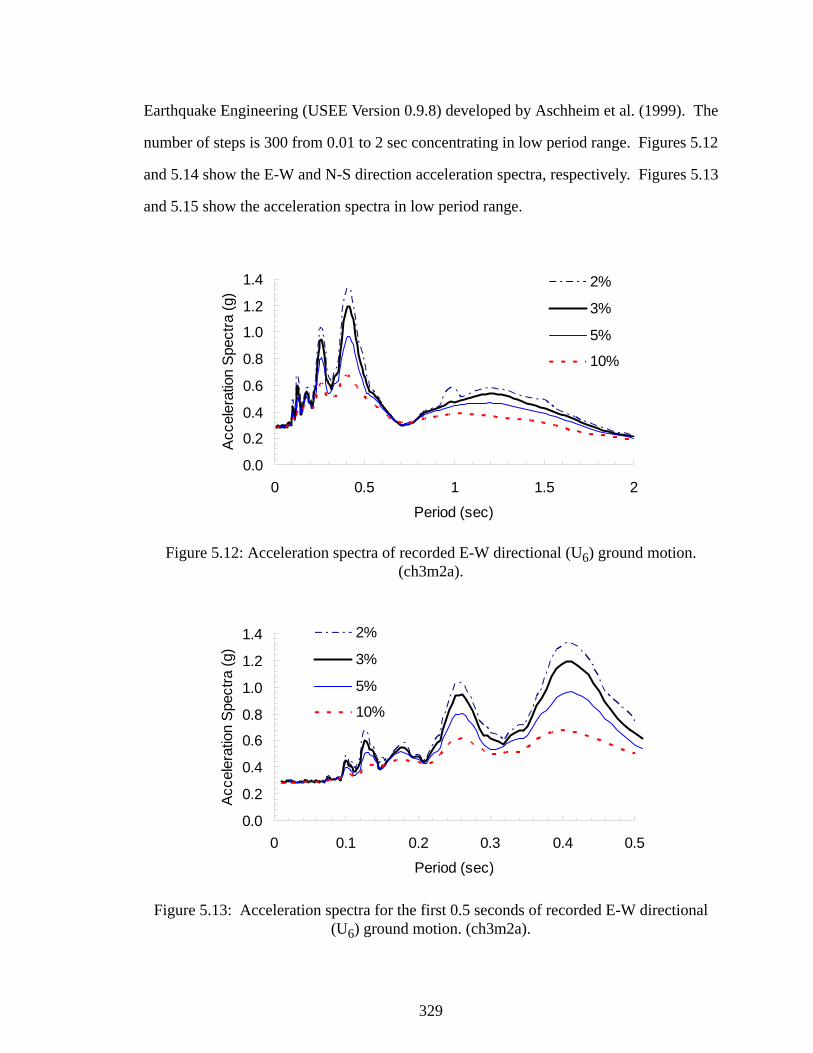
329

Earthquake Engineering (USEE Version 0.9.8) developed by Aschheim et al. (1999). The

number of steps is 300 from 0.01 to 2 sec concentrating in low period range. Figures 5.12

and 5.14 show the E-W and N-S direction acceleration spectra, respectively. Figures 5.13

and 5.15 show the acceleration spectra in low period range.

Figure 5.12: Acceleration spectra of recorded E-W directional (U6) ground motion. (ch3m2a).

Figure 5.13: Acceleration spectra for the first 0.5 seconds of recorded E-W directional (U6) ground motion. (ch3m2a).

0.0

0.2

0.4

0.6

0.8

1.0

1.2

1.4

0 0.5 1 1.5 2

Period (sec)

Acc

eler

atio

n Sp

ectra

(g)

2%

3%

5%

10%

0.0

0.2

0.4

0.6

0.8

1.0

1.2

1.4

0 0.1 0.2 0.3 0.4 0.5

Period (sec)

Acce

lera

tion

Spec

tra (g

)

2%

3%

5%

10%

330

Figure 5.14: Acceleration spectra of recorded N-S directional (U1) ground motion. (ch1m2a).

Figure 5.15: Acceleration spectra for the first 0.5 seconds of recorded N-S directional (U1) ground motion. (ch1m2a).

5.5.2.2 Force calculation

For the assessment of the building in the E-W and N-S direction (see Figs. 5.10

and 5.11), natural periods of the separated subassemblies are calculated. The diaphragm

stiffness and the lumped masses at the center of the diaphragms (see Tables 5.7 and 5.8)

0.0

0.2

0.4

0.6

0.8

1.0

0 0.5 1 1.5 2

Period (sec)

Acc

eler

atio

n Sp

ectra

(g) 2%

3%

5%

10%

0.0

0.2

0.4

0.6

0.8

1.0

0 0.1 0.2 0.3 0.4 0.5Period (sec)

Acc

eler

atio

n S

pect

ra (g

)

2%

3%

5%

10%

331

are used to calculate the period using the Ritz method. The E-W directional natural peri-

ods of the separated structures (A1S, A1N, A2S, and A2N in Fig. 5.10) are summarized in

Table 5.7 and the N-S directional natural periods of separated structures (see Fig. 5.11)

are summarized in Table 5.8. The stiffnesses of in-plane masonry walls are assumed to be

rigid for the approximate period calculation. The natural period (0.412 sec) calculated

from the south roof diaphragm subassembly is quite similar to the fundamental period

(0.415 sec) of the two-story MDOF model discussed in Chapter III.

The accelerations shown in Tables 5.9 and 5.10 are calculated from the response

spectra (see Figs. 5.13 and 5.15) for different levels of damping from 2 to 10%.

Table 5.7: Diaphragm period calculation of structures in the E-W direction.

Table 5.8: Diaphragm period calculation of structures in N-S direction.

Story ModelMass

(lb-sec2/in)Stiffness(kips/in)

Period(sec)

1stA1S 318 70 0.423

A1N 144 233 0.156

2ndA2S 270 62.7 0.412

A2N 128 233 0.147

StoryMass

(lb-sec2/in)Stiffness(kips/in)

Period (sec)

1st 435 136 0.355

2nd 395 176 0.298

332

Table 5.9: Acceleration obtained from response spectra shown in Fig. 5.13. .

Table 5.10: Acceleration obtained from response spectra shown in Fig. 5.15.

The lateral forces shown in Tables 5.11 and 5.12 are calculated by multiplying the

masses by the acceleration at lumped mass locations, (see Figs. 5.10 and 5.11). For sim-

plicity, the in-plane walls are assumed to be rigid and the acceleration at the tops of in-

plane masonry walls is assumed to be equal to the measured peak accelerations at these

bases. This is reasonable for a simplified procedure in this type of building. The accelera-

tions calculated from this simple assumption do not significantly differ from the measured

peak acceleration of the in-plane walls shown in the fourth column of Table 5.11. The

acceleration at the top of the south wall (0.319 g) is slightly higher than the measured peak

acceleration (0.29 g) in the E-W direction.

The lateral force (80 kips) at the center of the south diaphragm is much larger than

that of the in-plane wall lateral forces (31 kips). Half of the lateral force (80 kips) calcu-

lated at the center of the south diaphragm is distributed to the south and central shear walls

Story Structure Period(sec)

Acceleration (g)

3% damping 5% damping 10% damping

1stA1S 0.423 1.132 0.930 0.650

A1N 0.156 0.455 0.443 0.427

2ndA2S 0.412 1.188 0.966 0.665

A2N 0.147 0.412 0.388 0.408

Story Period(sec)

Acceleration (g)

3% damping 5% damping 10% damping

1st 0.355 0.575 0.522 0.455

2nd 0.298 0.755 0.630 0.471

333

as shown in Fig. 5.3. Half of the lateral forces calculated at the center of the north dia-

phragm (24 kips) are distributed to central and north walls. The in-plane wall lateral

forces are summarized in the sixth column of Tables 5.11 and 5.12 for the E-W and N-S

directional assessment, respectively.

334

Table 5.11: Calculated lateral forces from the linear static procedure in -E-W direction.

a. obtained from linear time history analysis of MDOF model.

Model Location Mass (lb-sec2/in)

Acceleration (g)

Max. inertial

loads (kips)

Wall shear forces (kips)

A1

South wall 2790.2900.319a 31 71

Center of south diaphragm 318

0.6500.672a 80 -

Central wall 3390.2900.299a 38 90

Center of north diaphragm 144

0.4270.431a 24 -

North wall 2080.2900.293a 23 35

A2

South wall 2800.2900.345a 31 66

Center of south diaphragm 270

0.6650.699a 69 -

Central wall 3420.2900.312a 38 83

Center of north diaphragm 128

0.4080.445a 20 -

North wall 2030.2900.309a 23 33

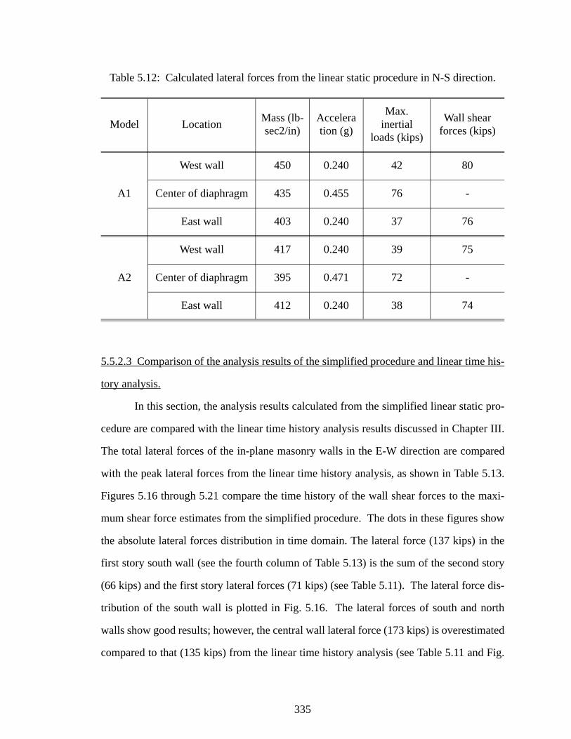
335

Table 5.12: Calculated lateral forces from the linear static procedure in N-S direction.

5.5.2.3 Comparison of the analysis results of the simplified procedure and linear time his-

tory analysis.

In this section, the analysis results calculated from the simplified linear static pro-

cedure are compared with the linear time history analysis results discussed in Chapter III.

The total lateral forces of the in-plane masonry walls in the E-W direction are compared

with the peak lateral forces from the linear time history analysis, as shown in Table 5.13.

Figures 5.16 through 5.21 compare the time history of the wall shear forces to the maxi-

mum shear force estimates from the simplified procedure. The dots in these figures show

the absolute lateral forces distribution in time domain. The lateral force (137 kips) in the

first story south wall (see the fourth column of Table 5.13) is the sum of the second story

(66 kips) and the first story lateral forces (71 kips) (see Table 5.11). The lateral force dis-

tribution of the south wall is plotted in Fig. 5.16. The lateral forces of south and north

walls show good results; however, the central wall lateral force (173 kips) is overestimated

compared to that (135 kips) from the linear time history analysis (see Table 5.11 and Fig.

Model Location Mass (lb-sec2/in)

Acceleration (g)

Max. inertial

loads (kips)

Wall shear forces (kips)

A1

West wall 450 0.240 42 80

Center of diaphragm 435 0.455 76 -

East wall 403 0.240 37 76

A2

West wall 417 0.240 39 75

Center of diaphragm 395 0.471 72 -

East wall 412 0.240 38 74

336

5.22).

The total lateral forces of the in-plane walls in the N-S direction are compared in

Table 5.14. Figures 5.23 to 5.26 compare the in-plane lateral forces of the simplified linear

static procedure and the shear force histories from the linear time history analyses. The

lateral forces in the east and west walls match well with those of linear time history analy-

sis (see Fig. 5.27 and Table 5.14). The lateral forces of the east and west walls (140 and

144 kips, respectively) are compared with those of the time history analysis (150 and 154

kips, respectively).

Table 5.13: Comparison of in-plane wall lateral forces in the E-W direction.

a. The peak lateral forces are obtained from the linear time history analysis of the two-story MDOF model discussed in Chapter III.b. Combined total lateral forces of walls calculated from Table 5.11, assuming that eachdiaphragm structure moves separately.

Story Wall (Position)Lateral forces (kips)

Linear time history analysisa Linear static procedureb

2nd

South (1) 65 66

Central (2) 66 83

North (3) 32 33

1st

South (1) 130 137

Central (2) 135 173

North (3) 64 68

337

Figure 5.16: Comparison of lateral force of south shear wall at first story.

Figure 5.17: Comparison of lateral force of central shear wall at first story.

020406080

100120140160

0 5 10 15 20Time (sec)

Abs

olut

e Sh

ear F

orce

(kip

s)

Time history analysis

Linear static procedure

0

50

100

150

200

0 5 10 15 20Time (sec)

Abs

olut

e Sh

ear F

orce

(kip

s)

Time history analysis

Linear static procedure

338

Figure 5.18: Comparison of lateral force of north shear wall at first story.

Figure 5.19: Comparison of lateral force of south shear wall at second story.

01020304050607080

0 5 10 15 20Time (sec)

Abs

olut

e Sh

ear F

orce

(kip

s)

Time history analysis

Linear static procedure

0

10

2030

40

50

60

70

0 5 10 15 20Time (sec)

Abs

olut

e Sh

ear F

orce

(kip

s)

Time history analysis

Linear static procedure

339

Figure 5.20: Comparison of lateral force of central shear wall at second story.

Figure 5.21: Comparison of lateral force of north shear wall at second story.

0102030405060708090

0 5 10 15 20Time (sec)

Abs

olut

e Sh

ear F

orce

(kip

s)

Time history analysis

Linear static procedure

0

5101520

25

3035

0 5 10 15 20Time (sec)

Abs

olut

e Sh

ear F

orce

(kip

s)

Time history analysis

Linear static procedure

340

Figure 5.22: Comparison of lateral forces in the E-W direction.

Table 5.14: Comparison of in-plane wall lateral forces in N-S direction.

a. The lateral forces are obtained from linear time history analysis of two-story MDOFmodel.b. Combined total base lateral forces of walls calculated from Table 5.11, assuming thateach diaphragm structure moves separately.

Story Wall (Position)Lateral forces (kips)

Linear time history analysisa Linear static procedureb

2nd East 76 74

West 77 76

1st East 140 150

West 144 154

0

45

90

1 2 3

Location

Tota

l Bas

e Sh

ear

(kip

s)

Linear static procedure

Linear time history analysis

0

90

180

1 2 3

Location

Tota

l Bas

e S

hear

(kip

s)

Southwall

Centralwall

Northwall

Southwall

Centralwall

Northwall

2nd Story 1st Story

341

Figure 5.23: Comparison of lateral force of east shear wall at first story.

Figure 5.24: Comparison of lateral force of west shear wall at first story.

020406080

100120140160

0 5 10 15 20Time (sec)

Abs

olut

e Sh

ear F

orce

(kip

s)

Time history analysis

Linear static procedure

020406080

100120140160180

0 5 10 15 20Time (sec)

Abs

olut

e Sh

ear F

orce

(kip

s)

Time history analysis

Linear static procedure

342

Figure 5.25: Comparison of lateral force of east shear wall at second story.

Figure 5.26: Comparison of lateral force of west shear wall at second story.

01020304050607080

0 5 10 15 20Time (sec)

Abs

olut

e Sh

ear F

orce

(kip

s)

Time history analysis

Linear static procedure

0

20

40

60

80

100

0 5 10 15 20

Time (sec)

Abs

olut

e Sh

ear F

orce

(kip

s)

Time history analysis

Linear static procedure

343

Figure 5.27: Comparison of lateral forces in N-S direction.

Tables 5.15 and 5.16 compare the displacements calculated from the simplified lin-

ear static procedure and linear time history analysis. The element displacements are cal-

culated from dividing lateral forces shown in Tables 5.11 and 5.13 by the stiffnesses

shown in Table 5.15. The displacement of the second story central wall (0.55 in) is over-

estimated as much as 20% compared to that of linear time history analysis (0.044 in). The

lateral force of the central wall (173 kips) is overestimated as much as 28 % compared to

that of linear time history analysis (135 kips) (see Table 5.13). However, the overall

responses match well with those of time history analysis in the E-W and N-S directions.

0

40

80

1 2

Location

Tota

l Bas

e S

hear

(kip

s)

Linear static procedure

Linear time history analysis

0

80

160

1 2

Location

Tota

l Bas

e S

hear

(kip

s)

Eastwall

2nd Story 1st Story

Westwall

Eastwall

Westwall

344

Table 5.15: Comparison of displacement in the E-W direction.

a. displacement obtained from the separated structure assuming that each structural com-ponents move separately. b. displacement at the top of walls and the center of diaphragms of the two-story building.c. displacement obtained from linear time history analysis of two-story MDOF model.

Story Location Stiffness (kips/in)

Simplified linear static procedure Linear time history

analysisc

(in)

Element displacementa

(in)

Nodal displacementb

(in)

2nd

South wall 1,654 0.040 0.108 0.103

Center of south diaphragm 63 1.105 1.136 1.218

Central wall 3,739 0.022 0.055 0.044

Center of north diaphragm 233 0.086 0.105 0.110

North wall 2,170 0.015 0.025 0.023

1st

South wall 2,008 0.068 0.068 0.064

Center of south diaphragm 70 1.140 1.190 1.216

Central wall 5,263 0.033 0.033 0.026

Center of north diaphragm 233 0.102 0.123 0.104

North wall 7,005 0.010 0.010 0.009

345

Table 5.16: Comparison of displacement in N-S direction.

a. displacement obtained from the separated structure assuming that each structural com-ponents move separately. b. displacement at the top of walls and the center of diaphragms of the two-story building.c. displacement obtained from linear time history analysis of two-story MDOF model.

5.6 Implications for General Seismic Assessment

The above analysis solutions are all based on linear elastic response. However, for

general seismic assessment, the influence of potential nonlinear structural actions must be

considered. Based on the above analysis results, it is apparent that the out-of-plane walls

are typically damaged at an early stage due to the relatively large out-of-plane displace-

ments associated with the flexible diaphragms. The authors are not aware of any research

that has investigated the in-plane hysteretic response of wall components that are simulta-

neously subjected to out-of-plane damage. Given this lack of knowledge about the wall

responses, it may be wise to consider in-plane unreinforced masonry walls as force-con-

trolled components, while handling the potentially significant out-of-plane hysteretic

Story Location Stiffness (kips/in)

Simplified linear static procedure Linear time history

analysisc

(in)

Element displacementa

(in)

Nodal displacementb

(in)

2nd

East wall 1,835 0.021 0.060 0.078

Center of diaphragm 176 0.408 0.425 0.453

West wall 6,038 0.012 0.028 0.027

1st

East wall 3,820 0.039 0.039 0.036

Center of diaphragm 136 0.562 0.589 0.613

West wall 9,806 0.016 0.016 0.015

346

response as a deformation-controlled problem. In the context of this philosophy, the appli-

cation of the structural separation method is relatively straightforward. The out-of-plane

walls can be handled using equivalent linear properties based on their expected response.

Alternatively, the effects of inelasticity might be incorporated in the calculation of

the lateral forces within the structural separation method, step 5 of Fig. 5.1, by using the

FEMA 356 pseudo lateral load equation in each of the subassemblies, that is Eq. (3-10) of

FEMA 356. In this case, appropriate modification factors C1, C2, C3 and Cm must be

determined. Further research is necessary to determine precisely what values should be

used for these coefficients in flexible diaphragm structures.

However, if one of in-plane walls in a story (e.g., one of the walls in the two story

building discussed in this paper) is damaged, the force distribution within the structural

system will tend to be significantly changed from that of the elastic model. For example,

if the south wall of the two-story building is severely damaged due to in-plane wall action,

a larger fraction of the south wall shear force is taken by the east, west, and central walls,

and a small fraction of the force is taken by the north wall due to the flexible diaphragm

(via shear raking within the south diaphragm and overall torsion of the structure). If the

central wall (interior wall) is severely damaged, a larger fraction of the central wall shear

is taken by all exterior walls. In these cases, the force or displacement calculation of the

walls and diaphragms can not be considered by using the simplified procedure discussed

in this chapter. In order to investigate such an extensively damaged structure, a nonlinear

dynamic analysis using the 3D MDOF model of Chapter II is recommended. The gravity

load within the structure must be included in this MDOF model.

5.7 Summary and Conclusion

A simplified linear static procedure for structures with flexible diaphragms, termed

the structural separation method is studied. Acceleration spectra calculated from the

347

recorded ground motions are used to determine the accelerations at the lumped mass loca-

tions. The natural periods of the diaphragms are obtained from the subassemblies assum-

ing rigid in-plane walls. The spectral accelerations at the tops of the in-plane walls are

calculated based on either of two idealizations as appropriate. The first idealization uses a

separate analysis model of each of the in-plane walls, including the mass from the walls as

well as that from an assumed tributary area of the diaphragms. The second idealization is

that the accelerations at the tops of the in-plane walls are equal to those at the base, based

on the assumption that the in-plane walls are rigid. The second idealization can be applied

to the in-plane walls in many shear wall structures with flexible diaphragms.

The wall lateral forces are obtained by summing the maximum values obtained

from the separate diaphragm subassemblies with those obtained from one of the two ideal-

izations of the in-plane walls. The calculated lateral forces match well with those of time

history analysis results. The following general conclusions can be made from this study.

• Low-rise shear wall buildings with nonrigid diaphragms do not behave as SDOF

systems. These types of buildings must be assessed as MDOF structures

explicitly considering the in-plane and out-of-plane walls associated with the

nonrigid diaphragms.

• The proposed simplified procedure can accurately and simply investigate the

response of buildings with flexible diaphragm including the out-of-plane wall

stiffness and mass. This method is predicated on the judgment that, due to the

fact that wall damage in the out-of-plane directions is likely to occur first and is

not easily prevented by retrofit measures, damage in the in-plane wall direc-

tions generally should be limited. The walls should be investigated as force-

controlled elements in their in-plane directions and as deformation-controlled

elements in their out-of-plane directions.

348

CHAPTER VI

SUMMARY AND RECOMMENDATIONS

6.1 Summary

This research provides information on the seismic assessment of low-rise build-

ings with nonrigid diaphragms. These types of buildings generally do not behave as SDOF

systems. The multiple-mode effects associated with bending of the separate diaphragms

along with their associated out-of-plane walls must be considered directly in some fashion

in order to improve methods of seismic assessment for these types of structures. In this

research, a simplified linear or non-linear three-dimensional MDOF analysis approach is

developed for these types of buildings. This analysis tool is applied in two time history

analysis case studies. The accuracy and validity of this approach is evaluated by compar-

ing the analysis predictions to recorded data. The proposed MDOF approach provides

reasonable predictions of the behavior. Also, a simplified linear static procedure is pro-

posed for use in the seismic assessment of flexible diaphragm shear wall structures. The

results of the procedure are compared to the results from linear time history analysis using

the best models determined from the above two case studies.

Diaphragm and wall elements are developed for the proposed three-dimensional

modeling approach. The diaphragm element consists of six DOFs. It is assumed that the

bending behavior of nonrigid diaphragms is similar to that of a horizontal plate girder. In

addition to the diaphragm bending response, this element also represents the actions of the

diaphragms as shear panels that provide torsional coupling between the walls within the

structural system. The diaphragm element stiffness matrix is derived from a flexibility

349

approach based on three independent deformational modes (two bending modes and a

shear raking mode) in two horizontal directions.

Consistent with the basic diaphragm model in FEMA 356, it is suggested that in

many cases the chord deformations of the diaphragms are small relative to the overall dia-

phragm shear deformations. An equivalent shear model is used to define the properties of

various types of horizontal wood and metal deck diaphragms. A general hysteresis model

is proposed that accounts for stiffness degradation, strength deterioration and pinching

characteristics in diaphragms.

The elastic in-plane wall element stiffnesses for the MDOF approach are obtained

either using a flexibility method along with the results of detailed plane stress FEA of the

walls, or using basic mechanics of materials equations. It is shown that the strength of

materials type stiffness predictions for general perforated walls are often significantly dif-

ferent than the more rigorous predictions using plane stress FEA solutions. The piers of

perforated walls are modeled using parallel springs to track the post-elastic response of the

different wall components in detail. The wall hysteresis models incorporate the effects of

pier rocking, bed-joint sliding, toe crushing and diagonal tension failure.

The three-dimensional MDOF model is used to study a two-story unreinforced

masonry historic building that survived the Loma Prieta earthquake as well as a half-scale

one-story single-diaphragm reinforced masonry shear wall building subjected to a suite of

ground motions on the shaking table. The two-story building, originally investigated by

Tena-Colunga and Abrams (1992a), is studied to demonstrate the use of the suggested

three-dimensional MDOF approach, to investigate its qualities and limitations, and to

investigate why this building withstood the ground shaking during the Loma Prieta earth-

quake with little damage. The three-dimensional inelastic response of the building is

studied by simultaneously applying the two horizontal ground motions measured in

orthogonal directions at the level of the floor slab. It is observed that the wood diaphragm

stiffnesses are much smaller than those of the in-plane shear walls, and that the seismic

350

response of the overall structure is dominated by the separate responses of its flexible dia-

phragms. Each of the flexible diaphragms moves largely in an independent fashion due to

the relative rigidity of the in-plane walls. Sensitivity studies are conducted to investigate

the influence of variations in the flexible diaphragm stiffness. The out-of-plane wall dis-

placements are reduced significantly due to increases in the diaphragm stiffnesses, but the

in-plane wall forces are affected little by these changes.

A half-scale shaking table test building originally studied by Cohen (2001) is sub-

jected to a suite of ground motions taken from the shaking table tests. This building was

one story and had a single diaphragm. The elastic and inelastic responses of the test build-

ing are analyzed and compared with the experimental results. A calibration process is

performed to predict the structural properties of the out-of-plane and in-plane walls based

on the results of the shaking table tests. Sensitivity analyses are performed to determine

the influence of the nonrigid diaphragm, the in-plane walls and the out-of-plane walls.

The dynamic behavior of the out-of-plane wall and flexible diaphragm are predicted well

when the proposed MDOF approach is used and the diaphragm and wall properties are

appropriately calibrated. It is found that the strength and stiffness of the out-of-plane

walls are the key factors in addition to the strength and stiffness of the diaphragm to limit

the drift at the middle of the building’s diaphragm. However, the increases in the dia-

phragm stiffness led to increased in-plane wall shear forces, while decreasing the out-of-

plane wall forces.

A simplified linear static procedure using an approach referred to as the structural

separation method is applied for the two buildings discussed above. It is found that this

procedure gives reasonably accurate solutions relative to the results from time history

analyses using the three-dimensional MDOF procedure and the best models determined

from Chapters III and IV.

351

6.2 Recommendations

The recommendations from this research are as follows.

6.2.1 Approximate period calculation for structures with flexible diaphragms

The approximate period formulas (Eqs. 5.1 and 5.2 in Section 5.3.1) recommended

in FEMA 356 may be used to estimate the period of one-bay single-story diaphragm struc-

tures. However, in general both the out-of-plane wall masses as well as the out-of-plane

wall stiffnesses must be considered when applying these equations. These equations are

valid to calculate the acceleration and lateral force at the center of single flexible dia-

phragms. The accelerations at the tops of the in-plane walls are generally smaller than

those at the center of the diaphragms, and therefore the period discussed above should not

be used to calculate the acceleration at the tops of the in-plane walls.

For more general flexible diaphragm structures involving multiple bays and/or

multiple stories, a more general approach is needed for calculation of the periods. The dia-

phragms within typical masonry shear wall buildings are so flexible compared to the in-

plane walls that their periods should be calculated from separate isolated subassembly

models of the individual diaphragms along with the assumption of rigid or flexible in-

plane walls. This aspect is discussed further in Section 6.2.2.

Use of the fundamental period within the each diaphragm structures determined

from Eqs. 5.1 and 5.2 to calculate the lateral in-plane wall forces, as suggested in FEMA

356, generally will lead to an overconservative design. If the in-plane walls are assumed

to be rigid when the walls are sufficiently stocky, the period of the diaphragm depends

only on the diaphragm and out-of-plane wall stiffnesses and the mass calculated from the

tributary wall and diaphragm areas. Also, the accelerations at the tops of the walls are

equal to the wall base accelerations in this case. If the in-plane walls are flexible, the peri-

ods at the tops of the in-plane walls may be calculated by analyzing each of the individual

walls as an isolated subassembly, including the wall masses and the masses from the adja-

352

cent diaphragms based on simple tributary area concepts.

FEMA 356 does not discuss the inclusion of the out-of-plane wall stiffnesses in

Eqs. 5.1 and 5.2, and in fact implies in one of its figures that the out-of-plane wall stiff-

nesses are neglected. In general, the stiffness of the out-of-plane walls significantly affect

the displacements at the center of the diaphragms. When the out-of-plane wall stiffnesses

are not considered, the period of the structure is much larger than when these stiffnesses

are included. For a structure with a nonrigid diaphragm, a decrease in the out-of-plane

wall stiffness results in an increase in the period and an increase in the in-plane wall base

shear. All of the computational results discussed in this research indicate this. Therefore,

if Eqs. 5.1 and 5.2 are employed, the out-of-plane wall stiffness contributions should be

considered in general in addition to the contributions from the out-of-plane wall masses.

Equation 5.3 can be used to calculate the natural period of the diaphragm based on

the diaphragm and out-of-plane wall stiffnesses and the lumped mass calculated from the

tributary wall and diaphragm areas at the diaphragm mid-span.

6.2.2 Recommended linear static procedure for low-rise buildings with flexible dia-

phragms

FEMA 357 states that flexible wood diaphragms in shear wall buildings might

need special treatment (Global Issues 3-8 in FEMA 357, ASCE 2000b). In this research, it

is confirmed that low-rise buildings with nonrigid diaphragms do not behave as SDOF

systems. These types of buildings must be considered as MDOF structures. The suggested

pseudo lateral-load procedure in FEMA 356 may not be applied to these types of buildings

because this linear static analysis procedure is associated with rigid diaphragm structures

and the suggested period equation in these guidelines should be defined as discussed in the

previous section. The performance of these types of buildings can be assessed in terms of

specific component distortions calculated using the MDOF modeling approach, or using

353

the structural separation method. The multiple mode effect of multi-story buildings with

flexible diaphragms can be considered using individual separated subassemblies at each

diaphragm location using the structural separation method as discussed in the next section.

6.2.3 Recommended linear and nonlinear dynamic procedure for low-rise buildings with

nonrigid diaphragms in FEMA 356

The behavior of individual components such as in-plane, out-of-plane walls, wall

anchorages, and nonrigid diaphragms depends on the overall system behavior. Particu-

larly, URM buildings with nonrigid diaphragm have unique deformation modes as illus-

trated in Fig. 1.1. FEMA 356 suggests that linear and nonlinear time history methods may

be used for evaluation of complex structures. However, specific guidelines for the linear

dynamic procedure (LDP) and non-linear dynamic procedure (NDP) are not included in

these standards. Refined finite element approaches are too expensive, as discussed Section

1.2.1. The proposed MDOF approach discussed in Chapter II can be practical for these

analysis procedures. It can capture the linear and non-linear behavior of the key modes of

low-rise buildings with nonrigid diaphragms. However, it must be acknowledged that the

direct use of three-dimensional linear and nonlinear time history analyses requires a sig-

nificantly greater effort on the part of the engineer to establish additional required infor-

mation such as a suite of site-specific ground motion records as well as additional reliable

calculations of detailed structural properties.

6.2.4 Recommendations for calculation of diaphragm model properties in FEMA 356

In Section 2.3.5.2, the diaphragm stiffnesses were discussed in accordance with

FEMA 356. The suggested equation and stiffness values in the FEMA documents may

not be appropriate to estimate the deflections in a wide variety of diaphragm types.

Peralta et al. (2001) reports recent test results for several representative wood floor

354

diaphragms. The tests showed that FEMA 356 tended to underpredict stiffness and over-

predict yield displacement and deformation levels. The FEMA 356 equation (Eq. 2.52) is

believed to provide the best estimate of the stiffness for diaphragms with aspect ratios less

than about three. The engineer should be cautioned about the use of Eq. 2.52 particularly

for diaphragms with aspect ratios larger than about three. For diaphragms with larger

aspect ratios, Eq. 2.52 may overpredict the diaphragm stiffness.

When the diaphragm stiffness is overestimated in the analysis model of a structure,

a larger fraction of the base shear is taken by the in-plane walls. Thus, the design of the in-

plane walls will be more conservative and the out-of-plane wall responses will be underes-

timated. The design of the in-plane walls will be more conservative if the stiffness of the

out-of-plane wall is underestimated or not considered in the analysis model. However, in

order to prevent the damage to out-of-plane walls, it is more conservative if the flexible

diaphragm stiffness is underestimated.

6.2.5 Out-of-plane wall limitation of shear walls with nonrigid diaphragms

Out-of-plane walls are affected by the out-of-plane bending associated with the

diaphragm deformations as well as the displacements of the in-plane walls. The damage to

out-of-plane walls may happen at the early stage of seismic response. In general, it is

apparent that the out-of-plane walls can contribute substantial stiffnesses associated with

the diaphragm bending deflections. Since this damage is likely influenced significantly by

the flexibility of diaphragm, the behavior of out-of-plane wall is difficult to predict.

Consideration of the out-of-plane wall contributions may be merited at least for

low to possibly moderate earthquake excitations. If the out-of-plane wall drifts are larger

than some limit, the current FEMA 356 approach of neglecting out-of-plane URM wall

stiffnesses altogether may be merited. However, when the out-of-plane stiffness is

neglected for practical reasons, the lateral forces within in-plane walls and the displace-

355

ment at the center of the diaphragms are overestimated. The out-of-plane stiffness of

masonry walls should not be neglected in nonlinear dynamic models in the orthogonal

direction (ASCE 2000). FEMA 356 also does not provide out-of-plane deformation lim-

its, such as in collapse prevention or immediate occupancy limits, for the acceptable per-

formance of various types of walls. Based on the results of this research, it is apparent that

the assessment of reinforced masonry out-of-plane walls as force-controlled elements will

often be prohibitive, since the out-of-plane wall may often be damaged well before signif-

icant damage to the in-plane walls, and also these walls have a large amount of deforma-

tion capacity. Issues which need to be considered in establishing these limits must include

the potential effects of combined in-plane and out-of-plane lateral and vertical seismic

excitation of the wall elements. The tests by Peralta et al. (2001) and others indicate that

wood floor diaphragms may be able to sustain extensive deformations themselves, at least

for a small number of cycles, without substantial loss in resistance.

6.3 Future Research

In this section the needs for further research to better understand the general multi-

story buildings with flexible diaphragms and to improve the present building codes are

discussed. Potential future studies include the following:

• The strength of each pier of perforated walls can be categorized according to the

pier-type collapse mechanism in FEMA 356, but, the strength calculation based

on the multiple-story type collapse mechanism of masonry shear walls has not

been corroborated by experimental test. The interaction between the out-of-

plane and in-plane walls within buildings with nonrigid diaphragms has not

been studied. Further research should address the need to predict the combined

stiffness and strength of in-plane and out-of-plane walls and the effective

flange length provided by the out-of-plane walls within shear wall buildings

356

with nonrigid diaphragms.

• In order to predict the detailed behavior of unreinforced out-of-plane walls, the

stability of the out-of plane walls should be studied using non-linear time his-

tory analysis.

• The response of masonry structural components subjected to combined in-plane

and out-of-plane excitation is required for improved assessment of buildings

with flexible diaphragms. As discussed in the previous section, out-of-plane

wall damage may happen at the early stage of seismic response. This damage is

associated with the diaphragm flexibility as well as the in-plane wall responses.

When buildings are excited also in the orthogonal direction to the out-of-plane

walls, the effect of this motion on the combined in-plane actions may be signif-

icant.

• The mechanisms of force transmission between the walls and floor diaphragms

through anchorages, etc. needs to be better understood. Generally, both shear

and axial forces need to be transmitted between these components. Anchor-

ages need to be designed to support these forces.

• Non-proportional damping is used to approximate the damping properties for

linear and non-linear dynamic analysis of the buildings studied in this research.

However, Rayleigh damping is based on a linear combination of a fraction of

the mass and stiffness matrices. An improved damping model is needed to rep-

resent the effects of the associated nonlinear actions. There is little information

pertaining to the damping properties of low-rise shear wall buildings with flex-

ible diaphragms at the present time, particularly for levels of excitation causing

significant damage. A combined viscous and non-viscous damping model

may give improved results for these types of building. Specific damping mod-

els should be developed for linear and nonlinear dynamic analysis.

357

APPENDICES

APPENDIX A

THREE-PARAMETER MODEL

The hysteretic model (Three parameter model) that has been developed for use in

ABAQUS user subroutine is illustrated. A variety of hysteretic properties are obtained

through the combination of the trilinear skeleton curve and the three parameters ‘ ’, ‘ ’

and ‘ ’. The challenge in using the three-parameter model lies in the physical identifica-

tion of its three parameter. The actual hysteretic responses of reinforced concrete element

and unreinforced masonry element are uncertain. The values of these parameters deter-

mine the properties of stiffness degradation, strength deterioration and pinching behavior,

respectively. Most of the controlled parameters are determined empirically. The required

data was determined through experimental analyses of different reinforced concrete com-

ponents under a variety of cyclic loads. When the parameters assume program defaults

values, i.e. , and , a hysteretic property similar to the Clough model

is obtained. The hysteretic model is quite similar to the Takeda model, except for strength

deterioration, and may be exclusively used for the flexural strings of various components.

A.1 Parameter

This parameter, as shown in Fig. A.1, controls the amount of stiffness reduction.

The stiffness degradation is introduced by setting a common point on the extrapolated ini-

tial skeleton curve line. The unloading path targets this common target point until they

α β

γ

α ∞→ β 0= γ ∞→

α

358

reach the horizontal deformation x-axis. More importantly, the area enclosed by the hys-

teresis loops clarifies how the parameter changes the hysteresis loops. The instantaneous

element stiffness drops accordingly compared to its original elastic stiffness.

Figure A.1: Parameter.

A.2 Parameter

This parameter, as shown in Fig. A.2, specifies the rate of strength degradation.

Strength deterioration does not allow the element to regain its full load capacity under

repetitive loads. It also controls the amount of energy dissipated in the hysteretic cycles

Py

A αPy

A: Common Target Point

Pc

Pu

Displacement(u)

Load(P)

uy uu

uc

α

β

359

and used in the damage computation of the structure components. The same parameter

‘ ’ may be found in the definition of the damage index .D. which defines the earthquake

structural damage as a linear combination of the maximum deformation ‘ ’ and the

absorbed hysteretic energy as shown Fig. A.2.

Figure A.2: Parameter.

A.3 Parameter

The pinching behavior, as shown in Fig. A.3, arises due to the shear crack closing

mechanism during cyclic and reversal loading. It is introduced by lowering the target max-

imum point to a straight level of ‘ ’ along the previous unloading line. After cracking

occurs, an element experience a low level of instantaneous stiffness until its deformation

reaches the crack closing point. Reloading points aim this new target point “C” until they

reach the crack closing deformation. The stiffness of reloading paths is changed at this

point to aim the previous target maximum point ‘B’. The introduction of such a pinching

behavior also leads to a reduction of hysteresis loop areas and indirectly, the amount of

dissipated energy. The pinching behavior is common in shear walls and unreinforced

β

δm

P

PyPu

U

β (Bp) : Strength Deterioration Parameter

dE : Incremental Energy

δm = β ∗ dΕ / Py

dE

γ

γPy

360

masonry walls.

Figure A.3: Parameter.

A.4 Hysteresis rules

The three-parameter model defines the force-deformation relationship of a rein-

forced concrete element through several different hysteretic branches as shown in Fig.

A.4. It detects any stiffness change in the element and immediately updates its physical

properties. At the start of the analysis the element is assumed to behave linearly and free

of residual stress. The model is force input/deformation output and uses the nonsymmetri-

cal trilinear skeleton curve of the element. To understand the different hysteretic rules the

following variables must be defined:

Because of the different branches in the model, the hysteretic rules were expressed

in a logical format. The instantaneous stiffness is defined to be the slope of the branch

Load(P)

Py

Pc

Pu

γPy

ucuy

uu

B

C

Displacemetn(u)us

B : Initial Target PointC : New Target PointUs : Crack closing Pointγ : Pinching Behavior Parameter

γ

361

associated with the instantaneous location on the force deformation curve.

Figure A.4: Hysteresis rules.

Load

Py+

Pcr+

Displacement

Pcr-

Py-

Uy

Uy

Eo

Ey+

Ey-

Ps+

Ps-

362

APPENDIX B

TWO-STORY BUILDING

B.1 Gilroy Fire House Plan

Figure B.1: Diaphragm layout of Roof Level.

478

749

84

457

481

NorthDiaphragm

230

8431

3

108

30

79162

Built-up Roofing Over1xDIAG. Sheathing

1x STRAIGHTSheathing

South Diaphragm

363

Figure B.2: Diaphragm layout of 2nd Floor Level.

749

509

481

84

84

SouthDiaphragm

NorthDiaphragm

481

749

18

69 36 60 33 30 36 33 3612 3612 36 12 67351335

507

36 30 42 38 12

242

36 12 36 138478 230

457

96

48 72

44

52

32 812

9

321232

123212

1232

3212

32

1/2" PLYWOOD OVER 1"DIAG. SHEATHING

103 115

1xT&G SHEATHINGOVER 1X

DIAG.THIS ROOM

1/2" PLYWOOD OVER 1"DIAG. SHEATHING

364

Figure B.3: South Wall, Firehouse of Gilroy.

350

103

481

99

84 9 3212

3212

3212

3212

3212

3212

32 8 84

84 122 17 35 17 122 84

481

148

365

Figure B.4: Central Wall, Firehouse of Gilroy.

350

481

Center Wall

481

45

42 19

103 282

103

103

103

99

301

28235

96

366

Figure B.5: North Wall, Firehouse of Gilroy.

50 35 58 36 17 36 58 35 17 36 103

481

173

78

99

350

59 35 36 36 35 36

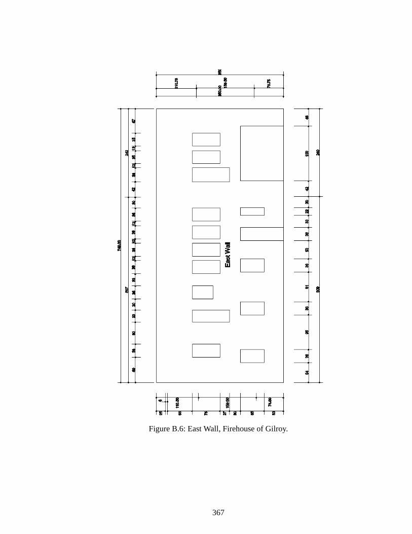
367

Figure B.6: East Wall, Firehouse of Gilroy.

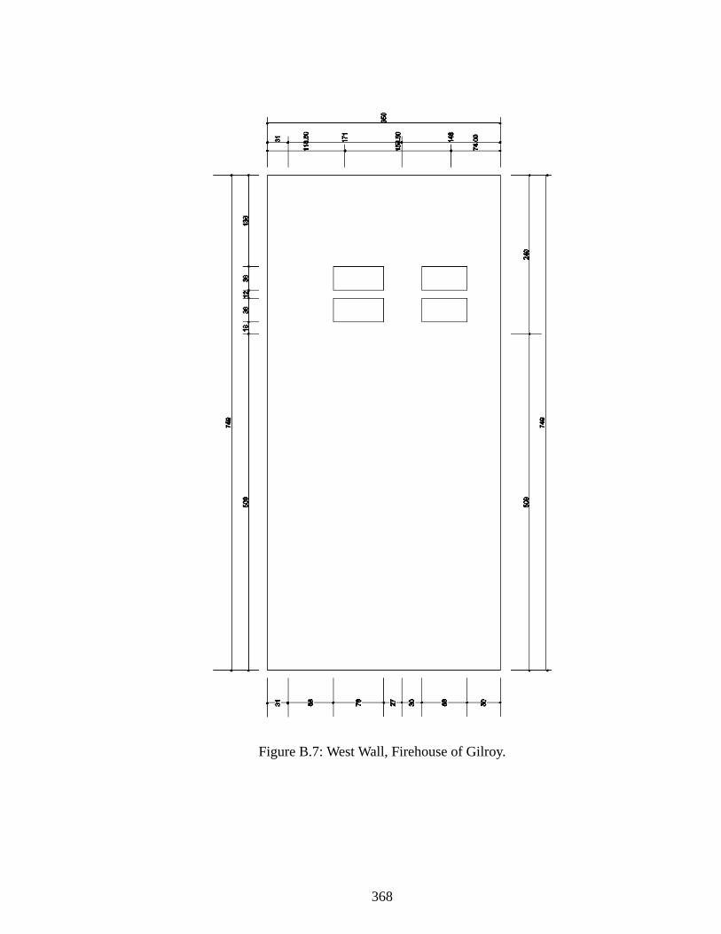
368

Figure B.7: West Wall, Firehouse of Gilroy.

369

B.2 Pier Modeling using Pier-type collapse mechanism

Figure B.8: Piers of south wall using the pier-type collapse mechanism.

Figure B.9: Piers of central wall using the pier-type collapse mechanism.

S1S3 S4

S2

S5 S7 S6S9 S11 S12 S10 S8

South Wall

C1

Center Wall

C2

C4C3

370

Figure B.10: Piers of north wall using the pier-type collapse mechanism.

Figure B.11: piers of east wall using the pier-type collapse mechanism.

N2 N3 N7N5

N1

North WallN6N4

SE1 SE2

SE8SE7

East Wall

SE3 SE4NE2NE1

NE3

NE6

SE5 SE6

SE9 SE10

SE11 SE12 SE13

SE14 NE4 NE5

371

Figure B.12: Piers of west wall using the pier-type collapse mechanism.

NW3

SW2

SW1

West Wall

NW1 NW2

NW4 NW5

NW6

372

APPENDIX C

ONE-STORY TEST BUILDING

C.1 As-built dimensions (plan)

Figure C.1: Plan of Test Building.

Figure C.2: East Wall of Test Building.

West Wall

East Wall

South Wall North WallX (Longitudinal)

Y (Transverse)

East Wall

373

Figure C.3: West Wall of Test Building.

Figure C.4: North and South Wall of Test Building.

West Wall

North andSouth Wall

374

C.2 Measured Response of Experimental Test 3 (PGA = 0.5g)

Figure C.5: Measured accelerations in the E-W direction at lifting frame (Specimen #1 Test 3) (Cohen 2001).

Figure C.6: One-second comparisons of measured accelerations in the E-W direction at lifting frame (Specimen #1 Test 3) (Cohen 2001).

-0.8-0.6-0.4-0.2

00.20.40.60.8

0 2 4 6 8 10 12 14

Time(sec)

Acc

eler

atio

n (g

) A4 A5 A6 Average

-0.8-0.6-0.4-0.2

00.20.40.60.8

4 4.2 4.4 4.6 4.8 5

Time(sec)

Acc

eler

atio

n (g

) A4 A5 A6 Average

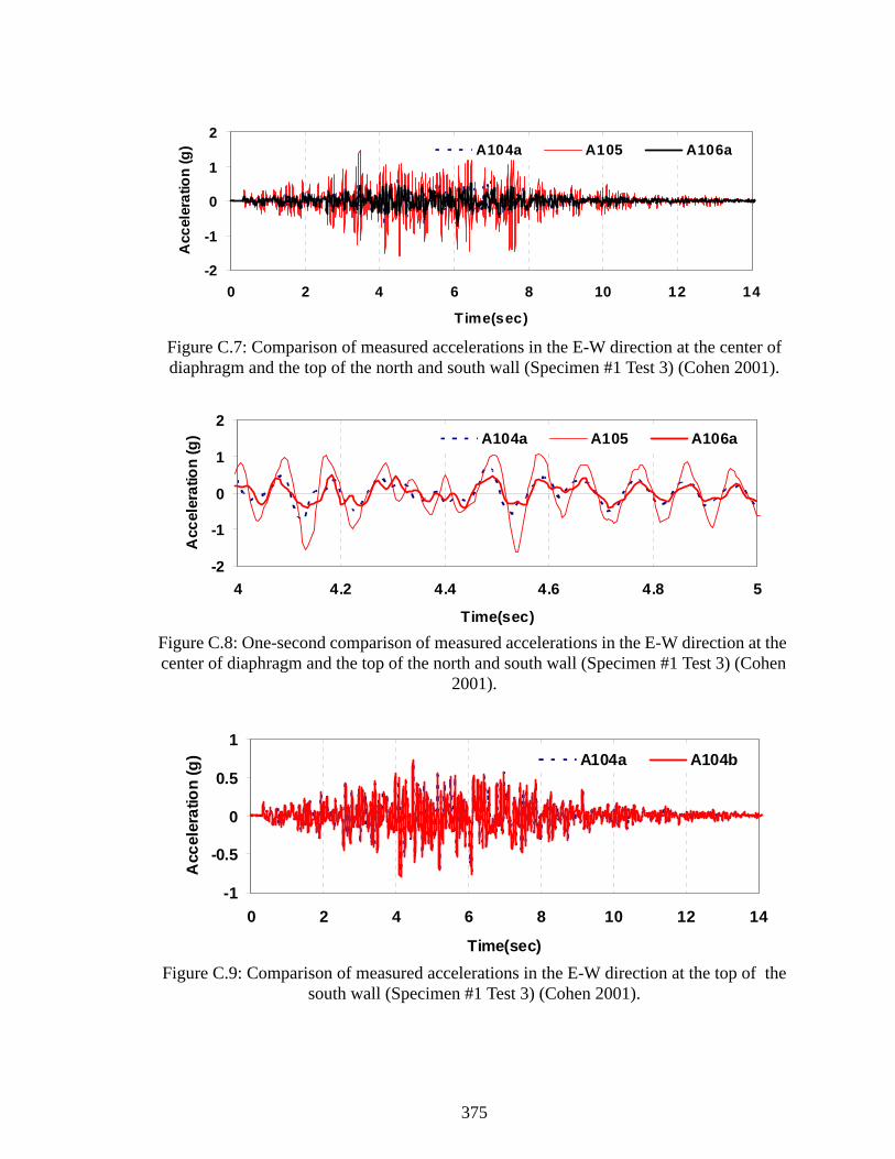
375

Figure C.7: Comparison of measured accelerations in the E-W direction at the center of diaphragm and the top of the north and south wall (Specimen #1 Test 3) (Cohen 2001).

Figure C.8: One-second comparison of measured accelerations in the E-W direction at the center of diaphragm and the top of the north and south wall (Specimen #1 Test 3) (Cohen

2001).

Figure C.9: Comparison of measured accelerations in the E-W direction at the top of the south wall (Specimen #1 Test 3) (Cohen 2001).

-2

-1

0

1

2

0 2 4 6 8 10 12 14

Time(sec)

Acc

eler

atio

n (g

) A104a A105 A106a

-2

-1

0

1

2

4 4.2 4.4 4.6 4.8 5

Time(sec)

Acc

eler

atio

n (g

) A104a A105 A106a

-1

-0.5

0

0.5

1

0 2 4 6 8 10 12 14

Time(sec)

Acc

eler

atio

n (g

) A104a A104b

376

Figure C.10: One-second comparison of measured accelerations in the E-W direction at the top of the south wall (Specimen #1 Test 3) (Cohen 2001).

Figure C.11: Measured accelerations in the E-W direction at the top of the north wall (Specimen #1 Test 3) (Cohen 2001).

Figure C.12: One-second comparison of measured accelerations in the E-W direction at the top of the north wall (Specimen #1 Test 3) (Cohen 2001).

-1

-0.5

0

0.5

1

4 4.2 4.4 4.6 4.8 5

Time(sec)

Acc

eler

atio

n (g

) A104a A104b

-0.8-0.6-0.4-0.2

00.20.40.6

0 2 4 6 8 10 12 14

Time(sec)

Acc

eler

atio

n (g

) A106a A106b

-0.8-0.6-0.4-0.2

00.20.40.6

4 4.2 4.4 4.6 4.8 5

T ime(sec)

Acc

eler

atio

n (g

) A106a A106b

377

Figure C.13: One-second comparison of measured displacements in the E-W direction (Specimen #1 Test 3) (Cohen 2001).

Figure C.14: One-second comparison of measured displacements in the E-W direction (Specimen #1 Test 3) (Cohen 2001).

Figure C.15: Comparison of measured displacements in the E-W direction at the top of the north and south wall (Specimen #1 Test 3) (Cohen 2001).

-0.15-0.1

-0.050

0.050.1

0.15

0 2 4 6 8 10 12 14

Time(sec)

Dis

plac

emen

t (in

)

RD106 RD105 RD104

-0.15-0.1

-0.050

0.050.1

0.15

4 4.2 4.4 4.6 4.8 5

Time(sec)

Dis

plac

emen

t (in

)

RD106 RD105 RD104

-0.03-0.02-0.01

00.010.020.03

0 2 4 6 8 10 12 14

Time(sec)

Dis

plac

emen

t (in

)

RD106 RD104

378

Figure C.16: One-second comparison of measured displacements in the E-W direction at the top of the north and south wall (Specimen #1 Test 3) (Cohen 2001).

C.3 Measured Response of Experimental Test 5 (PGA = 0.67g)

Figure C.17: Measured acceleration in the N-S direction at lifting frame (Specimen #1 Test 5) (Cohen 2001).

-0.03-0.02-0.01

00.010.020.03

4 4.2 4.4 4.6 4.8 5

Time(sec)

Dis

plac

emen

t (in

)

RD106 RD104

-0.1

-0.05

0

0.05

0.1

0 2 4 6 8 10 12 14Time(sec)

Acc

eler

atio

n (g

)

A1a A1b A2

379

Figure C.18: One-second comparison of measured acceleration in the N-S direction at lifting frame (Specimen #1 Test 5) (Cohen 2001).

Figure C.19: Measured acceleration in the E-W direction at lifting frame (Specimen #1 Test 5) (Cohen 2001).

Figure C.20: One-second comparison of measured acceleration in the E-W direction at lifting frame (Specimen #1 Test 5) (Cohen 2001).

-0.1

-0.05

0

0.05

0.1

4 4.2 4.4 4.6 4.8 5Time(sec)

Acc

eler

atio

n (g

) A1a A1b A2

-1

-0.5

0

0.5

1

0 2 4 6 8 10 12 14Time(sec)

Acc

eler

atio

n (g

)

A4 A5A6 Average

-1

-0.5

0

0.5

1

4 4.2 4.4 4.6 4.8 5

Time(sec)

Acc

eler

atio

n (g

) A4 A5 A6 Average

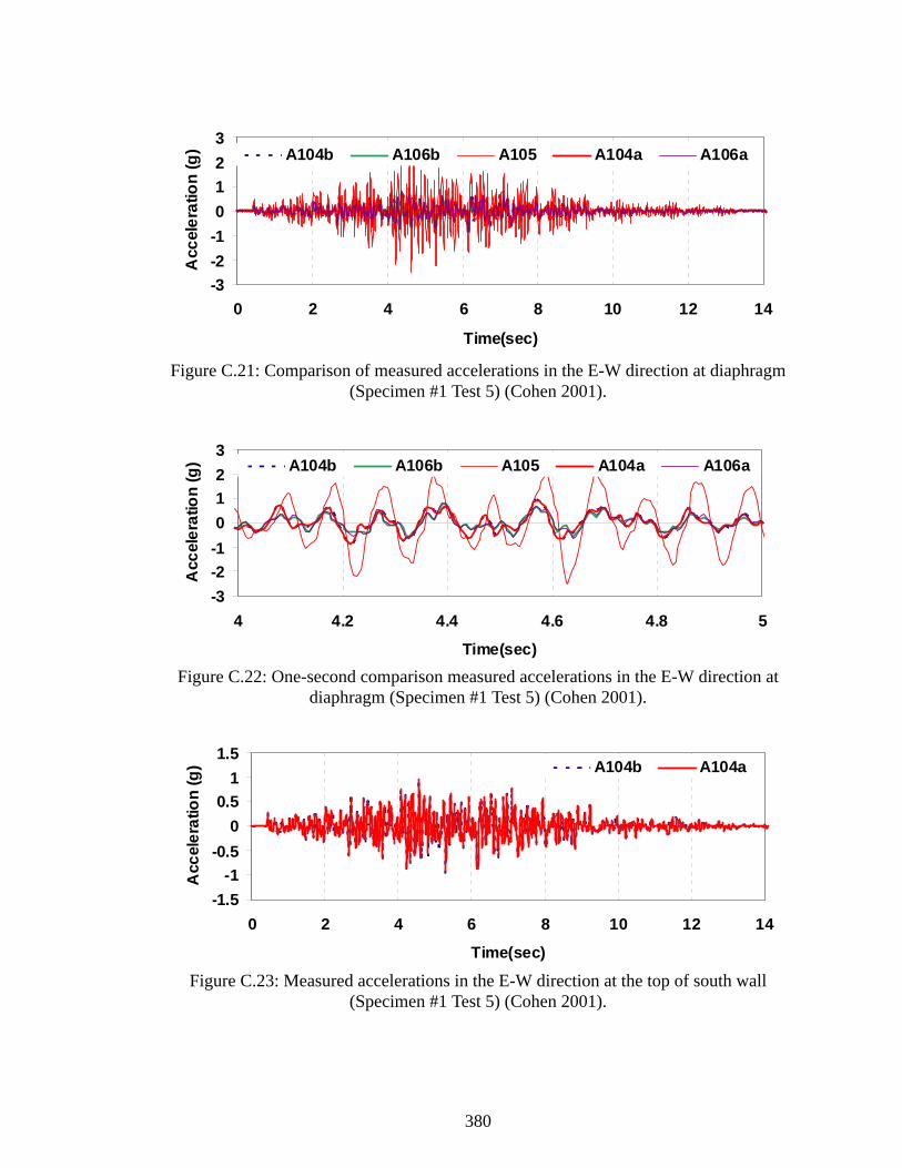
380

Figure C.21: Comparison of measured accelerations in the E-W direction at diaphragm (Specimen #1 Test 5) (Cohen 2001).

Figure C.22: One-second comparison measured accelerations in the E-W direction at diaphragm (Specimen #1 Test 5) (Cohen 2001).

Figure C.23: Measured accelerations in the E-W direction at the top of south wall (Specimen #1 Test 5) (Cohen 2001).

-3-2-10123

0 2 4 6 8 10 12 14

Time(sec)

Acc

eler

atio

n (g

) A104b A106b A105 A104a A106a

-3-2-10123

4 4.2 4.4 4.6 4.8 5

Time(sec)

Acc

eler

atio

n (g

) A104b A106b A105 A104a A106a

-1.5-1

-0.50

0.51

1.5

0 2 4 6 8 10 12 14

Time(sec)

Acc

eler

atio

n (g

) A104b A104a

381

Figure C.24: One-second comparison of measured accelerations in the E-W direction at the top of south wall (Specimen #1 Test 5) (Cohen 2001).

Figure C.25: Measured accelerations in the E-W direction at the top of north wall (Specimen #1 Test 5) (Cohen 2001).

Figure C.26: One-second comparison of measured accelerations in the E-W direction at the top of north wall (Specimen #1 Test 5) (Cohen 2001).

-1.5-1

-0.50

0.51

1.5

4 4.2 4.4 4.6 4.8 5

Time(sec)

Acc

eler

atio

n (g

) A104b A104a

-1

-0.5

0

0.5

1

0 2 4 6 8 10 12 14

Time(sec)

Acc

eler

atio

n (g

) A106b A106a

-1

-0.5

0

0.5

1

4 4.2 4.4 4.6 4.8 5Time(sec)

Acc

eler

atio

n (g

) A106b A106a

382

Figure C.27: Measured displacements in the E-W direction (Specimen #1 Test 5) (Cohen 2001).

Figure C.28: One-second comparison of measured displacements in the E-W direction (Specimen #1 Test 5) (Cohen 2001).

Figure C.29: Measured displacements in the E-W direction at the top of the north and south wall (Specimen #1 Test 5) (Cohen 2001).

-0.3-0.2-0.1

00.10.20.3

0 2 4 6 8 10 12 14

Time(sec)

Dis

plac

emen

t (in

)

D104 D105 D106

-0.3-0.2-0.1

00.10.20.3

4 4.2 4.4 4.6 4.8 5

Time(sec)

Dis

plac

emen

t (in

) D104 D105 D106

-0.04

-0.02

0

0.02

0.04

0 2 4 6 8 10 12 14

Time(sec)

Dis

plac

emen

t (in

)

D104 D106

383

Figure C.30: One-second comparison of measured displacements in the E-W direction at the top of the north and south wall (Specimen #1 Test 5) (Cohen 2001).

C.4 Measured Response of Experimental Test 9 (PGA = 1.0 g)

Figure C.31: Measured accelerations in the E-W direction at lifting frame (Specimen #1 Test 9) (Cohen 2001).

-0.04

-0.02

0

0.02

0.04

4 4.2 4.4 4.6 4.8 5

Time(sec)

Dis

plac

emen

t (in

) D104 D106

-1.2

-0.6

0

0.6

1.2

0 2 4 6 8 10 12 14

Time(sec)

Acc

eler

atio

n (g

) A4 A5 A6 Average

384

Figure C.32: One-second comparisons of measured accelerations in the E-W direction at lifting frame (Specimen #1 Test 9) (Cohen 2001).

Figure C.33: Comparison of measured accelerations in the E-W direction at the center of diaphragm and the top of the north and south wall (Specimen #1 Test 9) (Cohen 2001).

Figure C.34: One-second comparison of measured accelerations in the E-W direction at the center of diaphragm and the top of the north and south wall (Specimen #1 Test 9)

(Cohen 2001).

-1.2

-0.6

0

0.6

1.2

4 4.2 4.4 4.6 4.8 5

Time(sec)

Acce

lera

tion

(g) A4 A5 A6 Average

-4-3-2-10123

0 2 4 6 8 10 12 14

Time(sec)

Acc

eler

atio

n (g

)

A104a A105 A106a

-4-3-2-10123

4 4.2 4.4 4.6 4.8 5

Time(sec)

Acc

eler

atio

n (g

) A104a A105 A106a

385

Figure C.35: Comparison of measured accelerations in the E-W direction at the top of north and south wall (Specimen #1 Test 9) (Cohen 2001).

Figure C.36: One-second comparison of measured accelerations in the E-W direction at the top of north and south wall (Specimen #1 Test 9) (Cohen 2001).

Figure C.37: Comparison of measured accelerations in the E-W direction at the top of south wall (Specimen #1 Test 9) (Cohen 2001).

-1.5-1

-0.50

0.51

1.5

0 2 4 6 8 10 12 14

Time(sec)

Acc

eler

atio

n (g

) A104a A106a

-1.5-1

-0.50

0.51

1.5

4 4.2 4.4 4.6 4.8 5

Time(sec)

Acc

eler

atio

n (g

) A104a A106a

-1.5-1

-0.50

0.51

1.5

0 2 4 6 8 10 12 14

Time(sec)

Acc

eler

atio

n (g

) A104a A104b

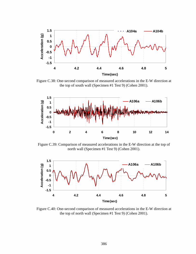
386

Figure C.38: One-second comparison of measured accelerations in the E-W direction at the top of south wall (Specimen #1 Test 9) (Cohen 2001).

Figure C.39: Comparison of measured accelerations in the E-W direction at the top of north wall (Specimen #1 Test 9) (Cohen 2001).

Figure C.40: One-second comparison of measured accelerations in the E-W direction at the top of north wall (Specimen #1 Test 9) (Cohen 2001).

-1.5-1

-0.50

0.51

1.5

4 4.2 4.4 4.6 4.8 5

Time(sec)

Acc

eler

atio

n (g

) A104a A104b

-1.5-1

-0.50

0.51

1.5

0 2 4 6 8 10 12 14

Time(sec)

Acc

eler

atio

n (g

) A106a A106b

-1.5-1

-0.50

0.51

1.5

4 4.2 4.4 4.6 4.8 5

Time(sec)

Acc

eler

atio

n (g

) A106a A106b

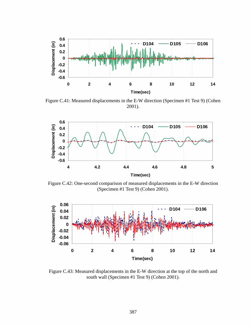
387

Figure C.41: Measured displacements in the E-W direction (Specimen #1 Test 9) (Cohen 2001).

Figure C.42: One-second comparison of measured displacements in the E-W direction (Specimen #1 Test 9) (Cohen 2001).

Figure C.43: Measured displacements in the E-W direction at the top of the north and south wall (Specimen #1 Test 9) (Cohen 2001).

-0.6-0.4-0.2

00.20.40.6

0 2 4 6 8 10 12 14

Time(sec)

Dis

plac

emen

t (in

) D104 D105 D106

-0.6-0.4-0.2

00.20.40.6

4 4.2 4.4 4.6 4.8 5

Time(sec)

Dis

plac

emen

t (in

) D104 D105 D106

-0.06-0.04-0.02

00.020.040.06

0 2 4 6 8 10 12 14

Time(sec)

Dis

plac

emen

t (in

)

D104 D106

388

Figure C.44: One-second comparison of measured displacements in the E-W direction at the top of the north and south wall (Specimen #1 Test 9)(Cohen 2001).

C.5 Comparison of Measured and Calculated Response using PGA = 0.5 g

Figure C.45: Comparison of acceleration in the E-W direction at the top of south wall (PGA =0.5g).

-0.06-0.04-0.02

00.020.040.06

4 4.2 4.4 4.6 4.8 5

Time(sec)

Dis

plac

emen

t (in

)D104 D106

-1.0

-0.5

0.0

0.5

1.0

0 2 4 6 8Time (sec)

Acc

eler

atio

n (g

) Measured Calculated

389

Figure C.46: Two-second comparison of acceleration in the E-W direction at the top of south wall (PGA =0.5g).

Figure C.47: Comparison of acceleration in the E-W direction at the top of north wall (PGA =0.5g).

Figure C.48: Two-second comparison of acceleration in the E-W direction at the top of north wall (PGA =0.5g).

-1.0

-0.5

0.0

0.5

1.0

4 4.5 5 5.5 6Time (sec)

Acc

eler

atio

n (g

) Measured Calculated

-1.0

-0.5

0.0

0.5

1.0

0 2 4 6 8Time (sec)

Acc

eler

atio

n (g

) Measured Calculated

-1.0

-0.5

0.0

0.5

1.0

4 4.5 5 5.5 6Time (sec)

Acc

eler

atio

n (g

) Measured Calculated

390

Figure C.49: Comparison of displacement in the E-W direction at the top of south wall (PGA =0.5g).

Figure C.50: Two-second comparison of displacement in the E-W direction at the top of south wall (PGA =0.5g).

Figure C.51: Comparison of displacement in the E-W direction at the top of north wall (PGA =0.5g).

-0.03-0.02-0.010.000.010.020.03

0 2 4 6 8Time (sec)

Dis

plac

emen

t (in

) Measured Calculated

-0.03-0.02-0.010.000.010.020.03

4 4.5 5 5.5 6Time (sec)

Dis

plac

emen

t (in

) Measured Calculated

-0.03-0.02-0.010.000.010.020.03

0 2 4 6 8Time (sec)

Dis

plac

emen

t (in

) Measured Calculated

391

Figure C.52: Two-second comparison of displacement in the E-W direction at the top of north wall (PGA =0.5g).

C.6 Comparison of Measured and Calculated Response using PGA = 0.67 g

Figure C.53: Comparison of acceleration in the E-W direction at the top of south wall (PGA =0.67g).

-0.03-0.02-0.010.000.010.020.03

4 4.5 5 5.5 6Time (sec)

Dis

plac

emen

t (in

) Measured Calculated

-1.0

-0.5

0.0

0.5

1.0

0 2 4 6 8Time (sec)

Acc

eler

atio

n (g

) Measured Calculated

392

Figure C.54: Two-second comparison of acceleration in the E-W direction at the top of south wall (PGA =0. 67g).

Figure C.55: Comparison of acceleration in the E-W direction at the top of north wall (PGA =0. 67g).

Figure C.56: Two-second comparison of acceleration in the E-W direction at the top of north wall (PGA =0.67g).

-1.0

-0.5

0.0

0.5

1.0

4 4.5 5 5.5 6Time (sec)

Acc

eler

atio

n (g

) Measured Calculated

-1.0

-0.5

0.0

0.5

1.0

0 2 4 6 8Time (sec)

Acc

eler

atio

n (g

) Measured Calculated

-1.0

-0.5

0.0

0.5

1.0

4 4.5 5 5.5 6Time (sec)

Acc

eler

atio

n (g

) Measured Calculated

393

Figure C.57: Comparison of displacement in the E-W direction at the top of south wall (PGA =0. 67g).

Figure C.58: Two-second comparison of displacement in the E-W direction at the top of south wall (PGA =0. 67g).

Figure C.59: Comparison of displacement in the E-W direction at the top of north wall (PGA =0. 67g).

-0.03-0.02-0.010.000.010.020.03

0 2 4 6 8Time (sec)

Dis

plac

emen

t (in

) Measured Calculated

-0.03-0.02-0.010.000.010.020.03

4 4.5 5 5.5 6Time (sec)

Dis

plac

emen

t (in

) Measured Calculated

-0.03-0.02-0.010.000.010.020.03

0 2 4 6 8Time (sec)

Dis

plac

emen

t (in

) Measured Calculated

394

Figure C.60: Two-second comparison of displacement in the E-W direction at the top of north wall (PGA =0. 67g).

C.7 Comparison of Measured and Calculated Response using PGA = 1.0 g

Figure C.61: Comparison of acceleration in the E-W direction at the top of south wall (PGA =1.0g).

-0.03-0.02-0.010.000.010.020.03

4 4.5 5 5.5 6Time (sec)

Dis

plac

emen

t (in

) Measured Calculated

-2.0

-1.0

0.0

1.0

2.0

0 2 4 6 8Time (sec)

Acc

eler

atio

n (g

) Measured Calculated

395

Figure C.62: Two-second comparison of acceleration in the E-W direction at the top of south wall (PGA = 1.0g).

Figure C.63: Comparison of acceleration in the E-W direction at the top of north wall (PGA = 1.0g).

Figure C.64: Two-second comparison of acceleration in the E-W direction at the top of north wall (PGA = 1.0g).

-2.0

-1.0

0.0

1.0

2.0

4 4.5 5 5.5 6Time (sec)

Acc

eler

atio

n (g

) Measured Calculated

-2.0

-1.0

0.0

1.0

2.0

0 2 4 6 8Time (sec)

Acc

eler

atio

n (g

) Measured Calculated

-2.0

-1.0

0.0

1.0

2.0

4 4.5 5 5.5 6Time (sec)

Acc

eler

atio

n (g

) Measured Calculated

396

Figure C.65: Comparison of displacement in the E-W direction at the top of south wall (PGA = 1.0g).

Figure C.66: Two-second comparison of displacement in the E-W direction at the top of south wall (PGA = 1.0g).

Figure C.67: Comparison of displacement in the E-W direction at the top of north wall (PGA = 1.0g).

-0.06-0.04-0.020.000.020.040.06

0 2 4 6 8Time (sec)

Dis

plac

emen

t (in

) Measured Calculated

-0.06-0.04-0.020.000.020.040.06

4 4.5 5 5.5 6Time (sec)

Dis

plac

emen

t (in

) Measured Calculated

-0.06-0.04-0.020.000.020.040.06

0 2 4 6 8Time (sec)

Dis

plac

emen

t (in

) Measured Calculated

397

Figure C.68: Two-second comparison of displacement in the E-W direction at the top of north wall (PGA = 1.0g).

-0.06-0.04-0.020.000.020.040.06

4 4.5 5 5.5 6Time (sec)

Dis

plac

emen

t (in

) Measured Calculated

398

APPENDIX D

ANALYSIS SYSTEM

D.1 Overview of ABAQUS user element library

The ABAQUS finite element system has been used as a general-purpose finite ele-

ment program. This system is operational on Windows NT and UNIX systems. ABAQUS/

Standard is a versatile analysis tool with a large number of element libraries that allows

analysis of complex structural problems. And it has an interface that allows users to imple-

ment linear and nonlinear finite elements. User subroutines that are available in ABAQUS

gives an extremely powerful and flexible tool for analysis. These subroutines (UEL,

UMAT, UMATHT, UMATHT, UGENS, and so on) are typically written as FORTRAN

code and are used to extend the capabilities of ABAQUS. UEL subroutine is used to

make User-defined elements which are invoked in the same way as native ABAQUS ele-

ments (ABAQUS 1998).

The wall and diaphragm elements discussed in previous chapters were imple-

mented in a user subroutine UEL. The interface makes it possible to define any element of

arbitrary complexity. Multiple user elements can be implemented in a single UEL routine

and can be utilized together.

The software developed in this project, as shown in Fig. D.1, can model three-

dimensional Low-Rise buildings with flexible floor diaphragms. Currently, one nonlinear

wall and one diaphragm element are included in the code. A schematic model of a repre-

sentative low-rise building is shown in Fig. D.2. The nonlinear wall element is designed

to represent a bearing wall under shear loadings. Diagonal shear, bed joint sliding, rock-

ing and toe crushing behavior of shear walls are considered in the wall element.

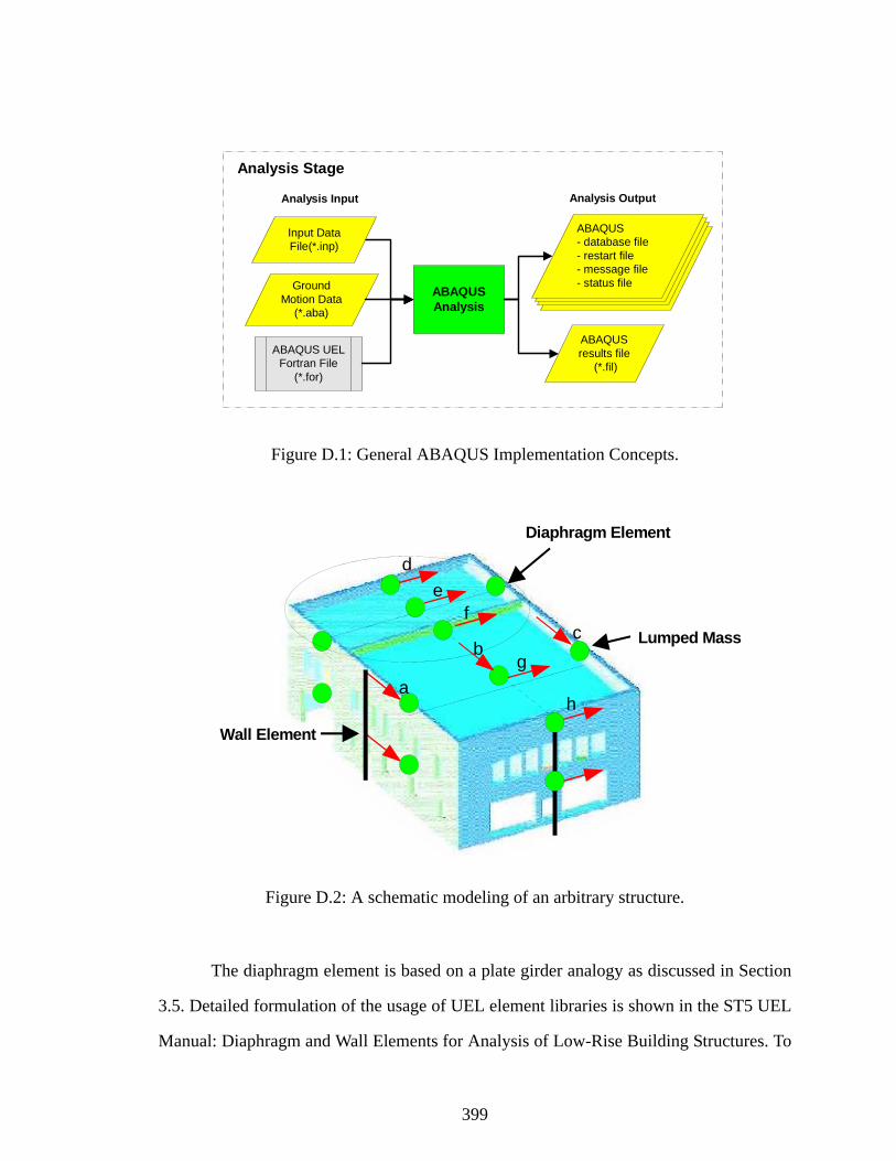
399

Figure D.1: General ABAQUS Implementation Concepts.

Figure D.2: A schematic modeling of an arbitrary structure.

The diaphragm element is based on a plate girder analogy as discussed in Section

3.5. Detailed formulation of the usage of UEL element libraries is shown in the ST5 UEL

Manual: Diaphragm and Wall Elements for Analysis of Low-Rise Building Structures. To

Analysis Stage

Analysis OutputAnalysis Input

GroundMotion Data

(*.aba)

ABAQUSAnalysis

ABAQUS UELFortran File

(*.for)

ABAQUSresults file

(*.fil)

ABAQUS- database file- restart file- message file- status file

Input DataFile(*.inp)

a

bc

de

f

g

h

Diaphragm Element

Wall Element

Lumped Mass

400

use the manual, it is assumed that reader is familiar with the nonlinear time history analy-

sis and the format of ABAQUS input data files.

D.1.1 Types of analysis

The software developed in this project has the capability of the static and dynamic

analysis (Nonlinear Time history analysis) with any combination of several static or

dynamic loading conditions. For the static analysis, there are two types of analysis: linear

and nonlinear static analysis. Linear static analysis involves the specification of load cases

and appropriate boundary conditions. In most nonlinear analyses the loading variations

over the step follow a prescribed displacement or force history.

For the nonlinear time history analysis, the general direct-integration method pro-

vided in ABAQUS/Standard, called the Hilber-Hughes-Taylor operator, is used (Hilber et

al, 1978). The integration method is an extension of the trapezoidal rule. A set of simul-

taneous nonlinear dynamic equilibrium equations must be solved at each time increment.

ABAQUS/Standard generally uses Newton’s method to solve the nonlinear equilibrium

equations. The principal advantage of the Hilber-Hughes-Taylor operator is uncondition-

ally stable for linear systems.

Damping.

ABAQUS is using an artificial damping, which is purely numerical. The ALPHA

parameter introduces damping that grows with the ratio of the time increment to the period

of vibration of a mode. In this project, the Newmark -Method is used. Since the New-

mark -Method, which gives no artificial damping, is exactly the trapezoidal rule, the

ALPHA parameter in ABAQUS is set to zero.

β

β

401

Baseline correction.

For a dynamic analysis, when an amplitude definition, such as earthquake acceler-

ation history, is used, the integration of the acceleration record through time may result in

a relatively large displacement at the end of the event. This behavior typically occurs

because of instrumentation errors or a sampling frequency that is not sufficient to capture

the actual acceleration history. It is possible to compensate for it by using "baseline correc-

tion."

ABAQUS allows an acceleration history to be modified to minimize the overall

drift of the displacement obtained from the time integration of the given acceleration. The

use of more correction intervals provides tighter control over any “drift” in the displace-

ment at the expense of more modification of the given acceleration trace. In either case,

the modification begins with the start of the amplitude variation and with the assumption

that the initial velocity at that time is zero.

Absolute and Relative Response.

Research engineers use two types of energy equations to study single-degree-of-

freedom systems subject to earthquake induced ground motions. The first method uses an

absolute energy formulation; the second method uses a relative energy formulation. While

the relative energy formulation has been used in the majority of previous investigations.

The reference study shows that the absolute energy equation is physically more meaning-

ful (Chia-Ming Uang et al, 1990).

The use of an ‘absolute’ energy equation rather that a ‘relative’ energy equation

has the advantage that the physical energy input is reflected. For certain types of earth-

quake ground motion, the absolute input energy spectra are sensitive to the variation of

ductility ratio. Except for the highly harmonic earthquakes, the absolute input energy

spectra for a constant ductility ratio can be predicted reliably by the elastic input energy

spectra using Iwan’s procedure which takes into consideration the effect of increasing

402

damping ratio and natural period. For steel dual systems of medium rise buildings it is

possible to estimate with sufficient accuracy the input energy for a multi-story building

structure from the absolute input energy spectra for a SDOF system and the fundamental

period of the multi-story structure.

The first objective of this paper is to analyze the physical meaning of two energy

equations that are derived and used in the literature. The second objective is to use these

two definitions to construct inelastic input energy spectra for a SDOF system.

D.1.2 ABAQUS user element definitions

Defining a User Element

Before a UEL routine can be written, the following key characteristics of the element must

be defined: The number of nodes on the element, the number of coordinates present at

each node and the degrees of freedom active at each node. In addition, the following prop-

erties must be determined: 1) the number of element properties need to be defined external

to the UEL for each element type, and 2) the number of solution-dependent state variables

(SDVs) must be stored for each element type. These items need not be determined imme-

diately: they can be added easily after the basic UEL subroutine is completed.

User Elements

In this project, three wall elements and two diaphragm elements are developed.

These elements are defined as follows:

1. Combined Kinematic and Isotropic Hardening Wall Element

2. Rocking Wall Element

3. Park’s Three Parameter Wall Element

403

4. Combined Kinematic and Isotropic Hardening Diaphragm Element

5. Park’s Three Parameter Diaphragm Element

The diaphragm elements can be categorized into two types. The first type consid-

ers the effect of the bending and shear of the diaphragm at the same time, and the second

type accounts for only shear of the web.

D.1.3 UEL Interface (Input file variables)

A user element is defined with the *USER ELEMENT option. This option must

appear in the input file before the user element is invoked with the *ELEMENT option.

The syntax for interfacing to UEL is as follows:

* USER ELEMENT TYPE=Un , NODES= , COORDINATES= ,

PROPERTIES= , I PROPERTIES= , VARIABLES=, UNSYMM

Data line(s)

*ELEMENT,TYPE=Un, ELSET=UEL

Data line(s)

*UEL PROPERTY,ELSET=UEL

Data line(s)

*USER SUBROUTINE, (INPUT=filename)

Example)

*UEL PROPERTY,ELSET=UTRUSS

1.0, 10000000., 0.2, 10., 100000., 20000., 0.0

AREA, E, NU (poisson's ratio), RHO (material density), Et (inelastic tangent modulus of matl), Fyi,

(initial yield stress of matl) , AISO (Isotropic hardening fraction)

404

Table D.1: Outline UEL Input Variables.

D.2 Definition of earthquake accelerations

As shown in Fig. D.1, a dynamic analysis in ABAQUS is defined by two input file:

model data and history data. To define the earthquake acceleration in model data file, the

*amplitude option is used.

Example)

*amplitude, definition=tabular, value=relative, input=ch3m2a.acc, name=earth

The earthquake acceleration loading is prescribed as a function of time, so called

“Amplitude curves”. This feature is used to prescribe a seismic event. The INPUT option

is used to specify an external file that contains history definition data. When the option is

encountered, ABAQUS will immediately process the input data within the file specified

by the INPUT parameter. When the end-of-file is reached, ABAQUS returns to processing

the original file.

VARIABLES NOTE

TYPE (User defined) element type of the form Un, where n is a number

NODES Number of nodes on the element

COORDINATES Maximum number of coordinates at any node

PROPERTIES Number of floating point properties

I-PROPERTIES Number of integer properties

VARIABLES Number of SDVs

UNSYMM Flag to indicate that the Jacobian is non symmetric

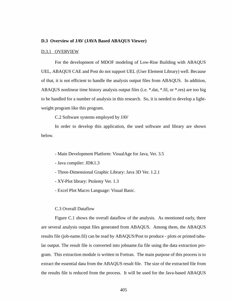
405

D.3 Overview of JAV (JAVA Based ABAQUS Viewer)

D.3.1 OVERVIEW

For the development of MDOF modeling of Low-Rise Building with ABAQUS

UEL, ABAQUS CAE and Post do not support UEL (User Element Library) well. Because

of that, it is not efficient to handle the analysis output files from ABAQUS. In addition,

ABAQUS nonlinear time history analysis output files (i.e. *.dat, *.fil, or *.res) are too big

to be handled for a number of analysis in this research. So, it is needed to develop a light-

weight program like this program.

C.2 Software systems employed by JAV

In order to develop this application, the used software and library are shown

below.

- Main Development Platform: VisualAge for Java, Ver. 3.5

- Java compiler: JDK1.3

- Three-Dimensional Graphic Library: Java 3D Ver. 1.2.1

- XY-Plot library: Ptolemy Ver. 1.3

- Excel Plot Macro Language: Visual Basic.

C.3 Overall Dataflow

Figure C.1 shows the overall dataflow of the analysis. As mentioned early, there

are several analysis output files generated from ABAQUS. Among them, the ABAQUS

results file (job-name.fil) can be read by ABAQUS/Post to produce - plots or printed tabu-

lar output. The result file is converted into jobname.fia file using the data extraction pro-

gram. This extraction module is written in Fortran. The main purpose of this process is to

extract the essential data from the ABAQUS result file. The size of the extracted file from

the results file is reduced from the process. It will be used for the Java-based ABAQUS

406

viewer (JAV) program to handle the analysis results. In JAV program there are several

capabilities: X-Y plotting of nodal relative and absolute displacement, velocity, and accel-

eration history; X-Y plot of wall element force and displacement history; and animation of

the whole structure. The hardcopy of example snaps captured from the screen are shown

in next section.

Figure D.3: Overall Dataflow.

Analysis Stage

Post Process Stage

Analysis OutputAnalysis Input

GroundMotion Data

(*.aba)

ABAQUSAnalysis

ABAQUS UELFortran File

(*.for)

ABAQUSresults file

(*.fil)

ABAQUS- database file- restart file- message file- status file

Data ExtractProgram(Post.for)

Extracted File (*.fia)

Java-BasedABAQUS Viewer

(JAV Ver 1.0)

Summary ofAnalysis Result

(*.dat)

MS Excel File forAnalysis Results

(*.xls)

ExcelLoader(*.bas)

Graphic OutputPIctures andAnimation file

: Input or Out put Data File

: Predefined External Module

: Main Process

Input DataFile(*.inp)

407

D.3.2 Main Program

The 3D graph of this program is constructed by a Java 3D program. The mouse

utility behavior package contains behavior classes in which the mouse is used as input for

interaction with visual objects. Included are classes for translating (moving in a plane par-

allel to the image plate), zooming (moving forward and back), and rotating visual objects

in response to mouse movements

Figure D.4: Main Program.

Model Drawing Panel Text Display Consol

Time History Results Icons

Model and Element InformaioIcons Model Number Text

Control Box

408

REFERENCES

ABK (1981a). “Methodology for mitigation of seismic hazards in existing unreinforcedmasonry buildings: Categorization of buildings.” ABK Tech. Rep. 01, ABK, A JointVenture, El Segundo, Calif.

ABK (1981b). “Methodology for mitigation of seismic hazards in existing unreinforcedmasonry buildings: Diaphragm testing.” ABK Tech. Rep. 03, ABK, A Joint Venture,El Segundo, Calif.

ABK (1984). “Methodology for mitigation of seismic hazards in existing unreinforcedmasonry buildings: Diaphragms: the methodology.” ABK Tech. Rep. 08, ABK, AJoint Venture, El Segundo, Calif.

Abrams, D. P. (1992). “Strength and behavior of unreinforced masonry elements.” Proc.10th World Conf. on Earthquake Engineering, Madrid, Spain, Vol. 10, 3475-3480.

Abrams, D. P. (2001). “Performance-based engineering concepts for unreinforcedmasonry building structures.” Progress in Structural Engineering and Materials, Vol.3, Issue 1, pp. 48-56.

Adhikari, S. and Woodhouse, J. (2001) “Identification of Damping: Part 1, Viscous Damp-ing.” Journal of Sound and Vibration, 243(1), 43-61

Ali, S. S. and Page, A. W. (1988). “Finite element model for masonry subjected to concen-trated loads.” J. Struct. Engrg., ASCE, 114(8), 1761 - 1784.

Anand, S.C. and Yalamanchili, K.K. (1996). “ Three-dimensional failure analysis of com-posite masonry walls.” J. Struct. Engrg., ASCE, 122(9), 1031-1039

APA (1997a). “DIAPHRAGMS AND SHEAR WALLS.” American Plywood Associa-tion, Tacoma, Wash.

APA (1997b). “Plywood Design Specification” American Plywood Association, Tacoma,Wash.

Argyris, J. H. et al. (1978). “Finite Element Method - the Natural Approach.” ComputMethods in Applied Mechanics and Engineering, Vols. 17/18, 1-106

409

ASCE (2000a). “FEMA 356: Prestandard and Commentary for the Seismic Rehabilitationof Buildings.” Publication No. 356, prepared by the American Society of Civil Engi-neers, funded by the Federal Emergency Management Agency,American Society ofCivil Engineers, Washington, DC.

ASCE (2000b). “FEMA 357: Global Topics Report on The Prestandard and Commentaryfor The Seismic Rehabilitation of Buildings.” Publication No. 357, prepared by theAmerican Society of Civil Engineers, funded by the Federal Emergency Manage-ment Agency,American Society of Civil Engineers, Washington, DC

ATC (1981). “Guidelines for the Design of Horizontal Wood Diaphragms.” Applied Tech-nology Council, ATC 7, Washington, D.C.

ATC (1987). “Tentative Provisions for the Development of Seismic Regulations for Build-ings.” ATC 3-06, NBS Special Publication 510, Washington D.C.

ATC (1998). “FEMA 306: Evaluation of Earthquake Damaged Concrete and Masonrywall buildings-Basic Procedures Manual.” Applied Technology Council, ATC-43Project, Redwood City, CA.

Bathe, K., (1996). “ Finite Element Procedures”, Prentice Hall, Englewood Cliffs, NewJersey.

Benedetti, D., and Castellani, A. (1980). “Dynamic versus static behavior of a masonrystructure under lateral loads.” Eng. Struct, Vol. 2, 163-170

Button, M. R., Kelly, T. E., and Jones, L. R. (1984). “The influence of diaphragm flexibil-ity on the seismic response of buildings,” Proc. 8th World Conf. on EarthquakeEngineering, Vol. 4, San Francisco, CA, 759-766.

Calvi, G. M. and Kingsley, G. R. (1995). “Displacement-based seismic design of multi-degree of-freedom bridge structures.” Earthquake Engineering and StructuralDynamics, Vol. 24, 1247-1266

Carney, J.M. (1975). “Bibliography on wood and plywood diaphragms.” Journal of theStructural Division, ASCE, 101(ST11), 2433 - 2436.

Chopra, A. K. (1995). “Dynamics of Structures – Theory and Applications To EarthquakeEngineering.” Prentice Hall, Englewood Cliffs, New Jersey

Clough, R.W. and Penzien, J. (1993) “ Dynamics of Structures - 2nd Ed.” McGraw-HillInc., New York.

Cohen, G.L. (2001). “Seismic Response of Low-Rise Masonry Buildings with FlexibleRoof Diaphragms.” M.S Thesis, University of Texas, Austin.

410

Cohen, G.L. and Klingner, R. E. (2001a). “Seismic Behavior and Evaluation of FlexibleRoof Diaphragms.” US Army CERL report, University of Texas, Austin.

Cohen, G.L. and Klingner, R. E. (2001b), personal communication

Cohen, G.L. (2002), personal communication.

Coil, J. (1999), personal communication.

Cook, R. D., Malkus, D. S., and Plesha M. E. (1989). “Concepts and Applications ofFinite Element Analysis - 3rd Ed.” John Wiley & Sons, New York

Costley, A. C., Abrams, D.P., and Calvi, G. M. (1994). “Shaking-Table Testing of AnUnreinforced Brick Masonry Building.” Proc., Fifth U.S. National Conference onEarthquake Engrg.,Vol. I, EERI, Chicago, Ill, 127-146.

Costley, A. C. and Abrams, D.P. (1996). “Dynamic response of unreinforced masonrybuildings with flexible diaphragms.” Tech. Rep. NCEER-96-0001, Nat. Ctr. forEarthquake Engrg. Res., Buffalo, N.Y.

Davies, J. M. (1976). “Simplified diaphragm analysis.” J. Struct. Div., ASCE, 103(11),2093-2109

DenHartog, J.P. (1985) Mechanical Vibrations - 4th Edition, Dover

Dolce, M., Lorusso, V.D., and Masi, A. (1994). “Seismic response of building structureswith flexible inelastic diaphragm.” Struct. Design Tall Build., John Wiley & Sons,Ltd, 3, 87-106

Easterling, R.G.(1999). “A Framework for Model Validation.” Report No: SAND99-0301C, Sandia National Laboratories, Albuquerque, NM, and Livermore, CA.

Easterling, W.S. and Porter, M.L. (1994a). “Steel-Deck-Reinforced Concrete Diaphragm.I.” J. Struct. Engrg., ASCE, 120(2), 560 - 576.

Easterling, W.S. and Porter, M.L. (1994b). “Steel-Deck-Reinforced Concrete Diaphragm.II.” J. Struct. Engrg., ASCE, 120(2), 577 - 596.

Erbay, O. O. and Abrams, D.P.(2002). “Seismic rehabilitation of unreinforced masonryshear walls.” Proc. Seventh U.S. National Conference on Earthquake Engrg., EERI,Boston, Massachusetts.

CEN (1995). “Eurocode 6: Design of masonry structures, Part 1-1: General rules forbuildings. Rules for reinforced and unreinforced masonry.” European Committeefor Standardization, ENV 1996-1-1, Brussels

411

Ewing, R. D., El-Mustapha, A. M., and Kariostis, J. C. (1987). “FEM / I: A finite elementcomputer program for the nonlinear static analysis of reinforced masonry buildingcomponents.” EKEH (Ewing / Kariostis / Englekirk & Hart Ewing & Associates),CA

Falk, R. H. and Itani, R. Y. (1987). “Dynamic Characteristics of wood and gypsum dia-phragms.” J. Struct. Engrg., ASCE, 113(6), 1357-1370.

Falk, R. H. and Itani, R. Y. (1989). “Finite element modeling of wood diaphragms.” J.Struct. Engrg., ASCE, 115(3), 543 - 559.

FEMA (1992a). “Evaluation of unreinforced masonry bearing wall buildings.” NEHRPhandbook for the seismic evaluation of existing buildings; Federal EmergencyMgmt. Agency, Rep. No. 178, Build. Seismic Safety Council, Washington, D.C.

FEMA (1992b). “NEHRP Handbook for the Seismic Evaluation of Existing Buildings.”Federal Emergency Mgmt. Agency, Rep. No. 178, Washington, D.C.

FEMA (1997a). “NEHRP Guidelines for the Seismic Rehabilitation of Building.” FederalEmergency Mgmt. Agency, Rep. No. 273, Build. Seismic Safety Council, Washing-ton, D.C.

FEMA (1997a). “NEHRP Commentary on the Guidelines for the Seismic Rehabilitationof Building.” Federal Emergency Mgmt. Agency, Rep. No. 274, Washington, D.C.

FEMA (1997c). “NEHRP Recommended Provisions For Seismic Regulations for NewBuildings and Other Structures, Part 1-Provisions.” Federal Emergency Mgmt.Agency, Rep. No. 302, Washington, D.C.

FEMA (1997d). “NEHRP Recommended Provisions For Seismic Regulations for NewBuildings and Other Structures, Part 2-Commentary.” Federal Emergency Mgmt.Agency, Rep. No 303, Washington, D.C.

Goldberg, J. E. and Herness, E. D. (1965). “Vibration of Multistory buildings consideringfloor and wall deformations.” Bulletin of the seismological society of America,55(1), 181-200.

HKS (1998). “ABAQUS theory and user’s manual-Version 5.8.” Hibbit, Karlsson &Sorensen, Inc., Providence, R.I.

Hilber, H.M., Hughes, T.J.R. and Taylor, R.L. (1978). “Collocation, Dissipation and‘Overshoot’ for Time Integration Schemes in Structural Dynamics.” EarthquakeEngineering and Structural Dynamics, 6, 99-117

Hjelmstad, K.D., and Foutch, D.A. (1988). “Response Spectrum Analysis of Buildingswith Flexible Bases.” Unpublished Paper, University of Illinois at Urbana-Cham-

412

paign, IL.

ICC (2000). “International Building Code.” International Code Council, Falls Church,VA.

Itani, R. Y. and Cheung, C. K. (1984). “Nonlinear Analysis of sheathed wood dia-phragms.” J. Struct. Engrg., ASCE, 110(9), 2137 - 2147.

Jain, S. K., and Jennings, P. C. (1985). “Analytical models for low-rise buildings withflexible floor diaphragms.” Earthquake Engng. & Struct. Dynam., Vol. 13, 225-241.

Jain, S. K., and Sharma, R. (1988). “Dynamic response of a setback building with a flexi-ble floor diaphragm.” Proc. 9th World Conf. on Earthquake Engineering, Tokyo-Kyoto, Japan, Vol. 5, 479-484.

Kappos, A.J., Penelis, G. G., and Drakopoulos, C. G. (2002). “Evaluation of simplifiedmodels for lateral load analysis of unreinforced masonry buildings.” J. Struct.Engrg., ASCE, 128(7), 890 - 897.

Karadogan, H. F. (1980). “Earthquake analysis of 3D structures with flexible floors.”Proc. 7th World Conf. on Earthquake Engineering, Istanbul, Turkey, 261-266

Kariostis, J. C., Rahman, A. M. D., Waqfi, O. M., and Ewing, R. D. (1992a). “LPM/I: Acomputer program for the nonlinear, dynamic analysis of lumped parameter mod-els.” US - Japan coordinated program for masonry building research, EKEH

Kariostis, J. C., Waqfi, O. M., and Ewing, R. D. (1992b). “LPM/II: A computer programusing beam elements for the nonlinear, dynamic analysis of lumped parameter mod-els.” US - Japan coordinated program for masonry building research, EKEH

Kim, S. C.and White, D. W (2001). “Seismic Assessment of Existing UnreinforcedMasonry Buildings.” KEERC-MAE Joint Seminar on Risk Mitigation for Regionsof Moderate Seismicity, University of Illinois at Urbana-Champaign, August 5-8.

Klingner, R. E., Villablanca, R., Blondet, M., and Mayes, R. L. (1990). “Masonry struc-tures in the Chilean earthquake of March 3, 1985: behavior and correlation withanalysis.” The Masonry Society Journal, 9(1), 20-25.

Krawinkler, H. and Seneviratna, G.D.P.K. (1998). “Pros and cons of a pushover analysis ofseismic performance evaluation.” Eng. Struct., Elsevier Sci. Ltd. Engl., 20(4-6)452-464.

Kunnath, S. K., Mehrain, M., and Gates, W. E. (1994). “Seismic damage-control design ofgypsum-roof diaphragms.” J. Struct. Engrg., ASCE, 120(1), 120 - 138.

Kunnath, S. K., Panahshahi, N., and Reinhorn, A. M. (1991). “Seismic response of RC

413

buildings with inelastic floor diaphragms.” J. Struct. Engrg., ASCE, 117(4), 1218 -1237.

Kunnath, S. K., Reinhorn, A. M., and Park, Y. J. (1990). “Analytical modeling of inelasticseismic response of R/C structures.” J. Struct. Engrg., ASCE, 116(4), 996 - 1017.

Lee, D.-G. and Moon, S.-K. (1989). “Seismic response of multistory building structureswith flexible floor diaphragms.” Structural Design, Analysis and Testing Proceed-ings of the sessions at Structures Congress '89, San Francisco, CA, 547-556

Leiva, G. and Klingner, R. E. (1994). “Behavior and design of multi-story masonry wallsunder in-plane seismic loading.” The Masonry Society Journal, 13 (1), 15-24.

Lopez, O. A., Raven, E., and Anichiarico, W. (1994). “Effect of floor plan shape on theseismic response of building.” Proc., The fifth U.S. national conference on earth-quake engineering, EERI, ChicagoEl Cerrito, CA, Vol. 1, 147-156

Lourenco, P. B., Rots, J. G., and Blaauwendraad, J. (1998). “Continuum model formasonry: Parameter estimation and validation.” J. Struct. Engrg., ASCE, 124(6),63-80

Magenes, G. and Calvi, G. M. (1994) "Shaking table tests on brick masonry walls.” 10thEuropean Conf. Earthquake Engng, Vienna, 2419-2424

Magenes, G and Calvi, G..M. (1997). “In-plane seismic response of brick masonry walls.”Earthquake Engineering and Structural Dynamics, John Wiley & Sons, Ltd., Vol. 26,1091-1112.

Masi, A., Dolce, M., and Caterina, F. (1997). “Seismic response of irregular multi-storeybuildings with flexible inelastic diaphragms.” Struct. Design Tall Build., John Wiley& Sons, Ltd, 6, 99-124

Medhekar, M.S. and Kennedy, D.J.L. (2000a). “Displacement-based seismic design ofbuildings-theory.” Engineering Structures, Elsevier Science Ltd, Vol. 22, 201-209.

Medhekar, M.S. and Kennedy, D.J.L. (2000b). “Displacement-based seismic design ofbuildings-application.” Engineering Structures, Elsevier Science Ltd, Vol. 22, 210-221.

Moroni, M.O., Astroza, M., and Gomez, J. (1992). “Seismic force reduction factor formasonry building.” Proc. 10th World Conf. on Earthquake Engineering, Madrid,Spain, 4521-4524

MSJC (1999a). “Building Code Requirements for Masonry Structures.” ACI 530-99 /ASCE 5-99 / TMS 402-99, by The Masonry Standards Joint Committee.

414

MSJC (1999b). “Commentary on Building Code Requirements for Masonry Structures.”ACI 530-99 / ASCE 5-99 / TMS 402-99, by The Masonry Standards Joint Commit-tee.

MSJC (1999c). “Specification for Masonry Structures.” ACI 530.1-99 / ASCE 6-99 /TMS 602-99, by The Masonry Standards Joint Committee.

MSJC (1999d). “Commentary on Specification for Masonry Structures.” ACI 530.1-99 /ASCE 6-99 / TMS 602-99, by The Masonry Standards Joint Committee.

Nakashima, M, Huang, T, and Lu, L.W. (1982). “Experimental study of beam-supportedslabs under in-plane loading.” J. American Concrete Institute, 79, 59-65

Nilson, A. H. and Ammar, A. R. (1974). “Finite element analysis of metal deck shear dia-phragms.” J. Struct. Div., ASCE, 100(ST4), 711 - 726

Page, A. W. (1998). “Masonry research for the 21st century - An australian perspective.”Conf. on Structural engineering world wide, San Francisco, Calif.

Panahshahi, N., Reinhorn, A. M., Kunnath, S. K., Lu, L.-W., Huang, T., and Yu, K. T.(1991). “Seismic response of a 1:6 reinforced concrete scale-model structure withflexible floor diaphragms.” ACI Structural Journal, 88(3), 315-324

Paquette, J. and Bruneau, M. (2000). “Pseudo-dynamic testing of unreinforced masonrybuildings with flexible diaphragm.” Proc. 12th World Conf. on Earthquake Engrg.,Auckland, New Zealand, Paper No. 1367 (CD-ROM)

Paquette, J., Bruneau, M., and Filiatrault, A. (2001). “Out-of-plane seismic evaluation andretrofit of turn-of-the-century north American masonry walls.” J. Struct. Engrg.,ASCE, 127(5), 561 - 569

Paulson, T. J., and Abrams, D. P. (1990). “Correlation between static and dynamicresponse of model masonry structures.” Earthquake Spectra, 6 (3), 573-591

Peralta, D. F., Bracci, J. M. and Hueste M. B. D. (2000). “Seismic Performance of Reha-bilitated Floor and Roof Diaphragms.” ST-8 project final report, Mid-AmericaEarthquake Center, National Science Foundation, Texas A&M Univ. Dept. of CivilEng. College, Texas.

Pomonis, A., Spence, R. J. S., Coburn, A. W., and Taylor, C. (1992). “Shaking table testson strong motion damagingness upon unreinforced masonry.” Proc. 10th WorldConf. on Earthquake Engineering, Madrid, Spain, Vol. 10, 3533-3538

Priestley, MJN. (1993). “Myths and fallacies in earthquake engineering-conflicts betweendesign and reality.” Bulletin of the New Zeal and National Society for EarthquakeEngineering, 26 (3):

415

Roper, S. C. and Iding, R. H. (1984). “Appropriateness of the rigid floor assumption forbuilding with irregular features.” Proc. 8th World Conf. on Earthquake Engineering,Vol. 4, San Francisco, CA, 751-758.

Rutenberg, A. (1969). “Laterally loaded flexible diaphragm buildings.” J. Struct. Div.,ASCE, 106(ST9), 1969-1973

Saffarini, H. S. and Qudaimat, M. M. (1992). “In-plane floor deformations in RC struc-tures.” J. Struct. Engrg., ASCE, 118(11), 3089 - 3102

Scawthorn, C., and Becker, A. (1986). “Relative benefits of alternative strengtheningmethods for low strength masonry buildings.” Proc., The third U.S. national confer-ence on earthquake engineering, EERI, 3, El Cerrito, CA, 2023-2034

Schneider, R. R., and Dickey, W. L. (1994). “Reinforced Masonry Design.” Prentice Hall,Third Edition, 419 – 484

SDI (1995). “DIAPHRAGM DESIGN MANUAL.” Steel Deck Institute, Fox RiverGrove, IL.

Seible, F., Hegemier, G. A., Igarashi, A., and Kingsley, G. R. (1994). “ Simulated seismic-load tests on full-scale five-story masonry building.” J. Struct. Engrg., ASCE,120(3), 903 - 924

Shepherd, R. and Donald, R. A. H. (1967). “The influence of in-plane floor flexibility onthe normal mode properties of buildings.” J. Sound Vib., 5(1), 29-36.

Shing, P. B., and Cao, L. (1998). “Analysis of partially grouted masonry walls.” Conf. onStructural engineering world wide, San Francisco, Calif.

Shing, P. B., and Klingner, R. E. (1998). “Nonlinear Analysis of Masonry Structures.”Conf. on Structural engineering world wide, San Francisco, Calif.

Suto, F. and Asayama, S. (1988). “Experimental considerations on earthquake behavioursof a large long strip-type of actual structure.” Proc. 9th World Conf. on EarthquakeEngineering, Tokyo-Kyoto, Japan, Vol. 5, 503-508.

Tena-Colunga, A., and D. Abrams (1992a). “Response of an unreinforced masonry build-ing during the Loma Prieta Earthquake.” Struct. Res. Ser. No. 576, Dept. of Civ.Engrg., Univ. of Illinois at Urbana-Champaign, Urbana, Ill

Tena-Colunga, A., and D. Abrams (1992b). “Response of an instrumented unreinforcedmasonry shear wall building with flexible diaphragms during the Loma Prieta Earth-quake.” Struct. Res. Ser. No. 576, Dept. of Civ. Engrg., Univ. of Illinois at Urbana-Champaign, Urbana, Ill

416

Tena-Colunga, A., and D. Abrams (1992c). “Response of an unreinforced masonry build-ing during the Loma Prieta Earthquake.” Proc. 10th World Conf. on EarthquakeEngineering, Madrid, Spain, 79-84

Tena-Colunga, A., and D.P. Abrams (1995). “Simplified 3-D dynamic analysis of struc-tures with flexible diaphragms.” Earthquake engineering and structural dynamics,Vol. 24,No. 2. 221-232

Tena-Colunga, A.(1998). , personal communication.

Tena-Colunga, A., and D. Abrams (1996). “Seismic behavior of structures with flexiblediaphragms.” J. Struct. Engrg., ASCE, 122(4), 439 - 445

Tissell, J. R. (1979). “Design considerations for plywood diaphragms in seismic zone 4.”Proc. of the 2nd US Natl. Conf. on Earthquake Eng., Stanford Univ., Calif.

Tissell, J. R. and Elliott, J. R. (1983). “PLYWOOD DIAPHRAGMS.” Research Report138, , APA (The Engineered Wood Association), Tacoma, Washington.

Tissell, J.R. and Elliott, J.R (1997). "Diaphragms and Shear Walls." American PlywoodAssociation (APA).

Tissell, J. R. and Rose, J. D. (1993). “Roof Diaphragms for Manufactured Homes.”Research Report No. 146, APA (The Engineered Wood Association), Tacoma,Washington.

Tomazevic, M. (1987). “Dynamic modelling of masonry buildings: Storey mechanismmodel as a simple alternative.” Earthquake engineering and structural dynamics,Vol. 15, 731-749

Tomazevic, M. (1999). “Earthquake-Resistant Design of Masonry Buildings – Series onInnovation in Structures and Construction: Vol. 1.” Imperial College Press, London

Tomazevic, M. and Klemenc, I. (1997). “Verification of seismic resistance of confinedmasonry buildings.” Earthquake Engineering and Structural Dynamics, Vol. 26,1073-1088

Tomazevic, M., Lutman, M., and Petkovic, L. (1996a). “Seismic behavior of masonrywalls: experimental simulation.” J. Struct. Engrg., ASCE, 122(9), 1040-1047

Tomazevic, M., and Lutman, M. (1996b). “Seismic behavior of masonry walls: modelingof hysteresis rules.” J. Struct. Engrg., ASCE, 122(9), 1048-1054

Tomazevic, M., Modena, C., Velechovsky, T., and Weiss (1990). “ The influence of struc-tural layout and reinforcedment on the seismic behaviour of masonry buildings: AnExperimental Study.” The Masonry Society Journal, 9(1), 26-50.

417

Tomazevic, M., and Velechovsky, T. (1992). “Some aspects of testing small-scale masonrybuilding models on simple earthquake simulators.” Earthquake Engineering andStructural Dynamics, Vol. 21, 945-963

Tomazevic, M., and Weiss, P. (1994). “Seismic behavior of plain- and reinforced- masonrybuildings.” J. Struct. Engrg., ASCE, 120(2), 323-338

Uang, C. M., and Bertero, V. V. (1990). “ Evaluation of Seismic Energy in Structures.”Earthquake Engineering and Structural Dynamics, Vol. 19, 77-90

Unemori, A. L., Roesset, J. M., and Becker, J. M. (1980). “Effect of inplane floor slabflexibility on the response of crosswall building systems.” Reinforced concretestructures subjected to wind and earthquake forces, ACI Publication SP-63, 113-134

Uniform building code (1997), International conference of building of ficials, Whittier,CA

Weaver, W., Jr., and Gere, J. M. (1990). “Matrix Analysis of Framed Structures.” Chap-man & Hall, New York

Wen, Y.K. and Wu, C.L. (1999). "Generation of Ground Motions for Mid-America Cit-ies." Projects RR-1 and RR-2, Mid-America Earthquake Center, University of Illi-nois, Urbana-Champaign. IL.

Yamazaki, Y., Kaminosono, T., Teshigawara, M., and Seible, F. (1988a). “The Japanese 5Story Full Scale Reinforced Concrete Masonry Test - Pseudo Dynamic and UltimateLoad Test Results.” The Masonry Society Journal, 7(2), T1-T18.

Yamazaki, Y., Seible, F., Mizuna, H., Kaminosono, T., and Teshigawara, M. (1988b). “TheJapanese 5 Story Full Scale Reinforced Concrete Masonry Test - Forced Vibrationand Cyclic Load Test Results.” The Masonry Society Journal, 7(1), T1-T17.

Yang, C. and Liu, D (1988). “The effect of stiffness degradation of shear wall and floorhorizontal deformation on the frame-shear wall buildings.” Proc. 9th World Conf. onEarthquake Engineering, Tokyo-Kyoto, Japan, Vol. 4, 17-22.

Zhuge, Y, Thambiratnam, D., and Corderoy, J. (1998). “Nonlinear Dynamic Analysis ofUnreinforced Masonry.” J. Struct. Engrg., ASCE, 124(3), 270 - 277.