measurement analysis 1: measurement uncertainty and propagation
TRANSCRIPT
25
Measurement Analysis 1:Measurement Uncertainty and Propagation
You should read Sections 1.6 and 1.7 on pp. 12–16 of the Serway text before this activity.Please note that while attending the MA1 evening lecture is optional, the MA1 assignmentis NOT optional and must be turned in before the deadline for your division for credit. Thedeadline for your division is specified in READ ME FIRST! at the front of this manual.
At the end of this activity, you should:
1. Understand the form of measurements in the laboratory, including measured valuesand uncertainties.
2. Know how to get uncertainties for measurements made using laboratory instruments.
3. Be able to discriminate between measurements that agree and those that are discrepant.
4. Understand the difference between precision and accuracy.
5. Be able to combine measurements and their uncertainties through addition, subtrac-tion, multiplication, and division.
6. Be able to properly round measurements and treat significant figures.
1 Measurements
1.1 Uncertainty in measurements
In an ideal world, measurements are always perfect: there, wooden boards can be cut toexactly two meters in length and a block of steel can have a mass of exactly three kilograms.However, we live in the real world, and here measurements are never perfect. In our world,measuring devices have limitations.
The imperfection inherent in all measurements is called an uncertainty. In the Physics152 laboratory, we will write an uncertainty almost every time we make a measurement. Ournotation for measurements and their uncertainties takes the following form:
(measured value ± uncertainty) proper units
where the ± is read ‘plus or minus.’
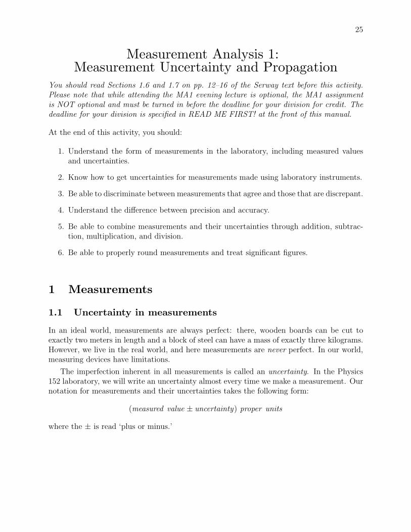
9.800 9.802 9.804 9.8069.7989.7969.794
9.801 m/s2
m/s2
26 Purdue University Physics 152L Measurement Analysis 1
Figure 1: Measurement and uncertainty: (9.801± 0.003) m/s2
Consider the measurement g = (9.801 ± 0.003) m/s2. We interpret this measurementas meaning that the experimentally determined value of g can lie anywhere between thevalues 9.801 + 0.003 m/s2 and 9.801 − 0.003 m/s2, or 9.798 m/s2 ≤ g ≤ 9.804 m/s2. Asyou can see, a real world measurement is not one simple measured value, but is actually arange of possible values (see Figure 1). This range is determined by the uncertainty in themeasurement. As uncertainty is reduced, this range is narrowed.
Here are two examples of measurements:
v = (4.000± 0.002) m/s G = (6.67± 0.01)× 10−11 N·m2/kg2
Look over the measurements given above, paying close attention to the number of decimalplaces in the measured values and the uncertainties (when the measurement is good to thethousandths place, so is the uncertainty; when the measurement is good to the hundredthsplace, so is the uncertainty). You should notice that they always agree, and this is mostimportant:
— In a measurement, the measured value and its uncertainty must always havethe same number of digits after the decimal place.
Examples of nonsensical measurements are (9.8 ± 0.0001) m/s2 and (9.801 ± 0.1) m/s2;writing such nonsensical measurements will cause readers to judge you as either incompetentor sloppy. Avoid writing improper measurements by always making sure the decimal placesagree.
Sometimes we want to talk about measurements more generally, and so we write themwithout actual numbers. In these cases, we use the lowercase Greek letter delta, or δ torepresent the uncertainty in the measurement. Examples include:
(X ± δX) (Y ± δY )
Although units are not explicitly written next to these measurements, they are implied.We will use these general expressions for measurements when we discuss the propagation ofuncertainties in Section 4.
1.2 Uncertainties in measurements in lab
In the laboratory you will be taking real world measurements, and for some measurementsyou will record both measured values and uncertainties. Getting values from measuring
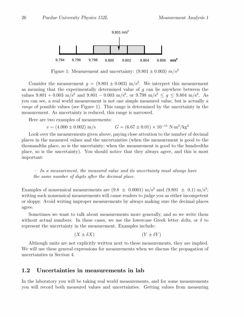
0 2 4 6 8 10 12 cm
(L ± δL) = (6 ± 1) cm
Purdue University Physics 152L Measurement Analysis 1 27
equipment is usually as simple as reading a scale or a digital readout. Determining uncer-tainties is a bit more challenging since you—not the measuring device— must determinethem. When determining an uncertainty from a measuring device, you need to first deter-mine the smallest quantity that can be resolved on the device. Then, for your work in PHYS152L, the uncertainty in the measurement is taken to be this value. For example, if a digitalreadout displays 1.35 g, then you should write that measurement as (1.35 ± 0.01) g. Thesmallest division you can clearly read is your uncertainty.
On the other hand, reading a scale is somewhat subjective. Suppose you use a meter stickthat is divided into centimeters to determine the length (L ± δL) of a rod, as illustrated inFigure 2. First, you read your measured value from this scale and find that the rod is 6 cm.Depending on the sharpness of your vision, the clarity of the scale, and the boundaries ofthe measured object, you might read the uncertainty as ± 1 cm, ± 0.5 cm, or ± 0.2 cm. Anuncertainty of ± 0.1 cm or smaller is dubious because the ends of the object are roundedand it is hard to resolve ± 0.1 cm. Thus, you might want to record your measurement as(L ± δL) = (6 ± 1) cm, (L ± δL) = (6.0 ± 0.5) cm, or (L ± δL) = (6.0 ± 0.2) cm,since all three measurements would appear reasonable. For the purposes of discussion anduniformity in this laboratory manual, we will use the largest reasonable uncertainty. For ourexample, this is ± 1 cm.
Figure 2: A measurement obtained by reading a scale. Acceptable measurements range from6.0 ± 0.1 cm to 6.0 ± 0.2 cm, depending on the sharpness of your vision, the clarity of thescale, and the boundaries of the measured object. Examples of unacceptable measurementsare 6± 2 cm and 6.00± 0.01 cm.
1.3 Percentage uncertainty of measurements
When we speak of a measurement, we often want to know how reliable it is. We needsome way of judging the relative worth of a measurement, and this is done by finding thepercentage uncertainty of a measurement. We will refer to the percentage uncertainty of ameasurement as the ratio between the measurement’s uncertainty and its measured valuemultiplied by 100%. You will often hear this kind of uncertainty or something closely relatedused with measurements – a meter is good to ± 3% of full scale, or ± 1% of the reading, orgood to one part in a million.
The percentage uncertainty of a measurement (Z ± δZ) is defined asδZ
Z× 100%.
Think about percentage uncertainty as a way of telling how much a measurement de-viates from “perfection.” With this idea in mind, it makes sense that as the uncertainty
28 Purdue University Physics 152L Measurement Analysis 1
for a measurement decreases, the percentage uncertainty δZZ× 100% decreases, and so the
measurement deviates less from perfection. For example, a measurement of (2 ± 1) mhas a percentage uncertainty of 50%, or one part in two. In contrast, a measurement of(2.00 ± 0.01) m has a percentage uncertainty of 0.5% (or 1 part in 200) and is thereforethe more precise measurement. If there were some way to make this same measurementwith zero uncertainty, the percentage uncertainty would equal 0% and there would be nodeviation whatsoever from the measured value—we would have a “perfect” measurement.Unfortunately, this never happens in the real world.
1.4 Implied uncertainties
When you read a physics textbook, you may notice that almost all the measurements statedare missing uncertainties. Does this mean that the author is able to measure things perfectly,without any uncertainty? Not at all! In fact, it is common practice in textbooks not to writeuncertainties with measurements, even though they are actually there. In such cases, theuncertainties are implied. We treat these implied uncertainties the same way as we did whentaking measurements in lab:
— In a measurement with an implied uncertainty, the actual uncertainty is writ-ten as ± 1 in the smallest place value of the given measured value.
For example, if you read g = 9.80146 m/s2 in a textbook, you know this measured valuehas an implied uncertainty of 0.00001 m/s2. To be more specific, you could then write(g ± δg) = (9.80146 ± 0.00001) m/s2.
1.5 Decimal points — don’t lose them
If a decimal point gets lost, it can have disastrous consequences. One of the most commonplaces where a decimal point gets lost is in front of a number. For example, writing .52 cmsometimes results in a reader missing the decimal point, and reading it as 52 cm — onehundred times larger! After all, a decimal point is only a simple small dot. However, writing0.52 cm virtually eliminates the problem, and writing leading zeros for decimal numbers isstandard scientific and engineering practice.
2 Agreement, Discrepancy, and Difference
In the laboratory, you will not only be taking measurements, but also comparing them.You will compare your experimental measurements (i.e. the ones you find in lab) to sometheoretical, predicted, or standard measurements (i.e. the type you calculate or look up ina textbook) as well as to experimental measurements you make during a second (or third...)data run. We need a method to determine how closely these measurements compare.
To simplify this process, we adopt the following notion: two measurements, when com-pared, either agree within experimental uncertainty or they are discrepant (that is, they do
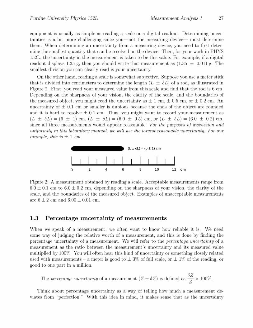
9.790 9.800 9.810m/(s*s)
g exp
g std
a: two values in experimental agreement
9.790 9.800 9.810m/(s*s)
g exp
g std
b: two discrepant values
Purdue University Physics 152L Measurement Analysis 1 29
not agree). Before we illustrate how this classification is carried out, you should first recallthat a measurement in the laboratory is not made up of one single value, but a whole rangeof values. With this in mind, we can say,
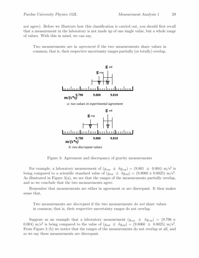
Two measurements are in agreement if the two measurements share values incommon; that is, their respective uncertainty ranges partially (or totally) overlap.
Figure 3: Agreement and discrepancy of gravity measurements
For example, a laboratory measurement of (gexp ± δgexp) = (9.801 ± 0.004) m/s2 isbeing compared to a scientific standard value of (gstd ± δgstd) = (9.8060 ± 0.0025) m/s2.As illustrated in Figure 3(a), we see that the ranges of the measurements partially overlap,and so we conclude that the two measurements agree.
Remember that measurements are either in agreement or are discrepant. It then makessense that,
Two measurements are discrepant if the two measurements do not share valuesin common; that is, their respective uncertainty ranges do not overlap.
Suppose as an example that a laboratory measurement (gexp ± δgexp) = (9.796 ±0.004) m/s2 is being compared to the value of (gstd ± δgstd) = (9.8060 ± 0.0025) m/s2.From Figure 3 (b) we notice that the ranges of the measurements do not overlap at all, andso we say these measurements are discrepant.
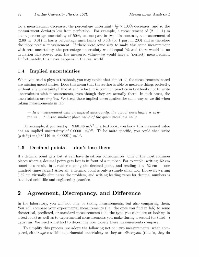
Precision & Accuracy
precise, but not accurate
accurate, but notprecise
(a) (b)
30 Purdue University Physics 152L Measurement Analysis 1
When two measurements being compared do not agree, we want to know by how muchthey do not agree. We call this quantity the discrepancy between measurements, and we usethe following formula to compute it:
The discrepancy Z between an experimental measurement (X ± δX) and a theoreticalor standard measurement (Y ± δY ) is:
Z =Xexperimental − Ystandard
Ystandard× 100%
As an example, take the two discrepant measurements (gexp ± δgexp) and (gstd ± δgstd) fromthe previous example. Since we found that these two measurements are discrepant, we cancalculate the discrepancy Z between them as:
Z =gexp − gstd
gstd× 100% =
9.796− 9.8060
9.8060× 100% ≈ −0.10%
Keep the following in mind when comparing measurements in the laboratory:
1. If you find that two measurements agree, state this in your report. Do NOT computea discrepancy.
2. If you find that two measurements are discrepant, state this in your report and thengo on to compute the discrepancy.
3 Precision and accuracy
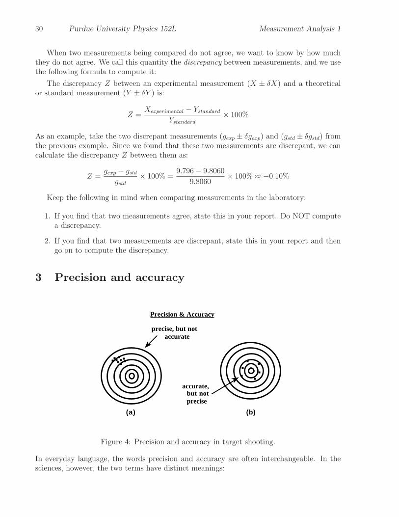
Figure 4: Precision and accuracy in target shooting.
In everyday language, the words precision and accuracy are often interchangeable. In thesciences, however, the two terms have distinct meanings:
1 2 3a: neither accurate nor precise
1 2 3b: precise, but not accurate
1 2 3c: both accurate and precise
Purdue University Physics 152L Measurement Analysis 1 31
Precision describes the degree of certainty one has about a measurement.
Accuracy describes how well measurements agree with a known, standard mea-surement.
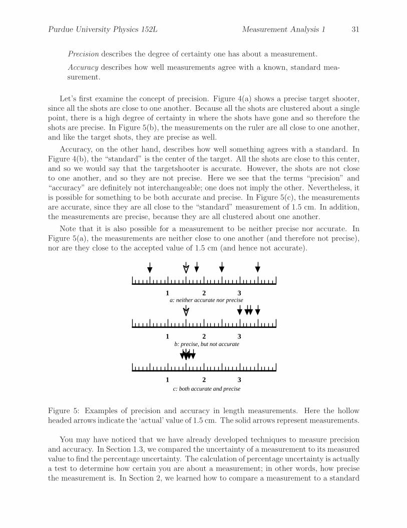
Let’s first examine the concept of precision. Figure 4(a) shows a precise target shooter,since all the shots are close to one another. Because all the shots are clustered about a singlepoint, there is a high degree of certainty in where the shots have gone and so therefore theshots are precise. In Figure 5(b), the measurements on the ruler are all close to one another,and like the target shots, they are precise as well.
Accuracy, on the other hand, describes how well something agrees with a standard. InFigure 4(b), the “standard” is the center of the target. All the shots are close to this center,and so we would say that the targetshooter is accurate. However, the shots are not closeto one another, and so they are not precise. Here we see that the terms “precision” and“accuracy” are definitely not interchangeable; one does not imply the other. Nevertheless, itis possible for something to be both accurate and precise. In Figure 5(c), the measurementsare accurate, since they are all close to the “standard” measurement of 1.5 cm. In addition,the measurements are precise, because they are all clustered about one another.
Note that it is also possible for a measurement to be neither precise nor accurate. InFigure 5(a), the measurements are neither close to one another (and therefore not precise),nor are they close to the accepted value of 1.5 cm (and hence not accurate).
Figure 5: Examples of precision and accuracy in length measurements. Here the hollowheaded arrows indicate the ‘actual’ value of 1.5 cm. The solid arrows represent measurements.
You may have noticed that we have already developed techniques to measure precisionand accuracy. In Section 1.3, we compared the uncertainty of a measurement to its measuredvalue to find the percentage uncertainty. The calculation of percentage uncertainty is actuallya test to determine how certain you are about a measurement; in other words, how precisethe measurement is. In Section 2, we learned how to compare a measurement to a standard
32 Purdue University Physics 152L Measurement Analysis 1
or accepted value by calculating a percent discrepancy. This comparison told you how closeyour measurement was to this standard measurement, and so finding percent discrepancy isreally a test for accuracy.
It turns out that in the laboratory, precision is much easier to achieve than accuracy.Precision can be achieved by careful techniques and handiwork, but accuracy requires ex-cellence in experimental design and measurement analysis. During this laboratory course,you will examine both accuracy and precision in your measurements and suggest methodsof improving both.
4 Propagation of uncertainty (worst case)
In the laboratory, we will need to combine measurements using addition, subtraction, mul-tiplication, and division. However, measurements are composed of two parts—a measuredvalue and an uncertainty—and so any algebraic combination must account for both. Perform-ing these operations on the measured values is easily accomplished; handling uncertaintiesposes the challenge. We make use of the propagation of uncertainty to combine measurementswith the assumption that as measurements are combined, uncertainty increases—hence theuncertainty propagates through the calculation. Here we show how to combine two mea-surements and their uncertainties. Often in lab you will have to keep using the propagationformulae over and over, building up more and more uncertainty as you combine three, fouror five set of numbers.
1. When adding two measurements, the uncertainty in the final measurement is thesum of the uncertainties in the original measurements:
(A± δA) + (B ± δB) = (A+B)± (δA+ δB) (1)
As an example, let us calculate the combined length (L ± δL) of two tables whoselengths are (L1 ± δL1) = (3.04 ± 0.04) m and (L2 ± δL2) = (10.30 ± 0.01) m. Usingthis addition rule, we find that
(L± δL) = (3.04± 0.04) m + (10.30± 0.01) m = (13.34± 0.05) m
2. When subtracting two measurements, the uncertainty in the final measurementis again equal to the sum of the uncertainties in the original measurements:
(A± δA)− (B ± δB) = (A−B)± (δA+ δB) (2)
For example, the difference in length between the two tables mentioned above is
(L2 ± δL2)− (L1 ± δL1) = (10.30± 0.01) m− (3.04± 0.04) m
= [(10.30− 3.04)± (0.01 + 0.04)] m
= (7.26± 0.05) m
Purdue University Physics 152L Measurement Analysis 1 33
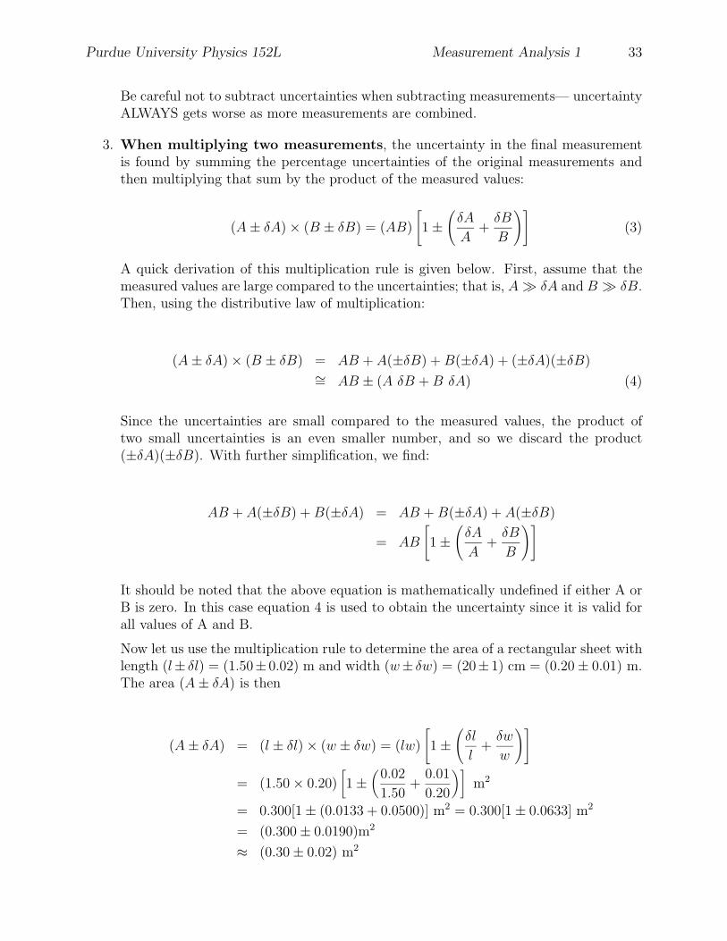
Be careful not to subtract uncertainties when subtracting measurements— uncertaintyALWAYS gets worse as more measurements are combined.
3. When multiplying two measurements, the uncertainty in the final measurementis found by summing the percentage uncertainties of the original measurements andthen multiplying that sum by the product of the measured values:
(A± δA)× (B ± δB) = (AB)
[1±
(δA
A+δB
B
)](3)
A quick derivation of this multiplication rule is given below. First, assume that themeasured values are large compared to the uncertainties; that is, AÀ δA and B À δB.Then, using the distributive law of multiplication:
(A± δA)× (B ± δB) = AB + A(±δB) +B(±δA) + (±δA)(±δB)∼= AB ± (A δB +B δA) (4)
Since the uncertainties are small compared to the measured values, the product oftwo small uncertainties is an even smaller number, and so we discard the product(±δA)(±δB). With further simplification, we find:
AB + A(±δB) +B(±δA) = AB +B(±δA) + A(±δB)
= AB
[1±
(δA
A+δB
B
)]
It should be noted that the above equation is mathematically undefined if either A orB is zero. In this case equation 4 is used to obtain the uncertainty since it is valid forall values of A and B.
Now let us use the multiplication rule to determine the area of a rectangular sheet withlength (l± δl) = (1.50± 0.02) m and width (w± δw) = (20± 1) cm = (0.20± 0.01) m.The area (A± δA) is then
(A± δA) = (l ± δl)× (w ± δw) = (lw)
[1±
(δl
l+δw
w
)]
= (1.50× 0.20)[1±
(0.02
1.50+
0.01
0.20
)]m2
= 0.300[1± (0.0133 + 0.0500)] m2 = 0.300[1± 0.0633] m2
= (0.300± 0.0190)m2
≈ (0.30± 0.02) m2
34 Purdue University Physics 152L Measurement Analysis 1
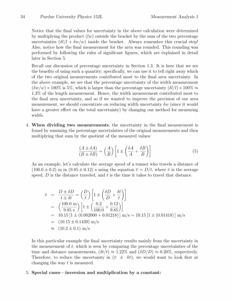
Notice that the final values for uncertainty in the above calculation were determinedby multiplying the product (lw) outside the bracket by the sum of the two percentageuncertainties (δl/l + δw/w) inside the bracket. Always remember this crucial step!Also, notice how the final measurement for the area was rounded. This rounding wasperformed by following the rules of significant figures, which are explained in detaillater in Section 5.
Recall our discussion of percentage uncertainty in Section 1.3. It is here that we seethe benefits of using such a quantity; specifically, we can use it to tell right away whichof the two original measurements contributed most to the final area uncertainty. Inthe above example, we see that the percentage uncertainty of the width measurement(δw/w)×100% is 5%, which is larger than the percentage uncertainty (δl/l)×100% ≈1.3% of the length measurement. Hence, the width measurement contributed most tothe final area uncertainty, and so if we wanted to improve the precision of our areameasurement, we should concentrate on reducing width uncertainty δw (since it wouldhave a greater effect on the total uncertainty) by changing our method for measuringwidth.
4. When dividing two measurements, the uncertainty in the final measurement isfound by summing the percentage uncertainties of the original measurements and thenmultiplying that sum by the quotient of the measured values:
(A± δA)
(B ± δB)=(A
B
) [1±
(δA
A+δB
B
)](5)
As an example, let’s calculate the average speed of a runner who travels a distance of(100.0± 0.2) m in (9.85± 0.12) s using the equation v = D/t, where v̄ is the averagespeed, D is the distance traveled, and t is the time it takes to travel that distance.
v̄ =D ± δDt± δt =
(D
t
) [1±
(δD
D+δt
t
)]
=(
100.0 m
9.85 s
) [1±
(0.2
100.0+
0.12
9.85
)]= 10.15 [1± (0.002000 + 0.01218) ] m/s = 10.15 [1± (0.01418) ] m/s
= (10.15± 0.1439) m/s
≈ (10.2± 0.1) m/s
In this particular example the final uncertainty results mainly from the uncertainty inthe measurement of t, which is seen by comparing the percentage uncertainties of thetime and distance measurements, (δt/t) ≈ 1.22% and (δD/D) ≈ 0.20%, respectively.Therefore, to reduce the uncertainty in (v ± δv), we would want to look first atchanging the way t is measured.
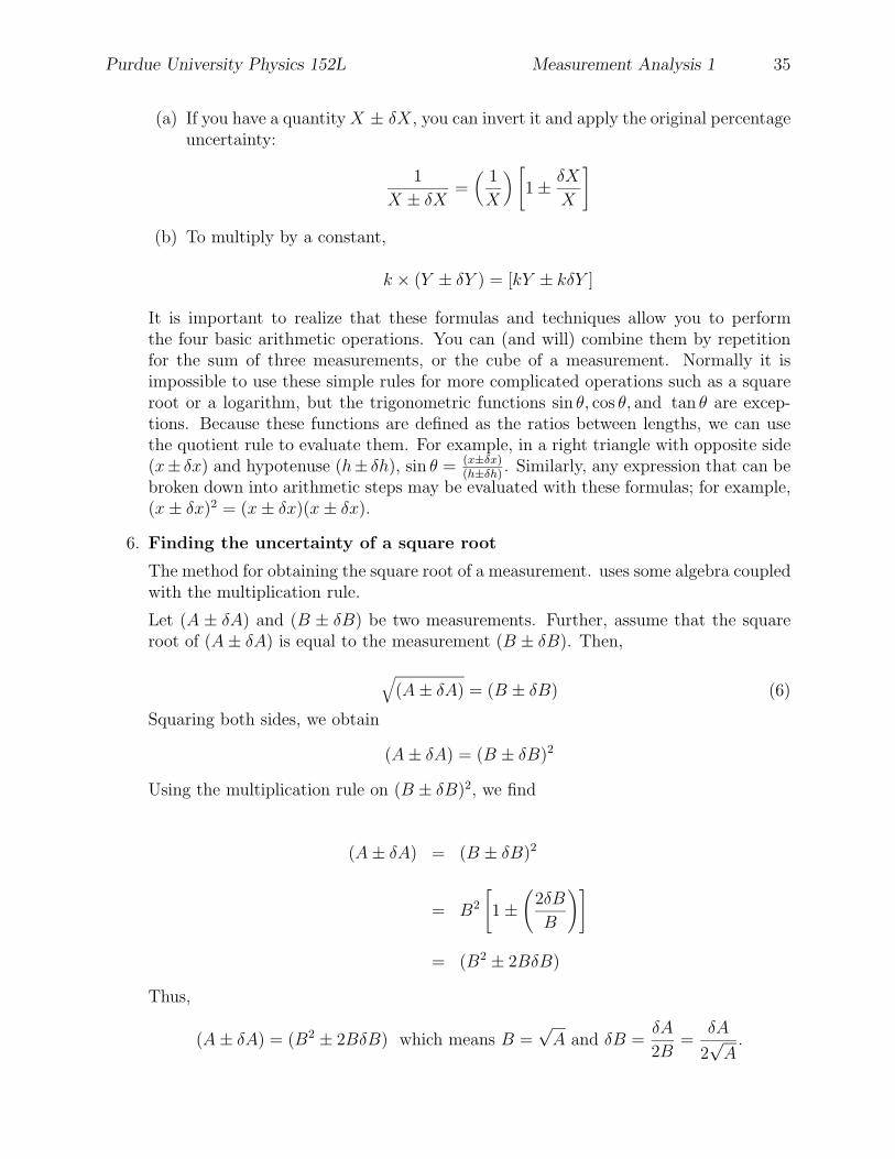
5. Special cases—inversion and multiplication by a constant:
Purdue University Physics 152L Measurement Analysis 1 35
(a) If you have a quantity X ± δX, you can invert it and apply the original percentageuncertainty:
1
X ± δX =(
1
X
) [1± δX
X
]
(b) To multiply by a constant,
k × (Y ± δY ) = [kY ± kδY ]
It is important to realize that these formulas and techniques allow you to performthe four basic arithmetic operations. You can (and will) combine them by repetitionfor the sum of three measurements, or the cube of a measurement. Normally it isimpossible to use these simple rules for more complicated operations such as a squareroot or a logarithm, but the trigonometric functions sin θ, cos θ, and tan θ are excep-tions. Because these functions are defined as the ratios between lengths, we can usethe quotient rule to evaluate them. For example, in a right triangle with opposite side(x± δx) and hypotenuse (h± δh), sin θ = (x±δx)
(h±δh). Similarly, any expression that can be
broken down into arithmetic steps may be evaluated with these formulas; for example,(x± δx)2 = (x± δx)(x± δx).
6. Finding the uncertainty of a square root
The method for obtaining the square root of a measurement. uses some algebra coupledwith the multiplication rule.
Let (A ± δA) and (B ± δB) be two measurements. Further, assume that the squareroot of (A± δA) is equal to the measurement (B ± δB). Then,
√(A± δA) = (B ± δB) (6)
Squaring both sides, we obtain
(A± δA) = (B ± δB)2
Using the multiplication rule on (B ± δB)2, we find
(A± δA) = (B ± δB)2
= B2
[1±
(2δB
B
)]
= (B2 ± 2BδB)
Thus,
(A± δA) = (B2 ± 2BδB) which means B =√A and δB =
δA
2B=
δA
2√A.
36 Purdue University Physics 152L Measurement Analysis 1
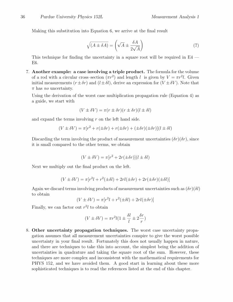
Making this substitution into Equation 6, we arrive at the final result
√(A± δA) =
(√A± δA
2√A
)(7)
This technique for finding the uncertainty in a square root will be required in E4 —E6.
7. Another example: a case involving a triple product. The formula for the volumeof a rod with a circular cross–section (πr2) and length l is given by V = πr2l. Giveninitial measurements (r± δr) and (l± δl), derive an expression for (V ± δV ). Note thatπ has no uncertainty.
Using the derivation of the worst case multiplication propagation rule (Equation 4) asa guide, we start with
(V ± δV ) = π(r ± δr)(r ± δr)(l ± δl)
and expand the terms involving r on the left hand side.
(V ± δV ) = π[r2 + r(±δr) + r(±δr) + (±δr)(±δr)](l ± δl)
Discarding the term involving the product of measurement uncertainties (δr)(δr), sinceit is small compared to the other terms, we obtain
(V ± δV ) = π[r2 + 2r(±δr)](l ± δl)
Next we multiply out the final product on the left.
(V ± δV ) = π[r2l + r2(±δl) + 2rl(±δr) + 2r(±δr)(±δl)]
Again we discard terms involving products of measurement uncertainties such as (δr)(δl)to obtain
(V ± δV ) = π[r2l + r2(±δl) + 2rl(±δr)]Finally, we can factor out r2l to obtain
(V ± δV ) = πr2l(1± δl
l± 2
δr
r)
8. Other uncertainty propagation techniques. The worst case uncertainty propa-gation assumes that all measurement uncertainties conspire to give the worst possibleuncertainty in your final result. Fortunately this does not usually happen in nature,and there are techniques to take this into account, the simplest being the addition ofuncertainties in quadrature and taking the square root of the sum. However, thesetechniques are more complex and inconsistent with the mathematical requirements forPHYS 152, and we have avoided them. A good start in learning about these moresophisticated techniques is to read the references listed at the end of this chapter.
Purdue University Physics 152L Measurement Analysis 1 37
5 Rounding measurements
The previous sections contain the bulk of what you need to take and analyze measurementsin the laboratory. Now it is time to discuss the finer details of measurement analysis. Thesubtleties we are about to present cause an inordinate amount of confusion in the laboratory.Getting caught up in details is a frustrating experience, and the following guidelines shouldhelp alleviate these problems.
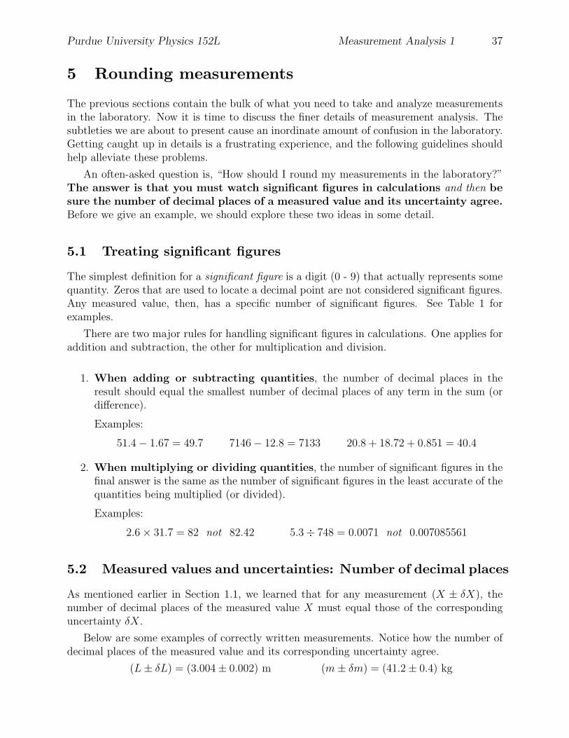
An often-asked question is, “How should I round my measurements in the laboratory?”The answer is that you must watch significant figures in calculations and then besure the number of decimal places of a measured value and its uncertainty agree.Before we give an example, we should explore these two ideas in some detail.
5.1 Treating significant figures
The simplest definition for a significant figure is a digit (0 - 9) that actually represents somequantity. Zeros that are used to locate a decimal point are not considered significant figures.Any measured value, then, has a specific number of significant figures. See Table 1 forexamples.
There are two major rules for handling significant figures in calculations. One applies foraddition and subtraction, the other for multiplication and division.
1. When adding or subtracting quantities, the number of decimal places in theresult should equal the smallest number of decimal places of any term in the sum (ordifference).
Examples:
51.4− 1.67 = 49.7 7146− 12.8 = 7133 20.8 + 18.72 + 0.851 = 40.4
2. When multiplying or dividing quantities, the number of significant figures in thefinal answer is the same as the number of significant figures in the least accurate of thequantities being multiplied (or divided).
Examples:
2.6× 31.7 = 82 not 82.42 5.3÷ 748 = 0.0071 not 0.007085561
5.2 Measured values and uncertainties: Number of decimal places
As mentioned earlier in Section 1.1, we learned that for any measurement (X ± δX), thenumber of decimal places of the measured value X must equal those of the correspondinguncertainty δX.
Below are some examples of correctly written measurements. Notice how the number ofdecimal places of the measured value and its corresponding uncertainty agree.
(L± δL) = (3.004± 0.002) m (m± δm) = (41.2± 0.4) kg
38 Purdue University Physics 152L Measurement Analysis 1
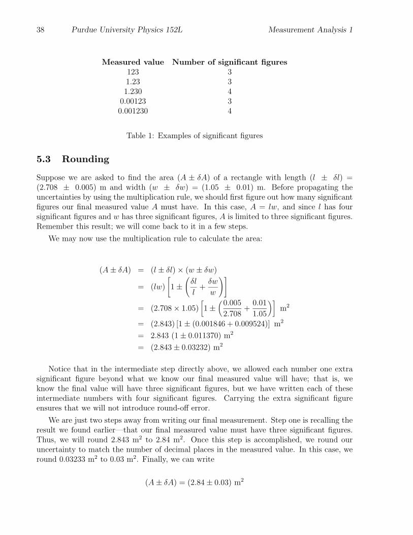
Measured value Number of significant figures123 31.23 31.230 4
0.00123 30.001230 4
Table 1: Examples of significant figures
5.3 Rounding
Suppose we are asked to find the area (A ± δA) of a rectangle with length (l ± δl) =(2.708 ± 0.005) m and width (w ± δw) = (1.05 ± 0.01) m. Before propagating theuncertainties by using the multiplication rule, we should first figure out how many significantfigures our final measured value A must have. In this case, A = lw, and since l has foursignificant figures and w has three significant figures, A is limited to three significant figures.Remember this result; we will come back to it in a few steps.
We may now use the multiplication rule to calculate the area:
(A± δA) = (l ± δl)× (w ± δw)
= (lw)
[1±
(δl
l+δw
w
)]
= (2.708× 1.05)[1±
(0.005
2.708+
0.01
1.05
)]m2
= (2.843) [1± (0.001846 + 0.009524)] m2
= 2.843 (1± 0.011370) m2
= (2.843± 0.03232) m2
Notice that in the intermediate step directly above, we allowed each number one extrasignificant figure beyond what we know our final measured value will have; that is, weknow the final value will have three significant figures, but we have written each of theseintermediate numbers with four significant figures. Carrying the extra significant figureensures that we will not introduce round-off error.
We are just two steps away from writing our final measurement. Step one is recalling theresult we found earlier—that our final measured value must have three significant figures.Thus, we will round 2.843 m2 to 2.84 m2. Once this step is accomplished, we round ouruncertainty to match the number of decimal places in the measured value. In this case, weround 0.03233 m2 to 0.03 m2. Finally, we can write
(A± δA) = (2.84± 0.03) m2
Purdue University Physics 152L Measurement Analysis 1 39
6 References
These books are on reserve in the Physics Library (PHYS 291). Ask for them by the author’slast name.
1. Bevington, P. R., Data reduction and uncertainty analysis for the physical sciences(McGraw-Hill, New York, 1969).
2. Young, H. D., Statistical treatment of experimental data (McGraw-Hill, New York,1962).

40 Purdue University Physics 152L Measurement Analysis 1
This page is deliberately left blank.
1 2 3 cm0
A B C D
Purdue University Physics 152L Measurement Analysis 1 41
Measurement Analysis Problem Set MA1Name Lab day/time
Division GTA
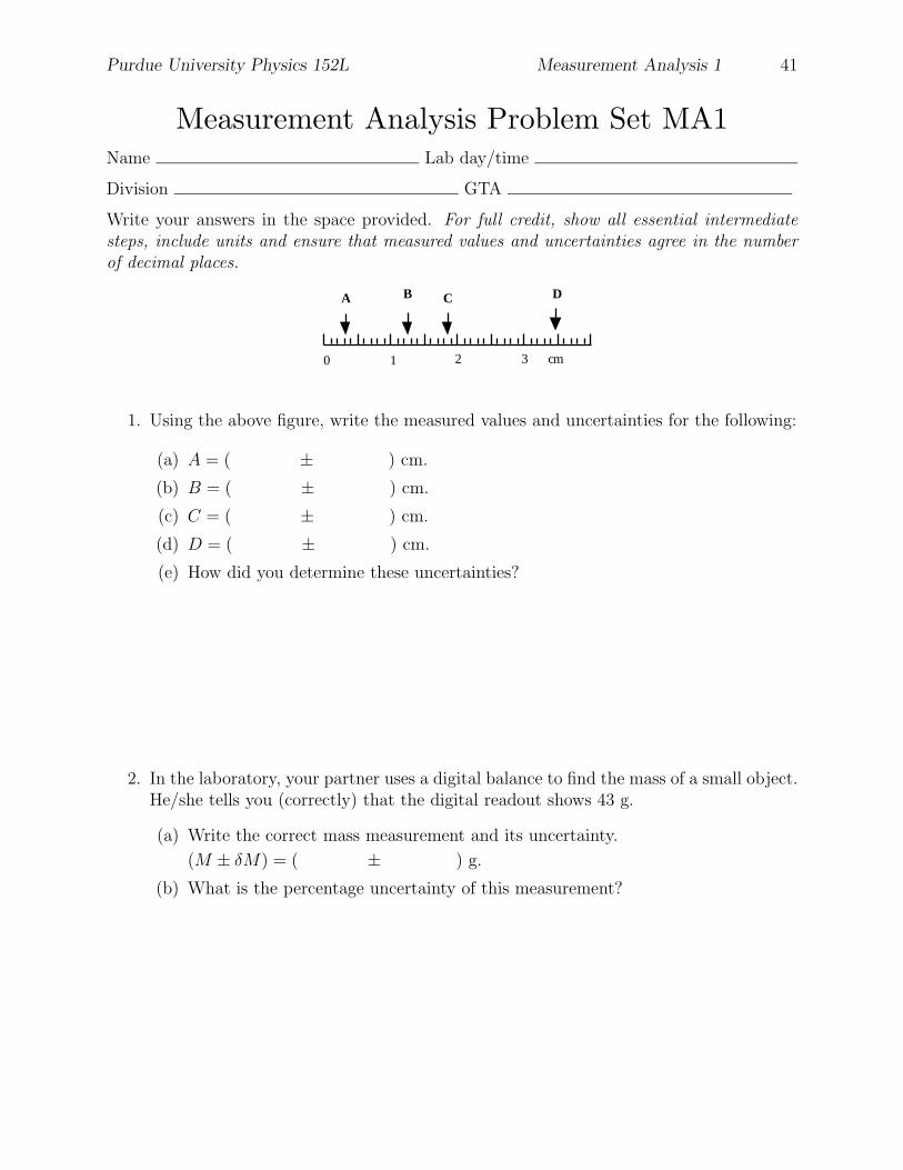
Write your answers in the space provided. For full credit, show all essential intermediatesteps, include units and ensure that measured values and uncertainties agree in the numberof decimal places.
1. Using the above figure, write the measured values and uncertainties for the following:
(a) A = ( ± ) cm.
(b) B = ( ± ) cm.
(c) C = ( ± ) cm.
(d) D = ( ± ) cm.
(e) How did you determine these uncertainties?
2. In the laboratory, your partner uses a digital balance to find the mass of a small object.He/she tells you (correctly) that the digital readout shows 43 g.
(a) Write the correct mass measurement and its uncertainty.
(M ± δM) = ( ± ) g.
(b) What is the percentage uncertainty of this measurement?
42 Purdue University Physics 152L Measurement Analysis 1
3. In lab, one of your partners determines (correctly) that the surface area of an objectis 25.97 cm2. All of the figures in this measurement are significant.
(a) Your HP-9000 calculator tells you that the uncertainty is 0.04382361 cm2. Writethe appropriate measurement and its uncertainty.
(A± δA) = ( ± ) cm2
(b) Alternatively, your HP-9000 told you that the uncertainty is 0.0012543797 cm2.Write the appropriate measurement and its uncertainty.
(A± δA) = ( ± ) cm2
(c) Finally, the calculator told you that the uncertainty is 0.017386642 cm2. Writethe appropriate measurement and its uncertainty.
(A± δA) = ( ± ) cm2
(d) Briefly explain how you determined these three numerical uncertainties.
4. In the laboratory you determine the gravitational constant (gexp ± δgexp) to be(9.824± 0.006) m/s2. According to a geophysical survey, the accepted local value for(gacc ± δgacc) is (9.802± 0.002) m/s2.
(a) Draw a diagram like Figure 3 showing whether your measurement agrees with theaccepted value within the limits of experimental uncertainty or not.
(b) If these measures do not agree, what is the actual discrepancy?
Purdue University Physics 152L Measurement Analysis 1 43
5. For a laboratory exercise, you determine the masses of two airtrack gliders as(m1 ± δm1) = (484.9 ± 0.3) g and (m2 ± δm2) = (314.2 ± 0.1) g. Determinethe following combinations of the measurements, and show your work.
(a) (m2 ± δm2)− (m1 ± δm1) = ( ± ) g.
(b) Determine the precisions of the measurements (m1 ± δm1) and (m2 ± δm2).Which calculated precision is the larger? Using this information, determine whichis the better measurement.
(c) (m1 ± δm1) + (m2 ± δm2) = ( ± ) g.
6. (a) Laboratory measurements performed upon a rectangular steel plate show thelength (l ± δl) = (2.41 ± 0.25) cm and the width (w ± δw) = (8.30 ± 0.10) cm.Determine the area of the steel plate and the uncertainty in the area.
A± δA = ( ± ) cm2.
(b) As Director of the National Science Foundation, you must decide what is thebest means to improve the precision of the area measurement of the steel plate.You can spend money on a space gizmotron to better measure length, or on asuperconducting whizbang to better measure width, but not both. On whichmeasurement should you spend the money? Justify your decision with numbers.
44 Purdue University Physics 152L Measurement Analysis 1
7. During another airtrack experiment, you determine the initial position of a glider tobe (xi ± δxi) = (0.482 ± 0.001) m and its final position to be (xf ± δxf ) =(0.633 ± 0.003) m, with an elapsed time (t ± δt) = (0.48 ± 0.01) s during thedisplacement.
(a) Find the total displacement of the glider (D ± δD) = (xf ± δxf )− (xi ± δxi).(D ± δD) = ( ± ) m.
(b) Find the average speed of the glider (v̄glider ± δv̄glider) = (D ± δD)/(t ± δt).v̄glider ± δv̄glider = ( ± ) m/s.
(c) Calculate the percentage uncertainties for the two quantities (D±δD) and (t±δt).Based on these precisions, determine which of the two quantities contributes mostto the overall uncertainty δv̄glider.
(d) If we could change the apparatus so as to measure either distance or time tentimes more accurately (but not both), which should we change and why?
Purdue University Physics 152L Measurement Analysis 1 45
8. In the laboratory, a measurement for (x± δx) was taken as (x± δx) = (33.4± 0.5) s2.Write a value for its reciprocal. Show calculations, and ensure that you handle signifi-cant figures properly.
1(x±δx)
= ( ± ) 1s2 .
9. The formula for the volume of a box with height h , base b , and length l is given byV = bhl. Given initial measurements (h ± δh), (b ± δb), and (l ± δl), derive anexpression for (V ± δV ). Do NOT use the multiplication rule (Equation 3) in derivingthis equation.
Hint: Use the derivation of the worst case multiplication propagation rule (Equation 4)as a guide. Start with (V ± δV ) = (b± δb)(h± δh)(l± δl). Expand, show intermediatesteps, and regroup and simplify your solution as much as possible. Discard productsof measurement uncertainties, such as (δh)(δb)(l) and (δh)(δb)(δl).