measurement and analysis of household carbon: the...
TRANSCRIPT

This work is licensed under a Creative Commons Attribution 4.0 International License
Newcastle University ePrints - eprint.ncl.ac.uk
Allinson A, Irvine KN, Edmondson JL, Tiwary A, Hill G, Morris J, Bell M, Davies
ZG, Firth SK, Fisher J, Gaston KJ, Leake JR, McHugh N, Namdeo A, Rylatt M,
Lomas K. Measurement and analysis of household carbon: the case of a UK
city. Applied Energy 2016, 164, 871–881.
Copyright:
© 2015 The Authors. Published by Elsevier Ltd. This is an open access article under the CC BY license
(http://creativecommons.org/licenses/by/4.0/).
DOI link to article:
http://dx.doi.org/10.1016/j.apenergy.2015.11.054
Date deposited:
12/01/2016
Applied Energy 164 (2016) 871–881
Contents lists available at ScienceDirect
Applied Energy
journal homepage: www.elsevier .com/locate /apenergy
Measurement and analysis of household carbon: The case of a UK city
http://dx.doi.org/10.1016/j.apenergy.2015.11.0540306-2619/� 2015 The Authors. Published by Elsevier Ltd.This is an open access article under the CC BY license (http://creativecommons.org/licenses/by/4.0/).
⇑ Corresponding author. Tel.: +44 (0)1509 223643.E-mail address: [email protected] (D. Allinson).
David Allinson a,⇑, Katherine N. Irvine b,c, Jill L. Edmondson d, Abhishek Tiwary e, Graeme Hill f,Jonathan Morris g, Margaret Bell f, Zoe G. Davies h, Steven K. Firth a, Jill Fisher c, Kevin J. Gaston i,Jonathan R. Leake d, Nicola McHugh d, Anil Namdeo f, Mark Rylatt c, Kevin Lomas a
a School of Civil and Building Engineering, Loughborough University, Leicestershire LE11 3TU, UKb Social, Economic and Geographical Sciences, James Hutton Institute, Craigiebuckler, Aberdeen AB15 8QH, UKc Institute of Energy and Sustainable Development, Queens Building, De Montfort University, The Gateway, Leicester LE1 9BH, UKdDepartment of Animal & Plant Sciences, The University of Sheffield, Alfred Denny Building, Western Bank, Sheffield S10 2TN, UKe Faculty of Engineering and the Environment, University of Southampton, Highfield, Southampton SO17 1BJ, UKf School of Civil Engineering and Geosciences, Cassie Building, Newcastle University, Newcastle upon Tyne NE1 7RU, UKgCentre for Energy, Environment and Sustainability, The University of Sheffield, ICOSS Building, 219 Portobello, Sheffield S1 4DP, UKhDurrell Institute of Conservation and Ecology, University of Kent, Canterbury, Kent CT2 7NR, UKiEnvironment and Sustainability Institute, University of Exeter, Penryn, Cornwall TR10 9EZ, UK
h i g h l i g h t s
� Median annual carbon emissions from household end-use energy demand was 6744 kg CO2e.� One third of the households were responsible for over half of the carbon emissions.� There was considerable organic carbon stored in gardens.� Emissions from transport, gas and electricity demands should all be considered.� An individual emissions source cannot be used as a marker for high total emissions.
a r t i c l e i n f o
Article history:Received 30 July 2015Received in revised form 18 October 2015Accepted 29 November 2015
Keywords:Domestic energy demandHousehold emissionsTransport emissionsOrganic carbon storageEnergy policy
a b s t r a c t
There is currently a lack of data recording the carbon and emissions inventory at household level. Thispaper presents a multi-disciplinary, bottom-up approach for estimation and analysis of the carbonemissions, and the organic carbon (OC) stored in gardens, using a sample of 575 households across aUK city. The annual emission of carbon dioxide emissions from energy used in the homes was measured,personal transport emissions were assessed through a household survey and OC stores estimated fromsoil sampling and vegetation surveys. The results showed that overall carbon patterns were skewed withhighest emitting third of the households being responsible for more than 50% of the emissions andaround 50% of garden OC storage. There was diversity in the relative contribution that gas, electricityand personal transport made to each household’s total and different patterns were observed for high,medium and low emitting households. Targeting households with high carbon emissions from one sourcewould not reliably identify them as high emitters overall. While carbon emissions could not be offset bygrowing trees in gardens, there were considerable amounts of stored OC in gardens which ought to beprotected. Exploratory analysis of the multiple drivers of emissions was conducted using a combinationof primary and secondary data. These findings will be relevant in devising effective policy instruments forcombatting city scale green-house gas emissions from domestic end-use energy demand.� 2015 The Authors. Published by Elsevier Ltd. This is an openaccess article under the CCBY license (http://
creativecommons.org/licenses/by/4.0/).
1. Introduction The Intergovernmental Panel on Climate Change have warned
This paper addresses domestic sector energy consumption, andthe measurement of household’s carbon and emissions inventoryin a UK city.
of the global dangers to people and ecosystems of continued green-house gas emissions [1]. Households are one of the largest contrib-utors globally [2] and urban areas are responsible for in excess of70% of global carbon emissions [3]. Reducing the emissions fromhouseholds in our cities is a significant international challengerequiring not just energy demand reduction but also by an increasein carbon sinks using ‘green space’ [4].
872 D. Allinson et al. / Applied Energy 164 (2016) 871–881
The UK Climate Change Act of 2008 [5] has set a stringent targetto reduce national carbon emissions by 80% (on 1990 levels) by2050 and buildings, transport and planning have been identifiedas three key areas for action [6]. The measurement of carbon andemissions inventories has been recognised as a key component ofpolicies aimed at emissions reduction [7,8]. There is significantvariation in the carbon emissions from households [9] and theirrank order distribution demonstrates a tail of high emissions[10]. Higher energy users have greater potential to save energy[11] and emissions reduction policy might therefore best focuson the high emitters first [12], but the identify of high emittinghouseholds is not clear.
Signatories to the Kyoto Protocol are required to quantify accu-rately the national organic carbon (OC) stocks, including those heldwithin urban areas. Previous urban storage estimates in UK carboninventories were based on untested assumptions and predictedextremely low levels of OC storage in cities and towns, includingdomestic gardens [13–17]. However, there is increasing evidencethat these urban areas are storingmuch larger quantities of OC thanpreviously recognised [18–22]. It has also been shown that urbangardens offer potential for increasing OC storage in vegetation,due to lower tree cover and a large proportion of small trees inthe existing garden population [19]. A question remains as to whatproportion of a household’s emissions can be offset by their gardens.
There is currently a lack of data recording the carbon and emis-sions inventory at household level with previous studies limited toa single fuel (e.g. [23]), confounded by results aggregated over hun-dreds of houses (e.g. [24]), or carried out at the national scale (e.g.[25]). The magnitude of household emissions have been shown tobe influenced by a variety of socio-demographic factors includingincome, vehicle ownership, size of house, the number of occupantsand working from home [23,24,26–29]; but the patterns in univari-ate analysis have not been clear [27].
This paper addresses a gap in the literature by presentinghousehold level carbon emissions and organic carbon inventoryresults calculated from measurements made during the 4 M pro-ject [12]: a study of 575 households across the mid-sized UK cityof Leicester, which has a population 330,000 [30]. This custominventory includes emissions from the ‘direct energy’ used by thehousehold in their home and personal transport i.e. grid suppliednatural gas, grid supplied electricity, and petrol and diesel usedin household members’ personal transport [31]. It also includesan estimation of the OC stored in the vegetation and soil of eachhousehold’s garden.
The emissions are reported as an annual rate (kg CO2e per year)while OC storage accumulates over centuries and is treated as astatic total (kg CO2e). All results are reported per household, ratherthan per capita, as many emissions, such as those from space heat-ing, are shared within households [32] and follows the recommen-dation that ‘‘future research should perhaps focus more on thehousehold and less on the individual consumer, as the key unitof analysis” ([33] p6118).
This study provides a first assessment of the distributions ofcarbon emissions, and OC stored in gardens, for different house-holds. It seeks to understand those distributions using multiple,socio-technical characteristics. To the author’s knowledge this isthe first ever attempt to measure and analyse the variations inhouseholds’ carbon and emissions inventory across a city.
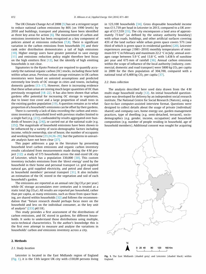
Fig. 1. The East Midlands (shaded grey) and Leicester (shaded black) withinEngland.
2. Methods
2.1. Study location
Leicester is located in the East Midlands region of England(Fig. 1), it is the 13th largest UK city with c330,00 persons living
in 123,100 households [34]. Gross disposable household incomewas £11,739 per head in Leicester in 2013, compared to a UK aver-age of £17,559 [35]. The city encompasses a land area of approxi-mately 73 km2 (as defined by the unitary authority boundary)with urban roads, buildings, and other artificial surfaces covering43% of the land surface while urban green space covers 57% (onethird of which is green space in residential gardens) [20]. Leicesterexperiences average (1981–2010) monthly temperatures of mini-mum 0.9 �C in February and maximum 22.2 �C in July; annual aver-ages range between 5.9 �C and 13.8 �C, with 1,438 h of sunshineper year and 675 mm of rainfall [36]. Annual carbon emissionswithin the scope of influence of the local authority (industry, com-mercial, domestic and road transport) were 5800 kg CO2 per capitain 2009 for the then population of 304,700, compared with anational total of 6,400 kg CO2 per capita [37].
2.2. Data collection
The analysis described here used data drawn from the 4 Mmulti-stage household study [12]. An initial household question-naire was developed for delivery by an independent social researchinstitute, The National Centre for Social Research (Natcen), using aface-to-face computer-assisted interview format. Questions weredesigned to collect details about the usage of private (individual/shared) and company cars, home energy use, garden managementpractices, type of dwelling (e.g. semi-detached, terraced), socio-demographics (e.g. gender, income, occupation) and householdcomposition (e.g. number of people residing in household, age ofhousehold members). Additional consent was sought for acquiring
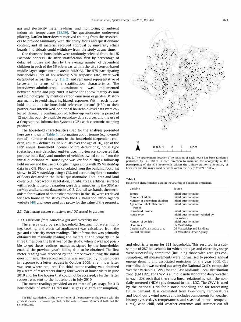
Fig. 2. The approximate location (The location of each house has been randomlyperturbed by +/� 100 m in each direction to maintain the anonymity of theparticipants) of the 575 households within the Unitary Authority Boundary ofLeicester and the major road network within the city (52�380N, 1�080W).
Table 1Household characteristics used in the analysis of household emissions.
Variable Source
Tenure Initial questionnaireNumber of adults Initial questionnaireNumber of dependent children Initial questionnaireAge of Household Reference
PersonInitial questionnaire
Household income Initial questionnaireHouse type Initial questionnaire- verified by
researchersNumber of vehicles Initial questionnaireFloor area OS MasterMapGarden artificial surface area OS MasterMap and LandbaseCouncil tax band UK Valuation Office Agency
D. Allinson et al. / Applied Energy 164 (2016) 871–881 873
gas and electricity meter readings, and monitoring of ambientindoor air temperature [38,39]. The questionnaire underwentpiloting, NatCen interviewers received training from the research-ers to provide familiarity with the study focus and questionnairecontent, and all material received approval by university ethicsboards. Individuals could withdraw from the study at any time.
One thousand households were randomly selected from the UKPostcode Address File after stratification, first by percentage ofdetached houses and then by the average number of dependentchildren in each of the 36 sub-areas within the city (census-basedmiddle layer super output areas; MLSOA). The 575 participatinghouseholds (0.5% of households; 57% response rate) were welldistributed across the city (Fig. 2) and remained representative ofLeicester in terms of the stratification characteristics. Theinterviewer-administered questionnaire was implementedbetween March and July 2009. It lasted for approximately 45 minand did not explicitly mention carbon emissions or garden OC stor-age,mainly to avoid triggeringbiased responses.Within eachhouse-hold one adult (the household reference person1 (HRP) or theirpartner) was interviewed. Additional household-level data were col-lected through a combination of: follow-up visits over a period of12 months, publicly available secondary data sources, and the use ofa Geographical Information Systems (GIS) with electronic mappingproducts.
The household characteristics used for the analyses presentedhere are shown in Table 1. Information about tenure (e.g. owned/rented), number of occupants in the household (dependent chil-dren, adults – defined as individuals over the age of 16), age of theHRP, annual household income (before deductions), house type(detached, semi-detached, end-terrace, mid-terrace, converted flat,purpose built flat), and number of vehicles owned came from theinitial questionnaire. House type was verified during a follow-upfield survey and the use of Google images alongwith OSMasterMapdata in a GIS. Floor area was calculated from the building footprintshown in OSMasterMap using a GIS, and accounting for the numberof floors declared in the initial questionnaire. Total area and landcover (e.g. herbaceous vegetation, shrubs, trees, artificial surface)within each household’s gardenwere determinedusing theOSMas-terMap and Landbase datasets in a GIS. Council tax bands, themech-anism for taxation of domestic properties in the UK, were retrievedfor each house in the study from the UK Valuation Office Agencywebsite [40] and were used as a proxy for the value of the property.
2.3. Calculating carbon emissions and OC stored in gardens
2.3.1. Emissions from household gas and electricity useThe energy used by each household (heating, hot water, light-
ing, cooking, and electrical appliances) was calculated from thegas and electricity meter readings. This information was primarilyobtained by manually reading the meters at the property up tothree times over the first year of the study; when it was not possi-ble to get these readings, mandates signed by the householderenabled the previous year’s billing data to be obtained. The firstmeter reading was recorded by the interviewer during the initialquestionnaire. The second reading was recorded by householdersin response to a letter request in October 2009; a reminder letterwas sent where required. The third meter reading was obtainedby a team of researchers during four weeks of house visits in June2010 and, for the houses that could not be accessed, a further letterrequest was sent to the households in July 2010.
The meter readings provided an estimate of gas usage for 313households, of which 11 did not use gas (i.e. zero consumption),
1 The HRP was defined as the owner/renter of the property, or the person with thegreatest income if co-owned/rented, or the oldest co-owner/renter if both had thesame income.
and electricity usage for 321 households. This resulted in a sub-sample of 287 households for which both gas and electricity usagewere successfully computed (including those with zero gas con-sumption). All measurements were normalised to produce annualenergy demand and associated emissions for the year 2009. Gasnormalisation was carried out using the National Grid’s ‘compositeweather variable’ (CWV) for the East Midlands ‘local distributionzone’ (EM LDZ). The CWV is a unique indicator of the daily weatherin each LDZ such that there is a linear relationship with the non-daily metered (NDM) gas demand in that LDZ. The CWV is usedby the National Grid for historic modelling and for forecastingfuture demand. It is calculated from two-hourly temperaturesand four-hourly wind speeds and includes components for weatherhistory (yesterday’s temperatures and seasonal normal tempera-tures), wind chill, cold weather extremes and summer cut off
874 D. Allinson et al. / Applied Energy 164 (2016) 871–881
[41]. Historic daily values for the CWV and NDM gas demand weredownloaded from the National Grid’s website [42]. For electricityconsumption the results were scaled linearly to 365 days. Finally,annual energy consumption was converted to CO2e emissionsusing conversion factors of 0.184 kg CO2e per kW h of natural gasand 0.544 kg CO2e per kW h of grid electricity [43].
2.3.2. Emissions from household personal transport useThe carbon emissions from personal transport were calculated
from responses to questions in the initial household questionnairethat identified the vehicle specification and usage for up to fivevehicles per household. Vehicle specification included make,model, engine size, age, and fuel type. Usage included the occu-pancy and frequency for journeys that were split into the followingcategories: very short (0–3 miles), short (3–8 miles), medium (8–50 miles) and long (more than 50 miles). Those responses withincomplete car specifications (n = 9) were replaced with an ‘aver-age car’ based on the UK vehicle licensing statistics for passengercars [44].
These data were used to calculate ‘ultimate’ carbon emissionsfrom published average speed emission factors from road vehicles[45] for typical journeys on urban roads in the UK (speed limit of30 mph (48.28 km/h)). The premise of this calculation is that allthe carbon in the fuel will ultimately produce CO2 in the atmo-sphere [46]. For consistency, the estimated carbon emissions wereconverted into CO2e based on the additional emissions of CH4 andN2O assumed for the 2009 vehicle fleet [47]. The calculationaccounted for cold starts in winter months which significantlyincrease carbon emissions for the short and very short journeys;these additional emissions were estimated using the assumptionsin the EXEMPT (Excess EMissions Planning Tool) model [48]. Thismodel overcomes some of the limitations of the TRAMAQ3 coldstart emission model [49] by including the changes in emissionsstandard from Euro 2 to Euro 4 vehicles. Cold start emissions weredirectly output as CO2e.
2.3.3. OC stored in household gardensTo estimate the OC stored in each household’s garden, 50 roads
across the city of Leicester were randomly selected in a GIS. Eachroad was visited and permission to sample within one gardenwas sought whenever there were houses in that road. Samplingincluded a survey of the vegetation in the entire back garden ofthe property. All tree species were identified and tree height anddiameter at breast height (DBH), 1.3 m, were recorded (see Davieset al. [19] for detailed methodology).
Within each garden, soils were sampled in the dominant vege-tation cover types, specifically herbaceous vegetation (predomi-nantly garden lawns) and from beneath shrubs and/or trees.Replicate soil samples were taken, to a depth of 21 cm, using a spe-cialist corer designed to take undisturbed samples (see Edmondsonet al. [20,50] for detailed methodology). Soil samples were dried at105 �C for 24 h, weighed, homogenised using a ball mill, and thenpassed through a 1 mm sieve. Fine earth soil bulk density (BD) wascalculated after removing the dry weight of any matter greaterthan 1 mm. Homogenised soils were analysed in duplicate for totalcarbon in an elemental analyser (Vario EL Cube, Elementar, Hanau,Germany). Soil organic carbon (SOC) density was calculated foreach individual soil sample using OC concentration and soil den-sity, taking into account the mass of the >1 mm fraction discardedafter milling. The figures used for SOC storage in domestic gardensbetween 0 and 21 cm depth were measured and between 21 and100 cm were modelled based on a negative exponential relation-ship derived from 25 samples to 1 m depth taken from across thecity. SOC storage was reported to 100 cm, as this is the standarddepth used to estimate SOC stock in the national inventory [13].
The detailed garden vegetation and soil surveys were used toderive mean figures for gardens across the city of Leicester, interms of the mass of carbon per unit land area, of: 0.79 kg/m2 forabove-ground OC; and 27.1 kg/m2 or 20.2 kg/m2 for soil OCbeneath trees and shrubs or herbaceous vegetation respectively.Of the 575 households that participated in the initial householdquestionnaire, 469 had gardens. The location of each one was iden-tified in a GIS and the garden boundaries were determined usingthe Ordnance Survey MasterMap dataset. Within each individualgarden, land cover classes were defined using the Landbase dataset(e.g. herbaceous vegetation, tree, shrub, artificial surface). The cor-responding areas within each garden were scaled up to estimatethe garden OC storage at the individual household level. Total OCstored in gardens was calculated as the sum of soil and above-ground OC and converted to kg CO2e.
A simple tree planting model, modified from McHugh et al. [51]was applied to those households with gardens (n = 469) to estimatetheir potential for reducing emissionsby the sequestration of carboninto biomass as OC. It was assumed that trees could only be ‘planted’in herbaceous vegetation (e.g. lawns, flowerbeds), and not in exist-ing patches of trees and shrubs or artificial surfaces (e.g. patios,driveways). The species in the domestic garden tree population inLeicester were determined in a previous survey [19] and split intosmall trees (mature canopy cover 17 m2) and large trees (maturecanopy cover 68 m2) [52]. The LandBase GIS dataset provided infor-mation onherbaceous vegetation patch sizewithin households’ gar-dens, so that treeswere only ‘planted’ in patches that exceeded theirmature canopy cover. Large trees were ‘planted’ in preference tosmall trees whenever patch size allowed as they are ultimately cap-able of storing considerably more OC [19,53]. Small trees were‘planted’ in the remaining available space (i.e. where patch sizeexceeded 17 m2). The subsequent growth of the virtual trees wasmodelled for 25 years, using the linear growth functions and bio-mass calculated using allometric equations described by McHughet al. [51]. Total biomass was then divided by 25 to give an averageannual CO2 sequestration rate over the course of the 25 year growthperiod. No account was made of the emissions from any gardenmaintenance activities that might be carried out by the households.
2.4. Data analysis
Descriptive statistics were used to analyse the distribution ofthe carbon emissions from household’s use of gas, electricity, andpersonal transport, as well as the combined total emissions andthe OC stored in gardens. The households were then ranked bytheir combined total emissions and divided by the tertiles intolow, medium and high groups. This followed a similar approachto the way that others have classified dwellings based on energyuse [54,55].
In the next step, the relative contributions that gas, electricityand transport emissions made to each household’s combined totalemissions was calculated. These were then compared across thehigh, medium and low total emissions groups to identify if the pro-portions remained consistent. The results from the tree plantingmodel were used to calculate the potential contribution of carbonsequestration to the reduction of total emissions for households inthe high, medium and low groups.
The classification of households by combined total emissionswas contrasted with how they would be classified by their gasemissions, electricity emissions, transport emissions and OC storedin the gardens. This was done to identify if classifying householdsinto the high group by one component of the total emissions, or byOC stored in gardens, would be a reasonable proxy for identifyingthose households in the high combined total emissions group. Con-fusion matrices were used to calculate the number of true positives(TP), true negatives (TN), false positives (FP), false negatives (FN),
D. Allinson et al. / Applied Energy 164 (2016) 871–881 875
true positive rate, false positive rate, and accuracy; following themethod described in the literature [56]. For example, for gas emis-sions: TP is the number of households that are in the high group forgas emissions and also in the high group for combined total emis-sions, TN is the number of households that are not in the highgroup for gas emissions and also not in the high group for totalemissions, FP is the number of households that are in the highgroup for gas emissions but not in the high group for total emis-sions, and FN is the number of households that are not in the highgroup for gas emissions but are in the high group for total emis-sions. True positive rate is the fraction of positives that are cor-rectly classified, false positive rate is the fraction of non-positivesthat are misclassified as positives, and accuracy is the proportionof the entire sample that are either TP or TN.
Exploratory model building was undertaken using multiple lin-ear regressions to examine the relationship between emissions andstorage (as outcome variables) and household characteristics (aspredictor variables). Stepwise regression was used in order to iden-tify characteristics that significantly predicted each outcome vari-able. For this purpose the categorical variables were transformedinto a single continuous variable: predictor that described housetype was recoded to create Number of Exposed Walls; householdincome categories were transformed by taking the midpoint ofeach income category (all categories had a lower and upper limit)and rounding up to the nearest integer thereby assigning eachhousehold a ‘Single Income Value’ [57].
Moderate to strong positive correlations existed among thenumber of exposed walls and floor area, council tax band and totalamount of artificial surface (ranging between rs = .451 to rs = .663).An additional strong positive relationship existed between incomeand number of vehicles in the household (rs = .512). As none of thecorrelations were above 0.7, all ten potential predictor variableswere included in an initial stepwise regression. The resulting setof statistically significant variables was examined both statisticallyand for plausibility (based on the authors’ conceptual and empiri-cal knowledge of the outcome variables); the final model was gen-erated from this reduced set of predictors entering all variables atthe same time (Enter method).
Regression models were constructed in SPSS version 20 [58];separate regression analyses were run for each outcome variable.The residual plots from the final regression models were analysedto determine how closely these followed a normal distribution.Where residuals showed large deviations from normality, transfor-mations were applied to the outcome variable, firstly by taking thesquare root, and then through a logarithmic transformation. Thetransformation which provided closest behaviour to normalitywas used in the final results: a natural log transformation fortransport emissions, garden storage and combined total emissions;and a square root transformation for electricity emissions [59].Significance levels were set at p < 0.05.
Table 2Results for household’s carbon emissions (gas, electricity, transport and the combined tot
Emissions, kg CO2e per annum in 2009
Gas Electricity
n* 313 281 321 281Median 2689 2687 1748 1746Meany 2909 2936 2105 2106Interquartile range 1928 1989 1480 1474Minimum 0 0 141 141Maximum 11,230 11,230 13,919 13,919Skew 0.89 0.97 2.82 3.02Kurtosis 2.38 2.63 15.13 17.04
* Figures in italics are for n = 281, i.e. those houses with results for gas, electricity andy Data are not normally distributed, but the mean is reported for comparison with othe
+ Garden OC storage figures are not annual emissions.
3. Results
3.1. Carbon emissions and OC stored in gardens
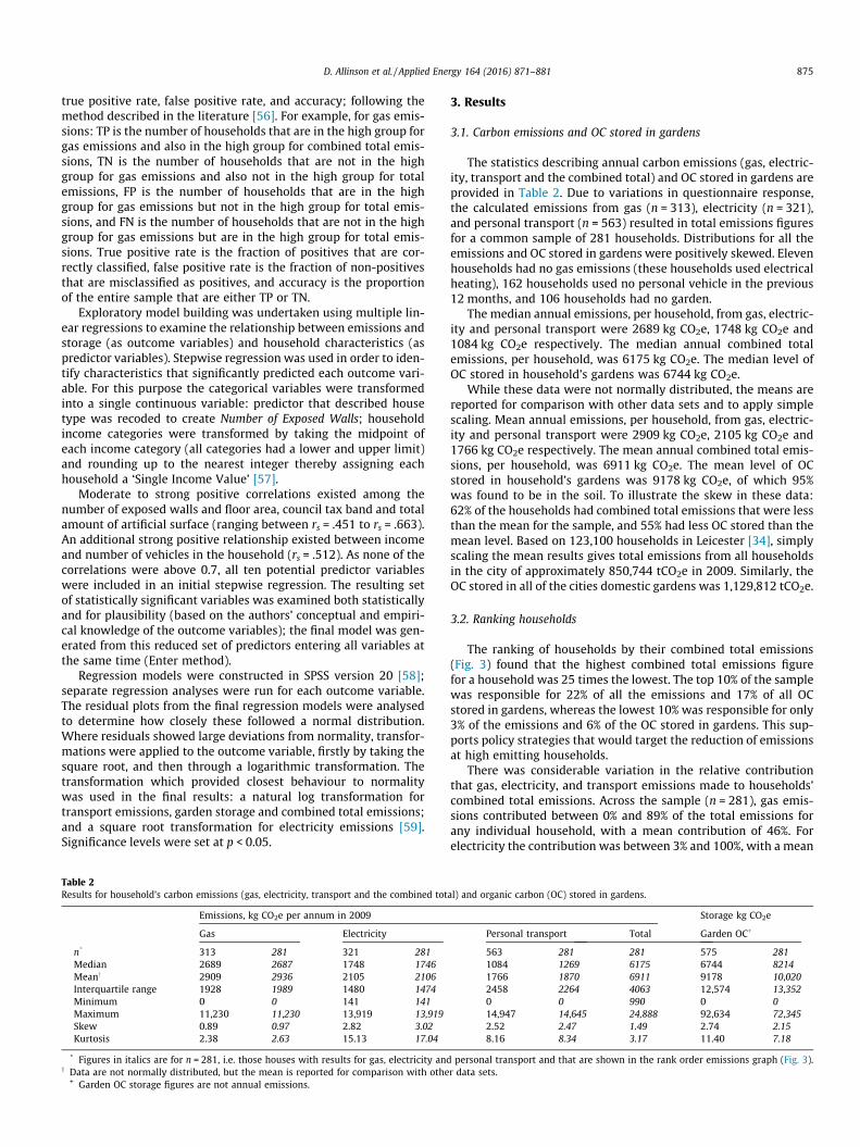
The statistics describing annual carbon emissions (gas, electric-ity, transport and the combined total) and OC stored in gardens areprovided in Table 2. Due to variations in questionnaire response,the calculated emissions from gas (n = 313), electricity (n = 321),and personal transport (n = 563) resulted in total emissions figuresfor a common sample of 281 households. Distributions for all theemissions and OC stored in gardens were positively skewed. Elevenhouseholds had no gas emissions (these households used electricalheating), 162 households used no personal vehicle in the previous12 months, and 106 households had no garden.
The median annual emissions, per household, from gas, electric-ity and personal transport were 2689 kg CO2e, 1748 kg CO2e and1084 kg CO2e respectively. The median annual combined totalemissions, per household, was 6175 kg CO2e. The median level ofOC stored in household’s gardens was 6744 kg CO2e.
While these data were not normally distributed, the means arereported for comparison with other data sets and to apply simplescaling. Mean annual emissions, per household, from gas, electric-ity and personal transport were 2909 kg CO2e, 2105 kg CO2e and1766 kg CO2e respectively. The mean annual combined total emis-sions, per household, was 6911 kg CO2e. The mean level of OCstored in household’s gardens was 9178 kg CO2e, of which 95%was found to be in the soil. To illustrate the skew in these data:62% of the households had combined total emissions that were lessthan the mean for the sample, and 55% had less OC stored than themean level. Based on 123,100 households in Leicester [34], simplyscaling the mean results gives total emissions from all householdsin the city of approximately 850,744 tCO2e in 2009. Similarly, theOC stored in all of the cities domestic gardens was 1,129,812 tCO2e.
3.2. Ranking households
The ranking of households by their combined total emissions(Fig. 3) found that the highest combined total emissions figurefor a household was 25 times the lowest. The top 10% of the samplewas responsible for 22% of all the emissions and 17% of all OCstored in gardens, whereas the lowest 10% was responsible for only3% of the emissions and 6% of the OC stored in gardens. This sup-ports policy strategies that would target the reduction of emissionsat high emitting households.
There was considerable variation in the relative contributionthat gas, electricity, and transport emissions made to households’combined total emissions. Across the sample (n = 281), gas emis-sions contributed between 0% and 89% of the total emissions forany individual household, with a mean contribution of 46%. Forelectricity the contribution was between 3% and 100%, with a mean
al) and organic carbon (OC) stored in gardens.
Storage kg CO2e
Personal transport Total Garden OC+
563 281 281 575 2811084 1269 6175 6744 82141766 1870 6911 9178 10,0202458 2264 4063 12,574 13,3520 0 990 0 014,947 14,645 24,888 92,634 72,3452.52 2.47 1.49 2.74 2.158.16 8.34 3.17 11.40 7.18
personal transport and that are shown in the rank order emissions graph (Fig. 3).r data sets.
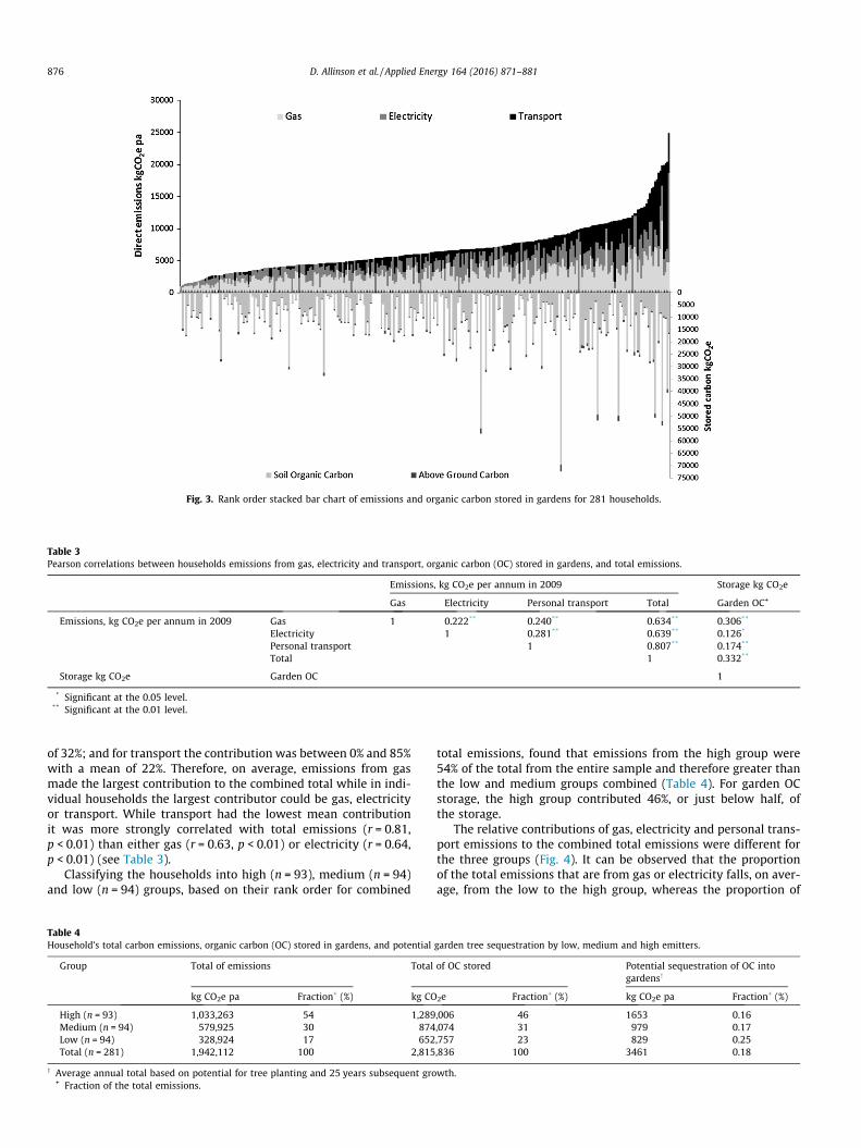
Fig. 3. Rank order stacked bar chart of emissions and organic carbon stored in gardens for 281 households.
Table 3Pearson correlations between households emissions from gas, electricity and transport, organic carbon (OC) stored in gardens, and total emissions.
Emissions, kg CO2e per annum in 2009 Storage kg CO2e
Gas Electricity Personal transport Total Garden OC+
Emissions, kg CO2e per annum in 2009 Gas 1 0.222** 0.240** 0.634** 0.306**
Electricity 1 0.281** 0.639** 0.126*
Personal transport 1 0.807** 0.174**
Total 1 0.332**
Storage kg CO2e Garden OC 1
* Significant at the 0.05 level.** Significant at the 0.01 level.
876 D. Allinson et al. / Applied Energy 164 (2016) 871–881
of 32%; and for transport the contribution was between 0% and 85%with a mean of 22%. Therefore, on average, emissions from gasmade the largest contribution to the combined total while in indi-vidual households the largest contributor could be gas, electricityor transport. While transport had the lowest mean contributionit was more strongly correlated with total emissions (r = 0.81,p < 0.01) than either gas (r = 0.63, p < 0.01) or electricity (r = 0.64,p < 0.01) (see Table 3).
Classifying the households into high (n = 93), medium (n = 94)and low (n = 94) groups, based on their rank order for combined
Table 4Household’s total carbon emissions, organic carbon (OC) stored in gardens, and potential
Group Total of emissions Total
kg CO2e pa Fraction+ (%) kg CO
High (n = 93) 1,033,263 54 1,289Medium (n = 94) 579,925 30 874Low (n = 94) 328,924 17 652Total (n = 281) 1,942,112 100 2,815
y Average annual total based on potential for tree planting and 25 years subsequent gro+ Fraction of the total emissions.
total emissions, found that emissions from the high group were54% of the total from the entire sample and therefore greater thanthe low and medium groups combined (Table 4). For garden OCstorage, the high group contributed 46%, or just below half, ofthe storage.
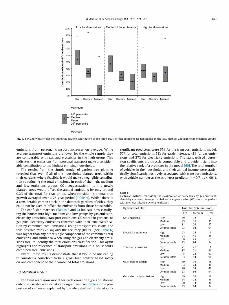
The relative contributions of gas, electricity and personal trans-port emissions to the combined total emissions were different forthe three groups (Fig. 4). It can be observed that the proportionof the total emissions that are from gas or electricity falls, on aver-age, from the low to the high group, whereas the proportion of
garden tree sequestration by low, medium and high emitters.
of OC stored Potential sequestration of OC intogardensy
2e Fraction+ (%) kg CO2e pa Fraction+ (%)
,006 46 1653 0.16,074 31 979 0.17,757 23 829 0.25,836 100 3461 0.18
wth.
Maximum
75th percentileMedianMean25th percentile
Minimum
0%
10%
20%
30%
40%
50%
60%
70%
80%
90%
100%
Gas Electricity Transport Gas Electricity Transport Gas Electricity Transport
Cont
ribu�
on to
hou
seho
ld's
tota
l em
issi
ons
Low total emissions Medium total emissions High total emissions
Fig. 4. Box and whisker plot indicating the relative contribution of the three areas of total emissions for households in the low, medium and high total emissions groups.
Table 5Confusion matrices contrasting the classification of households by gas emissions,electricity emissions, transport emissions or organic carbon (OC) stored in gardenswith their classification by total emissions.
Hypothesised class True class (total emissions)
High Medium Low
Gas emissions High 59 32 2Medium 23 36 35Low 11 26 57Column totals 93 94 94
Electricity emissions High 63 24 6Medium 24 45 25Low 6 25 63Column totals 93 94 94
Transport emissions High 71 21 1Medium 17 51 26Low 5 22 67Column totals 93 94 94
OC stored in garden High 39 36 18
D. Allinson et al. / Applied Energy 164 (2016) 871–881 877
emissions from personal transport increases on average. Whileaverage transport emissions are lower for the whole sample theyare comparable with gas and electricity in the high group. Thisindicates that emissions from personal transport make a consider-able contribution to the highest emitting households.
The results from the simple model of garden tree plantingrevealed that even if all of the households planted trees withintheir gardens, where feasible, it would make a negligible contribu-tion to reducing the total emissions. In each of the high, mediumand low emissions groups, CO2 sequestration into the newlyplanted trees would offset the annual emissions by only around0.2% of the total for that group, when considering annual treegrowth averaged over a 25-year period (Table 4). Whilst there isa considerable carbon stock in the domestic gardens of cities, theycould not be used to offset the emissions from those households.
The confusion matrices (Tables 5 and 6) indicate how classify-ing the houses into high, medium and low groups by gas emission,electricity emissions, transport emissions, OC stored in gardens, orgas plus electricity emissions contrasts with their true classifica-tion by combined total emissions. Using transport emissions, thetrue positive rate (76.3%) and the accuracy (84.3%) (see Table 6)was higher than any other single component of the combined totalemissions, and similar to when using the gas and electricity emis-sions total to identify the total emissions classification. This againhighlights the relevance of transport emissions to a household’scombined total emissions.
Overall these results demonstrate that it would be misleadingto consider a household to be a gross high emitter based solelyon one component of their combined total emissions.
Medium 34 24 36Low 20 34 40Column totals 93 94 94
Gas + electricity emissions High 39 36 18Medium 34 24 36Low 20 34 40Column totals 93 94 94
3.3. Statistical models
The final regression model for each emission type and storageoutcome variable was statistically significant (see Table 7). The pro-portion of variances explained by the identified set of statistically
significant predictors were 67% for the transport emissions model,57% for total emissions, 51% for garden storage, 41% for gas emis-sions and 27% for electricity emissions. The standardised regres-sion coefficients are directly comparable and provide insight intothe relative rank of a predictor in the model [60]. The total numberof vehicles in the households and their annual income were statis-tically significantly positively associated with transport emissions,with vehicle number as the strongest predictor (b = 0.71, p < .001).
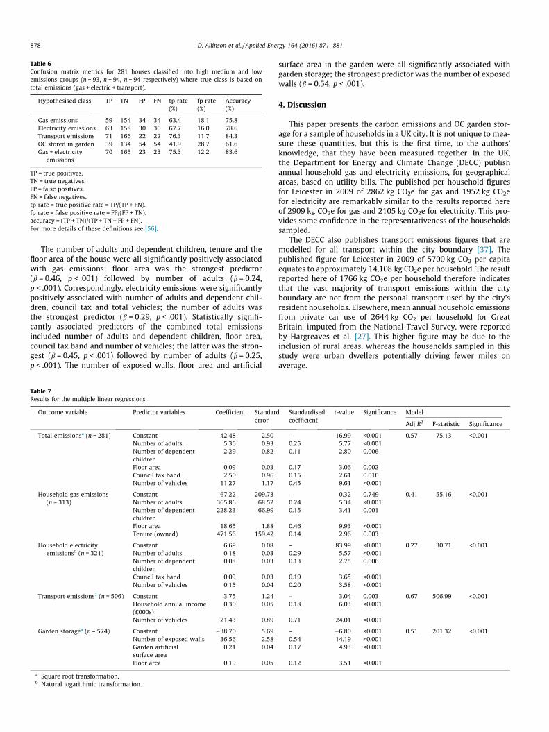
Table 6Confusion matrix metrics for 281 houses classified into high medium and lowemissions groups (n = 93, n = 94, n = 94 respectively) where true class is based ontotal emissions (gas + electric + transport).
Hypothesised class TP TN FP FN tp rate(%)
fp rate(%)
Accuracy(%)
Gas emissions 59 154 34 34 63.4 18.1 75.8Electricity emissions 63 158 30 30 67.7 16.0 78.6Transport emissions 71 166 22 22 76.3 11.7 84.3OC stored in garden 39 134 54 54 41.9 28.7 61.6Gas + electricity
emissions70 165 23 23 75.3 12.2 83.6
TP = true positives.TN = true negatives.FP = false positives.FN = false negatives.tp rate = true positive rate = TP/(TP + FN).fp rate = false positive rate = FP/(FP + TN).accuracy = (TP + TN)/(TP + TN + FP + FN).For more details of these definitions see [56].
878 D. Allinson et al. / Applied Energy 164 (2016) 871–881
The number of adults and dependent children, tenure and thefloor area of the house were all significantly positively associatedwith gas emissions; floor area was the strongest predictor(b = 0.46, p < .001) followed by number of adults (b = 0.24,p < .001). Correspondingly, electricity emissions were significantlypositively associated with number of adults and dependent chil-dren, council tax and total vehicles; the number of adults wasthe strongest predictor (b = 0.29, p < .001). Statistically signifi-cantly associated predictors of the combined total emissionsincluded number of adults and dependent children, floor area,council tax band and number of vehicles; the latter was the stron-gest (b = 0.45, p < .001) followed by number of adults (b = 0.25,p < .001). The number of exposed walls, floor area and artificial
Table 7Results for the multiple linear regressions.
Outcome variable Predictor variables Coefficient Standarderror
Total emissionsa (n = 281) Constant 42.48 2.50Number of adults 5.36 0.93Number of dependentchildren
2.29 0.82
Floor area 0.09 0.03Council tax band 2.50 0.96Number of vehicles 11.27 1.17
Household gas emissions(n = 313)
Constant 67.22 209.73Number of adults 365.86 68.52Number of dependentchildren
228.23 66.99
Floor area 18.65 1.88Tenure (owned) 471.56 159.42
Household electricityemissionsb (n = 321)
Constant 6.69 0.08Number of adults 0.18 0.03Number of dependentchildren
0.08 0.03
Council tax band 0.09 0.03Number of vehicles 0.15 0.04
Transport emissionsa (n = 506) Constant 3.75 1.24Household annual income(£000s)
0.30 0.05
Number of vehicles 21.43 0.89
Garden storagea (n = 574) Constant �38.70 5.69Number of exposed walls 36.56 2.58Garden artificialsurface area
0.21 0.04
Floor area 0.19 0.05
a Square root transformation.b Natural logarithmic transformation.
surface area in the garden were all significantly associated withgarden storage; the strongest predictor was the number of exposedwalls (b = 0.54, p < .001).
4. Discussion
This paper presents the carbon emissions and OC garden stor-age for a sample of households in a UK city. It is not unique to mea-sure these quantities, but this is the first time, to the authors’knowledge, that they have been measured together. In the UK,the Department for Energy and Climate Change (DECC) publishannual household gas and electricity emissions, for geographicalareas, based on utility bills. The published per household figuresfor Leicester in 2009 of 2862 kg CO2e for gas and 1952 kg CO2efor electricity are remarkably similar to the results reported hereof 2909 kg CO2e for gas and 2105 kg CO2e for electricity. This pro-vides some confidence in the representativeness of the householdssampled.
The DECC also publishes transport emissions figures that aremodelled for all transport within the city boundary [37]. Thepublished figure for Leicester in 2009 of 5700 kg CO2 per capitaequates to approximately 14,108 kg CO2e per household. The resultreported here of 1766 kg CO2e per household therefore indicatesthat the vast majority of transport emissions within the cityboundary are not from the personal transport used by the city’sresident households. Elsewhere, mean annual household emissionsfrom private car use of 2644 kg CO2 per household for GreatBritain, imputed from the National Travel Survey, were reportedby Hargreaves et al. [27]. This higher figure may be due to theinclusion of rural areas, whereas the households sampled in thisstudy were urban dwellers potentially driving fewer miles onaverage.
Standardisedcoefficient
t-value Significance Model
Adj R2 F-statistic Significance
– 16.99 <0.001 0.57 75.13 <0.0010.25 5.77 <0.0010.11 2.80 0.006
0.17 3.06 0.0020.15 2.61 0.0100.45 9.61 <0.001
– 0.32 0.749 0.41 55.16 <0.0010.24 5.34 <0.0010.15 3.41 0.001
0.46 9.93 <0.0010.14 2.96 0.003
– 83.99 <0.001 0.27 30.71 <0.0010.29 5.57 <0.0010.13 2.75 0.006
0.19 3.65 <0.0010.20 3.58 <0.001
– 3.04 0.003 0.67 506.99 <0.0010.18 6.03 <0.001
0.71 24.01 <0.001
– �6.80 <0.001 0.51 201.32 <0.0010.54 14.19 <0.0010.17 4.93 <0.001
0.12 3.51 <0.001
D. Allinson et al. / Applied Energy 164 (2016) 871–881 879
The mean OC storage, of 9,178 kg CO2e per household garden, ismore than three times higher than currently assumed in urbanareas in the English national OC inventory [13]. This demonstratesthat small, individually managed and discrete patches of greenspaces can enhance citywide OC stocks. The result is commensu-rate with other recent findings on OC storage in urban gardens asestimated for all gardens across the city [20] and confirms the rep-resentativeness of the 575 gardens in this study.
While mean values are used for comparison purposes above,our results show that household emissions are not normally dis-tributed and that the mean is higher than the corresponding med-ian for the emissions individually (gas, electricity, and personaltransport) as well as for the OC stored in gardens. The highestone-third of the households had greater total emissions than theother two-thirds combined. Emissions reduction policies could betargeted directly at this high total emissions group, but it may bedifficult to identify them from averaged results. Therefore it is sug-gested that the distributions of emissions figures be reportedalongside averaged values in published aggregate emissions statis-tics, such as sub-national consumption data [61].
The lowest emitting household in the study comprised a singleworking adult, in a small house and with no personal transport. Itis possible that they may have spent periods of time away fromhome over the period of the study. The highest emitting householdcomprised three adults in a large house with two cars and a partic-ularly high number of short and very short vehicle journeys, plushigh electricity usage. For the households in-between, the relativecontributions of gas, electricity, and personal transport to the totalcarbon emissions varied widely. Emissions from gas were highestacross the sample, and highest on average in the high total emis-sions group. However, the average contribution (mean ratio of ahousehold’s gas emissions to their total emissions) was lower inthe high group compared to the other two groups. In fact, withinthe high group the mean contributions of gas, electricity and per-sonal transport to total emissions were relatively similar. Addition-ally, the confusion matrices demonstrated that the highestemitting households can only be identified reliably from their totalemissions and not from any single component. Taken together,these findings substantiate the relevance of reporting total emis-sions figures that include transport emissions, alongside gas andelectricity emissions, in national statistics. Also, they highlight anew opportunity to target a single group of households in orderto tackle emissions from both the domestic and transport sectors.Viable technical solutions are readily available, if not easy toimplement, and include installing insulation and low carbon heat-ing systems into homes, and a mode shift to public transport.
The data presented for individual garden OC storage provideinsight into the contribution that individual houses and their asso-ciated gardens can make to the carbon budget of a city. The ratio ofthe total OC stored in a household’s gardens to their total annualemissions ranged from zero to 12.7, with a median value of 1.2and a mean of 1.7. Non-domestic urban greenspaces can be man-aged to offset a greater proportion of the CO2 emitted by house-holds than can domestic gardens, because of the potential todensely plant high yielding tree species such as willow and popularin short-rotation coppice. Over 25 years, the coppice can yield30 times more carbon sequestration into above-ground biomassper unit area than individual trees of the kinds found in gardens[51]. In Leicester, an area of 5.8 km2 was recently identified aspotentially suitable for short rotation coppice planting, and wasestimated to have the potential to sequester 71,800 tonnes ofcarbon in harvested biomass over 25 years [51]. Nonetheless, esti-mates of large amounts of carbon stored within gardens demon-strates the valuable service provided by these individual, discretepatches of urban greenspace. The findings highlight the role ofindividual households in maximising carbon storage potentials
by: increasing the greenspace cover and minimising the artificialsurface (e.g. paving or decking) within gardens; and managing gar-dens with minimal reliance on fossil fuel powered machinery.
For cities where residential green space is less common, similarOC storage densities can be provided by non-residential land, suchas urban parks [20]. The case for green roofs on building is lessclear, though. This study demonstrates that the majority of carbonis stored in the soils. Green roofs tend to be grown on lightweightsubstrates for obvious structural reasons. Furthermore, it has beenshown that trees account for the vast majority of above ground car-bon [19] while standard green roofs are based on herbaceous orlow-productivity succulent species like Sedum and only very rarelyare trees grown (and in these cases as pot-plants rather than inroof substrate). Even if we assume that green roofs would not bemown, and might hold a slightly greater above-ground biomassthan short-mown grass, the contribution of green roofs, both inaerial extent, and in above-ground biomass carbon, would meanthat they would be insignificant contributors to urban ecosystemcarbon stores.
The holistic consideration of households’ total emissions andgarden OC storage, as suggested in this paper, is logical as activitiesthat reduce emissions from one source may increase them inanother. For example, a household with electrical space heatingmay have high carbon emissions from electricity use, while thosefrom gas use are zero. A household member who worked fromhome may increase the emissions attributed to gas and electricity(for heating, lighting and appliance use within the house) but therecould be a consequential reduction in emissions from fuel useddriving their car to work. Using a car powered by electricity wouldremove the emissions attributed to petrol and diesel for personaltransport but increase household electricity emissions. Householdsmay pave their front garden to enable off road parking and increasevehicle ownership, while simultaneously reducing above groundOC storage in vegetation and opportunities for further sequestra-tion. In order to reduce the possibility of unintended consequences,and direct or indirect rebound effects, any emissions reduction pol-icy targeting the domestic sector should consider the conse-quences across a household’s entire emissions and OC storagebudget. National level data, of the type presented in this study,are needed to support such policy.
The statistical models showed that households with moreadults, more children, living in larger and more valuable houses,and owning more vehicles tend to have higher total emissions aswould be expected. Household’s annual income featured in thetransport model, along with vehicle ownership, as a strong predic-tor of transport emissions. More work is required to understandbetter what causes emissions in households with high total emis-sions, but these results indicate the predictive power of comple-mentary datasets.
This study achieved a more holistic evaluation by carrying outthe data collection, analysis and interpretation using methods froma number of academic disciplines including transport studies,building energy demand, ecology, and social sciences. Primary datacollection was supplemented with secondary data sets, includingcouncil tax band and electronic mapping products. Data collectionmechanisms such as these are not unique. For example, the EnglishHouse Condition Survey (a mainly technical study) and the Surveyof English Housing (a mainly social study) were joined to producethe English Housing Survey, part of the integrated household sur-vey [62]. Similarly the National Energy Efficiency Data-framework (NEED) [63] combines data from a number of sources,including gas and electricity billing data, and data held by the gov-ernment’s Valuation Office Agency, to produce an extremely valu-able resource for building energy research. These existing data setscould be augmented with new questions, or combined with exist-ing data sets, in order to include transport emissions and OC stored

880 D. Allinson et al. / Applied Energy 164 (2016) 871–881
in gardens. The UK Department for Transport’s Driver and VehicleLicensing Agency (DVLA) already has a database of car ownershipwhich could, for example, be added to NEED. In this way the costof providing nationally representative data sets that combine emis-sions and garden OC storage need not be prohibitively expensive.
5. Conclusions
An in-depth study of 575 households across the city of Leicesterin the UK was carried out in 2009 by a multidisciplinary team ofresearchers. Annual totals of households’ carbon emissions fromend-use energy demand were summed from: gas and electricitymeter readings and self-reported vehicle ownership and trips pat-terns. Carbon stored above ground in vegetation and in the soil ofthe gardens was estimated from the results of a unique field trial.Additional socio-demographic and descriptive data were collectedfrom the households and supplemented by secondary data sets.
Median annual household emissions from gas, electricity andpersonal transport were 2689 kg CO2e, 1748 kg CO2e and 1084 kgCO2e per household per year respectively. The median level of OCstored in household’s gardens was 6744 kg CO2e. The median ofthe total emissions was 6175 kg CO2e per household.
The overall carbon distribution patterns were skewed, with thehighest emitting third of the households being responsible formore than 50% of all emissions and around 50% of garden OC stor-age. The relative contribution of gas, electricity and personal trans-port emissions to the total was shown to vary from household tohousehold. Emissions from gas were dominant on average, butthe average contributions from gas, electricity and personal trans-port were similar in the highest emitting third of the households.There were large amounts of OC stored in households’ gardensbut the available potential for tree planting in gardens was esti-mated to provide annual emissions reductions of only 0.2% (basedon average sequestration over 25 years of growth in trees reflectingcurrent species composition in gardens and planted at low densityin spaces that would accommodate them at maturity). However,more work is needed to understand the causes and predictors ofemissions and this might fruitfully concentrate on the high emis-sions group of households.
The implications of these results for policies that aim to reducecarbon emissions from end-use energy demand in the domesticsector include
� It may be beneficial to target the top third of households bytotal emissions, as over half of the emissions are from thisgroup.
� Any policy targeting households with high carbon emissionsshould consider methods to reduce demand for gas, electricityand personal transport together.
� Emission reduction policies would benefit from geographicallydisaggregated national data sets that report the distributionsof emissions totals, as well as the distributions of their compo-nents: gas, electricity and personal transport.
� New data sets could be created by combining existing data anddata collection mechanisms, or new measurements made in arepresentative sample of households.
� Contemporaneous socio-demographic data for households arerequired to understand the predictors of emissions and thiscould be provided from existing secondary data.
It is also suggested that the considerable amounts of organiccarbon stored in household’s gardens should be protected.
These findings will be relevant in devising effective policyinstruments for combatting global city-scale green-house gasemissions from domestic end-use energy demand in response towarnings from the IPCC.
Acknowledgements
This work is supported by the EPSRC projects Measurement,Modelling, Mapping and Management 4M: An Evidence BasedMethodology for Understanding and Shrinking the Urban CarbonFootprint (grant reference EP/F007604/1) and Self ConservingUrbanEnvironments (SECURE, grant reference EP/I002154/1) fundedunder the SustainableUrbanEnvironments programme. Theuniver-sity partnerswere assisted by an advisory panel drawn fromUKcen-tral and local government, and UK and overseas industry andacademia. Katherine Irvine was partially supported by the ScottishGovernment’s Rural and Environment Science and AnalyticalServices Division (RESAS). Infoterra provided access to LandBase;MasterMap data were supplied by the Ordnance Survey.
References
[1] IPCC. Climate change 2014: synthesis report-headline statements from thesummary for policymakers. Intergovernmental panel on climate change; 2014.
[2] Yuan B, Ren S, Chen X. The effects of urbanization, consumption ratio andconsumption structure on residential indirect CO2 emissions in China: aregional comparative analysis. Appl Energy 2015;140:94–106. http://dx.doi.org/10.1016/j.apenergy.2014.11.047.
[3] International Energy Agency. World energy outlook 2008. OECD Publishing;2008. http://dx.doi.org/10.1787/weo-2005-en.
[4] Fang C, Wang S, Li G. Changing urban forms and carbon dioxide emissions inChina: a case study of 30 provincial capital cities. Appl Energy2015;158:519–31. http://dx.doi.org/10.1016/j.apenergy.2015.08.095.
[5] Britain Great. Climate change act 2008 c27. London: The Stationery Office;2008.
[6] Committee on Climate Change. How local authorities can reduce emissionsand manage climate risk; 2012.
[7] SalonD, Sperling D,Meier A,Murphy S, GorhamR, Barrett J. City carbon budgets:a proposal to align incentives for climate-friendly communities. Energy Policy2010;38:2032–41. http://dx.doi.org/10.1016/j.enpol.2009.12.005.
[8] Dixon T. Hotting up? An analysis of low carbon plans and strategies for UKcities: main findings, vol. 1. London: Royal Institution of Chartered Surveyors;2011.
[9] Thumin J, White V. Distributional impacts of personal carbon trading. Finalreport to the UK Department for Environment Food and Rural Affairs; 2008.
[10] Gough I, Abdallah S, Johnson V. The distribution of total greenhouse gasemissions by households in the UK, and some implications for social policy,vol. 2011; 2011.
[11] Firth SK, Lomas KJ, Wright aJ. Targeting household energy-efficiency measuresusing sensitivity analysis.. Build Res Inf 2010;38:25–41. http://dx.doi.org/10.1080/0961321090323670.
[12] Lomas KJ, Bell MC, Firth SK, Gaston KJ, Goodman P, Leake JR, et al. The carbonfootprint of UK cities 4M: measurement, modelling, mapping andmanagement ISOCARP Rev 06. Int Soc City Reg Planners; (2011).
[13] Bradley RI, Milne R, Bell J, Lilly a, Jordan C, Higgins a. A soil carbon and land usedatabase for the United Kingdom. Soil Use Manag 2005;21:363–9. http://dx.doi.org/10.1079/SUM2005351.
[14] Arrouays D, Deslais W, Badeau V. The carbon content of topsoil and itsgeographical distribution in France. Soil Use Manag 2001;17:7–11. http://dx.doi.org/10.1079/SUM200053.
[15] Milne R, Brown TA. Carbon in the vegetation and soils of great britain. JEnviron Manage 1997;49:413–33. http://dx.doi.org/10.1006/jema.1995.0118.
[16] Xu X, Liu W, Zhang C, Kiely G. Estimation of soil organic carbon stock and itsspatial distribution in the Republic of Ireland. Soil Use Manag2011;27:156–62. http://dx.doi.org/10.1111/j.1475-2743.2011.00342.x.
[17] Cruickshank M, Tomlinson RW, Devine PM, Milne R. Carbon in the soils andvegetation of Northern Ireland. Biol Environ Proc R Irish Acad 1998;98B:9–21.
[18] Pouyat RV, Yesilonis ID, Nowak DJ. Carbon storage by urban soils in the UnitedStates. J Environ Qual 2006;35:1566–75. http://dx.doi.org/10.2134/jeq2005.0215.
[19] Davies ZG, Edmondson JL, Heinemeyer A, Leake JR, Gaston KJ. Mapping anurban ecosystem service. quantifying above-ground carbon storage at a city-wide scale. J Appl Ecol 2011;48:1125–34. http://dx.doi.org/10.1111/j.1365-2664.2011.02021.x.
[20] Edmondson JL, Davies ZG, McHugh N, Gaston KJ, Leake JR. Organic carbonhidden in urban ecosystems. Sci Rep 2012;2:963. http://dx.doi.org/10.1038/srep00963.
[21] Edmondson JL, Davies ZG, McCormack Sa, Gaston KJ, Leake JR. Land-covereffects on soil organic carbon stocks in a European city. Sci Total Environ2014;472:444–53. http://dx.doi.org/10.1016/j.scitotenv.2013.11.025.
[22] Edmondson JL, Davies ZG, Gaston KJ, Leake JR. Urban cultivation in allotmentsmaintains soil qualities adversely affected by conventional agriculture. J ApplEcol 2014;51:880–9. http://dx.doi.org/10.1111/1365-2664.12254.
[23] Jones RV, Lomas KJ. Determinants of high electrical energy demand in UKhomes: socio-economic and dwelling characteristics. Energy Build2015;101:24–34. http://dx.doi.org/10.1016/j.enbuild.2015.04.052.

D. Allinson et al. / Applied Energy 164 (2016) 871–881 881
[24] Morris J, Allinson D, Harrison J, Lomas KJ. Benchmarking and tracking domesticgas and electricity consumption at the local authority level. Energy Effic 2015.http://dx.doi.org/10.1007/s12053-015-9393-8.
[25] Chitnis M, Hunt LC. What drives the change in UK household energyexpenditure and associated CO2 emissions? Implication and forecast to2020. Appl Energy 2012;94:202–14. http://dx.doi.org/10.1016/j.apenergy.2012.01.005.
[26] Baker KJ, Rylatt RM. Improving the prediction of UK domestic energy-demandusing annual consumption-data. Appl Energy 2008;85:475–82. http://dx.doi.org/10.1016/j.apenergy.2007.09.004.
[27] Hargreaves K, Preston I, White V. The distribution of household CO2 emissionsin Great Britain – updated version supplementary project paper no1. CentreSust Energy Joseph Rowntree Found 2013.
[28] Aydinalp-Koksal M, Ugursal VI. Comparison of neural network, conditionaldemand analysis, and engineering approaches for modeling end-use energyconsumption in the residential sector. Appl Energy 2008;85:271–96. http://dx.doi.org/10.1016/j.apenergy.2006.09.012.
[29] Büchs M, Schnepf SV. Who emits most? Associations between socio-economicfactors and UK households’ home energy, transport, indirect and total CO2
emissions. Ecol Econ 2013;90:114–23. http://dx.doi.org/10.1016/j.ecolecon.2013.03.007.
[30] Office for National Statistics. Key statistics for local authorities in England andWales, Table KS101EW 2011 census: usual resident population, localauthorities in England and wales; 2011.
[31] Weber C, Perrels A. Modelling lifestyle effects on energy demand and relatedemissions. Energy Policy 2000;28:549–66. http://dx.doi.org/10.1016/S0301-4215(00)00040-9.
[32] Druckman A, Jackson T. An exploration into the carbon footprint of UKhouseholds. Soc Res (New York); 2010. Resolve working paper 02–10.
[33] Hargreaves T, Nye M, Burgess J. Making energy visible: a qualitative field studyof how householders interact with feedback from smart energy monitors.Energy Policy 2010;38:6111–9. http://dx.doi.org/10.1016/j.enpol.2010.05.068.
[34] ONS. 2011 Census-first release of statistics: population and householdestimates for England and Wales; 2012. <http://www.ons.gov.uk/ons/guide-method/census/2011/census-data/2011-census-data/2011-first-release/index.html>.
[35] ONS. Regional gross disposable household income (GDHI), 1997–2013. Officefor National Statistics Statistical Bulletin; 2015.
[36] Met Office. Leicester climate; 2015. <http://www.metoffice.gov.uk/public/weather/climate/leicester> (accessed April 22, 2015).
[37] DECC. Carbon dioxide emissions within the scope of influence of localauthorities (previously NI 186); 2011. <http://www.decc.gov.uk/en/content/cms/statistics/local_auth/co2_las/co2_las.aspx>.
[38] Lomas KJ, Kane T. Summertime temperatures in 282 UK homes: thermalcomfort and overheating risk. In: Proc 7th Wind Conf Chang Context Comf anunpredictable world. London: Network for comfort and energy use inbuildings; 2012, p. 12–5.
[39] Kane T, Firth SK, Lomas KJ. How are UK homes heated? A city-wide, socio-technical survey and implications for energy modelling. Energy Build2015;86:817–32. http://dx.doi.org/10.1016/j.enbuild.2014.10.011.
[40] Valuation Office Agency. Search for your council tax band; 2012. <http://www.voa.gov.uk/cti/InitS.asp?lcn=0> (accessed May 31, 2012).
[41] National Grid. Gas demand forecasting methodology; 2007.[42] National Grid. Data item explorer; 2010. <http://marketinformation.natgrid.
co.uk/gas/DataItemExplorer.aspx> (accessed September 3, 2010).[43] Carbon Trust. Conversion factors: energy and carbon conversions 2009 update;
2009.[44] DfT. Vehicle licensing statistics 2010. London: Department for Transport;
2011.[45] Defra. Defra 2009 emission factors; 2009. <http://www.dft.gov.uk/
publications/road-vehicle-emission-factors-2009/> (accessed June 11, 2010).[46] CERC. EMIT atmospheric emissions inventory toolkit: user guide. Cambridge
Environmental Research Consultants; 2011.[47] AEA. Greenhouse gas inventories for England, Scotland, Wales and Northern
Ireland: 1990–2007. Appendix I: DA GHGI estimation methodology. UK: AEATechnology Plc; 2009.
[48] AEA. Cold start advanced – User guide. UK: AEA Technology Plc; 2008.[49] Boulter PG, Latham S. Emission factors 2009: Report 4 – a review of
methodologies for modelling cold-start emissions; TRL published projectreport: PPR357; 2009.
[50] Edmondson JL, Davies ZG, McCormack SA, Gaston KJ, Leake JR. Are soils inurban ecosystems compacted? A citywide analysis. Biol Lett 2011;7:771–4.http://dx.doi.org/10.1098/rsbl.2011.0260.
[51] McHugh N, Edmondson JL, Gaston KJ, Leake JR, O’Sullivan OS. Modelling short-rotation coppice and tree planting for urban carbon management – a citywideanalysis. J Appl Ecol 2015;52:1237–45. http://dx.doi.org/10.1111/1365-2664.12491.
[52] Wu C, Xiao Q, McPherson EG. A method for locating potential tree-plantingsites in urban areas: a case study of Los Angeles, USA. Urban Urban Green2008;7:65–76. http://dx.doi.org/10.1016/j.ufug.2008.01.002.
[53] Nowak DJ, Crane DE. Carbon storage and sequestration by urban trees in theUSA. Environ Pollut 2002;116:381–9.
[54] Firth S, Lomas K, Wright a, Wall R. Identifying trends in the use of domesticappliances from household electricity consumption measurements. EnergyBuild 2008;40:926–36. http://dx.doi.org/10.1016/j.enbuild.2007.07.005.
[55] Summerfield AJ, Pathan A, Lowe RJ, Oreszczyn T. Changes in energy demandfrom low-energy homes. Build Res Inf 2010;38:42–9. http://dx.doi.org/10.1080/09613210903262512.
[56] Fawcett T. An introduction to ROC analysis. Pattern Recognit Lett2006;27:861–74. http://dx.doi.org/10.1016/j.patrec.2005.10.010.
[57] Hout M. Getting the most out of the GSS income measures – GSSmethodological report 101; 2004.
[58] IBM. SPSS Statistics for windows, version 19.0; 2010.[59] Tabachnick BG, Fidel LS. Using multivariate statistics. 6th ed. Boston (MA,
USA): Allyn and Bacon; 2013.[60] Field A. Discovering statistics using SPSS. 3rd ed. London: Sage; 2007.[61] DECC. Sub-national energy consumption statistics – Department of Energy and
Climate Change; 2012. <http://www.decc.gov.uk/en/content/cms/statistics/energy_stats/regional/regional.aspx> (accessed December 4, 2012).
[62] ESDS. Integrated household survey – Economic and Social Data Services; n.d.<http://www.esds.ac.uk/government/ihs/> (accessed December 5, 2012).
[63] DECC. National energy efficiency data-framework (NEED); 2013. <https://www.gov.uk/government/collections/national-energy-efficiency-data-need-framework> (accessed December 22, 2014).