measurement and visualization of oscillatory flow in a

10th Pacific Symposium on Flow Visualization and Image Processing Naples, Italy, 15-18 June, 2015

Measurement and Visualization of Oscillatory Flow in a Thermoacoustic Engine

using PIV

Kazuto Kuzuu1,*, Shinya Hasegawa1

1Department of Prime Mover Engineering, Tokai University, Hiratsuka, Kanagawa, 2591292, Japan

*corresponding author: [email protected]

Abstract We conduct the experiment for a thermoacoustic phenomenon occurred in a thermoacoustic device, and investigate the effect of large displacement amplitudes on energy transfer efficiency. In the experiment, we first generate the thermoacoustic phenomenon with large displacement amplitude and measure the oscillatory flow induced by this phenomenon. Furthermore, we visualize the flow near the entrance/exit of the engine device. This device is composed of two heat exchangers (hot and cold) and a stack. From the experimental results, we confirm not only the vortex generation but also the disturbance within the device. Both of them can be regarded as non-linear phenomenon by large displacement amplitude. In the present study, we also carried out the CFD simulation in addition to the experiment. This is for obtaining the information of temperature distribution. Therefore, we first compare the velocity field of CFD with the experimental one and verify the CFD simulation. Then, we discuss the heat transfer within the engine. From these results, we make clear the effect of large displacement amplitude on temperature distribution of fluid in the engine. Finally, we calculate the acoustic power from both experimental and CFD results, and discuss the effect of temperature distribution on energy transfer efficiency. Keywords: thermoacoustic engine, PIV, CFD

1 Introduction

A thermoacoustic engine is expected as a system for recovering renewable heat energy. This engine has been studied extensively since Swift demonstrated an inexpensive prototype [1]. On the other hand, many basic theories have been suggested in the field of acoustics [2]-[8], and they are available for the development of this engine. However, both of those theories are based on the assumption of linear phenomena. For replying the requirement for higher performance of this engine, we have to understand the nonlinear phenomena occurred in the thermoacoustic engine. Especially, when considering energy efficiency of the engine, we have to estimate the temperature distribution within the engine. However, it is difficult to predict the actual fluid temperature distribution for oscillatory flow with large displacement amplitude, since this distribution might be affected by both of convection term in the stream wise and conduction term between wall and fluid. Thus, we have to solve the problem of heat transfer with large displacement amplitude so long as we pursue high performance on the thermoacoustic engine. With respect to the estimation of heat transfer of oscillatory flow inside the engine, some numerical approaches combined with the classical linear thermoacoustic theory are suggested [9][10]. In their studies, the heat transfer of oscillatory flow considering heat exchange between wall and fluid is discussed, and phase dependent heat transfer rates and Nusselt numbers are investigated. However, for the oscillatory flow with larger displacement amplitude, which can be occurred in the actual engine, we have to consider the interaction of heat transfers among the heat exchangers, the stack and the resonator, and the conventional approach cannot reproduce those interactions. In order to investigate the effect of large displacement of fluid motion on temperature distribution, the direct measurement or visualization of fluid motion is an effective approach, and in fact, many experiments using PIV or LDV. For a thermoacoustic engine, the measurements by these equipments are conducted to investigate the behavior of fluid motion in the engine [10]-[13]. As mentioned above, while the heat transfer in the thermoacoustic engine is important for the design of the engine, some problems for heat transfer that should be solved are remained. In the present study, we focus on the investigation of relationship between fluid motion and heat transfer within the thermoacoustic engine.


For this purpose, we first conduct the experiment of thermoacoustic engine, and visualize the flow field in the engine using PIV. We also measure the pressure amplitude by pressure sensor. From the experimental results, we investigate the behavior of fluid motion and displacement amplitude of oscillatory flow. On the other hand, we also carry out the CFD simulation for the same engine core model as that of experiment, and compare the fluid motion between CFD and experiment. CFD results are also compared with the linear theory, and we verify the CFD simulation. After that, we investigate the temperature distribution from the CFD results and make clear the heated flow motion under the condition of large displacement amplitude. Furthermore, the acoustic power is calculated from experiment and CFD results. Through comparison of power gains among experiment, CFD and linear analysis results, we discuss the effect of temperature distribution on energy transfer efficiency.

2 Experiment

2.1 Experimental setup

In the present study, we measure an acoustic field using two types of apparatus, namely a pressure sensor and PIV apparatus, simultaneously.

Figure 1 shows the schematic configuration of the experimental setup. Thermoacoustic device shown in the figure is composed of three parts, two resonance tubes and engine core. As shown in the figure, the engine core is connected to two resonance tubes, and the left end of resonance tube is closed and the right one is opened. While both resonance tubes are cylindrical, the shape of the engine core is a rectangle tube. The window of the engine core is the region for measurement by PIV. In the present experiment, a sound wave generated by a loudspeaker is injected into the resonance tube from the open end. The injected acoustic wave is a harmonic wave that has a specified frequency. This is generated by a RIGOL DG4062 function generator and amplified by a YAMAHA P1000S power amplifier. A loudspeaker is FOSTEX FW 108N.

Measurement by pressure sensor isfor the estimation of amplitude for pressure and flow velocity. This estimation is carried out by the two-sensor method suggested by Fusco et al. [14]. This method is an effective technique to estimate the characteristics of a thermoacoustic engine. For the pressure measurement, we employ a PD104K (JTEKT) semiconductor pressure transducer, an AA6210 power amplifier, and OMRON ZR-RX70 data logger.

Fig. 1 Experimental setup


The flow velocity is measured by PIV apparatus. This apparatus is composed of LAVISION CW-YAG laser, PSU-H-FDA, LAVISION High Speed Star HSS-8 and High Speed Controller. During measurement, a laser sheet is emitted by a LAVISION CW-YAG laser and PSU-H-FDA, and sequential images of particle motion are recorded by a LAVISION High Speed Star HSS-8 and High Speed Controller.

2.2 Thermoacoustic conditions

In the present study, an acoustic wave of 21.2 Hz is injected into resonance tube from the loudspeaker, and the heat exchanger in hot side (HEX) is heated by the electrical heater and that in cold side (CEX) is kept room temperature by a low temperature circulator. The temperature in hot side can be varied from room temperature to 448.15K. In the present condition, for the stack and the heat exchanger is about 5. Here,

is non-dimensional parameter describing the thermoacoustic characteristic, and corresponds to , where and are half of tube diameter and boundary layer thickness. is angular frequency, , and is , where is a kinematic viscosity.

3 Numerical Simulation

3.1 Basic equations

The present numerical simulation is based on three-dimensional unsteady compressible Navier-Stokes equation,

where and are the viscosity and the heat conductivity of gas, and the quantity of state obeys the equation of state for perfect gas, .

The above basic equation is solved by a finite volume method for unstructured mesh. Here, for time integration, we employ three points backward step approximation and LU-SGS [15] as an implicit scheme. With respect to other numerical schemes, we employ LSQ method for an inviscid term, Green-Gauss method for a viscous term. Furthermore, we employ SLAU [16] scheme for an inviscid term and Wang's method [17] for a viscous term.

3.2 Numerical conditions

Figure 2 shows the computational domain and the boundary conditions of the present simulation. The components of the thermoacoustic device, two resonance tubes, two heat exchangers and a stack, are the same as those of the experiment. Dimensions in the x-direction of each part are given so as to agree with the experimental setup shown in Fig.1. However, unlike the experiment, the shape of resonance tube is rectangle and boundary conditions on side walls are symmetrical since the present simulation is two dimensional. The open end of the resonance tube connects to the buffer region instead of the loudspeaker.


Wall temperature of the plates in the engine core is also shown in the figure. Working gas is the air and the characteristics of the gas between the engine core plates are shown in Table 1.

Table 1. Characteristics of the air between the engine core plates. T (K) (kg/m3) (m2/s)

423.15 0.834334823 2.87254E-05 5.213331434 360.65 0.978923556 2.17846E-05 6.874351885 298.15 1.184131412 1.55749E-05 9.615122605

Fig. 2 Computational domain and boundary conditions

Fig. 3 Mesh configuration


Mesh configuration is shown in Fig.3. While this mesh is originally generated as structured and non-uniform cartesian mesh, it is transferred to an unstructured format for the present solver. Furthermore, for two dimensional calculation, the number of division in the z direction is one. Total number of cells is about 300000, and minimum mesh size, which corresponds to the distance from the boundary wall to the adjacent mesh, is 0.00837 mm. On the other hand, the time step of this simulation is 2.0 microseconds, which corresponds to 67.5 as CFL number based on the sound velocity.

4 Results

4.1 Visualization of flow field around the engine using PIV

In the present study, we investigate the effect of large displacement amplitude on thermoacoustic phenomena. For this purpose, we first observe the behavior of fluid motion with a displacement in the thermoacoustic engine directly. This observation can be carried out using PIV.

Figures 4 (a)-(d) show the velocity vector field near the thermoacoustic engine core. In the figures, both resonance tube and the heat exchanger plates at hot side are described. Each figure shows the variations of flow field during oscillatory process. The phase of each figure corresponds to that of Fig.5.

As shown in the figures, the maximum velocity amplitude of the flow between plates is about 1.4m/s. Since the acoustic frequency is 21.2Hz in this case, the measured velocity amplitude corresponds to 11mm of displacement amplitude. From these results, we can confirm that the displacement of this oscillatory flow is the order of heat exchanger length (30mm). Furthermore, we can see the vortex generation and the flow separation around the entrance/exit of the heat exchanger. Both of these results can be considered as typical nonlinear phenomena. We think that it is important to measure the actual acoustic power for such thermoacoustic flow, and show the results in the later section.

(a) phi01 (b) phi02

(c) phi03 (d) phi04

Fig. 4 Visualization of velocity vector field by PIV between flat plates of the engine

-6

-4

-2

0

2

4

6

-5 0 5 10 15 20 25

y (m

m)

x (mm)

-6

-4

-2

0

2

4

6

-5 0 5 10 15 20 25

y (m

m)

x (mm)

-6

-4

-2

0

2

4

6

-5 0 5 10 15 20 25

y (m

m)

x (mm)

-6

-4

-2

0

2

4

6

-5 0 5 10 15 20 25

y (m

m)

x (mm)


Fig. 5 Time variation of flow velocity at fixed point (x=1012mm,y=0mm)

As shown in the above results, we could confirm the relationship of the displacement and the fluid motion in the present oscillatory condition. It is clear that this displacement amplitude leads to the vortex generation and the large disturbance near the engine core. However, in the present experiment, we cannot measure the flow velocity with larger displacement amplitude, since the data processing for larger velocity is beyond ability of the present apparatus. Furthermore, we would like to investigate the effect of these phenomena on the heat transfer in the engine core. In the next section, we investigate such effect by combining with the CFD results.

4.2 CFD simulation

We carry out the CFD simulation in almost the same condition as that of the experimental setup. However, the present simulation reproduces the self-oscillatory flow. To generate the self-oscillation, we execute the following procedures in the simulation. First, after the start of the simulation, we continue supplying the acoustic wave from the open end of the resonance tube for a while. This is for producing the onset condition in the numerical simulation. After 2.5 seconds, which corresponds to 1250000 time steps of the simulation, the supply of the acoustic wave is stopped. After that, we judge whether the self-oscillation is reached or not by monitoring the variation of the pressure and velocity amplitudes. Through these procedures, we obtain the present CFD results as self-oscillatory flow.

For the comparison with the experiment, we first show the velocity vector field near the entrance/exit of the hot heat exchanger as the CFD results. Here, since the velocity amplitude is about three times larger than that of the experiment, we mention the qualitative comparison. Figures 6 (a)-(d) show the velocity vector at the phase shown in Fig. 7 (b). Each phase is almost the same as that of the experiment. In the figures, we can observe the variation of viscous boundary layer by phase. Furthermore, the structures of vortices generated in the resonance tube agree with the experiment shown in Figs.4.

-1.5

-1

-0.5

0

0.5

1

1.5

0 0.01 0.02 0.03 0.04 0.05 0.06 0.07 0.08 0.09

U (

m/s

)

time (s)

uhistphi01phi02phi03phi04


(a) phi01 (b) phi03

(c) phi 05 (d) phi07

Fig. 6 Visualization of velocity vector field around the hot heat exchanger

(a) (b)

Fig. 7 Comparison of u distributions between plates at x=1045mm (symbol:CFD line:linear analysis)

On the other hand, we also compare the boundary layer structure between the CFD and the linear analysis. The employed linear analysis is originally based on the Rott’s theory [7] and modified for the existence of temperature gradient by Tijdeman [8]. Figure 7 (a) shows the comparison of the velocity distributions between the plates. The estimated section is at the center of the stack. According to the phase of the oscillation shown in Fig. 7 (b), we can see the variation of the distribution and confirm the agreement with the linear analysis. This means that the flow around the stack is not affected by the disturbance near the entrance/exit and the linear theory can be applied in this region. At the same time, we can verify the consistency between the CFD and the linear theory.

-0.0015

-0.001

-0.0005

0

0.0005

0.001

0.0015

-6 -4 -2 0 2 4 6

y (m

)

u (m/s)

phi 01phi 02phi 03phi 04phi 05phi 06phi 07phi 08phi 01phi 02phi 03phi 04phi 05phi 06phi 07phi 08

-3

-2

-1

0

1

2

3

3.64 3.65 3.66 3.67 3.68 3.69 3.7 3.71

U (

m/s

)

time (s)

uhistphi 01phi 02phi 03phi 04phi 05phi 06phi 07phi 08


(a) phi01 (b) phi03

(c) phi 05 (d) phi07

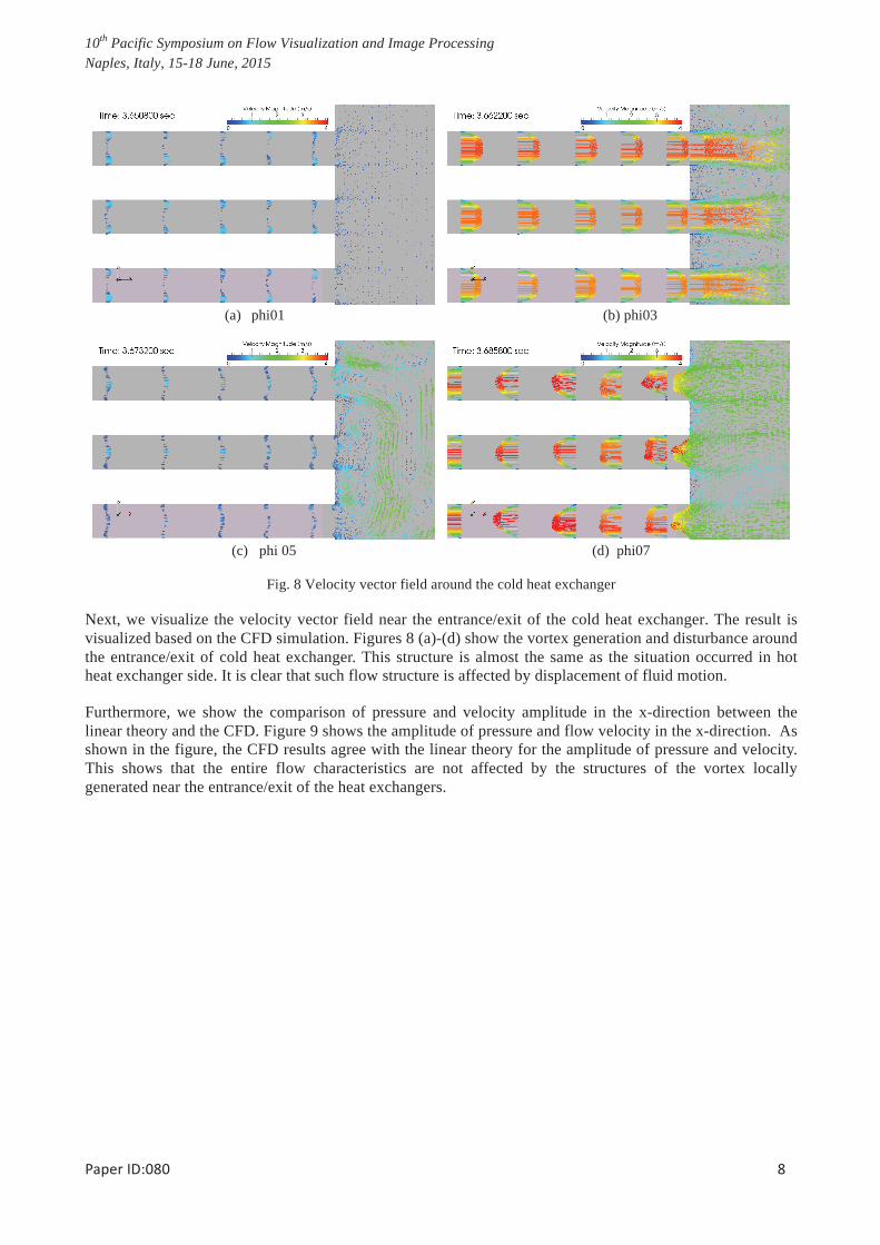
Fig. 8 Velocity vector field around the cold heat exchanger

Next, we visualize the velocity vector field near the entrance/exit of the cold heat exchanger. The result is visualized based on the CFD simulation. Figures 8 (a)-(d) show the vortex generation and disturbance around the entrance/exit of cold heat exchanger. This structure is almost the same as the situation occurred in hot heat exchanger side. It is clear that such flow structure is affected by displacement of fluid motion.

Furthermore, we show the comparison of pressure and velocity amplitude in the x-direction between the linear theory and the CFD. Figure 9 shows the amplitude of pressure and flow velocity in the x-direction. As shown in the figure, the CFD results agree with the linear theory for the amplitude of pressure and velocity. This shows that the entire flow characteristics are not affected by the structures of the vortex locally generated near the entrance/exit of the heat exchangers.


Fig. 14 Velocity and pressure amplitude distribution in the x direction of the tube

Fig. 15 Workflow distributions in the x-direction of the experiment

5 Summary

In order to investigate the phenomena occurred in the thermoacoustic device, we conducted the experiment using PIV, and also carried out the CFD simulation. From the results, we conclude as follows.

Using PIV, we could visualize the disturbance and vortex generation around the heat exchanger, which is occurred by the displacement of fluid motion. Furthermore, we could also reproduce those phenomena in the CFD.

The results of CFD agree with the experimental data for the velocity vector field around the engine, and also agree with the linear theory for the amplitude of pressure and velocity in the x direction. This

0

150

300

450

600

750

900

0 0.5 1 1.5 2 2.5 3 3.5 4 4.5 0

0.5

1

1.5

2

2.5

3

P (

Pa)

u (m

/s)

x(m)

p exp.(lft tube.)p exp.(rht tube.)

p ana.u exp.(lft tube.)

u exp.(rht tube.)u ana.

-0.015

-0.01

-0.005

0

0.005

0.01

0.015

0.02

0.025

0 0.5 1 1.5 2 2.5 3 3.5 4 4.5

Wor

kflo

w (

W)

x(m)

exp. (lft tube)exp. (rht tube)

ana. (Tw=448.15K)ana. (Tw=386.15K)


implies that the effect of local disturbance around the engine is not so large for the entire characteristics of fluid motion.

From the results of CFD, we could investigate the effect of the displacement of fluid motion on the heat transfer in the engine. As a result, we confirmed the relationship between the displacement and the efficiency of the engine qualitatively.

In order to obtain the high efficiency of the engine, we need to make clear the quantitative relationship between the displacement of fluid motion and the amount of heat transfer in the engine. This is remained as a future work.

Acknowledgement

This work was supported by the Japan Science and Technology Agency through the Advanced Low Carbon Technology Research and Development Program.

References

[1] Backhaus, S. N. and Swift, G. W., Nature 399, 335-338 (1999).

[2] Kirchhoff, G. R., Pogg. Ann. 134, 177-193 (1868).

[3] Rayleigh, J. W. S., The Theory of Sound, Vol. II, Dover, New York, 319-326 (1945).

Zwikker, C. and Kosten, C. W., Sound Absorbing Materials, Elsevier, Amsterdam, 25–52 (1949).

[5] Weston, D. E., Proc. Phys. Soc. London B.66, 695–709 (1953).

[6] Iberall, A. S., J. Res. Nat. Bur. Stand. 45, 85–108 (1950).

[7] Rott, N., Zeitschrift für angewandte Mathematik und Physik ZAMP 20(2), 230–243 (1969).

[8] Tijdeman, H., J.Sound Vib. 39, 1–33 (1975).

[9] Piccolo, A. and Pistone, G., Int. J. Heat Mass Tran, 49, 1631-1642 (2006).

[10] Jaworski, A. J., Mao, X. and Yu, Z., Experimental Thermal and Fluid Science 33, 459–502 (2009).

[11] Shi, L., Yu, Z. and Jaworski, A. J., International Journal of Thermal Sciences 49, 1688–1701 (2010).

[12] Shi, L., Yu, Z. and Jaworski, A. J., European Journal of Mechanics B/Fluids 30, 206–217 (2011).

[13] Jaworski , A. J. and Piccolo , A., Applied Thermal Engineering 42, 145–153 (2012).

[14] Fusco, A. M., Ward, W. C. and Swift, G. W., J. Acoust. Soc. Am. 91(4)-1, 2229–2235 (1992).

[15] Jameson, A. and Turkel, E., Mathematics of Computation, Vol.37, No.156, 385-397 (1981).

[16] Shima, E., and Kitamura, K., AIAA Journal (to be published); see also AIAA 2009-136 (2009).

[17] Wang, Z. J., Computers and Fluids, Vol.27, 529-549 (1998).

measurement and visualization of oscillatory flow in a

Documents