measurement investigation of gravity waves using ... · pdf file2894 g. stober et al.:...

Atmos. Meas. Tech., 6, 2893–2905, 2013www.atmos-meas-tech.net/6/2893/2013/doi:10.5194/amt-6-2893-2013© Author(s) 2013. CC Attribution 3.0 License.

Atmospheric Measurement

TechniquesO

pen Access

Investigation of gravity waves using horizontally resolved radialvelocity measurements

G. Stober1, S. Sommer1, M. Rapp2,3, and R. Latteck1

1Leibniz-Institute of Atmospheric Physics at the Rostock University, Schlossstr. 6, 18225 Kühlungsborn, Germany2Deutsches Zentrum für Luft- und Raumfahrt, Institut für Physik der Atmosphäre, Oberpfaffenhofen, Germany3Meteorologisches Institut München, Ludwig-Maximilian Universität München, Munich, Germany

Correspondence to:G. Stober ([email protected])

Received: 27 May 2013 – Published in Atmos. Meas. Tech. Discuss.: 25 June 2013Revised: 4 September 2013 – Accepted: 26 September 2013 – Published: 30 October 2013

Abstract. The Middle Atmosphere Alomar Radar System(MAARSY) on the island of Andøya in Northern Nor-way (69.3◦ N, 16.0◦ E) observes polar mesospheric summerechoes (PMSE). These echoes are used as tracers of atmo-spheric dynamics to investigate the horizontal wind variabil-ity at high temporal and spatial resolution. MAARSY has thecapability of pulse-to-pulse beam steering allowing for sys-tematic scanning experiments to study the horizontal struc-ture of the backscatterers as well as to measure the radial ve-locities for each beam direction. Here we present a methodto retrieve gravity wave parameters from these horizontallyresolved radial wind variations by applying velocity azimuthdisplay and volume velocity processing. Based on the ob-servations a detailed comparison of the two wind analysistechniques is carried out in order to determine the zonal andmeridional wind as well as to measure first-order inhomo-geneities. Further, we demonstrate the possibility to resolvethe horizontal wave properties, e.g., horizontal wavelength,phase velocity and propagation direction. The robustness ofthe estimated gravity wave parameters is tested by a simpleatmospheric model.

1 Introduction

The mesosphere/lower thermosphere region (MLT) is char-acterized by a high temporal and spatial variability due toplanetary and gravity waves. Gravity waves (GW) are animportant driver of the atmospheric dynamics. They carryenergy and momentum from their source regions and de-posit them far away from the point of origin, altering the

circulation pattern in the middle atmosphere (e.g.,Fritts andAlexander, 2003; Becker, 2012).

There are several in situ (e.g.,Eckermann and Vincent,1989; Theuerkauf et al., 2011) and ground-based observa-tion techniques like, e.g., meteor radars (e.g.,Hocking, 2005;Fritts et al., 2010b, a; Placke et al., 2011), MF radars (e.g.,Hoffmann et al., 2010, 2011; Placke et al., 2013), lidars(e.g.,Rauthe et al., 2006; Gerding et al., 2008), airglow im-agers (e.g.,Nakamura et al., 1999; Pautet and Moreels, 2002;Suzuki et al., 2004, 2010) or CCD images of noctilucentclouds (NLC) (e.g.,Pautet et al., 2011) as well as satellite-borne observations (e.g.,Preusse et al., 2000; Ern et al., 2004,2011) to quantify the properties of gravity waves and their ef-fect on the background flow. Here we investigate short-periodgravity waves using horizontally resolved radar observations.

MAARSY is dedicated to accessing the horizontal windvariability. The radar is capable to perform pulse-to-pulsebeam steering allowing to conduct systematic scanning ex-periments. During summer 2011 MAARSY was operatedemploying 97 different beam directions to observe the hor-izontal variability of polar mesospheric summer echoes(PMSE). Some initial results of the properties of gravitywaves using MAARSY multi-beam experiments have beenderived from the pure morphology of the observed echoesas discussed inRapp et al.(2011). In the current paper, thenext step to determining the wave properties is taken, that is,the PMSE backscatter (e.g.,Rapp and Lübken, 2004) is usedas a tracer to deduce the horizontal variability of mesosphericwinds by applying a velocity azimuth display analysis (VAD)(Browning and Wexler, 1968) and volume velocity process-ing (VVP) algorithm (Waldteufel and Corbin, 1979).

Published by Copernicus Publications on behalf of the European Geosciences Union.

2894 G. Stober et al.: Investigation of gravity waves

Here we demonstrate that scanning experiments are usefulto derive horizontally resolved radial velocity measurementsand how these images/snapshots of the horizontal wind vari-ability are analyzed with respect to gravity waves. Further,we evaluate our analysis method with a simple model similarto the approach presented inFritts et al.(2010a). This modelincludes a mean background flow and a superposition of twodominant GW. The meridional, zonal and vertical GW am-plitudes are coupled by the linear polarization relations forGW. The vertical wavelength is given by the dispersion equa-tion (e.g.,Fritts and Alexander, 2003; Suzuki et al., 2010) forshort-period GW.

The manuscript is structured as follows. Section 2 con-tains a short technical description of the radar and the experi-ment. Section 3 provides an overview over the general PMSEconditions during the observations, including a selected 3-Dcase of the PMSE structure. In Sect. 4 we present a short in-troduction of the VAD and VVP technique. The mean windsituation for the investigated period is described in Sect. 5,which includes a comparison of the VAD and VVP windmeasurements. Section 6 contains a method to create 2-D ra-dial velocity variation images and how such images can beanalysed regarding gravity waves using modelling results. InSect. 7 we describe our analysis procedure and demonstratethe ability to retrieve GW parameters based on four cases.The results are summarized and discussed in Sect. 8.

2 MAARSY multi-beam experiments

MAARSY employs an active-phased array antenna consist-ing of 433 linearly polarized Yagi antennas. Each of the an-tennas is connected to its own transceiver module, which isadjustable in power and phase. This design permits to steerthe beam on a pulse-to-pulse basis. A more detailed tech-nical description of the radar is presented inLatteck et al.(2010, 2012). Making use of this rapid beam steering ca-pability, MAARSY is able to conduct systematic scanningexperiments covering an area of about 80 km in diameter atmesospheric heights. The number of different beam direc-tions per experiment is mainly given by the required Nyquistfrequency to ensure reliable radial velocity measurements.With an increasing off-zenith angle the radial Doppler shiftincreases as well, due to the horizontal winds.

During summer 2011 MAARSY was operated in a multi-beam mode with 97 different beam directions. This wasachieved by a sequence of four experiments containing25 beams each. The vertical beam was included in each ex-periment, leading to 97 individual and unambiguous beamdirections. In Fig.1 a projection of all 97 beam directions at85 km altitude is shown. The black lines indicate the coastline of Northern Norway. The diameter of the red circles cor-responds to a beam width of 3.6◦. The beam positions foreach of the four experiments are shown in Fig.2.

Discu

ssionPaper

|Discu

ssionPaper

|Discu

ssionPaper

|Discu

ssionPaper

|

14oE 15oE 16oE 17oE 18oE

40’

69oN

20’

40’

70oN

Fig. 1. Beam position of MAARSY scanning experiment during summer 2011. The black contour linesindicate the Northern Norwegian coast line. The red circles represent the beam positions assuming a 3.6◦

beam width at 84 km.

26

Fig. 1. Beam position of MAARSY scanning experiment duringsummer 2011. The black contour lines indicate the Northern Nor-wegian coast line. The red circles represent the beam positions as-suming a 3.6◦ beam width at 84 km.

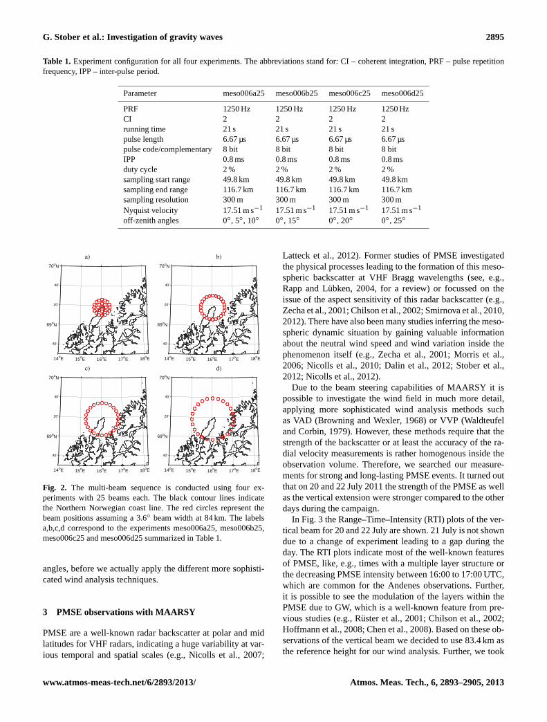
In Table1 the experiment parameters are summarized. Theorder of the experiments corresponds to the labels of the pan-els a–d in Fig.2. In particular, the experiments meso006b25,meso006c25 and meso006d25 were designed to be analyzedapplying a velocity azimuth display analysis, viz. the ra-dial velocity is measured for 24 different azimuth directions,whereas the zenith angle is kept constant for each of the sub-experiments. A critical point in performing such multi-beamexperiments is the Nyquist frequency. The PMSE observa-tions are carried out with a pulse repetition frequency (PRF)of 1250 Hz. This PRF avoids any issues with range aliasingeffects. On the other hand a higher PRF would be desirable toincrease the Nyquist frequency or the corresponding Nyquistvelocity, which is equivalent to the highest observable un-aliased due to the limited horizontal wind speed.

In particular, the radial velocities for off-zenith angleslarger than 10◦ could be aliased due to limited Nyquist veloc-ity. Therefore, each radial velocity measurement is checkedfor a likely aliasing and – if possible – is unwrapped. This isdone by computing an initial mean prevailing wind estimatejust using the beam directions from experiment meso006a25.The wind is computed by using a straight-forward DopplerBeam Swinging method (DBS). Based on the prevailingzonal and meridional wind it is possible to compute a ra-dial velocity for each beam direction, which is compared tothe measured one. By simply adding or subtracting multiplesof the Nyquist velocity we unwrap likely aliased radial veloc-ity measurements from the experiments with larger off-zenith

Atmos. Meas. Tech., 6, 2893–2905, 2013 www.atmos-meas-tech.net/6/2893/2013/

G. Stober et al.: Investigation of gravity waves 2895

Table 1. Experiment configuration for all four experiments. The abbreviations stand for: CI – coherent integration, PRF – pulse repetitionfrequency, IPP – inter-pulse period.

Parameter meso006a25 meso006b25 meso006c25 meso006d25

PRF 1250 Hz 1250 Hz 1250 Hz 1250 HzCI 2 2 2 2running time 21 s 21 s 21 s 21 spulse length 6.67 µs 6.67 µs 6.67 µs 6.67 µspulse code/complementary 8 bit 8 bit 8 bit 8 bitIPP 0.8 ms 0.8 ms 0.8 ms 0.8 msduty cycle 2 % 2 % 2 % 2 %sampling start range 49.8 km 49.8 km 49.8 km 49.8 kmsampling end range 116.7 km 116.7 km 116.7 km 116.7 kmsampling resolution 300 m 300 m 300 m 300 mNyquist velocity 17.51 m s−1 17.51 m s−1 17.51 m s−1 17.51 m s−1

off-zenith angles 0◦, 5◦, 10◦ 0◦, 15◦ 0◦, 20◦ 0◦, 25◦Discu

ssionPaper

|Discu

ssionPaper

|Discu

ssionPaper

|Discu

ssionPaper

|

a) b)


40’

69oN

20’

40’

70oN


40’

69oN

20’

40’

70oN

c) d)


40’

69oN

20’

40’

70oN


40’

69oN

20’

40’

70oN

27Fig. 2. The multi-beam sequence is conducted using four ex-periments with 25 beams each. The black contour lines indicatethe Northern Norwegian coast line. The red circles represent thebeam positions assuming a 3.6◦ beam width at 84 km. The labelsa,b,c,d correspond to the experiments meso006a25, meso006b25,meso006c25 and meso006d25 summarized in Table1.

angles, before we actually apply the different more sophisti-cated wind analysis techniques.

3 PMSE observations with MAARSY

PMSE are a well-known radar backscatter at polar and midlatitudes for VHF radars, indicating a huge variability at var-ious temporal and spatial scales (e.g.,Nicolls et al., 2007;

Latteck et al., 2012). Former studies of PMSE investigatedthe physical processes leading to the formation of this meso-spheric backscatter at VHF Bragg wavelengths (see, e.g.,Rapp and Lübken, 2004, for a review) or focussed on theissue of the aspect sensitivity of this radar backscatter (e.g.,Zecha et al., 2001; Chilson et al., 2002; Smirnova et al., 2010,2012). There have also been many studies inferring the meso-spheric dynamic situation by gaining valuable informationabout the neutral wind speed and wind variation inside thephenomenon itself (e.g.,Zecha et al., 2001; Morris et al.,2006; Nicolls et al., 2010; Dalin et al., 2012; Stober et al.,2012; Nicolls et al., 2012).

Due to the beam steering capabilities of MAARSY it ispossible to investigate the wind field in much more detail,applying more sophisticated wind analysis methods suchas VAD (Browning and Wexler, 1968) or VVP (Waldteufeland Corbin, 1979). However, these methods require that thestrength of the backscatter or at least the accuracy of the ra-dial velocity measurements is rather homogenous inside theobservation volume. Therefore, we searched our measure-ments for strong and long-lasting PMSE events. It turned outthat on 20 and 22 July 2011 the strength of the PMSE as wellas the vertical extension were stronger compared to the otherdays during the campaign.

In Fig. 3 the Range–Time–Intensity (RTI) plots of the ver-tical beam for 20 and 22 July are shown. 21 July is not showndue to a change of experiment leading to a gap during theday. The RTI plots indicate most of the well-known featuresof PMSE, like, e.g., times with a multiple layer structure orthe decreasing PMSE intensity between 16:00 to 17:00 UTC,which are common for the Andenes observations. Further,it is possible to see the modulation of the layers within thePMSE due to GW, which is a well-known feature from pre-vious studies (e.g.,Rüster et al., 2001; Chilson et al., 2002;Hoffmann et al., 2008; Chen et al., 2008). Based on these ob-servations of the vertical beam we decided to use 83.4 km asthe reference height for our wind analysis. Further, we took

www.atmos-meas-tech.net/6/2893/2013/ Atmos. Meas. Tech., 6, 2893–2905, 2013


Fig. 3. RTI plots of a PMSE as observed with MAARSY in the vertical beam direction with a vertical resolution of 300 m and temporalresolution of 5 min. The time is given in UTC.

into account the change of the vertical resolution due to thelarge off-zenith angle. An off-zenith angle of 25◦ in combi-nation with the MAARSY beam width of 3.6◦ leads to a ver-tical smearing of about 2.4 km at 83.4 km altitude, althoughthe range resolution is kept the same as for the vertical beam.

Figure4 shows the 3-D structure of the PMSE for threesuccessive measurements, after interpolating the observa-tions to a Cartesian grid using a cubic spline (Latteck et al.,2012). The image reveals the huge variability of the PMSEintensity on spatial scales of 10–15 km. It seems to be char-acteristic for the PMSE that the SNR can drop by more than10–20 dB within a distance of a few kilometers. As outlinedin Hoffmann et al.(2008), short-period GW are a likely causeof this high variability inside the PMSE layer. In particular,the up- and downward motion of the lower edge of the PMSEis likely explained by short-period GW.

4 VVP and VAD wind analysis to account for horizontalinhomogeneities in the wind field

Previous studies used different methods to infer the GWproperties from the wind field, such as wavelet spectra orhodograph analysis (e.g.,Hoffmann et al., 2008; Rapp et al.,2011; Placke et al., 2013). Here we want to make use ofmulti-beam experiments to reveal the horizontal wind vari-ability due to GW. Following the approach ofBrowning andWexler(1968) the wind field can be expressed as a Taylor se-ries for the horizontal wind components consisting of a meanprevailing zonal and meridional wind (labeled by index 0)and the first-order gradient terms:

u = u0 +∂u

∂x· x +

∂u

∂y· y

andv = v0 +∂v

∂x· x +

∂v

∂y· y. (1)

In Eq. (1)u denotes the zonal andv the meridional wind di-rection. Transforming the Cartesian coordinates into spheri-cal ones permits to express the radial wind velocityvrad independence of the azimuth (φ) and zenith (θ ) angle yields:

vrad(φ, θ) = u · cos(φ) sin(θ) + v · sin(φ) sin(θ)

+w cos(θ). (2)

The azimuth angleφ is referenced to the east and mea-sured counterclockwise andθ refers to the zenith distance.The mean vertical wind velocityw0 is assumed to be con-stant within the measurement volume. Using the approachof Browning and Wexler(1968) in Eq. (2) leads to an ex-pression of the radial velocity in dependence of the meanzonal, meridional and vertical wind and the first-order gradi-ent wind inhomogeneities.

The fact that the number of beam directions is larger thanthe number of unknowns (right-hand terms in Eq. 1) permitsto solve the set of equations using a least squares fit. Themajor difference between the VAD and VVP method is theway the fitting of the wind field is done. The basic idea ofthe VAD is to decompose Eq. (2) into its Fourier compo-nents (Browning and Wexler, 1968) and fitting for each of theFourier coefficients, whereas the VVP procedure directly fitsthe set of equations for all the unknown variables (Waldteufeland Corbin, 1979).

The MAARSY multi-beam experiments were analyzed us-ing both methods. The advantage of a VAD scan is thatone needs fewer measurements to gain information about thefirst-order inhomogeneities. In principle one needs no mea-surement from inside the scanning area. In the same time asone VVP scan with 97 beams, we can perform four VADscans. The disadvantage of the VAD technique is that it justuses a small portion of all the information gathered by the97-beam experiment. Another difficulty of a VAD analysisis that it does not allow to distinguish between the verticalwind velocity and the horizontal divergence inside the scan-ning volume just using one scan. Following the nomenclatureof Browning and Wexler(1968) the first Fourier coefficienta0 is given by

a0 = −r · sin(θ) · divh + 2w0 · cos(θ), (3)

wherer denotes the radius of the VAD scanning circle de-pending on the altitude or range and divh is the horizontal di-vergence. This issue is partly solved by an extended velocityazimuth display (EVAD) (Larsen et al., 1991; Matejka andSrivastava, 1991). Such an analysis combines several VADscans with different off-zenith angles to distinguish betweencontributions of the vertical wind velocity and the horizontaldivergence. For each of the off-zenith angles one measures


G. Stober et al.: Investigation of gravity waves 2897Discu

ssionPaper

|Discu

ssionPaper

|Discu

ssionPaper

|Discu

ssionPaper

|

Fig. 4. RTI plot of the 3-D structure of the PMSE for three successive scans from 20 July 2011. The SNRfor each beam direction was gridded using a cubic spline. The vertical distance between the horizontalslices is 1 km. The horizontal slices show a significant beam to beam as well as the temporal variability.

30

Fig. 4.RTI plots of the 3-D structure of the PMSE for three successive scans from 20 July 2011. The SNR for each beam direction was griddedusing a cubic spline. The vertical distance between the horizontal slices is 1 km. The horizontal slices show a significant beam-to-beam aswell as the temporal variability.

the coefficienta0, which, hence, permits to solve Eq. (3) withrespect to the horizontal divergence and the vertical velocity.

By applying a VVP fit, this problem is completely over-come and one gets an unambiguous result for the vertical ve-locity and the horizontal divergence within the observationvolume. In addition the VVP is more robust so as to deter-mine a prevailing mean wind, because the method can bet-ter deal with gaps/inhomogeneities of the PMSE backscat-ter. The VVP technique permits to determine a reliable windvelocity based on 50 % of the available different beam di-rections, whereas the VAD method tends to be more biasedby gaps along the scanning circle caused by the horizontalvariability of the PMSE backscatter. A VAD experiment wasonly analyzed when we had radial wind measurements from21 different azimuth directions out of the 24 oblique beamsalong one VAD circle.

5 VVP and VAD/EVAD wind comparison

The quasi-simultaneous multi-beam experiment is an idealpossibility to compare both techniques to understand theadvantages and disadvantages of both analysis procedures.Before we are going to compare both techniques we willhave a look at the background wind situation. In Fig.5 thedetermined zonal and meridional wind velocity within thescanning volume is shown. Both days indicate a dominat-ing semi-diurnal tidal structure in both components and amuch weaker diurnal tide. The zonal wind component showsa mean westerly flow at the altitude of the PMSE, whereasthe meridional wind component indicates a mean southwarddirection. Concerning the mean winds and the tidal structureboth days represent a typical polar summer situation. Notethat the vertical structure is mainly dominated by the off-zenith beams (zenith angle> 15◦), which leads to a vertical

smearing. The layered structure that can be found in the RTIplots (Fig.3) of the vertical beam disappears in the analyzedzonal and meridional wind fields due to this vertical smearingeffect.

The basic idea of the approach fromBrowning and Wexler(1968) was to use a Taylor series of the wind field to ac-count for first-order inhomogeneities in the wind field. TheMAARSY multi-beam observations are suitable to deter-mine these first-order distortions. In particular, the relationof the horizontal divergence and the vertical velocity shouldprovide some information about the GW activity. In Fig.6the computed vertical wind velocity and the horizontal di-vergence for both days are visualized. The vertical velocityshows values of±5 m s−1, which still seems to be slightlytoo large as a mean vertical velocity considering the observa-tion volume used here. The highest vertical velocities occurat edges of the PMSE layer and are likely related to rela-tively large deviations from the nominal off-zenith angle. Onthe other hand a visual inspection of the color bar demon-strates that the vertical velocity is most of the time close to0 m s−1, which in so far should be a good estimate for sucha huge volume. However, similar vertical velocities were ob-served byHoppe and Fritts(1995) using the EISCAT. On theother hand there are EISCAT measurements indicating evenhigher Doppler shifts of about±10 m s−1 (e.g.,Fritts et al.,1990; Strelnikova and Rapp, 2011, 2013).

Although it is not possible to identify single gravity waves,these two parameters visualize the high variability of thehorizontal wind field and the importance of consideringsuch inhomogeneities, in particular if one uses measurementsthat have a spatial separation of several kilometers. Thefirst-order distortions permit to estimate how the wind fieldchanges with increasing distance from the radar site. A hori-zontal gradient in the wind field in the order of 0.5× 10−3 1/scan lead to a 20 m s−1 change of the total wind velocity at a



Fig. 5.Observed zonal and meridional wind from MAARSY measurements using PMSE as tracer for 20 and 22 July 2011. The time is givenin UTC.

Fig. 6.Observed vertical and horizontal divergence wind from MAARSY measurements using PMSE as tracer for 20 and 22 July 2011. Thetime is given in UTC.

horizontal distance of 40 km. Hence, it can be of importanceto consider these horizontal differences, in particular if themeasurement volumes are not completely coincident. Thisshould be considered if one aims to compare different windobservation techniques that employ different beam point-ing directions or are spatially separated (e.g., lidar, meteorradars, satellite).

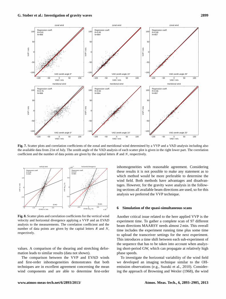
To get a first impression of how well both methods com-pare with each other, the observations were analyzed apply-ing the VVP technique using all available beam directionsand VAD scans for three different off-zenith angles. To avoidany difficulties with edge effects, only the observations froman altitude of 83.4 km were considered. The scatter plots ofVAD vs. VVP are shown in Fig.7. The correlation coeffi-cient and the number of data points are given by the capitallettersR andN , respectively. The red line indicates the slope1 regression and one black line is given by a linear fit to thescatter plot. The second black line is computed after swap-ping the x and y axes.

The comparison also includes some measurements from21 July 2011. Figure7 clearly visualizes that the correlationbetween both methods increases with increasing off-zenithangle. The best agreement is achieved between the VVP andVAD analysis for the 25◦ off-zenith angle. However, there is

still a reasonable agreement for the 5◦ off-zenith VAD scanand the VVP technique. This comparison provides two es-sential results: the VVP and the VAD analysis result in sim-ilar horizontal wind speeds as long as the volumes are thesame, viz. the VVP horizontal wind components are dom-inated by the largest off-zenith angle using the MAARSYbeam positions. The second point is that this comparison di-rectly provides a first idea of the horizontal variability of thewind field. The increased scattering of the 5◦ off-zenith VADscan vs. the VVP is likely caused by GW with horizontalwavelengths much shorter than the VVP scanning diame-ter. In the absence of such small-scale distortions the scatterplots should look almost identical, like for the 25◦ off-zenithangles.

Further, it is not very difficult to combine several VADscans to an EVAD analysis to resolve the ambiguity betweenhorizontal divergence and vertical velocity. In Fig.8 the scat-ter plots of the vertical wind velocity and horizontal diver-gence for EVAD vs. VVP are shown. The correlation coeffi-cients still indicate a generally reasonable agreement for bothparameters. The major difference is that the VVP tends tosystematic higher values for the vertical wind velocity andhorizontal divergence. Based on the available data it is notpossible to judge which method provides the more reliable


G. Stober et al.: Investigation of gravity waves 2899Discu

ssionPaper

|Discu

ssionPaper

|Discu

ssionPaper

|Discu

ssionPaper

|

−100 −50 0 50 100

−100

−50

0

50

100

VAD / m/s

VV

P /

m/s

zonal wind

Regression coeff.R=0.81 N=866

VAD zenith angle 5°

−100 −50 0 50 100

−100

−50

0

50

100

VAD / m/s

VV

P /

m/s

zonal wind



−100 −50 0 50 100

−100

−50

0

50

100

VAD / m/s

VV

P /

m/s

zonal wind



−100 −50 0 50 100

−100

−50

0

50

100

VAD / m/s

VV

P /

m/s

meridional wind



−100 −50 0 50 100

−100

−50

0

50

100

VAD / m/s

VV

P /

m/s

meridional wind



−100 −50 0 50 100

−100

−50

0

50

100

VAD / m/s

VV

P /

m/s

meridional wind



Fig. 7. Scatter plots and correlation coefficients of the zonal and meridional wind determined by a VVPor VAD analysis including also the available data from 21st of July. The zenith angle of the VADanalysis of each scatter plot is given in the right lower part. The correlation coefficient and the numberof data points are given by the capital letters R and N respectively.

33

Fig. 7. Scatter plots and correlation coefficients of the zonal and meridional wind determined by a VVP and a VAD analysis including alsothe available data from 21st of July. The zenith angle of the VAD analysis of each scatter plot is given in the right lower part. The correlationcoefficient and the number of data points are given by the capital lettersR andN , respectively.

Discu

ssionPaper

|Discu

ssionPaper

|Discu

ssionPaper

|Discu

ssionPaper

|

−5 −2.5 0 2.5 5−5

−2.5

0

2.5

5

EVAD w / m/s

VV

P w

/ m

/s

vertical wind


EVAD

−1 −0.5 0 0.5 1

x 10−3

−1

−0.5

0

0.5

1x 10

−3

EVAD divh/ 1/s

VV

P d

ivh/ 1

/s

horizontal divergence


EVAD

Fig. 8. Scatter plots and correlation coefficients for the vertical wind velocity and horizontal divergenceapplying a VVP and a EVAD analysis to the measurements. The correlation coefficient and the numberof data points are given by the capital letters R and N respectively.

34

Fig. 8.Scatter plots and correlation coefficients for the vertical windvelocity and horizontal divergence applying a VVP and an EVADanalysis to the measurements. The correlation coefficient and thenumber of data points are given by the capital lettersR and N ,respectively.

values. A comparison of the shearing and stretching defor-mation leads to similar results (data not shown).

The comparison between the VVP and EVAD windsand first-order inhomogeneities demonstrates that bothtechniques are in excellent agreement concerning the meanwind components and are able to determine first-order

inhomogeneities with reasonable agreement. Consideringthese results it is not possible to make any statement as towhich method would be more preferable to determine thewind field. Both methods have advantages and disadvan-tages. However, for the gravity wave analysis in the follow-ing sections all available beam directions are used, so for thisanalysis we preferred the VVP technique.

6 Simulation of the quasi-simultaneous scans

Another critical issue related to the here applied VVP is theexperiment time. To gather a complete scan of 97 differentbeam directions MAARSY needs almost 2 min. This overalltime includes the experiment running time plus some timeto upload the transceiver settings for the next experiment.This introduces a time shift between each sub-experiment ofthe sequence that has to be taken into account when analyz-ing short-period GW, which can propagate at relatively highphase speeds.

To investigate the horizontal variability of the wind fieldwe developed an imaging technique similar to the OH-emission observations (e.g.,Suzuki et al., 2010). Consider-ing the approach ofBrowning and Wexler(1968), the wind



field is decomposed into mean winds and the first-order gra-dient wind terms from Eq. (1), which are related to large-scale GW. “Large” refers here to the horizontal extension ofthe observation volume. These waves have horizontal wave-lengths much larger than the scanning diameter and periodsof several hours. Applying a VVP analysis permits to deter-mine the mean prevailing wind and these first-order inho-mogeneities. Hence, we can rewrite Eq. (2) and express theradial wind velocity for each azimuth and off-zenith angleby a mean zonal (u0), meridional (v0) and vertical (w0) windvelocity and the large-scale GW denoted byu′, v′ andw′:

vradVVP(φ, θ) = u0 · cos(φ)sin(θ) + v0 · sin(φ) sin(θ)

+w0 · cos(θ) + u′· cos(φ) sin(θ)

+v′· sin(φ) sin(θ) + w′

· cos(θ). (4)

The variablesu′, v′ andw′ refer to the gradient wind termsand their absolute values depend on the position inside themeasurement volume(u′, v′, w′)(φ, θ). On the other handMAARSY measures the radial wind velocity for each beamdirection, which contains contributions of the mean prevail-ing wind and a superposition of large-scale and small-scalewaves given byu′′, v′′ andw′′:

vradmeas(φ, θ) = u0 · cos(φ) sin(θ) + v0 · sin(φ) sin(θ)

+w0 · cos(θ) + u′· cos(φ) sin(θ)

+v′· sin(φ) sin(θ) + w′

· cos(θ)

+u′′· cos(φ) sin(θ) + v′′

· sin(φ) sin(θ)

+w′′· cos(θ). (5)

In Eq. (4) the parameter vradmeas represents the actuallymeasured radial velocity, which contains contributions of allwaves and wind field distortions. By subtracting Eq. (3) fromEq. (4) for each beam direction we obtain the radial velocityvariation inside the observation volume. In order to gener-ate an image of these radial wind variations, all 97 differentbeam directions are interpolated to a grid with a horizontalresolution of 250 m using a cubic spline, which results in aradial velocity variation image similar to the horizontally re-solved RTI images shown in Fig.4.

In order to test our decomposition of the wind field, weintroduce a simple atmospheric model similar toFritts et al.(2010a). The model assumes a mean background wind fieldincluding also the first-order wind gradient terms (e.g., hor-izontal divergence, stretching and shearing deformation) onwhich we superimpose monochromatic gravity waves withdifferent phase velocities, wind amplitudes, wavelengths andperiods. Further, we assume that the GW behave accordingto linear theory. The zonal, meridional and vertical wind dis-tortions (amplitudes) are linked by the polarization relationsof the GW (e.g.,Fritts and Alexander, 2003).

The simulated GW properties were selected to be repre-sentative of the gravity waves that one could expect at An-denes.Nielsen et al.(2006) analyzed short-period gravitywaves over Northern Norway using OH, Na and O2 emission

as well as meteor radar wind measurements from Andøyaand Esrange. The observed GW showed horizontal wave-lengths between 10–42 km and phase speeds of 29–72 m s−1.The intrinsic periods of the GW were determined to be in therange of 8–24 min.Pautet et al.(2011) investigated GW byusing NLC as a tracer of the dynamics. These observationswere carried out from Stockholm (59.4◦ N). Although thereis no absolute spatial coincidence between the observationvolumes, these GW observations from NLC provide at leastan idea of the GW properties that one could expect to mea-sure at Andenes (69.3◦ N) during the summer months.Pautetet al.(2011) found a variation of the phase velocities between10–60 m s−1 for most of the observed GWs and horizontalwavelengths in the range of 10–40 km.

In addition we considered that there is a small time shiftbetween each experiment and investigated the effect on theradial velocity variation image and whether the general GWproperties are preserved by the quasi-simultaneous multi-beam experiments. Therefore we conducted two simulationsassuming 25 and 125 s observation time between each ex-periment, which means that a complete scan consisting of97 beam positions takes 100 or 500 s, respectively. The ac-tual measurement time for each experiment was 20.48 s plusa few seconds for updating of all the transceiver modulesfor the next experiment (uploading new phases for the newbeam positions of the next experiment). Thus the 25 s case isa good approximation of the multi-beam observations con-ducted with MAARSY, which means it takes approximately100 s to measure one complete radial velocity variation im-age consisting of all 97 beam directions.

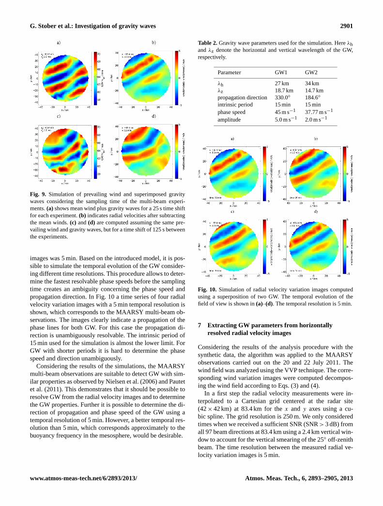
To test if there is a critical effect of a sampling delaybetween the quasi-simultaneous experiments we assume amean prevailing wind and the first-order inhomogeneities tobe in a similar range to our observations. To ensure a goodvisibility of the GW the first-order wind gradient terms areremoved from the images using the suggested decomposi-tion of the wind field. The gravity wave properties are givenin Table2. In Fig. 9 the horizontal wind variability for thetwo test cases is shown. Figure9a and c visualize the hor-izontal structure of the zonal wind and superimposed GW1and GW2. Figure9b and d represent radial velocity variationimages based on the above outlined procedure. As indicatedby Fig. 9a and b, a time delay of 25 s is not critical and theGW properties remain preserved in the radial velocity vari-ation image. Assuming a 125 s time shift between each suc-cessive experiment leads to a deformation of the GW phaselines due to the then too slow sampling of the image. TheGW structure appears to be bent and the wave structure isno longer preserved. For this case the phase velocity of theGW1 of 45 m s−1 is too fast to still be resolved using an ob-servation configuration of four sub-experiments with a 125 smeasurement time each.

The propagation of two superimposed GW within the fieldof view was also investigated using the same GW proper-ties as above (Table2). The temporal resolution between the



Fig. 9. Simulation of prevailing wind and superimposed gravitywaves considering the sampling time of the multi-beam experi-ments.(a) shows mean wind plus gravity waves for a 25 s time shiftfor each experiment.(b) indicates radial velocities after subtractingthe mean winds.(c) and(d) are computed assuming the same pre-vailing wind and gravity waves, but for a time shift of 125 s betweenthe experiments.

images was 5 min. Based on the introduced model, it is pos-sible to simulate the temporal evolution of the GW consider-ing different time resolutions. This procedure allows to deter-mine the fastest resolvable phase speeds before the samplingtime creates an ambiguity concerning the phase speed andpropagation direction. In Fig.10 a time series of four radialvelocity variation images with a 5 min temporal resolution isshown, which corresponds to the MAARSY multi-beam ob-servations. The images clearly indicate a propagation of thephase lines for both GW. For this case the propagation di-rection is unambiguously resolvable. The intrinsic period of15 min used for the simulation is almost the lower limit. ForGW with shorter periods it is hard to determine the phasespeed and direction unambiguously.

Considering the results of the simulations, the MAARSYmulti-beam observations are suitable to detect GW with sim-ilar properties as observed byNielsen et al.(2006) andPautetet al.(2011). This demonstrates that it should be possible toresolve GW from the radial velocity images and to determinethe GW properties. Further it is possible to determine the di-rection of propagation and phase speed of the GW using atemporal resolution of 5 min. However, a better temporal res-olution than 5 min, which corresponds approximately to thebuoyancy frequency in the mesosphere, would be desirable.

Table 2.Gravity wave parameters used for the simulation. Hereλhandλz denote the horizontal and vertical wavelength of the GW,respectively.

Parameter GW1 GW2

λh 27 km 34 kmλz 18.7 km 14.7 kmpropagation direction 330.0◦ 184.6◦

intrinsic period 15 min 15 minphase speed 45 m s−1 37.77 m s−1

amplitude 5.0 m s−1 2.0 m s−1

Fig. 10. Simulation of radial velocity variation images computedusing a superposition of two GW. The temporal evolution of thefield of view is shown in(a)–(d). The temporal resolution is 5 min.

7 Extracting GW parameters from horizontallyresolved radial velocity images

Considering the results of the analysis procedure with thesynthetic data, the algorithm was applied to the MAARSYobservations carried out on the 20 and 22 July 2011. Thewind field was analyzed using the VVP technique. The corre-sponding wind variation images were computed decompos-ing the wind field according to Eqs. (3) and (4).

In a first step the radial velocity measurements were in-terpolated to a Cartesian grid centered at the radar site(42× 42 km) at 83.4 km for thex and y axes using a cu-bic spline. The grid resolution is 250 m. We only consideredtimes when we received a sufficient SNR (SNR> 3 dB) fromall 97 beam directions at 83.4 km using a 2.4 km vertical win-dow to account for the vertical smearing of the 25◦ off-zenithbeam. The time resolution between the measured radial ve-locity variation images is 5 min.



Table 3.Determined gravity wave parameters estimated from the radial wind variation images. Herec denotes the intrinsic phase speed,λhthe horizontal wavelength and “az” the azimuth angle of the propagation direction.

date and time λh c az duration

20 July 2011, 05:10 UTC 28± 3 km 77± 10 m s−1 330.0◦ 30 min20 July 2011, 06:20 UTC 24± 5 km 43± 7 m s−1 229.6◦ 20 min20 July 2011, 22:30 UTC 47± 6 km 15± 2 m s−1 292.8◦/112.8◦ 20 min22 July 2011, 11:10 UTC 23± 3 km 12± 3 m s−1 332.4◦/152.4◦ 15 min

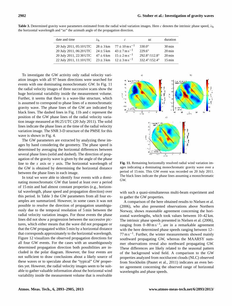
To investigate the GW activity only radial velocity vari-ation images with all 97 beam directions were searched forevents with one dominating monochromatic GW. In Fig.11the radial velocity images of three successive scans show thehuge horizontal variability inside the measurement volume.Further, it seems that there is a wave-like structure, whichis assumed to correspond to phase lines of a monochromaticgravity wave. The phase lines of the GW are indicated byblack lines. The dashed lines in Fig.11b and c represent theposition of the GW phase lines of the radial velocity varia-tion image measured at 06:25 UTC (20 July 2011). The solidlines indicate the phase lines at the time of the radial velocityvariation image. The SNR 3-D structure of the PMSE for thiswave is shown in Fig.4.

The GW parameters are extracted by analyzing these im-ages by hand considering the geometry. The phase speed isdetermined by averaging the horizontal differences betweenseveral phase lines (solid and dashed). The direction of prop-agation of the gravity wave is given by the angle of the phaseline to thex axis or y axis. The horizontal wavelength ofthe GW is obtained by determining the horizontal distancebetween the phase lines in each image.

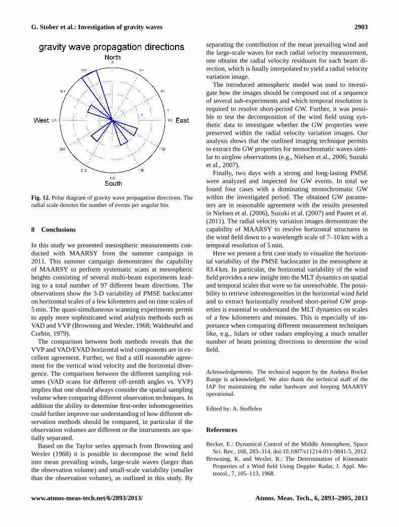
In total we were able to identify four events with a domi-nating monochromatic GW that lasted at least over a periodof 15 min and had almost constant properties (e.g., horizon-tal wavelength, phase speed and propagation direction) overthis period. In Table3 the GW parameters from all four ex-amples are summarized. However, in some cases it was notpossible to resolve the direction of propagation unambigu-ously due to the temporal resolution of 5 min between theradial velocity variation images. For those events the phaselines did not show a progression between the successive pic-tures, which either means that the wave did not propagate orthat the GW propagated within 5 min by a horizontal distancethat corresponds approximately to the horizontal wavelength.Figure12 visualizes the observed propagation directions forall four GW events. For the cases with an unambiguouslydetermined propagation direction both possibilities are in-cluded in the polar diagram. However, the four events arenot sufficient to draw conclusions about a likely source ofthese waves or to speculate about the “typical” GW proper-ties yet. However, the radial velocity images seem to be suit-able to gather valuable information about the horizontal windvariability inside the measurement volume that is resolvable

Discu

ssionPaper

|Discu

ssionPaper

|Discu

ssionPaper

|Discu

ssionPaper

|

a) b)

c)

Fig. 11. Remaining horizontally resolved radial wind variation images indicating a dominatingmonochromatic gravity wave over a period of 15 min. This GW event was recorded on 20 July 2011.The black lines indicate the phase lines assuming a monochromatic GW.

37

Fig. 11.Remaining horizontally resolved radial wind variation im-ages indicating a dominating monochromatic gravity wave over aperiod of 15 min. This GW event was recorded on 20 July 2011.The black lines indicate the phase lines assuming a monochromaticGW.

with such a quasi-simultaneous multi-beam experiment andto gather the GW properties.

A comparison of the here obtained results toNielsen et al.(2006), who also presented observations above NorthernNorway, shows reasonable agreement concerning the hori-zontal wavelengths, which took values between 10–42 km.The intrinsic phase speeds presented inNielsen et al.(2006),ranging from 0–80 m s−1, are in a remarkable agreementwith the here determined phase speeds ranging between 12–77 m s−1. Further, the winter measurements showed mainlysouthward propagating GW, whereas the MAARSY sum-mer observations reveal also northward propagating GW.These differences are likely related to the seasonal patternof the background wind field. A comparison to the GWproperties analyzed from noctilucent clouds (NLC) observedfrom Stockholm (Pautet et al., 2011) indicates an even bet-ter agreement concerning the observed range of horizontalwavelengths and phase speeds.



Discu

ssionPaper

|Discu

ssionPaper

|Discu

ssionPaper

|Discu

ssionPaper

|

Fig. 12. Polar diagram of gravity wave propagation directions. The radial scale denote the number ofevents per angular bin.

38

Fig. 12.Polar diagram of gravity wave propagation directions. Theradial scale denotes the number of events per angular bin.

8 Conclusions

In this study we presented mesospheric measurements con-ducted with MAARSY from the summer campaign in2011. This summer campaign demonstrates the capabilityof MAARSY to perform systematic scans at mesosphericheights consisting of several multi-beam experiments lead-ing to a total number of 97 different beam directions. Theobservations show the 3-D variability of PMSE backscatteron horizontal scales of a few kilometers and on time scales of5 min. The quasi-simultaneous scanning experiments permitto apply more sophisticated wind analysis methods such asVAD and VVP (Browning and Wexler, 1968; Waldteufel andCorbin, 1979).

The comparison between both methods reveals that theVVP and VAD/EVAD horizontal wind components are in ex-cellent agreement. Further, we find a still reasonable agree-ment for the vertical wind velocity and the horizontal diver-gence. The comparison between the different sampling vol-umes (VAD scans for different off-zenith angles vs. VVP)implies that one should always consider the spatial samplingvolume when comparing different observation techniques. Inaddition the ability to determine first-order inhomogeneitiescould further improve our understanding of how different ob-servation methods should be compared, in particular if theobservation volumes are different or the instruments are spa-tially separated.

Based on the Taylor series approach fromBrowning andWexler (1968) it is possible to decompose the wind fieldinto mean prevailing winds, large-scale waves (larger thanthe observation volume) and small-scale variability (smallerthan the observation volume), as outlined in this study. By

separating the contribution of the mean prevailing wind andthe large-scale waves for each radial velocity measurement,one obtains the radial velocity residuum for each beam di-rection, which is finally interpolated to yield a radial velocityvariation image.

The introduced atmospheric model was used to investi-gate how the images should be composed out of a sequenceof several sub-experiments and which temporal resolution isrequired to resolve short-period GW. Further, it was possi-ble to test the decomposition of the wind field using syn-thetic data to investigate whether the GW properties werepreserved within the radial velocity variation images. Ouranalysis shows that the outlined imaging technique permitsto extract the GW properties for monochromatic waves simi-lar to airglow observations (e.g.,Nielsen et al., 2006; Suzukiet al., 2007).

Finally, two days with a strong and long-lasting PMSEwere analyzed and inspected for GW events. In total wefound four cases with a dominating monochromatic GWwithin the investigated period. The obtained GW parame-ters are in reasonable agreement with the results presentedin Nielsen et al.(2006), Suzuki et al.(2007) andPautet et al.(2011). The radial velocity variation images demonstrate thecapability of MAARSY to resolve horizontal structures inthe wind field down to a wavelength scale of 7–10 km with atemporal resolution of 5 min.

Here we present a first case study to visualize the horizon-tal variability of the PMSE backscatter in the mesosphere at83.4 km. In particular, the horizontal variability of the windfield provides a new insight into the MLT dynamics on spatialand temporal scales that were so far unresolvable. The possi-bility to retrieve inhomogeneities in the horizontal wind fieldand to extract horizontally resolved short-period GW prop-erties is essential to understand the MLT dynamics on scalesof a few kilometers and minutes. This is especially of im-portance when comparing different measurement techniqueslike, e.g., lidars or other radars employing a much smallernumber of beam pointing directions to determine the windfield.

Acknowledgements.The technical support by the Andøya RocketRange is acknowledged. We also thank the technical staff of theIAP for maintaining the radar hardware and keeping MAARSYoperational.

Edited by: A. Stoffelen

References

Becker, E.: Dynamical Control of the Middle Atmosphere, SpaceSci. Rev., 168, 283–314, doi:10.1007/s11214-011-9841-5, 2012.

Browning, K. and Wexler, R.: The Determination of KinematicProperties of a Wind field Using Doppler Radar, J. Appl. Me-teorol., 7, 105–113, 1968.


http://dx.doi.org/10.1007/s11214-011-9841-5


Chen, J.-S., Hoffmann, P., Zecha, M., and Hsieh, C.-H.: Coherentradar imaging of mesosphere summer echoes: Influence of radarbeam pattern and tilted structures on atmospheric echo center,Radio Sci., 43, RS1002, doi:10.1029/2006RS003593, 2008.

Chilson, P. B., Yu, T.-Y., Palmer, R. D., and Kirkwood, S.: Aspectsensitivity measurements of polar mesosphere summer echoesusing coherent radar imaging, Ann. Geophys., 20, 213–223,doi:10.5194/angeo-20-213-2002, 2002.

Dalin, P., Kirkwood, S., Hervig, M., Mihalikova, M., Mikhaylova,D., Wolf, I., and Osepian, A.: Wave influence on polar meso-sphere summer echoes above Wasa: experimental and modelstudies, Ann. Geophys., 30, 1143–1157, doi:10.5194/angeo-30-1143-2012, 2012.

Eckermann, S. D. and Vincent, R. A.: Falling sphere observa-tions of anisotropic gravity wave motions in the upper strato-sphere over Australia, Pure Appl. Geophys., 130, 509–532,doi:10.1007/BF00874472, 1989.

Ern, M., Preusse, P., Alexander, M. J., and Warner, C. D.:Absolute values of gravity wave momentum flux derivedfrom satellite data, J. Geophys. Res.-Atmos., 109, D20103,doi:10.1029/2004JD004752, 2004.

Ern, M., Preusse, P., Gille, J. C., Hepplewhite, C. L., Mlynczak,M. G., Russell, J. M., and Riese, M.: Implications for atmo-spheric dynamics derived from global observations of gravitywave momentum flux in stratosphere and mesosphere, J. Geo-phys. Res.-Atmos., 116, D19107, doi:10.1029/2011JD015821,2011.

Fritts, D. and Alexander, M. J.: Gravity wave dynamics andeffects in the middle atmosphere, Rev. Geophys., 41, 1–64,doi:10.1029/2001RG000106, 2003.

Fritts, D., Hoppe, U.-P., and Inhester, B.: A study of the ver-tical motion field near the high-latitude summer mesopauseduring MAC/SINE, J. Atmos. Terr. Phys., 52, 927–938,doi:10.1016/0021-9169(90)90025-I, 1990.

Fritts, D. C., Janches, D., and Hocking, W. K.: Southern Ar-gentina Agile Meteor Radar: Initial assessment of gravity wavemomentum fluxes, J. Geophys. Res.-Atmos., 115, D19123,doi:10.1029/2010JD013891, 2010a.

Fritts, D. C., Janches, D., Iimura, H., Hocking, W. K., Mitchell,N. J., Stockwell, R. G., Fuller, B., Vandepeer, B., Hormaechea,J., Brunini, C., and Levato, H.: Southern Argentina Agile Me-teor Radar: System design and initial measurements of large-scale winds and tides, J. Geophys. Res.-Atmos., 115, D18112,doi:10.1029/2010JD013850, 2010b.

Gerding, M., Höffner, J., Lautenbach, J., Rauthe, M., and Lübken,F.-J.: Seasonal variation of nocturnal temperatures between 1 and105 km altitude at 54◦ N observed by lidar, Atmos. Chem. Phys.,8, 7465–7482, doi:10.5194/acp-8-7465-2008, 2008.

Hocking, W. K.: A new approach to momentum flux determinationsusing SKiYMET meteor radars, Ann. Geophys., 23, 2433–2439,doi:10.5194/angeo-23-2433-2005, 2005.

Hoffmann, P., Rapp, M., Fiedler, J., and Latteck, R.: Influenceof tides and gravity waves on layering processes in the po-lar summer mesopause region, Ann. Geophys., 26, 4013–4022,doi:10.5194/angeo-26-4013-2008, 2008.

Hoffmann, P., Becker, E., Singer, W., and Placke, M.: Sea-sonal variation of mesospheric waves at northern middleand high latitudes, J. Atmos. Sol.-Terr. Phy., 72, 1068–1079,doi:10.1016/j.jastp.2010.07.002, 2010.

Hoffmann, P., Rapp, M., Singer, W., and Keuer, D.: Trendsof mesospheric gravity waves at northern middle lati-tudes during summer, J. Geophys. Res., 116, D00P08,doi:10.1029/2011JD015717, 2011.

Hoppe, U.-P. and Fritts, D. C.: High-resolution measurements ofvertical velocity with the European incoherent scatter VHF radar:1. Motion field characteristics and measurement biases, J. Geo-phys. Res.-Atmos., 100, 16813–16825, doi:10.1029/95JD01466,1995.

Larsen, M., Fukao, S., Aruga, O., Yamanaka, M., Tsuda, T., andKato, S.: A Comparison of VHF Radar Vertical-Velocity Mea-surements by a Direct Vertical-Beam Method and by a VADTechnique, J. Atmos. Ocean. Tech., 8, 766–776, 1991.

Latteck, R., Singer, W., Rapp, M., and Renkwitz, T.: MAARSY thenew MST radar on Andøya/Norway, Adv. Radio Sci., 8, 219–224, doi:10.5194/ars-8-219-2010, 2010.

Latteck, R., Singer, W., Rapp, M., Vandepeer, B., Renkwitz, T.,Zecha, M., and Stober, G.: MAARSY: The new MST radaron Andøya-System description and first results, Radio Sci., 47,RS1006, doi:10.1029/2011RS004775, 2012.

Matejka, T. and Srivastava, R. C.: An Improved Version of theExtended Velocity-Azimuth Display Analysis of Single-DopplerRadar Data, J. Atmos. Ocean. Tech., 8, 453–466, 1991.

Morris, R., Murphy, D., Vincent, R., Holdsworth, D., Klekociuk,A., and Reid, I.: Characteristics of the wind, temperature andPMSE field above Davis, Antarctica, J. Atmos. Sol.-Terr. Phys.,68, 418–435, doi:10.1016/j.jastp.2005.04.011, 2006.

Nakamura, T., Higashikawa, A., Tsuda, T., and Matsushita, Y.: Sea-sonal variations of gravity wave structures in OH airglow witha CCD imager at Shigaraki, Earth Planet. Space, 51, 897–906,1999.

Nicolls, J. M., Heinselman, C. J., Hope, E. A., Ranjan, S., Kel-ley, M. C., and Kelly, J. D.: Imaging of Polar Mesosphere Sum-mer Echoes with the 450 MHz Poker Flat Advanced Modu-lar Incoherent Scatter Radar, Geophys. Res. Lett., 34, L20102,doi:10.1029/2007GL031476, 2007.

Nicolls, M. J., Varney, R. H., Vadas, S. L., Stamus, P. A., Hein-selman, C. J., Cosgrove, R. B., and Kelley, M. C.: Influence ofan inertia-gravity wave on mesospheric dynamics: A case studywith the Poker Flat Incoherent Scatter Radar, J. Geophys. Res.-Atmos, 115, D00N02, doi:10.1029/2010JD014042, 2010.

Nicolls, M. J., Fritts, D. C., Janches, D., and Heinselman, C.J.: Momentum flux determination using the multi-beam PokerFlat Incoherent Scatter Radar, Ann. Geophys., 30, 945–962,doi:10.5194/angeo-30-945-2012, 2012.

Nielsen, K., Taylor, M. J., Pautet, P.-D., Fritts, D. C., Mitchell,N., Beldon, C., Williams, B. P., Singer, W., Schmidlin, F.J., and Goldberg, R. A.: Propagation of short-period gravitywaves at high-latitudes during the MaCWAVE winter cam-paign, Ann. Geophys., 24, 1227–1243, doi:10.5194/angeo-24-1227-2006, 2006.

Pautet, D. and Moreels, G.: Ground-Based Satellite-Type Images ofthe Upper-Atmosphere Emissive Layer, Appl. Optics, 41, 823–831, doi:10.1364/AO.41.000823, 2002.

Pautet, P.-D., Stegman, J., Wrasse, C., Nielsen, K., Taka-hashi, H., Taylor, M., Hoppel, K., and Eckermann, S.:Analysis of gravity waves structures visible in noctilucentcloud images, J. Atmos. Sol.-Terr. Phys., 73, 2082–2090,doi:10.1016/j.jastp.2010.06.001, 2011.


http://dx.doi.org/10.1029/2006RS003593

http://dx.doi.org/10.5194/angeo-20-213-2002



http://dx.doi.org/10.1007/BF00874472

http://dx.doi.org/10.1029/2004JD004752

http://dx.doi.org/10.1029/2011JD015821

http://dx.doi.org/10.1029/2001RG000106

http://dx.doi.org/10.1016/0021-9169(90)90025-I

http://dx.doi.org/10.1029/2010JD013891

http://dx.doi.org/10.1029/2010JD013850

http://dx.doi.org/10.5194/acp-8-7465-2008



http://dx.doi.org/10.1016/j.jastp.2010.07.002

http://dx.doi.org/10.1029/2011JD015717

http://dx.doi.org/10.1029/95JD01466

http://dx.doi.org/10.5194/ars-8-219-2010

http://dx.doi.org/10.1029/2011RS004775


http://dx.doi.org/10.1029/2007GL031476

http://dx.doi.org/10.1029/2010JD014042




http://dx.doi.org/10.1364/AO.41.000823



Placke, M., Hoffmann, P., Becker, E., Jacobi, C., Singer, W., andRapp, M.: Gravity wave momentum fluxes in the MLT – Part II:Meteor radar investigations at high and midlatitudes in compari-son with modeling studies, J. Atmos. Solar-Terr. Phys., 73, 911–920, doi:10.1016/j.jastp.2010.05.007, 2011.

Placke, M., Hoffmann, P., Gerding, M., Becker, E., and Rapp, M.:Testing linear gravity wave theory with simultaneous wind andtemperature data from the mesosphere, J. Atmos. Solar-Terr.Phys., 93, 57–69, doi:10.1016/j.jastp.2012.11.012, 2013.

Preusse, P., Eckermann, S. D., and Offermann, D.: Comparisonof global distributions of zonal-mean gravity wave variance in-ferred from different satellite instruments, Geophys. Res. Lett.,27, 3877–3880, doi:10.1029/2000GL011916, 2000.

Rapp, M. and Lübken, F.-J.: Polar mesosphere summer echoes(PMSE): Review of observations and current understanding, At-mos. Chem. Phys., 4, 2601–2633, doi:10.5194/acp-4-2601-2004,2004.

Rapp, M., Latteck, R., Stober, G., Hoffmann, P., Singer, W., andZecha, M.: First three-dimensional observations of polar meso-sphere winter echoes: Resolving space-time ambiguity, J. Geo-phys. Res.-Space, 116, A11307, doi:10.1029/2011JA016858,2011.

Rauthe, M., Gerding, M., Höffner, J., and Lübken, F.-J.: Lidartemperature measurements of gravity waves over Kühlungsborn(54◦ N) from 1 to 105 km: A winter-summer comparison, J. Geo-phys. Res.-Atmos., 111, D24108, doi:10.1029/2006JD007354,2006.

Rüster, R., Röttger, J., Schmidt, G., Czechowsky, P., and Kloster-meyer, J.: Observations of mesospheric summer echoes at VHFin the polar cap region, Geophys. Res. Lett., 28, 1471–1474,doi:10.1029/2000GL012077, 2001.

Smirnova, M., Belova, E., Kirkwood, S., and Mitchell, N.: Po-lar mesosphere summer echoes with ESRAD, Kiruna, Sweden:Variations and trends over 1997–2008, J. Atmos. Solar-Terr.Phys., 72, 435–447, 2010.

Smirnova, M., Belova, E., and Kirkwood, S.: Aspect sensitivity ofpolar mesosphere summer echoes based on ESRAD MST radarmeasurements in Kiruna, Sweden in 1997–2010, Ann. Geophys.,30, 457–465, doi:10.5194/angeo-30-457-2012, 2012.

Stober, G., Latteck, R., Rapp, M., Singer, W., and Zecha, M.:MAARSY – the new MST radar on Andøya: first results ofspaced antenna and Doppler measurements of atmospheric windsin the troposphere and mesosphere using a partial array, Adv. Ra-dio Sci., 10, 291–298, doi:10.5194/ars-10-291-2012, 2012.

Strelnikova, I. and Rapp, M.: Majority of PMSE spectral widthsat UHF and VHF are compatible with a single scatter-ing mechanism, J. Atmos. Sol.-Terr. Phys., 73, 2142–2152,doi:10.1016/j.jastp.2010.11.025, 2011.

Strelnikova, I. and Rapp, M.: Statistical characteristics of PMWEobservations by the EISCAT VHF radar, Ann. Geophys., 31,359–375, doi:10.5194/angeo-31-359-2013, 2013.

Suzuki, S., Shiokawa, K., Otsuka, Y., Ogawa, T., and Wilkinson,P.: Statistical characteristics of gravity waves observed by an all-sky imager at Darwin, Australia, J. Geophys. Res., 109, D20S07,doi:10.1029/2003JD004336, 2004.

Suzuki, S., Shiokawa, K., Otsuka, Y., Ogawa, T., Kubota, M., Tsut-sumi, M., Nakamura, T., and Fritts, D. C.: Gravity wave momen-tum flux in the upper mesosphere derived from OH airglow imag-ing measurements, Earth Planet. Space, 59, 421–428, 2007.

Suzuki, S., Nakamura, T., Ejiri, M. K., Tsutsumi, M., Shiokawa, K.,and Kawahara, T. D.: Simultaneous airglow, lidar, and radar mea-surements of mesospheric gravity waves over Japan, J. Geophys.Res.-Atmos., 115, D24113, doi:10.1029/2010JD014674, 2010.

Theuerkauf, A., Gerding, M., and Lübken, F.-J.: LITOS – anew balloon-borne instrument for fine-scale turbulence sound-ings in the stratosphere, Atmos. Meas. Tech., 4, 55–66,doi:10.5194/amt-4-55-2011, 2011.

Waldteufel, P. and Corbin, H.: On the Analysis of Single-DopplerRadar Data, J. Appl. Meteorol., 18, 532–542, 1979.

Zecha, M., Röttger, J., Singer, W., Hoffmann, P., and Keuer, D.:Scattering properties of PMSE irregularities and refinement ofvelocity estimates, J. Atmos. Solar-Terr. Phys., 63, 201–214,2001.




http://dx.doi.org/10.1029/2000GL011916

http://dx.doi.org/10.5194/acp-4-2601-2004

http://dx.doi.org/10.1029/2011JA016858

http://dx.doi.org/10.1029/2006JD007354

http://dx.doi.org/10.1029/2000GL012077


http://dx.doi.org/10.5194/ars-10-291-2012



http://dx.doi.org/10.1029/2003JD004336

http://dx.doi.org/10.1029/2010JD014674

http://dx.doi.org/10.5194/amt-4-55-2011

measurement investigation of gravity waves using ... · pdf file2894 g. stober et al.:...

Documents