measurement of forces in optical tweezers with
TRANSCRIPT
Measurement of forces in optical tweezers
with applications in biological systems
Anatolii Kashchuk
Master of Applied Physics
A thesis submitted for the degree of Doctor of Philosophy at
The University of Queensland in 2018
School of Mathematics and Physics

Abstract
Optical tweezers, a tool for contactless manipulation of micro- and nano-particles, are widely used
to apply and measure forces. This thesis investigates various force measurement methods and their
applications for force measurements in biological systems. Unlike position-based methods, the direct
optical force measurement technique does not require calibration of the trap stiffness. The direct force
measurement method utilises the determination of the change in the momentum of the trapping light
to measure the optical forces acting on a trapped object. This thesis has developed a method for the
measurement of the calibration constant for the force detector based on simultaneous detection of the
position of the trapped particle and the optical force. Rigorous tests of the calibration technique and
the direct force measurement method using different particles (red blood cell, vaterite, silica spheres), a
variety of trapping media (water, plasma, ethanol), and trapping beams (HG00 and HG01) have shown
its robustness and accuracy. These unique properties of the method make it highly beneficial for force
measurements in biological systems. This thesis has developed a position sensitive masked detector
for the high-speed measurement of the optical force including the measurements of the axial forces (in
the direction of the beam propagation). When combined with a position sensitive detector, which is
typically used for the radial force measurements, it allows full three-dimensional measurements of
the optical force. Finally, the direct force measurement method has been applied to study biological
systems. In the first experiment, the aging during storage of the red blood cells (RBC) is investigated
using the stretching of the cells in two optical traps. The results of the stiffness measurements show
that the stiffness of the RBCs does not change within the same morphological type. The previously
observed increase in the stiffness is linked with an increase in the number of echinocytes — a type
of RBC with higher stiffness. In the second experiment, I demonstrate the measurements of the
swimming force generated by a trapped Escherichia coli. As these bacteria are cylindrically shaped,
they orient in the trap along the beam propagation direction. A position sensitive masked detector
(with the mask for axial force measurements) measures the swimming force directly and does not
require any beam-shaping techniques to trap the bacteria horizontally.

Declaration by author
This thesis is composed of my original work, and contains no material previously published or written
by another person except where due reference has been made in the text. I have clearly stated the
contribution by others to jointly-authored works that I have included in my thesis.
I have clearly stated the contribution of others to my thesis as a whole, including statistical assistance,
survey design, data analysis, significant technical procedures, professional editorial advice, financial
support and any other original research work used or reported in my thesis. The content of my thesis
is the result of work I have carried out since the commencement of my higher degree by research
candidature and does not include a substantial part of work that has been submitted to qualify for the
award of any other degree or diploma in any university or other tertiary institution. I have clearly stated
which parts of my thesis, if any, have been submitted to qualify for another award.
I acknowledge that an electronic copy of my thesis must be lodged with the University Library and,
subject to the policy and procedures of The University of Queensland, the thesis be made available for
research and study in accordance with the Copyright Act 1968 unless a period of embargo has been
approved by the Dean of the Graduate School.
I acknowledge that copyright of all material contained in my thesis resides with the copyright holder(s)
of that material. Where appropriate I have obtained copyright permission from the copyright holder to
reproduce material in this thesis and have sought permission from co-authors for any jointly authored
works included in the thesis.
Publications included in this thesis
1. A. A. M. Bui∗, A. V. Kashchuk∗, M. A. Balanant, T. A. Nieminen, H. Rubinsztein-Dunlop, and
A. B. Stilgoe. Calibration of force detection for arbitrarily shaped particles in optical tweezers,
Scientific Reports 8(1), 10798, 2018.
∗ Contributed equally
Submitted manuscripts included in this thesis
1. A. V. Kashchuk, T. A. Nieminen, H. Rubinsztein-Dunlop, and A. B. Stilgoe. High-speed
transverse and axial optical force measurements using amplitude filter masks, submitted to
Scientific Reports on 23rd May 2018.
Other publications during candidature
Peer-reviewed papers
1. A. B. Stilgoe, A. V. Kashchuk, D. Preece, and H. Rubinsztein-Dunlop. An interpretation and
guide to single-pass beam shaping methods using SLMs and DMDs, Journal of Optics 18(6),
065609, 2016.
2. A. A. Bui, A. B. Stilgoe, I. C. Lenton, L. J. Gibson, A. V. Kashchuk, S. Zhang, H. Rubinsztein-
Dunlop, and T. A. Nieminen. Theory and practice of simulation of optical tweezers, Journal of
Quantitative Spectroscopy and Radiative Transfer 195, 66, 2017.
Book chapters
1. A. V. Kashchuk, A. A. M. Bui, S. Zhang, A. Houillot, D. Carberry, A. B. Stilgoe, T. A. Nieminen,
H. Rubinsztein-Dunlop. Chapter 4. Optically-driven rotating micromachines, Light Robotics -
Structure-mediated Nanobiophotonics, Gluckstad, Jesper and Palima, Darwin, Elsevier, 2017.
Conference abstracts
1. A. V. Kashchuk, A. A. M. Bui, A. B. Stilgoe, D. M. Carberry, T. A. Nieminen, and H. Rubin-
szteinDunlop. Measurements of particle-wall interaction forces using simultaneous position
and force detection. Talk presented at SPIE Optics + Photonics: Optical Trapping and Optical
Micromanipulation XIII, San Diego, 2016.
2. A. V. Kashchuk, A. B. Stilgoe, T. A. Nieminen, and H. Rubinsztein-Dunlop. Absolute tempera-
ture measurements in optical tweezers by synchronized position and force measurement. Talk
presented at SPIE Optics + Photonics: Optical Trapping and Optical Micromanipulation XIV,
San Diego, 2017.
3. A. V. Kashchuk, A. B. Stilgoe, T. A. Nieminen, and H. Rubinsztein-Dunlop. High-speed
position and force measurements in optical tweezers. Talk presented at SPIE Optics + Photonics:
Optical Trapping and Optical Micromanipulation XIV, San Diego, 2017.
4. A. V. Kashchuk, A. B. Stilgoe, T. A. Nieminen, and H. Rubinsztein-Dunlop. Absolute tempera-
ture measurements in optical tweezers by simultaneous position-force detection. Talk presented
at Joint 13th Asia Pacific Physics Conference and 22nd Australian Institute of Physics Congress,
Brisbane, 2016.
Contributions by others to the thesis
My supervisors, Prof. Halina Rubinsztein-Dunlop, Dr. Timo Nieminen, and Dr. Alexander Stilgoe had
significant contribution to the design of experiments, interpretation of the results, and proof-reading of
this thesis. The basis of the optical trapping setup was built by Dr. Alexander Stilgoe. The programs in
Labview for data capture were written using the framework created by Dr. Alexander Stilgoe. Red
blood cells were prepared by Marie Anne Balanant. The samples of E. coli were prepared by Kate
Peters, the School of Chemistry and Molecular Biosciences, UQ.
Statement of parts of the thesis submitted to qualify for the award
of another degree
No works submitted towards another degree have been included in this thesis.
Research involving human or animal subjects
Chapter 3 and 5 includes experiments performed using human red blood cells. These experiments
are part of the project: “Identifying factors leading to failure of RBC structure and function.
Investigation was performed in collaboration with the Australian Red Cross Blood Service and
Queensland University of Technology. Ethical approval was granted by the Blood Service Human
Research Ethics Committee (Reference number: 270515).

Acknowledgments
This thesis would not be possible without support from many people. I would like to thank my
principal supervisor, Prof. Halina Rubinsztein-Dunlop for the opportunity to be a part of the UQ
Optical Micromanipulation group. I would like to thank all my supervisors, Prof. Halina Rubinsztein-
Dunlop, Dr. Timo Nieminen, and Dr. Alexander Stilgoe, for their mentoring, help and support, shared
ideas and experience. Thanks to all members of the UQOMG who have shared with me the path to
completion of this thesis: Shu, Itia, David, Ann, Lachlan, Isaac and Declan.
I would like to thank Marie Anne Balanant and the teams at QUT and the Australian Red Cross
Blood Service, for the collaboration on a red blood cell’s storage project. Also, I want to thank the
group of Prof. Mark Schembri for providing samples of E. coli.
Thank you to the best office mates, Margarita, Andrew, and Alejandro, who have made our office
the place to be. Special thanks to Dr. Plant for creating such a friendly atmosphere in the office.
I would like to acknowledge the support I was receiving all these years from my parents, Nina and
Vasyl, and my brother Victor. Finally, I want to thank my wife Viktoriia and daughter Solomiia for
providing support and inexhaustible motivation during my study.

Financial support
This research was supported by the University of Queensland International Scholarship.
Keywords
optics, optical tweezers, red blood cells, e.coli, force measurements, stretching
Australian and New Zealand Standard Research Classifications
(ANZSRC)
ANZSRC code: 020501, Classical and Physical Optics, 80%
ANZSRC code: 111601, Cell Physiology, 15%
ANZSRC code: 029901, Biological Physics, 5%
Fields of Research (FoR) Classification
FoR code: 0205, Optical physics, 80%
FoR code: 0299, Other Physical Sciences, 20%
Contents
Abstract . . . . . . . . . . . . . . . . . . . . . . . . . . . . . . . . . . . . . . . . . . . . 2
Contents 8
List of figures 10
List of abbreviations and symbols 13
1 Introduction 15
2 Basis of force measurements in optical tweezers 19
2.1 Simulations . . . . . . . . . . . . . . . . . . . . . . . . . . . . . . . . . . . . . . . 20
2.1.1 Full-wave methods and T-matrix formulation . . . . . . . . . . . . . . . . . 22
2.2 Experimental implementation of optical tweezers . . . . . . . . . . . . . . . . . . . 25
2.2.1 Design of the experimental setup . . . . . . . . . . . . . . . . . . . . . . . . 27
2.3 Force measurements . . . . . . . . . . . . . . . . . . . . . . . . . . . . . . . . . . . 30
2.3.1 Equipartition theorem . . . . . . . . . . . . . . . . . . . . . . . . . . . . . . 31
2.3.2 Power spectrum . . . . . . . . . . . . . . . . . . . . . . . . . . . . . . . . . 31
2.3.3 Boltzmann statistics . . . . . . . . . . . . . . . . . . . . . . . . . . . . . . . 33
2.3.4 Drag force . . . . . . . . . . . . . . . . . . . . . . . . . . . . . . . . . . . . 35
2.4 Summary . . . . . . . . . . . . . . . . . . . . . . . . . . . . . . . . . . . . . . . . 36
3 Direct optical force measurements 39
3.1 Introduction . . . . . . . . . . . . . . . . . . . . . . . . . . . . . . . . . . . . . . . 39
3.2 Detectors for direct optical force measurements . . . . . . . . . . . . . . . . . . . . 41
3.2.1 Position Sensitive Detectors . . . . . . . . . . . . . . . . . . . . . . . . . . 41
3.2.2 Split detectors . . . . . . . . . . . . . . . . . . . . . . . . . . . . . . . . . . 42
3.2.3 Camera . . . . . . . . . . . . . . . . . . . . . . . . . . . . . . . . . . . . . 43
3.3 Setup for direct force measurements . . . . . . . . . . . . . . . . . . . . . . . . . . 43
3.4 Calibration of force detectors . . . . . . . . . . . . . . . . . . . . . . . . . . . . . . 458
CONTENTS 9
3.5 Force–position curve . . . . . . . . . . . . . . . . . . . . . . . . . . . . . . . . . . 47
3.6 Experimental verification of the direct force measurement method . . . . . . . . . . 51
3.6.1 Measurements of the non-linear force . . . . . . . . . . . . . . . . . . . . . 51
3.6.2 Biological objects . . . . . . . . . . . . . . . . . . . . . . . . . . . . . . . . 51
3.6.3 Birefringent particles . . . . . . . . . . . . . . . . . . . . . . . . . . . . . . 54
3.6.4 Non-Gaussian beams . . . . . . . . . . . . . . . . . . . . . . . . . . . . . . 54
3.7 Summary . . . . . . . . . . . . . . . . . . . . . . . . . . . . . . . . . . . . . . . . 56
4 Amplitude filter masks for 3-D optical force measurements 59
4.1 Amplitude filter mask . . . . . . . . . . . . . . . . . . . . . . . . . . . . . . . . . . 59
4.1.1 Radial force . . . . . . . . . . . . . . . . . . . . . . . . . . . . . . . . . . . 60
4.1.2 Axial force . . . . . . . . . . . . . . . . . . . . . . . . . . . . . . . . . . . 62
4.2 Digital micromirror device as a dynamic filter mask . . . . . . . . . . . . . . . . . . 63
4.2.1 Dithering . . . . . . . . . . . . . . . . . . . . . . . . . . . . . . . . . . . . 63
4.2.2 Beam displacement measurements . . . . . . . . . . . . . . . . . . . . . . . 64
4.3 Experimental measurements with position sensitive masked detection . . . . . . . . 65
4.3.1 Alignment and calibration of the detectors . . . . . . . . . . . . . . . . . . . 65
4.3.2 Bandwidth . . . . . . . . . . . . . . . . . . . . . . . . . . . . . . . . . . . . 67
4.3.3 Axial force . . . . . . . . . . . . . . . . . . . . . . . . . . . . . . . . . . . 68
4.3.4 3-D force measurements . . . . . . . . . . . . . . . . . . . . . . . . . . . . 69
4.3.5 Comparison of the PSMD with a split detector . . . . . . . . . . . . . . . . . 71
4.4 Discussion and summary . . . . . . . . . . . . . . . . . . . . . . . . . . . . . . . . 72
5 Force measurements in biological systems 75
5.1 Stretching of the Red Blood Cells . . . . . . . . . . . . . . . . . . . . . . . . . . . . 76
5.1.1 Setup for optical stretching . . . . . . . . . . . . . . . . . . . . . . . . . . . 77
5.1.2 Measurement of the stiffness of the RBCs . . . . . . . . . . . . . . . . . . . 80
5.1.3 Mechanical properties of the RBCs during storage . . . . . . . . . . . . . . . 82
5.2 Axial force measurements of Escherichia coli . . . . . . . . . . . . . . . . . . . . . 84
5.3 Summary . . . . . . . . . . . . . . . . . . . . . . . . . . . . . . . . . . . . . . . . 86
6 Conclusions 89
Bibliography 93
Appendix 109
List of figures
2.1 The optical forces acting on a spherical particle in a focused laser beam . . . . . . . . . 20
2.2 Comparison of the methods for simulations of optical tweezers . . . . . . . . . . . . . . 21
2.3 Simulations of the optical force acting on a spherical particle . . . . . . . . . . . . . . . 23
2.4 Optical force simulations using optical tweezers toolbox . . . . . . . . . . . . . . . . . 25
2.5 Optical trapping configurations . . . . . . . . . . . . . . . . . . . . . . . . . . . . . . . 26
2.6 Setup for optical trapping with holographic control of the beam . . . . . . . . . . . . . . 28
2.7 Calibration of the optical trap using the power spectrum method . . . . . . . . . . . . . 32
2.8 Position distribution, optical potential and the force–position curve of the trapped particle 34
2.9 Drag force calibration method . . . . . . . . . . . . . . . . . . . . . . . . . . . . . . . 35
3.1 Scheme of the direct force measurement . . . . . . . . . . . . . . . . . . . . . . . . . . 40
3.2 Position detectors . . . . . . . . . . . . . . . . . . . . . . . . . . . . . . . . . . . . . . 41
3.3 Optical setup for force measurements . . . . . . . . . . . . . . . . . . . . . . . . . . . . 43
3.4 The force–position curve and radial force distribution of the trapped silica particle obtained
using synchronous method. . . . . . . . . . . . . . . . . . . . . . . . . . . . . . . . . . 49
3.5 Comparison of force calculation methods . . . . . . . . . . . . . . . . . . . . . . . . . 50
3.6 Experimental sketch and drag force measurement for a spherical particle in a non-linear
region of the force . . . . . . . . . . . . . . . . . . . . . . . . . . . . . . . . . . . . . . 52
3.7 Experimental sketch and result for trapped RBC and blob in Stokes flow . . . . . . . . . 53
3.8 Experimental sketch and measured drag forces acting on a trapped birefringent vaterite
microsphere in Stokes flow . . . . . . . . . . . . . . . . . . . . . . . . . . . . . . . . . 55
3.9 Experimental sketch and measured drag forces acting on a spherical particle trapped in an
HG10 beam in Stokes flow . . . . . . . . . . . . . . . . . . . . . . . . . . . . . . . . . 55
4.1 Schematic representation of position sensitive masked detection . . . . . . . . . . . . . 60
4.2 Digital micromirror device (DMD) . . . . . . . . . . . . . . . . . . . . . . . . . . . . . 63
4.3 Displacement measurements using PSMD and DMD with estimation of the dithering error 6410

LIST OF FIGURES 11
4.4 Setup for optical trapping with PSD and PSMD for axial and transverse optical force
measurements . . . . . . . . . . . . . . . . . . . . . . . . . . . . . . . . . . . . . . . . 66
4.5 Diagram of the PSMD alignment and calibration procedure . . . . . . . . . . . . . . . . 67
4.6 Power spectrum densities of the radial optical force acting on a trapped silica microparticle 68
4.7 The axial force distribution for different amplitude mask sizes . . . . . . . . . . . . . . 69
4.8 Axial Stokes drag force measurements of the spherical silica particle using PSMD . . . . 70
4.9 3-D optical force measurements of the silica microparticle stuck to the slide . . . . . . . 71
5.1 Dual-beam optical trap setup for stretching RBCs . . . . . . . . . . . . . . . . . . . . . 78
5.2 Calibration of the displacement of the optical trap . . . . . . . . . . . . . . . . . . . . . 79
5.3 Procedure of the image recognition for the measurements of the length of the red blood cell 80
5.4 Measurements of the stiffness of red blood cells . . . . . . . . . . . . . . . . . . . . . . 81
5.5 Procedure of the image recognition for the measurements of the length of the RBC . . . 83
5.6 Measurements of the stiffness of red blood cells during storage . . . . . . . . . . . . . . 84
5.7 E. coli in an optical trap . . . . . . . . . . . . . . . . . . . . . . . . . . . . . . . . . . . 85
5.8 Force histograms of the trapped non-motile and swimming E. coli . . . . . . . . . . . . 86


List of abbreviations and symbols
Abbreviations
ATP Adenosine triphosphate
BFP Back focal plane
BP Balanced photodetector
BPR Beam-to-pixel ratio
CCD Charge-coupled device
CMOS Complementary metal-oxide-semiconductor
DM Dichroic mirror
DMD Digital micromirror device
DNA Deoxyribonucleic acid
LED Light emitting diode
PBS Polarising beamsplitter
PSD Position sensitive detector
PSMD Position sensitive masked detection
QPD Quadrant photodetector
RBC Red blood cell
RMSE Root mean square error
SLM Spatial light modulator
SAGM Saline-adenine-glucose-mannitol
13

Chapter 1
Introduction
In 1970, in the paper by Ashkin [1], the first seminal experiments on the acceleration and trapping of
micron-sized particles were described. Further development of optical trapping techniques led to the
invention of a three-dimensional single-beam gradient optical trap [2]. The idea of optical confinement
of particles quickly spread and found applications in a variety of research areas including applications
in biological systems. These developments have led to a Nobel Prize award in 2018. Optical trapping
is a unique method for contactless manipulation of objects ranging from single atoms [3] to simple
unicellular organisms [4].
Since the beginning of optical micromanipulation, the optical force was the main parameter to
measure. Usually, the optical forces range from femto- to nanonewtons. Measurements of such small
forces are hardly achievable with other methods [5–8] but are incredibly important in the understanding
of processes on the microscale.
Despite the long story of research on such objects, many questions are still unanswered. Besides
progress in research in thermodynamics [9, 10], hydrodynamics [11, 12] and soft condensed matter
interactions [13,14] on the microscale, optical trapping has opened a new way of precisely controllable
measurements of mechanical properties in different biological systems [15]. The aim of this thesis is
the investigation of the generation and measurement of forces in optical tweezers and its applicability
to biological systems.
Most biological cells in nature are on the order of microns and tens of microns in size. The
mechanical properties of individual cells and tissues are a key parameter that define the functioning
of all single- and multicellular organisms. The study of the collective mechanics of cells reveals
important mechanisms of different stages in life cycle of the cell like mitosis (division of the cell) and
apoptosis (programmed death of the cell). These are crucial factors in understanding the formation
of cancer cells. Another important application of optical trapping is investigation of the dynamics15
16 CHAPTER 1. INTRODUCTION
of microorganisms. The study of motility properties of biological swimmers like bacteria and sperm
is often complicated. Optical tweezers allows the spatial confinement of such swimmers without
significant effect on their swimming properties [16]. Further, this allows an investigation of flagellar
functionality and its dependence on the parameters of the swimming medium. Therefore, the focus of
this thesis will be on microscale biological entities.
The design of the trapping system starts with a theoretical description of the trapping process,
including numerical simulations of the optical forces. In many optical trapping systems the force
is measured assuming a linear relationship between the optical force and the displacement of the
particle. This approximation is valid for small displacements and thus, can be characterised by a trap
stiffness (similar to Hooke’s law). A calibration of the optical trap for each trapped object is required
to determine the stiffness. Chapter 2 provides an overview of some commonly used trapping systems,
and gives a description of the design of an experimental optical trapping setup suitable for biological
microsystems and reviews various position-based calibration methods. Most of these methods are
applicable to spherical particles while biological objects usually have a non-spherical shape. Moreover,
any investigation of the mechanical properties of cells and living organisms leads to a change in the
shape due to stretching. This changes the stiffness of the trap and results in the substantial difficulties
of calibration for the force measurement. Often, to simplify a force measurement in such systems, a
spherical particle is used as a transducer. In this way, a position-based calibration techniques can be
applied. An alternative way — the direct force measurement method — allows a direct measurement
of the optical force using detection of the momentum change of the trapping light. This requires the
collection of almost all of the light scattered by the particle which adds complexity to the system.
However, the calibration of the detection system for direct optical force measurements depends only
on its optical parameters and is independent of the properties of a trapped object or medium. The
explanation of the method, its properties, and calibration technique are presented in Chapter 3.
The measurements of the optical forces in the direct force measurement method are usually
obtained using a position sensitive detector. However, these detectors are relatively slow (typically
hundreds of kilohertz) and provide only radial force measurements. While the high bandwidth of
the detector is mostly important for hydrodynamical experiments on short timescales, axial force
measurements are very useful for biological systems. For example, many bacteria have a cylinder-like
shape and, consequently, will be trapped along the beam propagation axis. For commonly used radial
force measurement methods, special beam-shaping techniques are required to orient the bacteria.
With a new position sensitive masked detector based on a digital micromirror device, both radial and
axial force measurements can be performed. Moreover, the bandwidth of this detector can be much
higher than conventional position sensitive detectors. The position sensitive masked detector for direct
17
measurements of radial and axial forces is described in Chapter 4.
Finally, in Chapter 5, the applicability of the direct force measurement method is shown for two
biological systems. The first system is a human red blood cell — the main oxygen and carbon dioxide
carrier in the body. This requires a substantial change in the shape under stress through the smallest
capillaries. Red blood cells, due to their crucial role in the body, are stored, so that blood transfusions
may be preformed. The investigation of the change in the mechanical properties of the red blood cells
during storage establishes the level of damage received by the cell. These cells are interesting because
of their unique mechanical properties.
The second set of experiments shows the measurement of the propulsion force generated by a
swimming E. coli. This rod-shaped bacterium aligns along the trapping Gaussian beam and the axial
force measurements capabilities of the position sensitive masked detector are used.

Chapter 2
Basis of force measurements in optical
tweezers
Optical tweezers became a popular tool in many areas of research and in a number of applications due
to the unique forces that are acting when this method is used. In most experiments, a force acting on a
trapped particle is a key and primary quantitative parameter to measure. Understanding the origins of
these forces is vital for any optical trapping experiment.
It was clearly established in the first experiments on optical trapping [2] that a gradient of intensity
is an important requirement for stable three-dimensional confinement of an object. The principle of
optical trapping is best explained using the ray optics approach, as it is an intuitive way of description of
optical scattering (for details about the applicability of geometric optics approximation see section 2.1).
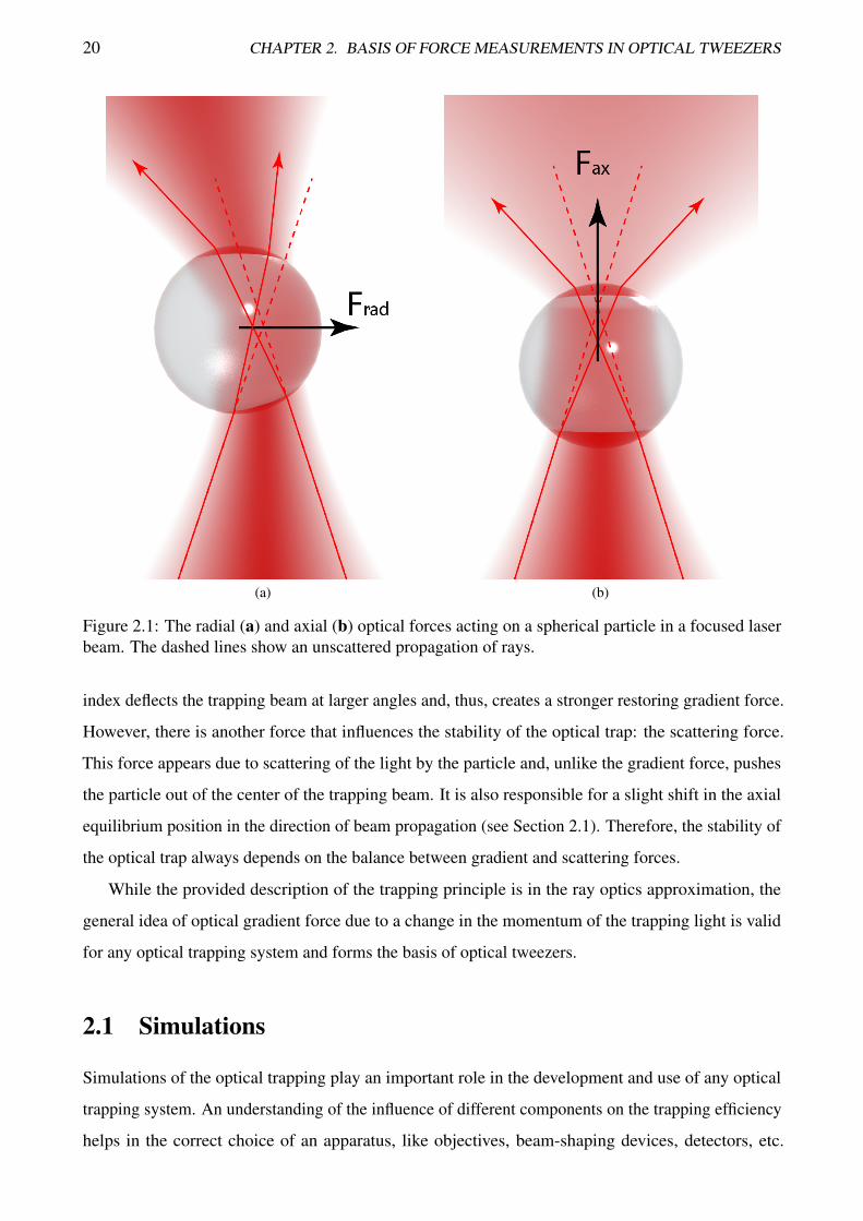
Let’s consider a spherical dielectric particle in a focused beam that has a Gaussian distribution (see
Figure 2.1). When the center of the particle is close to the focus of the trapping light, no optical
force will be exerted on the particle as each ray will fall normally to the surface and will not refract.
If the particle is displaced out of this equilibrium position transverse to the beam propagation axis
(Figure 2.1a), the light will refract, creating a change in the momentum of the light (dashed lines show
the undeflected propagation of the rays). According to the law of conservation of momentum, the
particle will experience a force in the opposite direction. This restoring force will push the particle
back into the equilibrium position. A similar force will appear in the direction of beam propagation
(Figure 2.1b). A variation in the divergence of the beam corresponds to a change in the axial component
of the momentum and will create an axial restoring force which also pushes the particle back into
the equilibrium. Thus, the three-dimensional single beam trapping of a non-absorbing particle can
be achieved by tight focusing of a laser beam. The magnitude of both axial and radial restoring
forces acting on a spherical particle depends on its optical parameters — a higher relative refractive19
20 CHAPTER 2. BASIS OF FORCE MEASUREMENTS IN OPTICAL TWEEZERS
(a) (b)
Figure 2.1: The radial (a) and axial (b) optical forces acting on a spherical particle in a focused laserbeam. The dashed lines show an unscattered propagation of rays.
index deflects the trapping beam at larger angles and, thus, creates a stronger restoring gradient force.
However, there is another force that influences the stability of the optical trap: the scattering force.
This force appears due to scattering of the light by the particle and, unlike the gradient force, pushes
the particle out of the center of the trapping beam. It is also responsible for a slight shift in the axial
equilibrium position in the direction of beam propagation (see Section 2.1). Therefore, the stability of
the optical trap always depends on the balance between gradient and scattering forces.
While the provided description of the trapping principle is in the ray optics approximation, the
general idea of optical gradient force due to a change in the momentum of the trapping light is valid
for any optical trapping system and forms the basis of optical tweezers.
2.1 Simulations
Simulations of the optical trapping play an important role in the development and use of any optical
trapping system. An understanding of the influence of different components on the trapping efficiency
helps in the correct choice of an apparatus, like objectives, beam-shaping devices, detectors, etc.
2.1. SIMULATIONS 21
Simulations are also important for the prediction of experimental outcomes and the correct analysis
of results. As forces in optical tweezers arise from the change in the momentum of the trapping
light, calculations of optical forces require a solution of the scattering problem. In fact, simulation of
optical trapping can be considered as a special case of a more general scattering problem. Except for
a few cases where the scattering can be calculated analytically, it is a complex and computationally
demanding problem to solve. There are a large number of computational methods developed to
accomplish scattering calculations. Accordingly, there are a large number of methods to simulate
an optical trap and calculate forces acting in the system. As three-dimensional trapping requires a
high gradient of intensity, simulations of optical traps are usually performed with focused beams. The
choice of the specific method depends on the geometrical and optical parameters of the particle and the
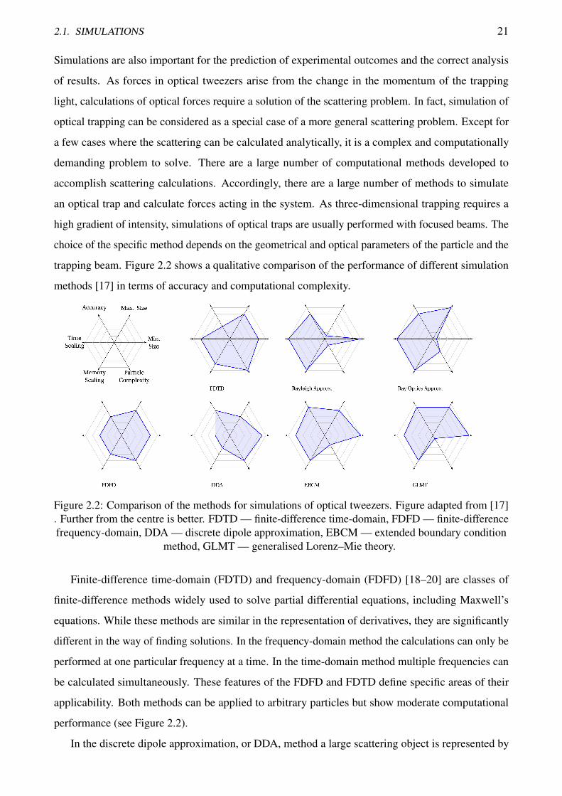
trapping beam. Figure 2.2 shows a qualitative comparison of the performance of different simulation
methods [17] in terms of accuracy and computational complexity.
Figure 2.2: Comparison of the methods for simulations of optical tweezers. Figure adapted from [17]. Further from the centre is better. FDTD — finite-difference time-domain, FDFD — finite-differencefrequency-domain, DDA — discrete dipole approximation, EBCM — extended boundary condition
method, GLMT — generalised Lorenz–Mie theory.
Finite-difference time-domain (FDTD) and frequency-domain (FDFD) [18–20] are classes of
finite-difference methods widely used to solve partial differential equations, including Maxwell’s
equations. While these methods are similar in the representation of derivatives, they are significantly
different in the way of finding solutions. In the frequency-domain method the calculations can only be
performed at one particular frequency at a time. In the time-domain method multiple frequencies can
be calculated simultaneously. These features of the FDFD and FDTD define specific areas of their
applicability. Both methods can be applied to arbitrary particles but show moderate computational
performance (see Figure 2.2).
In the discrete dipole approximation, or DDA, method a large scattering object is represented by
22 CHAPTER 2. BASIS OF FORCE MEASUREMENTS IN OPTICAL TWEEZERS
a number of small discrete dipoles with known polarisability which interact with the field and each
other. With this method the scattering by arbitrary shaped particles can be calculated. However, the
calculations of the scattering for a large particles are both time and memory consuming which makes
it more suitable for calculations for smaller individual particles.
For particles much smaller than the trapping wavelength the Rayleigh approximation can be applied.
In this approximation the particle is considered as a single dipole. The time-averaged gradient force
acting on a spherical Rayleigh particle in an optical gradient ∇I(r) is given by [21]
Fgrad(r) =2πnma3
c
(m2−1m2 +2
)∇I(r) (2.1)
where nm and m are the refractive indices of the surrounding medium and the relative refractive index
of the particle correspondingly, c is the speed of light in vacuum, and a is the radius of the particle.
It is a fast, accurate and memory efficient method for subwavelength particles (a� λ/10) but is
completely inappropriate for calculations of forces acting on bigger particles.
For large particles (relative to the wavelength of trapping beam) the geometrical optics approxi-
mation can be applied. The scattered field can be calculated using ray tracing. There are two main
conditions for this approximation to correctly calculate the scattering field. First, the center of the
beam should be kept away from the surfaces as geometrical optics does not correctly describe the
intensity distribution in the focal spot. Second, the particle should not have small geometrical features
which may create strong interference effects as they will not be appropriately accounted for. If these
requirements are fulfilled, the geometrical optics approximation becomes a powerful time-efficient
tool for optical force calculations. A computational toolbox for optical tweezers in geometrical optics
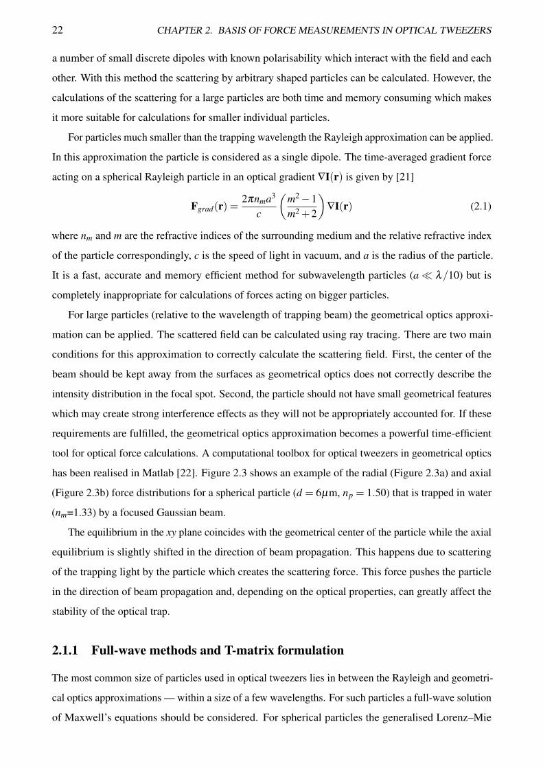
has been realised in Matlab [22]. Figure 2.3 shows an example of the radial (Figure 2.3a) and axial
(Figure 2.3b) force distributions for a spherical particle (d = 6µm, np = 1.50) that is trapped in water
(nm=1.33) by a focused Gaussian beam.
The equilibrium in the xy plane coincides with the geometrical center of the particle while the axial
equilibrium is slightly shifted in the direction of beam propagation. This happens due to scattering
of the trapping light by the particle which creates the scattering force. This force pushes the particle
in the direction of beam propagation and, depending on the optical properties, can greatly affect the
stability of the optical trap.
2.1.1 Full-wave methods and T-matrix formulation
The most common size of particles used in optical tweezers lies in between the Rayleigh and geometri-
cal optics approximations — within a size of a few wavelengths. For such particles a full-wave solution
of Maxwell’s equations should be considered. For spherical particles the generalised Lorenz–Mie
2.1. SIMULATIONS 23
(a) (b)
Figure 2.3: Simulations of the radial (a) and axial (b) forces acting on a spherical particle in thegeometrical optics approximation [22]. The particle (d = 6µm, np = 1.50) is trapped in a Gaussianbeam in water (nm=1.33). The length of the arrows corresponds to the magnitude of force. The shadedarea depicts the particle.
theory (GLMT) [23, 24] effectively describes the scattering process (there are versions of GLMT
for non-spherical particles as well). Therefore, GLMT is usually the best choice when dealing with
spherical objects [17].
An incident and scattered field can be represented in terms of discrete basis sets of functions ψ incn
and ψscatk :
Einc =∞
∑n
anψincn
Escat =∞
∑k
pkψscatk
(2.2)
where an and pk are the expansion coefficients for the incident and scattered waves correspondingly. If
the response of the particle is linear, the relationship between the expansion coefficients will also be
linear and can be written as:
p = Ta (2.3)
where T is a transition matrix (T-matrix), and p and b are vectors of expansion coefficients. Thus, if
the T-matrix of a particle is known, the coefficients of the expansion of the scattered field can be easily
found from the expansion coefficients of the incident wave. The vector spherical wavefunctions can be
24 CHAPTER 2. BASIS OF FORCE MEASUREMENTS IN OPTICAL TWEEZERS
used as a basis to expand the incident and scattered fields [25]:
Einc(kr) =∞
∑n=0
n
∑m=−n
anmM(3)nm(kr)+bnmN(3)
nm(kr),
Escat(kr) =∞
∑n=0
n
∑m=−n
pnmM(1)nm(kr)+qnmN(1)
nm(kr),(2.4)
where M(1,3)nm and N(1,3)
nm are the vector spherical wavefunctions [25]:
M(1,2)nm (kr) = Nnh(1,2)n (kr)Cnm(θ ,φ),
N(1,2)nm (kr) =
h(1,2)n (kr)krNn
Pnm(θ ,φ)+Nn
(h1,2
n−1(kr)− nh(1,2)n (kr)kr
)Bnm(θ ,φ),
M(3) =12
(M(1)+M(2)
),
where h(1,2)n (kr) are spherical Hankel functions of the first (1) and second (2) kind, Nn are normalisation
constants, Cnm(θ ,φ) = ∇× (rY mn (θ ,φ)), Pnm(θ ,φ) = rY m
n (θ ,φ), Bnm(θ ,φ) = r∇Y mn (θ ,φ) are the
vector spherical harmonics expressed in terms of normalised scalar spherical harmonics Y mn (θ ,φ), r,
θ and φ are radial distance, polar and azimuthal angles correspondingly, k is the wavevector of the
beam. While these expansions of the fields contain an infinite number of terms, in practice a series
will be truncated at some nmax. The nmax depends on the parameters of the trapping beam and the
size of a particle. As a general rule, it can be calculated as nmax = kr0 +3 3√
3kr0, where r0 is a radius
of the scatterer [26]. For a given particle, the T-matrix depends only on its parameters and not on
the parameters of trapping beam. There are methods to perform rotations and translations [27–29]
of the T-matrix which gives the ability to use it for different locations and orientations of the particle
in the trap. This makes possible computationally efficient simulations of the dynamics of a trapped
object. While generalised Lorenz–Mie theory can be used to calculate a T-matrix for a spherical
particle, the extended boundary condition method (EBCM) was developed as a method of calculating a
T-matrix [30] for non-spherical particles. However, the EBCM is restricted to isotropic homogeneous
particles as the field within the particle is expanded into regular vector spherical wavefunctions. In
principle, any of the methods described here can be used to calculate a T-matrix and the choice of
a particular method depends on the particle size and complexity. The use of a T-matrix method is
justified when it can be reused, for example in simulations of Brownian motion of a particle in the trap.
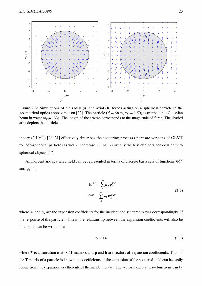
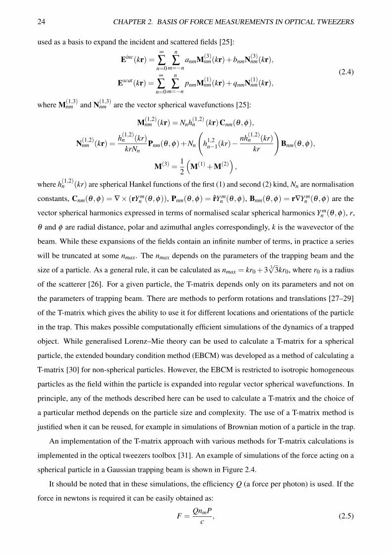
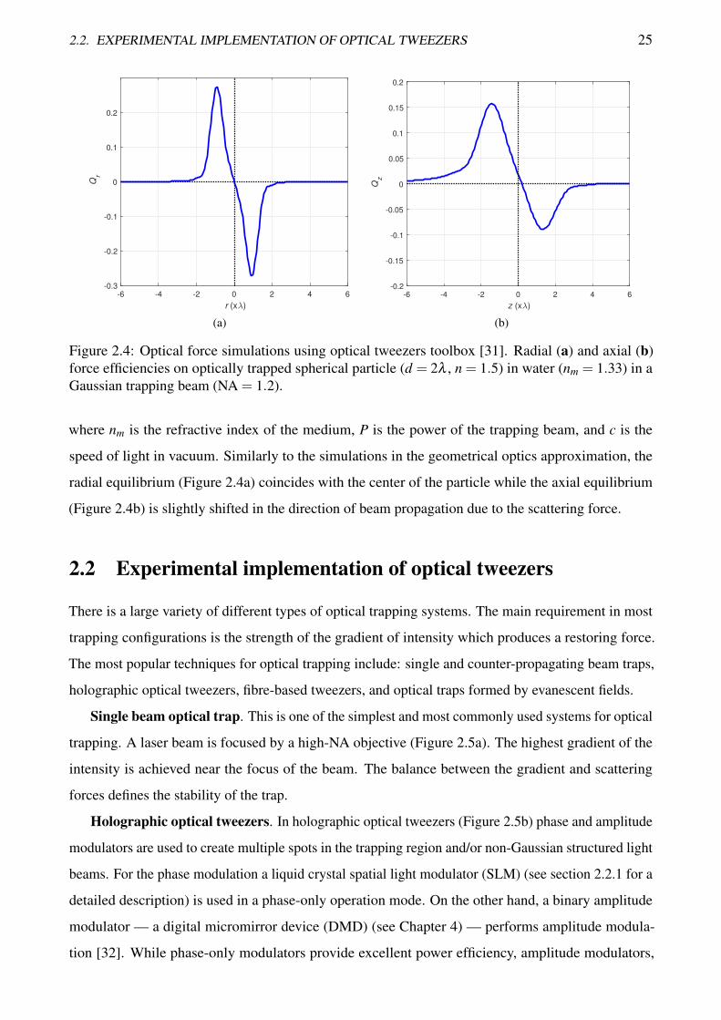
An implementation of the T-matrix approach with various methods for T-matrix calculations is
implemented in the optical tweezers toolbox [31]. An example of simulations of the force acting on a
spherical particle in a Gaussian trapping beam is shown in Figure 2.4.
It should be noted that in these simulations, the efficiency Q (a force per photon) is used. If the
force in newtons is required it can be easily obtained as:
F =QnmP
c, (2.5)
2.2. EXPERIMENTAL IMPLEMENTATION OF OPTICAL TWEEZERS 25
-6 -4 -2 0 2 4 6
r (x )
-0.3
-0.2
-0.1
0
0.1
0.2
Qr
(a)
-6 -4 -2 0 2 4 6
z (x )
-0.2
-0.15
-0.1
-0.05
0
0.05
0.1
0.15
0.2
Qz
(b)
Figure 2.4: Optical force simulations using optical tweezers toolbox [31]. Radial (a) and axial (b)force efficiencies on optically trapped spherical particle (d = 2λ , n = 1.5) in water (nm = 1.33) in aGaussian trapping beam (NA = 1.2).
where nm is the refractive index of the medium, P is the power of the trapping beam, and c is the
speed of light in vacuum. Similarly to the simulations in the geometrical optics approximation, the
radial equilibrium (Figure 2.4a) coincides with the center of the particle while the axial equilibrium
(Figure 2.4b) is slightly shifted in the direction of beam propagation due to the scattering force.
2.2 Experimental implementation of optical tweezers
There is a large variety of different types of optical trapping systems. The main requirement in most
trapping configurations is the strength of the gradient of intensity which produces a restoring force.
The most popular techniques for optical trapping include: single and counter-propagating beam traps,
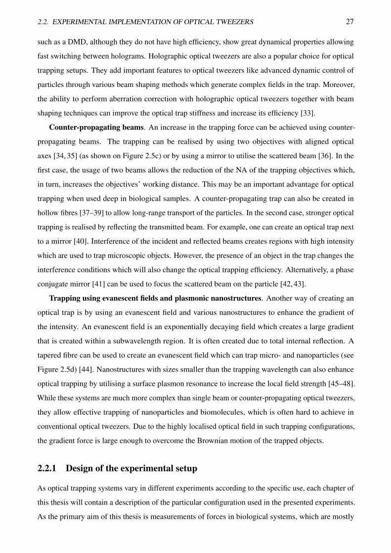
holographic optical tweezers, fibre-based tweezers, and optical traps formed by evanescent fields.
Single beam optical trap. This is one of the simplest and most commonly used systems for optical
trapping. A laser beam is focused by a high-NA objective (Figure 2.5a). The highest gradient of the
intensity is achieved near the focus of the beam. The balance between the gradient and scattering
forces defines the stability of the trap.
Holographic optical tweezers. In holographic optical tweezers (Figure 2.5b) phase and amplitude
modulators are used to create multiple spots in the trapping region and/or non-Gaussian structured light
beams. For the phase modulation a liquid crystal spatial light modulator (SLM) (see section 2.2.1 for a
detailed description) is used in a phase-only operation mode. On the other hand, a binary amplitude
modulator — a digital micromirror device (DMD) (see Chapter 4) — performs amplitude modula-
tion [32]. While phase-only modulators provide excellent power efficiency, amplitude modulators,

26 CHAPTER 2. BASIS OF FORCE MEASUREMENTS IN OPTICAL TWEEZERS
(a) (b) (c)
(d)
(e)
Figure 2.5: Optical trapping configurations. (a) Single beam optical trap. (b) Holographic opticaltweezers. A diffraction element is used to create multiple traps. (c) Counter-propagating trap createdwith two objectives. (d) Tapered optical fibre creates an optical trap in evanescent field. (e) Doublenanoholes structure creates an optical gradient at the sharp edges when illuminated. These images arefor illustration purposes only and do not include an accurate intensity distribution.
2.2. EXPERIMENTAL IMPLEMENTATION OF OPTICAL TWEEZERS 27
such as a DMD, although they do not have high efficiency, show great dynamical properties allowing
fast switching between holograms. Holographic optical tweezers are also a popular choice for optical
trapping setups. They add important features to optical tweezers like advanced dynamic control of
particles through various beam shaping methods which generate complex fields in the trap. Moreover,
the ability to perform aberration correction with holographic optical tweezers together with beam
shaping techniques can improve the optical trap stiffness and increase its efficiency [33].
Counter-propagating beams. An increase in the trapping force can be achieved using counter-
propagating beams. The trapping can be realised by using two objectives with aligned optical
axes [34, 35] (as shown on Figure 2.5c) or by using a mirror to utilise the scattered beam [36]. In the
first case, the usage of two beams allows the reduction of the NA of the trapping objectives which,
in turn, increases the objectives’ working distance. This may be an important advantage for optical
trapping when used deep in biological samples. A counter-propagating trap can also be created in
hollow fibres [37–39] to allow long-range transport of the particles. In the second case, stronger optical
trapping is realised by reflecting the transmitted beam. For example, one can create an optical trap next
to a mirror [40]. Interference of the incident and reflected beams creates regions with high intensity
which are used to trap microscopic objects. However, the presence of an object in the trap changes the
interference conditions which will also change the optical trapping efficiency. Alternatively, a phase
conjugate mirror [41] can be used to focus the scattered beam on the particle [42, 43].
Trapping using evanescent fields and plasmonic nanostructures. Another way of creating an
optical trap is by using an evanescent field and various nanostructures to enhance the gradient of
the intensity. An evanescent field is an exponentially decaying field which creates a large gradient
that is created within a subwavelength region. It is often created due to total internal reflection. A
tapered fibre can be used to create an evanescent field which can trap micro- and nanoparticles (see
Figure 2.5d) [44]. Nanostructures with sizes smaller than the trapping wavelength can also enhance
optical trapping by utilising a surface plasmon resonance to increase the local field strength [45–48].
While these systems are much more complex than single beam or counter-propagating optical tweezers,
they allow effective trapping of nanoparticles and biomolecules, which is often hard to achieve in
conventional optical tweezers. Due to the highly localised optical field in such trapping configurations,
the gradient force is large enough to overcome the Brownian motion of the trapped objects.
2.2.1 Design of the experimental setup
As optical trapping systems vary in different experiments according to the specific use, each chapter of
this thesis will contain a description of the particular configuration used in the presented experiments.
As the primary aim of this thesis is measurements of forces in biological systems, which are mostly
28 CHAPTER 2. BASIS OF FORCE MEASUREMENTS IN OPTICAL TWEEZERS
in a micron range of sizes, three-dimensional single and multi-beam optical trapping systems with
holographic control of the beam are used. This section will contain a description of common elements
which are present in most of the performed experiments.
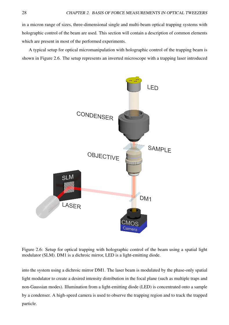
A typical setup for optical micromanipulation with holographic control of the trapping beam is
shown in Figure 2.6. The setup represents an inverted microscope with a trapping laser introduced
Figure 2.6: Setup for optical trapping with holographic control of the beam using a spatial lightmodulator (SLM). DM1 is a dichroic mirror, LED is a light-emitting diode.
into the system using a dichroic mirror DM1. The laser beam is modulated by the phase-only spatial
light modulator to create a desired intensity distribution in the focal plane (such as multiple traps and
non-Gaussian modes). Illumination from a light-emitting diode (LED) is concentrated onto a sample
by a condenser. A high-speed camera is used to observe the trapping region and to track the trapped
particle.
2.2. EXPERIMENTAL IMPLEMENTATION OF OPTICAL TWEEZERS 29
The choice of the trapping wavelength depends on the specific applications, but commonly a
wavelength of 1064nm is used — an infrared emission line of the widely used neodymium-doped
yttrium aluminium garnet (Nd:YAG) laser. This wavelength lies within the near-infrared optical
window in biological tissues which makes optical tweezers suitable for biological experiments by
avoiding overheating in the trap and maximising the penetration depth of the laser beam. In fact, a
wavelength of 800–900nm is usually a better choice for biological systems as the absorption in this
range is even smaller, but the lasers (usually Ti:sapphire) are less common (but still widely used).
Control of the beam is performed with a spatial light modulator (SLM) — a liquid crystal-based
device. An SLM consists of an array of cells with electrodes. As the electric field changes, the
molecules of the nematic liquid crystal reorient in the cell and align along the lines of electric field.
Such a system acts as an uniaxial crystal with an electrically controlled orientation of the optical axes
and thus, control of the refractive index for a given linearly polarised light. Therefore, SLMs are
able to produce a phase modulation of the incoming beam by individual control of each pixel in the
array. To transfer the phase modulation into amplitude variations in the trapping region, phase-only
modulators are used in a Fourier plane of the lens (which often coincides with a focal plane). In optical
trapping systems, the objective is a Fourier transforming lens which creates a desired light distribution
in the sample. The advantage of phase-only modulators for optical trapping over amplitude modulators
is in significantly higher power efficiency as the light is not absorbed or deflected but redirected into
required locations with high diffraction efficiency.
The objective is the most important part in the design of the system. Usually a high-NA objective
is required to achieve three-dimensional trapping. Various aberrations in the optical systems distort the
optical beam and decrease its performance. While a spatial light modulator is capable of correcting
most of the aberrations, it is desirable to minimise these aberrations in the design of the system. The
trapping region is the most vulnerable to aberrations part as it is created by a high-NA objective and
contains several layers of different materials which form a sample chamber. If the trapping is performed
mostly in water (or in a medium with a similar refractive index), a water immersion objective will
show the best performance due to the match in refractive indices of immersion liquid and trapping
medium. This allows trapping deep in the sample without significant distortions of beam in the focal
region [49].
Visual control of experiments is performed by imaging the sample onto a camera. Tracking of
the trapped objects can be realised with position sensors such as a quadrant photodetector and lateral
position sensitive detectors (see Chapter 3 for more details). However, the particle can be tracked
directly using the imaging camera. To achieve a bandwidth of 5–10kHz for the position detection
a high-speed camera is used. The experiments in this chapter are performed on spherical particles;
30 CHAPTER 2. BASIS OF FORCE MEASUREMENTS IN OPTICAL TWEEZERS
therefore, we can restrict the algorithm of the image recognition to spherical objects. Other algorithms
for determination of the position of non-spherical particles will be introduced in the later chapters.
The most straightforward way to find the position of a spherical particle is to calculate the centroid of
the whole image. However, the background of the image should be removed prior to the calculations
by setting a threshold level; otherwise, any bright object that appears in the background will change
the calculated centroid dramatically. A different and more complex algorithm can be found in [50].
This algorithm calculates the centroid by finding the best-fit radial symmetry center. It depends on the
gradient of the intensity and thus can be used for images with non-zero background.
As the aim of this thesis is an investigation of force measurements in biological systems, the
optical setup was designed to fit the requirements of such systems. An ytterbium doped fibre laser
(YLR-10-1064-LP, 10W, 1064nm, IPG Photonics) and a high-NA objective (Olympus UPlanSApo
60×, water immersion, 1.2 NA) are used to ensure low absorption and to obtain minimal aberrations
in the trapping region. The position measurement was performed using a high-speed CMOS camera
(Mikrotron MC1362, 1280× 1024), running at 5000 frames per second. The radial displacements
of the particle was determined by tracking the position of the centroid of the particle through image
analysis.
2.3 Force measurements
The most common method of force measurement in optical tweezers is through position detection.
When a particle is trapped within a linear region of the force, we can assume that the trap is Hookean
and can be characterised by a spring constant k:
Fx =−kx, (2.6)
where x is the displacement of the particle from the equilibrium. Thus, if the trap stiffness k is known,
we can measure the displacement of the particle and calculate the force. To find the trap stiffness of
the optical trap we need to perform a calibration by using another known force, e.g., viscous drag
force, statistics of Brownian motion, etc. It should be noted that this calibration will be specific to each
particle, surrounding medium, and trapping beam, and recalibration will be required if one of those has
changed. There are a number of methods to perform this calibration. Below, the description of the most
popular methods of calibration is given: using the equipartition theorem and Boltzmann statistics [51],
by analysing the power spectrum [52, 53], and finally, by using drag force measurements [54, 55].
Another method for optical force measurements by detection of the change of the momentum of
the scattered light will be described in details in Chapter 3.
2.3. FORCE MEASUREMENTS 31
2.3.1 Equipartition theorem
The equipartition theorem [56–58] states that in a physical system at thermal equilibrium the energy is
equally distributed among the degrees of freedom and equal to 1/2kBT per degree of freedom (kB is
the Boltzmann constant, and T is the absolute temperature of the system). Thus, the calibration of the
optical trap can be performed using the statistical distribution of the position of the particle in the trap.
Assuming that the optical trap is linear:
12
k〈x2〉= 12
kBT −→ k =kBT〈x2〉
, (2.7)
where k is the stiffness of the optical trap, x is the displacement, and 〈x2〉 is the variance of the
position of the particle. This method is independent of the size of the trapped particle, viscosity
of the medium and not sensitive to small fluctuations in the temperature. However, the noise in
the measurement system increases the measured distribution of the displacement of the particle and
therefore, underestimates the trap stiffness [59].
2.3.2 Power spectrum
In a power spectrum calibration method the trap stiffness is estimated from the predicted power
spectrum of the position of the particle in the optical trap. There are two types of calibration methods
using the power spectrum [60]: passive [52, 61] and active [62, 63]. In a passive calibration method
the optically trapped particle undergoes only Brownian motion which is described by the Langevin
equation [64]:
md2xdt2 =−γ
dxdt− kx(t)+
√2kBT γ W (t) , (2.8)
where m is the mass of the trapped particle, x is its position, γ is the damping coefficient (γ = 6πµR for
a spherical particle with a radius R in a liquid with a dynamic viscosity µ),√
2kBT γ W (t) represents
a random Brownian force. As the characteristic time of the loss of kinetic energy of the particle is very
low, the inertial term md2xdt2 in equation 2.8 can be dropped [52]:
dxdt
+2π fcx(t) =
√2kBT
γW (t) , (2.9)
where fc ≡ k/(2πγ) is a corner frequency.
The power spectrum Sx( f ) of the position of the trapped particle is described by a Lorentzian
function [65]:
Sx( f ) =kBT
2γπ2 ( f 2c + f 2)
. (2.10)
where f is the frequency in hertz.
32 CHAPTER 2. BASIS OF FORCE MEASUREMENTS IN OPTICAL TWEEZERS
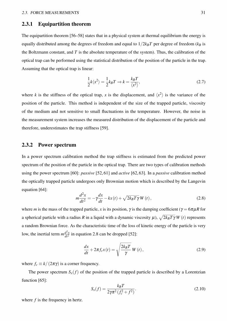
Thus, the corner frequency (and accordingly the trap stiffness) can be found by fitting a Lorentzian
function to the measured power spectrum of the position distribution of the particle. A detailed
description of the method, including discussion on the aliasing and cross-talk in the detection system,
can be found in [52] and [61]. Figure 2.7 shows a power spectrum of a trapped silica particle
(d = 1.7µm) in water (µ = 0.9mPa · s). The calibration constant can be found using a Matlab program
101 102 103 104
Frequency, [Hz]
10-8
10-7
10-6
10-5
10-4
10-3
Po
we
r sp
ectr
um
, [a
rb.
un
its]
fc = 54.1 1.4 Hz
k = 4.93 0.13 pN/ m
Experimental data
Lorentzian
Figure 2.7: Calibration of the optical trap using the power spectrum method [52]. The corner frequencyis estimated from the Lorentzian fit (equation 2.10). The trap stiffness is calculated (see equation 2.9)from the parameters of the trapped spherical particle (silica, d = 1.7µm in water, µ = 0.9mPa · s)
available in reference [66] which includes cross-talk, aliasing and low-pass filtering corrections.
The usage of a frequency space for the determination of the trap stiffness has the advantage
of the possibility to remove some resonant frequencies (e.g., stage oscillations). Also, the power
spectrum method is less sensitive to noise in the measurements than the equipartition method. However,
knowledge of the size of the particle and the viscosity of the medium is required. This method is
also sensitive to temperature changes (through the temperature dependence of the viscosity) and the
presence of other surfaces (which also influence the viscosity).
Most of the disadvantages of the passive method can be overcome by using the active calibration
method. In this method, instead of measuring the thermal motion, an external sinusoidal force is
applied to oscillate the particle in the trap (by moving either the stage, or the trapping beam). The
2.3. FORCE MEASUREMENTS 33
power spectrum of the position of the particle becomes [53]:
Sx( f ) =kBT
γπ2 ( f 2c + f 2)
+A2
2(1+ f 2
c / f 2drive
)δ ( f − fdrive) , (2.11)
where A and fdrive are the amplitude and frequency of the oscillation respectively. Thus, the corner
frequency can be found by measuring the power at the driving frequency (the second term in equa-
tion 2.11). The viscosity of the medium is estimated by fitting a Lorentzian function to the power
spectrum. Then, the trap stiffness is calculated as:
k = 2πγ fc. (2.12)
As both the viscosity γ and corner frequency fc are determined simultaneously, the active calibration
method does not require prior knowledge of the viscosity.
2.3.3 Boltzmann statistics
The Boltzmann statistics method relies on calculations of the potential of the optical trap from the
position distribution of the particle. Boltzmann statistics describes the probability of finding a particle
in a scalar potential U(x) at the equilibrium temperature T as [67]:
p(x) =1Z
e−U(x)kBT , (2.13)
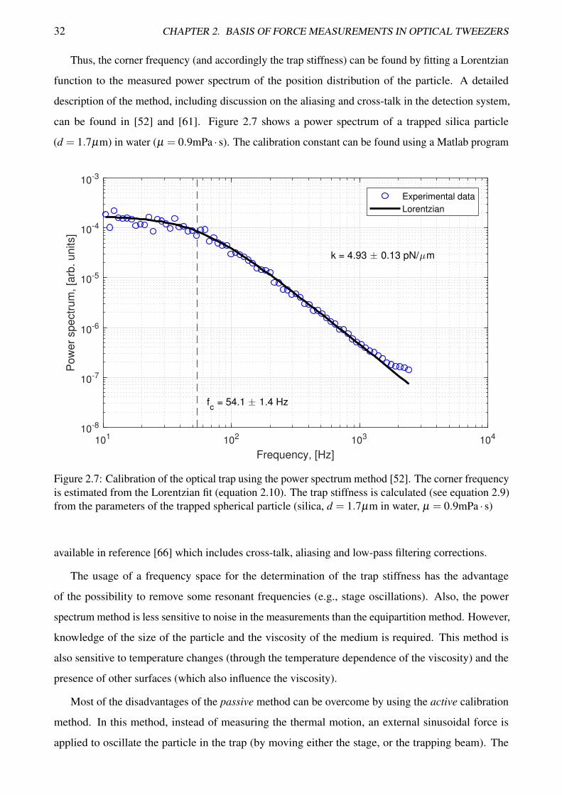
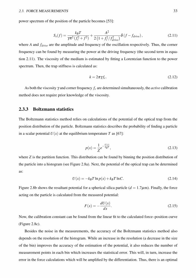
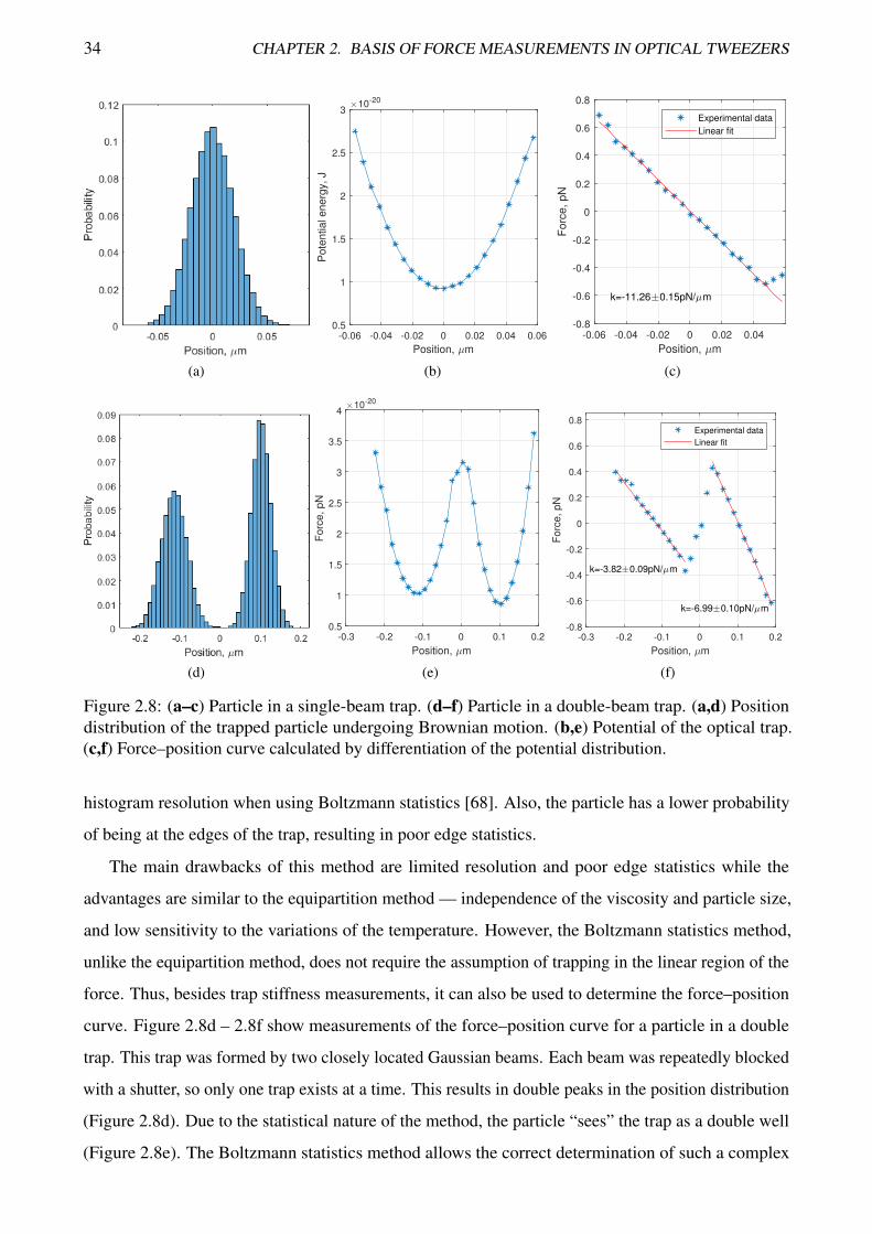
where Z is the partition function. This distribution can be found by binning the position distribution of
the particle into a histogram (see Figure 2.8a). Next, the potential of the optical trap can be determined
as:
U(x) =−kBT ln p(x)+ kBT lnC. (2.14)
Figure 2.8b shows the resultant potential for a spherical silica particle (d = 1.7µm). Finally, the force
acting on the particle is calculated from the measured potential:
F(x) =−dU(x)dx
. (2.15)
Now, the calibration constant can be found from the linear fit to the calculated force–position curve
(Figure 2.8c).
Besides the noise in the measurements, the accuracy of the Boltzmann statistics method also
depends on the resolution of the histogram. While an increase in the resolution (a decrease in the size
of the bin) improves the accuracy of the estimation of the potential, it also reduces the number of
measurement points in each bin which increases the statistical error. This will, in turn, increase the
error in the force calculations which will be amplified by the differentiation. Thus, there is an optimal
34 CHAPTER 2. BASIS OF FORCE MEASUREMENTS IN OPTICAL TWEEZERS
(a)
-0.06 -0.04 -0.02 0 0.02 0.04 0.06
Position, m
0.5
1
1.5
2
2.5
3
Po
ten
tia
l e
ne
rgy,
J
10-20
(b)
-0.06 -0.04 -0.02 0 0.02 0.04
Position, m
-0.8
-0.6
-0.4
-0.2
0
0.2
0.4
0.6
0.8
Forc
e, pN
k=-11.26 0.15pN/ m
Experimental data
Linear fit
(c)
(d)
-0.3 -0.2 -0.1 0 0.1 0.2
Position, m
0.5
1
1.5
2
2.5
3
3.5
4
Fo
rce
, p
N
10-20
(e)
-0.3 -0.2 -0.1 0 0.1 0.2
Position, m
-0.8
-0.6
-0.4
-0.2
0
0.2
0.4
0.6
0.8
Fo
rce
, p
N
k=-3.82 0.09pN/ m
k=-6.99 0.10pN/ m
Experimental data
Linear fit
(f)
Figure 2.8: (a–c) Particle in a single-beam trap. (d–f) Particle in a double-beam trap. (a,d) Positiondistribution of the trapped particle undergoing Brownian motion. (b,e) Potential of the optical trap.(c,f) Force–position curve calculated by differentiation of the potential distribution.
histogram resolution when using Boltzmann statistics [68]. Also, the particle has a lower probability
of being at the edges of the trap, resulting in poor edge statistics.
The main drawbacks of this method are limited resolution and poor edge statistics while the
advantages are similar to the equipartition method — independence of the viscosity and particle size,
and low sensitivity to the variations of the temperature. However, the Boltzmann statistics method,
unlike the equipartition method, does not require the assumption of trapping in the linear region of the
force. Thus, besides trap stiffness measurements, it can also be used to determine the force–position
curve. Figure 2.8d – 2.8f show measurements of the force–position curve for a particle in a double
trap. This trap was formed by two closely located Gaussian beams. Each beam was repeatedly blocked
with a shutter, so only one trap exists at a time. This results in double peaks in the position distribution
(Figure 2.8d). Due to the statistical nature of the method, the particle “sees” the trap as a double well
(Figure 2.8e). The Boltzmann statistics method allows the correct determination of such a complex

2.3. FORCE MEASUREMENTS 35
force field and the stiffnesses of both traps can be determined (Figure 2.8f). It should be noted that the
force measured with this method corresponds to the total force acting on the particle. While a constant
force will appear as a shift of the potential distribution, a changing force will distort the potential and,
thus, the measured force. Therefore, all forces with sufficient gradient within the range of the thermal
motion of the trapped particle should be avoided.
2.3.4 Drag force
A fluid drag force can be used to calibrate the optical trap. A spherical particle in a Stokes flow
experiences a drag force:
Fdrag =−6πµRV, (2.16)
where µ is the viscosity of medium, R is the radius of particle, and V is the velocity of the trapped
particle relative to the fluid. The drag force shifts the particle out of the equilibrium point (Figure 2.9a).
This calibration method requires a piezo or motorised stage to apply a drag force using a constant flow
(a)
0 1 2 3 4 5 6 7 8
Time, [s]
-0.15
-0.1
-0.05
0
0.05
0.1
0.15
0.2
0.25
0.3
0.35
Dis
pla
cem
ent, [
m]
x=0.23 m
(b)
Figure 2.9: Drag force calibration method. (a) Trapping geometry. Particle is displaced out of theequilibrium by the fluid drag force (b) Position of the particle in the optical trap.
of the liquid. If particle remains in the linear region of the optical force and all the parameters in the
equation 2.16 are known, the trap stiffness can be found by measuring the displacement of the particle:
k =−Fdrag
∆x=
6πµRV∆x
. (2.17)
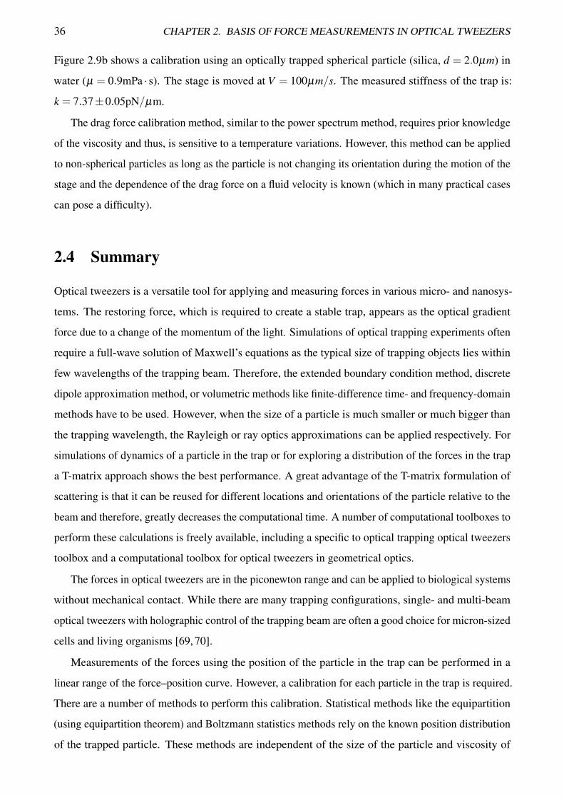
36 CHAPTER 2. BASIS OF FORCE MEASUREMENTS IN OPTICAL TWEEZERS
Figure 2.9b shows a calibration using an optically trapped spherical particle (silica, d = 2.0µm) in
water (µ = 0.9mPa · s). The stage is moved at V = 100µm/s. The measured stiffness of the trap is:
k = 7.37±0.05pN/µm.
The drag force calibration method, similar to the power spectrum method, requires prior knowledge
of the viscosity and thus, is sensitive to a temperature variations. However, this method can be applied
to non-spherical particles as long as the particle is not changing its orientation during the motion of the
stage and the dependence of the drag force on a fluid velocity is known (which in many practical cases
can pose a difficulty).
2.4 Summary
Optical tweezers is a versatile tool for applying and measuring forces in various micro- and nanosys-
tems. The restoring force, which is required to create a stable trap, appears as the optical gradient
force due to a change of the momentum of the light. Simulations of optical trapping experiments often
require a full-wave solution of Maxwell’s equations as the typical size of trapping objects lies within
few wavelengths of the trapping beam. Therefore, the extended boundary condition method, discrete
dipole approximation method, or volumetric methods like finite-difference time- and frequency-domain
methods have to be used. However, when the size of a particle is much smaller or much bigger than
the trapping wavelength, the Rayleigh or ray optics approximations can be applied respectively. For
simulations of dynamics of a particle in the trap or for exploring a distribution of the forces in the trap
a T-matrix approach shows the best performance. A great advantage of the T-matrix formulation of
scattering is that it can be reused for different locations and orientations of the particle relative to the
beam and therefore, greatly decreases the computational time. A number of computational toolboxes to
perform these calculations is freely available, including a specific to optical trapping optical tweezers
toolbox and a computational toolbox for optical tweezers in geometrical optics.
The forces in optical tweezers are in the piconewton range and can be applied to biological systems
without mechanical contact. While there are many trapping configurations, single- and multi-beam
optical tweezers with holographic control of the trapping beam are often a good choice for micron-sized
cells and living organisms [69, 70].
Measurements of the forces using the position of the particle in the trap can be performed in a
linear range of the force–position curve. However, a calibration for each particle in the trap is required.
There are a number of methods to perform this calibration. Statistical methods like the equipartition
(using equipartition theorem) and Boltzmann statistics methods rely on the known position distribution
of the trapped particle. These methods are independent of the size of the particle and viscosity of
2.4. SUMMARY 37
the medium. However, being statistical methods, they are vulnerable to noise in the measurement
system which may lead to an underestimation of the trap stiffness. In the power spectrum method
some sources of the noise can be suppressed as calculations are performed in the frequency domain.
Unlike the statistical methods, the power spectrum method requires prior knowledge of the viscosity
of the medium and, therefore, is very sensitive to small variations in the temperature. Alternatively, a
drag force can be utilised to perform the calibration. The final decision on the particular calibration
method of the optical trap depends on the particular properties of the experiment.

The following publication has been incorporated as Chapter 3.
1. A. A. M. Bui, A. V. Kashchuk, M. A. Balanant, T. A. Nieminen, H. Rubinsztein-Dunlop, and A. B.
Stilgoe. Calibration of force detection for arbitrarily shaped particles in optical tweezers. Scientific
Reports 8(1), 10798, 2018
Contributor Statement of contribution %A. A. M. Bui conception and design 20
preparation of text and figures 30analysis and interpretation 30numerical calculations 100
A. V. Kashchuk conception and design 20performed experiments 90analysis and interpretation 40preparation of text and figures 30
M. A. Balanant preparation of RBCs samples 100T. A. Nieminen conception and design 20
preparation of text and figures 30analysis and interpretation 10supervision, guidance 30
H. Rubinsztein-Dunlop conception and design 20supervision, guidance 30analysis and interpretation 10preparation of text and figures 5
A. B. Stilgoe conception and design 20performed experiments 10supervision, guidance 40analysis and interpretation 10preparation of text and figures 5

Chapter 3
Direct optical force measurements
3.1 Introduction
The methods for the force measurements introduced in the Chapter 2 — power spectrum method,
equipartition method and drag force calibration — are based on the determination of the trap stiffness
using position measurements. However, to convert the position of the trapped object into a force, a
calibration is required. This involves a measurement of the trap stiffness for each particle, beam shape
and trapping medium. Moreover, such methods assume a linear dependence of the force with the
position of the trapped particle and thus, are restricted mostly to small displacements.
Another method is to measure the change in the momentum of the light scattered by the particle
[34, 71]. The optical gradient force arises from deflection of the transmitted beam by the particle. This
changes the momentum flux of the beam, which, by conservation of momentum, results in an optical
force acting on the particle [2]. The important requirement for exact measurement is the collection
of all of the scattered light, but in practice, it is not feasible to collect the light at all possible angles.
However, it was shown that for most particles used in optical tweezers, light is mainly scattered in the
forward direction [72] and a condenser with a high numerical aperture will be able to collect most of
this light. Also, the accuracy can be improved by detecting the back-scattered light which is especially
important for the determination of the axial force [73]. Alternatively, a dual-beam optical trapping
system [34] can use low-NA objectives which reduce the scattering at large angles. As this method is
based on the detection of the momentum of the light, it is independent of the physical properties of
particles or media used and thus calibration-free.
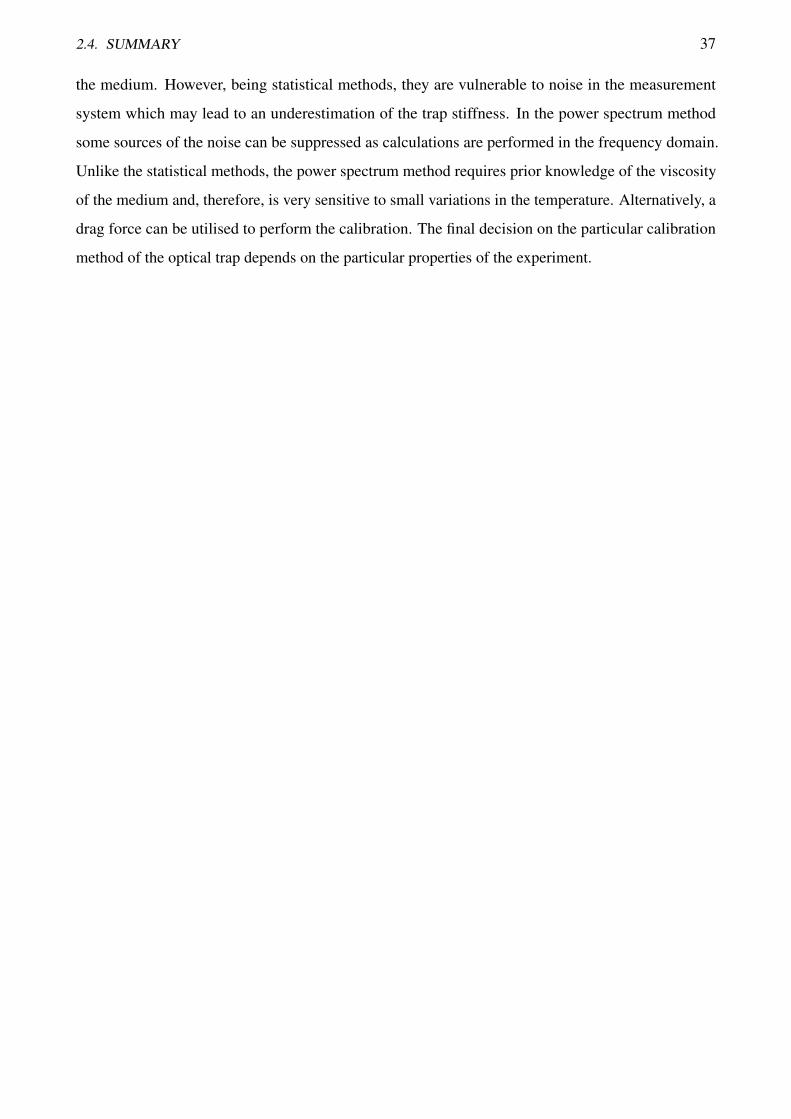
Let us consider an optical trap formed by an objective lens (Figure 3.1). The scattered light is
collected by the condenser lens. The components of the momentum of a ray which is scattered at a39
40 CHAPTER 3. DIRECT OPTICAL FORCE MEASUREMENTS
polar angle θ and azimuthal angle φ are:
p =
px
py
pz
=
psinθ cosφ
psinθ sinφ
pcosθ
= p
x
CA
yCA√
1− x2+y2
C2A
, (3.1)
where CA = r/sinθ is a constant of the condenser (Abbe sine condition), r is a radial distance
from the optical axis in the BFP, x and y are coordinates in the back focal plane (BFP).
BFP
pp
r
θ φ
y
x
Objective Condenser
Figure 3.1: Scheme of the direct force measurement. The sample chamber is omitted for clarity. Theangular distribution of the scattered light is transferred to the transverse distribution in the back focalplane (BFP) by the condenser lens.
Unlike the paraxial ray optics approximation, for a real optical system (which often includes a
high NA condenser and objective) the mapping of the angular distribution of the scattered light to the
transverse distribution is not maintained for an arbitrary plane. However, if the condenser satisfies the
Abbe sine condition [74] (which is the case for the objectives with correction for spherical aberrations),
the mapping will be correct in the BFP of the condenser. Thus, the force, F, can be determined from
the light distribution in the BFP of the condenser by integrating over all collected rays [73]:
F =
Fx
Fy
Fz
=HCA
∫∫
I(x,y)xdxdy∫∫I(x,y)ydxdy∫∫
I(x,y)√
C2A− (x2 + y2) dxdy
−F0, (3.2)
where I(x,y) is the light intensity distribution in the detector’s plane, H is the constant which includes
magnification of the optical system and all absorptions/reflections in the optical elements, and F0
corresponds to the momentum flux of an empty trap [34, 71–73].
3.2. DETECTORS FOR DIRECT OPTICAL FORCE MEASUREMENTS 41
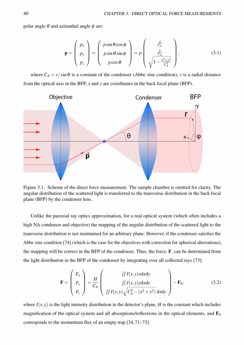
(a) (b) (c)
Figure 3.2: Position detectors: (a) Duo-lateral position sensitive detector (PSD). (b) Quadrant pho-todetector (QPD). (c) Camera.
By definition, the (normalised) centroid of the pattern is:
(X ;Y ) =(∫∫
I(x,y)xdxdy∫∫I(x,y)dxdy
;∫∫
I(x,y)ydxdy∫∫I(x,y)dxdy
). (3.3)
The radial components of the force (x and y) are proportional to the unnormalised centroid (i.e. the
numerator in the equation 3.3) of the pattern (see equation (3.2)) which is proportional to the total
power of the beam.
As can be seen from equation (3.3), the information about the position is contained in the numerator
and the denominator represents the total power which is position independent. Thus, to measure
the radial optical forces, position detectors are used. The detector has to generate a signal S ∝∫∫I(x,y)xdxdy. The light filtered by this linear modulation is also proportional to the unnormalised
centroid of the pattern P−∫∫
I(x,y)xdxdy, where P is the total power of the beam, so often, to obtain
the maximum signal-to-noise ratio, both signals are measured and subtracted. The input signal of the
centered beam is divided into two equal parts with each part proportional to the displacement of the
beam but with opposite signs. When the beam is moved out of the center of the detector, the balance
between the parts is also changing proportionally to the displacement.
3.2 Detectors for direct optical force measurements
There are three types of position detectors which may be potentially used for such direct force
measurements: position sensitive detectors (PSDs), split detectors (SD) and cameras (Figure 3.2).
3.2.1 Position Sensitive Detectors
The position sensitive detector (PSD) consists of a photodetector with resistive layers on the front
(tetra-lateral) [75, 76] or both front and back (duo-lateral) [77] sides (Figure 3.2a). The position
measurements along one axis requires a set of two electrodes placed near the opposite edges of a
42 CHAPTER 3. DIRECT OPTICAL FORCE MEASUREMENTS
rectangular photodiode [78]. In these devices, the measured signal at each electrode is proportional
to the photoresistance current that changes as a function of position. Another set of two electrodes
near the orthogonal edges allows the measurements in two axes simultaneously. The output from the
detector is:
SPSD = S+PSD−S−PSD = ℜGL∫∫−L
I(x,y)xdxdy, (3.4)
where 2L is the length of the detector, S+PSD and S−PSD are signals from the electrodes on the opposite
sides of the detector, ℜ and G are the responsivity and transimpedance gain of the detector, respectively.
These detectors are relatively slow (the bandwidth is typically on the order of tens of kHz) due to
large surface areas, but provide excellent linearity and the output is independent of the spot shape and
size [79]. This makes these detectors an excellent choice for direct force measurement in the directions
transverse to the beam propagation.
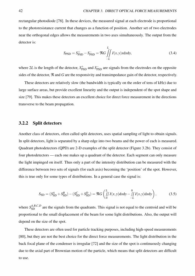
3.2.2 Split detectors
Another class of detectors, often called split detectors, uses spatial sampling of light to obtain signals.
In split detectors, light is separated by a sharp edge into two beams and the power of each is measured.
Quadrant photodetectors (QPD) are 2-D examples of the split detector (Figure 3.2b). They consist of
four photodetectors — each one makes up a quadrant of the detector. Each segment can only measure
the light impinged on itself. Thus only a part of the intensity distribution can be measured with the
difference between two sets of signals (for each axis) becoming the ‘position’ of the spot. However,
this is true only for some types of distributions. In a general case the signal is:
SSD = (SASD +SB
SD)− (SCSD +SD
SD) = ℜG(
L∫∫0
I(x,y)dxdy−0∫∫−L
I(x,y)dxdy), (3.5)
where SA,B,C,DSD are the signals from the quadrants. This signal is not equal to the centroid and will be
proportional to the small displacement of the beam for some light distributions. Also, the output will
depend on the size of the spot.
These detectors are often used for particle tracking purposes, including high-speed measurements
[80], but they are not the best choice for the direct force measurements. The light distribution in the
back focal plane of the condenser is irregular [72] and the size of the spot is continuously changing
due to the axial part of Brownian motion of the particle, which means that split detectors are difficult
to use.

3.3. SETUP FOR DIRECT FORCE MEASUREMENTS 43
3.2.3 Camera
The third type of the position detectors are CCD and CMOS cameras (Figure 3.2c) which consist of an
array of photodetectors [81]. The image of the light distribution is recorded and the required parameters
of the beam can be calculated in a post-processing step using a variety of numerical methods. This
type of position detector offers good linearity and can be used with any spatial distributions of the
recorded signal. Unlike the other detectors described here, they can also be used for axial force
measurements [73].
3.3 Setup for direct force measurements
The setup for optical trapping with direct force measurements is shown in Figure 3.3. The trapping
Figure 3.3: Optical setup for force measurements. Dichroic mirrors (DM) are used to separate thetrapping light and illumination (LED). Lenses L1 and L2 form a telescope to image the back focalplane of the condenser to the PSD. The inset shows the PSD alignment procedure using SLM (notshown in the setup for clarity). Curves show optimal, under- and overshot positions (signal amplitudesare shifted for better visibility).
system consists of a laser beam (IPG Photonics YLD-5 fiber laser, 1070 nm) which is expanded to
44 CHAPTER 3. DIRECT OPTICAL FORCE MEASUREMENTS
fill the back aperture of the objective (water immersion 60×, NA 1.2). A spatial light modulator
(SLM) is used in a phase-only mode for alignment and generation of the required spatial distribution
of the light in the trap. Collimated light is focused onto the sample chamber made from two cover
glasses separated by double-sided tape. Dichroic mirrors (DM1 and DM2) separate the trapping
beam from the illumination beam. Light scattered by the particle is collected by a condenser (silicon
oil immersion 100×, NA 1.35) with a high numerical aperture to collect as much light as possible
including rays scattered at large angles. To detect the angular distribution of light the PSD (On-track
PSM2-10 with OT-301DL amplifier) is placed in the BFP of the condenser (Fourier plane). As usually
this plane is physically unreachable for the detector, it can be imaged by a relay lens (single lens
with 2F object-lens/lens-image distance) or by a telescope (two lenses with matched focal planes). In
this work, the telescope system (L1 and L2) is used as it is a preferable configuration when a much
lower sensitivity to a mispositioning of the detector is required. In a relay lens configuration the
beam after the lens is converging and even a small displacement from the Fourier plane along the
beam propagation will cause a large variation in the signal. In contrast, in the telescope system the
beam is collimated and relatively robust to displacements. To position the detector I used the Abbe
sine condition to find the correct plane (inset in Figure 3.3). If there is no particle in the trap, the
maximum angle at which the light is reaching the condenser is defined by the NA of the objective.
If we displace the beam in a direction orthogonal to the beam propagation direction, the condenser
with a spherical aberration correction will focus the beam to the same position in the back focal plane.
Thus, there will be no visible displacement of the beam. A spatial light modulator is programmed
to continuously oscillate the beam. This results in a triangular profile of the beam position available
from the PSD. By moving the PSD along the beam we are looking for the position with the smallest
measured displacement (inset in Figure 3.3). A CMOS camera (Mikrotron MC1362, 1280×1024) is
used to track the position of the particle.
To get synchronised image-grab and PSD data capture a program in LabView was developed.
Synchronisation is achieved by generating a pulse train using a data acquisition card’s (NI-PCIe-6351)
built-in timer which is used as a trigger for a series of PSD measurements and as a timer for image
grabbing. A high-speed CMOS camera is capable of acquiring (FrameGrabber NI-PCIe-1433) images
at 5kHz framerate with a low level of lost frames (< 0.5%). The PSD’s maximum readout rate is
15kHz. Thus, the measurement of one camera frame corresponds to three data points from PSD.
Camera calibration is performed by tracking the particle’s motion with known displacement. A
particle stuck to the slide is moved by the piezo stage (PI P-563.3CD). The ratio of the actual distance
to the number of pixels is a camera calibration coefficient. A series of measurements was averaged to
suppress the noise in the camera calibration constant Ccam = 0.170±0.003pxl/µm.
3.4. CALIBRATION OF FORCE DETECTORS 45
The x and y positions of the particle were determined by analysing its image with an algorithm for
tracking the center of radially symmetric objects [50] (see Chapter 2).
3.4 Calibration of force detectors
The direct force measurement (DFM) does not require a calibration for each trapped particle. However,
an initial determination of the calibration constant which will transform the detector’s output from
volts into newtons is required. One way is to precisely measure all the geometrical parameters
and transmission coefficients of the detection system and calculate the calibration constant [72].
Alternatively, it can be measured directly by using a known force acting on trapped particle. This
simplifies calculation of the calibration constant if optical paths of the detection system have changed,
e.g., the change of the focal distance of the condenser due to heating from a high-power trapping laser
or intentional heating of the condenser in order to comply with biological experiments’ requirements.
This calibration is absolute due to the nature of the method and will work for a wide variety of particles
and environments. The calibration coefficient needs only be updated when the optical paths change or
components in the detection system have been moved or replaced. It remains constant if the particle,
medium or even the shape of the trapping beam has been changed.
The position distribution of a particle in the trap will follow the Boltzmann distribution:
P = exp(−U(x)
kBT
), (3.6)
where kB is Boltzmann’s constant, T is the absolute temperature, U(x) is the trapping potential, and x
is the position of the particle. For calibration I assume that trap is linear, with the force being F =−kx,
where k is the trap stiffness. The trapping beam, trapping power, and trapped particle can be chosen to
make this an accurate assumption; after calibration these restrictions are not needed. For a linear trap,
U(x) =12
kx2, (3.7)
and the particle position distribution is
P = exp(− kx2
2kBT
). (3.8)
This is a normal (Gaussian) distribution described by
P = exp(− x2
2σ2
). (3.9)
Here I assume that the mean position x is zero. The standard deviation is given by
σ =
√kBT
k. (3.10)
46 CHAPTER 3. DIRECT OPTICAL FORCE MEASUREMENTS
Using the camera, the position distribution of the trapped particle is measured. From the PSD, the
corresponding data, still uncalibrated, is measured as voltages. We need to convert this data into units
of force (newtons), such that
FN =CN/VFV , (3.11)
where CN/V is a calibration constant, and the subscripts indicate the units (V for voltage in volts, N for
force in newtons, and m for position in metres). Thus,
FV =−kV/mxm, (3.12)
FN =−CN/VkV/mxm, (3.13)
kN/m =CN/VkV/m, (3.14)
and
kV/m =kN/m
CN/V. (3.15)
From the position distribution, we can obtain the optical force distribution
P = exp(−kx2
2kBT
)= exp
(−kN/mFV
2
2k2V/mkBT
). (3.16)
Using equation (3.15),
P = exp
(−C2
N/VFV2
2kN/mkBT
), (3.17)
and the standard deviation of the optical force distribution measured in volts is
σ f =
√kN/mkBT
C2N/V
. (3.18)
Now, I can substitute the spring constant from the camera position data into the force standard deviation:
σcam =
√kBTkN/m
→ kN/m =kBTσ2
cam(3.19)
σ f =kBT
CN/Vσcam, (3.20)
where σcam is the standard deviation of the position (measured in meters). Finally, the PSD force
calibration coefficient, needed to convert the measured voltage signal to a force in newtons, is
CN/V =kBT
σ f σcam, (3.21)
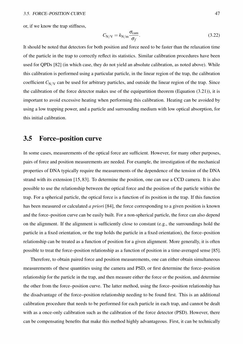
3.5. FORCE–POSITION CURVE 47
or, if we know the trap stiffness,
CN/V = kN/mσcam
σ f. (3.22)
It should be noted that detectors for both position and force need to be faster than the relaxation time
of the particle in the trap to correctly reflect its statistics. Similar calibration procedures have been
used for QPDs [82] (in which case, they do not yield an absolute calibration, as noted above). While
this calibration is performed using a particular particle, in the linear region of the trap, the calibration
coefficient CN/V can be used for arbitrary particles, and outside the linear region of the trap. Since
the calibration of the force detector makes use of the equipartition theorem (Equation (3.21)), it is
important to avoid excessive heating when performing this calibration. Heating can be avoided by
using a low trapping power, and a particle and surrounding medium with low optical absorption, for
this initial calibration.
3.5 Force–position curve
In some cases, measurements of the optical force are sufficient. However, for many other purposes,
pairs of force and position measurements are needed. For example, the investigation of the mechanical
properties of DNA typically require the measurements of the dependence of the tension of the DNA
strand with its extension [15, 83]. To determine the position, one can use a CCD camera. It is also
possible to use the relationship between the optical force and the position of the particle within the
trap. For a spherical particle, the optical force is a function of its position in the trap. If this function
has been measured or calculated a priori [84], the force corresponding to a given position is known
and the force–position curve can be easily built. For a non-spherical particle, the force can also depend
on the alignment. If the alignment is sufficiently close to constant (e.g., the surroundings hold the
particle in a fixed orientation, or the trap holds the particle in a fixed orientation), the force–position
relationship can be treated as a function of position for a given alignment. More generally, it is often
possible to treat the force–position relationship as a function of position in a time-averaged sense [85].
Therefore, to obtain paired force and position measurements, one can either obtain simultaneous
measurements of these quantities using the camera and PSD, or first determine the force–position
relationship for the particle in the trap, and then measure either the force or the position, and determine
the other from the force–position curve. The latter method, using the force–position relationship has
the disadvantage of the force–position relationship needing to be found first. This is an additional
calibration procedure that needs to be performed for each particle in each trap, and cannot be dealt
with as a once-only calibration such as the calibration of the force detector (PSD). However, there
can be compensating benefits that make this method highly advantageous. First, it can be technically
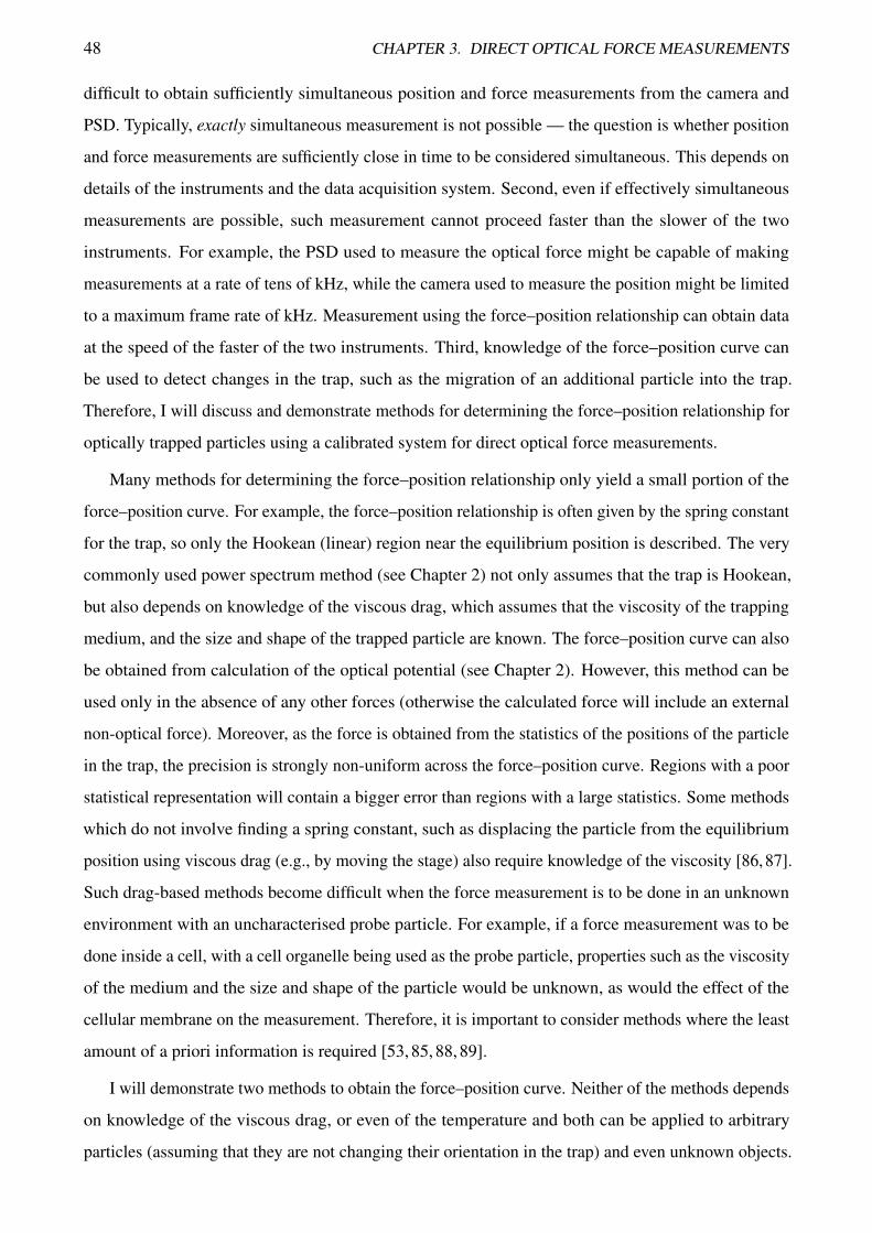
48 CHAPTER 3. DIRECT OPTICAL FORCE MEASUREMENTS
difficult to obtain sufficiently simultaneous position and force measurements from the camera and
PSD. Typically, exactly simultaneous measurement is not possible — the question is whether position
and force measurements are sufficiently close in time to be considered simultaneous. This depends on
details of the instruments and the data acquisition system. Second, even if effectively simultaneous
measurements are possible, such measurement cannot proceed faster than the slower of the two
instruments. For example, the PSD used to measure the optical force might be capable of making
measurements at a rate of tens of kHz, while the camera used to measure the position might be limited
to a maximum frame rate of kHz. Measurement using the force–position relationship can obtain data
at the speed of the faster of the two instruments. Third, knowledge of the force–position curve can
be used to detect changes in the trap, such as the migration of an additional particle into the trap.
Therefore, I will discuss and demonstrate methods for determining the force–position relationship for
optically trapped particles using a calibrated system for direct optical force measurements.
Many methods for determining the force–position relationship only yield a small portion of the
force–position curve. For example, the force–position relationship is often given by the spring constant
for the trap, so only the Hookean (linear) region near the equilibrium position is described. The very
commonly used power spectrum method (see Chapter 2) not only assumes that the trap is Hookean,
but also depends on knowledge of the viscous drag, which assumes that the viscosity of the trapping
medium, and the size and shape of the trapped particle are known. The force–position curve can also
be obtained from calculation of the optical potential (see Chapter 2). However, this method can be
used only in the absence of any other forces (otherwise the calculated force will include an external
non-optical force). Moreover, as the force is obtained from the statistics of the positions of the particle
in the trap, the precision is strongly non-uniform across the force–position curve. Regions with a poor
statistical representation will contain a bigger error than regions with a large statistics. Some methods
which do not involve finding a spring constant, such as displacing the particle from the equilibrium
position using viscous drag (e.g., by moving the stage) also require knowledge of the viscosity [86,87].
Such drag-based methods become difficult when the force measurement is to be done in an unknown
environment with an uncharacterised probe particle. For example, if a force measurement was to be
done inside a cell, with a cell organelle being used as the probe particle, properties such as the viscosity
of the medium and the size and shape of the particle would be unknown, as would the effect of the
cellular membrane on the measurement. Therefore, it is important to consider methods where the least
amount of a priori information is required [53, 85, 88, 89].
I will demonstrate two methods to obtain the force–position curve. Neither of the methods depends
on knowledge of the viscous drag, or even of the temperature and both can be applied to arbitrary
particles (assuming that they are not changing their orientation in the trap) and even unknown objects.
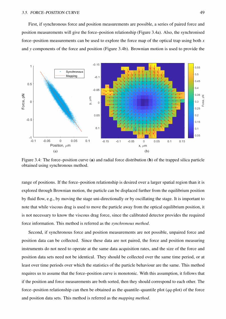
3.5. FORCE–POSITION CURVE 49
First, if synchronous force and position measurements are possible, a series of paired force and
position measurements will give the force–position relationship (Figure 3.4a). Also, the synchronised
force–position measurements can be used to explore the force map of the optical trap using both x
and y components of the force and position (Figure 3.4b). Brownian motion is used to provide the
(a) (b)
Figure 3.4: The force–position curve (a) and radial force distribution (b) of the trapped silica particleobtained using synchronous method.
range of positions. If the force–position relationship is desired over a larger spatial region than it is
explored through Brownian motion, the particle can be displaced further from the equilibrium position
by fluid flow, e.g., by moving the stage uni-directionally or by oscillating the stage. It is important to
note that while viscous drag is used to move the particle away from the optical equilibrium position, it
is not necessary to know the viscous drag force, since the calibrated detector provides the required
force information. This method is referred as the synchronous method.
Second, if synchronous force and position measurements are not possible, unpaired force and
position data can be collected. Since these data are not paired, the force and position measuring
instruments do not need to operate at the same data acquisition rates, and the size of the force and
position data sets need not be identical. They should be collected over the same time period, or at
least over time periods over which the statistics of the particle behaviour are the same. This method
requires us to assume that the force–position curve is monotonic. With this assumption, it follows that
if the position and force measurements are both sorted, then they should correspond to each other. The
force–position relationship can then be obtained as the quantile–quantile plot (qq-plot) of the force
and position data sets. This method is referred as the mapping method.
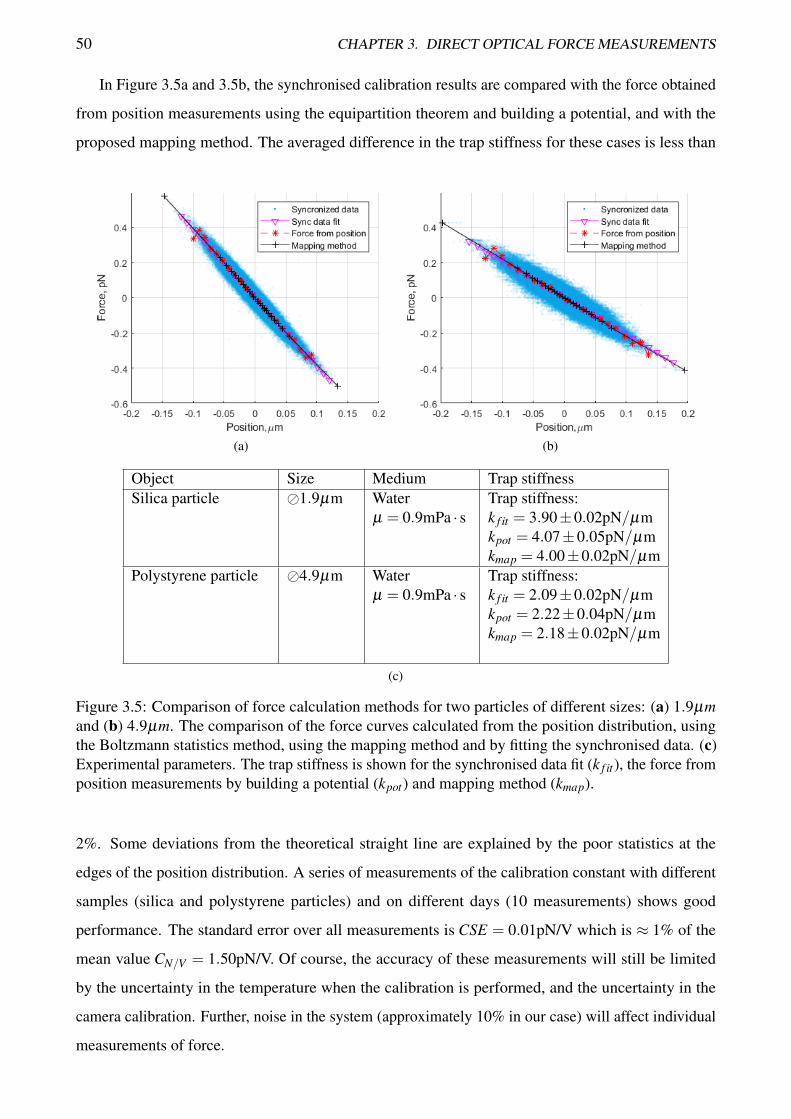
50 CHAPTER 3. DIRECT OPTICAL FORCE MEASUREMENTS
In Figure 3.5a and 3.5b, the synchronised calibration results are compared with the force obtained
from position measurements using the equipartition theorem and building a potential, and with the
proposed mapping method. The averaged difference in the trap stiffness for these cases is less than
(a) (b)
Object Size Medium Trap stiffnessSilica particle �1.9µm Water
µ = 0.9mPa · sTrap stiffness:k f it = 3.90±0.02pN/µmkpot = 4.07±0.05pN/µmkmap = 4.00±0.02pN/µm
Polystyrene particle �4.9µm Waterµ = 0.9mPa · s
Trap stiffness:k f it = 2.09±0.02pN/µmkpot = 2.22±0.04pN/µmkmap = 2.18±0.02pN/µm
(c)
Figure 3.5: Comparison of force calculation methods for two particles of different sizes: (a) 1.9µmand (b) 4.9µm. The comparison of the force curves calculated from the position distribution, usingthe Boltzmann statistics method, using the mapping method and by fitting the synchronised data. (c)Experimental parameters. The trap stiffness is shown for the synchronised data fit (k f it), the force fromposition measurements by building a potential (kpot) and mapping method (kmap).
2%. Some deviations from the theoretical straight line are explained by the poor statistics at the
edges of the position distribution. A series of measurements of the calibration constant with different
samples (silica and polystyrene particles) and on different days (10 measurements) shows good
performance. The standard error over all measurements is CSE = 0.01pN/V which is ≈ 1% of the
mean value CN/V = 1.50pN/V. Of course, the accuracy of these measurements will still be limited
by the uncertainty in the temperature when the calibration is performed, and the uncertainty in the
camera calibration. Further, noise in the system (approximately 10% in our case) will affect individual
measurements of force.
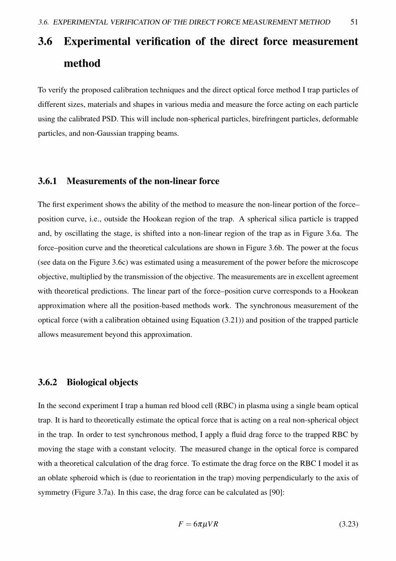
3.6. EXPERIMENTAL VERIFICATION OF THE DIRECT FORCE MEASUREMENT METHOD 51
3.6 Experimental verification of the direct force measurement
method
To verify the proposed calibration techniques and the direct optical force method I trap particles of
different sizes, materials and shapes in various media and measure the force acting on each particle
using the calibrated PSD. This will include non-spherical particles, birefringent particles, deformable
particles, and non-Gaussian trapping beams.
3.6.1 Measurements of the non-linear force
The first experiment shows the ability of the method to measure the non-linear portion of the force–
position curve, i.e., outside the Hookean region of the trap. A spherical silica particle is trapped
and, by oscillating the stage, is shifted into a non-linear region of the trap as in Figure 3.6a. The
force–position curve and the theoretical calculations are shown in Figure 3.6b. The power at the focus
(see data on the Figure 3.6c) was estimated using a measurement of the power before the microscope
objective, multiplied by the transmission of the objective. The measurements are in excellent agreement
with theoretical predictions. The linear part of the force–position curve corresponds to a Hookean
approximation where all the position-based methods work. The synchronous measurement of the
optical force (with a calibration obtained using Equation (3.21)) and position of the trapped particle
allows measurement beyond this approximation.
3.6.2 Biological objects
In the second experiment I trap a human red blood cell (RBC) in plasma using a single beam optical
trap. It is hard to theoretically estimate the optical force that is acting on a real non-spherical object
in the trap. In order to test synchronous method, I apply a fluid drag force to the trapped RBC by
moving the stage with a constant velocity. The measured change in the optical force is compared
with a theoretical calculation of the drag force. To estimate the drag force on the RBC I model it as
an oblate spheroid which is (due to reorientation in the trap) moving perpendicularly to the axis of
symmetry (Figure 3.7a). In this case, the drag force can be calculated as [90]:
F = 6πµV R (3.23)
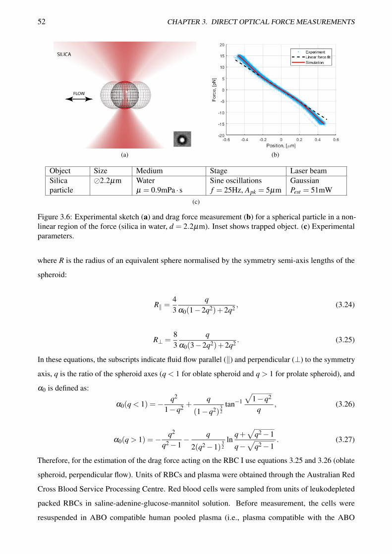
52 CHAPTER 3. DIRECT OPTICAL FORCE MEASUREMENTS
(a) (b)
Object Size Medium Stage Laser beamSilicaparticle
�2.2µm Waterµ = 0.9mPa · s
Sine oscillationsf = 25Hz, Apk = 5µm
GaussianPest = 51mW
(c)
Figure 3.6: Experimental sketch (a) and drag force measurement (b) for a spherical particle in a non-linear region of the force (silica in water, d = 2.2µm). Inset shows trapped object. (c) Experimentalparameters.
where R is the radius of an equivalent sphere normalised by the symmetry semi-axis lengths of the
spheroid:
R‖ =43
qα0(1−2q2)+2q2 , (3.24)
R⊥ =83
qα0(3−2q2)+2q2 . (3.25)
In these equations, the subscripts indicate fluid flow parallel (‖) and perpendicular (⊥) to the symmetry
axis, q is the ratio of the spheroid axes (q < 1 for oblate spheroid and q > 1 for prolate spheroid), and
α0 is defined as:
α0(q < 1) =− q2
1−q2 +q
(1−q2)32
tan−1
√1−q2
q, (3.26)
α0(q > 1) =− q2
q2−1− q
2(q2−1)32
lnq+√
q2−1
q−√
q2−1. (3.27)
Therefore, for the estimation of the drag force acting on the RBC I use equations 3.25 and 3.26 (oblate
spheroid, perpendicular flow). Units of RBCs and plasma were obtained through the Australian Red
Cross Blood Service Processing Centre. Red blood cells were sampled from units of leukodepleted
packed RBCs in saline-adenine-glucose-mannitol solution. Before measurement, the cells were
resuspended in ABO compatible human pooled plasma (i.e., plasma compatible with the ABO
3.6. EXPERIMENTAL VERIFICATION OF THE DIRECT FORCE MEASUREMENT METHOD 53
(a)
4 5 6 7 8 9 10 11 12 13
Drag force, pN
4
5
6
7
8
9
10
11
12
13
Optical fo
rce, pN
Fopt
=1.02Fdrag
-0.00055
Experiment
Linear fit
(b)
(c)
3 4 5 6 7 8 9 10 11 12
Drag force, pN
3
4
5
6
7
8
9
10
11
Optical fo
rce, pN
Fopt
=1.02Fdrag
-0.22
Experiment
Linear fit
(d)
Object Size Medium Stage Linear fitRMSE
RBC 5.0×�8.4µm Plasmaµ = 1.43mPa · s
v =[50,75,100,125]µm/s
0.11pN
‘Blob’(stretchable)
5.3×6.8µm,5.1×7.0µm,5.0×6.8µm,4.8×8.3µm,4.8×8.8µm
Plasmaµ = 1.43mPa · s
v =[50,75,100,125,150]µm/s
0.04pN
(e)
Figure 3.7: Experimental sketch (a) and result (b) for trapped RBC in Stokes flow. Fluid drag forceacting on the trapped RBC in plasma for different stage velocities. The drag force is that acting on anoblate spheroid of the same size (5.0×8.4µm ) as the RBC. Experimental sketch (c) and result (d) forthe trapped blob in Stokes flow. The inset images show the change in shape of the blob as the flowspeed changes. Modelled as a prolate spheroid with parameters corresponding to the measured size ofthe blob. Insets on the (a) and (c) show trapped object. (e) Experimental parameters.
blood type of the RBCs) to reproduce a physiological environment. The viscosity of the plasma is
µ = 1.43±0.08 cP [91].
Again, the current measurements of this RBC, shown in Figure 3.7b, are in close agreement with
the theoretical calculations. Thus, even a simplified model of the RBC can effectively describe its
54 CHAPTER 3. DIRECT OPTICAL FORCE MEASUREMENTS
behaviour.
Next, I show the viability of absolute calibration of an arbitrary particle by measuring the drag
force acting on an unknown particle which was found in the sample of RBCs, henceforth referred to as
the “blob”, shown in Figure 3.7c. Unlike the RBCs, the blob is roughly a prolate spheroid and does not
orientate itself in the trap as a RBC does. For the calculations of the drag force a model of a prolate
spheroid with a flow parallel to the symmetry axes (equations 3.24 and 3.27) is used. The measured
drag force and the theoretical calculations are shown in Figure 3.7d. As the blob’s walls are very soft,
we can see a stretching of this structure at high velocities (v > 125 µm/s). For these cases the blob is
stretching out of the region of observation. I measure the size of the blob by fitting an ellipse to the
visible part of the blob (which is > 90% of the length of the blob). However, even in this situation,
the results are in close agreement with the theoretical prediction when the change in the size is taken
into account. Thus, I was able to measure the optical force acting on a structure with a variable shape
which is extremely difficult to do with other methods.
3.6.3 Birefringent particles
Next, I show that the calibration is also correct for birefringent particles. A vaterite microsphere is
being trapped [92], and we apply a fluid drag force (Figure 3.8a). Since the vaterite particle aligns
with its optic axis in the direction of linear polarisation of the trap [93], I present results for drag
force applied in the direction of polarisation and normal to the direction of polarisation in Figure 3.8b
with all the parameters shown in Figure 3.8c. The lines comparing optical to drag forces for the two
directions are offset since I assume that the vaterite particle is spherical, and do not account for its
small asphericity.
3.6.4 Non-Gaussian beams
Finally, I demonstrate that the same calibration remains correct if the structure of trapping beam is
changed. Here, I use an HG10 beam to trap a polystyrene microsphere (Figure 3.9a). Since the focal
spot of an HG10 beam consists of two spots in one direction, I show the response for drag force applied
both in this direction and normal to it, in Figure 3.9b. The particle was chosen to be sufficiently large
to trap within both maxima to avoid hopping between them as this would make a comparison with
calculated drag force much more complicated.
The measured optical force is in good agreement with the calculated drag force for both directions.
The measurement of the force for such a non-Gaussian beam using position measurements will be
a much more complicated task. Firstly, it will require two calibrations for the two axes because of
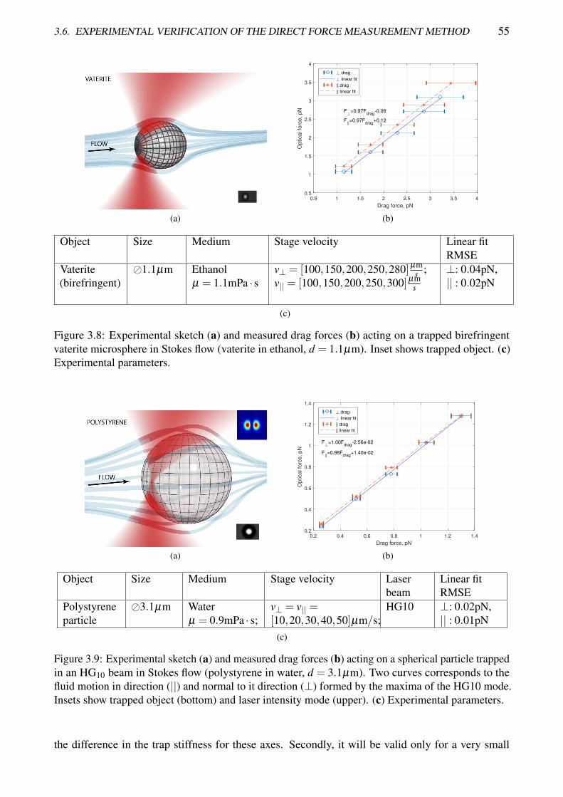
3.6. EXPERIMENTAL VERIFICATION OF THE DIRECT FORCE MEASUREMENT METHOD 55
(a)
0.5 1 1.5 2 2.5 3 3.5 4
Drag force, pN
0.5
1
1.5
2
2.5
3
3.5
4
Optical fo
rce, pN F =0.97F
drag-0.06
F||=0.97F
drag+0.12
drag
linear fit
|| drag
|| linear fit
(b)
Object Size Medium Stage velocity Linear fitRMSE
Vaterite(birefringent)
�1.1µm Ethanolµ = 1.1mPa · s
v⊥ = [100,150,200,250,280]µms ;
v|| = [100,150,200,250,300]µms
⊥: 0.04pN,|| : 0.02pN
(c)
Figure 3.8: Experimental sketch (a) and measured drag forces (b) acting on a trapped birefringentvaterite microsphere in Stokes flow (vaterite in ethanol, d = 1.1µm). Inset shows trapped object. (c)Experimental parameters.
(a)
0.2 0.4 0.6 0.8 1 1.2 1.4
Drag force, pN
0.2
0.4
0.6
0.8
1
1.2
1.4
Optical fo
rce, pN
F =1.00Fdrag
-2.56e-02
F||=0.98F
drag+1.40e-02
drag
linear fit
|| drag
|| linear fit
(b)
Object Size Medium Stage velocity Laserbeam
Linear fitRMSE
Polystyreneparticle
�3.1µm Waterµ = 0.9mPa · s;
v⊥ = v|| =[10,20,30,40,50]µm/s;
HG10 ⊥: 0.02pN,|| : 0.01pN
(c)
Figure 3.9: Experimental sketch (a) and measured drag forces (b) acting on a spherical particle trappedin an HG10 beam in Stokes flow (polystyrene in water, d = 3.1µm). Two curves corresponds to thefluid motion in direction (||) and normal to it direction (⊥) formed by the maxima of the HG10 mode.Insets show trapped object (bottom) and laser intensity mode (upper). (c) Experimental parameters.
the difference in the trap stiffness for these axes. Secondly, it will be valid only for a very small
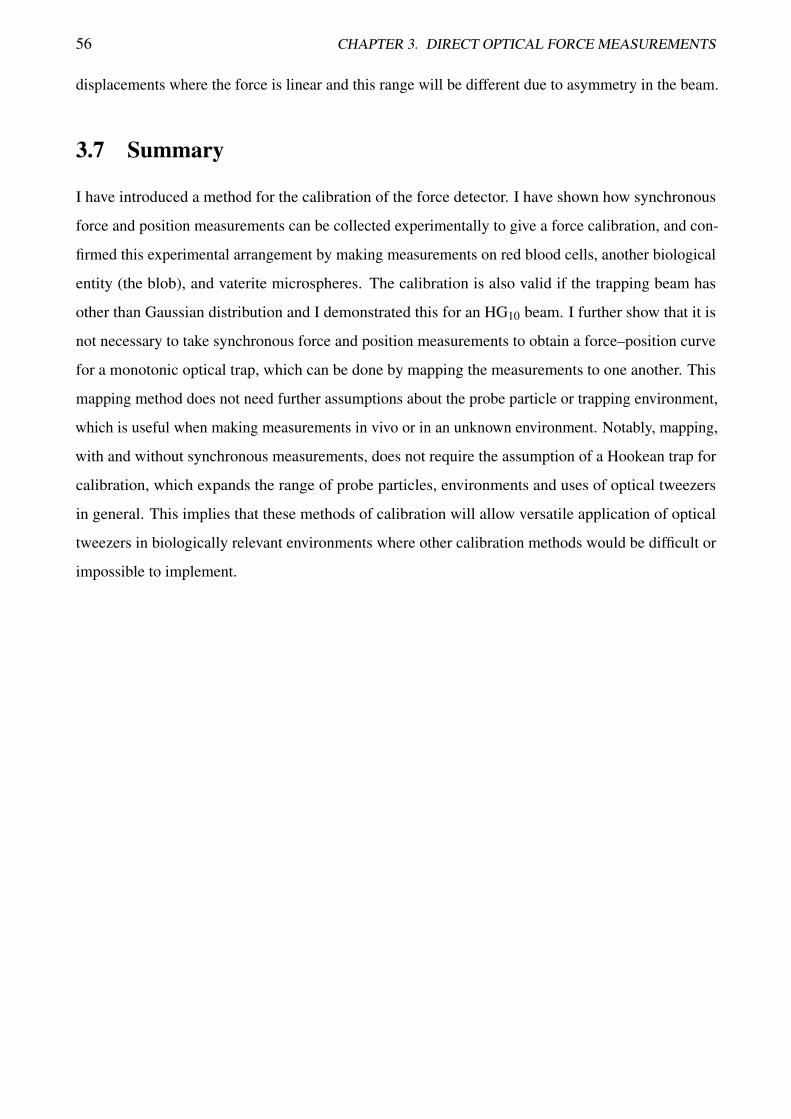
56 CHAPTER 3. DIRECT OPTICAL FORCE MEASUREMENTS
displacements where the force is linear and this range will be different due to asymmetry in the beam.
3.7 Summary
I have introduced a method for the calibration of the force detector. I have shown how synchronous
force and position measurements can be collected experimentally to give a force calibration, and con-
firmed this experimental arrangement by making measurements on red blood cells, another biological
entity (the blob), and vaterite microspheres. The calibration is also valid if the trapping beam has
other than Gaussian distribution and I demonstrated this for an HG10 beam. I further show that it is
not necessary to take synchronous force and position measurements to obtain a force–position curve
for a monotonic optical trap, which can be done by mapping the measurements to one another. This
mapping method does not need further assumptions about the probe particle or trapping environment,
which is useful when making measurements in vivo or in an unknown environment. Notably, mapping,
with and without synchronous measurements, does not require the assumption of a Hookean trap for
calibration, which expands the range of probe particles, environments and uses of optical tweezers
in general. This implies that these methods of calibration will allow versatile application of optical
tweezers in biologically relevant environments where other calibration methods would be difficult or
impossible to implement.

The following publication has been incorporated as Chapter 4.
1. A. V. Kashchuk, T. A. Nieminen, H. Rubinsztein-Dunlop, and A. B. Stilgoe. High-speed transverse
and axial optical force measurements using amplitude filter masks. Submitted to Scientific Reports.
Contributor Statement of contribution %A. V. Kashchuk conception and design 25
performed experiments 100analysis and interpretation 70preparation of text and figures 85
T. A. Nieminen conception and design 25analysis and interpretation 10supervision, guidance 30preparation of text and figures 5
H. Rubinsztein-Dunlop conception and design 25supervision, guidance 30analysis and interpretation 10preparation of text and figures 5
A. B. Stilgoe conception and design 25supervision, guidance 40analysis and interpretation 10preparation of text and figures 5

Chapter 4
Amplitude filter masks for 3-D optical force
measurements
Position sensitive detectors used for DFM are suitable only for radial force measurements (that is, a
PSD by itself). It is possible to get some information about the axial position by using an aperture [94];
however, this is a rather approximate estimation. 3-D forces can be calculated using a camera, as an
arbitrary function can be applied to the image. However, a camera has comparatively low bandwidth
and the frame rate for a full image typically will not exceed a few kilohertz. Also, there are millions
of pixels in a single camera chip, and therefore it has much higher noise than a single-element
photodetector. I propose a new detection method for performing a fast measurement of the optical
forces which at least matches the accuracy of the PSD, attains the high bandwidth and low noise of the
split detectors and gains the camera’s flexibility in the choice of the weighting functions.
4.1 Amplitude filter mask
The method for the high-speed transverse and axial force measurements is based upon a reflective filter
with a specific transmittance function which is placed in front of the photodetector to modulate the
intensity of the light transmitted through the optical system (Figure 4.1). A similar approach (but using
an attenuator with a spatially varying attenuation) was developed by Smith and Bustamante [95] for
measuring axial forces. In this method only a single detector is needed which implies that the method
is simpler to implement experimentally. In my method, the reflective mask allows the detection of both
transmitted and reflected beams as complementary information is contained in the two paths. This
doubles the signal and, unlike detection with the attenuator, preserves a uniform distribution of the
detection noise over the mask. Measuring both the reflected and transmitted light provides the optical59
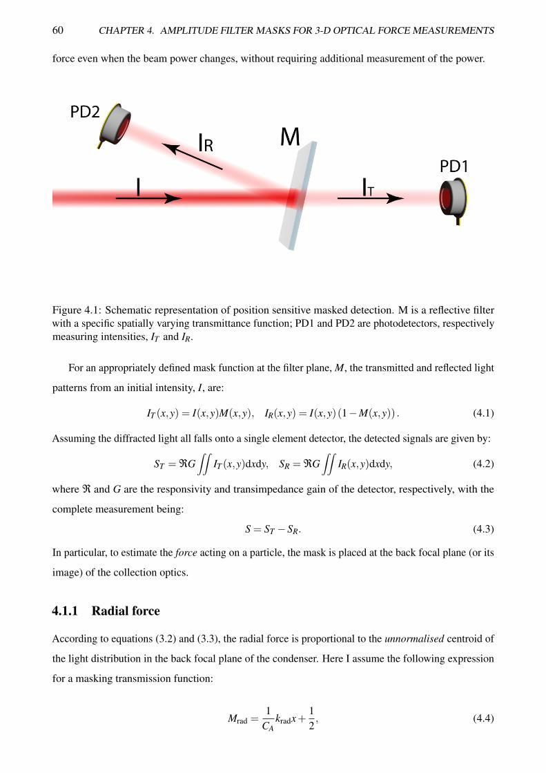
60 CHAPTER 4. AMPLITUDE FILTER MASKS FOR 3-D OPTICAL FORCE MEASUREMENTS
force even when the beam power changes, without requiring additional measurement of the power.
Figure 4.1: Schematic representation of position sensitive masked detection. M is a reflective filterwith a specific spatially varying transmittance function; PD1 and PD2 are photodetectors, respectivelymeasuring intensities, IT and IR.
For an appropriately defined mask function at the filter plane, M, the transmitted and reflected light
patterns from an initial intensity, I, are:
IT (x,y) = I(x,y)M(x,y), IR(x,y) = I(x,y)(1−M(x,y)) . (4.1)
Assuming the diffracted light all falls onto a single element detector, the detected signals are given by:
ST = ℜG∫∫
IT (x,y)dxdy, SR = ℜG∫∫
IR(x,y)dxdy, (4.2)
where ℜ and G are the responsivity and transimpedance gain of the detector, respectively, with the
complete measurement being:
S = ST −SR. (4.3)
In particular, to estimate the force acting on a particle, the mask is placed at the back focal plane (or its
image) of the collection optics.
4.1.1 Radial force
According to equations (3.2) and (3.3), the radial force is proportional to the unnormalised centroid of
the light distribution in the back focal plane of the condenser. Here I assume the following expression
for a masking transmission function:
Mrad =1
CAkradx+
12, (4.4)
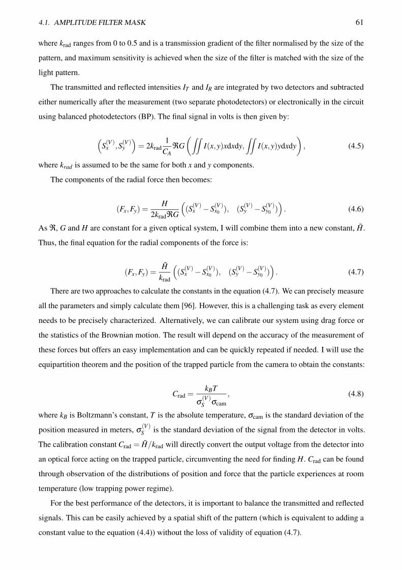
4.1. AMPLITUDE FILTER MASK 61
where krad ranges from 0 to 0.5 and is a transmission gradient of the filter normalised by the size of the
pattern, and maximum sensitivity is achieved when the size of the filter is matched with the size of the
light pattern.
The transmitted and reflected intensities IT and IR are integrated by two detectors and subtracted
either numerically after the measurement (two separate photodetectors) or electronically in the circuit
using balanced photodetectors (BP). The final signal in volts is then given by:
(S(V )
x ,S(V )y
)= 2krad
1CA
ℜG(∫∫
I(x,y)xdxdy,∫∫
I(x,y)ydxdy), (4.5)
where krad is assumed to be the same for both x and y components.
The components of the radial force then becomes:
(Fx,Fy) =H
2kradℜG
((S(V )
x −S(V )x0 ), (S(V )
y −S(V )y0 )). (4.6)
As ℜ, G and H are constant for a given optical system, I will combine them into a new constant, H.
Thus, the final equation for the radial components of the force is:
(Fx,Fy) =H
krad
((S(V )
x −S(V )x0 ), (S(V )
y −S(V )y0 )). (4.7)
There are two approaches to calculate the constants in the equation (4.7). We can precisely measure
all the parameters and simply calculate them [96]. However, this is a challenging task as every element
needs to be precisely characterized. Alternatively, we can calibrate our system using drag force or
the statistics of the Brownian motion. The result will depend on the accuracy of the measurement of
these forces but offers an easy implementation and can be quickly repeated if needed. I will use the
equipartition theorem and the position of the trapped particle from the camera to obtain the constants:
Crad =kBT
σ(V )S σcam
, (4.8)
where kB is Boltzmann’s constant, T is the absolute temperature, σcam is the standard deviation of the
position measured in meters, σ(V )S is the standard deviation of the signal from the detector in volts.
The calibration constant Crad = H/krad will directly convert the output voltage from the detector into
an optical force acting on the trapped particle, circumventing the need for finding H. Crad can be found
through observation of the distributions of position and force that the particle experiences at room
temperature (low trapping power regime).
For the best performance of the detectors, it is important to balance the transmitted and reflected
signals. This can be easily achieved by a spatial shift of the pattern (which is equivalent to adding a
constant value to the equation (4.4)) without the loss of validity of equation (4.7).
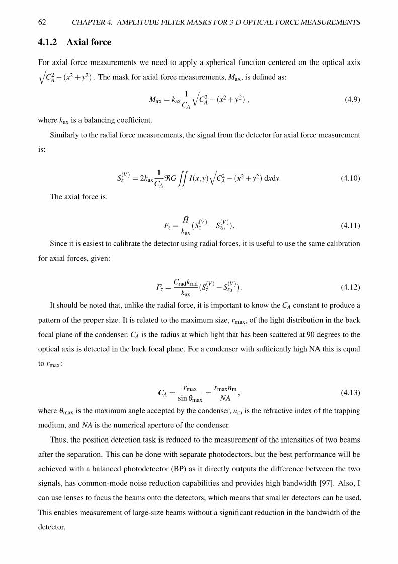
62 CHAPTER 4. AMPLITUDE FILTER MASKS FOR 3-D OPTICAL FORCE MEASUREMENTS
4.1.2 Axial force
For axial force measurements we need to apply a spherical function centered on the optical axis√C2
A− (x2 + y2) . The mask for axial force measurements, Max, is defined as:
Max = kax1
CA
√C2
A− (x2 + y2) , (4.9)
where kax is a balancing coefficient.
Similarly to the radial force measurements, the signal from the detector for axial force measurement
is:
S(V )z = 2kax
1CA
ℜG∫∫
I(x,y)√
C2A− (x2 + y2) dxdy. (4.10)
The axial force is:
Fz =Hkax
(S(V )z −S(V )
z0 ). (4.11)
Since it is easiest to calibrate the detector using radial forces, it is useful to use the same calibration
for axial forces, given:
Fz =Cradkrad
kax(S(V )
z −S(V )z0 ). (4.12)
It should be noted that, unlike the radial force, it is important to know the CA constant to produce a
pattern of the proper size. It is related to the maximum size, rmax, of the light distribution in the back
focal plane of the condenser. CA is the radius at which light that has been scattered at 90 degrees to the
optical axis is detected in the back focal plane. For a condenser with sufficiently high NA this is equal
to rmax:
CA =rmax
sinθmax=
rmaxnm
NA, (4.13)
where θmax is the maximum angle accepted by the condenser, nm is the refractive index of the trapping
medium, and NA is the numerical aperture of the condenser.
Thus, the position detection task is reduced to the measurement of the intensities of two beams
after the separation. This can be done with separate photodectors, but the best performance will be
achieved with a balanced photodetector (BP) as it directly outputs the difference between the two
signals, has common-mode noise reduction capabilities and provides high bandwidth [97]. Also, I
can use lenses to focus the beams onto the detectors, which means that smaller detectors can be used.
This enables measurement of large-size beams without a significant reduction in the bandwidth of the
detector.

4.2. DIGITAL MICROMIRROR DEVICE AS A DYNAMIC FILTER MASK 63
4.2 Digital micromirror device as a dynamic filter mask
A digital micromirror device or DMD is a micro-electrical-mechanical system which consists of an
array of micron-sized mirrors (typically, about one million mirrors) which are able to switch between
two stable positions [32, 98, 99]. Each mirror can be set to the “on” or “off” state individually. We can
use this property of the DMD to reflect the light into two different directions to perform the optical
force measurements. As a DMD is a binary modulator, I will use dithering [100] to represent different
transmission levels. Two types of patterns are being used: a linear gradient, equation (4.4), for radial
forces and a spherical gradient, equation (4.9), for axial force measurements. The linear gradient was
created with each line of the array (row or column) containing randomly distributed “on” pixels with
the number of pixels corresponding to the required transmission level. The spherical gradient was
created with the same algorithm but using circles instead of lines. Due to the pixelated structure of the
DMD, higher diffraction orders are present. However, as we perform a calibration of the detector, these
orders do not influence the measurements of the optical forces and can be filtered out with an aperture.
Figure 4.2: Digital micromirror device (DMD). Mirrors are flipping between two position: “on” (white)and “off” (purple).
4.2.1 Dithering
As a DMD is a binary modulator, we have to use dithering to represent a gradient on the pattern. The
accuracy of this representation depends on the ratio between the size of the individual mirror and the
size of the spot. I simulate the displacement of the Gaussian beam across the dithered pattern for
radial force measurement — linear gradient — and compare the results with the expected value (see
Figure 4.3a). The relative error drops quickly with an increase in the beam-to-pixel ratio (BPR is the
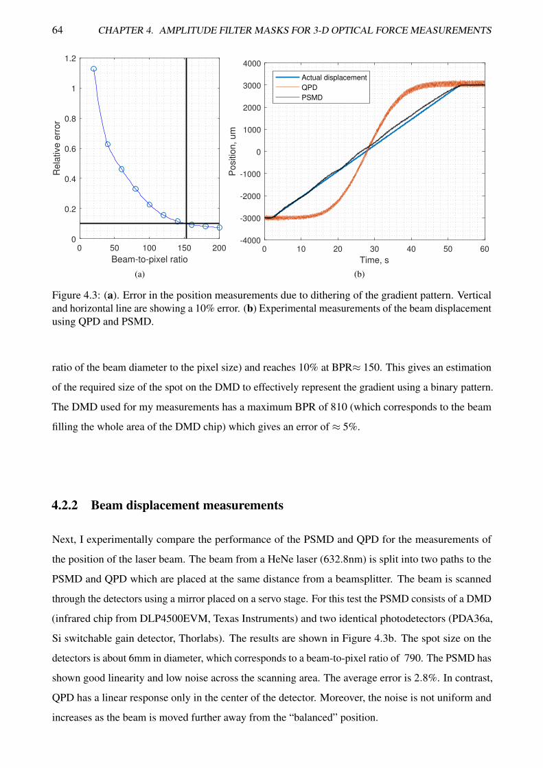
64 CHAPTER 4. AMPLITUDE FILTER MASKS FOR 3-D OPTICAL FORCE MEASUREMENTS
0 50 100 150 200
Beam-to-pixel ratio
0
0.2
0.4
0.6
0.8
1
1.2R
ela
tive
err
or
(a)
0 10 20 30 40 50 60
Time, s
-4000
-3000
-2000
-1000
0
1000
2000
3000
4000
Positio
n, um
Actual displacement
QPD
PSMD
(b)
Figure 4.3: (a). Error in the position measurements due to dithering of the gradient pattern. Verticaland horizontal line are showing a 10% error. (b) Experimental measurements of the beam displacementusing QPD and PSMD.
ratio of the beam diameter to the pixel size) and reaches 10% at BPR≈ 150. This gives an estimation
of the required size of the spot on the DMD to effectively represent the gradient using a binary pattern.
The DMD used for my measurements has a maximum BPR of 810 (which corresponds to the beam
filling the whole area of the DMD chip) which gives an error of ≈ 5%.
4.2.2 Beam displacement measurements
Next, I experimentally compare the performance of the PSMD and QPD for the measurements of
the position of the laser beam. The beam from a HeNe laser (632.8nm) is split into two paths to the
PSMD and QPD which are placed at the same distance from a beamsplitter. The beam is scanned
through the detectors using a mirror placed on a servo stage. For this test the PSMD consists of a DMD
(infrared chip from DLP4500EVM, Texas Instruments) and two identical photodetectors (PDA36a,
Si switchable gain detector, Thorlabs). The results are shown in Figure 4.3b. The spot size on the
detectors is about 6mm in diameter, which corresponds to a beam-to-pixel ratio of 790. The PSMD has
shown good linearity and low noise across the scanning area. The average error is 2.8%. In contrast,
QPD has a linear response only in the center of the detector. Moreover, the noise is not uniform and
increases as the beam is moved further away from the “balanced” position.
4.3. EXPERIMENTAL MEASUREMENTS WITH POSITION SENSITIVE MASKED DETECTION 65
4.3 Experimental measurements with position sensitive masked
detection
To investigate the performance of the proposed detection method the setup shown in Figure 4.4 was
constructed. Ytterbium doped fiber laser (YLR-10-1064-LP, 10W, 1064nm, IPG Photonics) is focused
by a high-NA objective (Olympus UPlanSApo 60×, water immersion, 1.2 NA) to create an optical
trap (see Figure 4.4). Light, scattered by a trapped object, is collected by a condenser (Olympus
UPlanSApo 100×, silicone oil immersion, 1.35 NA). The back focal plane of the condenser is imaged
on the force detectors using a telescope (lenses L1 and L2) and a beamsplitter BS. A CMOS camera is
used to track the position of the trapped particles. The detectors are: PSD (duo-lateral PSM2-10 with
OT-301DL amplifier, 15kHz, On-Trak Photonics); PSMD which includes DMD (infrared chip from
DLP4500EVM, Texas Instruments) and balanced photodetector (PDB210A/M, 1 MHz, Thorlabs).
The signal from the detectors is recorded using a data acquisition card (NI PCIe-6351, National
Instruments) and a custom made program in LabView (National Instruments).
The sample is made from two coverslips with double-sided adhesive tape as a spacer. This provides
an enclosed ≈ 100µm high sample chamber. The sample is held and moved by a 3-D piezo-stage (PI
P-563.3CD, Physik Instrumente).
Three experiments are performed using different configurations of our apparatus involving either
a PSD, PSMD or both devices. Firstly, I will show the high-bandwidth performance of the PSMD
method and compare it with the duo-lateral PSD. Secondly, I investigate the accuracy of the axial force
measurements and compare them with the Stokes drag force. Finally, by combining axial forces from
the PSMD with radial force measurements using the PSD, full 3-D force measurements on a spherical
particle adhered to a microscope coverslip are performed.
4.3.1 Alignment and calibration of the detectors
The CMOS camera was calibrated by moving and tracking a fixed spherical particle with a nanometer
precision piezo-stage. The calibration constant for all measurements is Ccam = 0.170±0.002µm/px.
The PSD was calibrated with a spherical silica particle with a diameter of 1.70µm. The position
of the particle (in meters) and the optical force (in volts) were recorded simultaneously at 5000fps
(camera) and 15kHz (PSD) respectively. Then, the calibration constant of the PSD was calculated
using equation (4.8) and has a value of CPSD = 1.93±0.02pN/V
PSMD alignment and calibration are done in a few steps (see Figure 4.5). Firstly, I align the pattern
on the DMD with the optical axis using horizontally/vertically divided patterns (an analogue of the
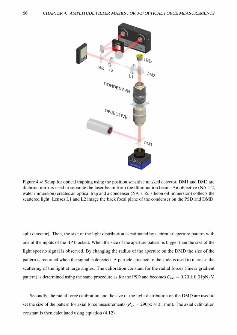
66 CHAPTER 4. AMPLITUDE FILTER MASKS FOR 3-D OPTICAL FORCE MEASUREMENTS
Figure 4.4: Setup for optical trapping using the position sensitive masked detector. DM1 and DM2 aredichroic mirrors used to separate the laser beam from the illumination beam. An objective (NA 1.2,water immersion) creates an optical trap and a condenser (NA 1.35, silicon oil immersion) collects thescattered light. Lenses L1 and L2 image the back focal plane of the condenser on the PSD and DMD.
split detector). Then, the size of the light distribution is estimated by a circular aperture pattern with
one of the inputs of the BP blocked. When the size of the aperture pattern is bigger than the size of the
light spot no signal is observed. By changing the radius of the aperture on the DMD the size of the
pattern is recorded when the signal is detected. A particle attached to the slide is used to increase the
scattering of the light at large angles. The calibration constant for the radial forces (linear gradient
pattern) is determined using the same procedure as for the PSD and becomes Crad = 0.70±0.01pN/V.
Secondly, the radial force calibration and the size of the light distribution on the DMD are used to
set the size of the pattern for axial force measurements (Rax = 290px≈ 3.1mm). The axial calibration
constant is then calculated using equation (4.12).
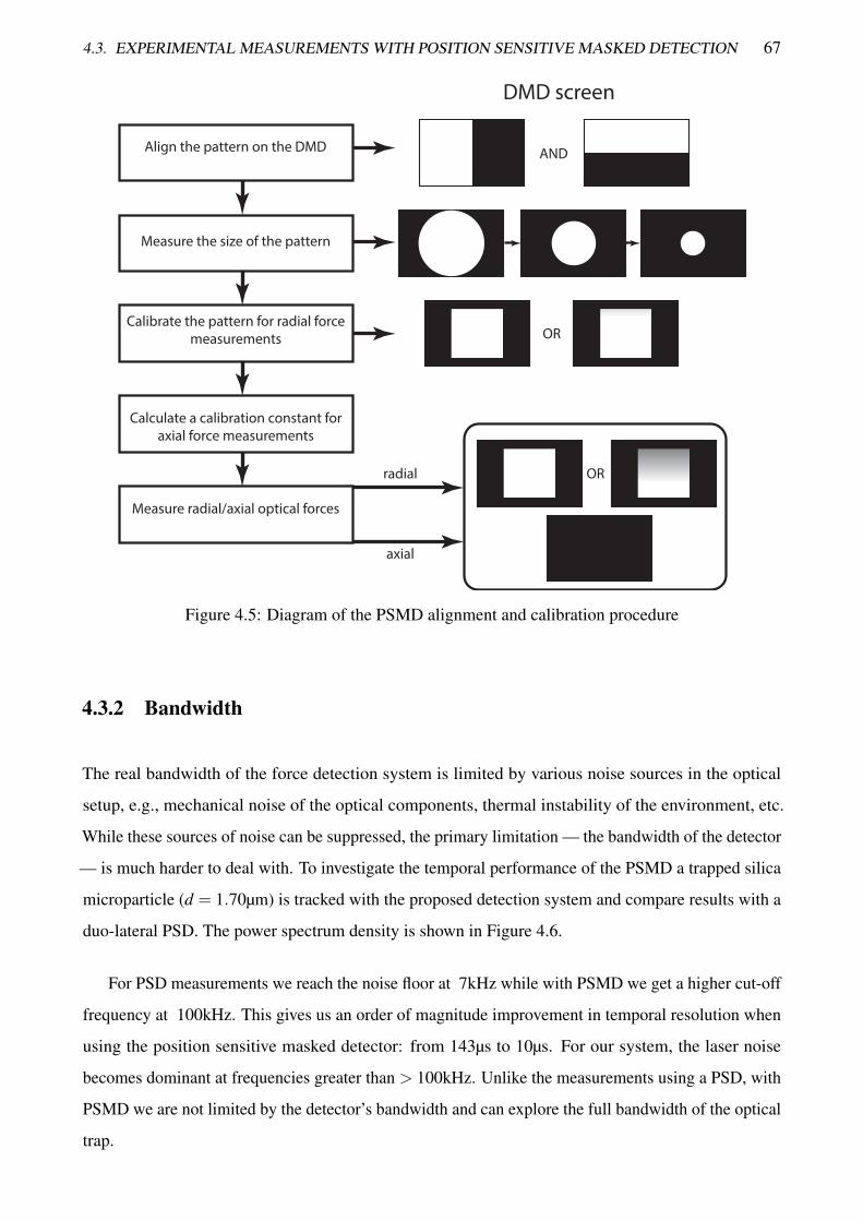
4.3. EXPERIMENTAL MEASUREMENTS WITH POSITION SENSITIVE MASKED DETECTION 67
Align the pattern on the DMD
DMD screen
Measure the size of the pattern
Calibrate the pattern for radial force
measurements
Calculate a calibration constant for
axial force measurements
Measure radial/axial optical forces
AND
OR
ORradial
axial
Figure 4.5: Diagram of the PSMD alignment and calibration procedure
4.3.2 Bandwidth
The real bandwidth of the force detection system is limited by various noise sources in the optical
setup, e.g., mechanical noise of the optical components, thermal instability of the environment, etc.
While these sources of noise can be suppressed, the primary limitation — the bandwidth of the detector
— is much harder to deal with. To investigate the temporal performance of the PSMD a trapped silica
microparticle (d = 1.70µm) is tracked with the proposed detection system and compare results with a
duo-lateral PSD. The power spectrum density is shown in Figure 4.6.
For PSD measurements we reach the noise floor at 7kHz while with PSMD we get a higher cut-off
frequency at 100kHz. This gives us an order of magnitude improvement in temporal resolution when
using the position sensitive masked detector: from 143µs to 10µs. For our system, the laser noise
becomes dominant at frequencies greater than > 100kHz. Unlike the measurements using a PSD, with
PSMD we are not limited by the detector’s bandwidth and can explore the full bandwidth of the optical
trap.
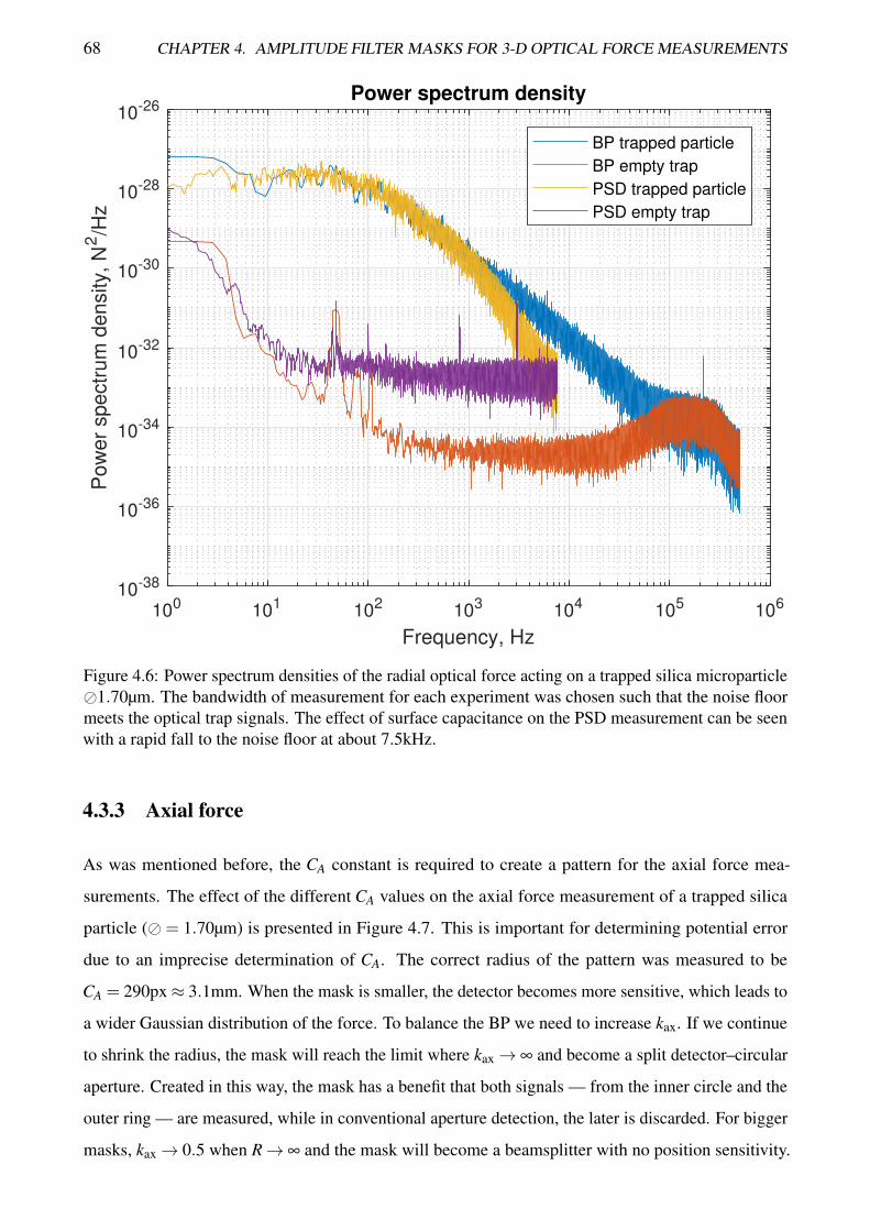
68 CHAPTER 4. AMPLITUDE FILTER MASKS FOR 3-D OPTICAL FORCE MEASUREMENTS
100 101 102 103 104 105 106
Frequency, Hz
10-38
10-36
10-34
10-32
10-30
10-28
10-26P
ow
er
sp
ectr
um
de
nsity,
N2/H
zPower spectrum density
BP trapped particle
BP empty trap
PSD trapped particle
PSD empty trap
Figure 4.6: Power spectrum densities of the radial optical force acting on a trapped silica microparticle�1.70µm. The bandwidth of measurement for each experiment was chosen such that the noise floormeets the optical trap signals. The effect of surface capacitance on the PSD measurement can be seenwith a rapid fall to the noise floor at about 7.5kHz.
4.3.3 Axial force
As was mentioned before, the CA constant is required to create a pattern for the axial force mea-
surements. The effect of the different CA values on the axial force measurement of a trapped silica
particle (� = 1.70µm) is presented in Figure 4.7. This is important for determining potential error
due to an imprecise determination of CA. The correct radius of the pattern was measured to be
CA = 290px≈ 3.1mm. When the mask is smaller, the detector becomes more sensitive, which leads to
a wider Gaussian distribution of the force. To balance the BP we need to increase kax. If we continue
to shrink the radius, the mask will reach the limit where kax→ ∞ and become a split detector–circular
aperture. Created in this way, the mask has a benefit that both signals — from the inner circle and the
outer ring — are measured, while in conventional aperture detection, the later is discarded. For bigger
masks, kax→ 0.5 when R→ ∞ and the mask will become a beamsplitter with no position sensitivity.
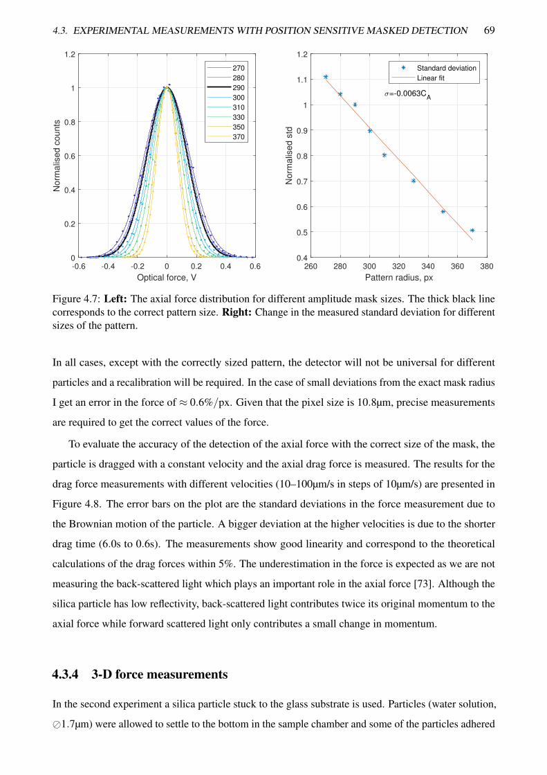
4.3. EXPERIMENTAL MEASUREMENTS WITH POSITION SENSITIVE MASKED DETECTION 69
-0.6 -0.4 -0.2 0 0.2 0.4 0.6
Optical force, V
0
0.2
0.4
0.6
0.8
1
1.2N
orm
alis
ed
co
un
ts
270
280
290
300
310
330
350
370
260 280 300 320 340 360 380
Pattern radius, px
0.4
0.5
0.6
0.7
0.8
0.9
1
1.1
1.2
No
rma
lise
d s
td
=-0.0063CA
Standard deviation
Linear fit
Figure 4.7: Left: The axial force distribution for different amplitude mask sizes. The thick black linecorresponds to the correct pattern size. Right: Change in the measured standard deviation for differentsizes of the pattern.
In all cases, except with the correctly sized pattern, the detector will not be universal for different
particles and a recalibration will be required. In the case of small deviations from the exact mask radius
I get an error in the force of ≈ 0.6%/px. Given that the pixel size is 10.8µm, precise measurements
are required to get the correct values of the force.
To evaluate the accuracy of the detection of the axial force with the correct size of the mask, the
particle is dragged with a constant velocity and the axial drag force is measured. The results for the
drag force measurements with different velocities (10–100µm/s in steps of 10µm/s) are presented in
Figure 4.8. The error bars on the plot are the standard deviations in the force measurement due to
the Brownian motion of the particle. A bigger deviation at the higher velocities is due to the shorter
drag time (6.0s to 0.6s). The measurements show good linearity and correspond to the theoretical
calculations of the drag forces within 5%. The underestimation in the force is expected as we are not
measuring the back-scattered light which plays an important role in the axial force [73]. Although the
silica particle has low reflectivity, back-scattered light contributes twice its original momentum to the
axial force while forward scattered light only contributes a small change in momentum.
4.3.4 3-D force measurements
In the second experiment a silica particle stuck to the glass substrate is used. Particles (water solution,
�1.7µm) were allowed to settle to the bottom in the sample chamber and some of the particles adhered
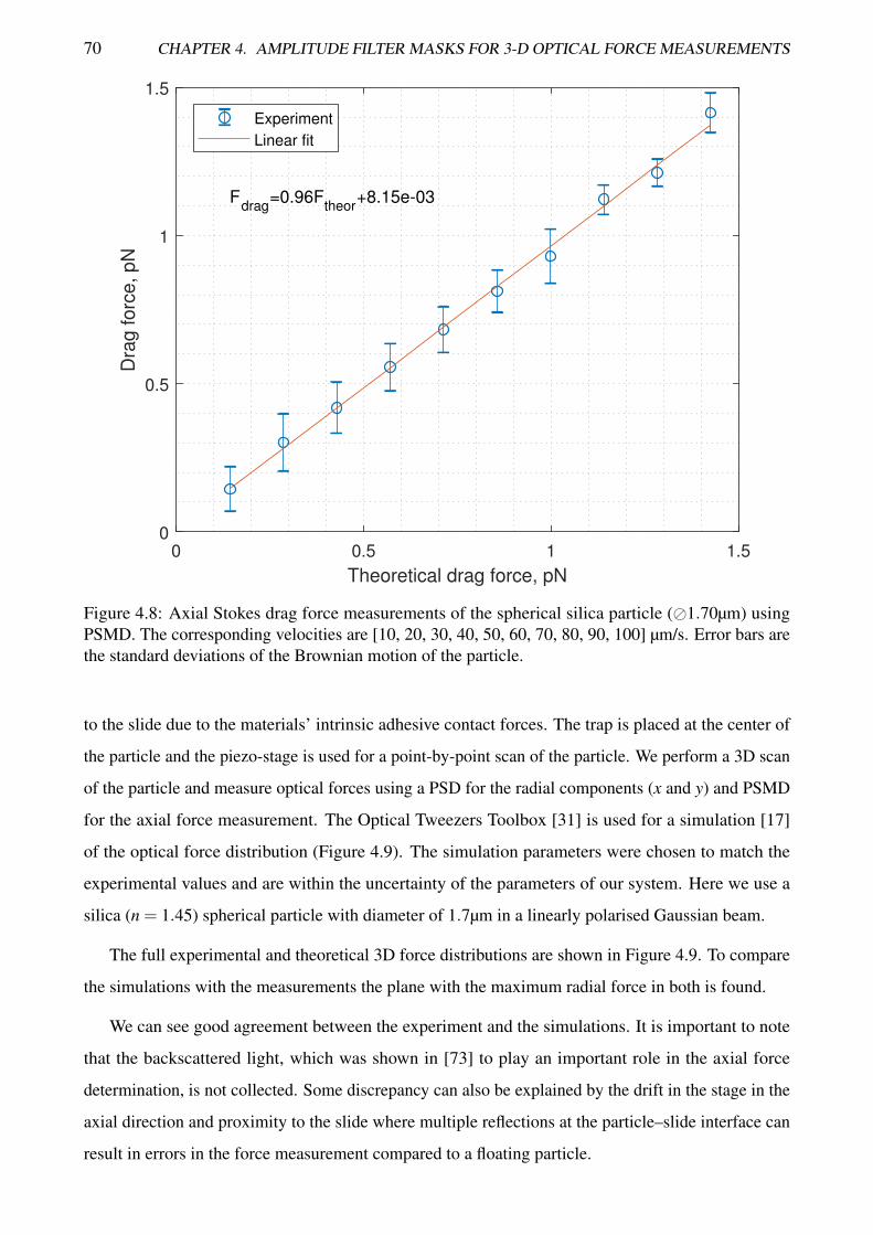
70 CHAPTER 4. AMPLITUDE FILTER MASKS FOR 3-D OPTICAL FORCE MEASUREMENTS
0 0.5 1 1.5
Theoretical drag force, pN
0
0.5
1
1.5
Dra
g forc
e, pN
Fdrag
=0.96Ftheor
+8.15e-03
Experiment
Linear fit
Figure 4.8: Axial Stokes drag force measurements of the spherical silica particle (�1.70µm) usingPSMD. The corresponding velocities are [10, 20, 30, 40, 50, 60, 70, 80, 90, 100] µm/s. Error bars arethe standard deviations of the Brownian motion of the particle.
to the slide due to the materials’ intrinsic adhesive contact forces. The trap is placed at the center of
the particle and the piezo-stage is used for a point-by-point scan of the particle. We perform a 3D scan
of the particle and measure optical forces using a PSD for the radial components (x and y) and PSMD
for the axial force measurement. The Optical Tweezers Toolbox [31] is used for a simulation [17]
of the optical force distribution (Figure 4.9). The simulation parameters were chosen to match the
experimental values and are within the uncertainty of the parameters of our system. Here we use a
silica (n = 1.45) spherical particle with diameter of 1.7µm in a linearly polarised Gaussian beam.
The full experimental and theoretical 3D force distributions are shown in Figure 4.9. To compare
the simulations with the measurements the plane with the maximum radial force in both is found.
We can see good agreement between the experiment and the simulations. It is important to note
that the backscattered light, which was shown in [73] to play an important role in the axial force
determination, is not collected. Some discrepancy can also be explained by the drift in the stage in the
axial direction and proximity to the slide where multiple reflections at the particle–slide interface can
result in errors in the force measurement compared to a floating particle.
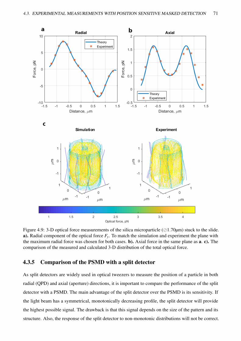
4.3. EXPERIMENTAL MEASUREMENTS WITH POSITION SENSITIVE MASKED DETECTION 71
Figure 4.9: 3-D optical force measurements of the silica microparticle (�1.70µm) stuck to the slide.a). Radial component of the optical force Fy. To match the simulation and experiment the plane withthe maximum radial force was chosen for both cases. b). Axial force in the same plane as a. c). Thecomparison of the measured and calculated 3-D distribution of the total optical force.
4.3.5 Comparison of the PSMD with a split detector
As split detectors are widely used in optical tweezers to measure the position of a particle in both
radial (QPD) and axial (aperture) directions, it is important to compare the performance of the split
detector with a PSMD. The main advantage of the split detector over the PSMD is its sensitivity. If
the light beam has a symmetrical, monotonically decreasing profile, the split detector will provide
the highest possible signal. The drawback is that this signal depends on the size of the pattern and its
structure. Also, the response of the split detector to non-monotonic distributions will not be correct.
72 CHAPTER 4. AMPLITUDE FILTER MASKS FOR 3-D OPTICAL FORCE MEASUREMENTS
This makes the usage of the split detectors for direct force measurements impossible as the universality
of the method will be lost.
4.4 Discussion and summary
I have shown that the PSMD has a much higher bandwidth compared to a typical PSD — resulting in
one order of magnitude increase in the bandwidth in our system (although, as was pointed out earlier,
higher bandwidth PSDs are available). In the experimental system, we are limited by the laser noise
but one can expect a much higher bandwidth (of the order of 10–100 MHz) if other sources of noise
are suppressed and a faster, low noise, photodetector is used. One of the factors that decreases the
bandwidth of the PSD is the size of the chip which determines the capacitance of the sensor which
in turn limits the response time of the detector. In PSMD the beam is separated by the amplitude
mask and this problem can be addressed by focusing the split beam onto a photodetector, so that the
smallest detectors can be used without loss in the resolution and linearity. Also, both the PSD and BP
in our system are silicon based detectors and have a low sensitivity at 1064nm. This may introduce an
additional low-pass filtering of the recorded signal [61].
A linear gradient pattern is used for the radial force measurement and provides a signal equivalent
to that of the PSD, as shown in Figure 4.6, where the power spectrum densities for both the PSD and
BP are the same for frequencies below 100 kHz. The linearity of the filter means that the detection is
proportional to the force and once calibrated should in principle always measure the radial (transverse)
optical force for a wide range of particles, both spherical and non-spherical.
The accuracy of the PSMD for the axial optical forces is estimated using the measurement of the
Stokes drag force on a sphere. The results show excellent linearity for the different velocities and very
little spread in the measurements demonstrating repeatability. However, the size of the pattern plays
a crucial role and the deviation of the radius of the pattern of just 10% will cause a 19% error in the
force measurement. Accurate calibration of the pattern is thus essential. However, this limitation is
imposed by the optical system and any method that measures the axial optical force will encounter this
same problem.
The theory behind the split detectors shows that they are the special cases of the masks for the
radial (QPD) and axial (aperture) force measurements with infinite slope of the gradient. This leads
to an increase in the sensitivity to the displacement at the cost of losing linearity. Therefore, split
detectors cannot be used for the direct optical force measurement, but remain valuable for position
measurement.
While the position sensitive masked detector can be implemented with a stationary filter, the use

4.4. DISCUSSION AND SUMMARY 73
of the DMD is preferable and has many advantages for the usability of the system. It allows the
implementation and testing of different patterns under the same conditions; characterisation of the
light distribution in the detector’s plane; convenient electronic alignment of the detector.
3-D forces can be measured using a combination of the detectors (Figure 4.9) or by time-sharing
the patterns on a single DMD. However, in the later case, the bandwidth of the measurements will be
limited by the framerate of the DMD, so the actual 3-D force measurement bandwidth will not exceed
a few kilohertz which is comparable with the bandwidth achievable with a camera.
The proposed method of measuring optical forces using amplitude filter masks (PSMD) expands
the universal direct force measurement method to a high bandwidth region which is inaccessible
with existing detectors. Moreover, it can improve the accuracy of force detection by accounting for
the variations in the transmission of the condenser for different angles and aberrations in the optical
system.

Chapter 5
Force measurements in biological systems
Mechanical forces play a vital role in any biological system. Measurement of these forces is crucial in
understanding the functionality and structural organisation of cells and tissues. On a single-cell level
these forces define the ability of the cell to maintain its shape and respond to external stresses. On a
multi-cell level mechanical forces establish an interaction between the cells and therefore determine
the structure of cell tissues. Many microscopic biological entities generate force to move themselves.
These include various swimming bacteria and sperms that use flagella to create a propulsion force.
The measurement of the propulsion force generated by these swimmers is important for understanding
the functionality of flagella and molecular motors involved in the motion.
Since the invention of optical trapping, biological systems have been some of the most interesting
targets of optical tweezers. Optical tweezers have a number of excellent properties which contribute to
its success with biosystems. The ability to apply and measure optical forces in the range of piconewtons,
which is inaccessible or hardly achievable with other techniques, has led to a huge number of biological
experiments using optical tweezers. They have been used for manipulation of organelles [101,102],
stretching of deoxyribonucleic acids (DNAs) [43, 103, 104], trapping of red blood cells (RBCs) [105]
(including trapping inside a living animal [106]), investigation of the cell membranes [107–109],
cytoskeletal networks [110], molecular motors [111, 112], and various in vivo experiments [113] in
biological objects.
In this chapter, I will present experimental results on the optical trapping and force measurements
of RBCs, including a study of the change in the stiffness of RBCs during cold storage. I will show
how a combination of position sensitive masked detector (PSMD; for axial force measurements) and
duo-lateral position sensitive detector (PSD; for radial force measurements) can be used to study the
motility of swimmers by measuring the propulsion force generated by a swimming Escherichia coli
(E. coli) bacterium.75
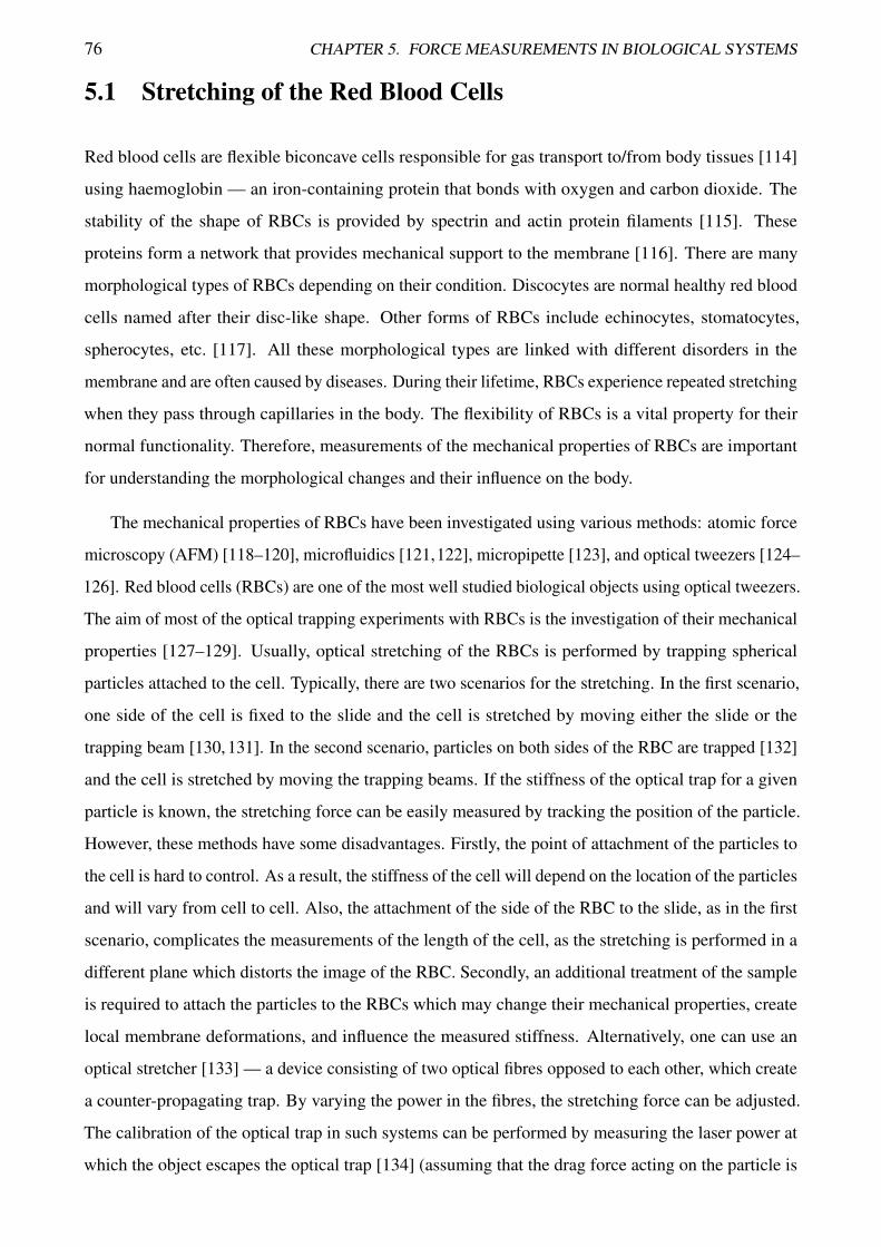
76 CHAPTER 5. FORCE MEASUREMENTS IN BIOLOGICAL SYSTEMS
5.1 Stretching of the Red Blood Cells
Red blood cells are flexible biconcave cells responsible for gas transport to/from body tissues [114]
using haemoglobin — an iron-containing protein that bonds with oxygen and carbon dioxide. The
stability of the shape of RBCs is provided by spectrin and actin protein filaments [115]. These
proteins form a network that provides mechanical support to the membrane [116]. There are many
morphological types of RBCs depending on their condition. Discocytes are normal healthy red blood
cells named after their disc-like shape. Other forms of RBCs include echinocytes, stomatocytes,
spherocytes, etc. [117]. All these morphological types are linked with different disorders in the
membrane and are often caused by diseases. During their lifetime, RBCs experience repeated stretching
when they pass through capillaries in the body. The flexibility of RBCs is a vital property for their
normal functionality. Therefore, measurements of the mechanical properties of RBCs are important
for understanding the morphological changes and their influence on the body.
The mechanical properties of RBCs have been investigated using various methods: atomic force
microscopy (AFM) [118–120], microfluidics [121,122], micropipette [123], and optical tweezers [124–
126]. Red blood cells (RBCs) are one of the most well studied biological objects using optical tweezers.
The aim of most of the optical trapping experiments with RBCs is the investigation of their mechanical
properties [127–129]. Usually, optical stretching of the RBCs is performed by trapping spherical
particles attached to the cell. Typically, there are two scenarios for the stretching. In the first scenario,
one side of the cell is fixed to the slide and the cell is stretched by moving either the slide or the
trapping beam [130, 131]. In the second scenario, particles on both sides of the RBC are trapped [132]
and the cell is stretched by moving the trapping beams. If the stiffness of the optical trap for a given
particle is known, the stretching force can be easily measured by tracking the position of the particle.
However, these methods have some disadvantages. Firstly, the point of attachment of the particles to
the cell is hard to control. As a result, the stiffness of the cell will depend on the location of the particles
and will vary from cell to cell. Also, the attachment of the side of the RBC to the slide, as in the first
scenario, complicates the measurements of the length of the cell, as the stretching is performed in a
different plane which distorts the image of the RBC. Secondly, an additional treatment of the sample
is required to attach the particles to the RBCs which may change their mechanical properties, create
local membrane deformations, and influence the measured stiffness. Alternatively, one can use an
optical stretcher [133] — a device consisting of two optical fibres opposed to each other, which create
a counter-propagating trap. By varying the power in the fibres, the stretching force can be adjusted.
The calibration of the optical trap in such systems can be performed by measuring the laser power at
which the object escapes the optical trap [134] (assuming that the drag force acting on the particle is
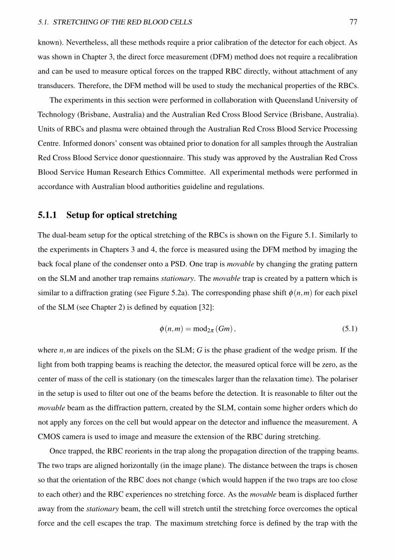
5.1. STRETCHING OF THE RED BLOOD CELLS 77
known). Nevertheless, all these methods require a prior calibration of the detector for each object. As
was shown in Chapter 3, the direct force measurement (DFM) method does not require a recalibration
and can be used to measure optical forces on the trapped RBC directly, without attachment of any
transducers. Therefore, the DFM method will be used to study the mechanical properties of the RBCs.
The experiments in this section were performed in collaboration with Queensland University of
Technology (Brisbane, Australia) and the Australian Red Cross Blood Service (Brisbane, Australia).
Units of RBCs and plasma were obtained through the Australian Red Cross Blood Service Processing
Centre. Informed donors’ consent was obtained prior to donation for all samples through the Australian
Red Cross Blood Service donor questionnaire. This study was approved by the Australian Red Cross
Blood Service Human Research Ethics Committee. All experimental methods were performed in
accordance with Australian blood authorities guideline and regulations.
5.1.1 Setup for optical stretching
The dual-beam setup for the optical stretching of the RBCs is shown on the Figure 5.1. Similarly to
the experiments in Chapters 3 and 4, the force is measured using the DFM method by imaging the
back focal plane of the condenser onto a PSD. One trap is movable by changing the grating pattern
on the SLM and another trap remains stationary. The movable trap is created by a pattern which is
similar to a diffraction grating (see Figure 5.2a). The corresponding phase shift φ(n,m) for each pixel
of the SLM (see Chapter 2) is defined by equation [32]:
φ(n,m) = mod2π (Gm) , (5.1)
where n,m are indices of the pixels on the SLM; G is the phase gradient of the wedge prism. If the
light from both trapping beams is reaching the detector, the measured optical force will be zero, as the
center of mass of the cell is stationary (on the timescales larger than the relaxation time). The polariser
in the setup is used to filter out one of the beams before the detection. It is reasonable to filter out the
movable beam as the diffraction pattern, created by the SLM, contain some higher orders which do
not apply any forces on the cell but would appear on the detector and influence the measurement. A
CMOS camera is used to image and measure the extension of the RBC during stretching.
Once trapped, the RBC reorients in the trap along the propagation direction of the trapping beams.
The two traps are aligned horizontally (in the image plane). The distance between the traps is chosen
so that the orientation of the RBC does not change (which would happen if the two traps are too close
to each other) and the RBC experiences no stretching force. As the movable beam is displaced further
away from the stationary beam, the cell will stretch until the stretching force overcomes the optical
force and the cell escapes the trap. The maximum stretching force is defined by the trap with the
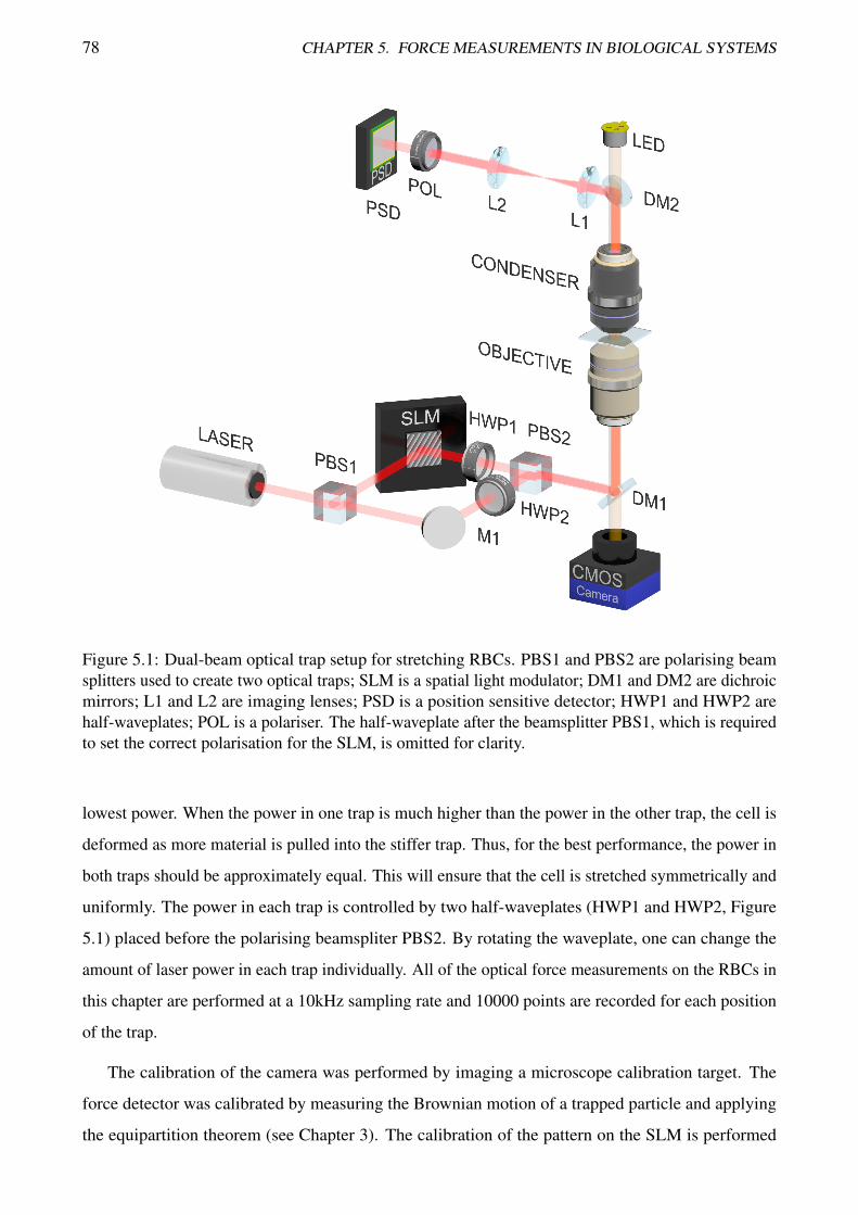
78 CHAPTER 5. FORCE MEASUREMENTS IN BIOLOGICAL SYSTEMS
Figure 5.1: Dual-beam optical trap setup for stretching RBCs. PBS1 and PBS2 are polarising beamsplitters used to create two optical traps; SLM is a spatial light modulator; DM1 and DM2 are dichroicmirrors; L1 and L2 are imaging lenses; PSD is a position sensitive detector; HWP1 and HWP2 arehalf-waveplates; POL is a polariser. The half-waveplate after the beamsplitter PBS1, which is requiredto set the correct polarisation for the SLM, is omitted for clarity.
lowest power. When the power in one trap is much higher than the power in the other trap, the cell is
deformed as more material is pulled into the stiffer trap. Thus, for the best performance, the power in
both traps should be approximately equal. This will ensure that the cell is stretched symmetrically and
uniformly. The power in each trap is controlled by two half-waveplates (HWP1 and HWP2, Figure
5.1) placed before the polarising beamspliter PBS2. By rotating the waveplate, one can change the
amount of laser power in each trap individually. All of the optical force measurements on the RBCs in
this chapter are performed at a 10kHz sampling rate and 10000 points are recorded for each position
of the trap.
The calibration of the camera was performed by imaging a microscope calibration target. The
force detector was calibrated by measuring the Brownian motion of a trapped particle and applying
the equipartition theorem (see Chapter 3). The calibration of the pattern on the SLM is performed
5.1. STRETCHING OF THE RED BLOOD CELLS 79
(a) (b)
Figure 5.2: (a) The grating pattern on the SLM. The grating gradient controls the position of the trap.(b) Calibration of the displacement of the movable trap by measuring the distance between two trappedparticles (silica, d = 1.68µm).
to determine the step in the displacement of the movable optical trap. Two spherical silica particles
(d = 1.68µm) were placed in the traps (one particle per trap) and tracked with a camera. The
corresponding distance between the particles was determined for a series of grating patterns (see Figure
5.2b). The measured displacement of the movable trap is measured as 0.16µm per integer increase of
spatial frequency across the SLM.
Determination of the length of the RBC in the trapping experiment is a challenging task as the
cell reorients in the trap along the beam propagation direction. As mentioned in the earlier part of
this chapter, the red blood cells are present in a large variety of shapes (discocytes, echinocytes,
stomatocytes, etc.) [117]. As the cell is stretched in the optical trap, the thickness and position of the
cell are also changed. This, in turn, changes the apparent brightness of the cell. Moreover, possible
variations in the background due to change in the illumination conditions (for example, due to diffusion
of other cells below the viewing plane or day-to-day changes in the illumination) also influence the
effectiveness of the detection of the RBCs. Therefore, it is hard to develop a universal algorithm which
accurately measures the size of RBCs. I devised a simple method to achieve consistent measurements
of the size of the RBCs using features of our optical system and known parameters of the image
capturing system (see Figure 5.3). Firstly, the averaged grayscale value of the background is subtracted
from the image, increasing the contrast of the cell. All the negative values (from the dark shadow
around the cell) are taken as positive grayscale values to account for parts of the cell below and
above the imaging plane. Secondly, as the trapping beams are aligned horizontally (relative to the
camera sensor), all the rows of the image are averaged. This gives a noticeable signal (blue line on the
Figure 5.3) which marks the horizontal edges of the cell. While it is possible to find the size of the cell
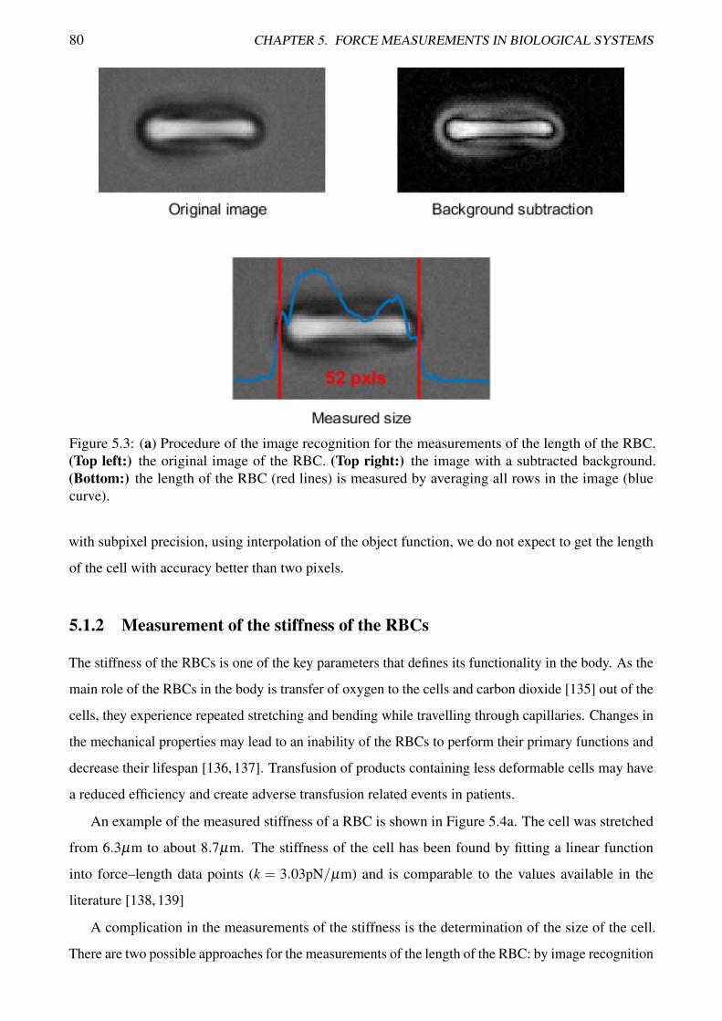
80 CHAPTER 5. FORCE MEASUREMENTS IN BIOLOGICAL SYSTEMS
Figure 5.3: (a) Procedure of the image recognition for the measurements of the length of the RBC.(Top left:) the original image of the RBC. (Top right:) the image with a subtracted background.(Bottom:) the length of the RBC (red lines) is measured by averaging all rows in the image (bluecurve).
with subpixel precision, using interpolation of the object function, we do not expect to get the length
of the cell with accuracy better than two pixels.
5.1.2 Measurement of the stiffness of the RBCs
The stiffness of the RBCs is one of the key parameters that defines its functionality in the body. As the
main role of the RBCs in the body is transfer of oxygen to the cells and carbon dioxide [135] out of the
cells, they experience repeated stretching and bending while travelling through capillaries. Changes in
the mechanical properties may lead to an inability of the RBCs to perform their primary functions and
decrease their lifespan [136, 137]. Transfusion of products containing less deformable cells may have
a reduced efficiency and create adverse transfusion related events in patients.
An example of the measured stiffness of a RBC is shown in Figure 5.4a. The cell was stretched
from 6.3µm to about 8.7µm. The stiffness of the cell has been found by fitting a linear function
into force–length data points (k = 3.03pN/µm) and is comparable to the values available in the
literature [138, 139]
A complication in the measurements of the stiffness is the determination of the size of the cell.
There are two possible approaches for the measurements of the length of the RBC: by image recognition
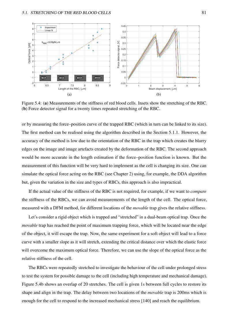
5.1. STRETCHING OF THE RED BLOOD CELLS 81
6 6.5 7 7.5 8 8.5 9
Length of the RBC, [ m]
-2
-1
0
1
2
3
4
5
6
7
8
9
Op
tica
l fo
rce
, [p
N] k
RBC=3.03pN/ m
Experiment
Linear fit
(a)
0 1 2 3 4 5 6
Beam displacement, [ m]
-0.05
0
0.05
0.1
0.15
0.2
0.25
0.3
0.35
0.4
0.45
Fo
rce
de
tecto
r sig
na
l, [
V]
(b)
Figure 5.4: (a) Measurements of the stiffness of red blood cells. Insets show the stretching of the RBC.(b) Force detector signal for a twenty times repeated stretching of the RBC.
or by measuring the force–position curve of the trapped RBC (which in turn can be linked to its size).
The first method can be realised using the algorithm described in the Section 5.1.1. However, the
accuracy of the method is low due to the orientation of the RBC in the trap which creates the blurry
edges on the image and image artefacts created by the deformation of the RBC. The second approach
would be more accurate in the length estimation if the force–position function is known. But the
measurement of this function will be very hard to implement as the cell is changing its size. One can
simulate the optical force acting on the RBC (see Chapter 2) using, for example, the DDA algorithm
but, given the variation in the size and types of RBCs, this approach is also impractical.
If the actual value of the stiffness of the RBC is not required, for example, if we want to compare
the stiffness of the RBCs, we can avoid measurements of the length of the cell. The optical force,
measured with a DFM method, for different locations of the movable trap gives the relative stiffness.
Let’s consider a rigid object which is trapped and “stretched” in a dual-beam optical trap. Once the
movable trap has reached the point of maximum trapping force, which will be located near the edge
of the object, it will escape the trap. Now, the same experiment for a soft object will lead to a force
curve with a smaller slope as it will stretch, extending the critical distance over which the elastic force
will overcome the maximum optical force. Therefore, we can use the slope of the optical force as the
relative stiffness of the cell.
The RBCs were repeatedly stretched to investigate the behaviour of the cell under prolonged stress
to test the system for possible damage to the cell (including high temperature and mechanical damage).
Figure 5.4b shows an overlap of 20 stretches. The cell is given 1s between full cycles to restore its
shape and align in the trap. The delay between two locations of the movable trap is 200ms which is
enough for the cell to respond to the increased mechanical stress [140] and reach the equilibrium.
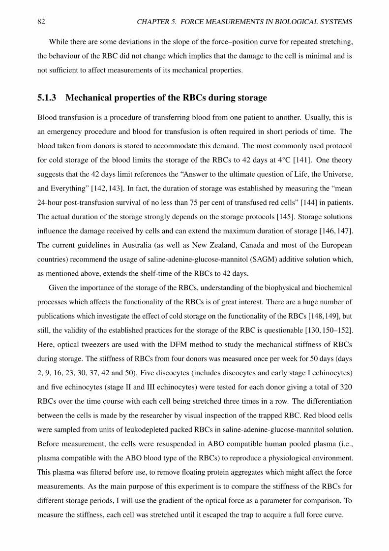
82 CHAPTER 5. FORCE MEASUREMENTS IN BIOLOGICAL SYSTEMS
While there are some deviations in the slope of the force–position curve for repeated stretching,
the behaviour of the RBC did not change which implies that the damage to the cell is minimal and is
not sufficient to affect measurements of its mechanical properties.
5.1.3 Mechanical properties of the RBCs during storage
Blood transfusion is a procedure of transferring blood from one patient to another. Usually, this is
an emergency procedure and blood for transfusion is often required in short periods of time. The
blood taken from donors is stored to accommodate this demand. The most commonly used protocol
for cold storage of the blood limits the storage of the RBCs to 42 days at 4°C [141]. One theory
suggests that the 42 days limit references the “Answer to the ultimate question of Life, the Universe,
and Everything” [142, 143]. In fact, the duration of storage was established by measuring the “mean
24-hour post-transfusion survival of no less than 75 per cent of transfused red cells” [144] in patients.
The actual duration of the storage strongly depends on the storage protocols [145]. Storage solutions
influence the damage received by cells and can extend the maximum duration of storage [146, 147].
The current guidelines in Australia (as well as New Zealand, Canada and most of the European
countries) recommend the usage of saline-adenine-glucose-mannitol (SAGM) additive solution which,
as mentioned above, extends the shelf-time of the RBCs to 42 days.
Given the importance of the storage of the RBCs, understanding of the biophysical and biochemical
processes which affects the functionality of the RBCs is of great interest. There are a huge number of
publications which investigate the effect of cold storage on the functionality of the RBCs [148,149], but
still, the validity of the established practices for the storage of the RBC is questionable [130, 150–152].
Here, optical tweezers are used with the DFM method to study the mechanical stiffness of RBCs
during storage. The stiffness of RBCs from four donors was measured once per week for 50 days (days
2, 9, 16, 23, 30, 37, 42 and 50). Five discocytes (includes discocytes and early stage I echinocytes)
and five echinocytes (stage II and III echinocytes) were tested for each donor giving a total of 320
RBCs over the time course with each cell being stretched three times in a row. The differentiation
between the cells is made by the researcher by visual inspection of the trapped RBC. Red blood cells
were sampled from units of leukodepleted packed RBCs in saline-adenine-glucose-mannitol solution.
Before measurement, the cells were resuspended in ABO compatible human pooled plasma (i.e.,
plasma compatible with the ABO blood type of the RBCs) to reproduce a physiological environment.
This plasma was filtered before use, to remove floating protein aggregates which might affect the force
measurements. As the main purpose of this experiment is to compare the stiffness of the RBCs for
different storage periods, I will use the gradient of the optical force as a parameter for comparison. To
measure the stiffness, each cell was stretched until it escaped the trap to acquire a full force curve.
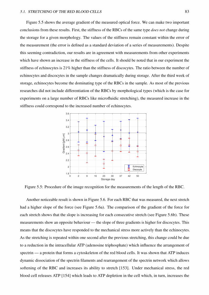
5.1. STRETCHING OF THE RED BLOOD CELLS 83
Figure 5.5 shows the average gradient of the measured optical force. We can make two important
conclusions from these results. First, the stiffness of the RBCs of the same type does not change during
the storage for a given morphology. The values of the stiffness remain constant within the error of
the measurement (the error is defined as a standard deviation of a series of measurements). Despite
this seeming contradiction, our results are in agreement with measurements from other experiments
which have shown an increase in the stiffness of the cells. It should be noted that in our experiment the
stiffness of echinocytes is 21% higher than the stiffness of discocytes. The ratio between the number of
echinocytes and discocytes in the sample changes dramatically during storage. After the third week of
storage, echinocytes become the dominating type of the RBCs in the sample. As most of the previous
researches did not include differentiation of the RBCs by morphological types (which is the case for
experiments on a large number of RBCs like microfluidic stretching), the measured increase in the
stiffness could correspond to the increased number of echinocytes.
0 2 9 16 23 30 37 42 50
Storage day
1.8
2
2.2
2.4
2.6
2.8
3
3.2
3.4
3.6
Gra
die
nt
[pN
/m
]
Echinocyte
Discocyte
Figure 5.5: Procedure of the image recognition for the measurements of the length of the RBC.
Another noticeable result is shown in Figure 5.6. For each RBC that was measured, the next stretch
had a higher slope of the force (see Figure 5.6a). The comparison of the gradient of the force for
each stretch shows that the slope is increasing for each consecutive stretch (see Figure 5.6b). These
measurements show an opposite behaviour — the slope of three gradients is higher for discocytes. This
means that the discocytes have responded to the mechanical stress more actively than the echinocytes.
As the stretching is repeated within one second after the previous stretching, this change could be due
to a reduction in the intracellular ATP (adenosine triphosphate) which influence the arrangement of
spectrin — a protein that forms a cytoskeleton of the red blood cells. It was shown that ATP induces
dynamic dissociation of the spectrin filaments and rearrangement of the spectrin network which allows
softening of the RBC and increases its ability to stretch [153]. Under mechanical stress, the red
blood cell releases ATP [154] which leads to ATP depletion in the cell which, in turn, increases the
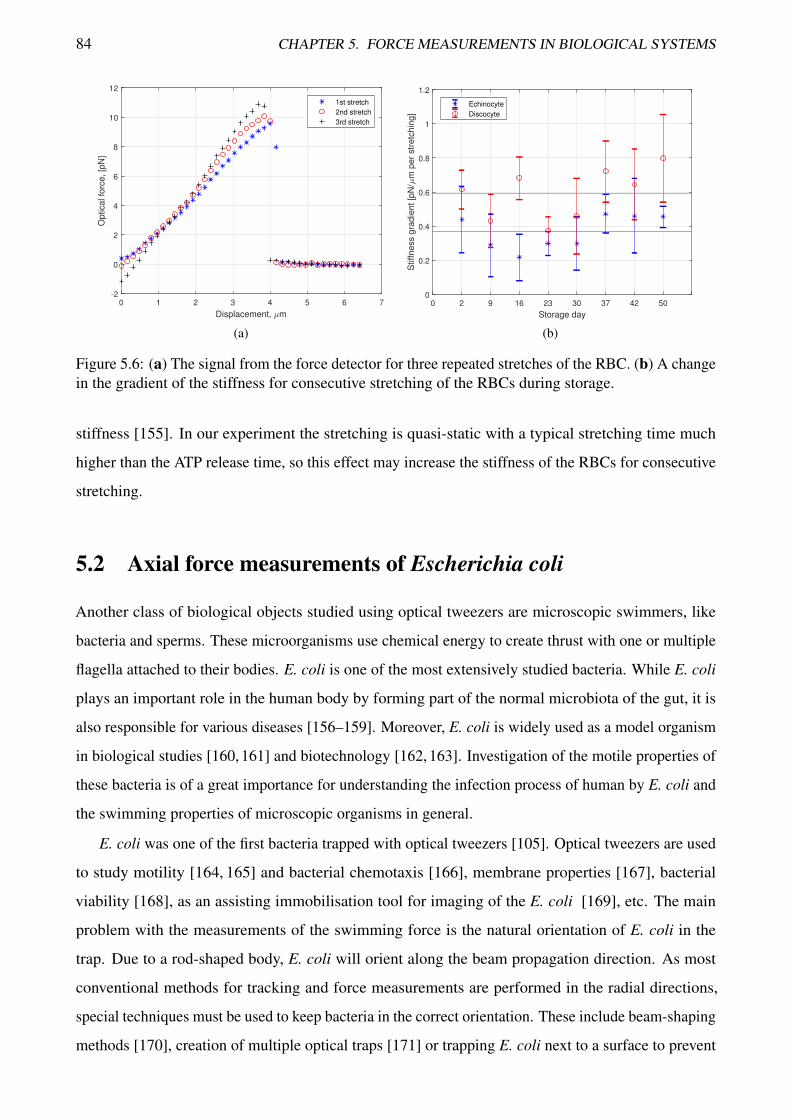
84 CHAPTER 5. FORCE MEASUREMENTS IN BIOLOGICAL SYSTEMS
0 1 2 3 4 5 6 7
Displacement, m
-2
0
2
4
6
8
10
12
Optical fo
rce, [p
N]
1st stretch
2nd stretch
3rd stretch
(a)
0 2 9 16 23 30 37 42 50
Storage day
0
0.2
0.4
0.6
0.8
1
1.2
Stiffness g
radie
nt [p
N/
m p
er
str
etc
hin
g]
Echinocyte
Discocyte
(b)
Figure 5.6: (a) The signal from the force detector for three repeated stretches of the RBC. (b) A changein the gradient of the stiffness for consecutive stretching of the RBCs during storage.
stiffness [155]. In our experiment the stretching is quasi-static with a typical stretching time much
higher than the ATP release time, so this effect may increase the stiffness of the RBCs for consecutive
stretching.
5.2 Axial force measurements of Escherichia coli
Another class of biological objects studied using optical tweezers are microscopic swimmers, like
bacteria and sperms. These microorganisms use chemical energy to create thrust with one or multiple
flagella attached to their bodies. E. coli is one of the most extensively studied bacteria. While E. coli
plays an important role in the human body by forming part of the normal microbiota of the gut, it is
also responsible for various diseases [156–159]. Moreover, E. coli is widely used as a model organism
in biological studies [160, 161] and biotechnology [162, 163]. Investigation of the motile properties of
these bacteria is of a great importance for understanding the infection process of human by E. coli and
the swimming properties of microscopic organisms in general.
E. coli was one of the first bacteria trapped with optical tweezers [105]. Optical tweezers are used
to study motility [164, 165] and bacterial chemotaxis [166], membrane properties [167], bacterial
viability [168], as an assisting immobilisation tool for imaging of the E. coli [169], etc. The main
problem with the measurements of the swimming force is the natural orientation of E. coli in the
trap. Due to a rod-shaped body, E. coli will orient along the beam propagation direction. As most
conventional methods for tracking and force measurements are performed in the radial directions,
special techniques must be used to keep bacteria in the correct orientation. These include beam-shaping
methods [170], creation of multiple optical traps [171] or trapping E. coli next to a surface to prevent
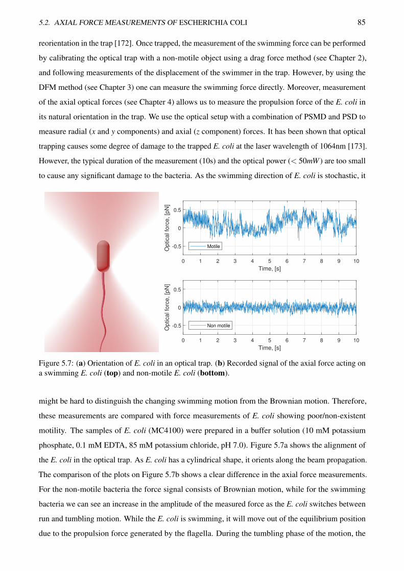
5.2. AXIAL FORCE MEASUREMENTS OF ESCHERICHIA COLI 85
reorientation in the trap [172]. Once trapped, the measurement of the swimming force can be performed
by calibrating the optical trap with a non-motile object using a drag force method (see Chapter 2),
and following measurements of the displacement of the swimmer in the trap. However, by using the
DFM method (see Chapter 3) one can measure the swimming force directly. Moreover, measurement
of the axial optical forces (see Chapter 4) allows us to measure the propulsion force of the E. coli in
its natural orientation in the trap. We use the optical setup with a combination of PSMD and PSD to
measure radial (x and y components) and axial (z component) forces. It has been shown that optical
trapping causes some degree of damage to the trapped E. coli at the laser wavelength of 1064nm [173].
However, the typical duration of the measurement (10s) and the optical power (< 50mW ) are too small
to cause any significant damage to the bacteria. As the swimming direction of E. coli is stochastic, it
0 1 2 3 4 5 6 7 8 9 10
Time, [s]
-0.5
0
0.5
Optical fo
rce, [p
N]
Motile
0 1 2 3 4 5 6 7 8 9 10
Time, [s]
-0.5
0
0.5
Optical fo
rce, [p
N]
Non motile
Figure 5.7: (a) Orientation of E. coli in an optical trap. (b) Recorded signal of the axial force acting ona swimming E. coli (top) and non-motile E. coli (bottom).
might be hard to distinguish the changing swimming motion from the Brownian motion. Therefore,
these measurements are compared with force measurements of E. coli showing poor/non-existent
motility. The samples of E. coli (MC4100) were prepared in a buffer solution (10 mM potassium
phosphate, 0.1 mM EDTA, 85 mM potassium chloride, pH 7.0). Figure 5.7a shows the alignment of
the E. coli in the optical trap. As E. coli has a cylindrical shape, it orients along the beam propagation.
The comparison of the plots on Figure 5.7b shows a clear difference in the axial force measurements.
For the non-motile bacteria the force signal consists of Brownian motion, while for the swimming
bacteria we can see an increase in the amplitude of the measured force as the E. coli switches between
run and tumbling motion. While the E. coli is swimming, it will move out of the equilibrium position
due to the propulsion force generated by the flagella. During the tumbling phase of the motion, the
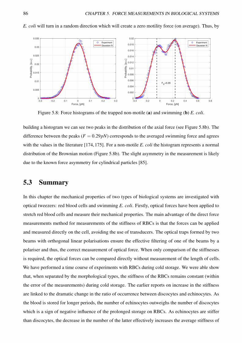
86 CHAPTER 5. FORCE MEASUREMENTS IN BIOLOGICAL SYSTEMS
E. coli will turn in a random direction which will create a zero motility force (on average). Thus, by
-0.3 -0.2 -0.1 0 0.1 0.2 0.3
Force, [pN]
0
0.005
0.01
0.015
0.02
0.025
0.03
0.035
Pro
ba
bili
ty,
[a.u
.]
Experiment
Gaussian fit
-0.4 -0.2 0 0.2 0.4 0.6 0.8
Force, [pN]
0
0.002
0.004
0.006
0.008
0.01
0.012
0.014
0.016
0.018
0.02
Pro
ba
bili
ty,
[a.u
.]
FS
=0.29
Experiment
Gaussian fit
Figure 5.8: Force histograms of the trapped non-motile (a) and swimming (b) E. coli.
building a histogram we can see two peaks in the distribution of the axial force (see Figure 5.8b). The
difference between the peaks (F = 0.29pN) corresponds to the averaged swimming force and agrees
with the values in the literature [174, 175]. For a non-motile E. coli the histogram represents a normal
distribution of the Brownian motion (Figure 5.8b). The slight asymmetry in the measurement is likely
due to the known force asymmetry for cylindrical particles [85].
5.3 Summary
In this chapter the mechanical properties of two types of biological systems are investigated with
optical tweezers: red blood cells and swimming E. coli. Firstly, optical forces have been applied to
stretch red blood cells and measure their mechanical properties. The main advantage of the direct force
measurements method for measurements of the stiffness of RBCs is that the forces can be applied
and measured directly on the cell, avoiding the use of transducers. The optical traps formed by two
beams with orthogonal linear polarisations ensure the effective filtering of one of the beams by a
polariser and thus, the correct measurement of optical force. When only comparison of the stiffnesses
is required, the optical forces can be compared directly without measurement of the length of cells.
We have performed a time course of experiments with RBCs during cold storage. We were able show
that, when separated by the morphological types, the stiffness of the RBCs remains constant (within
the error of the measurements) during cold storage. The earlier reports on increase in the stiffness
are linked to the dramatic change in the ratio of occurrence between discocytes and echinocytes. As
the blood is stored for longer periods, the number of echinocytes outweighs the number of discocytes
which is a sign of negative influence of the prolonged storage on RBCs. As echinocytes are stiffer
than discocytes, the decrease in the number of the latter effectively increases the average stiffness of
5.3. SUMMARY 87
the RBCs in the sample over time. Another sign of decreased functionality of the echinocytes is the
response to repeated mechanical stress. Based on previous works that have shown a link between the
concentration of the ATP in a cell and its stiffness, we can hypothesise that the depletion of the ATP is
responsible for the smaller increase in the stiffness of the RBCs for each subsequent stretch. However,
additional experiments are required to confirm this hypothesis.
Secondly, the propulsion force generated by E. coli is measured. The swimming forces of motile
bacteria, like E. coli , can be measured with an axial filter mask using position sensitive masked
detector. The proof-of-principle experiments show that one can measure the propulsion force of the
motile organisms using the direct force measurement method in combination with a position sensitive
masked detector. This force measurements can be performed in all three axes and thus, remove the
necessity of beam-shaping or other techniques being applied to align bacteria in the trap.

Chapter 6
Conclusions
Optical tweezers, as a versatile tool for applying and measuring forces, is widely used in different
micro- and nanosystems. The forces in optical tweezers are in the piconewton range which makes
them suitable for applications in various microscopic biological systems, such as cells and bacteria.
In this thesis force measurement techniques in optical tweezers and their applications in biological
systems are investigated.
Optical trapping is due to the optical gradient force. When an object is placed in the optical
gradient the restoring force appears as a result of a change of the momentum of the trapping light. This
restoring force pushes a trapped particle back to the equilibrium position and thus, creates an optical
trap. Optical forces can be calculated numerically using different methods and approximations which
are specific to experimental parameters of the system. Simulations of optical tweezers are important
for design of the trapping system and interpretation of experimental results. As this thesis considers
microscopic biological objects, a typical size of the trapped particles is within or greater than a trapping
wavelength. Therefore, in most situations a full-wave solution of Maxwell’s equations is required. In
the case of larger objects the geometrical optics approximation can be utilised. To perform simulations
of optical trapping freely available computational toolboxes can be used [22, 31]. However, as many
biological objects are flexible, an implementation of a toolbox for calculation of optical forces acting
on deformable particles will significantly improve our understanding of experimental outcome for
such objects.
Among the other trapping configurations, holographically controlled single- and multi-beam optical
tweezers are the best choice for microscopic biological entities, such as cells and living organisms.
Such optical systems give good dynamical control of the trap and allow application and measurement
of the forces inside biological objects.
If a trapped particle stays in a linear range of the force–position curve the measurement of the force89
90 CHAPTER 6. CONCLUSIONS
can be performed by tracking the position of the particle. However, with the position-based approaches
a calibration for each particle in the trap is required. If the trapping beam, or the trapped particle, has
been changed a recalibration is necessary.
An alternative way of measuring optical forces is the direct force measurement method which uses
the determination of the momentum change of the trapping beam. This method requires a high-NA
objective to collect most of the scattered light. In order to measure the optical force, a detector with
appropriate intensity transfer function should be placed in a back focal plane of the condenser. While
the direct force measurement method implies calibration-free measurements, the initial calibration
of the force detector is required. It can be performed with simultaneous measurements of the optical
force (with uncalibrated force detector) and position of the particle (with a position detector or camera).
Chapter 3 describes in detail a calibration procedure for radial forces using thermal motion of the
trapped particle. The experiments show that such calibration is robust across different particles,
trapping mediums, and trapping beams. The particle can be non-spherical, birefringent, or even change
shape or size over the course of the measurements. This is a great advantage for biological systems as
often they are non-spherical and flexible objects which makes conventional position-based methods of
force measurements unpractical to use.
In the direct force measurement method a duo-lateral position sensitive detector can be used to
measure radial components of the optical force but such a detector is unable to measure axial forces.
In Chapter 4 a position sensitive masked detector (PSMD) based on digital micromirror device has
been proposed. The PSMD allows high-bandwidth detection of both radial and axial components
of the optical force. As the digital micromirror device allows dynamical control of the pattern, the
simultaneous measurements of axial and radial forces with a single PSMD are possible using a time-
sharing approach. I have shown that a combination of duo-lateral position sensitive detector and PSMD
can be used to measure the three-dimensional distribution of the forces in an optical trap.
Calibration of the axial force detector (i.e. the PSMD with a mask for axial force measurements)
is more complicated as the position of the particle along the z-axis (orthogonal to the viewing plane)
is required. However, as the digital micromirror device allows replacement of the amplitude pattern
under the same conditions, the axial calibration constant can be determined using the mask for radial
force measurements. The performance of the proposed position sensitive masked detector for the axial
optical forces measurements was estimated using the Stokes drag force acting on a trapped particle
in a fluid flow. The results show excellent linearity for the different velocities and little spread in the
measurements.
Finally, all the developments in design of the trapping system, calibration of the trap, and force
detection were applied to biological systems. The two sets of experiments include measurement of the
91
mechanical properties of the human red blood cells during cold storage and measurement of the thrust
generated by a swimming E. coli bacterium.
The first set of experiments was performed on red blood cells. A dual-beam optical tweezers with
spatial light modulator for holographic control of the trap has been used to investigate the mechanical
properties of red blood cells during cold storage. The advantage of the direct force measurement
method in such systems is that the forces can be applied and measured without any force transducers
directly on the cell. The results of the time-course of experiments have shown that, when separated
by the morphological types (discocytes and echinocytes), the stiffness of the cells remains constant
during storage. The commonly observed increase in the stiffness is likely due to the change in the
ratio of occurrence between discocytes (normal cells) and echinocytes (damaged cells). For longer
storage periods the number of echinocytes greatly outweighs the number of discocytes. Moreover, the
response of the cells to a repeated mechanical stress is much lower in echinocytes which is also a sign
of degradation in functionality. This implies that changes in the stiffness and ability of the cells to
respond to the stress are directly reflected in morphological changes of the cells.
These experiments give a better understanding of the behaviour of red blood cells during their
life-cycle and storage. However, many questions about the processes in red blood cells require
additional experiments. For example, it was shown that the mechanical stiffness of the cell depends
on concentration of ATP in the cell. The measurements of the cell’s response to a stress of different
frequencies will reveal dynamical characteristics of the membrane and its link to the change in ATP
consumption rates. Moreover, the methods used for measuring stiffness in red blood cells can be
extended to other cells and tissues assuming that the optical forces are strong enough to stretch the cell
or to move a cell-cell junction.
Although the optical trapping setup satisfies all the requirements for the trapping of biological
entities, the experiments with red blood cells are very time-consuming which significantly reduces the
possible number of measurements. The implementation of a microfluidic flow chamber and automation
of a cell selection and trapping process is a possible solution.
The second set of experiments was devoted to the measurement of the thrust generated by a
swimming E. coli. A common complication with the measurements of the E. coli propulsion force is
the orientation of the bacterium in the trap. As E. coli is a cylindrically shaped bacterium, it orients
along the beam propagation axis and often either a beam shaping technique or trapping next to a
surface is required to perform measurements. However, the propulsion force can be measured directly
in the natural orientation of E. coli in the trap using the position sensitive masked detector. While this
proof-of-principle experiment shows the ability of the PSMD to provide axial force measurements,
it is not limited to E. coli and can be performed on other swimmers, e.g., sperms. Of course, further

92 CHAPTER 6. CONCLUSIONS
experiments with biological swimmers are required and will help to answer many important questions
on the hydrodynamics of flagellar motion and the operating principles of the molecular motors which
move life.
Bibliography
[1] A. Ashkin. Acceleration and Trapping of Particles by Radiation Pressure. Physical Review
Letters, 24(4):156–159, Jan 1970.
[2] A. Ashkin, J. M. Dziedzic, J. E. Bjorkholm, and S. Chu. Observation of a single-beam gradient
force optical trap for dielectric particles. Optics Letters, 11(5):288–290, May 1986.
[3] W. D. Phillips. Nobel Lecture: Laser cooling and trapping of neutral atoms. Reviews of Modern
Physics, 70(3):721–741, Jul 1998.
[4] A. Hochstetter and T. Pfohl. Motility, Force Generation, and Energy Consumption of Unicellular
Parasites. Trends in Parasitology, 32(7):531–541, Jul 2016.
[5] K. P. Sigdel, A. E. Pittman, T. R. Matin, and G. M. King. High-resolution afm-based force
spectroscopy. In Y. L. Lyubchenko, editor, Nanoscale Imaging: Methods and Protocols, pages
49–62. Springer New York, New York, NY, 2018.
[6] A. B. Churnside, R. M. A. Sullan, D. M. Nguyen, S. O. Case, M. S. Bull, G. M. King, and
T. T. Perkins. Routine and Timely Sub-picoNewton Force Stability and Precision for Biological
Applications of Atomic Force Microscopy. Nano Letters, 12(7):3557–3561, Jul 2012.
[7] J. K. Faulk, D. T. Edwards, M. S. Bull, and T. T. Perkins. Chapter Thirteen - Improved
Force Spectroscopy Using Focused-Ion-Beam-Modified Cantilevers. Methods in Enzymology,
582:321–351, Jan 2017.
[8] D. T. Edwards and T. T. Perkins. Optimizing force spectroscopy by modifying commercial
cantilevers: Improved stability, precision, and temporal resolution. Journal of Structural Biology,
197(1):13–25, Jan 2017.
[9] U. Lucia. Bioengineering thermodynamics of biological cells. Theoretical Biology & Medical
Modelling, 12, 2015.93
94 BIBLIOGRAPHY
[10] A. E. Smith, L. Z. Zhou, A. H. Gorensek, M. Senske, and G. J. Pielak. In-cell thermodynam-
ics and a new role for protein surfaces. Proceedings of the National Academy of Sciences,
113(7):1725–1730, Feb 2016.
[11] D. Huber, A. Oskooei, X. Casadevall i. Solvas, A. DeMello, and G. V. Kaigala. Hydrodynamics
in Cell Studies. Chemical Reviews, 118(4):2042–2079, Feb 2018.
[12] E. Lauga. Bacterial Hydrodynamics. Annual Review of Fluid Mechanics, 48(1):105–130, Jan
2016.
[13] W. C. K. Poon and D. Andelman. Soft Condensed Matter Physics in Molecular and Cell Biology
(Scottish Graduate Series). CRC Press, Jan 2006.
[14] U. Schwarz. Soft matters in cell adhesion: rigidity sensing on soft elastic substrates. Soft Matter,
3(3):263–266, Feb 2007.
[15] J. R. Moffitt, Y. R. Chemla, S. B. Smith, and C. Bustamante. Recent advances in optical
tweezers. Annual Review of Biochemistry, 77:205–28, 2008.
[16] T. L. Min, P. J. Mears, L. M. Chubiz, C. V. Rao, I. Golding, and Y. R. Chemla. High-
resolution, long-term characterization of bacterial motility using optical tweezers. Nature
Methods, 6(11):831, Oct 2009.
[17] A. A. Bui, A. B. Stilgoe, I. C. Lenton, L. J. Gibson, A. V. Kashchuk, S. Zhang, H. Rubinsztein-
Dunlop, and T. A. Nieminen. Theory and practice of simulation of optical tweezers. Journal of
Quantitative Spectroscopy and Radiative Transfer, 195:66–75, 2017. Laser-light and Interactions
with Particles 2016.
[18] R. C. Gauthier. Computation of the optical trapping force using an FDTD based technique.
Optics Express, 13(10):3707–3718, May 2005.
[19] I. C. D. Lenton, A. B. Stilgoe, H. Rubinsztein-Dunlop, and T. A. Nieminen. Visual guide to
optical tweezers. European Journal of Physics, 38(3):034009, Mar 2017.
[20] V. L. Y. Loke, T. A. Nieminen, S. J. Parkin, N. R. Heckenberg, and H. Rubinsztein-Dunlop.
FDFD/T-matrix hybrid method. Journal of Quantitative Spectroscopy and Radiative Transfer,
106(1):274–284, Jul 2007.
[21] Y. Harada and T. Asakura. Radiation forces on a dielectric sphere in the Rayleigh scattering
regime. Optics Communications, 124(5):529–541, Mar 1996.

BIBLIOGRAPHY 95
[22] A. Callegari, M. Mijalkov, A. B. Gokoz, and G. Volpe. Computational toolbox for optical
tweezers in geometrical optics. JOSA B, 32(5):B11–B19, May 2015.
[23] G. Gouesbet and G. Grehan. Generalized Lorenz-Mie Theories. Springer, Cham, 2017.
[24] J. A. Lock and G. Gouesbet. Generalized Lorenz–Mie theory and applications. Journal of
Quantitative Spectroscopy and Radiative Transfer, 110(11):800–807, Jul 2009.
[25] T. A. Nieminen, H. Rubinsztein-Dunlop, and N. R. Heckenberg. Calculation of the T-matrix:
general considerations and application of the point-matching method. Journal of Quantitative
Spectroscopy and Radiative Transfer, 79–80:1019–1029, Jun 2003.
[26] T. A. Nieminen, V. L. Loke, A. B. Stilgoe, N. R. Heckenberg, and H. Rubinsztein-Dunlop.
T-matrix method for modelling optical tweezers. Journal of Modern Optics, 58(5-6):528–544,
2011.
[27] D. W. Mackowski and M. I. Mishchenko. Calculation of the T matrix and the scattering matrix
for ensembles of spheres. JOSA A, 13(11):2266–2278, Nov 1996.
[28] A. Doicu and T. Wriedt. Computation of the beam-shape coefficients in the generalized
Lorenz–Mie theory by using the translational addition theorem for spherical vector wave
functions. Applied Optics, 36(13):2971–2978, May 1997.
[29] T. A. Nieminen, H. Rubinsztein-Dunlop, and N. R. Heckenberg. Multipole expansion of
strongly focussed laser beams. Journal of Quantitative Spectroscopy and Radiative Transfer,
79–80:1005–1017, Jun 2003.
[30] P. C. Waterman. Matrix formulation of electromagnetic scattering. Proceedings of the IEEE,
53(8):805–812, Aug 1965.
[31] T. A. Nieminen, V. L. Y. Loke, A. B. Stilgoe, G. Knoner, A. M. Branczyk, N. R. Heckenberg,
and H. Rubinsztein-Dunlop. Optical tweezers computational toolbox. Journal of Optics A: Pure
and Applied Optics, 9(8):S196, 2007.
[32] A. B. Stilgoe, A. V. Kashchuk, D. Preece, and H. Rubinsztein-Dunlop. An interpretation
and guide to single-pass beam shaping methods using SLMs and DMDs. Journal of Optics,
18(6):065609, 2016.
[33] M. A. Taylor, M. Waleed, A. B. Stilgoe, H. Rubinsztein-Dunlop, and W. P. Bowen. Enhanced
optical trapping via structured scattering. Nature Photonics, 9(10):669, Aug 2015.
96 BIBLIOGRAPHY
[34] S. B. Smith, Y. Cui, and C. Bustamante. Optical-trap force transducer that operates by direct
measurement of light momentum. Methods Enzymology, 361:134–162, Jan 2003.
[35] M. Ribezzi-Crivellari, J. M. Huguet, and F. Ritort. Counter-propagating dual-trap optical tweez-
ers based on linear momentum conservation. Review of Scientific Instruments, 84(4):043104–10,
Apr 2013.
[36] T. Cizmar, V. Garces-Chavez, K. Dholakia, and P. Zemanek. Optical trapping in counter-
propagating Bessel beams. Optical Trapping and Optical Micromanipulation, 5514:643–652,
Oct 2004.
[37] D. Grass, J. Fesel, S. G. Hofer, N. Kiesel, and M. Aspelmeyer. Optical trapping and control
of nanoparticles inside evacuated hollow core photonic crystal fibers. Applied Physics Letters,
108(22):221103, May 2016.
[38] P. Domachuk, N. Wolchover, M. Cronin-Golomb, and F. G. Omenetto. Effect of hollow-core
photonic crystal fiber microstructure on transverse optical trapping. Applied Physics Letters,
94(14):141101–3, Apr 2009.
[39] D. S. Bykov, S. Xie, R. Zeltner, A. Machnev, G. K. L. Wong, T. G. Euser, and P. St. J. Russell.
Long-range optical trapping and binding of microparticles in hollow-core photonic crystal fibre.
Light: Science & Applications, 7(1):22, Jun 2018.
[40] M. Pitzek, R. Steiger, G. Thalhammer, S. Bernet, and M. Ritsch-Marte. Optical mirror trap with
a large field of view. Optics Express, 17(22):19414–19423, Oct 2009.
[41] M. C. Gower. Phase Conjugate Mirrors. Physics Bulletin, 38(6):220, Jun 1987.
[42] M. Woerdemann, K. Berghoff, and C. Denz. Dynamic multiple-beam counter-propagating
optical traps using optical phase-conjugation. Optics Express, 18(21):22348–22357, Oct 2010.
[43] W. Wang, A. E. Chiou, G. J. Sonek, and M. W. Berns. Self-aligned dual-beam optical laser trap
using photorefractive phase conjugation. JOSA B, 14(4):697–704, Apr 1997.
[44] N. P. Mauranyapin, L. S. Madsen, M. A. Taylor, M. Waleed, and W. P. Bowen. Evanescent
single-molecule biosensing with quantum-limited precision. Nature Photonics, 11(8):477, Jun
2017.
[45] M. L. Juan, M. Righini, and R. Quidant. Plasmon nano-optical tweezers. Nature Photonics,
5(6):349, Jun 2011.
BIBLIOGRAPHY 97
[46] A. Zehtabi-Oskuie, H. Jiang, B. R. Cyr, D. W. Rennehan, A. A. Al-Balushi, and R. Gordon.
Double nanohole optical trapping: dynamics and protein-antibody co-trapping. Lab on a Chip,
13(13):2563–2568, Jun 2013.
[47] A. A. Al Balushi, A. Kotnala, S. Wheaton, R. M. Gelfand, Y. Rajashekara, and R. Gordon.
Label-free free-solution nanoaperture optical tweezers for single molecule protein studies.
Analyst, 140(14):4760–4778, 2015.
[48] T. Yoshikawa, M. Tamura, S. Tokonami, and T. Iida. Optical Trap-Mediated High-Sensitivity
Nanohole Array Biosensors with Random Nanospikes. Journal of Physical Chemistry Letters,
8(2):370–374, Jan 2017.
[49] S. N. S. Reihani, S. A. Mir, A. C. Richardson, and L. B. Oddershede. Significant improvement of
optical traps by tuning standard water immersion objectives. Journal of Optics, 13(10):105301,
Sep 2011.
[50] R. Parthasarathy. Rapid, accurate particle tracking by calculation of radial symmetry centers.
Nature Methods, 9:724, 2012.
[51] E.-L. Florin, A. Pralle, E. Stelzer, and J. Horber. Photonic force microscope calibration by
thermal noise analysis. Applied Physics A, 66(1):S75–S78, 1998.
[52] K. Berg-Sørensen and H. Flyvbjerg. Power spectrum analysis for optical tweezers. Review of
Scientific Instruments, 75(3):594–612, 2004.
[53] S. F. Tolic-Nørrelykke, E. Schaffer, J. Howard, F. S. Pavone, F. Julicher, and H. Flyvbjerg.
Calibration of optical tweezers with positional detection in the back focal plane. Review of
Scientific Instruments, 77(10):103101, 2006.
[54] W. H. Wright, G. J. Sonek, and M. W. Berns. Parametric study of the forces on microspheres
held by optical tweezers. Applied Optics, 33(9):1735–1748, 1994.
[55] H. Felgner, O. Muller, and M. Schliwa. Calibration of light forces in optical tweezers. Applied
Optics, 34(6):977–982, 1995.
[56] J. J. Waterston and J. W. Strutt. I. On the physics of media that are composed of free and
perfectly elastic molecules in a state of motion. Philosophical Transactions of the Royal Society,
183:1–79, Jan 1892.
[57] Lord Rayleigh. VI. The law of partition of kinetic energy. London, Edinburgh, and Dublin
Philosophical Magazine and Journal of Science, 49(296):98–118, Jan 1900.
98 BIBLIOGRAPHY
[58] L. D. Landau, E. M. Lifshitz, L. P. Pitaevskii, J. B. Sykes, and M. J. Kearsley. Statistical Physics.
Elsevier Science & Technology, Oxford, United Kingdom, 2013.
[59] M. Sarshar, W. Wong, and B. Anvari. Comparative study of methods to calibrate the stiffness of
a single-beam gradient-force optical tweezers over various laser trapping powers. Journal of
Biomedical Optics, 19(11):115001, Nov 2014.
[60] M. Andersson, F. Czerwinski, and L. B. Oddershede. Optimizing active and passive calibration
of optical tweezers. Journal of Optics, 13(4):044020, Mar 2011.
[61] K. Berg-Sørensen, E. J. G. Peterman, T. Weber, C. F. Schmidt, and H. Flyvbjerg. Power
spectrum analysis for optical tweezers. II: Laser wavelength dependence of parasitic filtering,
and how to achieve high bandwidth. Review of Scientific Instruments, 77(6):063106, 2006.
[62] Y. Deng, J. Bechhoefer, and N. R. Forde. Brownian motion in a modulated optical trap. Journal
of Optics A: Pure and Applied Optics, 9(8):S256, Jul 2007.
[63] M. Fischer and K. Berg-Sørensen. Calibration of trapping force and response function of optical
tweezers in viscoelastic media. Journal of Optics A: Pure and Applied Optics, 9(8):S239, Jul
2007.
[64] G. Volpe and G. Volpe. Simulation of a Brownian particle in an optical trap. American Journal
of Physics, 81(3):224, Feb 2013.
[65] A. van der Horst and N. R. Forde. Power spectral analysis for optical trap stiffness calibration
from high-speed camera position detection with limited bandwidth. Optics Express, 18(8):7670–
7677, Apr 2010.
[66] P. M. Hansen, I. M. Tolic-Nørrelykke, H. Flyvbjerg, and K. Berg-Sørensen. tweezercalib 2.0:
Faster version of MatLab package for precise calibration of optical tweezers. Computer Physics
Communications, 174(6):518–520, Mar 2006.
[67] E.-L. Florin, A. Pralle, E. H. K. Stelzer, and J. K. H. Horber. Photonic force microscope
calibration by thermal noise analysis. Applied Physics A, 66(1):S75–S78, 2018.
[68] A. A. M. Bui, A. V. Kashchuk, M. A. Balanant, T. A. Nieminen, H. Rubinsztein-Dunlop, and
A. B. Stilgoe. Calibration of force detection for arbitrarily shaped particles in optical tweezers.
Scientific Reports, 8(1):10798, Jul 2018.
BIBLIOGRAPHY 99
[69] C. O. Mejean, A. W. Schaefer, E. A. Millman, P. Forscher, and E. R. Dufresne. Multiplexed force
measurements on live cells with holographic optical tweezers. Optics Express, 17(8):6209–6217,
Apr 2009.
[70] H. Zhang and K.-K. Liu. Optical tweezers for single cells. Journal of the Royal Society Interface,
5(24):671–690, Jul 2008.
[71] A. Farre, F. Marsa, and M. Montes-Usategui. Optimized back-focal-plane interferometry
directly measures forces of optically trapped particles. Optics Express, 20(11):12270–12291,
May 2012.
[72] A. Farre and M. Montes-Usategui. A force detection technique for single-beam optical traps
based on direct measurement of light momentum changes. Optics Express, 18(11):11955–11968,
May 2010.
[73] G. Thalhammer, L. Obmascher, and M. Ritsch-Marte. Direct measurement of axial optical
forces. Optics Express, 23(5):6112–29, 2015.
[74] E. Abbe. VII. On the estimation of aperture in the microscope. Journal of the Royal Microscop-
ical Society, 1(3):388–423, Jun 1881.
[75] D. Chen, B. Lin, and Y. Chen. Fabrication and characterization of two-dimensional pin-cushion
position sensitive detectors. Chinese Optics Letters, 2(7):426–427, Jul 2004.
[76] P. S. Bui and N. D. Taneja. Tetra-lateral position sensing detector. United States Patents,
US8399909B2, May 2010.
[77] D. J. W. Noorlag, S. Middelhoek, D. J. W. Noorlag, and S. Middelhoek. Two-dimensional
position-sensitive photodetector with high linearity made with standard i.c.-technology. IEEE
Journal on Solid-State and Electron Devices, 3(3):75–82, May 1979.
[78] S. Cui and Y. C. Soh. The effect of spot size on linearity improvement of tetra-lateral position
sensitive detector. Optical and Quantum Electronics, 42(11-13):721, 2011.
[79] W. Wang, I. J. Busch-Vishniac, W. Wang, and I. J. Busch-Vishniac. The linearity and sensitivity
of lateral effect position sensitive devices-an improved geometry. IEEE Transactions on Electron
Devices, 36(11):2475–2480, Nov 1989.
[80] R. Huang, I. Chavez, K. M. Taute, B. Lukic, S. Jeney, M. G. Raizen, and E.-L. Florin. Direct
observation of the full transition from ballistic to diffusive Brownian motion in a liquid. Nature
Physics, 7:576, 2011.
100 BIBLIOGRAPHY
[81] G. M. Gibson, J. Leach, S. Keen, A. J. Wright, and M. J. Padgett. Measuring the accuracy
of particle position and force in optical tweezers using high-speed video microscopy. Optics
Express, 16(19):14561–14570, Sep 2008.
[82] P. Barak, A. Rai, P. Rai, and R. Mallik. Quantitative optical trapping on single organelles in cell
extract. Nature Methods, 10:68, 2012.
[83] S. B. Smith, Y. Cui, and C. Bustamante. Overstretching B-DNA: the elastic response of
individual double-stranded and single-stranded DNA molecules. Science, 271(5250):795–9,
1996.
[84] R. S. Dutra, N. B. Viana, P. A. Maia Neto, and H. M. Nussenzveig. Absolute calibration of
forces in optical tweezers. Physical Review A, 90(1):013825, 2014.
[85] A. A. M. Bui, A. B. Stilgoe, T. A. Nieminen, and H. Rubinsztein-Dunlop. Calibration of
nonspherical particles in optical tweezers using only position measurement. Optics Letters,
38(8):1244–1246, 2013.
[86] S. Kuo and M. Sheetz. Force of single kinesin molecules measured with optical tweezers.
Science, 260(5105):232–234, 1993.
[87] A. A. Bui, A. B. Stilgoe, N. Khatibzadeh, T. A. Nieminen, M. W. Berns, and H. Rubinsztein-
Dunlop. Escape forces and trajectories in optical tweezers and their effect on calibration. Optics
Express, 23(19):24317–30, 2015.
[88] M. Josep, C. R. Andrew, S. N. S. Reihani, B. O. Lene, and B.-S. Kirstine. Quantitative
determination of optical trapping strength and viscoelastic moduli inside living cells. Physical
Biology, 10(4):046006, 2013.
[89] N. Khatibzadeh, A. B. Stilgoe, A. A. Bui, Y. Rocha, G. M. Cruz, V. Loke, L. Z. Shi, T. A.
Nieminen, H. Rubinsztein-Dunlop, and M. W. Berns. Determination of motility forces on
isolated chromosomes with laser tweezers. Scientific Reports, 4:6866, 2014.
[90] A. J. Weinheimer. Application of the Stokes drag on spheroids to the drag on disks and cylinders.
Journal of the Atmospheric Sciences, 44(18):2674–2676, 1987.
[91] D. Maugeri, P. Panebianco, V. Cilmi, A. Bruno, G. Receputo, A. Salerno, M. Motta, M. G.
Napolitano, and M. S. Russo. Alterations of blood and plasma viscosity and erythrocyte filtration
in senile osteoporosis. Archives of Gerontology and Geriatrics, 19(1):75–82, 1994.
BIBLIOGRAPHY 101
[92] S. J. Parkin, R. Vogel, M. Persson, M. Funk, V. L. Y. Loke, T. A. Nieminen, N. R. Heckenberg,
and H. Rubinsztein-Dunlop. Highly birefringent vaterite microspheres: production, characteri-
zation and applications for optical micromanipulation. Optics Express, 17(24):21944–21955,
2009.
[93] A. I. Bishop, T. A. Nieminen, N. R. Heckenberg, and H. Rubinsztein-Dunlop. Optical mi-
crorheology using rotating laser-trapped particles. Physical Review Letters, 92(19):198104,
2004.
[94] L. Friedrich and A. Rohrbach. Surface imaging beyond the diffraction limit with optically
trapped spheres. Nature Nanotechnology, 10:1064, 2015.
[95] S. S. B. Bustamante, Carlos J. Light-force sensor and method for measuring axial optical-trap
forces from changes in light momentum along an optic axis. United States Patents, 7133132,
2006.
[96] A. Farre, F. Marsa, and M. Montes-Usategui. Beyond the hookean spring model: Direct
measurement of optical forces through light momentum changes. In Optical Tweezers: Methods
and Protocols, pages 41–76. Humana Press, New York, NY, 2017.
[97] I. Chavez, R. Huang, K. Henderson, E.-L. Florin, and M. G. Raizen. Development of a fast
position-sensitive laser beam detector. Review of Scientific Instruments, 79(10):105104–3, Oct
2008.
[98] J. S. Dana Dudley, Walter M. Duncan. Emerging digital micromirror device (DMD) applications.
In MOEMS Display and Imaging Systems, volume 4985, pages 14–25, 2003.
[99] G. Gauthier, I. Lenton, N. M. Parry, M. Baker, M. J. Davis, H. Rubinsztein-Dunlop, and T. W.
Neely. Direct imaging of a digital-micromirror device for configurable microscopic optical
potentials. Optica, 3(10):1136–1143, Oct 2016.
[100] L. Schuchman. Dither signals and their effect on quantization noise. IEEE Transactions on
Communication Technology, 12(4):162–165, December 1964.
[101] K. Norregaard, R. Metzler, C. M. Ritter, K. Berg-Sørensen, and L. B. Oddershede. Manipulation
and Motion of Organelles and Single Molecules in Living Cells. Chemical Reviews, 117(5):4342–
4375, Mar 2017.
102 BIBLIOGRAPHY
[102] C. Hawes, A. Osterrieder, I. A. Sparkes, and T. Ketelaar. Optical tweezers for the micromanipu-
lation of plant cytoplasm and organelles. Current Opinion in Plant Biology, 13(6):731–735,
Dec 2010.
[103] U. Bockelmann, Ph. Thomen, B. Essevaz-Roulet, V. Viasnoff, and F. Heslot. Unzipping
DNA with optical tweezers: high sequence sensitivity and force flips. Biophysical Journal,
82(3):1537–1553, Mar 2002.
[104] U. F. Keyser, J. van der Does, C. Dekker, and N. H. Dekker. Optical tweezers for force
measurements on DNA in nanopores. Review of Scientific Instruments, 77(10):105105–9, Oct
2006.
[105] A. Ashkin, J. M. Dziedzic, and T. Yamane. Optical trapping and manipulation of single cells
using infrared laser beams. Nature, 330(6150):769, Dec 1987.
[106] M.-C. Zhong, X.-B. Wei, J.-H. Zhou, Z.-Q. Wang, and Y.-M. Li. Trapping red blood cells in
living animals using optical tweezers. Nature Communications, 4:1768, Apr 2013.
[107] H. M. Nussenzveig. Cell membrane biophysics with optical tweezers. European Biophysics
Journal, 47(5):499–514, Jul 2018.
[108] H. Guo, Q. Cao, D. Ren, G. Liu, J. Duan, Z. Li, D. Zhang, and X. Han. Measurements
of leucocyte membrane elasticity based on the optical tweezers. Chinese Science Bulletin,
48(5):503–508, Mar 2003.
[109] F. Qian, S. Ermilov, D. Murdock, W. E. Brownell, and B. Anvari. Combining optical tweezers
and patch clamp for studies of cell membrane electromechanics. Review of Scientific Instruments,
75(9):2937–2942, Sep 2004.
[110] D. Mizuno, C. Tardin, C. F. Schmidt, and F. C. MacKintosh. Nonequilibrium Mechanics of
Active Cytoskeletal Networks. Science, 315(5810):370–373, Jan 2007.
[111] K. Svoboda, C. F. Schmidt, B. J. Schnapp, and S. M. Block. Direct observation of kinesin
stepping by optical trapping interferometry. Nature, 365(6448):721, Oct 1993.
[112] C. Veigel and C. F. Schmidt. Moving into the cell: single-molecule studies of molecular motors
in complex environments. Nature Reviews Molecular Cell Biology, 12(3):163, Feb 2011.
[113] L. B. Oddershede. Force probing of individual molecules inside the living cell is now a reality.
Nature Chemical Biology, 8(11):879, Oct 2012.
BIBLIOGRAPHY 103
[114] S. Peter Klinken. Red blood cells. International Journal of Biochemistry & Cell Biology,
34(12):1513–1518, Dec 2002.
[115] L. Pan, R. Yan, W. Li, and K. Xu. Super-resolution microscopy reveals the native ultrastructure
of the erythrocyte cytoskeleton. Cell Reports, 22(5):1151–1158, Jan 2018.
[116] V. Bennett. The spectrin-actin junction of erythrocyte membrane skeletons. Biochimica et
Biophysica Acta (BBA) - Reviews on Biomembranes, 988(1):107–121, Jan 1989.
[117] S. V. Rudenko. Erythrocyte morphological states, phases, transitions and trajectories. Biochimica
et Biophysica Acta (BBA) - Biomembranes, 1798(9):1767–1778, Sep 2010.
[118] S. Barns, M. A. Balanant, E. Sauret, R. Flower, S. Saha, and Y. Gu. Investigation of red
blood cell mechanical properties using AFM indentation and coarse-grained particle method.
BioMedical Engineering OnLine, 16:140, Dec 2017.
[119] S. Sen, S. Subramanian, and D. E. Discher. Indentation and Adhesive Probing of a Cell
Membrane with AFM: Theoretical Model and Experiments. Biophysical Journal, 89(5):3203–
3213, Nov 2005.
[120] E. Kozlova, A. Chernysh, V. Moroz, O. Gudkova, V. Sergunova, and A. Kuzovlev. Transforma-
tion of membrane nanosurface of red blood cells under hemin action. Scientific Reports, 4:6033,
Aug 2014.
[121] Z. Xu, Y. Zheng, X. Wang, N. Shehata, C. Wang, and Y. Sun. Stiffness increase of red blood
cells during storage. Microsystems & Nanoengineering, 4:17103, Feb 2018.
[122] Y. J. Kang. Microfluidic-Based Measurement Method of Red Blood Cell Aggregation under
Hematocrit Variations. Sensors (Basel, Switzerland), 17(9):2037, Sep 2017.
[123] A. W. L. Jay. Viscoelastic Properties of the Human Red Blood Cell Membrane: I. Deformation,
Volume Loss, and Rupture of Red Cells in Micropipettes. Biophysical Journal, 13(11):1166–
1182, Nov 1973.
[124] H. Thirstrup, T. B. Rungling, M. Z. K. Al-Hamdani, R. Pathanchalinathan, M. H. Dziegiel,
A. Kristensen, R. Marie, and K. Berg-Sørensen. Optical and hydrodynamic stretching of single
cells from blood. In Optics in the Life Sciences Congress, page OtM4E.1. Optical Society of
America, 2017.
[125] K. Svoboda, C. F. Schmidt, D. Branton, and S. M. Block. Conformation and elasticity of the
isolated red blood cell membrane skeleton. Biophysical journal, 63(3):784–793, Sep 1992.
104 BIBLIOGRAPHY
[126] T. J. Smart, C. J. Richards, R. Agrawal, and P. H. Jones. Stretching red blood cells with optical
tweezers. In Optics in the Life Sciences Congress, page OtM4E.6. Optical Society of America,
2017.
[127] R. R. Huruta, M. L. Barjas-Castro, S. T. O. Saad, F. F. Costa, A. Fontes, L. C. Barbosa, and
C. L. Cesar. Mechanical Properties of Stored Red Blood Cells Using Optical Tweezers. Blood,
92(8):2975–2977, Oct 1998.
[128] A. Fontes, H. P. Fernandes, A. A. de Thomaz, L. C. Barbosa, M. L. Barjas-Castro, and C. L.
Cesar. Measuring electrical and mechanical properties of red blood cells with double optical
tweezers. Journal of Biomedical Optics, 13(1):014001, Jan 2008.
[129] M. Wojdyla, S. Raj, and D. Petrov. Absorption spectroscopy of single red blood cells in the
presence of mechanical deformations induced by optical traps. Journal of Biomedical Optics,
17(9):097006, Sep 2012.
[130] J. Czerwinska, S. M. Wolf, H. Mohammadi, and S. Jeney. Red Blood Cell Aging During
Storage, Studied Using Optical Tweezers Experiment. Cellular and Molecular Bioengineering,
8(2):258–266, Jun 2015.
[131] J. P. Mills, L. Qie, M. Dao, C. T. Lim, and S. Suresh. Nonlinear elastic and viscoelastic
deformation of the human red blood cell with optical tweezers. Mechanics & chemistry of
biosystems: MCB, 1(3):169–180, Sep 2004.
[132] M. Dao, C. T. Lim, and S. Suresh. Mechanics of the human red blood cell deformed by optical
tweezers. Journal of the Mechanics and Physics of Solids, 51(11):2259–2280, Nov 2003.
[133] J. Guck, R. Ananthakrishnan, H. Mahmood, T. J. Moon, C. C. Cunningham, and J. Kas.
The Optical Stretcher: A Novel Laser Tool to Micromanipulate Cells. Biophysical Journal,
81(2):767–784, Aug 2001.
[134] A. E. Ekpenyong, C. L. Posey, J. L. Chaput, A. K. Burkart, M. M. Marquardt, T. J. Smith,
and M. G. Nichols. Determination of cell elasticity through hybrid ray optics and continuum
mechanics modeling of cell deformation in the optical stretcher. Applied Optics, 48(32):6344–
6354, Nov 2009.
[135] G. Arthurs and M. Sudhakar. Carbon dioxide transport. Continuing Education in Anaesthesia
Critical Care & Pain, 5(6):207–210, Dec 2005.
BIBLIOGRAPHY 105
[136] R. Huisjes, A. Bogdanova, W. W. van Solinge, R. M. Schiffelers, L. Kaestner, and R. van Wijk.
Squeezing for Life – Properties of Red Blood Cell Deformability. Frontiers in Physiology, 9,
Jun 2018.
[137] G. Tomaiuolo. Biomechanical properties of red blood cells in health and disease towards
microfluidics. Biomicrofluidics, 8(5):051501–19, Sep 2014.
[138] G. Lenormand, S. Henon, A. Richert, J. Simeon, and F. Gallet. Direct Measurement of the Area
Expansion and Shear Moduli of the Human Red Blood Cell Membrane Skeleton. Biophysical
Journal, 81(1):43–56, Jul 2001.
[139] S. Henon, G. Lenormand, A. Richert, and F. Gallet. A New Determination of the Shear
Modulus of the Human Erythrocyte Membrane Using Optical Tweezers. Biophysical Journal,
76(2):1145–1151, Feb 1999.
[140] H. Ito, R. Murakami, S. Sakuma, C.-H. D. Tsai, T. Gutsmann, K. Brandenburg, J. M. B. Poschl,
F. Arai, M. Kaneko, and M. Tanaka. Mechanical diagnosis of human erythrocytes by ultra-high
speed manipulation unraveled critical time window for global cytoskeletal remodeling. Scientific
Reports, 7:43134, Feb 2017.
[141] G. M. D’Amici, C. Mirasole, A. D’Alessandro, T. Yoshida, L. J. Dumont, and L. Zolla. Red
blood cell storage in SAGM and AS3: a comparison through the membrane two-dimensional
electrophoresis proteome. Blood Transfusion, 10(Suppl 2):s46–s54, May 2012.
[142] D. Adams. The hitchhiker’s guide to the galaxy. Ballantine Books, New York, 1995.
[143] The answer to the great question of life, the universe, and everything, Mar 2018. [Online;
accessed 23. Aug. 2018].
[144] European Directorate for the Quality Of Medicines and HealthCare. Guide for the preparation,
use and quality assurance of blood components: recommendation no. R (95) 15. Council of
Europe, Jul 2015.
[145] J. R. Hess. An update on solutions for red cell storage. Vox Sanguinis, 91(1):13–19, May 2006.
[146] T. Yoshida, J. P. AuBuchon, L. Tryzelaar, K. Y. Foster, and M. W. Bitensky. Extended storage
of red blood cells under anaerobic conditions. Vox Sanguinis, 92(1):22–31, Jan 2007.
[147] A. D’Alessandro, J. A. Reisz, R. Culp-Hill, H. Korsten, R. van Bruggen, and D. de Korte.
Metabolic effect of alkaline additives and guanosine/gluconate in storage solutions for red blood
cells. Transfusion, 58(8):1992–2002, Aug 2018.
106 BIBLIOGRAPHY
[148] Y. Wang, G. You, P. Chen, J. Li, G. Chen, B. Wang, P. Li, D. Han, H. Zhou, and L. Zhao. The
mechanical properties of stored red blood cells measured by a convenient microfluidic approach
combining with mathematic model. Biomicrofluidics, 10(2):024104–14, Mar 2016.
[149] G. Barshtein, A. Gural, N. Manny, O. Zelig, S. Yedgar, and D. Arbell. Storage-induced
damage to red blood cell mechanical properties can be only partially reversed by rejuvenation.
Transfusion Medicine and Hemotherapy, 41(3):197–204, 2014.
[150] J. Ho, W. J. Sibbald, and I. H. Chin-Yee. Effects of storage on efficacy of red cell transfusion:
When is it not safe? Critical Care Medicine, 31(12):S687–S697, 2003.
[151] R. L. Sparrow. Time to revisit red blood cell additive solutions and storage conditions: a role
for “omics” analyses. Blood Transfusion, 10(Suppl 2):s7–s11, May 2012.
[152] I. Mustafa, A. Al Marwani, K. Mamdouh Nasr, N. Abdulla Kano, and T. Hadwan. Time
dependent assessment of morphological changes: Leukodepleted packed red blood cells stored
in SAGM. BioMed Research International, 2016, Jan 2016.
[153] N. Gov and S. A. Safran. Red blood cell shape and fluctuations: Cytoskeleton confinement and
ATP activity. Journal of Biological Physics, 31(3-4):453–464, Dec 2005.
[154] J. Wan, W. D. Ristenpart, and H. A. Stone. Dynamics of shear-induced ATP release from red
blood cells. Proceedings of the National Academy of Sciences, 105(43):16432–16437, Oct
2008.
[155] N. S. Gov and S. A. Safran. Red blood cell membrane fluctuations and shape controlled by
ATP-induced cytoskeletal defects. Biophysical Journal, 88(3):1859–1874, Dec 2004.
[156] A. Clements, J. C. Young, N. Constantinou, and G. Frankel. Infection strategies of enteric
pathogenic Escherichia coli. Gut Microbes, 3(2):71–87, Mar 2012.
[157] J. Y. Lim, J. W. Yoon, and C. J. Hovde. A Brief Overview of Escherichia coli O157:H7 and Its
Plasmid O157. Journal of microbiology and biotechnology, 20(1):5–14, Jan 2010.
[158] Z. D. Blount. The unexhausted potential of E. coli. eLife, 4:e05826, Mar 2015.
[159] A. Leimbach, J. Hacker, and U. Dobrindt. E. coli as an All-Rounder: The Thin Line Between
Commensalism and Pathogenicity, pages 3–32. Springer Berlin Heidelberg, Berlin, Heidelberg,
2013.

BIBLIOGRAPHY 107
[160] P. A. Adamczyk and J. L. Reed. Escherichia coli as a model organism for systems metabolic
engineering. Current Opinion in Systems Biology, 6:80–88, Dec 2017.
[161] I. Sondi and B. Salopek-Sondi. Silver nanoparticles as antimicrobial agent: a case study
on E. coli as a model for Gram-negative bacteria. Journal of Colloid and Interface Science,
275(1):177–182, Jul 2004.
[162] H. Yim, R. Haselbeck, W. Niu, C. Pujol-Baxley, A. Burgard, J. Boldt, J. Khandurina, J. D.
Trawick, R. E. Osterhout, R. Stephen, J. Estadilla, S. Teisan, H. B. Schreyer, S. Andrae, T. H.
Yang, S. Y. Lee, M. J. Burk, and S. Van Dien. Metabolic engineering of Escherichia coli for
direct production of 1,4-butanediol. Nature Chemical Biology, 7(7):445, May 2011.
[163] E. Russo. Special Report: The birth of biotechnology. Nature, 421:456, Jan 2003.
[164] P. J. Mears, S. Koirala, C. V. Rao, I. Golding, and Y. R. Chemla. Escherichia coli swimming is
robust against variations in flagellar number. eLife, 3:e01916, Feb 2014.
[165] S. M. Block, D. F. Blair, and H. C. Berg. Compliance of bacterial flagella measured with optical
tweezers. Nature, 338(6215):514, Apr 1989.
[166] T. Altindal, S. Chattopadhyay, and X.-L. Wu. Bacterial Chemotaxis in an Optical Trap. PLOS
ONE, 6(4):e18231, Apr 2011.
[167] T. Winther, L. Xu, K. Berg-Sørensen, S. Brown, and L. B. Oddershede. Effect of Energy
Metabolism on Protein Motility in the Bacterial Outer Membrane. Biophysical Journal,
97(5):1305–1312, Sep 2009.
[168] M. Ericsson, D. Hanstorp, P. Hagberg, J. Enger, and T. Nystrom. Sorting Out Bacterial Viability
with Optical Tweezers. Journal of Bacteriology, 182(19):5551–5555, Mar 2000.
[169] G. Carmon, P. Kumar, and M. Feingold. Optical tweezers assisted imaging of the Z-ring in
Escherichia coli : measuring its radial width. New Journal of Physics, 16(1):013043, Jan 2014.
[170] G. Carmon and M. Feingold. Controlled alignment of bacterial cells with oscillating optical
tweezers. Journal of Nanophotonics, 5(1):051803, Jan 2011.
[171] F. Catala, F. Marsa, M. Montes-Usategui, A. Farre, and E. Martın-Badosa. Extending calibration-
free force measurements to optically-trapped rod-shaped samples. Scientific Reports, 7:42960,
Feb 2017.
108 BIBLIOGRAPHY
[172] S. Chattopadhyay, R. Moldovan, C. Yeung, and X. L. Wu. Swimming efficiency of bacterium
Escherichia coli. Proceedings of the National Academy of Sciences, 103(37):13712–13717, Sep
2006.
[173] M. B. Rasmussen, L. B. Oddershede, and H. Siegumfeldt. Optical Tweezers Cause Physiological
Damage to Escherichia coli and Listeria Bacteria. Applied and Environmental Microbiology,
74(8):2441–2446, Apr 2008.
[174] S. Bianchi, F. Saglimbeni, A. Lepore, and R. Di Leonardo. Polar features in the flagellar
propulsion of E. coli bacteria. Physical Review E, 91(6):062705, Jun 2015.
[175] K. Drescher, J. Dunkel, L. H. Cisneros, S. Ganguly, and R. E. Goldstein. Fluid dynamics and
noise in bacterial cell–cell and cell–surface scattering. Proceedings of the National Academy of
Sciences, 108(27):10940–10945, Jul 2011.

Appendix
109

27 May 2015
Marie Anne Balanant c/- Associate Professor Robert Flower Australian Red Cross Blood Service 44 Musk Avenue Kelvin Grove QLD 4059
Dear Ms Balanant, Reference number: Balanant 270515 Project title: Identifying factors leading to failure of RBC structure and function
Thank you for submitting the above research project for ethical review. The project was considered by the Blood Service Human Research Ethics Committee. I am pleased to advise you that the Blood Service HREC has granted ethical approval of this research project.
Approval of this project from the Blood Service HREC is valid from 27 May 2015 to 26 May 2018 subject to the following conditions being met:
• The Principal Investigator will immediately report anything that might warrant review of ethical approval of the project.
• Approval will be sought from the Committee for any proposed changes to the protocol, including changes to investigators, and changes to the approved documents listed above. An approval letter from the Blood Service HREC must be received before the amendment is implemented.
• The Blood Service HREC will be advised if the research project is discontinued before the expected date of completion, if commencement is delayed, or if the duration of the project will extend past the approval period listed above.
• A brief report will be provided to the Blood Service HREC annually and at the completion of the project.
Should you require any further information, please contact the Secretary, Human Research Ethics Committee on 02 9234 2368 or at [email protected].
Yours faithfully,
Australian Red Cross Blood Service 17 O’Riordan Street
Alexandria | NSW | 2015 P: +61 2 9234 2368 | F: +61 2 9234 2411
Web: www.donateblood.com.au