Measurement of Impulsive Thrust from a Closed

Radio Frequency Cavity in Vacuum

Harold White1, Paul March2, James Lawrence3,

Jerry Vera4, Andre Sylvester5, David Brady6, and Paul Bailey7

NASA Johnson Space Center, 2101 NASA Parkway, Houston, TX 77058

A vacuum test campaign evaluating the impulsive thrust performance of a tapered

RF test article excited in the TM212 mode at 1,937 megahertz (MHz) has been com-

pleted. The test campaign consisted of a forward thrust phase and reverse thrust phase

at less than 8×10−6 Torr vacuum with power scans at 40 watts, 60 watts, and 80 watts.

The test campaign included a null thrust test eort to identify any mundane sources

of impulsive thrust, however none were identied. Thrust data from forward, reverse,

and null suggests that the system is consistently performing with a thrust to power

ratio of 1.2 ± 0.1 mN/kW.

1 Advanced Propulsion Theme Lead and Principal Investigator, Eagleworks Laboratories, NASA Johnson SpaceCenter/EP4, Houston, TX, AIAA Member.

2 Principal Engineer, Eagleworks Laboratories, NASA Johnson Space Center/EP4, Houston, TX, AIAA SeniorMember.

3 Electrical Engineer, Eagleworks Laboratories, NASA Johnson Space Center/EP5, Houston, TX.4 Mechanical Engineer and COMSOL Multiphysics Analyst, Eagleworks Laboratories, NASA Johnson Space Cen-ter/EP4, Houston, TX.

5 Project Manager, Eagleworks Laboratories, NASA Johnson Space Center, Houston, TX.6 Aerospace Engineer, Eagleworks Laboratories, NASA Johnson Space Center, Houston, TX.7 Scientist, Eagleworks Laboratories, NASA Johnson Space Center, Houston, TX.

1

https://ntrs.nasa.gov/search.jsp?R=20170000277 2018-07-15T03:33:15+00:00Z

Nomenclature

QVPT = Quantum Vacuum Plasma Thruster (a.k.a. Q-thruster)

RF = radio frequency

SED = Stochastic Electrodynamics

TM212 = Transverse Magnetic 212 Mode

ZPF = Zero Point Field

~F = force (unit: N)

~f = force density (unit: N/m3)

~x = position (unit: m)

~v = velocity (unit: m/s)

~a = acceleration (unit: m/s2)

t = time (unit: s)

q = elementary charge (unit: C)

~E = electric eld (unit: V/m)

~B = magnetic eld (unit: T)

ε0 = vacuum permittivity (unit: F/m)

µ0 = vacuum permeability (unit: N/A2)

h = Planck constant (unit: J s)

c = vacuum speed of light (unit: m/s)

U = electromagnetic energy density (unit: J/m3)

nphoton = number density of photons (unit: #/m3)

ρν = vacuum density (unit: kg/m3)

λ = average photon spacing (unit: m)

f = frequency (unit: Hz)

I. Introduction

It has been previously reported that RF resonant cavities have generated anomalous thrust on

a low thrust torsion pendulum [1, 2] in spite of the apparent lack of a propellant or other medium

with which to exchange momentum. It is shown here that a dielectrically loaded tapered RF test

article excited in the TM212 mode (see Figure 1) at 1,937 MHz is capable of consistently generating

force at a thrust to power level of 1.2 ± 0.1 mN/kW with the force directed to the narrow end under

vacuum conditions.

2

Fig. 1: TM212 eld lines in dielectric loaded cavity, red arrows represent electric eld, blue arrows

represent magnetic eld.

II. Experimentation

A. Facilities

The thrust measurements were made using the low-thrust torsion pendulum at NASA's Johnson

Space Center (JSC). This torsion pendulum is capable of measuring thrust down to the single-digit

µN level. Figure 2 shows a simple representation of the torsion pendulum's major elements. The

torsion pendulum is constructed primarily of aluminum structure that is mounted on a slide-out

table within a 0.762 m by 0.914 m vacuum chamber. The chamber is subsequently mounted on

a 1.219 m by 2.438 m optical bench. The pendulum arm pivots about two linear exure bearings

in a plane normal to gravitational acceleration. For every thrust measurement, a calibration force

is provided by means of establishing a voltage potential across a set of interleaving aluminum

electrostatic ns [3], with one set of ns on the xed structure and one set on the pendulum arm.

The ns overlap without touching. A calibration voltage is applied to the xed structure ns, which

induces a force upon the pendulum arm ns and an associated displacement that is measured by

the system. The electrostatic ns design provides a constant electrostatic force over a reasonably

3

large range (between 30-70% overlap, or a few mm of travel), so adjustments to the calibration

mechanism between test run data takes is usually not required. Calibration of the overlap/force

relationship was accomplished using a Scientech SA 210 precision weighing balance (resolution to

one µN). The displacement of the torsion pendulum is recorded by an optical displacement sensor,

and the steady state displacement from the calibration force is used to calibrate any force applied

to the torsion pendulum by a device under test. The optical displacement sensor can be accurately

positioned relative to the torsion pendulum by means of X-Y-Z micro-positioning stages. Whenever

a force is induced upon the pendulum arm, the resultant harmonic motion must be damped. This

is accomplished via the use of a magnetic damper at the back of the torsion pendulum arm. Four

Neodymium (NdFeB Grade N42) block magnets interact with the pendulum's copper damper angle

bracket to dampen oscillatory motion. The magnets are housed in a low-carbon steel square tube

to better localize the magnetic eld of the magnets in the damper and not in the chamber. Vacuum

conditions are provided by two roughing pumps and two high-speed turbo pumps, and all vacuum

tests were performed at or below 8×10−6 Torr. The high-frequency vibrations from the turbo pump

have no noticeable eect on the testing seismic environment.

All DC power and control signals pass between the external equipment and vacuum chamber

internal components via sealed feed through ports. Inside the vacuum chamber, all DC power and

control signals that pass between the torsion pendulum xed structure and the pendulum arm are

transmitted via liquid metal contacts in order to eliminate interface cable forces. Each liquid metal

contact consists of a physical but non-force-producing interface between a brass screw and a small

socket lled with GalinstanTM

liquid metal. The test article is mounted on the end of the pendulum

arm closest to the chamber door. Test article support electronics - e.g., signal generators, ampliers,

phase adjusters - may be mounted on either end of the pendulum arm. If needed, ballast is added

to the pendulum arm to eliminate moments that aect the neutral position of the pendulum arm.

After a test article is mounted on the pendulum arm, a typical test run data take consists of a

pre-run calibration (using the electrostatic n mechanism), followed by energizing the test article,

and nishing with a post-run calibration and data recording.

4

x

y

z

Magnetic Damper

Linear Flexure Bearings

Torsion Arm

Ballast

X-Y-Z Translation Stages

Electrostatic Fins

Optical Displacement Sensor

Mirror

Test Article

~Fthrust

~Fcal

Rotation

Fig. 2: Simplied Representation of Torsion Pendulum.

B. Test Article

The RF resonance test article is a copper frustum with an inner diameter of 27.9 cm on the big

end, inner diameter of 15.9 cm on the small end, and an axial length of 22.9 cm. The test article

contains a 5.4 cm-thick disc of polyethylene with an outer diameter of 15.6 cm that is mounted to

the inside face of the smaller diameter end of the frustum. A 13.5 millimeter diameter loop antenna

drives the system in the TM212 mode at 1,937 MHz. Because there are no analytical solutions for

the resonant modes of a truncated cone, the use of the term TM212 describes a mode with two nodes

in the axial direction, and four nodes in the azimuthal direction. A small whip antenna provides

feedback to the Phase Locked Loop (PLL) system. Figure 3 provides a block diagram of the test

article's major elements.

The loop antenna is driven by an RF amplier that is mounted on the torsion arm with the

test article. The signal from the RF amplier is routed to the test article's loop antenna through a

dual directional coupler and a three stub tuner. The dual directional coupler is used to measure the

power forward to the test article, and the power reected from the test article. The three stub tuner

is used as a matching network to create a 50Ω load as seen by the RF amplier at the target drive

frequency. In an ideally-tuned RF resonance system, the power forward would be maximized while

the power reected would be minimized using some form of control logic, be it manual or automatic

tuning. The RF amplier gets the input signal to be amplied from the PLL circuit. The PLL

circuit is in essence the control electronics that reads the echo (AC electric eld signal at actual

5

RF Amplifier

Phase Locked Loop w/VCO

Phase ShifterAttenuatorTest Article

Dielectric

Loop Antenna(RF feed)

Whip Antenna(RF sense)

3-stubTuner

Dual Directional CouplerPower Meter(Reflected) Power Meter

(Forward)

Fig. 3: Block Diagram of Integrated Tapered Test Article: All components depicted are kitted

together into an integrated test article that is mounted to the end of the torsion arm.

resonance frequency) from the RF resonance system by means of the whip antenna, compares the

echo to the drive signal using a mixer, determines the appropriate DC drive voltage for the Voltage

Controlled Oscillator (VCO) to ensure that the drive signal is properly matched to the echo in

the system and keeps the system on resonance even though components get warmer and geometry

changes slightly due to thermal expansion shifting the resonance. All of the elements depicted in

Figure 3 are assembled into an integrated test article that is represented as the large conical object

labeled Test Article in Figure 2.

Not shown in the block diagram for clarity are the signals from the control panel and instru-

mentation outside of the vacuum chamber. The seed frequency for the voltage controlled oscillator

located in the PLL box is determined by an external control voltage. In a sense, this provides the

PLL with a starting frequency to then delta away from as necessary to keep the system in optimal

resonance conditions within the bandwidth of the PLL. In this way, the test article can be resonated

in any chosen RF resonance modes by setting this seed frequency close to a known resonance, and

the system will snap onto and maintain resonance at the target mode. The power magnitude is

established by providing a control voltage to a Variable Voltage Attenuator (VVA) that attenuates

6

the output from the VCO that is then routed to the RF amplier for amplication. The power

forward and power reected meters provide a DC signal proportional to the power reading, and are

routed to the lab data acquisition rack for conversion and display to the operator.

1. Optimal Tuning

Considerable time and eort was spent empirically studying and mapping out the optimal and

non-optimal RF tuning congurations for the TM212 mode to generate maximum thrust. One

impetus for this eort was earlier observations in the lab that showed one could have an optimally

tuned RF resonance system that could generate a large amount of thrust in one set of RF tuning

conditions, and generate a small amount of thrust in another set of RF tuning conditions. In both

cases, the system was an eectively tuned RF resonance system with high quality factor and low

reected power at run-time. The other impetus for this eort was that the model used to predict

thrust performance for a given RF resonance mode, test article geometry, and dielectric loading

showed that the force magnitude was highly non-linear as a function of input power suggesting that

RF tuning for maximum thrust will have tighter constraints than just RF tuning for optimal RF

resonance. A VCO, even though it is eectively a mono-sinusoidal source, still has some frequency

jitter about the frequency set point. This jitter in practice can reduce the eective thrust as

the system spends a small fraction of time at a slightly non-optimal thrust conguration with a

periodicity linked to the VCO's frequency jitter. Also, the PLL may add some small osets to the

locked frequency center point.

For the process of conducting this highly empirical system study, each tuning iteration would

establish an RF tuning and operational condition for the integrated system. An Agilent Technologies

Field Fox Vector Network Analyzer (VNA)(N9923A) was used to quantify the RF characteristics

for the established resonance. The Smith chart for the system was used for initial tuning using the

three-stub tuner, choice of loop antenna, and orientation of the loop antenna relative to the test

article. The loaded quality factor was calculated for each RF tuning conguration to be tested.

The change in phase angle over frequency would also be calculated, and a new parameter dubbed

phase angle quality factor was developed to help quantify the characteristics of a given resonance

7

condition. The phase angle quality factor is the change in phase angle over a given frequency range,

and was determined using the phase plot from the VNA and only considering the region of steepest

phase angle change centered on the resonance. Figure 4 depicts a montage of plots from the VNA

for a given set point. In the gure, the top left pane is the log S11 plot that is used to calculate

the loaded quality factor and any asymmetry to the RF resonance (upper side band compared to

lower side band). The top right pane is the Smith chart for the system, and the nomenclature -j65

represents the angle of line through the center of the system's circle as it corresponds to complex

impedance on the perimeter of the Smith chart. The bottom left pane is the variation in phase

angle for the system, and the bottom right is the group delay.

The tuning study determined for this particular tapered test article that optimal thrust was

present if the system had a quality factor of at least several thousand and the maximum phase angle

quality factor that could be achieved. In practice, this latter metric means the system is usually

just slightly over-coupled, and the circle in the top right pane of the gure will just encircle the

center of the Smith chart (50Ω point).

C. Vacuum Campaign

1. Signal Superposition

Figure 5 shows a conceptual simulation of the superposition of an impulsive signal and a thermal

signal (from thermal expansion of the system). The simulation is a simple mathematical represen-

tation of the combination of a signal with steady state magnitude, quick rise/fall times (impulsive

content); and a logarithmic signal that increases while the impulsive signal is present and decreases

when the impulsive signal is removed (thermal content). This gure shows a scenario where the

magnitudes of the impulsive and thermal are similar, and the polarities are the same. Inspecting

the plot, one can see that the thermal signal creates a shifting baseline for the impulse-signal. The

evidence for the presence of the impulsive signal is the strong discontinuity of slope on the leading

edge of the superposition trace. The relative magnitude of the impulsive signal can be determined

by taking the lay or path of the superposition trace after this discontinuity, and shifting it down so

that the projection of this curve would intersect with the origin. This approximately detangles the

8

1.937 1.9372 1.9374 1.9376 1.9378 1.938−40

−30

−20

−10

0

10

QL = 7123

Frequency (GHz)

Return

Loss

(dB)

(a) Return Loss

0.2 0.5 1 2 50

0.2

0.5

1

2

5

−0.2

−0.5

−1

−2

−5-j65

(b) Smith Plot

1.937 1.9372 1.9374 1.9376 1.9378 1.938

−400

−300

−200

−100

Qφ = 77498

Frequency (GHz)

Phase

(deg)

(c) Phase

1.937 1.9372 1.9374 1.9376 1.9378 1.9380

10

20

30

40

36.3 µs

Frequency (GHz)

Delay

(µs)

(d) Group Delay

Fig. 4: Data for a given RF conguration collected using an Agilent Technologies N9923A(4GHz)

Field Fox RF Vector Network Analyzer.

Panel (a) shows the return loss as a function of frequency and is used to calculate the quality factor. The

dip in the plot denotes the resonance frequency. Panel (b) shows the Smith Chart for the integrated test

article and is used as a tuning guide. Panel (c) shows the change in phase as the system moves through

the resonance and is used to calculate a phase quality factor. Panel (d) shows the Group Delay which is an

alternative way to see the resonance and quality of the RF system.

9

impulsive thrust part from the thermal part. As can be seen from the plot, when the impulsive sig-

nal is terminated, the discontinuity of slope in the superposition trace can be very subtle depending

on the magnitude of the impulsive signal to the thermal signal. In this simulation case, the trailing

edge discontinuity is not detectable, while the leading edge is clearly detectable.

0 1 2 3 4 5 6 7 8 9 10

0

2

4

6

·10−2

Time (arb. units)

Magnitude(arb.units)

Pulse

Thermal

Thermal + Pulse

Fig. 5: Superposition of Signals: Conceptual superposition of an impulsive thrust (red) and

thermal drift (green) signal over an on/o power cycle on the torsion pendulum.

The nature of the optical displacement signals collected during testing activities conducted under

atmospheric conditions showed that the impulsive signal was much larger than the thermal signal,

likely due to convection cooling precluding heat buildup. Testing under vacuum conditions showed

an increase in thermal drift compared to atmospheric runs due to radiative cooling limitations, while

the impulsive signal stays the same. As a result, the thermal signal in the vacuum runs is slightly

larger than the magnitude of the impulsive signal. Detailed thermal testing and analysis of the test

article in air and under vacuum showed that the aluminum heat sink is the dominant contributor to

the thermal signal. Figure 6 shows thermal imagery of the test article after a run and the aluminum

heat sink is the hottest surface in the post-test imagery. As the aluminum heat sink gets warmer,

its thermal expansion dominates the shifting center of gravity (CG) of the test article mounted

on the torsion pendulum. This CG shift causes the balanced neutral point baseline of the torsion

pendulum to shift with the same polarity as the impulsive signal when the test article is mounted in

the forward or reverse thrust directions. Figure 7 shows a forward thrust run in vacuum conditions

of the tapered test article operated in the targeted TM212 mode with an input power of ∼60 W.

10

(a) RF Amp and Heat Sink (b) Phase Locked Loop (c) Test Article

Fig. 6: IR Imagery of Test Article After Testing: Left pane shows RF Amp and heat sink; middle

pane shows phase locked loop; right pane shows copper test article. Imagery was taken by a Fluke

Ti100 Thermal Imager.

The characteristic discontinuity of slope is evident on the leading edge of the superposition trace

from the optical displacement sensor. The characteristics of the curve after this discontinuity are

used as the baseline to be shifted down so that the line projects back to the origin or moment

when RF power was activated. This is the technique used to assess all vacuum test runs, and will

be discussed in detail in the following section.

2. Force Measurement Procedure

This subsection will detail the step by step process used to take the optical displacement sensor

data and quantify the magnitude of the impulsive force using the signal superposition approach.

Figure 8 shows the same run from Figure 7 with some additional annotations to the data. There are

two major sections of the optical displacement data that are tied to the impulsive calibration force

(29 µN), and there is the center section that represents the response of the torsion pendulum system

when the RF test article is energized with RF power. The raw data used to establish the top of

the rst calibration pulse, or left calibration pulse, includes the two highlighted sections of raw data

that includes the data points with time ranges of 0 to 4.4 seconds, and 44.6 to 57.6 seconds. A line

is tted to the data, and the equation is shown above the highlighted data: 0.004615t + 1249.360,

where t is the variable time in sec, 0.004615 has units of µm/sec, and 1249.360 has units of µm.

11

0 20 40 60 80 100 120 140 160 180 200

1,250

1,255

1,260

RFON

RFOFF

46.0 sec

Pavg=60.6 W

-29 µN-29 µN

106 µN ± 6 µN

Time (sec)

Displacement(µm)

0

20

40

60

80

100

Pow

er(W

)

Pulse

Power

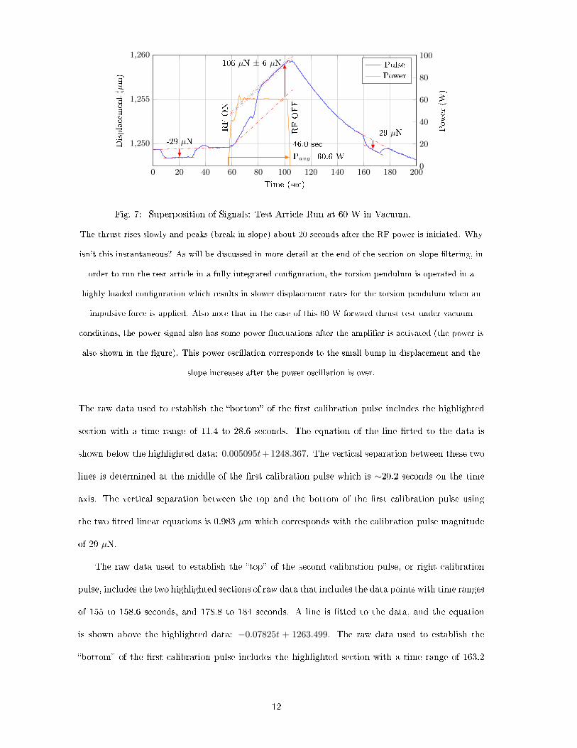
Fig. 7: Superposition of Signals: Test Article Run at 60 W in Vacuum.

The thrust rises slowly and peaks (break in slope) about 20 seconds after the RF power is initiated. Why

isn't this instantaneous? As will be discussed in more detail at the end of the section on slope ltering, in

order to run the test article in a fully integrated conguration, the torsion pendulum is operated in a

highly loaded conguration which results in slower displacement rates for the torsion pendulum when an

impulsive force is applied. Also note that in the case of this 60 W forward thrust test under vacuum

conditions, the power signal also has some power uctuations after the amplier is activated (the power is

also shown in the gure). This power oscillation corresponds to the small bump in displacement and the

slope increases after the power oscillation is over.

The raw data used to establish the bottom of the rst calibration pulse includes the highlighted

section with a time range of 11.4 to 28.6 seconds. The equation of the line tted to the data is

shown below the highlighted data: 0.005095t+ 1248.367. The vertical separation between these two

lines is determined at the middle of the rst calibration pulse which is ∼20.2 seconds on the time

axis. The vertical separation between the top and the bottom of the rst calibration pulse using

the two tted linear equations is 0.983 µm which corresponds with the calibration pulse magnitude

of 29 µN.

The raw data used to establish the top of the second calibration pulse, or right calibration

pulse, includes the two highlighted sections of raw data that includes the data points with time ranges

of 155 to 158.6 seconds, and 178.8 to 184 seconds. A line is tted to the data, and the equation

is shown above the highlighted data: −0.07825t + 1263.499. The raw data used to establish the

bottom of the rst calibration pulse includes the highlighted section with a time range of 163.2

12

to 171.6 seconds. The equation of the line tted to the data is shown below the highlighted data:

−0.0827t + 1263.163. The vertical separation between these two lines is determined at the middle

of the second calibration pulse which is ∼167 seconds on the time axis. The vertical separation

between the top and the bottom of the second calibration pulse using the two tted linear equations

is 1.078 µm which corresponds with the calibration pulse magnitude of 29 µN.

The raw data used to establish the top if the impulsive force from the operation of the test

article includes the highlighted section of raw data in the middle of the plot with a time range of 83.8

to 102.8 seconds. A line is tted to the data and the equation is shown to the left of the highlighted

data: 0.13826t+ 1245.238. The vertical axis intercept (1245.238) to this line is adjusted downward

so that the line that represents the thermally shifted baseline will roughly intersect with the optical

displacement curve where the RF power is turned on. This shifted baseline and its equation is shown

on the plot: 0.13826t+ 1241.468. The vertical shift between the top of the impulsive force and the

shifted baseline is 3.77 µm. The average vertical displacement of the two calibration pulses can be

used to convert this vertical displacement number obtained from the shifted baseline to a force:

F =29µN

0.983µm+1.078µm2

× 3.77µm = 106µN (1)

The tted linear equations are used to generate the dash-dotted lines for the top and bottoms of

the calibration pulses, the top of the impulsive force from the operation of the test article, and the

shifted baseline in Figure 7, Figure 13, and Figure 16.

3. Slope Filtering: Alternate Approach

In the process of developing, applying, and reviewing the signal superposition approach, a

suggestion was provided by reviewers to implement and evaluate slope ltering of the optical dis-

placement data. If the important distinction is that there is a change in slope indicating the presence

of both a thermal and impulsive signal, why not just take the derivative of the displacement sig-

nal and re-plot the curve only showing changes that are greater than a specied level? This has

been done in Figure 9 using an aggressive slope lter level. Comparing the slope-ltered curve to

the co-plotted raw displacement data, the two sections of the curve that are known thermal-only

portions of the curve have been ltered to horizontal in the slope-ltered curve (see time ranges of

13

0 20 40 60 80 100 120 140 160 180 200

1,248

1,250

1,252

1,254

1,256

1,258

1,260

Cal Pulse 1 Top0.004615t+ 1249.360

Cal Pulse 1 Bottom0.005095t+ 1248.367

Force Pulse Top0.13826t+ 1245.238

Shifted Baseline0.13826t+ 1241.468

Cal Pulse 2 Top−0.07825t+ 1263.499

Cal Pulse 2 Bottom−0.0827t+ 1263.163

RFON

RFOFF

Time (sec)

Displacement(µm)

0

20

40

60

80

100

Pow

er(W

)

Pulse

Power

Cal Pulse Top

Cal Pulse Bottom

Force Pulse Top

Fig. 8: Force Measurement Procedure Plot: The gure shows one of the 60W forward thrust runs

with the data annotated to indicate the sections used to determine the calibration pulse

characteristics, and the force pulse characteristics.

∼80-100 seconds, and ∼106-150 seconds). The characteristics of the second calibration curve after

the test run are such that it has a large leading edge and small trailing edge to the pulse. This is a

known impulsive signal that is present while there is also a signicant thermal signal of same sense

(negative-going). The characteristics of the curve while the RF power is applied to the test article

are similar to this calibration pulse which may be an indication that there is an impulsive signal

present with a same-sense thermal signal while the test article is energized. The critical ltered

displacement values for the rst and second calibration pulses and the curve when the RF power is

applied are annotated on the gure, and these values can be used to calculate a force magnitude.

Using the numbers shown to calculate the average displacements for the two calibration pulses and

calculating the average force pulse displacement, the predicted force magnitude using this slope

ltering technique is 124 µN.

One thing that was observed when implementing this approach was that the lter value necessary

to atten the sections of the displacement curve that are known to be thermal-only also resulted

in the reduction in displacement magnitude for the leading calibration pulse, which is known to be

a pure impulsive signal with no background thermal. A possible explanation for this is the fact that

14

0 20 40 60 80 100 120 140 160 180 200

1,250

1,252

1,254

1249.648

1253.624

1253.310

1253.235

1252.288

1252.538

1252.000

1252.462

1252.462

Time (sec)

Slope-ltered

Displacement(µm)

1,248

1,250

1,252

1,254

1,256

1,258

1,260

Raw

Displacement(µm)

Fig. 9: Slope Filtering Plot with aggressive slope lter level.

The solid trace is the ltered data, and the dash-dotted trace is the raw unltered data. The critical

displacement values for the leading calibration pulse, force pulse, and trailing calibration pulse are

annotated on the plot. Using these numbers yields a predicted force magnitude of 124 µN.

the torsion pendulum is highly loaded with mass making the inertial response time to impulsive

forces only slightly faster that the thermal response which means there will be some loss of impulsive

data during aggressive slope ltering. The current implementation with an integrated test article

and all necessary support electronics assembled into a single integral package requires a large amount

of ballast to balance the pendulum arm leaving the torsion pendulum highly loaded. This highly

loaded scenario has made the impulsive response time of the torsion pendulum considerably slower

compared to the response times for previous tests in a split conguration mode.

In the split conguration mode, the amplier and supporting electronics were on the opposite

side of the pendulum from the test article which allowed this equipment to also serve as the ballast

mass cutting the overall mass on the pendulum arm by a factor of two compared to the integrated

approach. Figure 10 shows both ends of the pendulum bar for a split conguration with the test

article on one end, and the support electronics on the other end serving as the ballast. The response

of the pendulum in the split conguration mode to an impulsive signal was considerably faster by

comparison to the current approach. The bottom pane of Figure 10 shows vacuum testing of the

split conguration exciting the TM212 mode at 60 W. The calibration pulses have a magnitude of 29

15

µN. As discussed and can be seen in the data, the inertial response time for this split conguration

is quicker than the integrated approach. Also, the thermal contribution for the split conguration is

smaller in magnitude compared to the impulsive signal, which makes determination of the impulsive

force magnitude an easier aair than the signal superposition approach that is used for the integrated

test article implementation. The physical reason for this reduction in thermal contribution is likely

due to the fact that the amplier was on the back of the pendulum with the ns down and the

amplier on top, so thermal expansion of the aluminum heat sink only moves the amplier mass

up and does not drastically change the CG of the torsion pendulum arm in the horizontal plane.

Future tests with the integrated test article approach will rotate the amplier and heat sink such

that it is in a similar orientation to this historical split conguration testing in an eort to reduce

horizontal CG shift from thermal contributions.

The disadvantage to the split conguration which led to its abandonment was that performing

forward and reverse thrust testing required complete disassembly and reassembly of the RF system

when switching thrust directions which precluded the ability to establish a frozen RF tuning

conguration, and is not compatible with the intention of performing force measurement testing

at another location using another force measurement system. Also, as indicated in Section II B 1,

tuning the thruster to generate optimal thrust is very dicult, and breaking conguration when

switching from forward to reverse thrust was not practical.

4. Force Measurement Uncertainty

The contributors to the force measurement uncertainty are identied and quantied. The con-

version from optical displacement to a force measurement is dependent upon a number of factors.

The calibration force is provided by means of an electrostatic n design (discussed earlier) that

was calibrated oine using a Scientech SA210 precision weighing balance with a measurement un-

certainty of +/-0.0001 g or +/-1 µN. The calibration campaign of the n design evaluated the

performance of the electrostatic combs through a range of n engagement ranging from 10% en-

gaged to 90% engaged. Based on this calibration campaign, the operational n engagement range

was established to be from 30% to 70% which provided roughly 3 mm of operational range, which

16

(a) Test Article (b) Support Electronics (as

ballast)

0 20 40 60 80 100 120 140 160 180 200650

655

660

-29 µN

63 µN

-29 µN

RFON

RFOFF

37.7 secP=60 W

Time (sec)

Displacement(µm)

(c) 60W Forward Thrust Run at Vacuum for Split Conguration

Fig. 10: Split Conguration: The pictures show how the pendulum arm was loaded with the test

article on one end, and the support electronics on the opposite end serving as ballast. The thrust

trace illustrates the quicker rise times for the pendulum in response to an impulsive signal.

is well beyond what was needed for this campaign. The uncertainty in force measurement for this

n-engagement range can be as high as +/-2.2 µN when the ns are at the edges of the operational

range. The calibration voltage is provided by a Fluke 343A DC Voltage Calibrator which has a

voltage uncertainty of +/-0.004 V for a calibration voltage of 200 V which corresponds to a force

uncertainty of +/-0.0005 µN. The optical displacement reading is provided by a Philtec muDMS-

D63 displacement measurement system with a positional uncertainty of +/-0.01 µm when running

in the far mode at 5 samples per second. Based on the magnitudes of the calibration forces used

during the vacuum campaign, this corresponds to a force measurement uncertainty of +/-0.4 µN

(worst case). The seismic contribution to positional uncertainty during vacuum runs was +/-0.05

17

µm which corresponds to a force measurement uncertainty of +/-2.2 µN (worst case). Seismic con-

tributions can be larger in magnitude with a very low frequency on windy days due to waves in

Galveston Bay and the Gulf of Mexico (see green run in Figure 12), but this is operationally con-

trolled by not performing vacuum tests during windy conditions. The placement of the thermally

compensated baseline discussed in the previous section may have some level of uncertainty due to

establishing the intersection point of the shifted baseline and the start of the test. It should be

noted that thermal baseline is assumed to be linear which ts well with observed behaviour. A

conservative value of +/-0.2 µm is applied to this thermal uncertainty which corresponds to a force

measurement uncertainty of +/-4.5 µN (worst case).

The root-sum-square of all of the measurement uncertainties yields a value of 5.6 which means

the overall measurement uncertainty is +/-6 µN. Table 1 provides a tabulation of the measurement

uncertainty contributions and the total measurement uncertainty.

Table 1: Measurement Uncertainty Tabulation

Source Magnitude

SA210 ±1 µN

Fin Calibration ±2.2 µN

Fluke 343A ±0.0005 µN

muDMS-D63 ±0.4 µN

Seismic ±2.2 µN

Thermal ±4.5 µN

Total Error ±6 µN

5. Forward Thrust Overview

The tapered RF test article was mounted on the torsion pendulum as shown in Fig. 11. Forward

thrust is dened as causing displacement to the left in the photo. Viewed from above, the torsion

arm moves clockwise causing the mirror attached to the torsion arm to move away from the optical

displacement sensor, which appears as an upward motion or positive displacement in the plots of

displacement vs. time in Figs. 12 and 13. This displacement is also in the same direction as that

18

due to the CG shift from thermal eects.

Fig. 11: Forward Thrust Mounting Conguration (heat sink is black nned item between test

article and amplier).

A typical data run consists of: 1) a leading calibration pulse, typically either 200 volts or 300

volts equating to 29 µN or 66 µN respectively, that lasts for a few seconds and is released; 2) the

RF system is energized for a period of time ranging from dozens of seconds to well over a minute;

3) an identical trailing calibration pulse. All data is saved digitally, and immediately after the run

photographic evidence of the displays is also taken. During a run, the control and data acquisition

system also records the power forward/reected to/from the test article, and the RF amplier

temperature inside the vacuum chamber. Prior to testing in vacuum, an initial green run (a green

run is dened here as a trial run to conrm proper tuning) is performed at ambient pressure (see

Fig. 12). As discussed earlier in Section IIC 1, the ambient pressure run shows considerably less

thermal shift of the baseline and an almost entirely impulsive thrust pulse that exhibits similar

mN/kW performance as the vacuum impulsive thrust.

The test article was run at 40, 60, and 80 W. Three runs were performed at each power setting

for a total of nine vacuum tests in the forward thrust orientation. Once the system is at vacuum, the

mixture ratio of impulsive signal to thermal baseline signal changes from the ambient in that there

is more thermal baseline shift apparent in the data. Using the analysis techniques discussed in the

Force Measurement Procedure section, the shifting baseline and impulsive signal can be decoupled,

and a magnitude for the impulsive signal found. Figure 13 depicts thrust pulses representative

of each power level used to collect statistical data. Table 2 shows a summary of the detected

19

0 20 40 60 80 100 120 140 160 180 200

1,356

1,358

1,360

-29 µN

54 µN

RFON

RFOFF

33.0 secP=55 W

Time (sec)

Displacement(µm)

Fig. 12: Forward Thrust Green Run, Ambient Pressure Conditions. Error bars are not provided

for green runs.

impulsive thrust from the forward thrust campaign conducted while the test article was under

vacuum conditions (< 8 microtorr).

Table 2: Forward Thrust Results in Vacuum Conditions (µN)

Power Band

40 W 60 W 80 W

Run # Power (W) Force (µN) Power (W) Force (µN) Power (W) Force (µN)

Run 1 40.1 48±6 60.6 106±6 81.3 76±6

Run 2 40.8 30±6 59.7 91±6 83.5 119±6

Run 3 40.8 53±6 61.4 128±6 80.7 117±6

6. Reverse Thrust Overview

The tapered RF test article was mounted on the torsion pendulum as shown in Fig. 14. Reverse

thrust is dened as causing displacement to the right in the photo. Viewed from above, the torsion

arm moves counter-clockwise causing the mirror attached to the torsion arm to move towards the

optical displacement sensor, which appears as a downward motion or negative displacement in the

plots of displacement vs. time in Figs. 15 and 16. As the test article assembly was rotated by 180

degrees, this displacement is also in the same direction as that due to the CG shift from thermal

eects.

20

0 20 40 60 80 100 120 140 160

1,182

1,184

1,186

1,188

RFON

RFOFF

39.8 sec

Pavg=40.8 W

-29 µN -29 µN

30 µN ± 6 µN

Time (sec)

Displacement(µm)

0

20

40

60

80

Pow

er(W

)

Pulse

Power

(a) 40 W

0 20 40 60 80 100 120 140 160 180 200

1,250

1,255

1,260

RFON

RFOFF

46.0 secPavg=60.6 W

-29 µN-29 µN

106 µN ± 6 µN

Time (sec)

Displacement(µm)

0

20

40

60

80

100

Pow

er(W

)

Pulse

Power

(b) 60 W

0 20 40 60 80 100 120 140 160 180

1,195

1,200

1,205

-66µN-66µN

76µN ± 6 µN

RFON

RFOFF

38.3secPavg=81.3W

Time (sec)

Displacement(µm)

0

20

40

60

80

100

Pow

er(W

)

Pulse

Power

(c) 80 W

Fig. 13: Forward Thrust, at Vacuum, Representative Runs. Error bars (± 6 µN) are shown as

black dotted lines.

The three gures show a run at 40 W (top), 60 W (middle), and 80 W (bottom). The power is co-plotted

with the thrust trace. The calibration pulses are annotated based on the analysis of the optical

displacement data. The signal superposition method is used to establish the magnitude of the impulsive

thrust, and the results of the analysis are plotted on each gure.

Aside from pointing direction, the test procedure, power levels, data collection and initial green

21

(a) View from left (b) View from right

Fig. 14: Reverse Thrust Mounting Conguration.

run at atmosphere were performed identically to the forward thrust case. An additional event to

highlight in this reverse thrust eort was that the system tuning was disturbed while transitioning

between the 60 W and 80 W runs (the stub tuner position was moved inadvertently). This required

a re-tuning of the system and a repeat of an ambient pressure green run. Figure 15 shows the

preliminary ambient pressure run performed prior to reverse thrust vacuum testing, and the repeated

ambient pressure run performed after re-tuning the system between the 60 W and 80 W testing.

The test article was run at 40, 60, and 80 W. Three runs were performed at each power setting

for a total of nine tests in vacuum conditions in the reverse thrust orientation. Figure 16 depicts

thrust pulses representative of each power level used to collect statistical data. Table 3 shows a

summary of the detected impulsive thrust from the reverse thrust campaign conducted while the

test article was under vacuum conditions (<8 microtorr).

Table 3: Reverse Thrust Results in Vacuum Conditions (µN)

Power Band

40 W 60 W 80 W

Run # Power (W) Force (µN) Power (W) Force (µN) Power (W) Force (µN)

Run 1 40.9 40±6 60.2 43±6 83.2 74±6

Run 2 41.5 30±6 60.2 83±6 80 71±6

Run 3 41.4 30±6 59.1 67±6 80 69±6

22

0 20 40 60 80 100 120 140 160 180 200

1,072

1,074

1,076

1,078

-29 µN

85 µN

-29 µN

RFON

RFOFF

23 sec

P=60 W

Time (sec)

Displacement(µm)

(a) Ambient Run #1

0 20 40 60 80 100 120 140 160 180 200

1,074

1,076

1,078

1,080

1,082

-66 µN87 µN

-65 µN

RFON

RFOFF

17.4 secP=80 W

Time (sec)

Displacement(µm)

(b) Ambient Run #2

Fig. 15: Reverse Thrust Green Runs, Ambient Pressure Conditions. Error bars are not provided

for green runs.

7. Null Thrust Overview

The tapered RF test article was mounted on the torsion pendulum as shown in Fig. 17. Null

thrust parlance means that the test article is mounted to the torsion pendulum so that its major

thrust axis is parallel to the torsion pendulum beam directed radially inward and unable to aect an

impulsive thrust signal on the pendulum. The CG shift from thermal expansion causes a downward

drift in the optical displacement sensor. This null thrust orientation allows the investigation to

quantify any mundane impulsive thrust signals present associated with the operation of the inte-

grated test article at full RF power. The null thrust testing campaign was undertaken at vacuum

conditions, and there were three runs performed operating the integrated test article up to 80 W, or

equivalent to the maximum power exercised during the forward and reverse thrust tests. Running at

maximum power provides an upper bound on any impulsive systemic contribution to the detected

23

0 20 40 60 80 100 120 140 160 180 2001,030

1,032

1,034- 29 µN - 29 µN

-30 µN ± 6 µN

RFON

RFOFF

23.0 secPavg= 41.4 W

Time (sec)

Displacement(µm)

0

20

40

Pow

er(W

)

Pulse

Power

(a) 40 W

0 20 40 60 80 100 120 140 160 1801,020

1,022

1,024 - 29 µN

- 29 µN

-43 µN ± 6 µN

RFON

RFOFF

22.2 secPavg= 60.2 W

Time (sec)

Displacement(µm)

0

20

40

60

80

100

Pow

er(W

)

Pulse

Power

(b) 60 W

40 60 80 100 120 140 1601,184

1,186

1,188

1,190

1,192

1,194

- 66 µN

- 66 µN

-74 µN ± 6 µN

RFON

RFOFF

41.1 secPavg= 83.2 W

Time (sec)

Displacement(µm)

0

20

40

60

80

100

Pow

er(W

)Pulse

Power

(c) 80 W

Fig. 16: Reverse Thrust, at Vacuum, Representative Runs. Error bars (± 6 µN) are shown as

black dotted lines.

The three gures show a run at 40 W (top), 60 W (middle), and 80 W (bottom). The power is co-plotted

with the thrust trace. The calibration pulses are annotated based on the analysis of the optical

displacement data. The signal superposition method is used to establish the magnitude of the impulsive

thrust, and the results of the analysis are plotted on each gure.

thrust. Figure 18 depicts a representative null thrust test run at 80 W under vacuum conditions.

24

(a) View from end (b) View from side

Fig. 17: Null Thrust Mounting Conguration.

The results from the null thrust testing show no impulsive element in the collected data, only the

thermal signal.

0 100 200 300 400 500 600 700 800 900 1,000

1,188

1,190

1,192

1,194

1,196 - 65.5 µN

- 65.5 µN

RFON

RFOFF

89.4 sec

Time Step (0.2 sec ∆t)

Displacement(µm) Pulse

Fig. 18: Null Thrust Test Run, at Vacuum, 80 W power: Shifting baseline due to thermal, no

impulsive content.

8. Error Sources

A list of possible error sources is provided and discussed:

(a) Air currents possibly generating a false positive signal - the test article is tested in atmo-

spheric conditions and under vacuum conditions. The impulsive thrust performance (mN/kW) was

observed to be nearly the same.

(b) RF interaction with surrounding environment - potential for possible RF patch charging on

walls of vacuum chamber interacting with the test article to cause displacement of torsion pendulum.

Leaking RF elds are kept very low by ensuring RF connections are tight and conrmed by measuring

25

with an RF leakage meter (levels are kept below a cell phone RF leakage level). Any wall interaction

would need to be a well-formed resonance coupling and because of the high frequency would be highly

sensitive to geometry. Keeping the RF test article on resonance inside of the frustum volume requires

a phase locked loop system to maintain resonance as the test article expands during operation, so it

is not likely that the RF test article can establish and maintain an eective external RF resonance.

Testing was performed with the torsion pendulum slid out of the vacuum chamber and an enclosure

was built around the pendulum. While this generated similar force performance to that inside the

chamber, the air currents made the quality of the signal poor. Although RF interaction with the

chamber is not viewed by the investigation team as a likely false positive, a future way to totally

eliminate any concerns would be to test in a larger vacuum chamber.

(c) Magnetic interaction - potential for false positive resulting from DC currents in power cables

interacting during test article operation with ambient magnetic elds (e.g. local earth eld, magnetic

damper) to generate a torque displacement on the pendulum. All DC power cables are twisted pair

or twisted shielded pair to minimize magnetic interaction. The test article is tested in a forward,

reverse, and null thrust orientation, but DC power cable routing and orientation is the same for

all three congurations (power cables come in from the top of the test article) meaning any false

positives would be the same magnitude and polarity for all three tests. This was not observed during

the test campaign.

(d) Thermal - thermal expansion and contraction of items mounted on the torsion pendulum

will shift the CG of the pendulum and result in an oset displacement which can be a false positive.

As was discussed in the section on signal superposition, any false positives from thermal will have a

slower displacement response time on the torsion pendulum when compared to an impulsive thrust

signal similar to the calibration pulse. Further, the test article is mounted to the torsion pendulum

by means of two 1/4 − 20 fasteners at the bottom of the entire assembly, so components of the

test article assembly are free to thermally expand without constraint, resulting in a superposition

of all thermal expansion sources being a curve that is uniformly logarithmic in nature with no

discontinuities of slope. Said another way, since the test article is only constrained by two fasteners

at the bottom, thermal expansion has no mechanical restraints relative to the CG of the torsion

26

pendulum. The integrated thermal signal for the system should be a uniform thermal signal with no

discontinuities. Thus it is reasoned that any discontinuities in slope from the optical displacement

sensor is a strong indicator of the presence of a non-thermal source of displacement. Although

the performance of the impulsive signal under atmospheric and vacuum conditions was nearly the

same, the magnitude of the thermal under vacuum conditions was much larger when compared to

atmospheric conditions. To denitively rule out any residual concerns about thermal error sources,

future test campaigns could employ a test apparatus capable of measuring small torques over much

larger angular displacements. For example, a Cavendish balance approach properly designed to

allow very large rotation angles such as, 90, 180, or even 360 degrees will not be susceptible to this

type of thermal false positive.

(e) Vibration - false positives from vibration are not likely as vibration would not generate a

steady state angular displacement of the torsion pendulum during operation. Contamination of

displacement data from high amplitude vibration is mitigated by the 1.219 m x 2.438 m optical

isolation table, and testing for the record is only performed on days where the ambient vibration

levels still present during testing are of very low magnitudes compared to the displacements from

test activities.

(f) Electrostatic interaction - potential for false positives from charging of moving components

of torsion pendulum relative to stationary components of torsion pendulum and surrounding envi-

ronment. All components of torsion pendulum and surrounding environment are held at a common

reference ground by use of extensive grounding between components. This is conrmed with an

ohm meter.

(g) Outgassing - potential for false positive from vaporization of surface molecules of dielectric

insert or other non-metallic surfaces. During operation, the RF amplier is the warmest component

of the integrated test article. The RF amplier is kept below 90 degrees F for hardware life preserva-

tion, and this temperature is monitored by the supporting lab equipment. Infrared imagery during

operation of the test article shows that the larger end of the cone is the warmest portion of the RF

resonance volume, but less than the amplier. The dielectric is mounted on the smaller end of the

tapered volume. Any outgassing that might occur from the dielectric insert would be vented from

27

the at ends of the cone in an orthogonal, radial axisymmetric manner to the axis of the test article

which would not be detected as a rectied force by the torsion pendulum. Additionally, force from

outgassing being tied to thermal heating would likely have much slower rise and fall times when

compared to the impulsive response from the calibration pulse. Said another way, outgassing would

manifest as a slow increase in displacement (force) when the test article is active, and a similar

slow decrease in displacement (force) back to zero after the test article is shut down and the system

slowly cools down.

(h) Photon rocket - RF leakage from test article generating a net force due to photon emission.

The performance of a photon rocket is several orders of magnitude lower than the observed thrust.

Further, as noted in the above discussion on RF interaction, all leaking elds are managed closely

to result in a high quality RF resonance system. This is not a viable source of the observed thrust.

(i) Uncertainty in impulsive/thermal signal decoupling - Some vacuum thrust traces are unam-

biguous, and decoupling impulsive from thermal is straightforward. In cases where the magnitude

of drift gets very large compared to impulsive, the process is more challenging. One step to improve

any given run is to minimize run time, as that keeps the drift magnitude lower. Another approach

would be to recongure the integrated test article so that the RF heat sink is mounted in such a way

that the thermal expansion is vertical as seen by the pendulum arm whereby minimizing thermal

contamination. As noted earlier, to denitively rule out any residual concerns about thermal error

sources, future test campaigns could employ a test apparatus capable of measuring small torques

over much larger angular displacements.

9. Synopsis of Experimental Results

Figure 19 presents a collection of all the empirically collected data. The averaging of the forward

and reverse thrust data is presented in the form of circles. A linear curve was tted to the data and

is shown with the corresponding tted equation. The vacuum test data collected shows a consistent

performance of 1.2 ± 0.1 mN/kW which is very close to the average impulsive performance measured

in air (also 1.2 mN/kW). The error bars about the average data points represent a 2σ error. The

error bars about the individual data points represents the force measurement uncertainty of ± 6

28

µN.

30 35 40 45 50 55 60 65 70 75 80 85 900

20

40

60

80

100

120

140

160

F = 1.1683P,R2 = 0.746

Power (W )

Force(µN)

Raw Data

Linear Curve Fit

Average Data

Fig. 19: Graph of Forward and Reverse Thrust Vacuum Testing.

10. Discussion

Prior to providing some qualitative thoughts on the proposed physics potentially at work in

the tapered RF test articles, it will be useful to provide some brief background on the supporting

physics lines of thought. In short, the supporting physics model used to derive a force based on

operating conditions in the test article can be categorized as a non-local, hidden-variable theory, or

pilot-wave theory for short.

Pilot wave theories are a family of realist interpretations of quantum mechanics that conjecture

that the statistical nature of the formalism of quantum mechanics is due to an ignorance of an

underlying more fundamental real dynamics, and that microscopic particles follow real trajecto-

ries over time just like larger classical bodies do. The rst pilot wave theory was proposed by de

Broglie in 1923 [4] where he proposed that a particle interacted with an accompanying guiding wave

eld, or pilot wave, and this interaction is responsible for guiding the particle along its trajectory

orthogonal to the surfaces of constant phase. In 1926, Madelung [5] published a hydrodynamic

model of quantum mechanics by recasting the linear Schrödinger equation into hydrodynamic form

29

where the Plank constant h is analogous to a surface tension σ in shallow-water hydrodynamics and

vacuum uctuations are the reason for quantum mechanics. In 1952, Bohm [6, 7] published a pilot

wave theory where the guiding wave is equivalent to the solution of the Schrödinger equation and

a particle's velocity is equivalent to the quantum velocity of probability. Soon after, the Bohmian

mechanics line of thinking was extended by others to incorporate the eects of a stochastic subquan-

tum realm and de Broglie augmented his initial pilot wave theory with this approach in 1964 [8]

adopting the parlance hidden thermodynamics. A family of models categorized as vacuum-based

pilot wave theories or Stochastic Electrodynamics (SED) [9] further explore this idea in that the

zero point eld, electromagnetic vacuum uctuations represent a natural source of stochasticity in

the subquantum realm and provides classical explanations for the origin of the Planck constant,

Casimir eect, ground state of hydrogen, and much more.

It should be noted that the pilot wave domain experienced an early setback when von Neumann

[10] published an impossibility proof against the idea of any hidden-variable theory. This and other

subsequent impossibility proofs were later discredited by Bell 30 years later in 1966 [11], and Bell

goes on to say in the preface of his 1987 book [12] that the pilot wave eliminates the shifty boundary

between wavy quantum states on the one hand, and Bohr's classical terms on the other - said simply

there is a real quantum dynamics underlying the probabilistic nature of quantum mechanics.

While the idea of a pilot wave or realist interpretation of quantum mechanics is not the dominant

view of physics today (which favors the Copenhagen Interpretation), it has seen a strong resurgence

of interest over the last decade based on some experimental work pioneered by Couder and Fort [13].

Couder and Fort discovered that bouncing a millimeter sized droplet on a vibrating shallow uid

bath at just the right resonance frequency created a scenario where the bouncing droplet created a

wave pattern on the shallow bath that also seemed to guide the droplet along its way. To Couder and

Fort, this seemed very similar to the pilot wave concept just discussed, and in subsequent testing by

Couder and others, this macroscopic classical system was able to exhibit characteristics thought to

be restricted to the quantum realm. To date, this hydrodynamic pilot wave analog system has been

able to duplicate the double slit experiment ndings, tunneling, quantized orbits, and numerous

other quantum phenomenon. Bush has put together two thorough review papers chronicling the

30

experimental work being done in this domain by numerous universities[14, 15].

In addition to these quantum analogs, there may already be direct evidence supportive of the

pilot wave approach - specically Bohmian trajectories may have been observed by two separate

experiments working with photons [16, 17]. Reconsidering the double slit experiment with the

pilot wave view, the photon goes through one slit, and the pilot wave goes through both slits.

The resultant trajectory that photons follow are continuous real trajectories that are aected by the

pilot wave's probabilistic interference pattern with itself as it undergoes constructive and destructive

interference due to reections from the slits.

In the approach used in the Quantum Vacuum Plasma Thruster (Q-thruster) supporting physics

models, the Zero Point Field (ZPF) plays the role of the guiding wave in a similar manner to

the vacuum based pilot wave theories. To be specic, the vacuum uctuations (virtual fermions

and virtual photons) serve as the dynamic medium that guides a real particle on its way. Two

recent papers authored by members of this investigation team explored the scientic ramications

of this ZPF-based background medium. The rst paper [18] considered the quantum vacuum at the

cosmological scale in which a thought experiment applied to the Einstein tensor yielded an equation

that related the gravitational constant to the quantity of vacuum energy in the universe implying

that gravity may be viewed as an emergent phenomenon - a long wavelength consequence of the

quantum vacuum. This viewpoint was scaled down to the atomic level to predict the density of the

quantum vacuum in the presence of ordinary matter. This approach yielded a predicted value for

the Bohr radius and electron mass with a direct dependency on dark energy. The corollary from

this work pertinent to the q-thruster models is that the quantum vacuum is a dynamic medium and

can potentially be modeled at the microscopic scale as an electron-positron plasma. The quantum

vacuum around the hydrogen nucleus was considered in much more detail in the second paper[19].

Here, the energy density of the quantum vacuum was shown to theoretically have a 1/r4 dependency

moving away from the hydrogen nucleus (or proton). This 1/r4 dependency was correlated to the

Casimir force suggesting that the energy density in the quantum vacuum is dependent on geometric

constraints and energy densities in electric/magnetic elds. This paper created a quasi-classical

model of the hydrogen atom in COMSOL Multiphysics software (COMSOL is not an acronym)

31

that modeled the vacuum around the proton as an electron-positron plasma. These analysis results

showed that the n = 1 to 7 energy levels of the hydrogen atom could be viewed as longitudinal

resonant acoustic wave modes in the quantum vacuum. This suggests that the idea of treating

the quantum vacuum as a dynamic medium capable of supporting oscillations may be valid. If a

medium is capable of supporting acoustic oscillations, this means that the internal constituents are

capable of interacting and exchanging momentum.

If the vacuum is indeed mutable and degradable as was explored, then it might be possible to

do/extract work on/from the vacuum, and thereby be possible to push o of the quantum vacuum

and preserve the Laws of Conservation of Energy and Conservation of Momentum. It is proposed

that the tapered RF test article pushes o of quantum vacuum uctuations, and the thruster

generates a volumetric body force and moves in one direction while a wake is established in the

quantum vacuum that moves in the other direction.

III. Conclusions

A vacuum test campaign that utilized an updated integrated test article and optimized torsion

pendulum layout has been completed. The test campaign consisted of a forward thrust element

that included performing testing at ambient pressure to establish and conrm good tuning, and

subsequent power scans at 40, 60, and 80 W with three thrust runs performed at each power setting

for a total of nine runs at vacuum. The test campaign consisted of a reverse thrust element that

mirrored the forward thrust element. The test campaign included a null thrust test eort of three

tests performed at vacuum at 80W to try and identify any mundane sources of impulsive thrust; none

were identied. Thrust data from forward, reverse, and null suggests that the system is consistently

performing at 1.2 ± 0.1 mN/kW which is very close to the average impulsive performance measured

in air. A number of error sources were considered and discussed. While thermal shift was addressed

to a degree with this test campaign, future testing eorts should seek to develop testing approaches

that are immune to CG shifts from thermal expansion. As indicated in the error section, a modied

Cavendish balance approach could be employed to denitively rule out thermal. Although this test

campaign was not focused on optimizing performance and was more an exercise in existence proof,

32

it is still useful to put the observed thrust to power gure of 1.2 mN/kW in context. The current

state of the art thrust to power for a Hall thruster is on the order of 60 mN/kW. This is an order

of magnitude higher than the test article evaluated during the course of this vacuum campaign,

however, for missions with very large delta-v requirements, having a propellant consumption rate

of zero could oset the higher power requirements. The 1.2 mN/kW performance parameter is

over two orders of magnitude higher than other forms of zero-propellant propulsion such as light

sails, laser propulsion, and photon rockets having thrust to power levels in the 3.33-6.67 µN/kW (or

0.0033-0.0067 mN/kW) range.

Acknowledgments

The primary author would like to thank the Eagleworks team for support and hearty discussions

about the concepts and testing discussed and explored in this paper. The primary author would

also like to thank Andrew Chap for detailed and rigorous work to validate and optimize the plasma

analysis tools. The team would like to thank the National Aeronautics and Space Administration

for organizational and institutional support in the exploration and analysis of the physics in this

paper.

References

[1] Brady, D., White, H., March, P., Lawrence, J., and Davies, F., Anomalous Thrust Production from an

RF Test Device Measured on a Low-Thrust Torsion Pendulum, 50th AIAA/ASME/SAE/ASEE Joint

Propulsion Conference, AIAA 2014-4029, AIAA, Jul. 2014. doi:10.2514/6.2014-4029

[2] Tajmar, M., and Fiedler, G., Direct Thrust Measurements of an EMDrive and Evaluation of Possible

Side-Eects, 51st AIAA/ASME/SAE/ASEE Joint Propulsion Conference, AIAA 2015-4083, AIAA,

Jul. 2015. doi:10.2514/6.2015-4083

[3] Yan, A., Appel, B., Gedrimas, J., MilliNewton Thrust Stand Calibration Using Electrostatic Fins,

47th AIAA Aerospace Sciences Meeting including The New Horizons Forum and Aerospace Exposition,

AIAA, Jan. 2009. doi:10.2514/6.2009-212

[4] de Broglie, L., Interpretation of quantum mechanics by the double solution theory, Annales de la

Fondation Louis de Broglie, Vol. 12, No. 4, 1987, pp. 1-23.

33

[5] Madelung, E., Quantentheorie in hydrodynamischer Form, Zeitschrift für Physik A Hadrons and

Nuclei, Vol. 40, Issue 3, 1927, pp. 322-326. doi:10.1007/BF01400372

[6] Bohm, D., A Suggested Interpretation of the Quantum Theory in Terms of Hidden Variables. I,

Phys. Rev., Vol. 85, Issue 2, 1952, pp.166-179. doi:10.1103/PhysRev.85.166

[7] Bohm, D., A Suggested Interpretation of the Quantum Theory in Terms of Hidden Variables. II,

Phys. Rev., Vol. 85, Issue 2, 1952, pp.180-193. doi:10.1103/PhysRev.85.180

[8] de Broglie, L., La thermodynamiquecachée des particules, Annales de l'I.H.P. Physique théorique,

Vol. 1, No. 1, 1964, pp.1-19.

[9] Boyer, T. H., Any classical description of nature requires classical electromagnetic zero-point radiation,

American Journal of Physics, Vol. 79, No. 11, 2011, pp. 1163-1167. doi:10.1119/1.3630939

[10] von Neumann, J., Mathematische Grundlagen der Quantenmechanik (Springer, Berlin 1932).

[11] Bell, J. S., On the Problem of Hidden Variables in Quantum Mechanics, Reviews of Modern Physics,

Vol. 38, Issue 3, 1966, pp.447-452. doi:10.1103/RevModPhys.38.447

[12] Bell, J. S., Speakable and Unspeakable in Quantum Mechanics (Cambridge Univ. Press, Cambridge, UK

1987).

[13] Couder, Y., Fort, E., Single-Particle Diraction and Interference at a Macroscopic Scale, Physical

Review Letters, Vol. 97, Issue 15, 2006, pp.154101. doi:10.1103/PhysRevLett.97.154101

[14] Bush, J. W. M., The new wave of pilot-wave theory, Physics Today, Vol. 68, 2015, pp. 47-53.

doi:10.1063/PT.3.2882

[15] Bush, J. W. M., Pilot-wave hydrodynamics, Annual Review of Fluid Mechanics, Vol. 47, 2015, pp.

269-292. doi:10.1146/annurev-uid-010814-014506

[16] Kocsis, S., et. al., Observing the Average Trajectories of Single Photons in a Two-Slit Interferometer,

Science, Vol. 332, Issue 6034, 2011, pp.1170-1173. doi:10.1126/science.1202218

[17] Mahler, D. H., et. al., Experimental nonlocal and surreal Bohmian trajectories, Science Advances,

Vol. 2, Issue 2, 2016, e1501466. doi:10.1126/science.1501466

[18] White, H., A Discussion on Characteristics of the Quantum Vacuum, Physics Essays, Vol. 28, No. 4,

2015.

[19] White, H., Vera, J., Bailey, P., March, P., Lawrence, T., Sylvester, A., and Brady, D., Dynamics of

the Vacuum and Casimir Analogs to the Hydrogen Atom, Journal of Modern Physics, Vol. 6, 2015,

pp.1308-1320. doi: 10.4236/jmp.2015.69136

34