Measurement of the Lidar Ratio for Atmospheric Aerosols using a

180°-Backscatter Nephelometer

Doherty, Sarah J.

Department of Atmospheric Sciences, University of Washington, Box 351640, Seattle, WA

98195-1640

Anderson, Theodore L.

Joint Institute for the Study of the Atmosphere and Oceans, University of Washington, Box

351640, Seattle, WA 98195-1640

Charlson, Robert J.

Department of Atmospheric Sciences, University of Washington, Box 351640, Seattle, WA

98195-1640

Applied Optics: Lasers, Photonics, and Environmental Optics

Doherty, S.J., T.L. Anderson, and R.J. Charlson, Measurement of thelidar ratio for atmospheric aerosols with a 180degree backscatternephelometer, Applied Optics, 38(9), 20 March 1999, 1823-1832.

1

Abstract:

Laser radar (lidar) can be used to estimate atmospheric extinction coefficients due to

aerosols if the ratio between optical extinction and 180° backscatter (the "lidar ratio") at the laser

wavelength is known or if Raman or high spectral resolution (HSR) data is available. Most lidar

instruments do not have Raman or HSR capability, however, making knowledge of the lidar ratio

essential. We have modified an integrating nephelometer, which measures the scattering

component of light extinction, by addition of a backward pointing laser light source such that the

detected light corresponds to integrated scattering over 176°-178° at a common lidar wavelength

of 532 nm. Mie calculations indicate that the detected quantity is an excellent proxy for 180°

backscatter. When combined with existing techniques for measuring total scattering and

absorption by particles, the new device permits a direct determination of the lidar ratio. A four-

point calibration, run by filling the enclosed sample volume with particle-free gases of known

scattering coefficient, indicates a linear response and calibration reproducibility to within 4%. The

instrument has a detection limit of 1.5x10-7 m-1 sr-1 (~10% of Rayleigh scattering by air at STP)

for a 5 minute average, and is suitable for ground and mobile/airborne surveys. Initial field

measurements yielded a lidar ratio of ~20 for marine aerosols and ~60-70 for continental aerosols,

with an uncertainty of ~20%.

Key words: lidar ratio, nephelometer, backscatter, climate forcing, aerosol, light scattering

2

1.0 Introduction

A recent National Research Council panel report1 summarizes six independent lines of

evidence supporting the hypothesis that direct (i.e. clear-sky) climate forcing due to the scattering

and absorption of sunlight by anthropogenic aerosols is a major factor in global climate change.

Visibility is similarly known to depend on scattering and absorption of light by atmospheric

aerosols. A variety of aerosol measurements (as well as theoretical models) contribute to this

evidence, but notably lacking is a physically meaningful contribution from elastically scattering

lidar. Nevertheless, the potential contribution of this technology is enormous, given its exquisite

precision, vertical resolution, and the relative ease of data acquisition. This potential has yet to be

exploited because of difficulties in quantitatively and accurately relating the elastically scattered

lidar signal to the aerosol parameters relevant to climate forcing and visibility.

Analogous to radar but operating at shorter wavelengths, a lidar instrument transmits

pulsed laser radiation and measures what is backscattered by gases, particles, or other objects in

the atmosphere. The return time of the signal corresponds to distance from the transmitter such

that range-dependent information is acquired. The intensity of the signal depends on two

quantities: (1) how effectively the laser radiation is backscattered at a specific location in the

atmosphere and (2) how effectively the laser radiation is extinguished by the intervening

atmosphere. Interpreting the lidar signal depends on an ability to separate these two quantities -

local 180° backscatter and optical depth over the entire range. It is this deconvolution of local

backscatter and range-dependent optical depth which is at the heart of the lidar retrieval

challenge.

Following instrument calibration2, a vertically-pointing lidar provides a direct measurement

of the quantity S(z):

S(z) = Aβ(z)exp[− 2 σezLz∫ (z' )dz] = Aβ(z)exp[ − 2τ(zL,z)] (1)

where A is an instrumental calibration constant, β(z) is the 180° backscatter coefficient (m-1 sr-1)

from both molecules and aerosols at height z (m), σe is the extinction coefficient (m-1) from both

3

molecules and aerosols at height z, and τ(zL,z) is the extinction optical depth between the lidar

height, zL, and z. Eq. 1 shows that the fundamental challenge of converting the lidar

measurement, S(z), to a geophysically meaningful aerosol quantity is to disentangle β and τ - or,

equivalently, β and σe. Since molecular scattering can be predicted accurately from air density

(i.e. temperature and pressure) information, this challenge reduces to disentangling particulate

backscattering, βp, from particulate extinction, σep. Two types of technologically advanced lidar

systems, Raman lidar and high spectral resolution lidar, are able to separate these terms by making

auxiliary measurements of the return signal. These instruments are described briefly in Section 4.

For lidar systems that detect elastically scattered light only, the quantities βp and σep can be

disentangled if the ratio of the two parameters is known. This quantity is referred to as the lidar

ratio3, K,

K(sr ) =σep

βp=

σsp + σap

βp(2)

where σsp and σap are the components of particulate extinction due to light scattering and light

absorption, respectively.

Based on Mie calculations that incorporate the ranges of particle size distributions and

refractive indices encountered in the troposphere, possible values of K span at least an order of

magnitude, from approximately 10 to 100 ( sr). The lower values correspond to coarse-particle

aerosols like soil dust and sea salt, while the higher values represent fine particles of smoke and

products of gas-to-particle conversion. To explore the sensitivity of lidar-retrieved optical depth

to uncertainties in K, we use data from the recent lidar demonstration Shuttle mission4 (LITE).

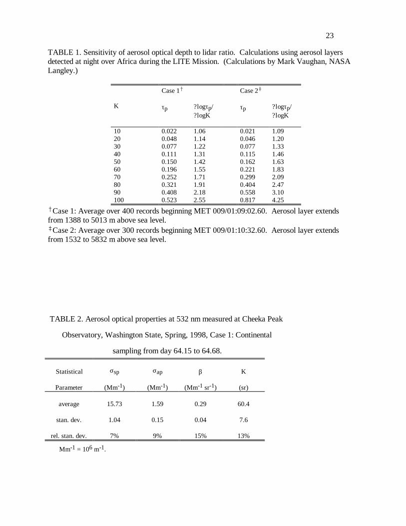
Table 1 shows the effect on retrieved optical depth of allowing K to vary from 10 to 100. Data

consists of two cases when aerosol layers were detected at night over Africa during the LITE

mission. The columns labeled ?logτp/?logK indicate how a fractional uncertainty in lidar ratio

would translate into a fractional uncertainty in optical depth. This sensitivity parameter is seen to

vary between the two cases and to be a strong function of lidar ratio. For low K values, K and τp

are nearly proportional. For the higher K values (which tend to be characteristic of pollution-

4

derived particles in the sub-µm size range), the sensitivity is considerably higher - up to a factor of

4. Overall, the factor of ten range of possible lidar ratios translates into a factor of 10 to 40

uncertainty in retrieved optical depth. This range is too large to offer an adequate constraint on

lidar retrievals for the problems of climate forcing or visibility.

For lack of accurate knowledge of K, most aerosol measurements by elastically scattered

lidar are reported as a "scattering ratio" - that is, the ratio of the calibrated signal to the expected

signal for particle-free air.5-12. This is useful for qualitative identification of aerosol layers, but

not for input into radiative transfer models. The instrument described herein provides a relatively

inexpensive method for accurate local measurement of βp. When combined with existing

instrumentation for measuring σep, this permits an empirical determination of K.

Being small and portable, the new device permits routine ground-based monitoring as well as

airborne surveys of βp and K, which will, in turn, allow extensive lidar data sets on tropospheric

aerosols to be applied in a quantitative fashion to the aerosol/climate and visibility problems.

2.0 Design Details

Two technical developments combined to make the 180° nephelometer feasible. First is the

commercial development and laboratory validation13 of a high-sensitivity integrating

nephelometer (TSI, Inc., St. Paul, MN). This instrument performs a geometrical integration of

the angular distribution of scattered intensity such that the scattering coefficient of a gaseous or

aerosol medium can be measured with the combination of a Lambertian light source and an

orthogonal light detector. Two versions of the nephelometer are currently available: the 3551,

which measures light scattering at one wavelength (550nm) and the 3563, which measures

scattering at three wavelengths (450, 550, and 750nm). The instrument already incorporates

several key design features needed for accurate measurement of βp.

1) The scattering volume is enclosed, allowing calibration with gases of known

scattering coefficient. Scattering by particle-free air can be measured and

5

subtracted from subsequent measurements of air containing aerosol to derive light

scattering due to particles only, σsp.

2) A reference chopper is used to alternate between measurement of dark counts, the

scattering signal, and a reference signal. The system signal thus is corrected for

dark count, changes in lamp brightness, and changes in photomultiplier tube

sensitivity using the dark and reference signals.

3) The temperature and pressure within the sensing volume are continuously

monitored, so the amount of scattering coming from air within the sensing volume

can be accurately calculated and subtracted from total scattering to determine

scattering due to particles only (σsp).

The second technological development of import is the commercial production of a diode-

pumped laser operating at 532nm (Uniphase 10mW Microgreen laser). This laser is more

compact and stable than gas lasers operating at similar wavelengths and can be incorporated into

the TSI nephelometer to provide an alternate, single-beam source of illumination.

Figure 1 schematically shows how a basic version of the integrating nephelometer (model

3551) has been modified to measure near-180° backscatter. The laser and associated optics are

added to produce a collimated beam of light that is aimed very nearly along the optical axis of the

nephelometer sample volume, pointing away from the detector. With this arrangement, light

reaching the detector has either been scattered at near-180° by molecules and particles in the

sample volume or it has been scattered off the interior walls. Variations in the laser intensity and

detector sensitivity are continuously monitored via a reference beam (Figure 2). Mie calculations

show that the 176°-178° scattering integral actually sensed by the nephelometer is an excellent

proxy for 180° backscatter for a broad range of particle size distributions and refractive indices

(Figure 3). Periodic calibration with gases determines wall scattering (to be subtracted) and the

factor that converts the remaining signal to β.

6

As designed, the system can be run both as a 180° nephelometer, using the laser as the light

source, or as a normal nephelometer, using the built-in tungsten-halogen lamp. Ideally,

electronically controlled shutters would be integrated into the system for rapid, automatic

switching between the two modes, although manual switching between light sources is possible

with the current design. In either case, for a valid comparison of total scatter to 180°-backscatter

an assumption would need to be made about the stability of the sampled aerosol with time. For

the field data presented herein (Section 5), the three quantities needed to determine K (σsp, βp,

and σap) were measured simultaneously with separate instruments.

3.0 Gas calibration & noise measurements

As a closed-volume device, the 180° nephelometer is calibrated with gases of known

backscattering coefficient. These absolute calibrations can be performed routinely in the field to

maintain a record of calibration stability and an analysis of instrumental noise. In this way,

detection limits are quantified and performance is continuously monitored. The system can also

be calibrated with monodisperse, laboratory generated particles, where the measured 180°

backscatter would be compared to calculated values using Mie theory, as has been done for the

integrating nephelometer13.

The basic algorithm for deriving βp from the measured photon counts is:

βp = k2 C − Cwall( )− βair(T,P) (3)

where k2 is the calibration slope, C (the instrument signal) is the normalized photon counting rate

measured by photo-multiplier tube (PMT), Cwall is the calibration offset, which can be interpreted

as photon counts associated with scattering off the inside walls, and βair is the calculated 180°

backscatter coefficient of air at the temperature (T) and pressure (P) measured inside the

instrument. The normalized photon counts, C, are corrected for dark counts (Cdark) and

variations in laser brightness and PMT sensitivity (via changes in Ccal):

C =Cmeas − Cdark( )Ccal − Cdark( ) (4)

7

A rotating shutter alternately exposes the PMT to backscattered photons, no photons, and a small

portion of the laser beam itself to determine Cmeas, Cdark, and Ccal, respectively.

The backscattering coefficient of the calibration gases is known to be a function of the

refractive index and the molecular anisotropy of the gas14,15 as follows:

βgas(λ) = σsg(STP,λ)3

8π(1 + γ)

(1 + 2γ)273.2

TP

1013.2(5)

where σsg (STP,λ) ) is the scattering coefficient at standard temperature and pressure for a given

wavelength, γ is a factor accounting for molecular anisotropy, T is the temperature in K, and P is

the pressure in hPa. All required parameters are most accurately known for dry air and CO2;

thus, these are the calibration gases of choice for most nephelometer applications16, including our

own. For air and CO2, at 532nm σsg(STP)-values are 1.3888x10-5 and 3.5969x10-5 (m-1),

respectively, and γ-values are 0.01442 and 0.04325, respectively.15,17 Thus, βair(STP) is

1.63x10-6 (m-1 sr-1) and βCO2(STP) is 4.12x10-6 (m-1 sr-1). Given knowledge of the calibration

gases, the calibration constants are determined as:

k2 =βCO2 − βair( )CCO2 − Cair( ) Cwall = Cair − βair

k 2(6)

Note that CCO2 and Cair are actually measured over the angular range 176°-178°, where as the

known values, βCO2 and βair, are for a 180° scattering angle. Implicit in k2, then, is the

conversion from σgas,176°-178° to βgas. This conversion is carried over with k2 to all other

scattering measurements.

We have performed a 4-point calibration (using air and CO2 at pressures of 1 and 0.5 atm) of

the 180° nephelometer which indicates excellent linearity (Figure 4) and very small wall

scattering. (Cwall is less than 5% of C for particle-free air.) In addition, we have performed

numerous measurements of air and CO2 to study noise levels, mechanical stability, sensitivity to

laser beam alignment, etc. These tests yielded calibration constants that varied by <4% under

normal working conditions and indicated a detection limit for 5-minute averages of approximately

0.10 times βair.

8

4.0 Relation to previous instruments and approaches

A. The backscattersonde

The "backscattersonde" described by Rosen and Kjome18 is similar to our 180°

nephelometer in that it offers a local measurement of βp. It is light and inexpensive, and thus

well-suited for balloon-borne measurements of atmospheric backscatter versus altitude; in

contrast, the instrument described herein is currently both too large and too expensive for routine

balloon deployment. The backscattersonde has been used to determine the lidar ratio by running

it in parallel with a separate instrument that measures scattering and with assumptions about

particle absorption.19-21

The backscattersonde has an open sensing volume and a flashlamp light source, so it cannot

be calibrated in the laboratory with gases or with particles of known concentration, size and

refractive index, and it can only be used at night. The present calibrations rely on measurements

of air Rayleigh backscattering in the stratosphere in the winter Arctic polar vortex, where particle

concentrations are believed to be insignificant. Previous or subsequent measurements in other

regions rely on inter-instrument calibration via comparison to reference instruments. However,

optical and electronic components may be subject to drift and the resulting uncertainty has not

been determined. The instrument senses backscattering over a broad angular range (~160°-179°)

and over two broad wavelength ranges centered at 490 and 700 nm, with bandwidths of about

100 nm. The backscatter at 532 nm is derived by linear interpolation. For these reasons, even for

a calibrated system, converting the measured quantity to βp at 532 nm would require an optical

model of the instrument and Mie calculations based on assumptions about particle size, refractive

index, and sphericity. Thus, the backscattersonde offers a proxy for βp at 532nm that requires

calculations and assumptions not required by our 180° nephelometer.

B. Raman lidar & High Spectral Resolution Lidar (HSRL)

Another technique related to the one presented herein is the Raman lidar method.22-29

Molecular and aerosol contributions to light extinction are separated in this method by measuring

9

Raman-shifted laser light at the appropriate wavelengths for nitrogen, oxygen, carbon dioxide

and/or water vapor. Laser light that has been elastically scattered by both molecules and aerosols

is also measured. The intensity of the Raman-shifted backscatter from a given altitude depends on

σsg(z), σsp(z), and on βgas(z), but not on βp(z). The terms σsg(z) and βgas(z) can be calculated,

given an assumed or measured (with a radiosonde) atmospheric density, so inversion yields σsp(z)

at the Raman-shifted wavelength. Aerosol extinction at the original laser wavelength is

determined from the Raman-shifted signal by using an assumed wavelength-dependence of light

scattering, which is based on an assumed size distribution.

To date, this technique has mostly been applied to ultra-violet wavelengths. Because of the

strong wavelength dependence of the lidar ratio (according to Mie calculations) for particles

below about 10 µm, lidar ratios measured at UV wavelengths with Raman lidar are not directly

applicable to visible-wavelength lidar. Conversion to visible wavelengths requires use of an

aerosol model (essentially, an assumed aerosol size distribution) that can introduce uncertainties

of a factor of two.

High spectral resolution lidar (HSRL), like Raman lidar, solves the lidar inversion problem

by separating the backscattered light into particulate and molecular components.30-33 HSRL

takes advantage of the fact that molecules in the atmosphere have much greater Brownian motion

than particles, so backscattered light from molecules is wavelength-broadened around the original

laser wavelength. An interferometer is used to measure this broadened molecular backscatter. As

with the Raman-shifted backscatter described above, the molecular return signal depends on total

extinction and gaseous backscatter only, so σsg(z) can be determined directly, given σsg(z) and

βgas(z).

Both the Raman lidar and HSRL are quite expensive and technologically complex. Like

other remote or open-air devices (including the backscattersonde), they cannot be calibrated with

laboratory particles of known optical properties, such that the absolute accuracy of their inversion

is difficult to quantify. Independent verification of the measured optical properties is therefore

useful. On the other hand, these open-air devices have the enormous advantage of measuring the

10

undisturbed ambient aerosol and can be used to explore vertical variations in the lidar ratio and its

sensitivity to ambient relative humidity.

C. Calibration approaches for lidars with elastic backscatter only

Retrieval of aerosol optical parameters from lidar systems without Raman capability is also

possible, given certain assumptions and/or coincident measurements by other instruments.

Sunphotometers are often used to measure total column optical depth (τ) for vertically pointing

lidars.34-37 Generally, τ must be wavelength corrected to the given lidar wavelength. In addition,

τ is measured for the entire atmosphere, whereas the lidar measurement is only over a portion of

the atmosphere (zL-z in Eqn. 1). One approach is to assume that above z the atmosphere is

aerosol-free and use a fixed lidar ratio to determine aerosol extinction from the lidar and

sunphotometer data alone.34 Takamura et al.35,36 used the sunphotometer in conjunction with an

optical particle counter (OPC), which determines the ground-level aerosol size distribution for an

assumed index of refraction. They calculated aerosol extinction and backscatter - and thus the

lidar ratio - from Mie theory and the OPC data. Aerosol optical properties were considered to be

horizontally and vertically homogeneous. They assumed the return signal from the stratosphere

was aerosol-free and so used it for lidar absolute calibration. As the authors point out, this

approach is invalid after significant volcanic eruptions, such as of Mt. Pinatubo in June, 1991.

Hayasaka et al.37 took a similar approach to Takamura et al., but instead of using an OPC

they used an aureolemeter, which views forward-scattered sunlight. The instrument gives a

columnar averaged size distribution, assuming spherical aerosols with a given index of refraction;

this information is useful for Mie calculations of aerosol scattering. An advantage of this method

is that forward-scattered radiation is not as sensitive to shape and index of refraction as it is to

size, so error in the assumed input parameters is not likely to significantly corrupt the derived size

distribution.

Bistatic lidars measure scattered light at a range of angles, providing information on the

phase function of the column-averaged aerosol. This data can be used to determine the most

probable aerosol index of refraction and size distribution.38,39 Mie calculations are then

11

employed to perform the lidar inversion. Hoff et al.12 used a ground-based nephelometer with a

vertically-pointing lidar and calculated lidar ratios by assuming no light absorption and vertical

homogeneity. Yang et al.40 made no auxiliary measurements, using Mie theory with an assumed

aerosol size distribution and refractive indices from D'Almeida et al.41 Lidar ratios calculated

from their retrieved data are unrealistically low (2 to 7), leading us to conclude that either their

method or the data from D'Almeida et al. is erroneous.

Several groups have made measurements of aerosol optical properties in the boundary layer

using horizontally pointing lidars.42-44 This is a somewhat easier retrieval problem, in that

assumptions of aerosol homogeneity over the lidar optical path are more likely to be accurate.

Jorgensen et al.42 used a hard target with fixed optical properties to calibrate their lidar, then

derived aerosol optical properties for a generated smoke cloud of high optical depth. Young et

al.43 used meteorological data from the lidar site to calculate molecular scattering and an Active

Scattering Aerosol Spectrometer Probe (ASASP) to determine the aerosol size distribution at the

site. In horizontally homogeneous conditions (i.e., when the lidar signal decreased linearly with

range), the lidar ratio could be derived from this data alone. Zhang and Hu44 used filter sampling

methods and an optical particle counter to determine aerosol size and refractive index, then

calculated lidar ratios using Mie theory. Assuming horizontal homogeneity, the system calibration

was complete.

All of these approaches to lidar data retrieval require some combination of additional

measurements and assumptions about the physical properties of the aerosols. Mie theory is

almost always employed to connect these properties to light scattering characteristics, which must

be known to retrieve physically meaningful data from the lidar signal. However, Mie theory may

inaccurately represent the optical properties of the aerosols, especially if they are non-spherical,

even if the input parameters are correct. Direct determination of aerosol's lidar ratio eliminates

the need for measurements and assumptions about particle physical properties and subsequent

calculation of optical properties.

12

5.0 Lidar ratio measurements

Field measurements of the lidar ratio, K (Eq. 2) were made at Cheeka Peak Observatory

(CPO), located at 480m altitude in the far northwest corner of Washington state. This coastal

station samples a wide variety of airmass types, including clean marine air (the dominant

category), continental air affected by urban/industrial pollution in the Pacific Northwest, and

occasionally, polluted air from Asia. Three optical quantities, σsp, σap, and βp, were measured to

calculate K. The first two, which determine σep, were measured with existing instrumentation.

Scattering was measured using an integrating nephelometer (TSI model 3563) and σap by an

absorption photometer that responds to differential transmission of light through a filter (model

PSAP, Radiance Research, Seattle, WA.) All quantities were measured at low relative humidity

(RH < 40%). Impactors were used to alternate every 5 minutes between measuring aerosol with

diameter D=10µm and aerosol with D=1µm, so both fine and coarse mode data were acquired.

Several adjustments to the nephelometer and absorption photometer measurements were

necessary for accurate determination of K. We corrected for angular non-idealities in the

nephelometer measurement of σsp using the procedure described by Anderson and Ogren16. For

the absorption photometer, we used the calibration and scattering correction recommended by

Bond et al.45. Finally, both scattering and absorption were measured at 550 nm wavelength and

were adjusted to the 532 nm laser wavelength using a power law relationship as defined by the

ångström exponent, å:

å λ1 λ2( )= −log σsp

λ1 σspλ2( )

log λ1 λ2( ) (7)

The value of å was empirically determined for σsp by using the 3-wavelength nephelometer

scattering measurements at 550 and 450 nm. For conversion of σap from 550 to 532 nm, å was

assumed to be 1.0. The combined effect of these adjustments is to increase light extinction, σep,

by up to 40% relative to its uncorrected value, primarily due to the correction of the integrating

nephelometer for truncation errors for coarse particles16,45. Following these adjustments, the

uncertainty in σep is less than 20% for the Cheeka Peak data set. These corrections are more

13

important for the coarse particle aerosols (e.g. dust, sea salt) and less important for fine particles

(e.g. industrial pollution).

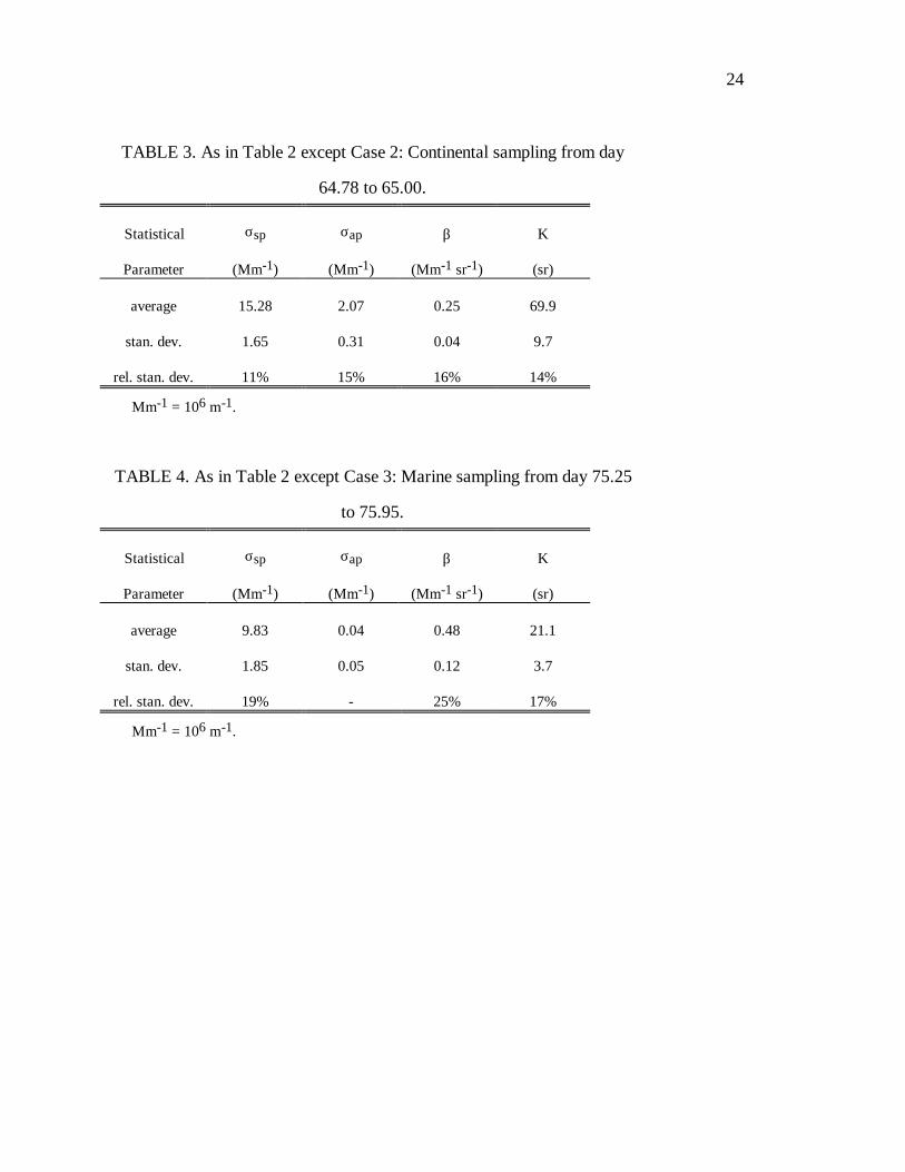
Aerosol optical properties during two distinct sampling periods, one continental and one

marine, are presented in Tables 2-4 and Figures 5 & 6. The continental data are separated into

two cases (Tables 2 & 3) to reflect a step-change in aerosol light absorption (see Figure 5d). Our

measurement protocol involved separate analysis of sub-1 µm and sub-10 µm diameter particles.

Here we present only the sub-10 µm measurements; however, analysis of the complete data set

reveals that the continental aerosol is dominated by sub-µm particles while the marine aerosol is

dominated by super-µm particles. This is confirmed by the contrasting values of å - around two

for the continental period (Figure 5e) and zero for the marine period (Figure 6e). The continental

aerosol has a significant absorption component, indicative of pollution, whereas the marine

aerosol is non-absorbing, consistent with seasalt composition.

The fine-mode dominated continental air has a much higher lidar ratio that the coarse-mode

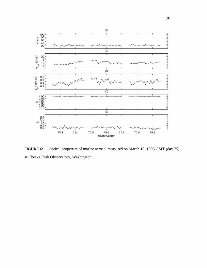
dominated marine air, as is consistent with Mie theory. For the marine case, the lidar ratio is

relatively constant, despite large changes in total aerosol amount (as reflected by changes in total

extinction, Figure 6b). In all three cases, the variability in the lidar ratio is ~15%, which we

attribute to instrumental noise rather than to real variation in the ambient aerosol lidar ratio. The

180° nephelometer laser stability degraded during the field campaign, significantly affecting the

instrument performance. The data presented herein are from times when the laser was relatively

well-behaved. Clean air measurements were used to correct for offset variation, and span gas

calibrations were made in close proximity to each sample period. Based on this information, we

estimate that the lidar ratios presented herein are accurate to within 20%. We expect to improve

the uncertainty in our measurements when the instrument is run with a laser which conforms to

the manufacturer stability specification of <1% variation. Still better results should be possible

with higher aerosol loads via higher signal-to-noise ratios.

14

6.0 Conclusions and future work

The 180° nephelometer presented herein, when used with a total-scatter nephelometer and an

instrument that measures light absorption, allows for empirical determination of βp and the lidar

ratio, obviating the need to rely exclusively on values calculated from Mie theory. Such

calculations not only involve uncertainties associated with input size distributions and refractive

indices but also rely on assumptions of particle homogeneity and sphericity. The instrument is

suitable for routine ground-based monitoring as well as periodic airborne surveys of βp and K.

The closed-cell design of the 180° nephelometer permits an absolute calibration with gases;

therefore, βp can be determined without assumptions about particle shape, composition, or state

of mixture.

Initial field results show a sharp contrast between the lidar ratio of polluted continental

aerosol (60-70) and clean marine aerosol (~20). Uncertainties in these values are on the order of

20%, largely due to instrumental noise in the 180° nephelometer. This noise has been traced to

low photon counting rates for the reference beam and to erratic behavior of the laser during the

field deployment.

Minor changes to the optical arrangement are being implemented to increase the reference

beam intensity. Following the methods described by Anderson et al.14 for the integrating

nephelometer, we will validate the measurement of particulate backscatter using laboratory

generated monodisperse latex spheres of known βp.

Further enhancements to the nephelometer could be undertaken. The current design allows

for measurement of both βp and σsp with a single instrument, via manual switching between the

laser and nephelometer lamp light sources. However, shutters synchronized with the reference

beam chopper could be placed in front of the laser and the lamp, allowing nearly simultaneous

measurement of the two quantities, βp and σsp.

Shape effects may be a dominant source of uncertainty in theoretical determinations of the

lidar ratio, especially for coarse mode dust and seasalt particles. Our empirical method of

determining the lidar ratio could be used to study shape effects and would be enhanced in this

15

regard by adding a polarization measurement. At present, the instrument measures the sum of

polarized plus depolarized scattered light. A second detection channel could be added to measure

only the depolarized scattered light. The ratio of these two quantities (the depolarization ratio)

should be a sensitive indicator of non-sphericity. Modifications to this end are being pursued.

Acknowledgments: This work was supported by the National Aeronautics and Space

Administration (grant #NAG 1 1877) with additional support provided by the National Science

Foundation (grant #ATM-9320871), and by the National Oceanic and Atmospheric

Administration (Joint Institute for the Study of the Atmosphere and Ocean (JISAO) agreement

#NA37RJ0198, contribution #575). We would also like to thank Steven Domonkos of the

University of Washington Dept. of Atmospheric Sciences for his invaluable contributions to the

deign and construction of the instrument.

16

References and Notes

1. J. H. Seinfeld, R. J. Charlson, P. A. Durkee, D. Hegg, B. J. Huebert, J. Kiehl, M. P.

McCormick, J. A. Ogren, J. E. Penner, V. Ramaswamy, and W. G. Slinn, Aerosol Radiative

Forcing and Climate Change, Washington, D. C., National Research Council, National

Academy Press, pp. 161 (1996).

2. Instrument calibration relates detected photon counts to backscatter. Lidar calibration

depends on factors such as pulse strength, detector gain, and system geometry -- see Ref. 12.

3. The lidar ratio is defined herein such that K = 8π3

for Rayleigh scattering.

4. M. P. McCormick, D. M. Winker, E. V. Browell, J. A. Coakley, C. S. Gardner, R. M. Hoff,

G. S. Kent., S. H. Melfi, R. T. Menzies, C. M. R. Platt, D. A. Randall, and J. A. Reagan,

"Scientific investigations planned for the lidar in-space technology experiment (LITE)", Bull.

Amer. Meteo. Soc. 74, 205-214 (1993).

5. B. E. Anderson, W. B. Grant, G. L. Gregory, E. V. Browell, J. E. Collins, G. W. Sachse, D.

R. Bagwell, C. H. Hudgins, D. R. Blake, N. J. and Blake, "Aerosols from biomass burning

over the tropical South Atlantic region: Distributions and impacts", J. Geophys. Res. 101,

24117-24137 (1996).

6. E. V. Browell, C. F. Butler, S. A. Kooi, M. A. Fenn, R. C. Harriss, and G. L. Gregory,

"Large-scale variability of ozone and aerosols in the summertime Arctic and Sub-Arctic

troposphere", J. Geophys. Res. 97, 16433-16450 (1992).

17

7. E. V. Browell, M. A. Fenn, C. F. Butler, W. B. Grant, R. C. Harriss, and M. C. Shipham,

"Ozone and aerosol distributions in the summertime troposphere over Canada", J. Geophys.

Res. 99, 1739-1755 (1994).

8. E. V. Browell, G. L. Gregory, R. C. Harriss, and V. W. J. H. Kirchhoff, "Ozone and aerosol

distributions over the Amazon Basin during the wet season", J. Geophys. Res. 95, 16887-

16901 (1990).

9. B. T. N. Evans, "Sensitivity of the backscatter/extinction ratio to changes in aerosol

properties: implications for lidar", Appl. Opt. 27, 3299-3305 (1988).

10. S. A. Kwon, Y. Iwasaka, T. Shibata, and T. Sakai, "Vertical distribution of atmospheric

particles and water vapor densities in the free troposphere: lidar measurement in spring and

summer in Nagoya, Japan", Atmos. Environ. 31, 1459-1465 (1997).

11. P. B. Russell and B. M. Morley, "Orbiting lidar simulations. 2: Density, temperature,

aerosol, and cloud measurements by a wavelength-combining technique", Appl. Opt. 21,

1554-1563 (1982).

12. R. M. Hoff, L. Guise-Bagley, R. M. Staebler, H. A. Wiebe, J. Brook, B. Georgi, & T.

Dusterdiek, "Lidar, nephelometer, and in situ aerosol experiments in southern Ontario". J.

Geophys. Res., 101(D14), 19,199-19,209, (1996).

13. T. L. Anderson, D. S. Covert, S. F. Marshall, M. L. Laucks, R. J. Charlson, A. P. Waggoner,

J. A. Ogren, R. Caldow, R. Holm, F. Quant, G. Sem, A. Wiedensohler, N. A. Ahlquist, and

18

T. S. Bates, "Performance characteristics of a high-sensitivity, three-wavelength, total

scatter/backscatter nephelometer", J. Atmos. Oceanic Technol. 13, 967-986 (1996).

14. Chandrasekhar, S. Radiative Transfer. New York: Dover (1960).

15. A. Bucholtz, "Rayleigh-scattering calculations for the terrestrial atmosphere", Appl. Opt. 34,

2765-2773 (1995).

16. T. L. Anderson and J. A. and Ogren, "Determining aerosol radiative properties using the TSI

3563 integrating nephelometer", Aerosol Sci. Technol., in press (1998).

17. A. T. Young, "Revised depolarization corrections for atmospheric extinction", Appl. Opt. 19,

3427-3428 (1980).

18. J. M. Rosen, and N. T. Kjome, "Backscattersonde: a new instrument for atmospheric aerosol

research", Appl. Opt. 30, 1552-1561 (1991).

19. J. M. Rosen, R. G. Pinnick, and D. M. Garvey, "Measurement of extinction-to-backscatter

ratio for near-surface aerosols", J. Geophys. Res. 102, 6017-6024 (1997).

20. J. M. Rosen, T. Kjome, and J. B. Liley, "Tropospheric aerosol backscatter at a midlatitude

site in the northern and southern hemispheres", J. Geophys. Res. 102, 21329-21339 (1997).

21. J. M. Rosen, & T. N. Kjome, "Balloon-borne measurements of the aerosol extinction-to-

backscatter ratio". J. Geophys. Res., 102(D10), 11,165-11,169, (1997).

19

22. A. Ansmann, M. Riebesell, and C. Weitkamp, "Measurement of atmospheric aerosol

extinction profiles with a Raman lidar", Appl. Phys. B 55, 18-28 (1992).

23. A. Ansmann, M. Riebesell, U. Wandinger, C. Weitkamp, E. Voss, W. Lahmann, and W.

Michaelis, "Combined Raman elastic-backscatter LIDAR for vertical profiling of moisture,

aerosol extinction, backscatter, and LIDAR ratio", Optics Lett. 15(13), 746-748 (1990).

24. A. Ansmann, U. Wandinger, M. Riebesell, C. Weitkamp, and W. Michaelis, "Independent

measurement of extinction and backscatter profiles in cirrus clouds by using a combined

Raman elastic-backscatter lidar", Appl. Opt. 31, 7113-7131 (1992).

25. A. Ansmann, I. Mattis, U. Wandinger, and F. Wagner, "Evolution of the Pinatubo Aerosol:

Raman Lidar Observations of Particle Optical Depth, Effective Radius, Mass and Surface

Area over Center Europe at 53.4°N", J. Atmos. Sci. 54, 2630-2641 (1997).

26. D. Muller, U. Wandinger, D. Althausen, I. Mattis, & A. Ansmann, "Retrieval of physical

particle properties from lidar observations of extinction and backscatter at multiple

wavelengths". Appl. Opt., 37(12), 2260-2263, (1998).

27. P. von der Gathen, "Aerosol extinction and backscatter profiles by means of a

multiwavelength Raman lidar: a new method without a priori assumptions". Appl. Opt.,

34(3), 463-466, (1995).

28. R. A. Ferrare, S. H. Melfi, D. N. Whiteman, K. D. Evans, and R. Leifer, "Raman lidar

measurements of aerosol extinction and backscattering: 1. Methods and comparisons". J.

Geophys. Res., 103(D16), 19,663-19,672, (1998).

20

29. R. A. Ferrare, S. H. Melfi, D. N. Whiteman, K. D. Evans, M. Poellot, and Y. J. Kaufman,

"Raman lidar measurements of aerosol extinction and backscattering: 2. Derivation of aerosol

real refractive index, single-scattering albedo, and humidification factor using Raman lidar

and aircraft size distribution measurements". J. Geophys. Res., 103(D16), 19,673-19,689,

(1998).

30. S. T. Shipley, D. H. Tracy, E. W. Eloranta, J. T. Trauger, J. T. Sroga, F. L. Roesler, and J.

A. Weinman, "High spectral resolution lidar to measure optical scattering properties of

atmospheric aerosols. 1: Theory and instrumentation". Appl. Opt., 22(23), 3716-3724,

(1983).

31. J. T. Sroga, E. W. Eloranta, S. T. Shipley, F. L. Roesler, and P. J. Tryon, "High spectral

resolution lidar to measure optical scattering properties of atmospheric aerosols. 2:

Calibration and data analysis". Appl. Opt., 22(23), 3725-3732, (1983).

32. C. J. Grund and E. W. Eloranta, "University of Wisconsin high spectral resolution lidar".

Opt. Eng., 30(1), 6-12, (1991).

33. P. Piironen and E. W. Eloranta, "Demonstration of a high-spectral-resolution lidar based on

an iodine absorption filter". Opt. Lett., 19(3), 234-236, (1994).

34. T. Murayama, M. Furushima, A. Oda, & N. Iwasaka, (1997). Aerosol optical properties in

the urban mixing layer studies by polarization lidar with meteorological data. In A. Ansmann,

R. Neuber, P. Rairoux, & U. Wandinger (Eds.), Advances in Atmospheric Remote Sensing

with Lidar (pp. 19-22). Springer-Verlag.

21

35. T. Takamura, & Y. Sasano, "Aerosol optical properties inferred from simultaneous lidar,

aerosol-counter and sunphotometer measurements". J. Met. Soc. Japan, 68(6), 731-739,

(1990).

36. T. Takamura, Y. Sasano, & T. Hayasaka, "Tropospheric aerosol optical properties derived

from lidar, sun photometer, and optical particle counter measurements". Appl. Opt., 33(30),

7132-7140, (1994).

37. T. Hayasaka, Y. Meguro, Y. Sasano, & T. Takamura, "Stratification and size distribution of

aerosols retrieved from simultaneous measurements with lidar, a sunphotometer, and an

aureolemeter". Appl. Opt., 37(6), 961-970, (1998).

38. H. Yoshiyama, A. Ohi, & K. Ohta, "Derivation of the aerosol size distribution from a bistatic

system of a muliwavelength laser with the singular value decomposition method.". Appl.

Opt., 35(15), 2642-2648, (1996).

39. G. Pandithurai, P. C. S. Devara, P. Ernest Raj, & S. Sharma, "Aerosol size distribution and

refractive index from bistatic lidar angular scattering measurements in the surface layer".

Remote Sens. Environ., 56, 87-96, (1996).

40. S. Yang, W. Cotton, & T. Jensen, "Feasibility of retrieving aerosol concentration in the

atmospheric boundary layer using multitime lidar returns and visual range". J. Atm. and

Ocean. Tech., 14, 1064-1078, (1997).

41. G. A. D'Almeida, P. Koepke, & E. P. Shettle, Atmospheric Aerosols: Global Climatology and

Radiative Characteristics. Deepak (1991).

22

42. H. E. Jorgensen, T. Mikkelsen, J. Streicher, H. Herrmann, C. Werner, & E. Lyck, "Lidar

calibration experiments". Appl. Phys. B, 64, 355-361, (1997).

43. S. A. Young, D. R. Cutten, M. J. Lynch, & J. E. Davies, "Lidar-derived variations in the

backscatter-to-extinction ratio in Southern Hemisphere coastal maritime aerosols". Atmos.

Environ., 27A, 1541-1551, (1993).

44. J. Zhang, & H. Huanling, "Lidar calibration: a new method". Appl. Opt., 36(6), 1235-1238,

(1997).

45. T. Bond, R. J. Charlson, and J. Heintzenberg, "Quantifying the emission of light-absorbing

particles: Measurements tailored to climate studies", Geophys. Res. Lett., 25(3), 337-340,

(1998).

23

TABLE 1. Sensitivity of aerosol optical depth to lidar ratio. Calculations using aerosol layersdetected at night over Africa during the LITE Mission. (Calculations by Mark Vaughan, NASALangley.)

Case 1† Case 2‡

K τp ?logτp/?logK

τp ?logτp/?logK

10 0.022 1.06 0.021 1.0920 0.048 1.14 0.046 1.2030 0.077 1.22 0.077 1.3340 0.111 1.31 0.115 1.4650 0.150 1.42 0.162 1.6360 0.196 1.55 0.221 1.8370 0.252 1.71 0.299 2.0980 0.321 1.91 0.404 2.4790 0.408 2.18 0.558 3.10100 0.523 2.55 0.817 4.25

†Case 1: Average over 400 records beginning MET 009/01:09:02.60. Aerosol layer extendsfrom 1388 to 5013 m above sea level.‡Case 2: Average over 300 records beginning MET 009/01:10:32.60. Aerosol layer extendsfrom 1532 to 5832 m above sea level.

TABLE 2. Aerosol optical properties at 532 nm measured at Cheeka Peak

Observatory, Washington State, Spring, 1998, Case 1: Continental

sampling from day 64.15 to 64.68.

Statistical

Parameter

σsp

(Mm-1)

σap

(Mm-1)

β

(Mm-1 sr-1)

K

(sr)

average 15.73 1.59 0.29 60.4

stan. dev. 1.04 0.15 0.04 7.6

rel. stan. dev. 7% 9% 15% 13%

Mm-1 = 106 m-1.

24

TABLE 3. As in Table 2 except Case 2: Continental sampling from day

64.78 to 65.00.

Statistical

Parameter

σsp

(Mm-1)

σap

(Mm-1)

β

(Mm-1 sr-1)

K

(sr)

average 15.28 2.07 0.25 69.9

stan. dev. 1.65 0.31 0.04 9.7

rel. stan. dev. 11% 15% 16% 14%

Mm-1 = 106 m-1.

TABLE 4. As in Table 2 except Case 3: Marine sampling from day 75.25

to 75.95.

Statistical

Parameter

σsp

(Mm-1)

σap

(Mm-1)

β

(Mm-1 sr-1)

K

(sr)

average 9.83 0.04 0.48 21.1

stan. dev. 1.85 0.05 0.12 3.7

rel. stan. dev. 19% - 25% 17%

Mm-1 = 106 m-1.

25

FIGURE 1: Design of the 180° backscatter nephelometer (vertical scale greatly exaggerated.)

A laser light source (A) produces a beam with a 1/e 2 diameter of 0.6mm. The beam is spatially

filtered (B & C) through a pair of apertures and folded (D) into the nephelometer cavity through

an anti-reflection coated window (E). The beam enters the nephelometer perpendicular to the

view volume optical axis at the baffle (L) housing the nephelometer reference chopper (K). This

baffle establishes one end of the scattering volume. A coated glass window (F) mounted on the

baffle reflects ~1% of the laser light up to G (see Figure 2) for use as a reference beam. A small

prism with a mirror coating on the hypotenuse and flat black coating on all other sides (H) folds

the remaining 99% of the beam at a 2.5° angle to the nephelometer optical axis (dashed line). The

prism size was minimized so that the beam could be folded as close to the detector field of view as

possible. The angular field of view of the detector is 1.0°. The intersection of the light source

with this field of view defines the sensing volume. With the present geometry, light scattered

within the sensing volume at angles between 176.4° and 178.4° is detected. The laser beam

leaves the detector field of view at baffle M, restricting the sensing volume to the region between

the aerosol inlet and outlet. The beam terminates at a light dump (J). Baffles M and N shield any

light reflected off the black glass light dump from reaching the detectors. All surfaces inside the

nephelometer, other than active optical surfaces, are coated with black optical paint to minimize

stray light scatter.

26

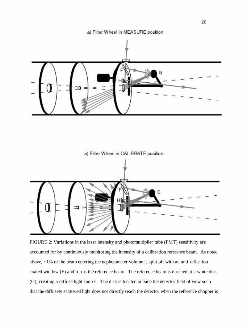
FIGURE 2: Variations in the laser intensity and photomultiplier tube (PMT) sensitivity are

accounted for by continuously monitoring the intensity of a calibration reference beam. As noted

above, ~1% of the beam entering the nephelometer volume is split off with an anti-reflection

coated window (F) and forms the reference beam. The reference beam is directed at a white disk

(G), creating a diffuse light source. The disk is located outside the detector field of view such

that the diffusely scattered light does not directly reach the detector when the reference chopper is

27

in the open (measure) position. (a). The diffuse light strikes baffles and walls coated with black

optical paint, and is largely absorbed. When the reference chopper is in the "calibrate" position,

some of the diffuse light strikes a neutral-density coated glass surface, transmitting some of the

light to the detector (b). Variations in laser intensity are manifested as changes in the "calibrate"

photon counts, C cal, which are used to calculate the system signal as described in the text.

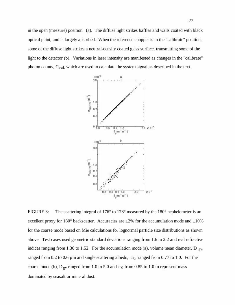
FIGURE 3: The scattering integral of 176° to 178° measured by the 180° nephelometer is an

excellent proxy for 180° backscatter. Accuracies are ±2% for the accumulation mode and ±10%

for the coarse mode based on Mie calculations for lognormal particle size distributions as shown

above. Test cases used geometric standard deviations ranging from 1.6 to 2.2 and real refractive

indices ranging from 1.36 to 1.52. For the accumulation mode (a), volume mean diameter, D gv,

ranged from 0.2 to 0.6 µm and single scattering albedo, ω0, ranged from 0.77 to 1.0. For the

coarse mode (b), D gv ranged from 1.0 to 5.0 and ω0 from 0.85 to 1.0 to represent mass

dominated by seasalt or mineral dust.

28

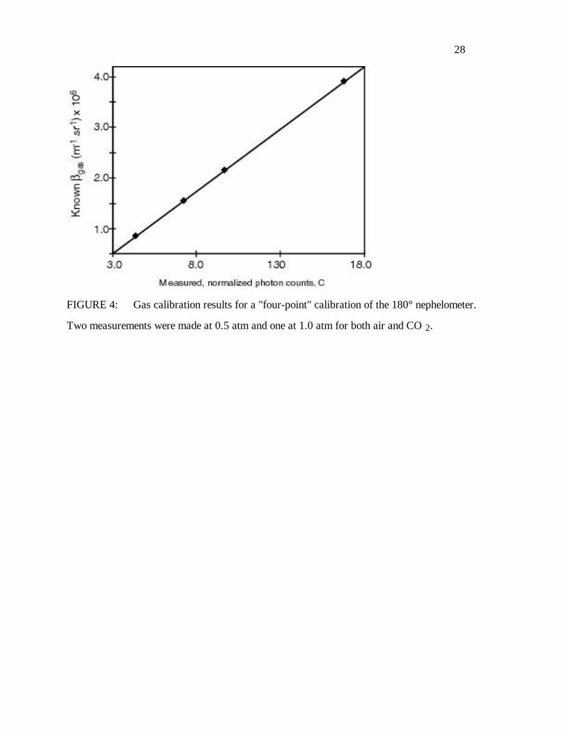
FIGURE 4: Gas calibration results for a "four-point" calibration of the 180° nephelometer.

Two measurements were made at 0.5 atm and one at 1.0 atm for both air and CO 2.

29

FIGURE 5: Optical properties of continental aerosol measured on March 5, 1998 GMT (day

64) at Cheeka Peak Observatory, Washington.

30

FIGURE 6: Optical properties of marine aerosol measured on March 16, 1998 GMT (day 75)

at Cheeka Peak Observatory, Washington.