measurement of the mqe parameter using multiple … · a parameter using multiple quasi-elastic...
TRANSCRIPT

MEASUREMENT OF THEMQEA PARAMETER USING MULTIPLE
QUASI-ELASTIC DOMINATED SUB-SAMPLES IN THE MINOS NEAR
DETECTOR
Nathan S. Mayer
Submitted to the faculty of the University Graduate School
in partial fulfillment of the requirements
for the degree
Doctor of Philosophy
in the Department of Physics,
Indiana University
December 2011
ii
Accepted by the Graduate Faculty, Indiana University, in partial fulfillment of the
requirements for the degree of Doctor of Philosophy.
Doctoral Committee
Mark Messier, Ph.D.
Rex Tayloe
Jon Urheim
Mike Snow
Date of Oral Examination
December 5, 2011

iii
Copyright c©2011
Nathan Mayer

iv
For Gloria, who taught me to reach for the stars, but made surethat my feet stayed
grounded here on earth. I miss you, Grandma.

Acknowledgements
I have been training to be a physicist for the last thirteen years of my life. I’ve
spent so much of my life working to become a scientist that being a scientist is
as important to my personal identity as breathing is to sustaining life. The people
who’s influence helped me to become the person that I am, also shaped me into
the physicist that I’ve become. The same is true of the peoplewho trained me to
be the physicist, they have helped to make me the person that I’ve become.
First I need to thank two people without whom this dissertation would not
have been possible. Mark Dorman, who developed the core codethat was used to
fit for the quasi-elastic axial mass, if it weren’t for Mark I would still be writing
the infrastructure code. Mark also provided a great deal of assistance, helping me
understand the Llewellyn Smith model. During my time at Duluth Aaron Mislivec
developed an early version of the algorithm that’s used to find candidate proton
tracks, with out his early work this analysis would look verydifferent.
I owe more thanks than I could possible express to my advisor Mark Messier.
Mark encouraged me to take on an analysis, that was outside ofhis comfort zone.
Than proceeded to find out everything he could about quasi-elastic neutrino inter-
actions, so that I could write the best dissertation I could.His constant encourage-
ment, and feedback have made me a better scientist and betterperson. If I become
half the scientist he already is than I will have become an exceptional scientist.
The first time I applied to graduate school I did so unsuccessfully, with univer-
sal denials from every doctoral program the I applied to. I applied to UMD as a
hail mary, fortunately the physics department allowed to meregister as a graduate
v
vi
student that year. Rik was my advisor at UMD, he provided my first real exposure
to being a scientist. His unremitting thoroughness for the details of an analysis,
though annoying at times (”OK, you know what you should try next...”) is exactly
what a person like me needed when I was first learning how to be ascientist.
Thanks also go to my defense committee Rex, Mike, and Jon, do to unforeseen
circumstances I needed to scramble very near my defense deadline to replace a few
of the original committee members. I’ve worked with all of you in some context
over the last few years. You’ve all taught me quite a lot and for that you have my
gratitude.
My eternal appreciation goes to the IU high energy neutrino research group
for providing me with the guidance and companionship over the last few years I
could not have completed my degree with it. Further thanks goto the group along
with the US DOE for providing the funding that allowed me to attend graduate
school.
I would never have been able to go from a twelve page analysis note to a
two hundred and three page dissertation draft in two and a half months without
the support of my girlfriend Jen, her unwavering belief thatI could finish the
dissertation in time is what kept me going. That same draft would have been
much less readable without the weekend that she spent editing it. Thank you.
I’ve never heard any one describe getting through graduate school as easy,
the only thing that makes the experience of graduate school bearable is sharing
the experience with others who’re going through the same thing. For me those
people were the graduate students and young post-docs of Young MINOS: Dan,
Mark, Zeynep, Alex H., Alex R., Mhair, Ruth, Chris, Jess, andmany others who’s
names I’m forgetting right now. Whether it’s going out for a pint in the evening
during collaboration meetings, sharing programming tips,or commiserating about
the unreasonable Professor (or Convener) who really isn’t unreasonable, I never
would have be able to make it through the last couple of years without them.
Most importantly I need to thank my mom and dad (Al and Lorri) and my
grandpa and grandma (Marvin and Gloria), they each played more than a small
vii
part in the person that I have grown into, and the scientist that I hope to one day
become. My dad was always willing to talk to me about science,whether it was
the mysteries of human consciousness or the weirdness Quantum Mechanics, our
conversations inspired a deep curiosity that brought me to science. My moth-
ers deep love of nature and all things green, instilled in me asimilar love that
drives me to look for the beauty that exists in the natural world and is inherent
to it’s fundamental laws. In science “failures” greatly outnumber successes, my
grandfather’s stoicism and quite compassion infused me with the patience to ac-
cept and move past these numerous failures while continuingto work towards the
infrequent successes. Finally my grandmother (for whom this dissertation is ded-
icated) always treated me like the adult she new I could be, and when necessary
treated me like the child I was (or was acting like). This dissertation is dedicated
to her because she wasn’t able to see me complete it.
viii
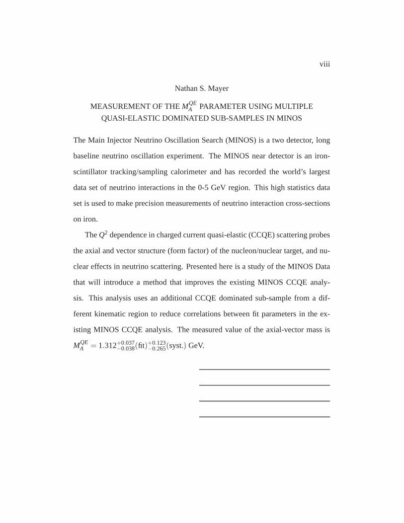
Nathan S. Mayer
MEASUREMENT OF THEMQEA PARAMETER USING MULTIPLE
QUASI-ELASTIC DOMINATED SUB-SAMPLES IN MINOS
The Main Injector Neutrino Oscillation Search (MINOS) is a two detector, long
baseline neutrino oscillation experiment. The MINOS near detector is an iron-
scintillator tracking/sampling calorimeter and has recorded the world’s largest
data set of neutrino interactions in the 0-5 GeV region. Thishigh statistics data
set is used to make precision measurements of neutrino interaction cross-sections
on iron.
TheQ2 dependence in charged current quasi-elastic (CCQE) scattering probes
the axial and vector structure (form factor) of the nucleon/nuclear target, and nu-
clear effects in neutrino scattering. Presented here is a study of the MINOS Data
that will introduce a method that improves the existing MINOS CCQE analy-
sis. This analysis uses an additional CCQE dominated sub-sample from a dif-
ferent kinematic region to reduce correlations between fit parameters in the ex-
isting MINOS CCQE analysis. The measured value of the axial-vector mass is
MQEA = 1.312+0.037
−0.038(fit)+0.123−0.265(syst.) GeV.
Contents
1 Introduction 1
1.1 Introduction . . . . . . . . . . . . . . . . . . . . . . . . . . . . 1
1.2 Neutrino Oscillation Theory . . . . . . . . . . . . . . . . . . . 4
1.3 Neutrino Oscillations in MINOS . . . . . . . . . . . . . . . . . 5
1.4 Motivation for Neutrino Quasi-Elastic Measurements . .. . . . 8
2 Theory of the Weak Interaction 11
2.1 Weak Interaction Phenomenology . . . . . . . . . . . . . . . . 11
2.1.1 Fermi’s Point-like Four-Fermion Theory ofβ-Decay . . 11
2.1.2 The Axial Vector Structure of the Weak Interaction . . .13
2.1.3 Helicity and Chirality . . . . . . . . . . . . . . . . . . . 16
2.1.4 Electroweak Gauge Theory . . . . . . . . . . . . . . . . 18
2.2 Neutrino-Nucleus Scattering . . . . . . . . . . . . . . . . . . . 23
2.2.1 Neutrino Scattering Off of Nucleons . . . . . . . . . . . 23
2.2.2 Neutrino-Nucleon Scattering Kinematics . . . . . . . . . 24
2.2.3 Nucleon Form Factors and the QE Cross Section . . . . 27
2.2.4 Nuclear Effects . . . . . . . . . . . . . . . . . . . . . . 32
3 Survey of Current Results 39
3.1 Generalized Method for MeasuringMQEA . . . . . . . . . . . . . 39
3.2 Summary of World Average Values . . . . . . . . . . . . . . . . 40
3.3 Survey ofMQEA Measurements . . . . . . . . . . . . . . . . . . 44
3.3.1 Argonne 12-Foot Bubble Chamber . . . . . . . . . . . . 44
ix

CONTENTS x
3.3.2 Results From the NOMAD Experiment . . . . . . . . . 48
3.3.3 Results From the MiniBooNE Experiment . . . . . . . . 50
3.4 Resolving the MiniBooNE-NOMAD Discrepancy . . . . . . . . 55
4 MINOS Experiment 58
4.1 The NuMI Beamline . . . . . . . . . . . . . . . . . . . . . . . 58
4.2 The MINOS Detectors . . . . . . . . . . . . . . . . . . . . . . 62
4.2.1 Common Detector Features . . . . . . . . . . . . . . . . 63
4.2.2 The Calibration Detector . . . . . . . . . . . . . . . . . 65
4.2.3 The Far Detector . . . . . . . . . . . . . . . . . . . . . 66
4.2.4 The Near Detector . . . . . . . . . . . . . . . . . . . . 68
5 MINOS Data and Monte Carlo 72
5.1 MINOS Data . . . . . . . . . . . . . . . . . . . . . . . . . . . 72
5.1.1 Reconstruction . . . . . . . . . . . . . . . . . . . . . . 72
5.1.2 Calibration . . . . . . . . . . . . . . . . . . . . . . . . 77
5.2 MINOS MC . . . . . . . . . . . . . . . . . . . . . . . . . . . . 83
5.2.1 Beam Re-Weighting . . . . . . . . . . . . . . . . . . . 85
6 Event Selection 91
6.1 νµ-CC Event Selection . . . . . . . . . . . . . . . . . . . . . . 91
6.1.1 Beam Quality Criteria . . . . . . . . . . . . . . . . . . . 92
6.1.2 Near Detector Event Quality Criteria: . . . . . . . . . . 93
6.1.3 Charged Current Preselection . . . . . . . . . . . . . . . 94
6.1.4 νµ-CC Multivariate Identification Parameter . . . . . . . 95
6.2 Partial Proton Track Reconstruction . . . . . . . . . . . . . . . 99
6.2.1 Reconstruction Algorithm . . . . . . . . . . . . . . . . 100
6.3 The Interaction Sub-Sample Selections . . . . . . . . . . . . . .104
6.3.1 Low Hadronic Energy Quasi-Elastic Like Selection . . .105
6.3.2 Two Track Quasi-Elastic Like Selection . . . . . . . . . 107
6.3.3 Two Track Background Like Selection . . . . . . . . . . 107
CONTENTS xi
6.3.4 Selection Purity and Efficiency . . . . . . . . . . . . . . 109
6.4 Comparisons of Data to Monte Carlo . . . . . . . . . . . . . . . 110
6.4.1 Nuclear Correlations in MINOS . . . . . . . . . . . . . 118
7 Extracting the Axial-Vector Mass 120
7.1 Fitting Procedure and Fit Parameters . . . . . . . . . . . . . . . 120
7.2 Mock Data Analysis . . . . . . . . . . . . . . . . . . . . . . . . 126
7.2.1 Mock Data Construction . . . . . . . . . . . . . . . . . 126
7.2.2 Mock Data Fit Results . . . . . . . . . . . . . . . . . . 127
7.2.3 Conclusion . . . . . . . . . . . . . . . . . . . . . . . . 128
7.3 Initial Fit to Data . . . . . . . . . . . . . . . . . . . . . . . . . 128
7.4 Fit Using The Resonance Suppression Function . . . . . . . . .133
7.5 New Fit Procedure . . . . . . . . . . . . . . . . . . . . . . . . . 137
7.5.1 Fit Steps . . . . . . . . . . . . . . . . . . . . . . . . . . 137
7.5.2 Hadronic Shower Energy Offset . . . . . . . . . . . . . 139
7.5.3 Fit Results . . . . . . . . . . . . . . . . . . . . . . . . . 140
7.5.4 Systematic Error Contribution . . . . . . . . . . . . . . 141
7.5.5 Best Fit Confidence Regions . . . . . . . . . . . . . . . 154
7.6 Conclusion . . . . . . . . . . . . . . . . . . . . . . . . . . . . 159
8 Interpreting the Results 160
8.1 Nuclear Effects . . . . . . . . . . . . . . . . . . . . . . . . . . 160
8.2 Analysis Improvements . . . . . . . . . . . . . . . . . . . . . . 162
8.2.1 Selection Criteria Systematic . . . . . . . . . . . . . . . 162
8.2.2 Background Modeling . . . . . . . . . . . . . . . . . . 164

List of Figures
1.1 Survival probability of muon neutrinos as a function of energy
given the MINOS baseline and best fit values for the oscillation
parameters. The first minimum from the right is the dip that MI-
NOS is most sensitive to. . . . . . . . . . . . . . . . . . . . . 4
1.2 From [10]. Top: The MINOS energy spectra of fully recon-
structed events in the Far Detector classified as charged current
interactions. The dashed histogram represents the spectrum pre-
dicted from measurements in the Near Detector assuming no os-
cillations, while the solid histogram reflects the best fit ofthe
oscillation hypothesis. The shaded area shows the predicted neu-
tral current background. Bottom: The points with error barsare
the background-subtracted ratios of data to the no-oscillation hy-
pothesis. Lines show the best fits for: oscillations, decay [11],
and decoherence [12]. . . . . . . . . . . . . . . . . . . . . . . 6
1.3 From [10]. Likelihood contours of 68% and 90% C.L. around
the best fit values for the mass splitting and mixing angle. Also
shown are contours from previous measurements [13, 14]. . . 7
1.4 The expected 1 and 2σ measurements of sin2(2θ23) for 6 years
of NOvA running (3 yrs in neutrino mode +3 yrs in anti-neutrino
mode) using numu quasi elastic events in NOvA. The input∆m2
is taken to coincide with recent MINOS measurements and the
three choices of mixing angle are made consistent with the data
from Super-Kamiokande (>0.92 at 90% confidence limit). . . 9
xii

LIST OF FIGURES xiii
2.1 Feynman diagram of the muon decay process (µ− → νµ+ νee−) 21
2.2 CCνµ−N scattering kinematics. Inside the red boxes are the
variables that are measured in the MINOS detectors (in the lab
frame). The diagram also labels the four-momentum of the par-
ticles in the center of mass frame. The Bjorken scaling variable,
x, denotes the fraction of the nucleon momentum carried by the
struck quark. . . . . . . . . . . . . . . . . . . . . . . . . . . . 25
2.3 Feynman diagram of theνµ-CC QE interaction, showing both the
νµ, W+, µ− and then, W+, p vertices. . . . . . . . . . . . . . 27
2.4 Above: quasi-elastic differential cross section off ofa free nu-
cleon with respect toQ2. Each distribution corresponds to a
different value of the axial-vector mass parameter. Below:The
sameQ2 distribution as above except the red and blue distribu-
tions are normalized to the area of the blackQ2 distribution. . 33
2.5 The CC-νµ QE differential cross section with respect toQ2 with
several values ofkF compared to the free nucleon case, shows
the low Q2 suppression characteristic of Pauli-blocking. Taken
from a talk given by M. Sakuda at the 2005 NuFact conference. 36
2.6 The MiniBooNEνµ CCQE cross section as a function of the
incident neutrino energy. The points are the MiniBooNE data,
the red line is theνµ CCQE cross section with anMQEA value of
1.02 GeV and including the effect of the most important typesof
SRC interactions. The black dashed line is the sameνµ CCQE
cross section without the SRT interactions. There is remarkable
agreement between the MiniBooNE data and theQE+ np−nh
model. This agreement indicates that the 20-30% discrepancy in
the recent high statistics interaction experiments could,in part,
be due to these SRC type interactions. . . . . . . . . . . . . . 37
LIST OF FIGURES xiv
3.1 Q2 distribution from [42]. The data corresponds to the shown
histogram, the solid curve corresponds to the dipole axial-vector
form factor utilizing the best fit from the flux independent analy-
sis from Table 3.2. The dotted curve corresponds to an alternate
form of the axial-vector form factor withMQEA = 1.11 GeV. . . 47
3.2 From [52]. Comparison the NOMAD〈σqel〉νµ measurements as
a function of the neutrino energy in the 1-track and 2-track sub-
samples. . . . . . . . . . . . . . . . . . . . . . . . . . . . . . 49
3.3 From [31]. ReconstructedQ2 for νµ CCQE events including sys-
tematic errors. The simulation, before (dashed) and after (solid)
the fit, is normalized to data. The dotted (dot-dash) curve shows
backgrounds that are not CCQE (not “CCQE-like”). The inset
shows the 1σ CL contour for the best-fit parameters (star), along
with the starting values (circle), and fit results after varying the
background shape (triangle). . . . . . . . . . . . . . . . . . . 52
3.4 From [34]. Distribution of events inQ2 QE for the (a) 2 and
(b) 3 subevent samples before the application of the CC1 back-
ground correction. Data and MC samples are shown along with
the individual MC contributions from CCQE, CC1π, and other
channels. In (b), the dashed line shows the CC1π reweighting
function (with the y-axis scale on the right) as determined from
the background t procedure. . . . . . . . . . . . . . . . . . . . 53
LIST OF FIGURES xv
3.5 From [34]. Flux-unfolded MiniBooNEνµ CCQE cross section
per neutron as a function of neutrino energy. In (a), shape errors
are shown as shaded boxes along with the total errors as bars.In
(b), a larger energy range is shown along with results from the
LSND [61] and NOMAD [52] experiments. Also shown are pre-
dictions from the NUANCE simulation for an RFG model with
two different parameter variations and for scattering fromfree
nucleons with the world-average MA value. Numerical values
are provided in Table X in the appendix (of [34]). . . . . . . . 54
3.6 From [62]. Left: The QE differential cross section (dσ/dQ2) as
a function ofQ2 for νµ, νµ energies of 1.0 GeV (maximum ac-
cessibleQ2max= 1.3 (GeV/c)2). Here, the orange dotted line is
the prediction of the ”Independent Nucleon (MA=1.014)” model.
The blue dashed line is the prediction of the the ”LargerMA
(MA=1.3)” model. The red line is prediction of the ”Transverse
Enhancement” model. Top (a):νµ differential QE cross sec-
tions. Bottom (b): νµ differential QE cross sections. Right:
Same as Left forνµ, νµ energies of 3.0 GeV (maximum acces-
sibleQ2max= 4.9 (GeV/c)2). . . . . . . . . . . . . . . . . . . 56
4.1 From [66]. Geograpical view of the MINOS experimental lay-
out. . . . . . . . . . . . . . . . . . . . . . . . . . . . . . . . 59
4.2 From [66]. The layout of the various FNAL proton accelerators. 60
4.3 From [66]. The NuMI target. . . . . . . . . . . . . . . . . . . 60
4.4 From [66]. Left: Photograph of inner conductors of the NuMI
parabolic focusing horn. Right: Photograph of the first focusing
horn. . . . . . . . . . . . . . . . . . . . . . . . . . . . . . . . 61
4.5 From [66]. The various components of the NuMI beamline. .. 62
4.6 From [66]. Left: Individual scintillator strip. Right:Strips that
have collected into a detector module. . . . . . . . . . . . . . 64
4.7 From [66]. Schematic of a scintillator plane readout system. . 65

LIST OF FIGURES xvi
4.8 From [66]. Photograph of the MINOS Calibration detector. . . 66
4.9 From [66]. Photograph of the completed Far detector. . . .. . 67
4.10 From [66]. Photograph of the Near detector. . . . . . . . . . .69
4.11 From [65]. Strip configuration of the MINOS ND, divided into
partially instrumented (above) and fully instrument (below)planes,
and also U-view (left) and V-view (right) planes. . . . . . . . . 70
5.1 From [65]. Stopping power for muons. The gray line shows
the Bethe-Bloch calculation of the stopping power for muons
in polystyrene scintillator. The solid circles and open triangles
show the response of stopping muons in the far detector data and
GEANT3 Monte Carlo simulations respectively. Both data and
Monte Carlo points have been normalized to the Bethe-Bloch
calculation to give the expected stopping power at the minimum
ionizing point. . . . . . . . . . . . . . . . . . . . . . . . . . . 75
5.2 From [71]. Variations in the median signal per plane deposited
by through-going cosmic-ray muons observed during the data-
taking period covered by this paper. The time dependence is
largely due to variations in the environmental conditions in the
Near and Far Detector halls and aging of the scintillator. The
zero point on the ordinate is arbitrary. . . . . . . . . . . . . . 78
5.3 From [65]. Nonlinearity calibration of near and far detector in-
strumentation. The intrinsic nonlinearity of PMT response(cir-
cles) and its residual after calibration (error bars only) are shown
for the near (a) and far (b) detectors. The error bars depict the
rms spread of channels in each detector. For scale, a minimum
ionizing particle normal to the plane will generate roughly500-
600 ADCs of charge each detector. A single photoelectron is
roughly 75 ADCs (Far) or 100 ADCs (Near). . . . . . . . . . 79
LIST OF FIGURES xvii
5.4 From [65]. Mean value of the strip-end responses normalized to
the detector average. The mean response of the strip ends varies
by approximately 29%. The solid and dashed lines are the cal-
culated responses of two separate data sets from June 2005. The
statistical variation in the individual calibration constants from
these two data sets is on the order of 2.1%. . . . . . . . . . . . 80
5.5 From [65]. Comparison of cosmic ray muon data (points) with
module mapper fitting results (solid curve) for a typical strip in
the near detector. . . . . . . . . . . . . . . . . . . . . . . . . 81
5.6 From [65]. MINOS calorimetric response to pions and electrons
at three momenta. The calorimeter-signal scale is in arbitrary
units. The data (open symbols), obtained from the calibration
detector exposure to CERN test beams, are compared to distri-
butions from Monte Carlo simulations. . . . . . . . . . . . . . 82
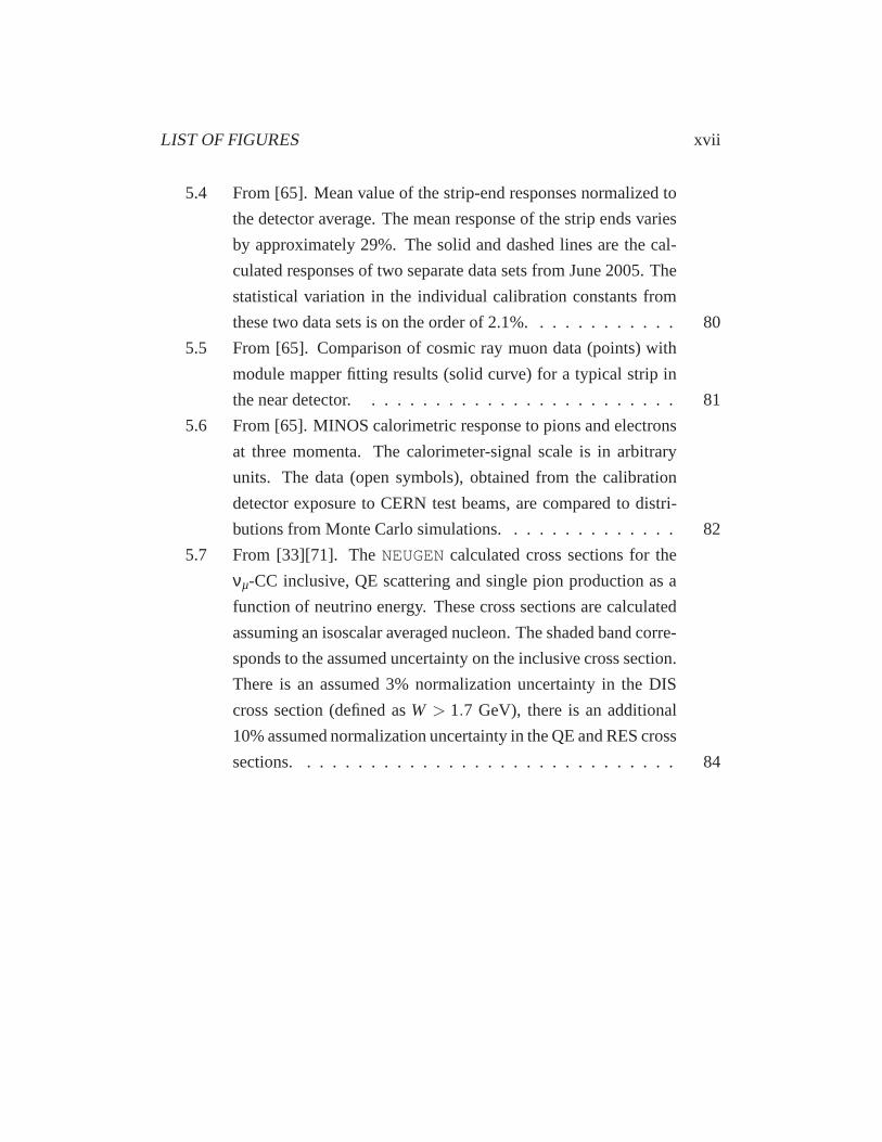
5.7 From [33][71]. TheNEUGEN calculated cross sections for the
νµ-CC inclusive, QE scattering and single pion production as a
function of neutrino energy. These cross sections are calculated
assuming an isoscalar averaged nucleon. The shaded band corre-
sponds to the assumed uncertainty on the inclusive cross section.
There is an assumed 3% normalization uncertainty in the DIS
cross section (defined asW > 1.7 GeV), there is an additional
10% assumed normalization uncertainty in the QE and RES cross
sections. . . . . . . . . . . . . . . . . . . . . . . . . . . . . . 84
LIST OF FIGURES xviii
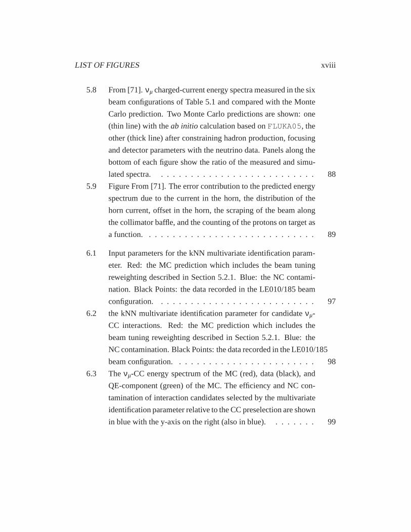
5.8 From [71].νµ charged-current energy spectra measured in the six
beam configurations of Table 5.1 and compared with the Monte
Carlo prediction. Two Monte Carlo predictions are shown: one
(thin line) with theab initio calculation based onFLUKA05, the
other (thick line) after constraining hadron production, focusing
and detector parameters with the neutrino data. Panels along the
bottom of each figure show the ratio of the measured and simu-
lated spectra. . . . . . . . . . . . . . . . . . . . . . . . . . . 88
5.9 Figure From [71]. The error contribution to the predicted energy
spectrum due to the current in the horn, the distribution of the
horn current, offset in the horn, the scraping of the beam along
the collimator baffle, and the counting of the protons on target as
a function. . . . . . . . . . . . . . . . . . . . . . . . . . . . . 89
6.1 Input parameters for the kNN multivariate identification param-
eter. Red: the MC prediction which includes the beam tuning
reweighting described in Section 5.2.1. Blue: the NC contami-
nation. Black Points: the data recorded in the LE010/185 beam
configuration. . . . . . . . . . . . . . . . . . . . . . . . . . . 97
6.2 the kNN multivariate identification parameter for candidateνµ-
CC interactions. Red: the MC prediction which includes the
beam tuning reweighting described in Section 5.2.1. Blue: the
NC contamination. Black Points: the data recorded in the LE010/185
beam configuration. . . . . . . . . . . . . . . . . . . . . . . . 98
6.3 Theνµ-CC energy spectrum of the MC (red), data (black), and
QE-component (green) of the MC. The efficiency and NC con-
tamination of interaction candidates selected by the multivariate
identification parameter relative to the CC preselection are shown
in blue with the y-axis on the right (also in blue). . . . . . . . 99

LIST OF FIGURES xix
6.4 True kinetic energy of the leading proton in true QE events. The
majority, 95%, of the recoil have energy less than 1 GeV, nearly
99% have energy less than 2 GeV. . . . . . . . . . . . . . . . 101
6.5 Event display of a characteristic true QE event in MINOS.On the
top is the full event before any of the hit filters are applied.The
plot on the bottom illustrates the grouping algorithm at work. In
this case the line is drawn between the event vertex and the red
hit that is in the candidate proton track furthest down stream from
the event vertex. The black boxes represent the regions included
in the grouping algorithm. Any hits whose hit centers are within
one of the black boxes will be counted as part of the candidate
proton track. . . . . . . . . . . . . . . . . . . . . . . . . . . . 102
6.6 Left: The opening angle between the MC true proton momen-
tum and the reconstructed proton trajectory for all two track QE
selected events. Right: The opening angle between the MC true
proton momentum and the reconstructed proton trajectory for all
MC true CCQE events with a candidate proton track. The “shoul-
der” near 60◦ in the plot on the right is due to incomplete removal
of the muon track. When there is more than 600 sigcor of pulse
height near the event vertex, and the true proton is below detec-
tion threshold, it is possible for this algorithm to get confused
and interpret the remaining muon hits as coming from a proton.
This effect is illustrated in Figure 6.5. In the bottom panelof
Figure 6.5 there are clearly two hits that were left over fromthe
muon track. It is these hits that could potentially confuse this
algorithm and create this shoulder. . . . . . . . . . . . . . . . 103
6.7 The reconstructed hadronic shower energy of the neutrino event.
The histograms show the dominant NEUGEN interaction types.
The event is flagged as QE like if the the reconstructed hadronic
shower energy is less than 0.25 GeV . . . . . . . . . . . . . . 106

LIST OF FIGURES xx
6.8 Left: The fraction of true QE interactions in the given selection.
Right: The efficiency of selecting true QE interactions relative to
the number of true QE interactions in theνµ-CC selection. The
one track QE selection is in black, the two track QE is blue, and
the two track background selection is red. . . . . . . . . . . . 109
6.9 Left: The fraction of true resonance interactions in thegiven se-
lection. Right: The efficiency of selecting true resonance inter-
actions relative to the number of true resonance interactions in
theνµ-CC selection. The one track QE selection is in black, the
two track QE is blue, and the two track background selection is
red. . . . . . . . . . . . . . . . . . . . . . . . . . . . . . . . 110
6.10 Number hits in the candidate proton track. Top: Pre-selected
(νµ CC) events. Middle: Two track background selection. Bot-
tom: Selected two track QE events. Left: Distributions withMC
normalized to total data POT. Individual topological components
of of the MC are shown as stacked histograms. Right: Ratio of
data to MC. . . . . . . . . . . . . . . . . . . . . . . . . . . . 112
6.11 Summed pulse height of the scintillator strips in the candidate
proton track. Top: Pre-selected (νµ CC) events. Middle: Two
track background selection.Bottom: Selected two track QE events.
Left: Distributions with MC normalized to total data POT. Indi-
vidual topological components of of the MC are shown as stacked
histograms. Right: Ratio of data to MC. . . . . . . . . . . . . 113
6.12 Total path length of the candidate proton track. Top: Pre-selected
(νµ CC) events. Middle: Two track background selection. Bot-
tom: Selected two track QE events. Left: Distributions withMC
normalized to total data POT. Individual topological components
of of the MC are shown as stacked histograms. Right: Ratio of
data to MC. . . . . . . . . . . . . . . . . . . . . . . . . . . . 114

LIST OF FIGURES xxi
6.13 Distance between maximum pulse height hit and furthestdown-
stream hit. Top: Pre-selected (νµ CC) events. Middle: Two
track background selection. Bottom: Selected two track QE
events. Left: Distributions with MC normalized to total data
POT. Individual topological components of of the MC are shown
as stacked histograms. Right: Ratio of data to MC. . . . . . . 115
6.14 Number of unused hits in the vertex hadronic shower. Top: Pre-
selected (νµ CC) events. Middle: Two track background selec-
tion. Bottom: Selected two track QE events. Left: Distribu-
tions with MC normalized to total data POT. Individual topolog-
ical components of of the MC are shown as stacked histograms.
Right: Ratio of data to MC. . . . . . . . . . . . . . . . . . . . 116
6.15 Opening angle between the candidate proton track and the pro-
ton trajectory predicted from muon kinematics (∆θp). Top: Pre-
selected (νµ CC) events. Middle: Two track background selec-
tion. Bottom: Selected two track QE events. Left: Distribu-
tions with MC normalized to total data POT. Individual topolog-
ical components of of the MC are shown as stacked histograms.
Right: Ratio of data to MC. . . . . . . . . . . . . . . . . . . . 117

LIST OF FIGURES xxii
6.16 Summed pulse height in sigcor of all of the hits that are not used
in either the muon track or the candidate proton track. Top:∆θp
sideband selections (QE-like except∆θp > 30). Bottom: Se-
lected two track QE events. Left: Distributions with MC nor-
malized to total data POT. Individual topological components of
of the MC are shown as stacked histograms. Right: Ratio of
data to MC. The MC deficit in the 0-2000 sigcor region of the
top plots when considered along side the MC deficit in the 60-90
degree region of Figure 6.15 is further evidence of a secondary
nucleon from an SRC type interaction. The extra energy that we
are seeing is substantial enough that additional quanta seems like
a more likely explanation than a mis-modeling of detector effects 119
7.1 Comparison of the nominal MC to reweighted MC with±30%
changes to the value ofMQEA . Only stopping muon events are
included in this figure. . . . . . . . . . . . . . . . . . . . . . 122
7.2 Comparison of the nominal MC to scaled MC with±2% scalings
of the muon energy. Only stopping muon events are included in
this figure. . . . . . . . . . . . . . . . . . . . . . . . . . . . . 122
7.3 Comparison of the nominal MC to reweighted MC with±15%
changes to the value ofMRESA . Only stopping muon events are
included in this figure. . . . . . . . . . . . . . . . . . . . . . 123
7.4 Comparison of the nominal MC to MC with a +30% scale of the
values of the Fermi momentum for protons and neutrons. Only
stopping muon events are included in this figure. . . . . . . . . 124
7.5 Comparison of the nominal MC to MC with a±30% scale on the
values of the Fermi momentum for protons and neutrons applied
to the background like two track selection. Only stopping muon
events are included in this figure. . . . . . . . . . . . . . . . . 125
LIST OF FIGURES xxiii
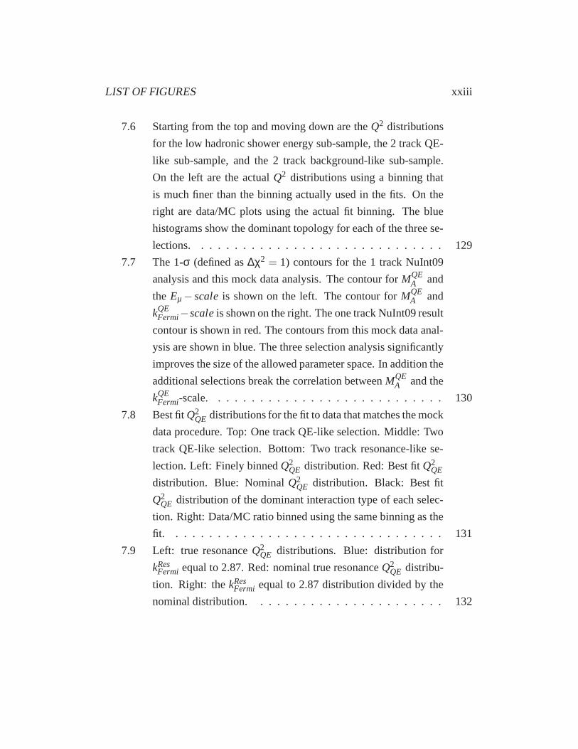
7.6 Starting from the top and moving down are theQ2 distributions
for the low hadronic shower energy sub-sample, the 2 track QE-
like sub-sample, and the 2 track background-like sub-sample.
On the left are the actualQ2 distributions using a binning that
is much finer than the binning actually used in the fits. On the
right are data/MC plots using the actual fit binning. The blue
histograms show the dominant topology for each of the three se-
lections. . . . . . . . . . . . . . . . . . . . . . . . . . . . . . 129
7.7 The 1-σ (defined as∆χ2 = 1) contours for the 1 track NuInt09
analysis and this mock data analysis. The contour forMQEA and
the Eµ− scaleis shown on the left. The contour forMQEA and
kQEFermi−scaleis shown on the right. The one track NuInt09 result
contour is shown in red. The contours from this mock data anal-
ysis are shown in blue. The three selection analysis significantly
improves the size of the allowed parameter space. In addition the
additional selections break the correlation betweenMQEA and the
kQEFermi-scale. . . . . . . . . . . . . . . . . . . . . . . . . . . . 130
7.8 Best fitQ2QE distributions for the fit to data that matches the mock
data procedure. Top: One track QE-like selection. Middle: Two
track QE-like selection. Bottom: Two track resonance-likese-
lection. Left: Finely binnedQ2QE distribution. Red: Best fitQ2
QE
distribution. Blue: NominalQ2QE distribution. Black: Best fit
Q2QE distribution of the dominant interaction type of each selec-
tion. Right: Data/MC ratio binned using the same binning as the
fit. . . . . . . . . . . . . . . . . . . . . . . . . . . . . . . . . 131
7.9 Left: true resonanceQ2QE distributions. Blue: distribution for
kResFermi equal to 2.87. Red: nominal true resonanceQ2
QE distribu-
tion. Right: thekResFermi equal to 2.87 distribution divided by the
nominal distribution. . . . . . . . . . . . . . . . . . . . . . . 132
LIST OF FIGURES xxiv
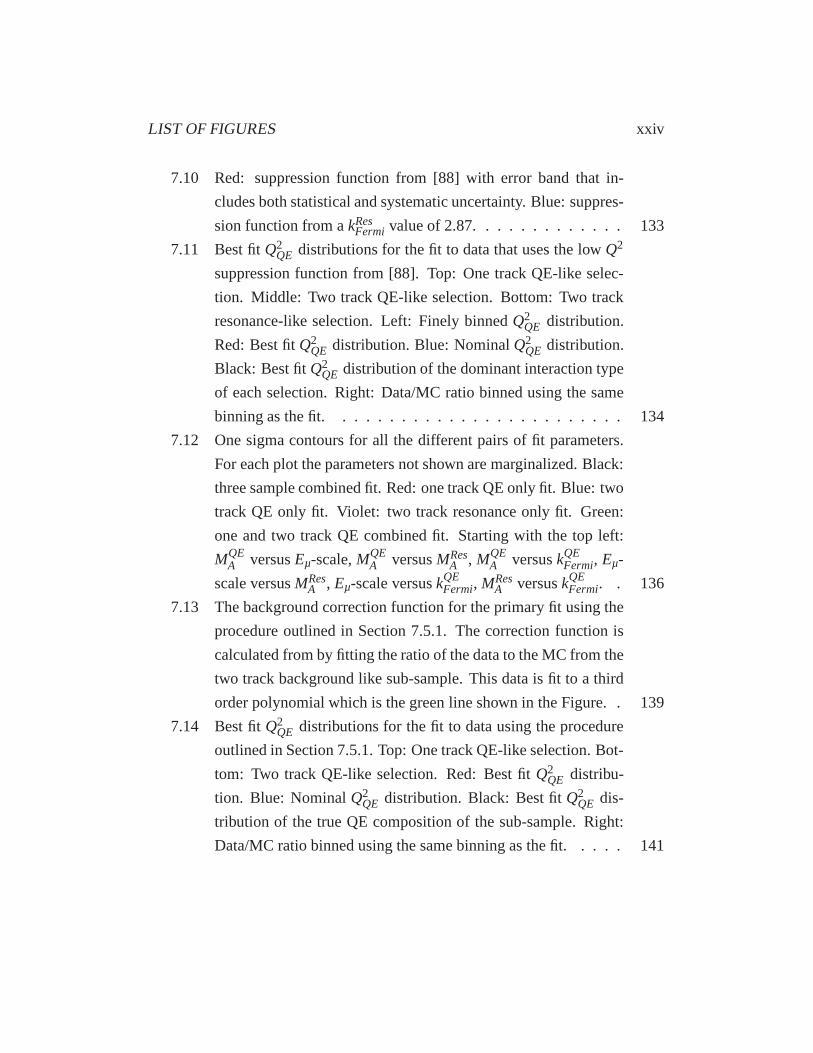
7.10 Red: suppression function from [88] with error band that in-
cludes both statistical and systematic uncertainty. Blue:suppres-
sion function from akResFermi value of 2.87. . . . . . . . . . . . . 133
7.11 Best fitQ2QE distributions for the fit to data that uses the lowQ2
suppression function from [88]. Top: One track QE-like selec-
tion. Middle: Two track QE-like selection. Bottom: Two track
resonance-like selection. Left: Finely binnedQ2QE distribution.
Red: Best fitQ2QE distribution. Blue: NominalQ2
QE distribution.
Black: Best fitQ2QE distribution of the dominant interaction type
of each selection. Right: Data/MC ratio binned using the same
binning as the fit. . . . . . . . . . . . . . . . . . . . . . . . . 134
7.12 One sigma contours for all the different pairs of fit parameters.
For each plot the parameters not shown are marginalized. Black:
three sample combined fit. Red: one track QE only fit. Blue: two
track QE only fit. Violet: two track resonance only fit. Green:
one and two track QE combined fit. Starting with the top left:
MQEA versusEµ-scale,MQE
A versusMResA , MQE
A versuskQEFermi, Eµ-
scale versusMResA , Eµ-scale versuskQE
Fermi, MResA versuskQE
Fermi. . 136
7.13 The background correction function for the primary fit using the
procedure outlined in Section 7.5.1. The correction function is
calculated from by fitting the ratio of the data to the MC from the
two track background like sub-sample. This data is fit to a third
order polynomial which is the green line shown in the Figure.. 139
7.14 Best fitQ2QE distributions for the fit to data using the procedure
outlined in Section 7.5.1. Top: One track QE-like selection. Bot-
tom: Two track QE-like selection. Red: Best fitQ2QE distribu-
tion. Blue: NominalQ2QE distribution. Black: Best fitQ2
QE dis-
tribution of the true QE composition of the sub-sample. Right:
Data/MC ratio binned using the same binning as the fit. . . . . 141

LIST OF FIGURES xxv
7.15 Best fit values (along with theHESSE) errors for different defi-
nitions of the low hadronic energy sub-sample. . . . . . . . . 142
7.16 Best fit values (along with theHESSE errors) for different def-
initions of the∆θp dividing line between the two track QE-like
and two track background like sub-samples. . . . . . . . . . . 143
7.17 Best fit values (along with theHESSE errors) for different defi-
nitions of the unused shower strip hit dividing line betweenthe
two track QE-like and two track background like sub-samples. 144
7.18 Best fit values (along with theHESSE errors) for different defi-
nitions of the unused shower strip hit dividing line betweenthe
two track background like and the sub-sample of interactioncan-
didates that are not used in this analysis. . . . . . . . . . . . . 145
7.19 Best fit values (along with theHESSE errors) for the horn posi-
tion systematic. . . . . . . . . . . . . . . . . . . . . . . . . . 146
7.20 Best fit values (along with theHESSE errors) for the baffle scrap-
ping systematic. . . . . . . . . . . . . . . . . . . . . . . . . . 146
7.21 Best fit values (along with theHESSE errors) for the horn current
calibration systematic. . . . . . . . . . . . . . . . . . . . . . 147
7.22 Best fit values (along with theHESSE errors) for the horn current
distribution systematic. . . . . . . . . . . . . . . . . . . . . . 147
7.23 Best fit values (along with theHESSE errors) for the targetz
position along with hadron production systematics. . . . . . .148
7.24 Best fit values (along with theHESSE errors) for the DIS model
systematic. . . . . . . . . . . . . . . . . . . . . . . . . . . . 149
7.25 Best fit values (along with theHESSE errors) due to the lowQ2
resonance suppression function. . . . . . . . . . . . . . . . . 149
7.26 Best fit values (along with theHESSE errors) for some of the
intranuclear rescattering uncertainties. . . . . . . . . . . . . .150
7.27 Best fit values (along with theHESSE errors) for some of the
intranuclear rescattering uncertainties. . . . . . . . . . . . . .151
LIST OF FIGURES xxvi
7.28 Left: the ratio of data to MC for the nominal MC along withthe
±1σ shifts to the nucleon knockout and nucleon cross section
intranuclear rescattering systematics applied to the nominal MC.
Right: the ratio of the nominal MC to the±1σ nucleon knockout
and nucleon cross section intranuclear rescattering systematics
applied to the nominal MC. Above: the low hadronic energy QE-
like sub-sample. Below: the two track QE-like sub-sample. .. 153
7.29 χ2 scan of the nucleon cross sectionINTRANUKE systematic pa-
rameter. The±1σ uncertainty due to the nucleon cross section
parameter is defined as the fit parameter shift due to a∆χ2 from
the minimum of 1. . . . . . . . . . . . . . . . . . . . . . . . . 154
7.30 χ2 scan of the nucleon knockoutINTRANUKE systematic pa-
rameter. The±1σ uncertainty due to the nucleon cross section
parameter is defined as the fit parameter shift due to a∆χ2 from
the minimum of 1. . . . . . . . . . . . . . . . . . . . . . . . . 155
7.31 Best fit values (along with theHESSE errors) for some of the
intranuclear rescattering uncertainties. . . . . . . . . . . . . .156
7.32 One sigma contour of theMQEA (a scale factor on the nominal
value ofMQEA equal to 0.99 GeV) parameter versus the hadronic
energy offset systematic parameter. The hadronic energy offset
parameter shows very little correlation with any of the other fit
parameters. Thus a plot of any other fit parameter versus the
hadronic energy offset will look very similar to this one. . .. 157
7.33 One sigma contour of theMQEA parameter versus theMRES
A pa-
rameter. Both of these parameters are scale factors on the nom-
inal values of these parameters. The nominal value forMQEA is
0.99 GeV while the nominal value forMRESA is 1.12 GeV. The use
of the two track QE-like and the two track background like sub-
samples breaks the correlations between the both of the axial-
vector parameters. . . . . . . . . . . . . . . . . . . . . . . . . 157
LIST OF FIGURES xxvii
7.34 One sigma contour of theMQEA (a scale factor on the nominal
value of MQEA equal to 0.99 GeV) parameter versus thekQE
Fermi
parameter. The tension between the low hadronic energy offset
sub-sample and the two track QE-like sub-sample largely breaks
the correlation between these parameters. There is still some
correlation in the lower allowed region of the quasi-elastiaxial-
vector mass parameter. . . . . . . . . . . . . . . . . . . . . . 158
7.35 One sigma contour of theMQEA (a scale factor on the nominal
value ofMQEA equal to 0.99 GeV) versus theEµ-scale systematic
parameter. There is a strong correlation between these parame-
ters due to the muon energy dependence ofQ2QE. . . . . . . . 158
8.1 MeasuredMQEA values as a function of the neutrino target nu-
cleon number. Previous measurements are red, while the mea-
surement presented in here is blue. . . . . . . . . . . . . . . . 161
8.2 Left: Q2 distributions used in this analysis along with an alterna-
tive to the low hadronic energy sub-sample called the ‘one track’
sub-sample. Right: the same distributions as the left but ona
semi-log scale. . . . . . . . . . . . . . . . . . . . . . . . . . 163
List of Tables
2.1 The possible forms of the weak interaction that are allowed in
Dirac’s theory . . . . . . . . . . . . . . . . . . . . . . . . . . . 15
2.2 Lorentz invariant kinematic variables that describe the charged
current neutrino-nucleon scattering. The massM is the mass of
the struck nucleon. . . . . . . . . . . . . . . . . . . . . . . . . 26
3.1 Summary of someMQEA measurements. Table reproduced from
[52]. . . . . . . . . . . . . . . . . . . . . . . . . . . . . . . . . 43
3.2 Best fit results forMQEA using the likelihood functions given in
Equations 3.1 to 3.4 as discussed in [42]. . . . . . . . . . . . . 48
5.1 The target position refers to the distance the target wasdisplaced
upstream of its default position inside the rst focusing horn. The
peak (i.e., most probable) neutrino energyEν is determined after
multiplying the muon-neutrino ux predicted by the beam Monte
Carlo simulation by charged-current cross-section. The r.m.s. refers
to the root mean square of the peak of the neutrino energy distri-
bution. The 0 kA “horn-off” beam is unfocused and has a broad
energy distribution. . . . . . . . . . . . . . . . . . . . . . . . . 86
7.1 Best fit results and for the two fit configurations and reduced χ2
values according to 7.1 for the best fit MC. . . . . . . . . . . . 127
7.2 Best fit values for the fit to data. The errors shown are the MINUIT
returned HESSE errors. . . . . . . . . . . . . . . . . . . . . . 130
xxviii
LIST OF TABLES xxix
7.3 Best fit values for the fit to data using the suppression function
from [88]. The errors shown are the MINUIT returned HESSE
errors. . . . . . . . . . . . . . . . . . . . . . . . . . . . . . . . 135
7.4 Best fit values for the baseline first and second fit iteration using
the procedure outlined in Section 7.5.1. No further iterations were
necessary because there was very little change in the background
correction function. The errors shown are theHESSE errors from
theMINUIT software package. . . . . . . . . . . . . . . . . . 140
7.5 Contribution to the systematic error due to the different categories
defined in this Section on theMQEA fit parameter. . . . . . . . . 154
7.6 Best fit values for the along with contributions to the uncertainty
due to the fit and the systematics considered in Section 7.5.4. . . 156

Chapter 1
Introduction
1.1 Introduction
Particle physicists rely on the The Standard Model for the theoretical framework
to describe the interactions of the fundamental particles and forces of the universe.
The Standard Model is one of the most throughly tested and successful theories
of science. However, in the last thirty years, developmentswithin the study of
neutrinos have revealed a weakness in the Standard Model. This is the apparent
flavor-oscillation within the neutrino sector, exemplifiedby the so-called Atmo-
spheric Neutrino Anomaly, and the Solar Neutrino Problem.
The Standard Model describes twelve fundamental fermionicparticles divided
into two separate families: the leptons and the quarks of thehadronic sector. Neu-
trinos belong to the lepton family of which there are three flavors: the electron,
muon and tau neutrinos (νe, νµ, andντ). The Standard Model describes the neu-
trino as massless, chargeless spin-12 particles that also carry no color charge and
only interact via the weak nuclear force. Wolfgang Pauli originally proposed the
existence of the neutrino to solve the problem of apparent momentum noncon-
servation in nuclearβ-decay [1]. The classical two bodyβ-decay isn → p+ e,
under this interaction if energy and momentum are conservedthe electron should
be emitted with discrete energy. However the observed energy of the electron
1

CHAPTER 1. INTRODUCTION 2
from β-decay was a continuous spectrum. The only way the continuous spectrum
of the electron can be explained without violating momentumconservation was
by postulating the existence of an additional particle, nearly impossible to detect,
that carried away a fraction of the total energy. This brilliant though controversial
idea resolved the conflict between momentum conservation and the observed elec-
tron spectrum. It took 26 years to finally confirm Pauli’s hypothesis, when Reines
and Cowen directly observed a neutrino interaction throughthe inverseβ-decay
mechanism at the Savannah River nuclear reactor [?].
The Solar Neutrino Problem is a discrepancy between the number of neutri-
nos interacting in the Earth (and the experiments of physicists) and the expected
number of neutrinos predicted by models of the rates of nuclear reactions within
the sun. The Sun releases energy through nuclear fusion, primarily through the
proton-proton chain. The proton-proton chain converts four hydrogen nuclei into
one helium nucleus, two neutrinos, two positrons and some excess energy. The
Davis and Bahcall experiment at the Homestake mine was the first to measure the
solar neutrino flux. They measured a deficit compared to theoretical predictions
of the solar model [3][4][5].
The Atmospheric Neutrino Anomaly is a discrepancy in the fluxof muon neu-
trinos relative to the flux of electron neutrinos due to cosmic ray interactions in
the upper atmosphere. Cosmic rays incident on the upper atmosphere interact with
nucleons that lie within the constituent molecules of the atmosphere, producing
a shower of secondary and tertiary particles which include large numbers of pi-
ons. The pions eventually decay to muons which will decay to electrons by the
following processes:
π− → µ+ +νµ (1.1)
µ− → e+ +νe+νµ (1.2)
From the very well measured branching ratios of pions, equations 1.1 and 1.2 im-
ply that the ratio ofνµ(νµ) : νe(νe) arriving should be 2 : 1, however experimental
measurements of this ratio have shown a deficit in the number of νµ [6] [7] [8].

CHAPTER 1. INTRODUCTION 3
The solution to both the Solar Neutrino Problem and the Atmospheric Neu-
trino Anomaly was first suggested by Bruno Pontecorvo. In 1967 [9] Pontecorvo
proposed that neutrinos were oscillating between the neutrino’s creation and the
neutrinos detection. Neutrino oscillation is a mixing of the neutrino flavor that is
analogous to flavor changing weak decays in the quark sector.Pontecorvo sug-
gested that if neutrinos had finite mass and if the weak eigenstates of the neutrino
(the interaction state of the neutrino) were not the same as the mass eigenstates of
the neutrino (the propagation state of the neutrino), then amixing matrix could be
formed in a procedure similar to the Cabbibo-Kobayashi-Maskawa (CKM) matrix
of the quarks. Thus a neutrino created in one flavor eigenstate would became a
superposition of all the flavor eigenstates as the neutrinospropagate in the mass
eigenstates. This enables the detection of a different flavor eigenstate at some later
time. This phenomenon can be used to explain both the Solar Neutrino Problem
and the Atmospheric Neutrino Anomaly, though it requires massive neutrinos and
a theory beyond the Standard Model.
Neutrinos have been studied from cosmic ray production, andfrom fission
decay within nuclear reactors. However there are limitations to this approaches.
These limitations are primarily due to having limited control over the conditions of
the neutrino’s creation. The approach of more recent experiments, greater control
over the production conditions of the neutrino, is to use a beam of neutrinos pro-
duced from particle accelerators specialized in the production of neutrino beams.
This is the source for neutrinos used in the Main Injector Neutrino Oscillation
Search (MINOS) experiment, currently running at the Fermi National Accelerator
Laboratory (FNAL) in Batavia, Illinois.
The physics goal of the MINOS experiment is to make a precise measurement
of the parameters that govern muon disappearance (νµ /→νµ). MINOS has been
very successful at this, publishing the world’s most precise measurement of the
atmospheric mass splitting∆m223 [10]. The MINOS experiment uses the neutrino
beam produced by the Neutrinos at the Main Injector (NuMI) facility. This beam
is greater than 95% pure muon neutrino. MINOS measures the composition and
CHAPTER 1. INTRODUCTION 4
spectrum of the neutrino beam by sampling the beam at two locations using large
iron and scintillator tracking/sampling colorimeters; the Near Detector at FNAL
and the Far Detector at the Soudan Underground Laboratory, 734 km away in
Soudan Minnesota. MINOS maximizes their sensitivity to theneutrino oscillation
parameters by comparing the spectrum at the Near Detector, where the neutrinos
have not traveled far enough to have oscillated, to the spectrum at the Far Detector
where the neutrinos will have oscillated (if the oscillations are true).
1.2 Neutrino Oscillation Theory
(GeV)ν E1 10
) µν → µν
P(
0
0.2
0.4
0.6
0.8
1
Survival Probabilityµν
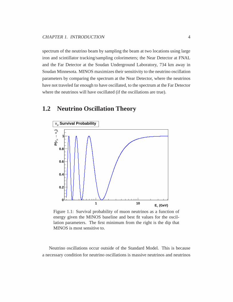
Figure 1.1: Survival probability of muon neutrinos as a function ofenergy given the MINOS baseline and best fit values for the oscil-lation parameters. The first minimum from the right is the dipthatMINOS is most sensitive to.
Neutrino oscillations occur outside of the Standard Model.This is because
a necessary condition for neutrino oscillations is massiveneutrinos and neutrinos
CHAPTER 1. INTRODUCTION 5
have no mass within the Standard Model. Thus neutrinos oscillations are evidence
of “beyond the Standard Model” physics. The probability that a muon neutrino of
a given energy will survive with out oscillating after some distance is given by the
survival probability given by:
P(νβ → νβ(L/E)) = 1−sin22θsin2[1.27∆m2(L/E)]
(1.3)
Equation 1.3 demonstrates that for an experiment that has a fixed baseline (L)
the strength of the oscillation of a neutrino of a given energy E is a function of
only the mixing angleθ and the mass splitting∆m2. The survival probability
for νµ as function of energy as given by equation 1.3 is shown in Figure 1.1.
This plot assumes the MINOS baseline of 734km, sin22θ = 1 and∆m2 = 2.32×10⁻³ GeV2.
1.3 Neutrino Oscillations in MINOS
MINOS looks for an energy dependent disappearance of muon neutrinos at the
Far Detector as compared to the no oscillations expectation. MINOS uses the data
taken at the Near Detector (ND) to validate the Monte Carlo (MC) simulation of
the neutrino interactions. MINOS then extrapolates the neutrino energy spectrum
at the ND, as predicted by the simulation, to the Far Detector. This prediction
assumes that the muon neutrinos are not oscillating into other neutrino flavors.
Deviations between the extrapolated Far Detector spectrum(from the ND) and
the data taken at the Far Detector are then fit to extract the neutrino oscillation
parameters;∆m2 and the mixing angleθ.
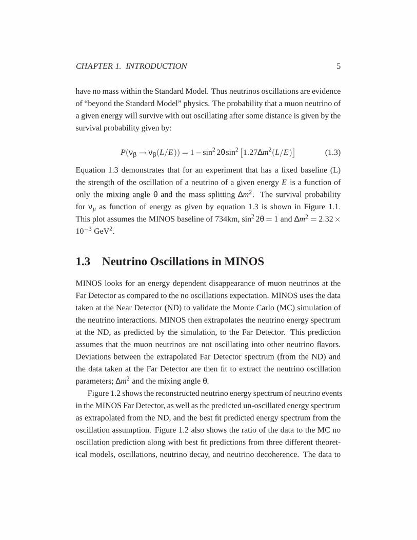
Figure 1.2 shows the reconstructed neutrino energy spectrum of neutrino events
in the MINOS Far Detector, as well as the predicted un-oscillated energy spectrum
as extrapolated from the ND, and the best fit predicted energyspectrum from the
oscillation assumption. Figure 1.2 also shows the ratio of the data to the MC no
oscillation prediction along with best fit predictions fromthree different theoret-
ical models, oscillations, neutrino decay, and neutrino decoherence. The data to
CHAPTER 1. INTRODUCTION 6
Eve
nts
/ GeV
0
100
200
300
MINOS Far Detector
Fully reconstructed events
Data
No oscillations
Best oscillation fit
Neutral current background
Reconstructed neutrino energy (GeV)
Rat
io to
no
osci
llatio
ns
0
0.5
1
0 5 10 15 20 30 50
Data/Monte Carlo ratioBest oscillation fitBest decay fitBest decoherence fit
Figure 1.2: From [10]. Top: The MINOS energy spectra of fullyre-constructed events in the Far Detector classified as chargedcurrentinteractions. The dashed histogram represents the spectrum predictedfrom measurements in the Near Detector assuming no oscillations,while the solid histogram reflects the best fit of the oscillation hypoth-esis. The shaded area shows the predicted neutral current background.Bottom: The points with error bars are the background-subtracted ra-tios of data to the no-oscillation hypothesis. Lines show the best fitsfor: oscillations, decay [11], and decoherence [12].

CHAPTER 1. INTRODUCTION 7
)θ(22sin0.80 0.85 0.90 0.95 1.00
)2 e
V-3
| (10
2m∆|
1.5
2.0
2.5
3.0
3.5-310×
MINOS best fit MINOS 2008 90%
MINOS 90% Super-K 90%
MINOS 68% Super-K L/E 90%
Figure 1.3: From [10]. Likelihood contours of 68% and 90% C.L.around the best fit values for the mass splitting and mixing angle.Also shown are contours from previous measurements [13, 14].
MC ratio shows the characteristic ‘dip’ structure that indicates the presence of
neutrino oscillations. MINOS excludes the neutrino decay hypothesis at seven
standard deviations, and the neutrino decoherence hypothesis at nine standard de-
viations.
Figure 1.3 shows the best fit neutrino oscillation parameters extracted from the
oscillation fit to the MINOS Far Detector, along with the 68% and 90% confidence

CHAPTER 1. INTRODUCTION 8
intervals for the measurement of the neutrino oscillation parameters. Figure 1.3
also shows the 90% confidence interval from the MINOS 2008 oscillation anal-
ysis [14] and the 90% confidence interval from two separate Super-K neutrino
oscillation analyses.
1.4 Motivation for Neutrino Quasi-Elastic Measure-
ments
MINOS’s neutrino oscillation analysis is reliant on knowledge of the event rate in
the Near and Far Detectors. Event rate is a convolution of neutrino flux, neutrino
cross-section, and the number of interaction targets within the neutrino beam.
Neutrino interaction cross sections are not well known for lower neutrino energies
(Eν <10 GeV) with cross section uncertainties for certain exclusive final states,
such as quasi-elastic scattering, at the 20%-30% level.
Neutrinos provide a unique probe of the internal structure of the nucleus and
nucleon due to the neutrino’s singular coupling to the weak force. This makes
neutrinos (along with parity violating electron scattering which probe the strange
component of nucleons) the only viable probes for examiningthe weak-charge
distribution of the nucleon and the weak force dependence ofthe nuclear structure.
Differences have been observed between older measurementsof charged current
quasi-elastic interactions that were statistics limited and performed on deuterium,
and more recent experiments that have had orders of magnitude more neutrino
interactions and have been performed on higher Z nuclear targets. The current
inclinations of the neutrino interaction community is thatthis discrepancy is due
to the presence of neutrino interactions on multi-nucleons, such as short range
nuclear correlations (SRC) and meson exchange currents (MEC). These nucleon-
nucleon interactions have been observed with charged leptons but never with neu-
trinos. Because they have never been observed in neutrino interactions it’s not
completely clear how to properly simulate these interactions in neutrino MC, thus
they are unsimulated within the present generation of neutrino event generators.
CHAPTER 1. INTRODUCTION 9
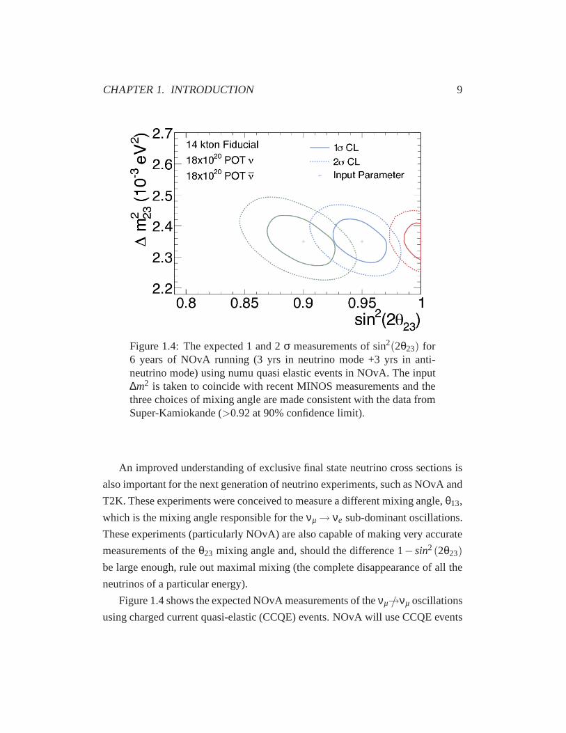
Figure 1.4: The expected 1 and 2σ measurements of sin2(2θ23) for6 years of NOvA running (3 yrs in neutrino mode +3 yrs in anti-neutrino mode) using numu quasi elastic events in NOvA. The input∆m2 is taken to coincide with recent MINOS measurements and thethree choices of mixing angle are made consistent with the data fromSuper-Kamiokande (>0.92 at 90% confidence limit).
An improved understanding of exclusive final state neutrinocross sections is
also important for the next generation of neutrino experiments, such as NOvA and
T2K. These experiments were conceived to measure a different mixing angle,θ13,
which is the mixing angle responsible for theνµ → νe sub-dominant oscillations.
These experiments (particularly NOvA) are also capable of making very accurate
measurements of theθ23 mixing angle and, should the difference 1−sin2(2θ23)
be large enough, rule out maximal mixing (the complete disappearance of all the
neutrinos of a particular energy).
Figure 1.4 shows the expected NOvA measurements of theνµ /→νµ oscillations
using charged current quasi-elastic (CCQE) events. NOvA will use CCQE events

CHAPTER 1. INTRODUCTION 10
because NOvA will have much better statistics than MINOS did, and using ex-
clusively CCQE events minimizes the effect of energy resolution smearing. How-
ever because the current generation of neutrino generatorsdo not contain SRCs
or MECs, and the signature of these multi-nucleon interactions is the presence of
additional low energy particles in the final state, it is possible that these poten-
tially below detection threshold low energy particles may introduce a significant
bias into the measurement of the oscillation parameters. Thus, in order to be fully
confident in the NOvA measurement of theνµ /→νµ oscillations, it is necessary to
have a full understanding of the impact of the multi-nucleoninteractions on the
CCQE cross section.

Chapter 2
Theory of the Weak Interaction
2.1 Weak Interaction Phenomenology
2.1.1 Fermi’s Point-like Four-Fermion Theory of β-Decay
It took four years from when Wolfgang Pauli first proposed theexistence of the
neutrino with his “Dear Radioactive Ladies and Gentlemen” letter [1] for a full
quantum field theory (QFT) of the weak interaction to be developed. The first
QFT of the weak interaction, proposed by Enrico Fermi, considered the electron-
neutrino pair emitted in the neutron to proton nuclear transition (n → p+ e+
ν) to be analagous to the emission of photons in nuclearγ-decay. Inspired by
quantum electrodynamics (QED), Fermi treated the interaction as happening at
one spacetime point. The interaction involved a 4-vector weak current between
the neutron and the proton. In addition, to ensure that the interaction would be
Lorentz invariant, Fermi included an additional current between the electron and
the neutrino, finally Fermi constructed a ‘current-current’ interaction amplitude:
GF√2
upγµunue−γµuν =GF√
2jµN jµl (2.1)
11
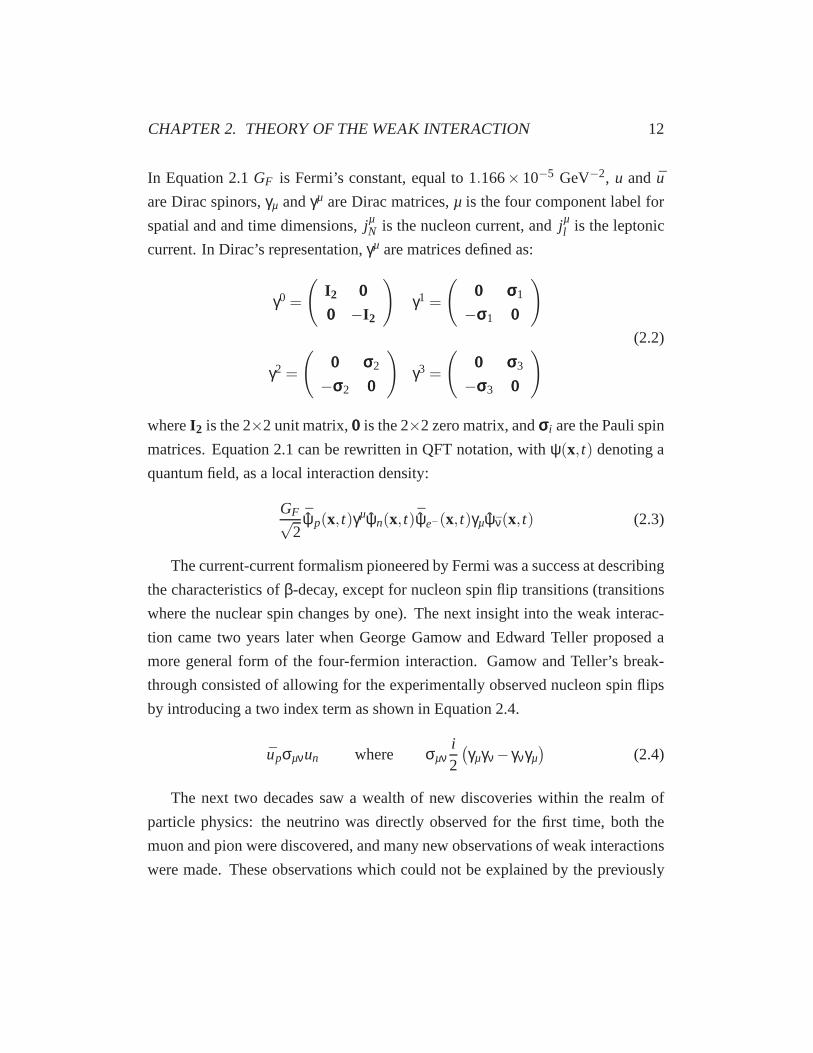
CHAPTER 2. THEORY OF THE WEAK INTERACTION 12
In Equation 2.1GF is Fermi’s constant, equal to 1.166×10⁻⁵ GeV−2, u and u
are Dirac spinors,γµ andγµ are Dirac matrices,µ is the four component label for
spatial and and time dimensions,jµN is the nucleon current, andjµl is the leptonic
current. In Dirac’s representation,γµ are matrices defined as:
γ0 =
(
I2 000
000 −I2
)
γ1 =
(
000 σσσ1
−σσσ1 000
)
γ2 =
(
000 σσσ2
−σσσ2 000
)
γ3 =
(
000 σσσ3
−σσσ3 000
)
(2.2)
whereI2 is the 2×2 unit matrix, 000 is the 2×2 zero matrix, andσσσi are the Pauli spin
matrices. Equation 2.1 can be rewritten in QFT notation, with ψ(x, t) denoting a
quantum field, as a local interaction density:
GF√2
¯ψp(x, t)γµψn(x, t) ¯ψe−(x, t)γµψν(x, t) (2.3)
The current-current formalism pioneered by Fermi was a success at describing
the characteristics ofβ-decay, except for nucleon spin flip transitions (transitions
where the nuclear spin changes by one). The next insight intothe weak interac-
tion came two years later when George Gamow and Edward Tellerproposed a
more general form of the four-fermion interaction. Gamow and Teller’s break-
through consisted of allowing for the experimentally observed nucleon spin flips
by introducing a two index term as shown in Equation 2.4.
upσµνun where σµνi2
(
γµγν −γνγµ)
(2.4)
The next two decades saw a wealth of new discoveries within the realm of
particle physics: the neutrino was directly observed for the first time, both the
muon and pion were discovered, and many new observations of weak interactions
were made. These observations which could not be explained by the previously
CHAPTER 2. THEORY OF THE WEAK INTERACTION 13
proposed theoretical forms of the weak interaction. The solution, first proposed by
Lee and Yang [15], called into doubt the conservation of parity (mirror symmetry)
in weak interactions. Much later it was determined that the weak interactions
maximally violates parity conservation, but this idea was very radical at the time.
2.1.2 The Axial Vector Structure of the Weak Interaction
Parity is an inversion of spatial coordinates, like a reflection in a mirror. Parity
allows for several definitions of physical quantities, polar vectors, axial vectors,
scalars, and pseudoscalars. A polar vector,V, is a vector that transforms in the
same way as the coordinatex under the parity operator,P:
P : x →−x , P : V →−V (2.5)
polar vector examples from introductory physics are quantities such as velocity,
momentum, and electric current. Axial vectors transform inthe same was as the
cross product of two polar vectors. There is no sign change under the parity
operator of axial vectors as shown in Equation 2.6.
P : U×V → (−U)× (−V) = U×V , P : A → A (2.6)
angular momentum, and spin are both examples of axial vectors. Scalars do not
change sign under the parity operator, this can be demonstrated by performing the
parity operator on the dot product of two polar vectors as shown in Equation 2.7.
P : U ·V → (−U) · (−V) = U ·V (2.7)
Pseudoscalars, however do change sign under the parity operator. Pseudoscalars
can be formed from the triple scalar product of three polar vectors as shown in
Equation 2.8.
P : U · (V ×W) → (−U) · (V ×W) (2.8)

CHAPTER 2. THEORY OF THE WEAK INTERACTION 14
It can be shown that the free particle solution to the Dirac equation of definite
parity is:
ψ(x, t) = N
(
φσσσ·p
E+mφ
)
e−iEt+ip·x (2.9)
whereφ is a two component Dirac spinor andN is a normalisation factor. Equa-
tion 2.9 transforms thusly under the parity operator:
P : ψ(x, t)→ ψP(x, t) = γ0ψ(−x, t) (2.10)
Thus a unitary quantum field operator,P can be defined such that:
ψP(x, t) = Pψ(x, t)P−1 = γ0ψ(−x, t) (2.11)
Using Equation 2.11 it becomes possible to consider the effects of the parity op-
erator on the previous forms of the weak interaction. As an example consider the
spatial part of Fermi’s weak 4-vector current:
ˆψ1P (x, t)γµψ2P (x, t) = ψ†1P (x, t)γ0γµψ2P (x, t)
= ψ†1(−x, t)γ0γ0γµγ0ψ2(−x, t)
= −ψ1(−x, t)γµψ2(−x, t) (2.12)
where γ0γµ = −γµγ0 and(
γ0)2= 1
Equation 2.12 shows that the spatial components of the 4-vector current trans-
form as a polar vector under the parity operator. Similarly the time component of
Fermi’s 4-vector current transforms as a scalar under the parity operator. Thus the
4-vector current of Fermi’s initial theory of the weak interaction does not allow
for the violation of parity. An extension of the theory must be made to allow for
parity violation. Parity violation can be accommodated by introducing terms that
CHAPTER 2. THEORY OF THE WEAK INTERACTION 15
transform as axial vectors. This is done using theγ5 matrix defined as:
γ5 = iγ0γ1γ2γ3 and{
γ5,γµ}
= 0 for µ∈ {0,1,2,3} (2.13)
It can be shown that a current withγ5 transforms as a pseudoscalar under the parity
operator. Thus a weak current that includesγ5 allows for parity violation in the
weak interaction. This is illustrated by Equation 2.14.
ˆψ1P (x, t)γ5ψ2P (x, t) = ψ†1P (x, t)γ0γ5ψ2P (x, t)
= ψ†1(−x, t)γ0γ0γ5γ0ψ2(−x, t) (2.14)
= −ψ1(−x, t)γ5ψ2(−x, t) where γ0γ5 = −γ5γ0
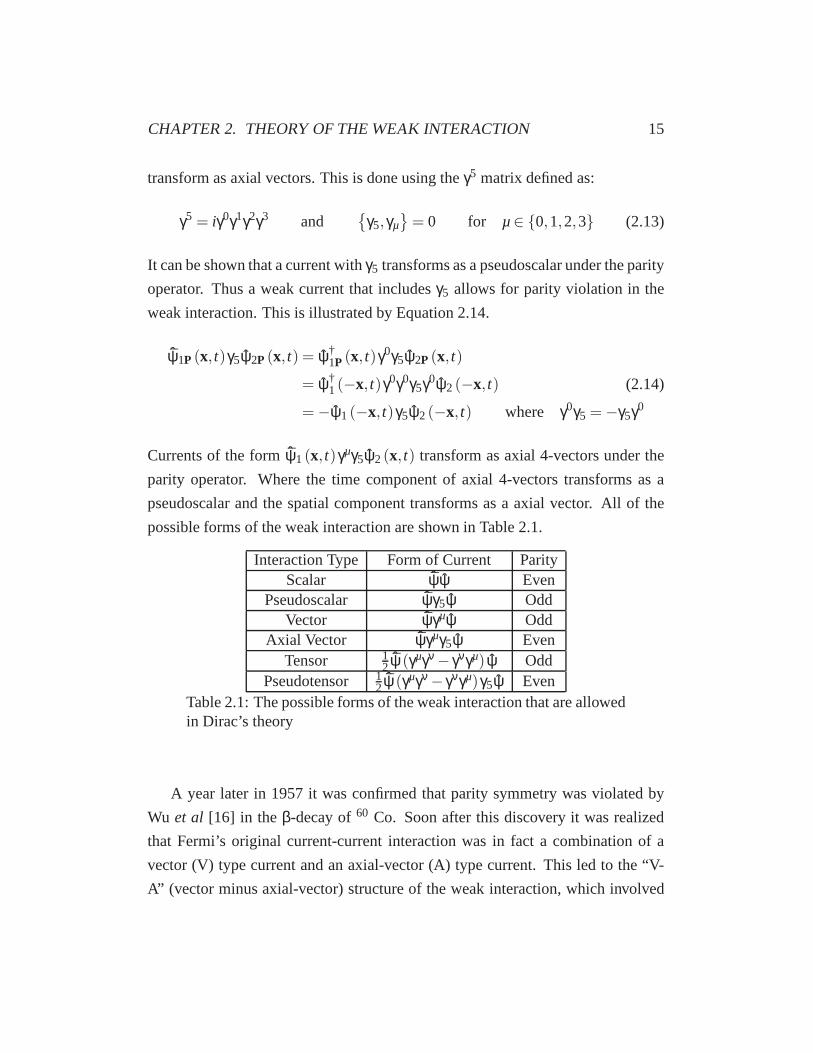
Currents of the formψ1(x, t)γµγ5ψ2(x, t) transform as axial 4-vectors under the
parity operator. Where the time component of axial 4-vectors transforms as a
pseudoscalar and the spatial component transforms as a axial vector. All of the
possible forms of the weak interaction are shown in Table 2.1.
Interaction Type Form of Current ParityScalar ˆψψ Even
Pseudoscalar ˆψγ5ψ OddVector ˆψγµψ Odd
Axial Vector ˆψγµγ5ψ EvenTensor 1
2ˆψ(γµγν −γνγµ)ψ Odd
Pseudotensor 12
ˆψ(γµγν −γνγµ)γ5ψ EvenTable 2.1: The possible forms of the weak interaction that are allowedin Dirac’s theory
A year later in 1957 it was confirmed that parity symmetry was violated by
Wu et al [16] in theβ-decay of60 Co. Soon after this discovery it was realized
that Fermi’s original current-current interaction was in fact a combination of a
vector (V) type current and an axial-vector (A) type current. This led to the “V-
A” (vector minus axial-vector) structure of the weak interaction, which involved

CHAPTER 2. THEORY OF THE WEAK INTERACTION 16
changing the original 4-vector current from Fermi to:
ue−γµuν → ue−γµ(1−γ5)uν (2.15)
This V-A structure of the weak interaction is a fundamental part of the Standard
Model. It has important implications for the way the left-handed (spin opposite the
direction of motion) vs. right-handed (spin in the direction of motion) components
of fermions (such as the neutrino) participate in the weak interaction.
2.1.3 Helicity and Chirality
The projection of the spin of a particle in the direction of the particles motion is
called the particles helicity. Thus the helicity operator is:
h =12
σσσ · p where p =p|p| (2.16)
Chirality is the sign of the helicity operator. Chirality isfundamental to the weak
interaction. Left-handed particles have negative chirality and right-handed parti-
cles have positive chirality. In the Pauli-Dirac representation of theγ matrices the
γ5 matrix is:
γ5 =
(
0 I2
I2 0
)
(2.17)
Applying theγ5 operator to the spinor solutions from Equation 2.9 yields:
γ5
(
ua
ub
)
=
(
0 I2
I2 0
)(
φσσσ·p
E+mφ
)
=
(
σσσ·pE+mφ
φ
)
(2.18)
Applying the relativistic approximation (E → |p| asm→ 0) gives:
γ5
(
ua
ub
)
=
(
(σσσ · p)φφ
)
=
(
(σσσ · p)φ(σσσ · p)2φ
)
(2.19)
CHAPTER 2. THEORY OF THE WEAK INTERACTION 17
thus:
γ5
(
ua
ub
)
=
(
σσσ · p 0
0 σσσ · p
)(
ua
ub
)
(2.20)
Equation 2.20 reveals that theγ5 operator approaches the helicity operator as the
mass of a particle goes to zero. The neutrino is assumed to be massless within the
Standard Model and thus the neutrino’s helicity is the same as the neutrino’s chi-
rality. Left-handed chirality massive particles will havemostly left-handed helic-
ity (with some right-handed helicity) and right-handed chirality massive particles
will have mostly right-handed helicity (with some left-handed helicity). This give
the helicity projection operators:
PL ≡(
1−γ5
2
)
, PR ≡(
1+γ5
2
)
(2.21)
The helicity projection operators satisfy the following relations:
P2R = PR , P2
L = PL , PRPL = PLPR = 0 , PR+PL = 1 (2.22)
The left, and right handed components of the Dirac spinors can then be defined
as:
uL ≡ PLu , ur ≡ PRu (2.23)
which allows for the rewriting of the V-A current between fermionic Dirac spinors
as:
u1γµ1−γ5
2u2 = u1γµPLu2 = u1γµP2
Lu2
= u1γµPLu2L = u1PRγµu2L
= u†1PLγ0γµu2L = u1Lγµu2L (2.24)
Equation 2.24 demonstrates the V-A structure of the theory of weak interactions.
Equation 2.24 implies that only the left-handed component of the chirality of
fermions participates in the weak interaction. This can also be shown for right
CHAPTER 2. THEORY OF THE WEAK INTERACTION 18
handed chirality anti fermions. Additionally, because thehelicity operator trans-
forms as a pseudoscalar under parity, it can be shown that theV-A structure of
weak interactions also implies that all massive fermions have the positive helic-
ity component suppressed by a factor of orderm/E, and similarly the negative
helicity component of massive fermions is also suppressed by the same factor.
The Standard Model makes no prediction about the helicity ofneutrinos, how-
ever the neutrino was assumed to be massless, and thus would have to have either
fully positive helicity or fully negative helicity. In 1958capture of electrons on152Eu showed that the helicity of the emitted neutrinos was 100%negative (within
experimental uncertainties)[17]. This result gave strongevidence for the V-A de-
scription of weak interactions, and also gave strong confirmation for the massless
neutrino of the Standard Model.
2.1.4 Electroweak Gauge Theory
Though the V-A theory was quite successful at describing theweak interaction, it
still assumed a current-current interaction which caused alot of theoretical issues.
By the 1960s theoretical physicists were working on a gauge theory of the weak
interaction. A weak gauge theory would consist of the introduction of a weak
gauge symmetry group, and a corresponding intermediate vector boson field. The
vector boson field is needed to keep the Lagranian invariant under certain local
transformations. The weak gauge theory allowed for the unification of the weak
force with the electromagnetic force, then through spontaneous symmetry break-
ing and the Higgs mechanism, the intermediate particles aquired masses becoming
the Standard Model vector bosons: photon (γ), Z0 and W±.
The gauge theory of the weak interaction viewse−L andνeL as two states of the
same ‘particle’ under the charged current (CC) processes. Assuming the particles
e−L andνeL are different states of the same underlying particle suggests that this
pair transform as a doublet under some symmetry group, a similar transformation
property would also hold for the pairs,µ−L ↔ νµL, τ−L ↔ ντL. TheSU(2) group was
originally proposed as the weak interaction group by Glashow [18], then expanded
CHAPTER 2. THEORY OF THE WEAK INTERACTION 19
upon by Weinberg [19] and Salam [20].
The weak interaction group is usually labeledSU(2)L to denote the fact that
it is only the left-handed component of the fields that participate in the weak in-
teraction, and also to distinguish it from the standardSU(2) group. Within the
weak gauge theory the left-handed component of the fields that enter into the
weak interaction corresponds to transformations in the internal space of the weak
isospin. TheSU(2) group is an isomorphic group to theSO(3) group, thus these
transformations can be considered to be rotations in a three-dimensional weak
isospin-space.I andI3 are used to denote the quantum numbers of weak isospin,
which have the following assignments for the leptonic fields:
I =12
I3 = +1/2
I3 = −1/2
(
νe
e−
)
L
(
νµ
µ−
)
L
(
ντ
τ−
)
L
(2.25)
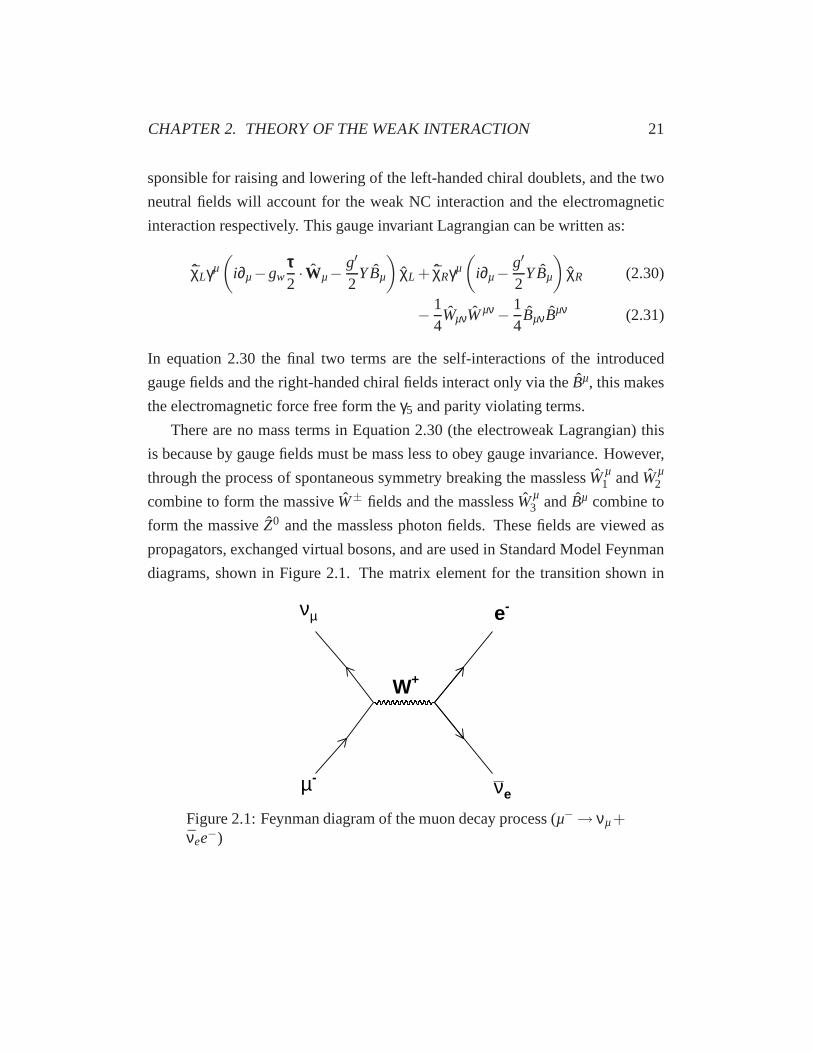
These transformations can be rewritten as:
(
νe
e−
)′
L
= e−i ααα·τττ2
(
νe
e−
)
L
(2.26)
whereτττ denotes Pauli spin matrices that act in the internal isospinspace. This
group should be considered as locally gauge invariant, thuslocal transformations
ααα (xµ) are allowed, without changing the observed physics. This group introduces
three gauge fields (one for each of the three axes in weak isospin-space); two of
the fields should have ‘charge’±1 and the third should be a neutral field. The
charged fields allow for transitions between the doublet members. The charged
fields corresponds to the charged current type interactionswhile the neutral field
corresponds to the neutral current (NC) interactions. NC interactions were first
observed in 1973 by the Gargamelle bubble chamber experiment at CERN [21]. It
was learned from the Gargamelle experiment that NC interactions are not pure V-
A, thus the neutral gauge field of the weak interaction, is notcompletely described
by the V-A theory of the weak interaction.

CHAPTER 2. THEORY OF THE WEAK INTERACTION 20
The proposed solution was the unification of the weak force with the electro-
magnetic force, this was done via the addition of an extraU(1) gauge group which
resulted in a newSU(2)L⊗U(1) structure for the unified electroweak force. The
new gauge group needed to include a mechanism to deal with theright-handed
electron (for electromagnetic interactions). Because theV-A structure works just
fine for CC weak interactions, this new mechanism needs to be asinglet in weak
isospin-space. As an example consider the first generation of leptons and quarks,
arranged into twoSU(2) doublets:
(
νe
e−
)
L
(
u
d
)
L
(2.27)
and threeSU(2) singlets;e−R, uR, dR. The weak hypercharge,Y, was introduced to
differentiate between left-handed doublet and right-handed singlet particles. The
weak hypercharge is defined as:
Y = 2Q−2I3 (2.28)
whereQ is the electric charge andI3 the third component of weak isospin. Both
the weak isospin and the local phase change fromt heU(1) transform should be lo-
cal gauge symmetries, thus local transformations should not change the observed
physics. This can be expressed as:
χ′L = exp
(
igwααα (xµ) · τττ
2+ ig′γ0(xµ)Y
)
χL (2.29)
whereχL is a left-handed chiral doublet,gw andg′ are coupling constants and
xµ is a space-time point. The Lagrangian must be kept invariantunder the local
SU(2)⊗U(1) transformation, this is done by introducing four new gauge fields;
two charged fields (Wµ1,2) and one neutral field (Wµ
3 ) for the SU(2) part of the
symmetry group, a second neutral field (Bµ) for theU(1) part of the symmetry
group. Just as in the V-A theory of weak interactions the charged fields are re-
CHAPTER 2. THEORY OF THE WEAK INTERACTION 21
sponsible for raising and lowering of the left-handed chiral doublets, and the two
neutral fields will account for the weak NC interaction and the electromagnetic
interaction respectively. This gauge invariant Lagrangian can be written as:
ˆχLγµ(
i∂µ−gwτττ2· Wµ−
g′
2YBµ
)
χL + ˆχRγµ(
i∂µ−g′
2YBµ
)
χR (2.30)
− 14WµνW
µν − 14
BµνBµν (2.31)
In equation 2.30 the final two terms are the self-interactions of the introduced
gauge fields and the right-handed chiral fields interact onlyvia theBµ, this makes
the electromagnetic force free form theγ5 and parity violating terms.
There are no mass terms in Equation 2.30 (the electroweak Lagrangian) this
is because by gauge fields must be mass less to obey gauge invariance. However,
through the process of spontaneous symmetry breaking the masslessWµ1 andWµ
2
combine to form the massiveW± fields and the masslessWµ3 andBµ combine to
form the massiveZ0 and the massless photon fields. These fields are viewed as
propagators, exchanged virtual bosons, and are used in Standard Model Feynman
diagrams, shown in Figure 2.1. The matrix element for the transition shown in
-µ
µν
+W
eν
-e
Figure 2.1: Feynman diagram of the muon decay process (µ− → νµ+νee−)
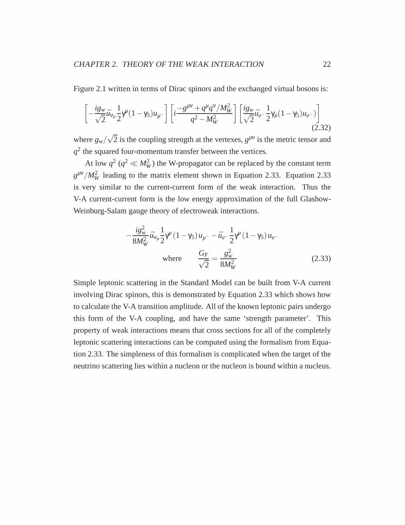
CHAPTER 2. THEORY OF THE WEAK INTERACTION 22
Figure 2.1 written in terms of Dirac spinors and the exchanged virtual bosons is:
[
− igw√2
uνµ
12
γµ(1−γ5)uµ−
][
i−gµν +qµqν/M2
W
q2−M2W
][
igw√2
ue−12
γµ(1−γ5)ue−)
]
(2.32)
wheregw/√
2 is the coupling strength at the vertexes,gµν is the metric tensor and
q2 the squared four-momentum transfer between the vertices.
At low q2 (q2 ≪ M2W) the W-propagator can be replaced by the constant term
gµν/M2W leading to the matrix element shown in Equation 2.33. Equation 2.33
is very similar to the current-current form of the weak interaction. Thus the
V-A current-current form is the low energy approximation ofthe full Glashow-
Weinburg-Salam gauge theory of electroweak interactions.
− ig2w
8M2W
uνµ
12
γµ(1−γ5)uµ− − ue−12
γµ(1−γ5)ue−
whereGF√
2=
g2w
8M2W
(2.33)
Simple leptonic scattering in the Standard Model can be built from V-A current
involving Dirac spinors, this is demonstrated by Equation 2.33 which shows how
to calculate the V-A transition amplitude. All of the known leptonic pairs undergo
this form of the V-A coupling, and have the same ‘strength parameter’. This
property of weak interactions means that cross sections forall of the completely
leptonic scattering interactions can be computed using theformalism from Equa-
tion 2.33. The simpleness of this formalism is complicated when the target of the
neutrino scattering lies within a nucleon or the nucleon is bound within a nucleus.
CHAPTER 2. THEORY OF THE WEAK INTERACTION 23
2.2 Neutrino-Nucleus Scattering
2.2.1 Neutrino Scattering Off of Nucleons
When the momentum transferred by the weak boson is low (q2 ≪ M2W), the pure
V-A description of weak interactions is a valid approximation. Even though the
previous discussion of weak interactions only addressed the lepton sector, the V-A
structure is also a valid description of vertices with a weakcurrent between quarks
such as:
uuγµ(1−γ5)ud (2.34)
Complications arise when going from the vertices involvinglone quarks to ver-
tices involving multiple quarks bound together in a nucleon, however. When con-
sidering neutrino scattering off of nucleons, it is important to consider additional
strong interaction effects. Unlike the leptons (and quarks), the nucleons (proton
and neutron) cannot be described as point like particles, consequently the inter-
nal structure of the nucleons must be included in any description of scattering
off of nucleons. Describing the effects of the nucleon internal structure involves
the use of quantum chromodynamics (QCD). QCD allows for manyadditional
processes such as quark-antiquark pair production from gluons and gluon emis-
sion from valence quarks. Even with these additional complications from QCD
the total electric charge must be always be conserved (the proton always has a
charge ofe), however there is no reason to assume this is also true for the weak
interaction. As an example, consider the formation of quark-antiquark pair, the
net contribution to the weak interaction from this quark-antiquark pair may not be
zero.
Ignoring for a moment intermediate vector bosons andq2 considerations, the
strong interaction effects can be accounted for by making the following replace-
ment in the weak current:
(1−γ5) → (cV −cAγ5) (2.35)

CHAPTER 2. THEORY OF THE WEAK INTERACTION 24
HerecV andcA are experimentally determined correction factors. These correction
factors have been measured throughβ-decay experiments to be:
cV = 1.000±0.003 , cA = 1.26±0.02 (2.36)
Equation 2.36 demonstrates that the vector part of the weak current is not modi-
fied by the QCD structure of the nucleon. This indicates that there may be some
conservation law that ‘protects’ the vector current in the same way that the elec-
tromagnetic charge is protected. This conservation law is known as the Conserved
Vector Current (CVC) hypothesis, which was first proposed byFeynman and Gell-
Mann [22]. They speculated that the vector part of the weak current upγµun, its
conjugate current ¯unγµup, and the electromagnetic current ¯upγµup form a triplet of
conserved currents in the internal isospin space of the strong interaction.
2.2.2 Neutrino-Nucleon Scattering Kinematics
It will be easier to discuss the theory of neutrino-nucleon scattering by first ad-
dressing the general kinematic quantities of CC neutrino-nucleon scattering. Fig-
ure 2.2 shows a diagram for the scattering processνµ + N → µ− + X (hereX
represents the hadronic final state). Figure 2.2 labels the measured quantities for
an event detected using in the MINOS detectors and the centerof mass frame
four-momentum of the particles in the interaction.
Table 2.2 lists how to calculate the Lorentz invariant kinematic quantities that
describe a general CCνµ−N interaction. The calculations are shown for both
the center of momentum frame (using four-momentum quantities), and for the lab
frame (detector measured quantities).
In quasi-elastic scattering (QE) event,νµ + n → µ− + p, the neutrino is con-
sidered to scatter off of the entire nucleon, and not the individual partons. In a
QE interaction the target nucleus does not break up but is just modified. If an in-
teraction is considered to be quasi-elastic then the hadronic system will consist of
a single proton (W2 = M2proton). QE scattering can be contrasted with resonances
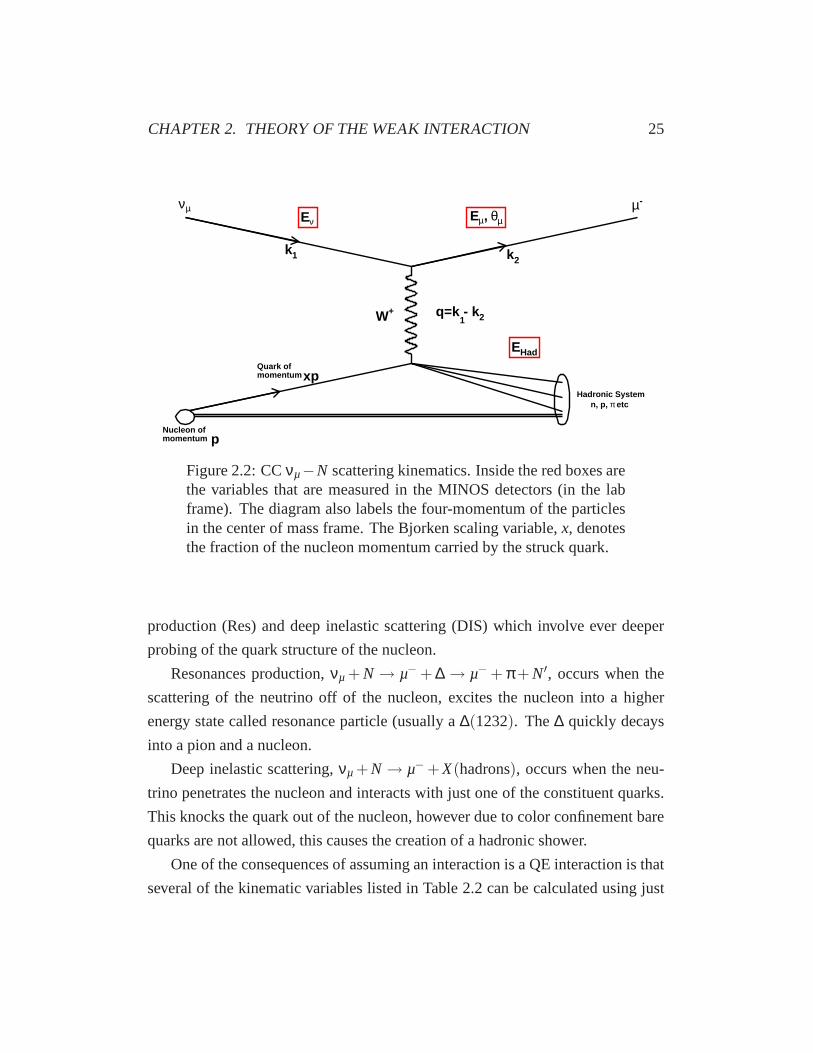
CHAPTER 2. THEORY OF THE WEAK INTERACTION 25
momentumNucleon of
p
νE µθ, µEµν
+W 2- k1
q=k
1k2k
momentumQuark of
xp
etcπ n, p, Hadronic System
HadE
-µ
Figure 2.2: CCνµ−N scattering kinematics. Inside the red boxes arethe variables that are measured in the MINOS detectors (in the labframe). The diagram also labels the four-momentum of the particlesin the center of mass frame. The Bjorken scaling variable,x, denotesthe fraction of the nucleon momentum carried by the struck quark.
production (Res) and deep inelastic scattering (DIS) whichinvolve ever deeper
probing of the quark structure of the nucleon.
Resonances production,νµ + N → µ− + ∆ → µ− + π+ N′, occurs when the
scattering of the neutrino off of the nucleon, excites the nucleon into a higher
energy state called resonance particle (usually a∆(1232). The∆ quickly decays
into a pion and a nucleon.
Deep inelastic scattering,νµ + N → µ− + X(hadrons), occurs when the neu-
trino penetrates the nucleon and interacts with just one of the constituent quarks.
This knocks the quark out of the nucleon, however due to colorconfinement bare
quarks are not allowed, this causes the creation of a hadronic shower.
One of the consequences of assuming an interaction is a QE interaction is that
several of the kinematic variables listed in Table 2.2 can becalculated using just

CHAPTER 2. THEORY OF THE WEAK INTERACTION 26
Variable Description Center of Momentum Lab FrameFrame Calculation Calculation
Energy transfered to ppp ·qqq/M Ehad
the hadronic system:νInelasticity:y (ppp ·qqq)/(ppp ·kkk1) Ehad/Eν
Squared four-momentum −qqq2 2EνEµ(
1−cos(
θµ))
transfer:Q2
Bjorken scaling variable:x Q2/2ppp ·qqq Q2/2EhadMSquared invariant mass of (ppp+qqq)2 M2+2EhadM−Q2
of the hadronic system:W2
Table 2.2: Lorentz invariant kinematic variables that describe thecharged current neutrino-nucleon scattering. The massM is the massof the struck nucleon.
the measured quantities that correspond to the outgoing muon. The QE-assumed
kinematic quantities introduced here along with the quantities in Table 2.2 will be
used extensively in the rest of this thesis.
• Neutrino Energy: In MINOS the usual way to reconstruct the neutrino
energy is by summing the visible energy in the detector for a given event,
Eν = Eµ+Ehad, whereEhad is calculated from the sum of the visible energy
not originated from the muon. However if an event is assumed to be due
to a QE interaction then a QE-assumed neutrino energy can be calculated
instead. This neutrino energy can be calculated using just the measured
muon kinematics according to:
EQEν =
EµM−(
M2µ
)
M−Eµ+ pµcos(
θµ) (2.37)
hereM is the mass of the struck nucleon,Mµ is the mass of the out going
muon. Equation 2.37 neglects terms involving the binding energy of the
struck nucleon.

CHAPTER 2. THEORY OF THE WEAK INTERACTION 27
• Squared four-momentum transfer: The QE-assumed four-momentum trans-
fer from the lepton to the hadronic system, it can also be calculated using
just the outgoing muon kinematics from:
Q2QE = −2EQE
ν(
Eµ− pµcos(
θµ))
+M2µ (2.38)
2.2.3 Nucleon Form Factors and the QE Cross Section
A νµ-CC QE scattering interaction can be described by:
νµ(p)+n(P) → µ−(
p′)
+ p(
P′) (2.39)
wherep (p′) is the incoming (outgoing) momentum of the lepton andP (P′) is
the incoming (outgoing) momentum of the nucleon. The Feynman diagram for
this interaction is shown in Figure 2.3. The matrix element for this interaction
n
µν
+W
p
-µ
Figure 2.3: Feynman diagram of theνµ-CC QE interaction, showingboth theνµ, W+, µ− and then, W+, p vertices.
can be calculated by modifying Equation 2.33 using equation2.34 then including
the further effects of having the quarks bound within a nucleon. This is given in
CHAPTER 2. THEORY OF THE WEAK INTERACTION 28
Equation 2.40:
GF√2
¯uµ−(
p′)
γµ(1−γ5)uνµ (p)cos(θC) up(
P′)ΓµCC
(
q2)un(P) (2.40)
whereθC is the Cabibbo angle (which measures the probability of quark flavor
change due to the weak interaction [23] [24]) andΓµCC
(
q2)
is a term that contains
the complex weak nucleon form factors given by Equation 2.41:
ΓµCC = γµF2
V
(
q2)+iσµνqν
2MξF2
V
(
q2)+qµ
MFS(
q2)
+
(
γµFA(
q2)+iσµνqν
2MFT(
q2)+qµ
MFP(
q2))
γ5 (2.41)
whereM is the mass of the struck nucleon. Each term inΓµCC is a form fac-
tor that parameterizes the amount of each type of weak current participating the
interaction. The form factors are functions of the vector boson ‘probe’ squared
four-momentum,q2, which reflects the fact that the vector boson interacts with
the nucleon internal structure at different ‘levels’ depending on the bosonsq2.
These form factors are related to the correction factors of Equation 2.35,cV and
cA, in theq2 = 0 limit.
Whereξ = kp− kn + 1, with kp/kn being the anomalous magnetic moments
of the proton and neutron. Examining Table 2.1 the V-type nucleon from factors
are: the vector form factorsF1V , F2
V , and the scalar form factorFS (which doesn’t
contribute to the weak interaction). In the standard model the A-type nucleon
form factors are: the axial-vector form factorFA, the pseudotensor form factor
FT (which doesn’t contribute to the weak interaction), and thepseudoscalar form
factorFP.
Llewellyn-Smith explained why the nucleon form factors must be real. In [25],
Llewellyn-Smith pointed out that time reversal symmetry (T) requires that, all of
the nucleon form factors must be real and charge-exchange symmetry (C) requires
CHAPTER 2. THEORY OF THE WEAK INTERACTION 29
FS, andFT to be imaginary. ThusFS, andFT must be zero:
FS(
q2)= FT(
q2)= 0 ∀q2 (2.42)
The muon mass multiplies the nucleon form factorFP, thus for neutrino en-
ergies wherem2µ ≪ E2
ν the pseudoscalar from factor can be neglected. SettingFS
andFT equal to 0 and neglecting the pseudoscalar form factor turnsEquation 2.41
into:
ΓµCC = γµ(FV
(
q2)−γ5FA(
q2))+iσµνqµ
2MξF2
V
(
q2) (2.43)
Inserting Equation 2.43 into Equation 2.40 yields the full expression for the matrix
element:
GF√2
¯uµ−(
p′)
γµ(1−γ5)uνµ (p)cos(θC) up(
P′)(
γµ(F1V
(
q2)−γ5FA(
q2))
+iσµνqν
2MξF2
V
(
q2))
un(P) (2.44)
Turning the reduced form of the matrix element (Equation 2.44) into a differential
cross section with respect toq2, for QE scattering yields Equations 2.45 and 2.46.
dσd |q2| =
M2G2Fcos2(θc)
8πE2ν
[
A(
q2)−B(
q2) s−uM2 +C
(
q2) (s−u)2
M4
]
(2.45)
dσd |q2| =
M2G2Fcos2(θc)
8πE2ν
[
A(
q2)+B(
q2) s−uM2 +C
(
q2) (s−u)2
M4
]
(2.46)
where Equation 2.45 is for the interactionν + n → l− + p, and Equation 2.46 is
for the interactionν+ p→ l−+n. In Equations 2.45 and 2.46s−u= EνM−q2−m2
l , ml is the mass of the outgoing lepton and theA(
q2)
, B(
q2)
, C(
q2)
can be
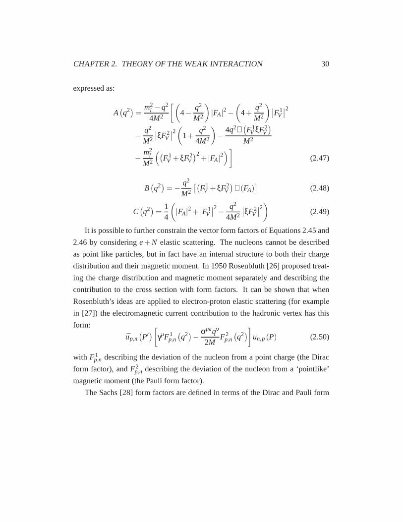
CHAPTER 2. THEORY OF THE WEAK INTERACTION 30
expressed as:
A(
q2)=m2
l −q2
4M2
[(
4− q2
M2
)
|FA|2−(
4+q2
M2
)
∣
∣F1V
∣
∣
2
− q2
M2
∣
∣ξF2V
∣
∣
2(
1+q2
4M2
)
− 4q2ℜ(
F1V ξF2
V
)
M2
− m2l
M2
(
(
F1V + ξF2
V
)2+ |FA|2
)
]
(2.47)
B(
q2)= − q2
M2
[(
F1V + ξF2
V
)
ℜ (FA)]
(2.48)
C(
q2)=14
(
|FA|2+∣
∣F1V
∣
∣
2− q2
4M2
∣
∣ξF2V
∣
∣
2)
(2.49)
It is possible to further constrain the vector form factors of Equations 2.45 and
2.46 by consideringe+ N elastic scattering. The nucleons cannot be described
as point like particles, but in fact have an internal structure to both their charge
distribution and their magnetic moment. In 1950 Rosenbluth[26] proposed treat-
ing the charge distribution and magnetic moment separatelyand describing the
contribution to the cross section with form factors. It can be shown that when
Rosenbluth’s ideas are applied to electron-proton elasticscattering (for example
in [27]) the electromagnetic current contribution to the hadronic vertex has this
form:
up,n(
P′)[
γµF1p,n
(
q2)− σµνqν
2MF2
p,n
(
q2)]
un,p(P) (2.50)
with F1p,n describing the deviation of the nucleon from a point charge (the Dirac
form factor), andF2p,n describing the deviation of the nucleon from a ‘pointlike’
magnetic moment (the Pauli form factor).
The Sachs [28] form factors are defined in terms of the Dirac and Pauli form
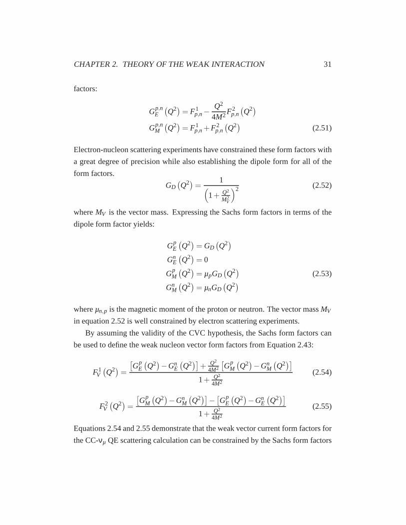
CHAPTER 2. THEORY OF THE WEAK INTERACTION 31
factors:
Gp,nE
(
Q2)= F1p,n−
Q2
4M2F2p,n
(
Q2)
Gp,nM
(
Q2)= F1p,n+F2
p,n
(
Q2) (2.51)
Electron-nucleon scattering experiments have constrained these form factors with
a great degree of precision while also establishing the dipole form for all of the
form factors.
GD(
Q2)=1
(
1+ Q2
M2V
)2 (2.52)
whereMV is the vector mass. Expressing the Sachs form factors in terms of the
dipole form factor yields:
GpE
(
Q2)= GD(
Q2)
GnE
(
Q2)= 0
GpM
(
Q2)= µpGD(
Q2) (2.53)
GnM
(
Q2)= µnGD(
Q2)
whereµn,p is the magnetic moment of the proton or neutron. The vector massMV
in equation 2.52 is well constrained by electron scatteringexperiments.
By assuming the validity of the CVC hypothesis, the Sachs form factors can
be used to define the weak nucleon vector form factors from Equation 2.43:
F1V
(
Q2)=
[
GpE
(
Q2)
−GnE
(
Q2)]
+ Q2
4M2
[
GpM
(
Q2)
−GnM
(
Q2)]
1+ Q2
4M2
(2.54)
F2V
(
Q2)=
[
GpM
(
Q2)
−GnM
(
Q2)]
−[
GpE
(
Q2)
−GnE
(
Q2)]
1+ Q2
4M2
(2.55)
Equations 2.54 and 2.55 demonstrate that the weak vector current form factors for
the CC-νµ QE scattering calculation can be constrained by the Sachs form factors
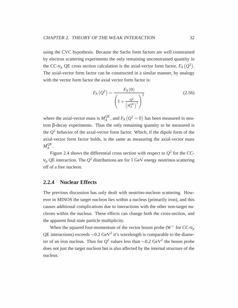
CHAPTER 2. THEORY OF THE WEAK INTERACTION 32
using the CVC hypothesis. Because the Sachs form factors arewell constrained
by electron scattering experiments the only remaining unconstrained quantity in
the CC-νµ QE cross section calculation is the axial-vector form factor, FA(
Q2)
.
The axial-vector form factor can be constructed in a similarmanner, by analogy
with the vector form factor the axial vector form factor is:
FA(
Q2)=FA(0)
(
1+ Q2(
MQEA
)2
)2 (2.56)
where the axial-vector mass isMQEA , andFA
(
Q2 = 0)
has been measured in neu-
tron β-decay experiments. Thus the only remaining quantity to be measured is
theQ2 behavior of the axial-vector form factor. Which, if the dipole form of the
axial-vector form factor holds, is the same as measuring theaxial-vector mass
MQEA .
Figure 2.4 shows the differential cross section with respect to Q2 for the CC-
νµ QE interaction. TheQ2 distributions are for 1 GeV energy neutrinos scattering
off of a free nucleon.
2.2.4 Nuclear Effects
The previous discussion has only dealt with neutrino-nucleon scattering. How-
ever in MINOS the target nucleon lies within a nucleus (primarily iron), and this
causes additional complications due to interactions with the other non-target nu-
cleons within the nucleus. These effects can change both thecross-section, and
the apparent final state particle multiplicity.
When the squared four-momentum of the vector boson probe (W+ for CC-νµ
QE interactions) exceeds∼0.2 GeV2 it’s wavelength is comparable to the diame-
ter of an iron nucleus. Thus forQ2 values less than∼0.2 GeV2 the boson probe
does not just the target nucleon but is also affected by the internal structure of the
nucleus.

CHAPTER 2. THEORY OF THE WEAK INTERACTION 33
2 (GeV/c)2 Q0 0.2 0.4 0.6 0.8 1 1.2
2 (
cm/G
eV)
-38
10
× 2/d
Qσ
d
0
0.2
0.4
0.6
0.8
1
1.2
1.4
1.6
1.8
2 =1.0AM
=1.1AM
=1.2AM
= 1.0 GeVνE
2 (GeV/c)2 Q0 0.2 0.4 0.6 0.8 1 1.2
=1.0
A N
orm
aliz
ed to
M2
/dQ
σ d
0
0.2
0.4
0.6
0.8
1
1.2
1.4
1.6
1.8
2 =1.0AM
=1.1AM
=1.2AM
= 1.0 GeVνE
Figure 2.4: Above: quasi-elastic differential cross section off of a freenucleon with respect toQ2. Each distribution corresponds to a differ-ent value of the axial-vector mass parameter. Below: The same Q2
distribution as above except the red and blue distributionsare normal-ized to the area of the blackQ2 distribution.
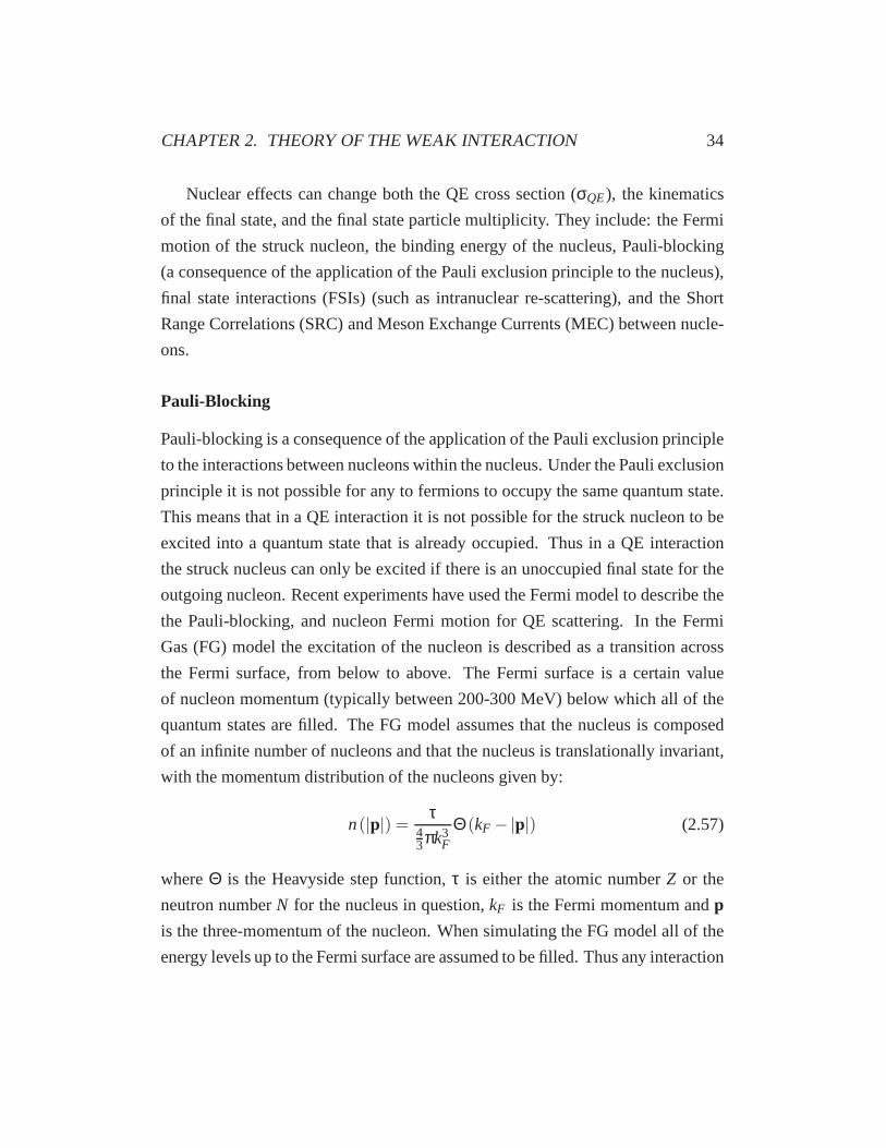
CHAPTER 2. THEORY OF THE WEAK INTERACTION 34
Nuclear effects can change both the QE cross section (σQE), the kinematics
of the final state, and the final state particle multiplicity.They include: the Fermi
motion of the struck nucleon, the binding energy of the nucleus, Pauli-blocking
(a consequence of the application of the Pauli exclusion principle to the nucleus),
final state interactions (FSIs) (such as intranuclear re-scattering), and the Short
Range Correlations (SRC) and Meson Exchange Currents (MEC)between nucle-
ons.
Pauli-Blocking
Pauli-blocking is a consequence of the application of the Pauli exclusion principle
to the interactions between nucleons within the nucleus. Under the Pauli exclusion
principle it is not possible for any to fermions to occupy thesame quantum state.
This means that in a QE interaction it is not possible for the struck nucleon to be
excited into a quantum state that is already occupied. Thus in a QE interaction
the struck nucleus can only be excited if there is an unoccupied final state for the
outgoing nucleon. Recent experiments have used the Fermi model to describe the
the Pauli-blocking, and nucleon Fermi motion for QE scattering. In the Fermi
Gas (FG) model the excitation of the nucleon is described as atransition across
the Fermi surface, from below to above. The Fermi surface is acertain value
of nucleon momentum (typically between 200-300 MeV) below which all of the
quantum states are filled. The FG model assumes that the nucleus is composed
of an infinite number of nucleons and that the nucleus is translationally invariant,
with the momentum distribution of the nucleons given by:
n(|p|) =τ
43πk3
F
Θ(kF −|p|) (2.57)
whereΘ is the Heavyside step function,τ is either the atomic numberZ or the
neutron numberN for the nucleus in question,kF is the Fermi momentum andp
is the three-momentum of the nucleon. When simulating the FGmodel all of the
energy levels up to the Fermi surface are assumed to be filled.Thus any interaction
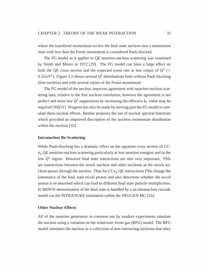
CHAPTER 2. THEORY OF THE WEAK INTERACTION 35
where the transfered momentum excites the final state nucleon into a momentum
state with less than the Fermi momentum is considered Pauli-blocked.
The FG model as it applies to QE neutrino-nucleus scatteringwas examined
by Smith and Moniz in 1972 [29]. The FG model can have a large effect on
both the QE cross section and the expected event rate at low values of Q2 (<
0.2GeV2). Figure 2.5 shows severalQ2 distributions both without Pauli blocking
(free nucleon) and with several values of the Fermi momentum.
The FG model of the nucleus improves agreement with neutrino-nucleus scat-
tering data, relative to the free nucleon simulation, however the agreement is not
perfect and more lowQ2 suppression by increasing the effectivekF value may be
required [30][31]. Progress has also be made by moving past the FG model to sim-
ulate these nuclear effects. Benhar proposes the use of nuclear spectral functions
which provided an improved description of the nucleon momentum distribution
within the nucleus [32].
Intranuclear Re-Scattering
While Pauli-blocking has a dramatic effect on the apparent cross section of CC-
νµ QE neutrino-nucleus scattering particularly at low neutrino energies and in the
low Q2 region. However final state interactions are also very important. FSIs
are interactions between the struck nucleon and other nucleons as the struck nu-
cleon passes through the nucleus. Thus for CCνµ QE interactions FSIs change the
kinematics of the final state recoil proton and also determine whether the recoil
proton is re-absorbed which can lead to different final stateparticle multiplicities.
In MINOS determination of the final state is handled by a an intranuclear cascade
model via the INTRANUKE simulation within the NEUGEN MC [33].
Other Nuclear Effects
All of the neutrino generators in common use by modern experiments simulate
the nucleus using a variation on the relativistic fermi gas (RFG) model. The RFG
model simulates the nucleus as a collection of non-interacting nucleons that obey
CHAPTER 2. THEORY OF THE WEAK INTERACTION 36
Figure 2.5: The CC-νµ QE differential cross section with respect toQ2 with several values ofkF compared to the free nucleon case, showsthe lowQ2 suppression characteristic of Pauli-blocking. Taken froma talk given by M. Sakuda at the 2005 NuFact conference.
Fermi-Dirac statistics. The RFG is a relatively simple model with physics that is
easy to calculate within an MC simulation. However the RFG model is an over
simplification of the nucleus because the nucleons do interact with each other.
Measurements of the CCQE cross-section over the last ten years have revealed
a 20-30% increase in both the value of the CCQE cross section and in the mea-
sured value ofMQEA , the only free parameter in the CCQE model. The global mean
for MQEA from early bubble chamber neutrino experiments is 1.02 ± 0.06 GeV.
Since then K2K, MiniBooNE, MINOS, and SciBooNE have all measuredMQEA
to be 20-30% higher, with only the NOMAD experiment measuring anMQEA that
is consistent with the earlier global mean. The early experiments used deuterium
as the nuclear target, while the more recent high statisticsexperiments have used
higher A targets: carbon (MiniBooNE, SciBooNE and NOMAD), oxygen (K2K),

CHAPTER 2. THEORY OF THE WEAK INTERACTION 37
and iron (MINOS). In these higher A targets, the non-interacting nucleon assump-
tion of the RFG may no longer be a useful.
0 0.1 0.2 0.3 0.4 0.5 0.6 0.7 0.8 0.9 1 1.1 1.2Eν [GeV]
0
2
4
6
8
10
12
14
16
σ/(A
-Z)
[10-3
9 cm
2 ]
MiniBooNEQE+np-nhQE
Figure 2.6: The MiniBooNEνµ CCQE cross section as a function ofthe incident neutrino energy. The points are the MiniBooNE data, thered line is theνµ CCQE cross section with anMQE
A value of 1.02 GeVand including the effect of the most important types of SRC interac-tions. The black dashed line is the sameνµ CCQE cross section with-out the SRT interactions. There is remarkable agreement between theMiniBooNE data and theQE+np−nh model. This agreement indi-cates that the 20-30% discrepancy in the recent high statistics interac-tion experiments could, in part, be due to these SRC type interactions.
The MiniBooNE experiment has measured theνµ CCQE cross section in a
manner that is largely model independent [34]. This cross section measurement
is consistent with anMQEA value of 1.35 GeV. This is more than 30% above the
global mean of 1.02 GeV. The MiniBooNE detector is a spherical container of
CHAPTER 2. THEORY OF THE WEAK INTERACTION 38
800 tons of mineral oil surrounded by 1280 photomultiplier tubes. MiniBooNE is
a Cherenkov detector so they are largely insensitive to the recoil proton of theνµ
CCQE interaction. They would also be insensitive to the secondary nucleon from
a CCQE-like SRC type interaction. M. Martiniet al. have calculated the CCQE
cross section with anMQEA value 1.02 GeV and including SRC [35]. As shown in
Figure 2.6 they find good agreement with the MiniBooNE data.

Chapter 3
Survey of Current Results
Electron scattering experiments have measured the nucleonvector form factors
(F1V andF2
V ), neutronβ-decay experiments have measured the axial-vector form
factor atQ2 = 0 (FA(
Q2 = 0)
. Both of these measurements have been made with
high precision. Only neutrino-nucleon scattering is sensitive to theQ2 dependence
of the axial-vector form factor (FA). Thus if the dipole form of the axial-vector
form factor is assumed then measurements of the CC-νµ QE cross section are
equivalent to measuring the axial-vector massMQEA .
3.1 Generalized Method for MeasuringMQEA
Fundamentally the dipole assumption for the axial-vector form factor is only
driven by the success of the dipole form in describing the vector form factors.
There is no underlying physical theory driving the choice ofthe dipole form, ex-
cept the success of the dipole form in describing the vector form factors. However
the use of the dipole form to describe the axial-vector form factor has several ad-
vantages, most prominent of which is the use of symbolic formwith a proven
track record that has only one free parameter.
The axial-vector form factor is the only quantity currentlynot well measured
within the theoretical framework describing neutrino-nucleon QE scattering (as
39

CHAPTER 3. SURVEY OF CURRENT RESULTS 40
given by Equation 2.45). When the axial-vector form factor is described using
the dipole approximation the only free parameter is the axial-vector mass (MQEA ).
Thus the way neutrino scattering experiments measure theMQEA parameter is by
examining (usually by fitting) theQ2 distribution for charged current QE interac-
tions.
Figure 2.4 from Section 2.2.3 shows how changes in theMQEA parameter re-
sults in changes to the CC-νµ QE Q2 spectrum. The upper plot in Figure 2.4
shows how changingMQEA changes the absolute cross section and the lower plot
in Figure 2.4 shows how changingMQEA changes the shape of theQ2 distribution
when normalization is ignored. Thus there are two possible ways to measure the
MQEA parameter using theQ2 spectrum of CCQE interactions. It is possible to
measureMQEA by examining the shape and rate information within the CCQEQ2
spectrum, or it is also possible to measureMQEA just by examining the shape of the
Q2 distribution.
3.2 Summary of World Average Values
Table 3.1 summarizes many previous measurement of the axial-vector massMQEA .
The weighted average forMQEA from neutrino-nuclei scattering experiments com-
piled in 2001 (deliberately chosen to exclude the modern high Z target experi-
ments) is 1.026±0.021 GeV.
When considering these measurements a number of factors areimportant to
fully understand the differences between the measurementsof the axial-vector
massMQEA , these include but are not limited to: the nuclear target, analysis method-
ology, neutrino flux uncertainties, background cross section uncertainties, the for-
malism used in describing the form factors, and the nuclear model used. Depend-
ing on the details of how the analysis addresses all of these factors, the eventual
measurement ofMQEA could be considered as an effective measurement of the
axial-vector mass, where other unknown physics are being absorbed into the mea-
surement of the axial-vector mass. The relative importanceof these factors are

CHAPTER 3. SURVEY OF CURRENT RESULTS 41
summarized below:
• Target Nucleus: The modeling uncertainty for higherZ nuclear targets is
largest in the lowQ2 region. Most of the previous measurement of the axial-
vector mass have used a lowQ2 cutoff. Most of the experiments that used
a low Q2 cutoff demonstrated consistency to small changes to this cutoff
value. It isn’t yet clear whetherMQEA , when treated as a effective parameter,
should be a constant for all nuclei, or if it has a Z dependence.
• Fit Methodology: There have been several different methods used to de-
termine the axial-vector mass used in previous analysis of CC-νµ QE data,
these methods include: rate only, shape only, rate and shape, flux indepen-
dent, fitting theQ2 distribution, fitting theQ2 distribution in slices ofEν,
and fitting theQ2 andEν distribution simultaneously. As more information
is included in the fit, the analysis becomes sensitive to a larger number of
uncertainties. The rate and shape method maximizes the available informa-
tion, thus the analysis would become more sensitive to uncertainties in the
background normalization and also uncertainties in the neutrino flux. Some
previous experiments have used multiple methods, those that have usually
find self-consistent values for the axial-vector mass.
• Flux Uncertainties: A significant number of the previous measurements
were unable to use rate information when extracting their value of the axial-
vector mass because they did not have sufficient knowledge ofthe incident
neutrino flux. These experiments would use the shape only or flux indepen-
dent methods to minimize the effect that their flux uncertainty had on their
measurement of the axial-vector mass. This is because theQ2 distribution
is not strongly dependent on the neutrino energy.
• Background Uncertainties: The deuterium bubble chamber experiments
(such as the ANL one discussed in Section 3.3.1) were able to achieve very
high QE purity, thus mostly eliminating the effect that uncertainties in the
CHAPTER 3. SURVEY OF CURRENT RESULTS 42
background cross section andQ2 distributions had on the final axial-vector
mass uncertainty. The dominant background for QE scattering is single pion
production (primarily from resonant particle decay). There is a correspond-
ing axial-vector mass for single pion productionMRESA (also calledM1π
A ).
When the QE selection has a lower purity of QE interactions the extracted
MQEA value could have an artificially high or low value due to this back-
ground contamination. Also correlations betweenMQEA andMRES
A will have
the effect of increasing the uncertainty in best fit QE axial-vector mass.
• Vector Form Factors: Previous measurements of the axial-vector mass
have assumed the dipole form for the nucleon weak vector formfactors.
However, recent work by Bodeket al [36] [37] suggests an alternate form
for these form factors. Because the extraction of the axial-vector mass is
sensitive to the choice of these vector form factors, and also to other pa-
rameters used in model of the nucleon (such asFA(
Q2 = 0)
), the choice of
global average could have an effect on the extracted axial-vector mass.
• Nuclear Model Used: Most neutrino experiments are using or have used
the RFG model to describe the behavior of the nucleus. It seems pretty clear
now that the RFG model is inadequate to describe the actual behavior of the
nucleus. Newer neutrino event generator MC (such as GENIE [38]) are
beginning to included improved models of Pauli-blocking such as nuclear
spectral functions. The treatment of Pauli-blocking is notthe only element
missing from neutrino event generators, as discussed in Sections 3.4, and
2.2.4, there are other nuclear effects due to correlations and interactions
between nucleons that are not considered in neutrino-nuclei scattering, but
appear to be more important that previously thought.
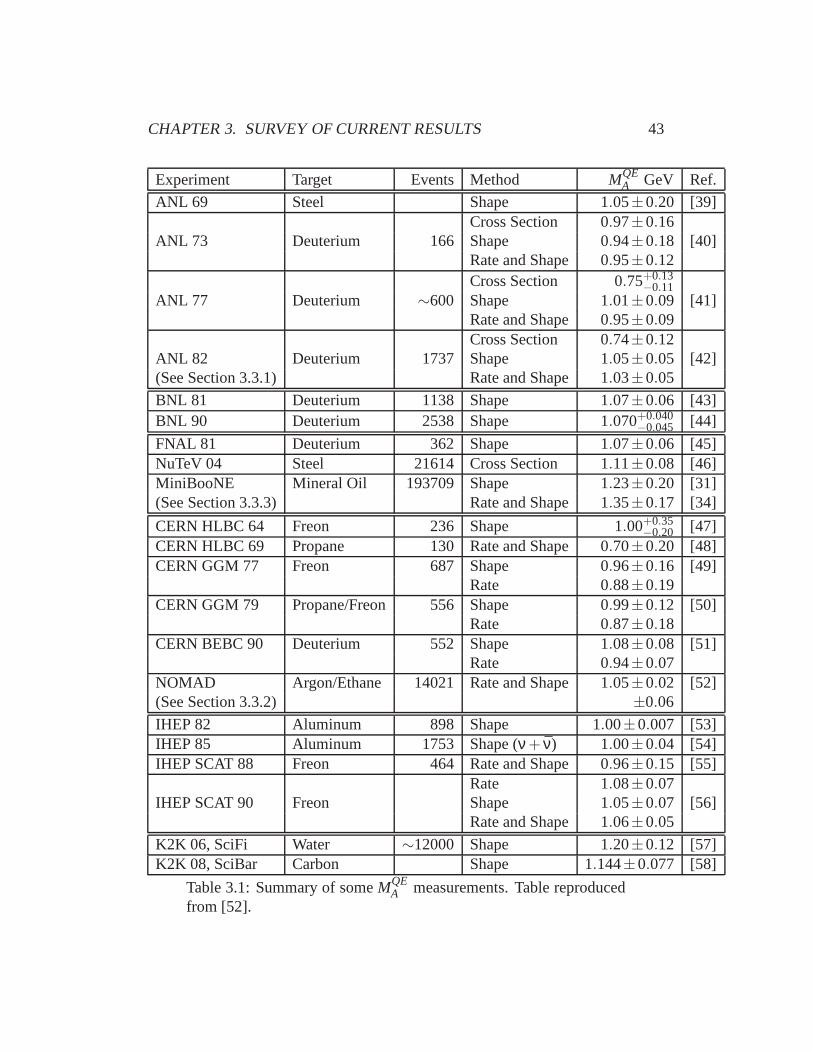
CHAPTER 3. SURVEY OF CURRENT RESULTS 43
Experiment Target Events Method MQEA GeV Ref.
ANL 69 Steel Shape 1.05±0.20 [39]Cross Section 0.97±0.16
ANL 73 Deuterium 166 Shape 0.94±0.18 [40]Rate and Shape 0.95±0.12Cross Section 0.75+0.13
−0.11ANL 77 Deuterium ∼600 Shape 1.01±0.09 [41]
Rate and Shape 0.95±0.09Cross Section 0.74±0.12
ANL 82 Deuterium 1737 Shape 1.05±0.05 [42](See Section 3.3.1) Rate and Shape 1.03±0.05
BNL 81 Deuterium 1138 Shape 1.07±0.06 [43]BNL 90 Deuterium 2538 Shape 1.070+0.040
−0.045 [44]
FNAL 81 Deuterium 362 Shape 1.07±0.06 [45]NuTeV 04 Steel 21614 Cross Section 1.11±0.08 [46]MiniBooNE Mineral Oil 193709 Shape 1.23±0.20 [31](See Section 3.3.3) Rate and Shape 1.35±0.17 [34]
CERN HLBC 64 Freon 236 Shape 1.00+0.35−0.20 [47]
CERN HLBC 69 Propane 130 Rate and Shape 0.70±0.20 [48]CERN GGM 77 Freon 687 Shape 0.96±0.16 [49]
Rate 0.88±0.19CERN GGM 79 Propane/Freon 556 Shape 0.99±0.12 [50]
Rate 0.87±0.18CERN BEBC 90 Deuterium 552 Shape 1.08±0.08 [51]
Rate 0.94±0.07NOMAD Argon/Ethane 14021 Rate and Shape 1.05±0.02 [52](See Section 3.3.2) ±0.06
IHEP 82 Aluminum 898 Shape 1.00±0.007 [53]IHEP 85 Aluminum 1753 Shape (ν + ν) 1.00±0.04 [54]IHEP SCAT 88 Freon 464 Rate and Shape 0.96±0.15 [55]
Rate 1.08±0.07IHEP SCAT 90 Freon Shape 1.05±0.07 [56]
Rate and Shape 1.06±0.05
K2K 06, SciFi Water ∼12000 Shape 1.20±0.12 [57]K2K 08, SciBar Carbon Shape 1.144±0.077 [58]
Table 3.1: Summary of someMQEA measurements. Table reproduced
from [52].
CHAPTER 3. SURVEY OF CURRENT RESULTS 44
3.3 Survey ofMQEA Measurements
Table 3.1 summarizes measured results for the quasi-elastic axial-vector mass
MQEA . What follows will be a more detailed look at a few of these publications.
These results are presented as ‘case-studies’ of the different ways thatMQEA can be
measured, while also exploring sources of some of the tension that is seen between
the earlier measurements and the more recent measurements.
3.3.1 Argonne 12-Foot Bubble Chamber
Argonne National Lab (ANL) has the honor of having made the most accurate
measurement ofMQEA . This measurement was made using the twelve foot bubble
chamber at ANL, which was exposed to a neutrino beam producedat the Zero
Gradient Synchrotron (ZGS) facility. The ZGS focused 12.4 GeV protons onto
a beryllium target, the resulting hadrons were focused by two magnetic horns.
The focused hadrons (mainlyπ+) were allowed to decay to intoµ+ andνµ, any
un-decayed hadrons and the charged leptons where absorbed by the steel and lead
absorber at the end of the 30m decay region. The remaining muon neutrinos would
pass through the absorber, this resulting beam of neutrinoswere incident on the
deuterium filled bubble chamber.
The resulting muon neutrino beam from the ZGS facility had a peak neutrino
energy of∼0.5 GeV with a tail that reached up to∼6 GeV. This neutrino beam was
modeled using a simulation of the neutrino beamline, the simulation was tuned
using the measured hadron production fromp-Bescattering. This constrained the
flux to an estimated uncertainty of±15% except in the high energy tail where a
significant fraction of the neutrino production came from kaon decays, here the
lack ofK+ production measurements increased the flux uncertainty to±25%.
The Argonne twelve foot bubble chamber was filed with liquid deuterium
that had been heated to just below the boiling point for deuterium. The pressure
within the bubble chamber was mechanically reduced in anticipation of particles
passing through the chamber. This lower pressure causes thedeuterium to en-

CHAPTER 3. SURVEY OF CURRENT RESULTS 45
ter a metastable superheated phase, thus when charged particles enter the cham-
ber the would leave an ionization trail. The ionization would cause bubbles to
form around the ionization path (hence ‘bubble’ chamber). As the pressure in the
chamber was continued to be reduced, the bubbles would expand until they were
big enough to be seen by an array of cameras which would photograph the bub-
ble chamber activity from multiple angles. The chamber was positioned inside a
solenoidal magnetic field thus the particles would travel ina helical path. Since
the bubble density around the particle’s path is proportional to the particle’s en-
ergy loss it was possible to tag individual particle types (through energy loss) and
the particle’s momentum (through through the helical path and the Lorenz force
law). The final analysis on the twelve foot bubble chamber neutrino data used
2.4×10⁶ photographs of the bubble chamber activity.
The analysis was done by having physicists visually scan thephotographs of
the bubble chamber, who would flag the interesting one, two, and three prong
events. Every photograph was scanned by at least two different physicists (some
were scanned by three). Using the information from multiplescanners the scan-
ning efficiency was estimated to be 98±2% for fiducial events. Because the target
of the incident neutrino was deuterium, after the neutrino struck the nuclei it was
also possible to see the nuclear remnant proton (called the spectator proton be-
cause it doesn’t participate in the fundamental interaction). Thus the scanners
looked for three prong events along with one and two prong events. All of the two
and three prong events underwent geometric reconstructionand kinematic fitting
to the QE hypothesis1. This lead to a final background estimate of 2±2% and
the final analysis used 1737 event photographs with an estimated background of
35±35 events [42].
1Because the QE interaction is a simple two body interaction (two particles in the initial andfinal state) the kinematics of the QE interaction are constrained such that only the measured in-formation about the outgoing lepton are needed to determinethe incident neutrino energy. Thisconstraint means that the muon kinematics plus the neutrinobeam direction can be used to predictthe energy and momentum of the final state recoil proton. The reconstructed momentum of therecoil proton can be compared to the predicted momentum of the recoil proton, disagreements canbe used to reject background to QE signal
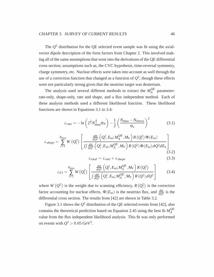
CHAPTER 3. SURVEY OF CURRENT RESULTS 46
TheQ2 distribution for the QE selected event sample was fit using the axial-
vector dipole description of the form factors from Chapter 2. This involved mak-
ing all of the same assumptions that went into the derivations of the QE differential
cross section; assumptions such as, the CVC hypothesis, time-reversal symmetry,
charge symmetry, etc. Nuclear effects were taken into account as well through the
use of a correction function that changed as a function ofQ2, though these effects
were not particularly strong given that the neutrino targetwas deuterium.
The analysis used several different methods to extract theMQEA parameter:
rate-only, shape-only, rate and shape, and a flux independent method. Each of
these analysis methods used a different likelihood function. These likelihood
functions are shown in Equations 3.1 to 3.4:
L rate = − ln
(
212N
12dataσN
)
− 12
(
Ndata−Ntheory
σn
)2
(3.1)
Lshape=Ndata
∑i=1
W(
Q2i
)
dσdQ2
(
Q2i ,Eνi ;M
QEA ,MV
)
R(
Q2i
)
Φ(Eνi)
RR dσdQ2
(
Q2i ,Eνi ;M
QEA ,MV
)
R(Q2)Φ(Eνi)dQ2dEν
(3.2)
L total = L rate+Lshape (3.3)
LFI =Ndata
∑i=1
W(
Q2i
)
dσdQ2
(
Q2i ,Eνi;M
QEA ,MV
)
R(
Q2i
)
R dσdQ2
(
Q2i ,Eνi;M
QEA ,MV
)
R(Q2)dQ2
(3.4)
whereW(
Q2)
is the weight due to scanning efficiency,R(
Q2i
)
is the correction
factor accounting for nuclear effects,Φ(Eνi) is the neutrino flux, anddσdQ2 is the
differential cross section. The results from [42] are shownin Table 3.2.
Figure 3.1 shows theQ2 distribution of the QE selected events from [42], also
contains the theoretical prediction based on Equation 2.45using the best fitMQEA
value from the flux independent likelihood analysis. This fitwas only performed
on events withQ2 > 0.05 GeV2.
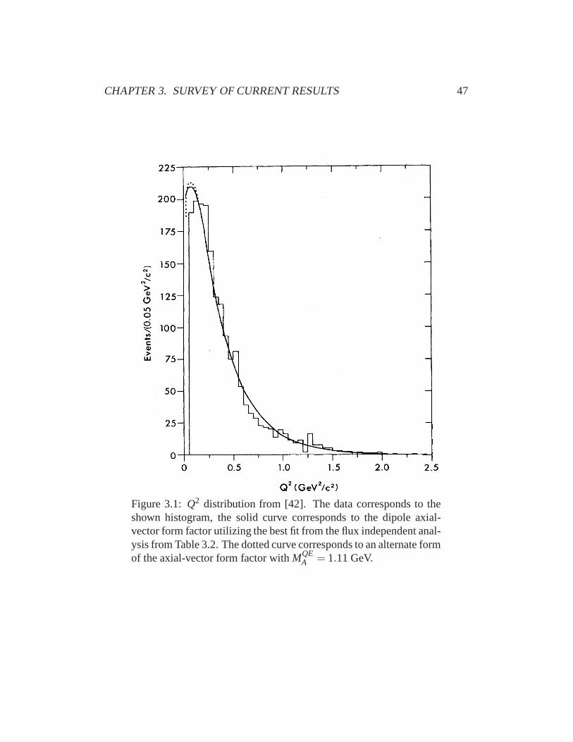
CHAPTER 3. SURVEY OF CURRENT RESULTS 47
Figure 3.1:Q2 distribution from [42]. The data corresponds to theshown histogram, the solid curve corresponds to the dipole axial-vector form factor utilizing the best fit from the flux independent anal-ysis from Table 3.2. The dotted curve corresponds to an alternate formof the axial-vector form factor withMQE
A = 1.11 GeV.
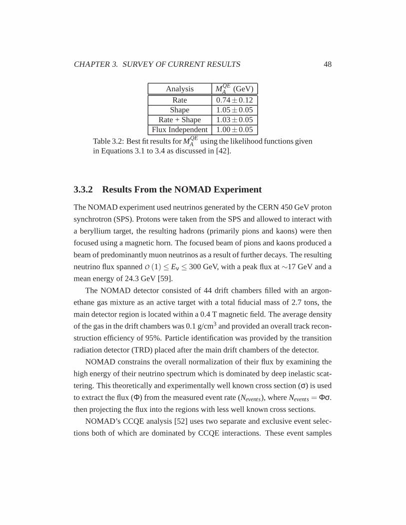
CHAPTER 3. SURVEY OF CURRENT RESULTS 48
Analysis MQEA (GeV)
Rate 0.74±0.12Shape 1.05±0.05
Rate + Shape 1.03±0.05Flux Independent 1.00±0.05
Table 3.2: Best fit results forMQEA using the likelihood functions given
in Equations 3.1 to 3.4 as discussed in [42].
3.3.2 Results From the NOMAD Experiment
The NOMAD experiment used neutrinos generated by the CERN 450 GeV proton
synchrotron (SPS). Protons were taken from the SPS and allowed to interact with
a beryllium target, the resulting hadrons (primarily pionsand kaons) were then
focused using a magnetic horn. The focused beam of pions and kaons produced a
beam of predominantly muon neutrinos as a result of further decays. The resulting
neutrino flux spannedO (1) ≤ Eν ≤ 300 GeV, with a peak flux at∼17 GeV and a
mean energy of 24.3 GeV [59].
The NOMAD detector consisted of 44 drift chambers filled withan argon-
ethane gas mixture as an active target with a total fiducial mass of 2.7 tons, the
main detector region is located within a 0.4 T magnetic field.The average density
of the gas in the drift chambers was 0.1 g/cm3 and provided an overall track recon-
struction efficiency of 95%. Particle identification was provided by the transition
radiation detector (TRD) placed after the main drift chambers of the detector.
NOMAD constrains the overall normalization of their flux by examining the
high energy of their neutrino spectrum which is dominated bydeep inelastic scat-
tering. This theoretically and experimentally well known cross section (σ) is used
to extract the flux (Φ) from the measured event rate (Nevents), whereNevents= Φσ.
then projecting the flux into the regions with less well knowncross sections.
NOMAD’s CCQE analysis [52] uses two separate and exclusive event selec-
tions both of which are dominated by CCQE interactions. These event samples
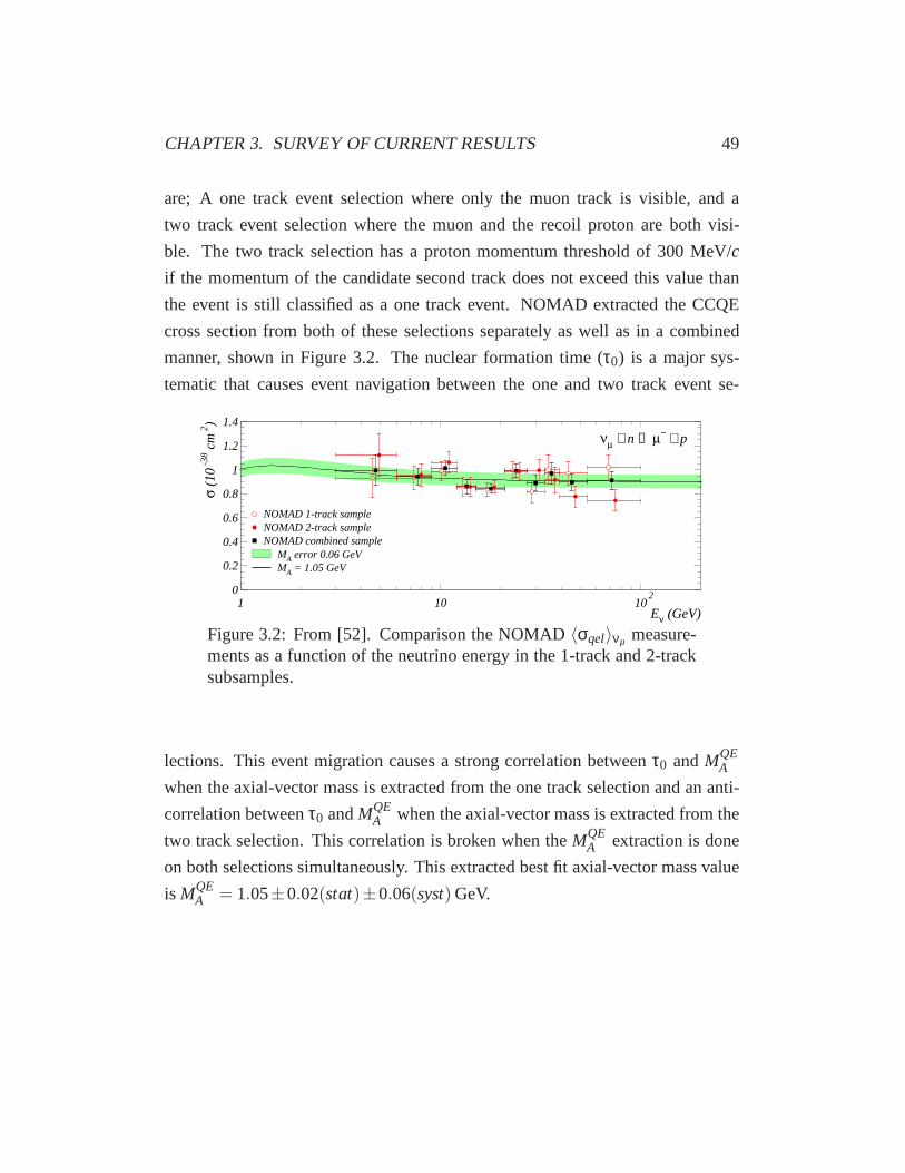
CHAPTER 3. SURVEY OF CURRENT RESULTS 49
are; A one track event selection where only the muon track is visible, and a
two track event selection where the muon and the recoil proton are both visi-
ble. The two track selection has a proton momentum thresholdof 300 MeV/c
if the momentum of the candidate second track does not exceedthis value than
the event is still classified as a one track event. NOMAD extracted the CCQE
cross section from both of these selections separately as well as in a combined
manner, shown in Figure 3.2. The nuclear formation time (τ0) is a major sys-
tematic that causes event navigation between the one and twotrack event se-
0
0.2
0.4
0.6
0.8
1
1.2
1.4
1 10 102
Eν (GeV)
σ (
10 -
38 c
m 2)
νµ + n → µ− + p
NOMAD 1-track sampleNOMAD 2-track sampleNOMAD combined sample
MA error 0.06 GeVMA = 1.05 GeV
Figure 3.2: From [52]. Comparison the NOMAD〈σqel〉νµ measure-ments as a function of the neutrino energy in the 1-track and 2-tracksubsamples.
lections. This event migration causes a strong correlationbetweenτ0 andMQEA
when the axial-vector mass is extracted from the one track selection and an anti-
correlation betweenτ0 andMQEA when the axial-vector mass is extracted from the
two track selection. This correlation is broken when theMQEA extraction is done
on both selections simultaneously. This extracted best fit axial-vector mass value
is MQEA = 1.05±0.02(stat)±0.06(syst) GeV.
CHAPTER 3. SURVEY OF CURRENT RESULTS 50
3.3.3 Results From the MiniBooNE Experiment
The MiniBooNE experiment has published two separate paperson CCQE scatter-
ing results: [31], and [34]. These publications documentedtwo separate analyses
that extracted different (though consistent) values of thetheMQEA parameter. The
first publication [31] presented a simple shape-only fit using the MiniBooNE MC
that attempted to parameterize the lowQ2 region by fitting for a Pauli blocking
parameter simultaneously. The second publication [34] produced a axial-vector
mass measurement as a side product to a more inclusive model independent cross-
section and double differential cross section measurementof the detector observ-
ables.
The MiniBooNE experiment at Fermi National Accelerator Lab(FNAL) mea-
sures a beam of muon neutrinos incident on 818 tons of mineraloil (CH5) con-
tained within a spherical detector of radius of 6.1 meters and surrounded by 1280
8in photo multiplier tubes (PMTs) which capture the Cherenkov light as charged
particles pass through the detector. The FNAL booster provides protons acceler-
ated to 8 GeV kinetic energy. The protons from the booster beam scatter off of a
beryllium target located inside a magnetic horn. The magnetic field provided by
the horn focuses primarilyπ+ but also focuses someK+. These hadrons will then
decay to anti-muons and muon neutrinos. Most of the anti-muons are absorbed
by the earth between the booster beam and the MiniBooNE detector leaving just
a beam of muon neutrinos. The booster generates a neutrino beam with a mean
neutrino energy of 0.7 GeV and has an energy distribution such that 99% of the
neutrinos have energy less than 2.5 GeV.
MiniBooNE identifies QE interaction candidates by looking for a lone muon
with no secondary hadron. MiniBooNE identifies muons by looking for the muon
ring and the secondary Michel electron ring from the decay ofthe muon. Looking
for the Michel electron helps to distinguish the muon ring from a potential pion
ring from an NC interaction where there will be two decay electrons from the pion
decay chain. This selection consisted of 193709 selected events, the estimated
efficiency was 35% with an estimated purity of 74%.
CHAPTER 3. SURVEY OF CURRENT RESULTS 51
The MiniBooNE Axial-Vector Mass Measurement
The MiniBooNE extraction of the axial-vector mass proceedsin a manner that is
similar to the way the ANL bubble chamber experiment measured MQEA , by fitting
theQ2 distribution of CC-νµ QE interactions for the axial-vector mass parameter
of the dipole form factor. The MiniBooNE experiment uses a Relativistic Fermi
Gas (RFG) model within their neutrino interaction simulation to model the scat-
tering of neutrinos off of carbon nuclei. It was necessary tofully understand any
sources of differences in the spectrum due to the interaction model for the pur-
poses of the MiniBooNE oscillation analysis [60], thus MiniBooNE attempted to
parameterize the lowQ2 region of theirQ2 spectrum where nuclear effects are ex-
pected to dominate. MiniBooNE did this by introducing an additional parameter,
κ, that changes the amount of Pauli-blocking in a QE interaction. MiniBooNE fits
the shape of theQ2 distribution all the down toQ2 = 0GeV2, from this fit Mini-
BooNE obtains the best fit values of:MQEA = 1.23±0.20GeV for the axial-vector
mass, andκ = 1.019±0.011. Figure 3.3 from [31] shows the data and best fit MC
Q2 distribution, along with a 1σ contour ofMQEA vs. κ.
The MiniBooNE QE Cross Section Measurement
Later MiniBooNE attempted a more sophisticated model independent measure-
ment of the CC-νµ QE double differential cross section with respect to the detec-
tor observables: muon kinetic energy (Tµ), and the muon scattering angle (θµ).
Because this analysis measured a cross section it was necessary to perform sev-
eral additional analysis steps that were not done in the MiniBooNE axial-vector
mass measurement. These additional steps included a correction to the distri-
bution based on the efficiency as a function of observables (Tµ and θµ), and a
subtraction of the non-CCQE background.
MiniBooNE does anin situ measurement of the non-CCQE background. The
in situ measurement is done by identifying an event sample that is dominated by
non-CCQE interactions. The MiniBooNE non-CCQE event selection looks for

CHAPTER 3. SURVEY OF CURRENT RESULTS 52
)2 (GeV2Q0 0.1 0.2 0.3 0.4 0.5 0.6 0.7 0.8 0.9 1
Eve
nts
0
2000
4000
6000
8000
10000
12000
14000
1 1.01 1.02 1.03 1.04 1.05
1.1
1.2
1.3
1.4
1.5
κ
(G
eV)
AM
Figure 3.3: From [31]. ReconstructedQ2 for νµ CCQE events in-cluding systematic errors. The simulation, before (dashed) and af-ter (solid) the fit, is normalized to data. The dotted (dot-dash) curveshows backgrounds that are not CCQE (not “CCQE-like”). The insetshows the 1σ CL contour for the best-fit parameters (star), along withthe starting values (circle), and fit results after varying the backgroundshape (triangle).
an additional (third) Cherenkov ring outside of the first twoCherenkov rings of
the CCQE selection. This non-CCQE event selection is composed of 90% events
with a single muon plus single pion in the final state. Muon plus single pion
are the dominant background to the CCQE selected events. TheCC1πMC event
sample is then reweighted such that the MC reconstructedQ2 distribution matches
the data reconstructedQ2 distribution. The MC CC1πcorrection function is then
applied to the MC CC1π background to the CCQE MC event sample, then an
equal number of events are subtracted from the CCQE data event sample. This

CHAPTER 3. SURVEY OF CURRENT RESULTS 53
0 0.1 0.2 0.3 0.4 0.5 0.6 0.7 0.8 0.9 1
Eve
nts
01000200030004000500060007000
(a) 2 subevent
)2 (GeVQE2Q
dataMC totalCCQE
+πCC1others
0 0.1 0.2 0.3 0.4 0.5 0.6 0.7 0.8 0.9 1
Eve
nts
0
500
1000
1500
2000
2500
(b) 3 subevent
)2 (GeVQE2Q
00.20.40.60.811.21.41.61.82
weight
+π
CC
1
Figure 3.4: From [34]. Distribution of events inQ2 QE for the (a) 2and (b) 3 subevent samples before the application of the CC1 back-ground correction. Data and MC samples are shown along with theindividual MC contributions from CCQE, CC1π, and other channels.In (b), the dashed line shows the CC1π reweighting function (withthe y-axis scale on the right) as determined from the background tprocedure.
gives an approximately pure sample of CCQE events. The CCQE and CC1πevent
samples are shown in Figure 3.4.
MiniBooNE uses the background subtracted (and efficiency corrected) CCQE
event sample to make measurements of the cross section as function of several
different kinematic variables. They also, as a separate measurement, perform a
fit of the Q2 distribution using the background subtracted data and MC, CCQE
selected events for the axial-vector mass and theκ parameter. This fit produces
best fit values ofMQEA = 1.35± 0.17 GeV andκ = 1.007± 0.012. This axial-
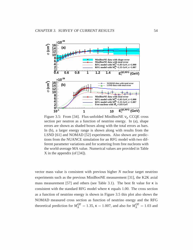
CHAPTER 3. SURVEY OF CURRENT RESULTS 54
0.4 0.6 0.8 1 1.2 1.4 1.6 1.8 2
)2 (
cmσ
02468
10121416
-3910×
MiniBooNE data with shape errorMiniBooNE data with total error
=1.000κ=1.03 GeV, effARFG model with M
=1.007κ=1.35 GeV, effARFG model with M
(GeV)QE,RFGνE
(a)
(GeV)QE,RFGνE-110 1 10
)2 (
cmσ
02468
10121416
-3910×
MiniBooNE data with total error=1.000κ=1.03 GeV, eff
ARFG model with M=1.007κ=1.35 GeV, eff
ARFG model with M=1.03 GeVAFree nucleon with M
NOMAD data with total errorLSND data with total error(b)
Figure 3.5: From [34]. Flux-unfolded MiniBooNEνµ CCQE crosssection per neutron as a function of neutrino energy. In (a),shapeerrors are shown as shaded boxes along with the total errors as bars.In (b), a larger energy range is shown along with results fromtheLSND [61] and NOMAD [52] experiments. Also shown are predic-tions from the NUANCE simulation for an RFG model with two dif-ferent parameter variations and for scattering from free nucleons withthe world-average MA value. Numerical values are provided in TableX in the appendix (of [34]).
vector mass value is consistent with previous higherN nuclear target neutrino
experiments such as the previous MiniBooNE measurement [31], the K2K axial
mass measurement [57] and others (see Table 3.1). The best fitvalue for κ is
consistent with the standard RFG model whereκ equals 1.00. The cross section
as a function of neutrino energy is shown in Figure 3.5 this plot also shows the
NOMAD measured cross section as function of neutrino energyand the RFG
theoretical prediction forMQEA = 1.35, κ = 1.007, and also forMQE
A = 1.03 and
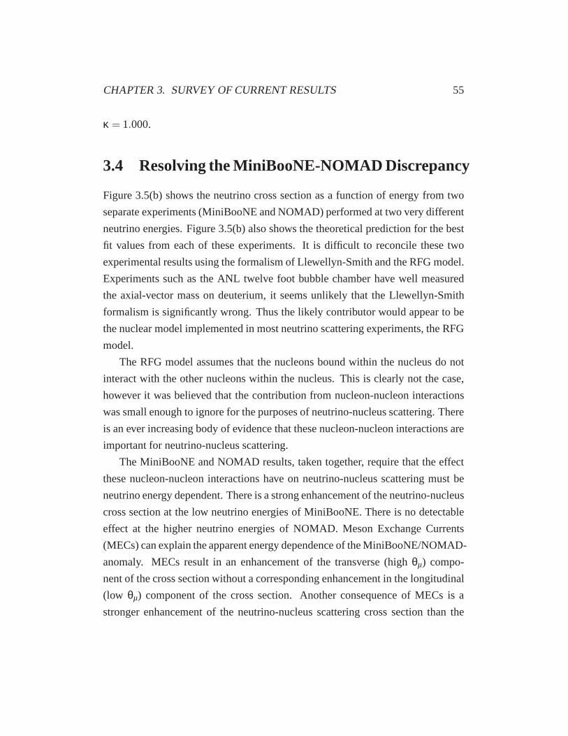
CHAPTER 3. SURVEY OF CURRENT RESULTS 55
κ = 1.000.
3.4 Resolving the MiniBooNE-NOMAD Discrepancy
Figure 3.5(b) shows the neutrino cross section as a functionof energy from two
separate experiments (MiniBooNE and NOMAD) performed at two very different
neutrino energies. Figure 3.5(b) also shows the theoretical prediction for the best
fit values from each of these experiments. It is difficult to reconcile these two
experimental results using the formalism of Llewellyn-Smith and the RFG model.
Experiments such as the ANL twelve foot bubble chamber have well measured
the axial-vector mass on deuterium, it seems unlikely that the Llewellyn-Smith
formalism is significantly wrong. Thus the likely contributor would appear to be
the nuclear model implemented in most neutrino scattering experiments, the RFG
model.
The RFG model assumes that the nucleons bound within the nucleus do not
interact with the other nucleons within the nucleus. This isclearly not the case,
however it was believed that the contribution from nucleon-nucleon interactions
was small enough to ignore for the purposes of neutrino-nucleus scattering. There
is an ever increasing body of evidence that these nucleon-nucleon interactions are
important for neutrino-nucleus scattering.
The MiniBooNE and NOMAD results, taken together, require that the effect
these nucleon-nucleon interactions have on neutrino-nucleus scattering must be
neutrino energy dependent. There is a strong enhancement ofthe neutrino-nucleus
cross section at the low neutrino energies of MiniBooNE. There is no detectable
effect at the higher neutrino energies of NOMAD. Meson Exchange Currents
(MECs) can explain the apparent energy dependence of the MiniBooNE/NOMAD-
anomaly. MECs result in an enhancement of the transverse (high θµ) compo-
nent of the cross section without a corresponding enhancement in the longitudinal
(low θµ) component of the cross section. Another consequence of MECs is a
stronger enhancement of the neutrino-nucleus scattering cross section than the

CHAPTER 3. SURVEY OF CURRENT RESULTS 56
Figure 3.6: From [62]. Left: The QE differential cross section(dσ/dQ2) as a function ofQ2 for νµ, νµ energies of 1.0 GeV (max-imum accessibleQ2
max = 1.3 (GeV/c)2). Here, the orange dot-ted line is the prediction of the ”Independent Nucleon (MA=1.014)”model. The blue dashed line is the prediction of the the ”LargerMA (MA=1.3)” model. The red line is prediction of the ”Trans-verse Enhancement” model. Top (a):νµ differential QE cross sec-tions. Bottom (b): νµ differential QE cross sections. Right: Sameas Left forνµ, νµ energies of 3.0 GeV (maximum accessibleQ2
max=4.9 (GeV/c)2).

CHAPTER 3. SURVEY OF CURRENT RESULTS 57
antineutrino-nucleus scattering cross section. As shown in Figure 3.6 from [62]
the transversely enhanced neutrino-carbon differential cross section of 1 GeV neu-
trinos is∼25% larger than the neutrino-nulceon differential cross section of 1 GeV
neutrinos. While the transversely enhanced antineutrino-carbon cross section is
∼5% larger than the neutrino-nucleon cross section. This trend is smaller for the
3 GeV neutrinos/antineutrinos.
The other possibility is that this is not a neutrino energy effect but is instead
because of final state identification. The MiniBooNE QE identification procedure
does not use any information about the presence of the recoilproton in the final
state, because the MiniBooNE detector is very insensitive to the presence of the
recoil proton. This is contrasted with the NOMAD experimentwhich is very
good at identifying the presence of final state particles. NOMAD has a proton
momentum threshold of 300 MeV/c; above this threshold the event is classified
as a candidate two track event, below this threshold the event is classified as a
one track event. It is possible that this discrepancy in finalstate identification is
responsible for the discrepancy in the measured axial-vector mass values. This
would happen if NOMAD rejected as being not QE like interactions that have
additional particles in the final state that would appear as aresult of the nucleon-
nucleon interactions, while MiniBooNE would not be able to distinguish these
interactions from QE interactions.

Chapter 4
MINOS Experiment
The Main Injector Neutrino Oscillation Search (MINOS) experiment [63] uses
two nearly identical neutrino detectors positioned 734 km away from each other.
The two detectors measure the energy spectrum of the neutrino beam produced by
the Neutrinos at the Main Injector (NuMI) facility at FNAL [64] with a baseline
of 734 km. The neutrinos pass through the Near Detector (ND) approximately
1 km from the NuMI production target. The neutrinos then passthrough 734 km
of earth before reaching the Far Detector (FD) at the end of the baseline. The
general geographic layout of the MINOS experiment is shown in Figure 4.1. For
more details about the MINOS experimental configuration see[65].
4.1 The NuMI Beamline
The first stage of proton acceleration is the FNAL linear accelerator (Linac) which
accelerates the protons up to 400 MeV/c. The Booster circular accelerator takes
protons from the linac and accelerates them up to 8 GeV/c. TheBooster then feeds
the protons into the Main Injector (MI) circular accelerator which accelerates the
protons up to 120 GeV/c which finally feeds into the Tevatron.While accelerating
the protons up to 120 GeV/c the MI forms the protons into sevenbatches in the
MI. Of these seven, two would go to the Tevatron while the restwould be used
58
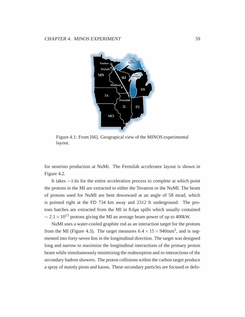
CHAPTER 4. MINOS EXPERIMENT 59
Figure 4.1: From [66]. Geograpical view of the MINOS experimentallayout.
for neutrino production at NuMi. The Fermilab accelerator layout is shown in
Figure 4.2.
It takes∼1.6s for the entire acceleration process to complete at which point
the protons in the MI are extracted to either the Tevatron or the NuMI. The beam
of protons used for NuMI are bent downward at an angle of 58 mrad, which
is pointed right at the FD 734 km away and 2312 ft underground.The pro-
tons batches are extracted from the MI in 8.6µs spills which usually contained
∼ 2.1×10¹³ protons giving the MI an average beam power of up to 400kW.
NuMI uses a water-cooled graphite rod as an interaction target for the protons
from the MI (Figure 4.3). The target measures 6.4×15×940mm3, and is seg-
mented into forty-seven fins in the longitudinal direction.The target was designed
long and narrow to maximize the longitudinal interactions of the primary proton
beam while simultaneously minimizing the reabsorption andre-interactions of the
secondary hadron showers. The proton collisions within thecarbon target produce
a spray of mainly pions and kaons. These secondary particlesare focused or defo-
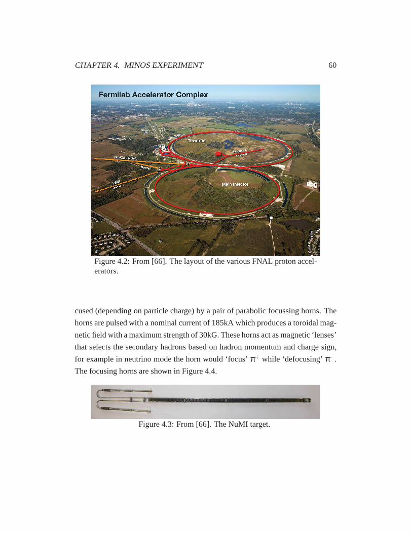
CHAPTER 4. MINOS EXPERIMENT 60
Figure 4.2: From [66]. The layout of the various FNAL proton accel-erators.
cused (depending on particle charge) by a pair of parabolic focussing horns. The
horns are pulsed with a nominal current of 185kA which produces a toroidal mag-
netic field with a maximum strength of 30kG. These horns act asmagnetic ‘lenses’
that selects the secondary hadrons based on hadron momentumand charge sign,
for example in neutrino mode the horn would ‘focus’π+ while ‘defocusing’π−.
The focusing horns are shown in Figure 4.4.
Figure 4.3: From [66]. The NuMI target.

CHAPTER 4. MINOS EXPERIMENT 61
Once the charged hadrons have been focused (or defocused) bythe magnetic
horns, the focused particles enter a 675m long, evacuated (and later helium filled)
decay pipe. Here many of the secondary hadrons (mostly pionsand kaon) decay
to neutrinos via a process similar toπ→ µ+ + νµ. Hadrons that do not decay
within the decay pipe are stopped by a 5m hadron absorber which consists of a
water cooled aluminum core surrounded by steel blocks and a layer of concrete.
Figure 4.4: From [66]. Left: Photograph of inner conductorsof theNuMI parabolic focusing horn. Right: Photograph of the firstfocus-ing horn.
After the undecayed hadrons have been stopped by the hadron absorber, the
tertiary beam of muons are stopped by the 300m of dolomite rock that lies be-
tween the NuMI target and the MINOS ND cavern. This leaves a beam of the
neutrinos whose path will take them through the MINOS ND and later the MI-
NOS FD. A schematic of the various components of the NuMI beamline is shown

CHAPTER 4. MINOS EXPERIMENT 62
in Figure 4.5. The NuMI beam is composed of∼97.8%νµ with the majority of
the contamination coming from∼1.8% νµ and the remaining∼0.4%νe. These
estimates come from a MC simulation of the neutrino beamlineand hadron pro-
duction off of the NuMI target.
Figure 4.5: From [66]. The various components of the NuMI beam-line.
NuMI was designed to be capable of many different experimental modes.
The neutrino energy spectrum can be tuned by changing eitherthe current going
through the focusing horns or changing the position of the target relative to the
first focusing horn. These changes result in the focusing of different momentum
hadrons, which in turn leads to different energies of the tertiary neutrino beam.
The direction can also be reversed which changes the charge sign of the particles
focused and defocused which will produce a beam composed of predominantly
νµ.
4.2 The MINOS Detectors
Throughout the development of the MINOS experiment three distinct detectors
have been used: the Near and Far detectors which measure the energy spectrum
of the NuMI neutrino beam, and the smaller Calibration detector (CalDet) which
was exposed to a test beam at the CERN proton synchrotron. Theresults from
CalDet are used to characterize the response of the other MINOS detectors to
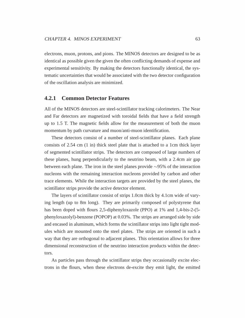
CHAPTER 4. MINOS EXPERIMENT 63
electrons, muon, protons, and pions. The MINOS detectors are designed to be as
identical as possible given the given the often conflicting demands of expense and
experimental sensitivity. By making the detectors functionally identical, the sys-
tematic uncertainties that would be associated with the twodetector configuration
of the oscillation analysis are minimized.
4.2.1 Common Detector Features
All of the MINOS detectors are steel-scintillator trackingcalorimeters. The Near
and Far detectors are magnetized with toroidal fields that have a field strength
up to 1.5 T. The magnetic fields allow for the measurement of both the muon
momentum by path curvature and muon/anti-muon identification.
These detectors consist of a number of steel-scintillator planes. Each plane
consists of 2.54 cm (1 in) thick steel plate that is attached to a 1cm thick layer
of segmented scintillator strips. The detectors are composed of large numbers of
these planes, hung perpendicularly to the neutrino beam, with a 2.4cm air gap
between each plane. The iron in the steel planes provide∼95% of the interaction
nucleons with the remaining interaction nucleons providedby carbon and other
trace elements. While the interaction targets are providedby the steel planes, the
scintillator strips provide the active detector element.
The layers of scintillator consist of strips 1.0cm thick by 4.1cm wide of vary-
ing length (up to 8m long). They are primarily composed of polystyrene that
has been doped with flours 2,5-diphenyloxazole (PPO) at 1% and 1,4-bis-2-(5-
phenyloxazolyl)-benzene (POPOP) at 0.03%. The strips are arranged side by side
and encased in aluminum, which forms the scintillator strips into light tight mod-
ules which are mounted onto the steel plates. The strips are oriented in such a
way that they are orthogonal to adjacent planes. This orientation allows for three
dimensional reconstruction of the neutrino interaction products within the detec-
tors.
As particles pass through the scintillator strips they occasionally excite elec-
trons in the flours, when these electrons de-excite they emitlight, the emitted
CHAPTER 4. MINOS EXPERIMENT 64
light is collected by 1.2mm diameter wavelength shifting (WLS) optical fibers.
The optical fibers are glued into a 2mm groove that runs along the center of the
scintillator strip. The WLS fiber change the average wavelength of the emitted
light from blue region (460nm) to the green region (530nm). The strips are coated
with a TiO2 doped paint, which helps to reflect and trap the scintillation light,
which maximizes the likelihood that the light will be collected by the WLS fibers.
The WLS fiber is routed from the individual strips and collected into a manifold
which guides the fibers into an optical connection. Figure 4.6 shows an individual
scintillator strip along with strips that have collected into strip module.
Figure 4.6: From [66]. Left: Individual scintillator strip. Right: Stripsthat have collected into a detector module.
Once photons reach the optical connector, they are routed via clear optical
fibers to multi anode photomultiplier tubes (PMTs). Clear optical fibers are used
because they have a much longer attenuation length. The PMTsare used to turn
the optical signal from the scintillator into an electronicsignal that can be pro-
cessed by the data acquisition (DAQ) system. A schematic of this system is shown
in Figure 4.7.

CHAPTER 4. MINOS EXPERIMENT 65
Figure 4.7: From [66]. Schematic of a scintillator plane readout sys-tem.
4.2.2 The Calibration Detector
The Calibration detector weighed 12 tons and was constructed to measure the
response and topology of the Near and Far detectors to hadronic and leptonic
particles passing through the detector elements. CalDet was active from 2001-
2003 and exposed to beams composed ofp+, e±, µ±, andπ± in the few-GeV

CHAPTER 4. MINOS EXPERIMENT 66
region at the CERN proton synchrotron accelerator. CalDet consisted of sixty 1 m
square planes, each plane is composed of twenty four scintillator strips. CalDet
was configured so that it could be operated with electronics and readouts that
either simulated the Near or Far detector systems. CalDet was also equipped with
a time-of-flight system, which acted as a trigger and discriminated betweene, π,
andp, and a Cherenkov counters that were used to tag electrons in the detector. A
photograph of the Calibration detector is shown in Figure 4.8.
Figure 4.8: From [66]. Photograph of the MINOS Calibration detec-tor.
4.2.3 The Far Detector
The MINOS Far detector, at 5.4 kT is the largest of the MINOS detectors. The Far
detector lies in the Soudan Underground Laboratory in Soudan Minnesota 2312 ft
(705 m) underground and 735 km away from the NuMI target. The Far detector is
composed of a total of 484 planes formed into an octagonal cylinder that measures
8 m across. Due to limitations on the length of the coil that supplies the magnetic
field the to Far detector, the Far detector is divided into two‘supermodules’, sep-
arated by an air gap of 1.2 m. The individual supermodules arecomposed of 249
planes and 237 planes, and each are independently magnetized. Each of the coils
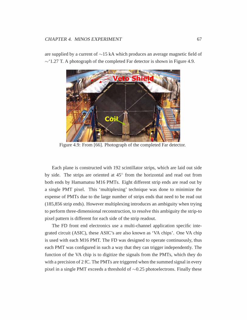
CHAPTER 4. MINOS EXPERIMENT 67
are supplied by a current of∼15 kA which produces an average magnetic field of
∼‘1.27 T. A photograph of the completed Far detector is shown in Figure 4.9.
Figure 4.9: From [66]. Photograph of the completed Far detector.
Each plane is constructed with 192 scintillator strips, which are laid out side
by side. The strips are oriented at 45◦ from the horizontal and read out from
both ends by Hamamatsu M16 PMTs. Eight different strip ends are read out by
a single PMT pixel. This ‘multiplexing’ technique was done to minimize the
expense of PMTs due to the large number of strips ends that need to be read out
(185,856 strip ends). However multiplexing introduces an ambiguity when trying
to perform three-dimensional reconstruction, to resolve this ambiguity the strip-to
pixel pattern is different for each side of the strip readout.
The FD front end electronics use a multi-channel application specific inte-
grated circuit (ASIC), these ASIC’s are also known as ‘VA chips’. One VA chip
is used with each M16 PMT. The FD was designed to operate continuously, thus
each PMT was configured in such a way that they can trigger independently. The
function of the VA chip is to digitize the signals from the PMTs, which they do
with a precision of 2 fC. The PMTs are triggered when the summed signal in every
pixel in a single PMT exceeds a threshold of∼0.25 photoelectrons. Finally these
CHAPTER 4. MINOS EXPERIMENT 68
front end electronic boards time stamp the signal with a precision of 1.56 ns.
The signal collected from the front end boards are pedestal suppressed, then
passed to a computer farm, the computer farm then applies higher level trigger-
ing conditions which help determine whether the data shouldbe saved. The pri-
mary triggering condition is the ‘spill trigger’, which determines whether the FD
readout is coincident with a beam spill from the MI. GPS clocks are used to the
synchronize the Near and Far detectors. When a beam spill occurs at the MI, a
time stamped signal is sent to the FD through an internet connection. The FD will
record all of the hit information in a time window 80µs wide and centered on the
time of the MI beam spill. This ‘spill window’ can be extendedto ensure that
there is an activity free period of at least 156 ns so that a candidate neutrino event
wont be split into two separate spill windows.
4.2.4 The Near Detector
The Near detector is the smaller of the two primary MINOS detectors with a mass
of ∼980 tons, it is located∼320ft (∼98 m) underground on site at FNAL∼1km
from the NuMI target. Because the neutrino beam has divergedvery little in the
∼1 km between the target and the ND, and NuMI has an inherently high neutrino
rate, the ND was designed to be able to contend with this high interaction rate.
The ND is composed of 282 planes arranged in a ‘squashed’ octagonal shape,
where each plane is 6.2 m wide and 3.8 m high. There is a 30× 30cm2 hole
offset 0.56 m from the horizontal center of the ND through which the coil that
supplies the magnetic field passes through. The center of theneutrino beam spot
lies 0.93 m from the horizontal center of the plane, in the opposite direction of the
coil. The magnetic field coil carries a current of 40kA which creates a magnetic
field of 1.17 T in the vicinity of the beam center. Figure 4.10 shows a photograph
of the Near detector.
The ND is divided into two different components: the first 120upstream
planes compose the calorimeter region, while the remainingdownstream planes
compose the spectrometer region. The calorimeter region isdesigned to maxi-
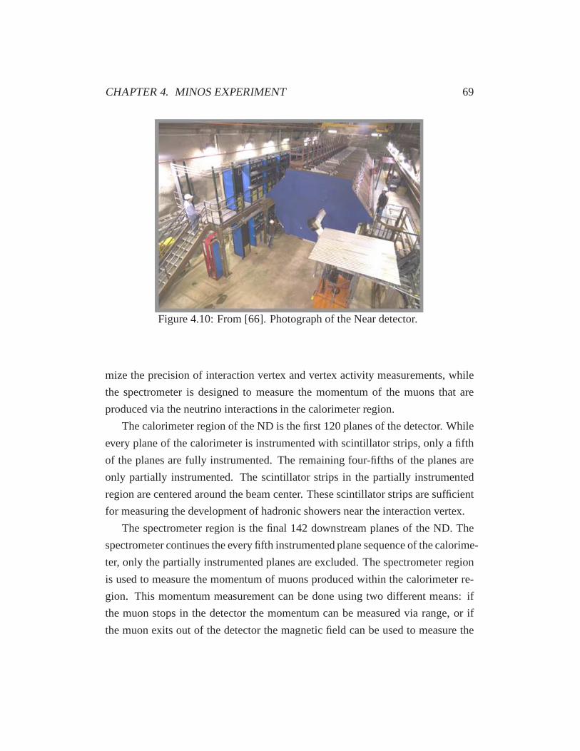
CHAPTER 4. MINOS EXPERIMENT 69
Figure 4.10: From [66]. Photograph of the Near detector.
mize the precision of interaction vertex and vertex activity measurements, while
the spectrometer is designed to measure the momentum of the muons that are
produced via the neutrino interactions in the calorimeter region.
The calorimeter region of the ND is the first 120 planes of the detector. While
every plane of the calorimeter is instrumented with scintillator strips, only a fifth
of the planes are fully instrumented. The remaining four-fifths of the planes are
only partially instrumented. The scintillator strips in the partially instrumented
region are centered around the beam center. These scintillator strips are sufficient
for measuring the development of hadronic showers near the interaction vertex.
The spectrometer region is the final 142 downstream planes ofthe ND. The
spectrometer continues the every fifth instrumented plane sequence of the calorime-
ter, only the partially instrumented planes are excluded. The spectrometer region
is used to measure the momentum of muons produced within the calorimeter re-
gion. This momentum measurement can be done using two different means: if
the muon stops in the detector the momentum can be measured via range, or if
the muon exits out of the detector the magnetic field can be used to measure the

CHAPTER 4. MINOS EXPERIMENT 70
momentum from curvature of the track. A schematic illustrating the differences
between a partially instrumented and a fully instrumented plane is shown in Fig-
ure 4.11.
Figure 4.11: From [65]. Strip configuration of the MINOS ND, di-vided into partially instrumented (above) and fully instrument (be-low)planes, and also U-view (left) and V-view (right) planes.
The ND strips are readout from only one end (unlike the FD). This is because
the scintillator strips for the ND are shorter than the scintillator strips used in the
FD. To compensate for the single read out end and also to maximize the light col-
lection, the end opposite from the read out end is coated witha reflective material.
These strips are read out using Hamamatsu M64 multi-anode PMTs, each partially
instrumented plane requires a single PMT for readout, whilea fully instrumented
planes requires one and a half PMTs for readout. The amount ofinstrumentation
is reduced in the spectrometer by summing the signal from sets of four pixels into
a single electronics channel. The adjacent pixels are not connected to adjacent
strips, thus the four-fold ambiguity can be resolved through the tracking of events

CHAPTER 4. MINOS EXPERIMENT 71
in the calorimeter (where there is no ambiguity) into the spectrometer allowing
for discrimination between the four possibilities. Thus itis not possible to resolve
this ambiguity for events whose vertex doesn’t lie within the calorimeter.
On average there are sixteen neutrino interactions in the NDduring each beam
spill (when in the L010z185i beam configuration). Thus the NDrequires special
high speed and deadtime less front end electronics. This electronic system is
based on the QIE chips that were used in the CDF and KTEV experiments and
developed at FNAL. The primary trigger is the spill trigger,when triggered for a
13 µs window the output of every PMT pixel is readout starting 1.5µs before the
beamspill.
Chapter 5
MINOS Data and Monte Carlo
5.1 MINOS Data
This analysis will use data collected using just the Near detector. The data was
collected during the first MINOS data taking run, from May 20,2005 through
February 2, 2006. This constituted∼1.27×1026 protons on target (POT) at NuMI.
The data as originally recorded by the MINOS ND consists of PMT pixel pulse
height as a function of time with nanosecond precision. Thisinformation about
single detector strips needs to be calibrated for the individual strip along with
a calibration for the location along the strip. Then the reconstruction software
associates the information about individual hits into higher level reconstructed
quantities such as tracks and showers, which are grouped into events (tracks and
showers that are associated by space and time in the detector) ideally these events
represent a single neutrino interaction within the detector.
5.1.1 Reconstruction
The MINOS reconstruction software uses the raw data of the energy deposited
within a strip and the strip location within the detector to attempt to identify the
path of individual higher energy particles (tracks) or cascades of lower energy par-
72
CHAPTER 5. MINOS DATA AND MONTE CARLO 73
ticles (showers). In the ND there are up to sixteen neutrino interactions per beam
spill. Every neutrino interaction will produce several secondary particles. Thus
there will be as few as 20 and possibly many more potentially visible particles
produced in the ND in a single beam spill. The first reconstruction step in the ND
is to group together hits that are near each other (both spatially and temporarily).
These slices of the beam spill trigger are assumed to be due toa single neutrino
interaction.
Tracks
When a massive charged particle relativistically passes through matter, the parti-
cle looses energy through the ionization of the surroundingmaterial and through
the excitation of nearby nuclei. The rate of energy loss is given by [67], which
contains updated tables of muon energy loss in matter. Included in [67] are up-
dates to the Bethe-Bloch theory of ionization energy loss [68]. The Bethe-Bloch
equation describes the energy loss (due to ionization) of particles as they pass
through matter, the full Bethe-Bloch equation is:
−dEdx
= Kz2ZA
1β2
[
12
ln
(
2mec2β2γ2Tmax
I2
)
−β2− δ(βγ)2
]
(5.1)
where
Tmax=2mec2β2γ2
1+2γme/M +(me/M)2 (5.2)
is the maximum kinetic energy that can be transferred to a free electron in a single
collision. z is the charge of the incident particle relative to the electrons charge,
I is the average excitation energy of the medium,Z is the atomic mass andA
is the atomic number or the medium.me is the mass of the electron,M is the
mass of the incident particle.K is an amalgamation of several constants:K/A =
4πNAr2emec2 ≈ 0.307 MeVg−1cm2 for A = 1, wherere is the charge radius of the
electron andNA is Avogadro’s number.
In Equation 5.1, theδ(βγ) term is a correction that accounts for ionization

CHAPTER 5. MINOS DATA AND MONTE CARLO 74
energy lossed due to the effect of the medium density, this term can be neglected
for βγ≈ 100. There are other possible radiative processes when charged particles
pass through matter, such asbremsstrahlungande+e− pair production, however
these effects can be neglected for muons with energy less than∼ 400 GeV [68].
The minimum of the Bethe-Bloch equation (Equation 5.1) as a function ofβγoccurs between 2< βγ< 4, while the Bethe-Bloch equation plateaus at higher en-
ergies, wheredEdx is slightly larger thandE
dx
∣
∣
min. Particles withβγnear the minimum
energy loss are called Minimum Ionizing Particles (MIP). Muons produced in the
ND from CC interactions are usually relativistic, and thus are minimum-ionizing.
After a particle has lost enough energy to no longer be minimum-ionizing the par-
ticle will lose increasingly more energy per distance traveled. The stopping power
of muons as a function of muon momentum for both data and MC along with the
Bethe-Bloch equation is shown in Figure 5.1.
Muons in the ND are produced with energy& 1 GeV, and are thus relativis-
tic and minimum-ionizing. The kinetic energy of the muons produced within the
ND can be estimated to first order by simply counting the number of planes that
the muon passes through before the muon stops. This approximation improves
as the muon gets closer to normal incidence, where the approximation becomes
exact. This is unlikely to happen because the muon will usually carry some trans-
verse momentum from the neutrino CC interaction, and the curvature due to the
magnetic field. MINOS has good energy resolution fromdEdx in the steel planes,
with σstopEµ
= 2%. The uncertainty in the energy of the stopping muon track is due
to the uncertainty in the total path length of the muon and theuncertainty in the
thickness of the individual planes.
While it is possible to measure the muon energy from the muon’s track length,
this requires that muon stop within the ND, it is also possible that the muon exits
the instrumented region of the detector before stopping. This makes an estimate
of the muon energy from the Bethe-Bloch equation impossible. When a muon
exits the the instrumented region of the ND before stopping it is still possible to
estimate the muon momentum from the curvature of the track. Estimating the

CHAPTER 5. MINOS DATA AND MONTE CARLO 75
Muon momentum (GeV/c)0 0.2 0.4 0.6 0.8 1 1.2 1.4 1.6 1.8 2
/g)
2S
topp
ing
pow
er (
MeV
cm
1.9
1.95
2
2.05
2.1
2.15
2.2
2.25
2.3
Bethe-Bloch
Monte Carlo
Data
Figure 5.1: From [65]. Stopping power for muons. The gray lineshows the Bethe-Bloch calculation of the stopping power formuonsin polystyrene scintillator. The solid circles and open triangles showthe response of stopping muons in the far detector data and GEANT3Monte Carlo simulations respectively. Both data and Monte Carlopoints have been normalized to the Bethe-Bloch calculationto givethe expected stopping power at the minimum ionizing point.
muon momentum from track curvature is done through the use ofa Kalman filter
algorithm [69][70].
The Kalman filter algorithm is a iterative algorithm for calculating the path
of an object based on sparse (and potentially incomplete) data. The advantage of
using the Kalman filter is that the filter can apply known physics to assist the al-
gorithm as the algorithm attempts to make predictions. The Kalman filter predicts
the value of five different parameters that describe the muons path through the
detector medium and the applied magnetic field, these parameters areu, v, dudz,
dvdz,
andq/p, whereu, v are the transverse position of the strips in the detector coordi-
nate system,z is the longitudinal position of the strips,q is the charge expressed
relative to the electron’s charge, andp is the momentum of the muon. The first
four variables are known from point to point and serve as input at each iteration

CHAPTER 5. MINOS DATA AND MONTE CARLO 76
step, while the last variable (q/p) is the final output of the Kalman filter. The
muon is tracked by the Kalman filter through the entire lengthof the track, it takes
both energy loss due to ionization and the bending of the muon’s path due to the
magnetic field into account when making predictions for the next iteration.
Another output of the Kalman filter is an error matrix that expresses the ac-
curacy of the filter’s predictions at each iteration step. Information from the error
matrix can be used to calculate an estimate of the uncertainty in the quantityq/p,
σq/p. Multiple scattering of the muon is the most important contribution to the
estimation ofσq/p. Multiple scattering is the scattering of the muon off of many
different nuclei, which causes small perturbations in the muon’s position (and
their derivatives) within an individual strip. These smallperturbations cause the
measurement of the muon’s momentum from curvature to be lessprecise than the
momentum from range, the uncertainty in the muon momentum from curvature is
5%.
Showers
No attempt is made by the standard MINOS reconstruction to reconstruct individ-
ual particles produced as a result of neutrino induced hadronic showers. Instead,
calorimetric information about the showers are used to estimate the total energy
of the shower.
When a neutrino interacts with a nucleus, the neutrino will transfer some frac-
tion of it’s initial momentum to the scattering target. Often this transferred mo-
mentum is enough to produce a shower large enough to be visible in the detector.
Because the secondary particles produced during a hadronicshower are hadrons,
the secondary particles will lose energy by interacting viathe strong force, this
will produce more low-energy hadrons, and though many of theparticles pro-
duced during a hadron shower will also lose energy through the Bethe-Bloch pro-
cess, the dominant processes is through strong interactions. As hadronic showers
develop many different strong processes along with nuclearprocesses effect the
development of the shower. Some of these processes such as pion absorption and

CHAPTER 5. MINOS DATA AND MONTE CARLO 77
neutron production are very difficult to see within the MINOSdetectors. These
effects cause the resolution on the shower energy to be large(relative to the muon
track energy). This energy resolution along with the absolute energy measurement
is very dependent on the energy calibration of the detectors, which is discussed in
the next section (Section 5.1.2).
5.1.2 Calibration
Calibration of the MINOS detectors is done by combining information from the
CalDet detector, cosmic-ray muons, test-bench measurements of the scintillator
systems, and a LED-based light-injection (LI) system. The purpose of the cali-
bration procedure is to receive as input the raw detector outputQraw(d,s, t,x) and
convert it into a fully corrected signalQcor whered is the detector used,s is the
strip the signal comes from,t the time the signal was recorded, andx is the po-
sition along the strip from which the signal originated. This correction is done
through the use of calibration-constants which are scale factors on the raw signal
Qraw:
Qcor = Qraw×D(d, t)×L(d,s,Qraw)×S(d,s)×A(d,s,x)×M (d) (5.3)
the constantsD, L, S, A, M correspond to the following corrections:
• Drift Correction ( D): a correction that removes the changes to the detector
response as function of time. Detector components, such as PMTs, detector
electronics, and the scintillator can change their response simply due to the
passage of time. This correction is an attempt to account forthose changes.
This correction was originally performed use the LI data, tomeasure the
individual changes of the strips, however it was discoveredthat the time
drift of the individual strips was consistent enough for thedrift calibration
to be performed from the mean signal per plane that comes fromcosmic
ray muons that completely pass through the detector. Any remaining differ-
ences between strip outputs can be corrected away by the strip-to-strip cor-
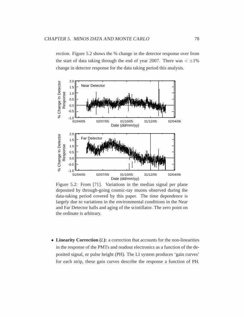
CHAPTER 5. MINOS DATA AND MONTE CARLO 78
rection. Figure 5.2 shows the % change in the detector response over from
the start of data taking through the end of year 2007. There was < ±1%
change in detector response for the data taking period this analysis.
Date (dd/mm/yy)01/04/05 02/07/05 01/10/05 31/12/05 02/04/06
Res
pons
e %
Cha
nge
In D
etec
tor
-1.0
-0.5
0.0
0.5
1.0
1.5
2.0Near Detector
Date (dd/mm/yy)01/04/05 02/07/05 01/10/05 31/12/05 02/04/06
Res
pons
e %
Cha
nge
In D
etec
tor
-1.0
-0.5
0.0
0.5
1.0
1.5
2.0Far Detector
Figure 5.2: From [71]. Variations in the median signal per planedeposited by through-going cosmic-ray muons observed during thedata-taking period covered by this paper. The time dependence islargely due to variations in the environmental conditions in the Nearand Far Detector halls and aging of the scintillator. The zero point onthe ordinate is arbitrary.
• Linearity Correction ( L): a correction that accounts for the non-linearities
in the response of the PMTs and readout electronics as a function of the de-
posited signal, or pulse height (PH). The LI system produces‘gain curves’
for each strip, these gain curves describe the response a function of PH.
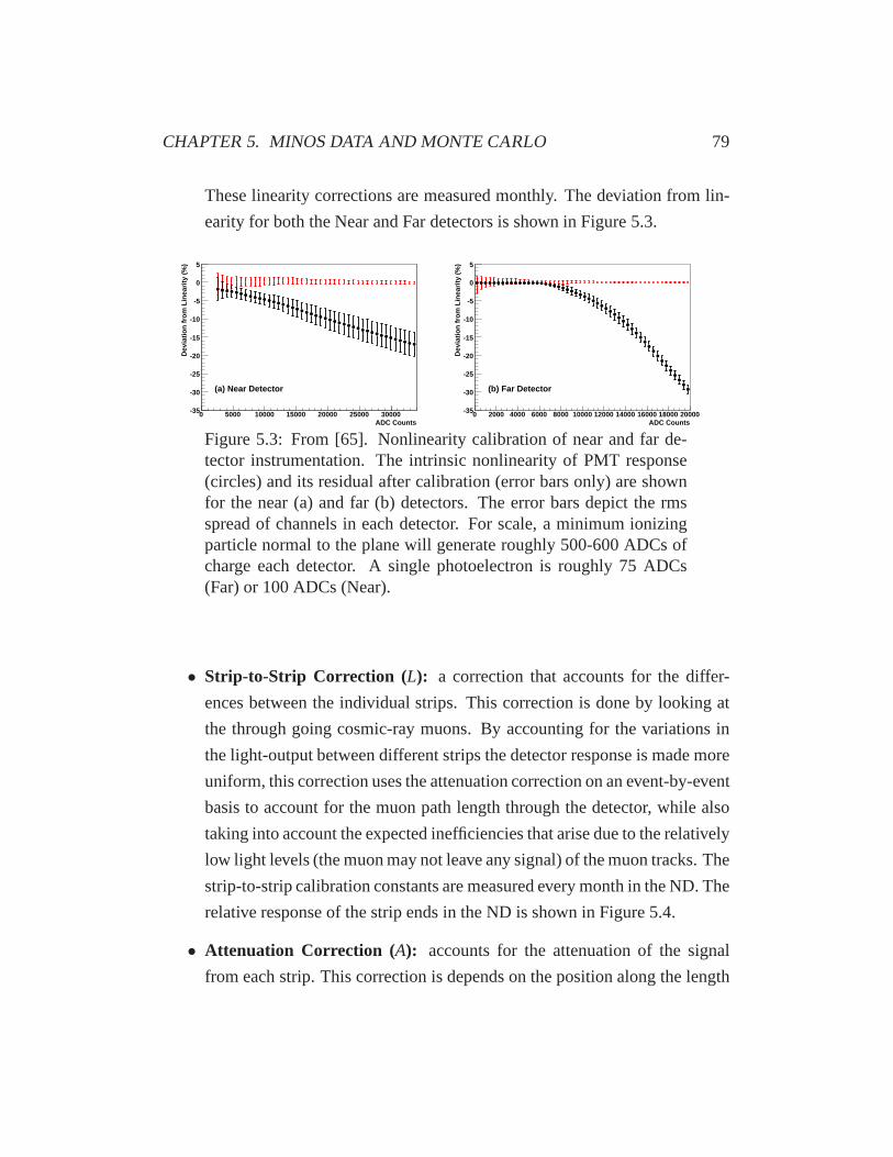
CHAPTER 5. MINOS DATA AND MONTE CARLO 79
These linearity corrections are measured monthly. The deviation from lin-
earity for both the Near and Far detectors is shown in Figure 5.3.
ADC Counts0 5000 10000 15000 20000 25000 30000
Dev
iatio
n fr
om L
inea
rity
(%)
-35
-30
-25
-20
-15
-10
-5
0
5
(a) Near Detector
ADC Counts0 2000 4000 6000 8000 10000 12000 14000 16000 18000 20000
Dev
iatio
n fr
om L
inea
rity
(%)
-35
-30
-25
-20
-15
-10
-5
0
5
(b) Far Detector
Figure 5.3: From [65]. Nonlinearity calibration of near andfar de-tector instrumentation. The intrinsic nonlinearity of PMTresponse(circles) and its residual after calibration (error bars only) are shownfor the near (a) and far (b) detectors. The error bars depict the rmsspread of channels in each detector. For scale, a minimum ionizingparticle normal to the plane will generate roughly 500-600 ADCs ofcharge each detector. A single photoelectron is roughly 75 ADCs(Far) or 100 ADCs (Near).
• Strip-to-Strip Correction ( L): a correction that accounts for the differ-
ences between the individual strips. This correction is done by looking at
the through going cosmic-ray muons. By accounting for the variations in
the light-output between different strips the detector response is made more
uniform, this correction uses the attenuation correction on an event-by-event
basis to account for the muon path length through the detector, while also
taking into account the expected inefficiencies that arise due to the relatively
low light levels (the muon may not leave any signal) of the muon tracks. The
strip-to-strip calibration constants are measured every month in the ND. The
relative response of the strip ends in the ND is shown in Figure 5.4.
• Attenuation Correction (A): accounts for the attenuation of the signal
from each strip. This correction is depends on the position along the length
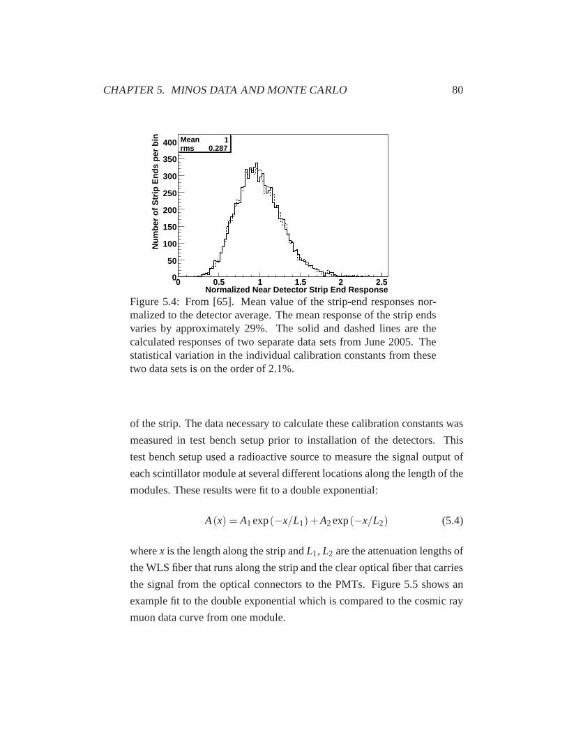
CHAPTER 5. MINOS DATA AND MONTE CARLO 80
Mean 1rms 0.287
Normalized Near Detector Strip End Response0 0.5 1 1.5 2 2.5
Num
ber
of S
trip
End
s pe
r bi
n
0
50
100
150
200
250
300
350
400 Mean 1rms 0.287
Figure 5.4: From [65]. Mean value of the strip-end responsesnor-malized to the detector average. The mean response of the strip endsvaries by approximately 29%. The solid and dashed lines are thecalculated responses of two separate data sets from June 2005. Thestatistical variation in the individual calibration constants from thesetwo data sets is on the order of 2.1%.
of the strip. The data necessary to calculate these calibration constants was
measured in test bench setup prior to installation of the detectors. This
test bench setup used a radioactive source to measure the signal output of
each scintillator module at several different locations along the length of the
modules. These results were fit to a double exponential:
A(x) = A1exp(−x/L1)+A2exp(−x/L2) (5.4)
wherex is the length along the strip andL1, L2 are the attenuation lengths of
the WLS fiber that runs along the strip and the clear optical fiber that carries
the signal from the optical connectors to the PMTs. Figure 5.5 shows an
example fit to the double exponential which is compared to thecosmic ray
muon data curve from one module.

CHAPTER 5. MINOS DATA AND MONTE CARLO 81
Hit Position (m)-2 -1 0 1 2
Ligh
t Out
put
(AD
C)
600
800
1000
1200
1400Cosmic-ray Muon Signal
Fit to Mapper Data
Figure 5.5: From [65]. Comparison of cosmic ray muon data (points)with module mapper fitting results (solid curve) for a typical strip inthe near detector.
• Absolute Energy Scale (M): is a final scale factor that sets the absolute
energy scale of the signal that is recored from the individual strips. The cal-
ibration constant is calculated from the end region of the cosmic ray muons
that stop in the detectors [72]. Stopping the ending parts ofcosmic ray
muons are used because this is the region of muon energy loss that is best
understood. The average response for each strip is calculated, then the mean
value from all the strips defines a muon equivalent unit (MEU).
The final conversion factor converts the energy deposited inthe detector in MEU
into a standard expression of energy the GeV. This needs to bedone separately
for muon tracks, and hadronic and electromagnetic showers.The MEU to GeV
conversion factor for muons, comparisons of the corrected data at the ND and FD
is made to the MC simulation, along with the information on muon stopping power
from [67], this gives a MEU to GeV conversion factor of 2.00±0.02 MeV/MEU.
The results from the CalDet were used to extract a MEU to GeV conversion
factor for electromagnetic and hadronic showers, the CalDet data was compared

CHAPTER 5. MINOS DATA AND MONTE CARLO 82
to the hadronic MC simulations. The combinationGEANT/GCALOR [73] was
found to best describe the CalDet data (shown in Figure 5.6) which agrees with
the data at the 1-5% level. The MEU to GeV conversion factor was determined to
be energy and shower type dependent (hadronic or electromagnetic).
0
5
10 data 0.6 GeV/c
data 1.6 GeV/c
data 3.0 GeV/c
MC
π
0 100 200
0
5
10
15
e
calorimeter signal (a.u.)
% e
vent
s / b
in
Figure 5.6: From [65]. MINOS calorimetric response to pionsandelectrons at three momenta. The calorimeter-signal scale is in arbi-trary units. The data (open symbols), obtained from the calibrationdetector exposure to CERN test beams, are compared to distributionsfrom Monte Carlo simulations.

CHAPTER 5. MINOS DATA AND MONTE CARLO 83
5.2 MINOS MC
MINOS uses a Monte Carlo simulation (MC) to model: the production of hadrons
produced by the 120 GeV protons colliding with the NuNI target, the propagation
of the hadrons off of the NuMI target through the beam system,the production
of the tertiary neutrinos in the NuMI beam, the neutrino interactions within the
Near and Far detectors, and the propagation of the secondaryparticles from the
neutrino interactions through the Near and Far detectors.
The FLUKA05 MC simulates the hadron production off of and through the
NuMI target. The rest of the NuMI beamline is simulated usingtheGEANT-3 [74]
based software packageGNUMI. Every hadronic decay that produce a neutrino is
saved to be used later for the neutrino interaction simulation.
Neutrino scattering off of nuclei within the Near and Far detectors are sim-
ulated by theNEUGEN [33] neutrino event generator. TheNEUGEN simulation
contains descriptions of the dominant neutrino interaction processes that can hap-
pen in the MINOS detectors. These are: quasi-elastic scattering (QE), resonance
production (RES), deep-inelastic scattering (DIS), and coherent pion production
(Coh). TheNEUGEN cross section predictions for some of these interaction pro-
cesses along with data from a few different experiments usedto tuneNEUGEN are
shown in Figure 5.7.
QE scattering is modeled, using the formalism discussed in Chapter 2, with
the BBBA-2005 vector form factors and the dipole form for theaxial-vector form
factor.NEUGEN uses−1.267 forFA(0) and a nominal value of 0.99 GeV for the
axial-vector massMQEA . NEUGEN simulates the effect of the nucleus on the recoil
proton using a RFG model, the RFG model includes the effects of Fermi motion
along with Pauli blocking.
NEUGEN uses the Rein-Seghal [75] model of resonance production anda mod-
ified Bodek-Yang [76] model of DIS interactions. The Bodek-Yang model used by
NEUGEN has been extended to improve the treatment of the resonance to DIS tran-
sition region [77]. For invariant masses less than 2.3 GeV (W < 2.3 GeV) a mod-
ified KNO [78] scaling is used to describe the multiplicity ofthe final state. How-
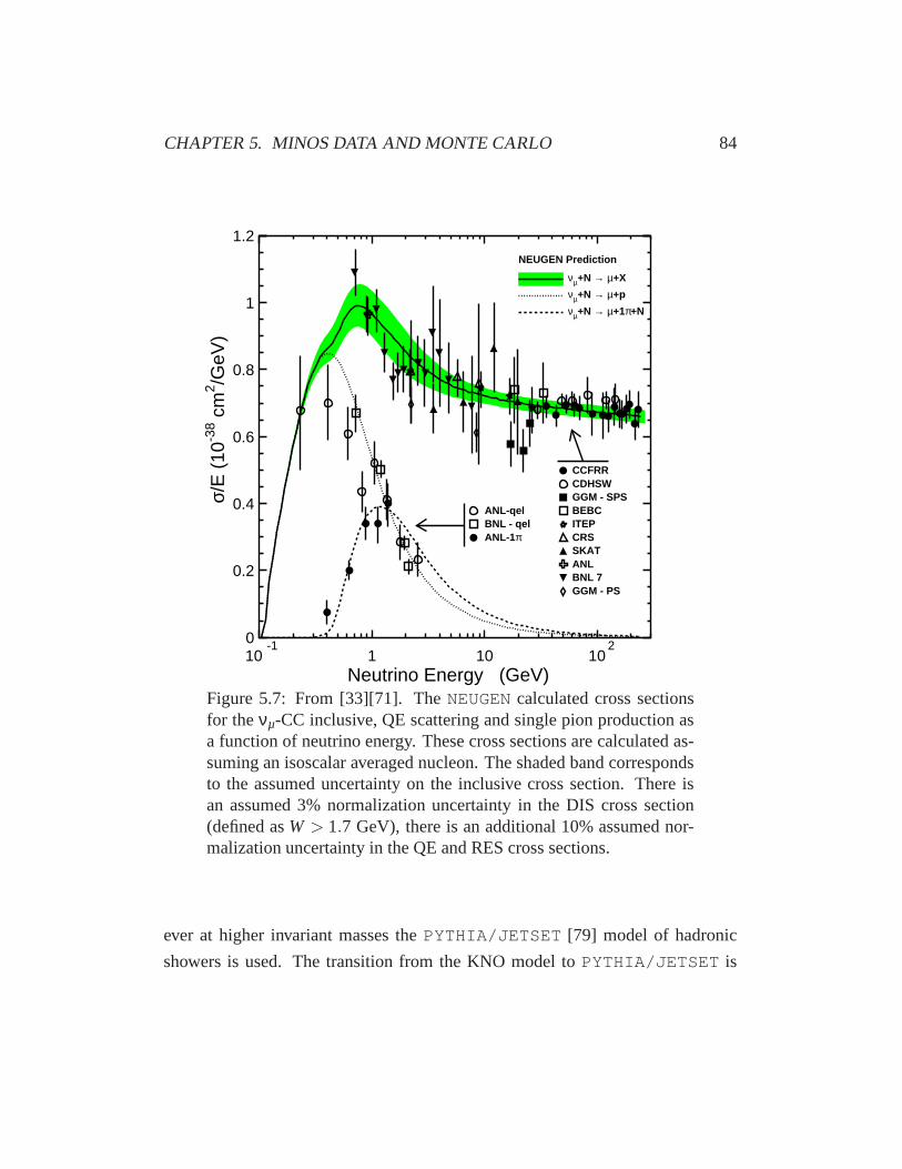
CHAPTER 5. MINOS DATA AND MONTE CARLO 84
0
0.2
0.4
0.6
0.8
1
1.2
10-1
1 10 102
NEUGEN Prediction
νµ+N → µ+X
νµ+N → µ+p
νµ+N → µ+1π+N
BNL 7
CCFRRCDHSWGGM - SPSBEBCITEP
SKATCRS
GGM - PS
ANL
ANL-qelBNL - qelANL-1π
Neutrino Energy (GeV)
σ/E
(10
-38 c
m2 /G
eV)
Figure 5.7: From [33][71]. TheNEUGEN calculated cross sectionsfor theνµ-CC inclusive, QE scattering and single pion production asa function of neutrino energy. These cross sections are calculated as-suming an isoscalar averaged nucleon. The shaded band correspondsto the assumed uncertainty on the inclusive cross section. There isan assumed 3% normalization uncertainty in the DIS cross section(defined asW > 1.7 GeV), there is an additional 10% assumed nor-malization uncertainty in the QE and RES cross sections.
ever at higher invariant masses thePYTHIA/JETSET [79] model of hadronic
showers is used. The transition from the KNO model toPYTHIA/JETSET is
CHAPTER 5. MINOS DATA AND MONTE CARLO 85
done gradually in the invariant mass region of 2.3 < W < 3.0 GeV above which
thePYTHIA/JETSET model is the sole model of hadronic showers.
The MINOS detectors and the most of the NuMI beamline use theGEANT-3
based programGMINOS. The simulation randomly samples the neutrinos that
were saved at theFLUKA05/GNUMI step and propagates them through the MI-
NOS detectors. Neutrino interactions are simulated in bothphysical detectors
and the surrounding rock, the interaction products of neutrino interactions within
the rock are propagated into the physical detectors.GMINOS is interfaced with
NEUGEN, which generates the neutrino interactions. Final state interactions (FSIs)
are modeled inNEUGEN using theINTRANUKE software package [80] [81].
INTRANUKE governs the passage of particles produced in the primary neutrino-
nucleon interaction through the internal structure of the nucleus. The final state
particles generated byNEUGEN are passed back toGMINOS which propagates
the particles through the detectors. Hadronic interactions are simulated using the
GCALOR package. All of the simulated energy depositions are converted into light
signals and electronic signals in the PMTs and front-end electronics. This simu-
lated data is then passed to the MINOS reconstruction in an identical form to the
MINOS data.
5.2.1 Beam Re-Weighting
Neutrinos are created as the result of the decay of pions and kaons within the
NuMI decay pipe. Modeling the correct population of these secondary pions
and kaons in the decay pipe, with the correct momentum is crucial for correctly
modeling the neutrino energy spectrum. Model uncertainties in the production of
these secondary hadrons generate significant uncertainty in the predicted neutrino
flux. Furthermore comparisons between ND data and nominal NDMC simula-
tions demonstrate significant disagreement in the high energy edge of the beam
peak in the LE beam configuration. There is much less disagreement in the same
energy range of other beam configurations. This is evidence that this discrepancy
is not due to mis-modeling of detector acceptance or neutrino cross sections. A

CHAPTER 5. MINOS DATA AND MONTE CARLO 86
beam fitting procedure was implemented to further constrainthe MC simulation,
and thus produce a more accurate neutrino flux prediction [82].
The ND is used to measure the neutrino flux in several different beam con-
figurations, each configuration has a corresponding MC simulation. Table 5.1
contains all of the different beam configurations used in thebeam fit along with
exposure of each configuration. A multi-variable fit of the MCsimulations was
performed until there was good agreement between the fit MC and the recorded
ND data. Penalty terms within the fit were created to constrain theπ+/π− ratio to
theFLUKA05MC simulation along with the NA49 hadron production experiment
[83]. The fit was performed simultaneously on the different beam configurations,
the best fit values were then used to calculate an importance weight for each sim-
ulated neutrino interaction.
Beam Target Horn Peak ExposureConfiguration Position (cm) Current (kA) Eν ± r.m.s (GeV) 1018 GeV
LE010/0kA 10 0 7.4±4.1 2.69LE010/170kA 10 170 3.1±1.1 1.34LE010/185kA 10 185 3.3±1.1 127.0LE010/200kA 10 200 3.5±1.1 1.26LE100/200kA 100 200 5.6±1.5 1.11LE250/200kA 250 200 8.6±2.7 1.55
Table 5.1: The target position refers to the distance the target was dis-placed upstream of its default position inside the rst focusing horn.The peak (i.e., most probable) neutrino energyEν is determined af-ter multiplying the muon-neutrino ux predicted by the beam MonteCarlo simulation by charged-current cross-section. The r.m.s. refersto the root mean square of the peak of the neutrino energy distribu-tion. The 0 kA “horn-off” beam is unfocused and has a broad energydistribution.
The beam tuning procedure uses the BMPT parameterization [84] of hadron
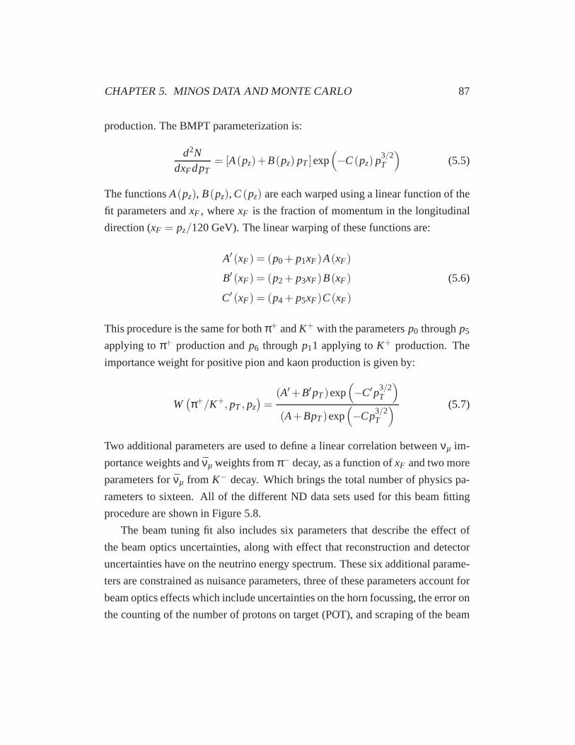
CHAPTER 5. MINOS DATA AND MONTE CARLO 87
production. The BMPT parameterization is:
d2NdxFdpT
= [A(pz)+B(pz) pT ]exp(
−C(pz) p3/2T
)
(5.5)
The functionsA(pz), B(pz), C(pz) are each warped using a linear function of the
fit parameters andxF , wherexF is the fraction of momentum in the longitudinal
direction (xF = pz/120 GeV). The linear warping of these functions are:
A′ (xF) = (p0 + p1xF)A(xF)
B′ (xF) = (p2 + p3xF)B(xF) (5.6)
C′ (xF) = (p4 + p5xF)C(xF)
This procedure is the same for bothπ+ andK+ with the parametersp0 throughp5
applying toπ+ production andp6 throughp11 applying toK+ production. The
importance weight for positive pion and kaon production is given by:
W(
π+/K+, pT , pz)
=(A′+B′pT)exp
(
−C′p3/2T
)
(A+BpT)exp(
−Cp3/2T
) (5.7)
Two additional parameters are used to define a linear correlation betweenνµ im-
portance weights andνµ weights fromπ− decay, as a function ofxF and two more
parameters forνµ from K− decay. Which brings the total number of physics pa-
rameters to sixteen. All of the different ND data sets used for this beam fitting
procedure are shown in Figure 5.8.
The beam tuning fit also includes six parameters that describe the effect of
the beam optics uncertainties, along with effect that reconstruction and detector
uncertainties have on the neutrino energy spectrum. These six additional parame-
ters are constrained as nuisance parameters, three of theseparameters account for
beam optics effects which include uncertainties on the hornfocussing, the error on
the counting of the number of protons on target (POT), and scraping of the beam

CHAPTER 5. MINOS DATA AND MONTE CARLO 88
Neutrino Energy (GeV)
PO
T
16E
vent
s / G
eV /
10
0 5 10 15 20
Dat
a/M
C
1
1.5
10
20
30 LE10/170kA
DataFluka05 MCFull MC Tuning
0 5 10 15 20
Dat
a/M
C
1
1.5
10
20
30
40 LE10/200kA
0 5 10 15 20
Dat
a/M
C
1
1.5
20
40
60
80 LE250/200kA
0 5 10 15 20
Dat
a/M
C
1
1.5
10
20
30
40
Near Detector
LE10/185kA
0 5 10 15 20
Dat
a/M
C
1
1.5
20
40
60
80 LE100/200kA
0 5 10 15 20
Dat
a/M
C
1
1.5
2
4
6 LE10/0kA
Figure 5.8: From [71].νµ charged-current energy spectra measuredin the six beam configurations of Table 5.1 and compared with theMonte Carlo prediction. Two Monte Carlo predictions are shown:one (thin line) with theab initio calculation based onFLUKA05, theother (thick line) after constraining hadron production, focusing anddetector parameters with the neutrino data. Panels along the bottomof each figure show the ratio of the measured and simulated spectra.
along the collimator baffle. The contribution of these parameters to the predicted
neutrino energy spectrum is shown in Figure 5.9. The remaining three parameters
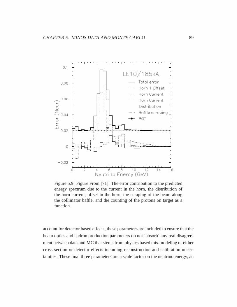
CHAPTER 5. MINOS DATA AND MONTE CARLO 89
Figure 5.9: Figure From [71]. The error contribution to the predictedenergy spectrum due to the current in the horn, the distribution ofthe horn current, offset in the horn, the scraping of the beamalongthe collimator baffle, and the counting of the protons on target as afunction.
account for detector based effects, these parameters are included to ensure that the
beam optics and hadron production parameters do not ‘absorb’ any real disagree-
ment between data and MC that stems from physics based mis-modeling of either
cross section or detector effects including reconstruction and calibration uncer-
tainties. These final three parameters are a scale factor on the neutrino energy, an

CHAPTER 5. MINOS DATA AND MONTE CARLO 90
offset on the hadronic energy scale, and a scale factor on thetrue NC background
that is naturally in the CC selected sample.
Chapter 6
Event Selection
This analysis will measure the axial-vector mass (MQEA ) by fitting the shape of the
Q2 distribution of QE dominated sub-samples of theνµ-CC event sample. Mul-
tiple sub-sample each with different kinematic compositions will be fit simulta-
neously, which will minimize the impact of important detector and physics based
systematics to this analysis.
The event selection procedure is divided into several steps. First a νµ-CC
enhanced (CC-like) event sample is selected. This CC-like event sample is divided
into several different subsamples, these subsamples have different compositions
of the interaction types (QE, RES, DIS).
6.1 νµ-CC Event Selection
The procedure for selectingνµ-CC events is divided into several different sub-
selection criteria. First a number of requirements are imposed that ensure that
a candidate interaction comes from a high-quality neutrinobeam in the proper
configuration. Next additional selection criteria are imposed which ensure that
the interaction originated from a beam neutrino and that allof the information
necessary to properly reconstruct the interaction event was recorded within the
detector. The final selection criteria ensure that the candidate interaction is aνµ-
91

CHAPTER 6. EVENT SELECTION 92
CC interaction, this includes a multivariateνµ-CC identification parameter.
6.1.1 Beam Quality Criteria
The first series of selection criteria are imposed on the dataonly (not on MC)
these selection criteria ensure that a high-quality protonbeam was delivered to
NuMI, and that NuMI is in the proper beam configuration. It is not necessary
to apply these selection criteria to the MC because low quality proton beams are
not simulated in the MC, and the various beam configurations used are simulated
individually.
• Beam Configuration: Only data taken in the LE010185i beam configura-
tion is used to measure the quasi-elastic axial mass parameter in this analy-
sis. Data taken in the other beam configurations listed in Table 5.1 are not
used to extractMQEA The data taken in the other beam configurations are
only used for the beam tuning procedure (Section 5.2.1).
• Beam Spot Position:The position of the beam spot on the target is a good
measure of the stability of the proton beam that is deliveredto NuMI. The
MC does not simulate neutrino interactions that originatedfrom an off-
target beam, thus this cut will also ensure that MC and data originate from
the beam position on the target.
• Horizontal and Vertical Beam Width: The horizontal and vertical beam
width are also good measures of the quality of the proton beamdelivered
to NuMI. The MC does not simulate an increased or reduced beamradius,
thus this selection criteria ensures that the data and MC originate from a
beam with the same horizontal and vertical width.
• Horn Current: The amount of current through the focusing horns effects
the neutrino energy spectrum seen by the ND, thus a check is made that
the correct current is flowing through the horns. Thus selection criteria en-
CHAPTER 6. EVENT SELECTION 93
sures the interaction candidates in the data come from the same underlying
neutrino flux.
There were∼64 million interaction candidates recorded in the MINOS near
detector during the first MINOS run. Of these interaction candidates∼54 million
pass the beam quality criteria. These selection criteria are applied to select a closer
to ideal beam (the MC is generated using an ideal neutrino beam).
6.1.2 Near Detector Event Quality Criteria:
After the beam quality selections have been applied, additional selection criteria
are applied to ensure quality data at the ND. These selectioncriteria ensure that
the ND interaction candidate originated from a beam neutrino, while also ensur-
ing that all of the necessary information to reconstruct theneutrino interaction is
present.
• Coincidence with Spill Trigger: requiring that any candidate neutrino in-
teractions occur in coincidence with the NuMI beam spill ensures that the
majority of cosmic-ray induced muons that pass through the ND are re-
moved. The spill trigger window is 16µs wide starting 2µs before the
recorded spill trigger time and closing 14µs after the spill trigger.
• Near Detector Magnetic Field: a check is made to ensure that the ND
magnetic field coil is active. This selection criteria ensures that the infor-
mation on the curvature of particle tracks is available for analysis.
• Fiducial Volume: the reconstructed event vertex must line within a 1 m di-
ameter cylinder centered around the neutrino beam spot and 4m along the
z-axis of the detector starting 1 m from the front face of the detector stop-
ping 5 m inside the detector. The diameter of the cylinder ensures that for
most neutrino interaction candidates the reconstructed hadronic shower is
fully contained by the ND, and also that charged particles entering through
the detector sides are rejected.
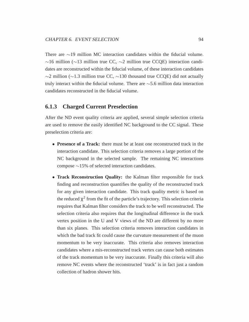
CHAPTER 6. EVENT SELECTION 94
There are∼19 million MC interaction candidates within the fiducial volume.
∼16 million (∼13 million true CC,∼2 million true CCQE) interaction candi-
dates are reconstructed within the fiducial volume, of theseinteraction candidates
∼2 million (∼1.3 million true CC,∼130 thousand true CCQE) did not actually
truly interact within the fiducial volume. There are∼5.6 million data interaction
candidates reconstructed in the fiducial volume.
6.1.3 Charged Current Preselection
After the ND event quality criteria are applied, several simple selection criteria
are used to remove the easily identified NC background to the CC signal. These
preselection criteria are:
• Presence of a Track:there must be at least one reconstructed track in the
interaction candidate. This selection criteria removes a large portion of the
NC background in the selected sample. The remaining NC interactions
compose∼15% of selected interaction candidates.
• Track Reconstruction Quality: the Kalman filter responsible for track
finding and reconstruction quantifies the quality of the reconstructed track
for any given interaction candidate. This track quality metric is based on
the reducedχ2 from the fit of the particle’s trajectory. This selection criteria
requires that Kalman filter considers the track to be well reconstructed. The
selection criteria also requires that the longitudinal difference in the track
vertex position in the U and V views of the ND are different by no more
than six planes. This selection criteria removes interaction candidates in
which the bad track fit could cause the curvature measurementof the muon
momentum to be very inaccurate. This criteria also removes interaction
candidates where a mis-reconstructed track vertex can cause both estimates
of the track momentum to be very inaccurate. Finally this criteria will also
remove NC events where the reconstructed ‘track’ is in fact just a random
collection of hadron shower hits.

CHAPTER 6. EVENT SELECTION 95
• Track Charge Sign: the Kalman filter’s estimate of the track momentum
from curvature is coupled to an estimate of the particles charge. Under the
assumption that the track is produced by a muon, tracks with a‘negative’
curvature are due to negatively charged particles. This selection criteria
requires negative curvature, which will remove both NC interactions can-
didates with a positive pion track and interactions candidates that originate
from νµ-CC interaction.
After applying the charged current preselection criteria∼10.6 million MC in-
teraction candidates remain, of these∼9.6 million are true CC interactions and
∼1.5 million are true CCQE interactions.∼3.6 million data interaction candi-
dates pass the charged current preselection criteria.
6.1.4 νµ-CC Multivariate Identification Parameter
One of the criteria used to select forνµ-CC candidate interactions is a multivari-
ate identification parameter. This identification parameter is calculated using a “k
Nearest-Neighbors” (kNN) algorithm. The kNN algorithmνµ-CC identification
parameter [85] uses the values ofn reconstructed variables from a MC ‘training-
sample’ which contains both information about the reconstructed values and also
information about the “true” interaction. This training sample is used to populate
ann dimensional space of reconstructed quantities that show good discrimination
between charged current interactions and neutral current interactions. A data in-
teraction candidate is placed within then dimensional space and compared to the
k nearest neighbors in then dimensional space. Thesek nearest neighbors “vote”
to classify the test interaction candidate, where the vote is based on the MC truth
of the each of thek nearest neighbors. Thus if the kNN output value is 0.90, then
90% of thek nearest neighbors are trueνµ-CC interactions and voted to classify
the test interaction candidate as aνµ-CC interaction and the remaining 10% of the
k nearest neighbors are true NC interactions and voted to classify the test inter-
action candidate as an NC interaction. The input variables along with the values

CHAPTER 6. EVENT SELECTION 96
k andn where tuned to maximize the product of selection purity and efficiency
where purity and efficiency are defined as:
purity =# True CC Events# Selected Events
(6.1)
efficiency=# Selected CC Events# Total true CC Events
(6.2)
the optimum value fork was found to be 80 nearest neighbors, while the variables
with the greatest distinguishing power are:
• Number of Planes in Interaction Candidate: A νµ-CC interaction will
produce a muon, muons usually have long tracks in the ND. However NC
interactions will only produce a hadronic shower. Hadronicshowers will,
in general, not extend as far in thez-direction as far as muon track will. The
data and MC distribution of this variable is shown in Figure 6.1a.
• Mean Energy Deposited per Strip:defined as the total pulse-height in an
event, measured in MIP, divided by the total number of stripsin the interac-
tion candidate. Muons at MINOS energies are minimum-ionizing particles,
and will have many strip hits with very little energy. Pions,which also inter-
act strongly, will knock out protons as they propagate through the MINOS
detectors. The knocked out protons are not minimum-ionizing particles and
thus will deposit a lot of energy in each strip as the pions pass through. This
variable will thus differentiate NC type interactions fromCC interactions.
The data and MC distributions for this variable are shown in Figure 6.1b.
• Signal Fluctuation Parameter: defined as the number of low pulse-height
strips per high pulse-height strips in and around the track,where high and
low pulse-height are defined relative to the average pulse-height of strips
within the track. Pions are likely to be absorbed by a nucleusat the end
pion track, while this is very rare for muons. The data and MC distributions
for this variable are shown in Figure 6.1c.
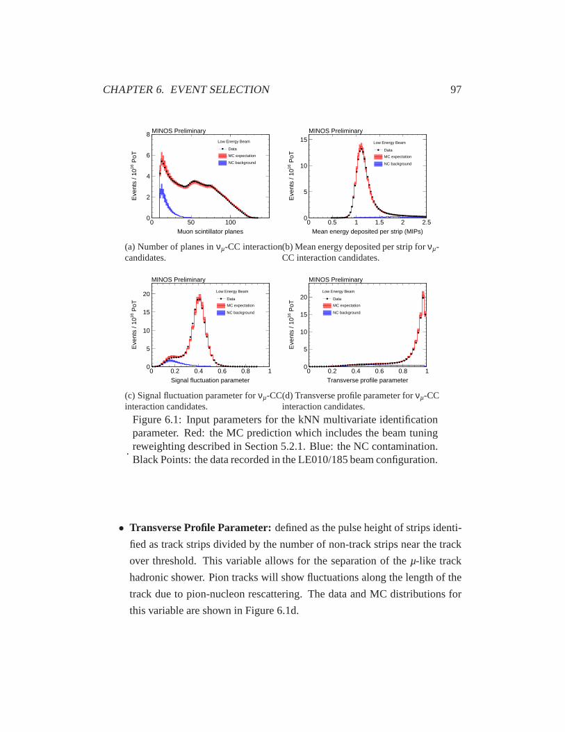
CHAPTER 6. EVENT SELECTION 97
Muon scintillator planes
0 50 100
PoT
16E
vent
s / 1
0
0
2
4
6
8 MINOS Preliminary
Low Energy Beam
Data
MC expectation
NC background
(a) Number of planes inνµ-CC interactioncandidates.
Mean energy deposited per strip (MIPs)
0 0.5 1 1.5 2 2.5
PoT
16E
vent
s / 1
0
0
5
10
15MINOS Preliminary
Low Energy Beam
Data
MC expectation
NC background
(b) Mean energy deposited per strip forνµ-CC interaction candidates.
Signal fluctuation parameter
0 0.2 0.4 0.6 0.8 1
PoT
16E
vent
s / 1
0
0
5
10
15
20
MINOS Preliminary
Low Energy Beam
Data
MC expectation
NC background
(c) Signal fluctuation parameter forνµ-CCinteraction candidates.
Transverse profile parameter
0 0.2 0.4 0.6 0.8 1
PoT
16E
vent
s / 1
0
0
5
10
15
20
MINOS Preliminary
Low Energy Beam
Data
MC expectation
NC background
(d) Transverse profile parameter forνµ-CCinteraction candidates.
.
Figure 6.1: Input parameters for the kNN multivariate identificationparameter. Red: the MC prediction which includes the beam tuningreweighting described in Section 5.2.1. Blue: the NC contamination.Black Points: the data recorded in the LE010/185 beam configuration.
• Transverse Profile Parameter:defined as the pulse height of strips identi-
fied as track strips divided by the number of non-track stripsnear the track
over threshold. This variable allows for the separation of the µ-like track
hadronic shower. Pion tracks will show fluctuations along the length of the
track due to pion-nucleon rescattering. The data and MC distributions for
this variable are shown in Figure 6.1d.

CHAPTER 6. EVENT SELECTION 98
The first 20% of the track is excluded from the calculation of these variables.
This is done to remove most of the noise due to the hadronic shower of the inter-
action candidate. The data and MC distributions for the kNN multivariate iden-
tification variable along with are shown in Figure 6.2. The final νµ-CC selection
criteria requires that the kNN multivariate identificationvariable be greater than
0.3. The finalνµ-CC selection efficiency along with the NC contamination is
shown in Figure 6.3.∼3 million data interaction candidates are selected by this
multivariate identification parameter.
CC/NC separation parameter
0 0.2 0.4 0.6 0.8 1
PoT
16E
vent
s / 1
0
-210
-110
1
10
MINOS Preliminary
Low Energy Beam
Data
MC expectation
NC background
Figure 6.2: the kNN multivariate identification parameter for candi-dateνµ-CC interactions. Red: the MC prediction which includes thebeam tuning reweighting described in Section 5.2.1. Blue: the NCcontamination. Black Points: the data recorded in the LE010/185beam configuration.
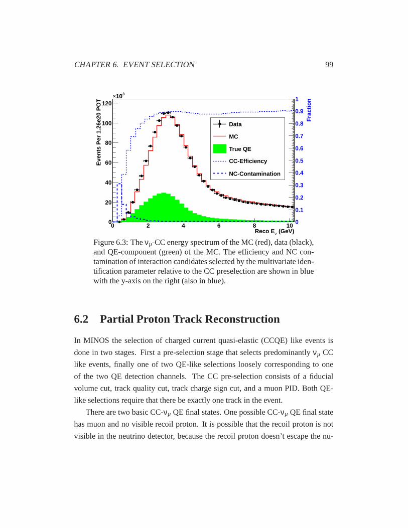
CHAPTER 6. EVENT SELECTION 99
(GeV)ν Reco E0 2 4 6 8 10
Eve
nts
Per
1.2
6e20
PO
T
0
20
40
60
80
100
120
310×
Data
MC
True QE
CC-Efficiency
NC-Contamination
Fra
ctio
n
0
0.1
0.2
0.3
0.4
0.5
0.6
0.7
0.8
0.9
1
Figure 6.3: Theνµ-CC energy spectrum of the MC (red), data (black),and QE-component (green) of the MC. The efficiency and NC con-tamination of interaction candidates selected by the multivariate iden-tification parameter relative to the CC preselection are shown in bluewith the y-axis on the right (also in blue).
6.2 Partial Proton Track Reconstruction
In MINOS the selection of charged current quasi-elastic (CCQE) like events is
done in two stages. First a pre-selection stage that selectspredominantlyνµ CC
like events, finally one of two QE-like selections loosely corresponding to one
of the two QE detection channels. The CC pre-selection consists of a fiducial
volume cut, track quality cut, track charge sign cut, and a muon PID. Both QE-
like selections require that there be exactly one track in the event.
There are two basic CC-νµ QE final states. One possible CC-νµ QE final state
has muon and no visible recoil proton. It is possible that therecoil proton is not
visible in the neutrino detector, because the recoil protondoesn’t escape the nu-

CHAPTER 6. EVENT SELECTION 100
cleus or because the proton has energy below the energy threshold of the detector.
The other CC-νµ QE final state contains both a visible muon and recoil proton.
This analysis will define two sub-samples of theνµ CC sample each composed
primarily of one of these CC-νµ QE final states.
6.2.1 Reconstruction Algorithm
The standard MINOS reconstruction only reconstructs tracks that pass through
5 planes, which translates to a minimum proton kinetic energy of 2.5 GeV. The
typical energy of a QE recoil proton is less than 2 GeV figure (6.4), with most
(95%) of QE interactions having less than 1 GeV this means that the standard
MINOS reconstruction is unable to reconstruct the vast majority of recoil protons
from QE interactions. To use the additional kinematic constraints from the proton
to select QE-like interactions we have developed a new reconstruction algorithm
to reconstruct the recoil proton. Reconstruction of the proton proceeds according
to the following steps.
1. Reconstruct the primary muon track: This is done by the standard MI-
NOS reconstruction.
2. Filter hits from the primary track: When attempting to reconstruct the
potentially very short recoil proton tracks it is necessaryto account for
the possibility that the recoil proton may partially overlap with the recon-
structed muon track. This is done by subtracting the ionization energy of
the muon from the hits on the muon track. Any energy left in anygiven
strip that remains could be from the recoil proton. In MINOS the average
ionization energy of muons has been measured to be 600 sigcor, a quantity
in units of raw ADCs where drift, linearity, and strip to strip corrections
have been applied, but fiber attenuation which is a small effect has not.
3. Filter superfluous hits: In addition to filtering hits that are associated with
the primary track, the algorithm applies two secondary hit filters. The first
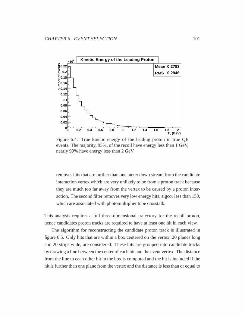
CHAPTER 6. EVENT SELECTION 101
(GeV)P T0 0.2 0.4 0.6 0.8 1 1.2 1.4 1.6 1.8 2
num
ber
of e
vent
s
0
0.02
0.04
0.06
0.08
0.1
0.12
0.14
0.16
0.18
0.2
0.22
610×Mean 0.2783
RMS 0.2946
Kinetic Energy of the Leading Proton
Figure 6.4: True kinetic energy of the leading proton in trueQEevents. The majority, 95%, of the recoil have energy less than 1 GeV,nearly 99% have energy less than 2 GeV.
removes hits that are further than one meter down stream fromthe candidate
interaction vertex which are very unlikely to be from a proton track because
they are much too far away from the vertex to be caused by a proton inter-
action. The second filter removes very low energy hits, sigcor less than 150,
which are associated with photomultiplier tube crosstalk.
This analysis requires a full three-dimensional trajectory for the recoil proton,
hence candidates proton tracks are required to have at leastone hit in each view.
The algorithm for reconstructing the candidate proton track is illustrated in
figure 6.5. Only hits that are within a box centered on the vertex, 20 planes long
and 20 strips wide, are considered. These hits are grouped into candidate tracks
by drawing a line between the center of each hit and the event vertex. The distance
from the line to each other hit in the box is computed and the hit is included if the
hit is further than one plane from the vertex and the distanceis less than or equal to

CHAPTER 6. EVENT SELECTION 102
Z Position (m)5.8 6 6.2 6.4 6.6 6.8 7 7.2 7.4 7.6
Tra
nsve
rse
Pos
ition
(m
)
-0.6
-0.4
-0.2
0
0.2
0.4
0.6
0.8
0
200
400
600
800
1000
1200
1400
1600
Z Position (m)5.8 6 6.2 6.4 6.6 6.8 7 7.2 7.4 7.6
Tra
nsve
rse
Pos
ition
(m
)
-0.6
-0.4
-0.2
0
0.2
0.4
0.6
0.8
0
200
400
600
800
1000
1200
1400
1600
Figure 6.5: Event display of a characteristic true QE event in MINOS.On the top is the full event before any of the hit filters are applied.The plot on the bottom illustrates the grouping algorithm atwork. Inthis case the line is drawn between the event vertex and the red hitthat is in the candidate proton track furthest down stream from theevent vertex. The black boxes represent the regions included in thegrouping algorithm. Any hits whose hit centers are within one of theblack boxes will be counted as part of the candidate proton track.
one strip width or the hit is within one plane and the distanceis less than or equal
to one half a strip width. The final track is the one that has themost hits. After the
track has been formed within the 20 plane by 20 strip box, the 20 plane by 20 strip

CHAPTER 6. EVENT SELECTION 103
restriction is removed and the final line extended out to infinity accumulating hits
that are within one strip. The difference between the reconstructed track direction
and the true proton trajectory is shown in figure 6.6.
(degrees)Candidate/TruePθ∆
0 20 40 60 80 100 120 140 160 180
num
ber
of e
vent
s
0
2
4
6
8
10
310×Mean 15.65
RMS 14.78
Opening Angle Between True Proton and Reconstructed Proton (Selected Events)
(degrees)Candidate/TruePθ∆
0 20 40 60 80 100 120 140 160 180 n
umbe
r of
eve
nts
0
1
2
3
4
5
6
7
8
9310×
Mean 30.53
RMS 27.77
Opening Angle Between True Proton and Reconstructed Proton (True QE Events)
Figure 6.6: Left: The opening angle between the MC true protonmomentum and the reconstructed proton trajectory for all two trackQE selected events. Right: The opening angle between the MC trueproton momentum and the reconstructed proton trajectory for all MCtrue CCQE events with a candidate proton track. The “shoulder” near60◦ in the plot on the right is due to incomplete removal of the muontrack. When there is more than 600 sigcor of pulse height neartheevent vertex, and the true proton is below detection threshold, it ispossible for this algorithm to get confused and interpret the remain-ing muon hits as coming from a proton. This effect is illustrated inFigure 6.5. In the bottom panel of Figure 6.5 there are clearly twohits that were left over from the muon track. It is these hits that couldpotentially confuse this algorithm and create this shoulder.
No attempt is made to reconstruct either the momentum or the energy of the
candidate proton track, only the direction. In addition, the number of hits and
their total pulse height, the total length of the candidate proton track, the number
of planes between the highest pulse height and the furthest downstream hit in the
proton candidate, and the number of unused hits in the vertexhadron shower with
their total pulse height are also recorded.
CHAPTER 6. EVENT SELECTION 104
In QE interactions the recoil proton kinematics is known given the full muon
kinematics and the neutrino beam direction. In this analysis, the reconstructed
muon kinematics and the known beam direction are used to predict the recoil
proton direction using a QE assumption and compared to the direction of the re-
constructed candidate proton track. The comparison is doneby calculating the
opening angle,∆θp, between these two vectors. True QE interactions should pile
up near∆θp of zero. However due to detector resolution and solid angle effects
the peak of this distribution for true QE interactions will be at low angle and not
necessarily peaked at zero.
6.3 The Interaction Sub-Sample Selections
A preselection criteria is applied to theνµ-CC event sample. These preselection
criteria remove obvious non quasi-elastic interactions such as DIS interactions
with very large hadronic showers. This preselection criteria also removes all can-
didate interactions in which the muon track is not fully contained within the ND.
These selection criteria are:
• Single Track: the number of reconstructed tracks in the interaction candi-
date is required to be exactly one. This selection criteria removes candidate
interactions that are obviously not quasi-elastic, such asDIS interactions
with very energetic hadron showers. Energetic hadron showers are more
likely to have additional energetic particles that producesecondary muon-
like tracks. The selection removes such events.
• Interaction Time Window: the high interaction rate at the MINOS ND
can cause multiple neutrino interactions to overlap in the same region of the
detector at the same time. When this happens it becomes very difficult sep-
arating the different interactions into different interaction candidates. The
solution is to require that the separation in between different interaction
candidates be greater than 70 ns.
CHAPTER 6. EVENT SELECTION 105
• Stopping Muons: because the momentum resolution on muons that stop
in the ND is better than the momentum resolution on muons thatexit the
detector. The resolution is better on stopping muons because the momentum
can be measured from the track range which has better resolution than the
momentum measured from curvature.
∼2 million data interaction candidates are retained by the sub-sample preselection
criteria.
Once the preselection criteria has been applied the remaining interaction can-
didates are divided into four different sub-samples of interactions candidates.
These sub-samples of theνµ-CC stopping muon sample are: the low hadronic
energy quasi-elastic like sample, the two track quasi-elastic like sample, the two
track background like sample, and an additional sub-samplewhich consists of in-
teraction candidates that fail to be classified in either of the other sub-samples, the
final event sub-sample is not used in this analysis. When discussing the properties
of these sub-samples it is useful to define the interaction type efficiency and purity
these are defined as:
purity =# True Itype Events
# Selected Events(6.3)
efficiency=# Selected True Itype Events
# Total True Itype Events In CC Sample(6.4)
where Itype is one of the possible interaction types (QE, RES, DIS, Coh).
6.3.1 Low Hadronic Energy Quasi-Elastic Like Selection
This selection is dominated byνµ-CC QE interactions with only muons in the
final state. This sub-sample contains most of the true quasi-elastic interactions
within theνµ-CC sample. However this sub-sample is also dominated by quasi-
elastic interactions in the lowerQ2 region where nuclear effects dominate. This
sample is primarily used to constrain the lowQ2 region behavior of the true quasi-
elastic interactions, though this sub-sample does have some sensitivity to theMQEA
parameter in the higherQ2 region. The selection requirement for this sub-sample

CHAPTER 6. EVENT SELECTION 106
is:
• Reconstructed Hadronic Shower Energy:vertex shower energy less than
250 MeV. Three different types of neutrino interactions make up the major-
ity of all theνµ-CC interactions these are the QE, RES, and DIS interactions
(with a very small contribution form Coh). When consideringthese inter-
actions at the neutrino generator level, they can be defined by considering
the multiplicity of the final state, where QE interactions will produce just a
single proton, RES interactions will produce a proton and a pion, and DIS
interactions will potentially have many protons and pions.Thus QE inter-
actions will leave the least amount of energy (on average) than these other
interaction types. Figure 6.7 shows the reconstructed vertex shower energy.
This Figure demonstrates the region below 250 MeV is dominated by QE
interactions.
Reconstructed Hadronic Shower Energy (GeV) 0 0.1 0.2 0.3 0.4 0.5 0.6 0.7 0.8 0.9 1
Eve
nts
per
1.26
e20
310
410
510
Data Total MC
True Res True QE
Shower Energy
Reconstructed Hadronic Shower Energy (GeV) 0 0.1 0.2 0.3 0.4 0.5 0.6 0.7 0.8 0.9 1
data
/mc
0.8
0.9
1
1.1
1.2
1.3
1.4Shower Energy
Figure 6.7: The reconstructed hadronic shower energy of theneu-trino event. The histograms show the dominant NEUGEN interac-tion types. The event is flagged as QE like if the the reconstructedhadronic shower energy is less than 0.25 GeV

CHAPTER 6. EVENT SELECTION 107
6.3.2 Two Track Quasi-Elastic Like Selection
This sub-sample is dominated by QE interactions with highervalues ofQ2. This
sub-sample has very little true QE interactions within the low Q2 region, thus this
sample has little sensitivity to the nuclear effects that dominate the lowQ2 region.
This selection provides most of the sensitivity to the axial-vector mass parameter,
due to higher QE purity of the sample at higherQ2.
• Reconstructed Hadronic Shower Energy:vertex shower energy greater
than 250 MeV. The intent of these sup-samples is to divide thepreselected
νµ-CC sample in several different exclusive sub-samples. This selection cri-
teria ensures that there are no interaction candidates fromthe low hadronic
energy QE-like selection.
• ∆θp < 30◦
• Number of unused hits< 6: Require that the number of hits in the ver-
tex hadron shower that are not used in the candidate proton track must be
less than 6. QE events should have very little vertex activity outside of the
activity due to the muon track and the proton track.
• Energy profile consistent with proton: Require that the maximum pulse
height hit of the candidate proton track be within one plane of the furthest
downstream hit. Protons lose their energy very rapidly at the end of their
track, this selection criteria looks for the signature of rapid energy loss at
the end of the proton track.
6.3.3 Two Track Background Like Selection
This sub-sample is dominated by resonance interactions andis used to constrain
the resonance background to the QE dominated sample. Even though this sub-
sample is not dominated by QE interactions theQ2 distribution is reconstructed
using the QE assumption as Equation 2.38 instead of an alternativeQ2 calculation
CHAPTER 6. EVENT SELECTION 108
that may be more precise. The QE assumptionQ2 calculation is used because it is
important to accurately model this mis-calculation of the non-QE background to
the QE selections.
• Reconstructed Hadronic Shower Energy:vertex shower energy greater
than 250 MeV. The intent of these sup-samples is to divide thepreselected
νµ-CC sample in several different exclusive sub-samples. This selection cri-
teria ensures that there are no interaction candidates fromthe low hadronic
energy QE-like selection.
• ∆θp cut: if the number of unused hits is less than 6, require that the trajec-
tory of the proton predicted from muon kinematics be furtherthan 30 de-
grees away from the candidate proton track. On occasion one of the∆(1232)
decay products is below the threshold of the detector. When this happens
the number of unused hits may pass in to the range of the QE-like cuts.
These events can be recovered by keep events previously removed by the
QE-like∆θp cut.
• Number of unused hits< 13: require that the number of hits in the vertex
hadronic shower that are not used in the candidate proton track be less than
13. The QE background is dominated by decays of∆(1232) resonances.
The∆(1232) will decay to a nucleon and a pion, because the∆(1232) decays
to two particles, resonance events will leave additional hits in the vertex
hadronic shower.
• Energy profile consistent with proton: Require that the maximum pulse
height hit of the candidate proton track be within one plane of the furthest
downstream hit. Protons lose their energy very rapidly at the end of their
track, this cut looks for that signature.

CHAPTER 6. EVENT SELECTION 109
6.3.4 Selection Purity and Efficiency
There are three different event selections outlined above.Each enhances differ-
ent interaction types, and with different kinematic characteristics. Because this
analysis will be extracting a value forMQEA by simultaneously fitting theQ2 dis-
tribution of all three of these selections, it is important to understand how well
the different interaction types are enhanced within each ofthese event selections
as well as understanding how efficiently the interaction types are selected, all as a
function ofQ2. Figure 6.8 shows the fraction of true QE interactions in each of the
selections and each selections efficiency at selecting trueQE interactions. Figure
6.9 shows the fraction of true resonance interactions in each of the selections and
each selections efficiency at selecting true resonance interactions.
)2 (GeVQE2Q
0 0.5 1 1.5 2 2.5 30
0.1
0.2
0.3
0.4
0.5
0.6
0.7
0.8
0.9
11 Track QE-Like
2 Track QE-Like
2 Track Res-Like
1 Track Fit Region
QE Fraction
)2 (GeVQE2Q
0 0.5 1 1.5 2 2.5 30
0.1
0.2
0.3
0.4
0.5
0.6
0.7
0.8
0.9
11 Track QE-Like
2 Track QE-Like
2 Track Res-Like
1 Track Fit Region
QE Efficiency
Figure 6.8: Left: The fraction of true QE interactions in thegivenselection. Right: The efficiency of selecting true QE interactions rel-ative to the number of true QE interactions in theνµ-CC selection.The one track QE selection is in black, the two track QE is blue, andthe two track background selection is red.
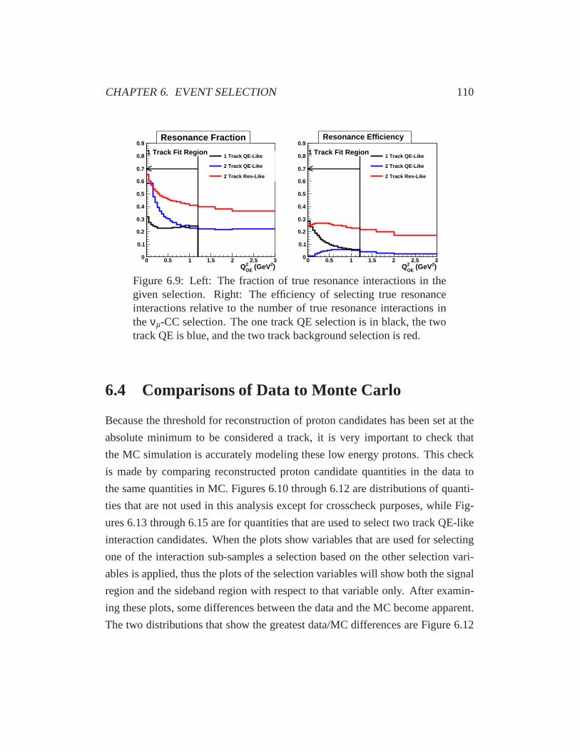
CHAPTER 6. EVENT SELECTION 110
)2 (GeVQE2Q
0 0.5 1 1.5 2 2.5 30
0.1
0.2
0.3
0.4
0.5
0.6
0.7
0.8
0.9
1 Track QE-Like
2 Track QE-Like
2 Track Res-Like
1 Track Fit Region
Resonance Fraction
)2 (GeVQE2Q
0 0.5 1 1.5 2 2.5 30
0.1
0.2
0.3
0.4
0.5
0.6
0.7
0.8
0.9
1 Track QE-Like
2 Track QE-Like
2 Track Res-Like
1 Track Fit Region
Resonance Efficiency
Figure 6.9: Left: The fraction of true resonance interactions in thegiven selection. Right: The efficiency of selecting true resonanceinteractions relative to the number of true resonance interactions intheνµ-CC selection. The one track QE selection is in black, the twotrack QE is blue, and the two track background selection is red.
6.4 Comparisons of Data to Monte Carlo
Because the threshold for reconstruction of proton candidates has been set at the
absolute minimum to be considered a track, it is very important to check that
the MC simulation is accurately modeling these low energy protons. This check
is made by comparing reconstructed proton candidate quantities in the data to
the same quantities in MC. Figures 6.10 through 6.12 are distributions of quanti-
ties that are not used in this analysis except for crosscheckpurposes, while Fig-
ures 6.13 through 6.15 are for quantities that are used to select two track QE-like
interaction candidates. When the plots show variables thatare used for selecting
one of the interaction sub-samples a selection based on the other selection vari-
ables is applied, thus the plots of the selection variables will show both the signal
region and the sideband region with respect to that variableonly. After examin-
ing these plots, some differences between the data and the MCbecome apparent.
The two distributions that show the greatest data/MC differences are Figure 6.12

CHAPTER 6. EVENT SELECTION 111
which shows the distribution of the length of the candidate proton track and Fig-
ure 6.15 which shows the distribution of∆θp. In Figure 6.6 the shoulder in the
true QE distribution in the 60-80 degree range is due to the proton reconstruction
algorithm finding the remains of the muon track instead of therecoil proton. This
region is also the source of major disagreement between dataand MC. There are
significantly more interaction candidates with excess energy very near the muon
track in the data than in the MC. The physics implications of this data/MC differ-
ence is the topic of the Section 6.4.1. The data/MC differences in the track length
could be due to strip to strip alignment; in the MC simulationthe alignment is
known perfectly and exactly matches the design, while real detector is aligned to
±1 mm [86].
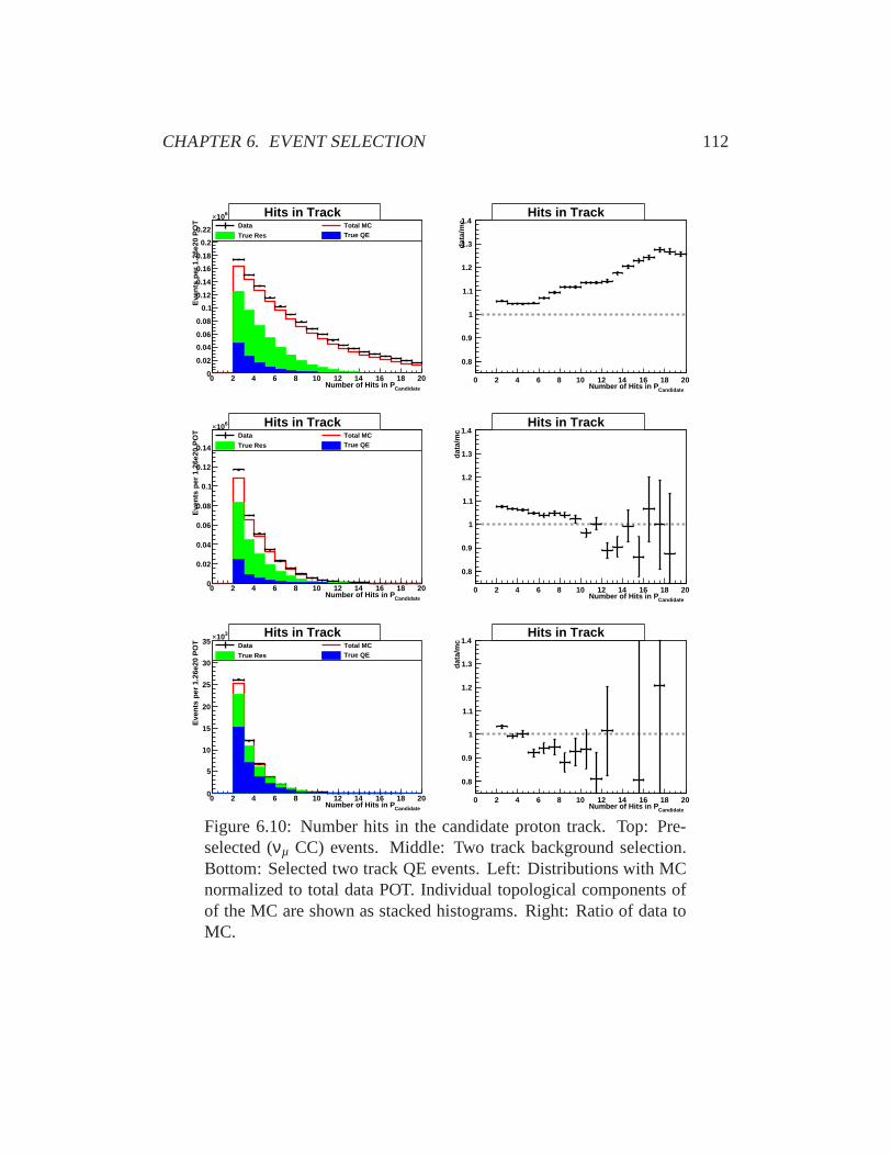
CHAPTER 6. EVENT SELECTION 112
Candidate Number of Hits in P0 2 4 6 8 10 12 14 16 18 20
Eve
nts
per
1.26
e20
PO
T
0
0.02
0.04
0.06
0.08
0.1
0.12
0.14
0.16
0.18
0.2
0.22
610×Data Total MC
True Res True QE
Hits in Track
Candidate Number of Hits in P0 2 4 6 8 10 12 14 16 18 20
data
/mc
0.8
0.9
1
1.1
1.2
1.3
1.4Hits in Track
Candidate Number of Hits in P0 2 4 6 8 10 12 14 16 18 20
Eve
nts
per
1.26
e20
PO
T
0
0.02
0.04
0.06
0.08
0.1
0.12
0.14
610×Data Total MC
True Res True QE
Hits in Track
Candidate Number of Hits in P0 2 4 6 8 10 12 14 16 18 20
data
/mc
0.8
0.9
1
1.1
1.2
1.3
1.4Hits in Track
Candidate Number of Hits in P0 2 4 6 8 10 12 14 16 18 20
Eve
nts
per
1.26
e20
PO
T
0
5
10
15
20
25
30
35310×
Data Total MC
True Res True QE
Hits in Track
Candidate Number of Hits in P0 2 4 6 8 10 12 14 16 18 20
data
/mc
0.8
0.9
1
1.1
1.2
1.3
1.4Hits in Track
Figure 6.10: Number hits in the candidate proton track. Top:Pre-selected (νµ CC) events. Middle: Two track background selection.Bottom: Selected two track QE events. Left: Distributions with MCnormalized to total data POT. Individual topological components ofof the MC are shown as stacked histograms. Right: Ratio of data toMC.

CHAPTER 6. EVENT SELECTION 113
Energy (sigcor) candidate P0 1 2 3 4 5 6 7 8 9 10
310×
Eve
nts
per
1.26
e20
PO
T
0
2
4
6
8
10
12
14
16
18
20
310×Data Total MC
True Res True QE
Summed Proton Pulse Hight
Energy (sigcor) candidate P0 1000 2000 3000 4000 5000 6000 7000 8000 9000 10000
data
/mc
0.8
0.9
1
1.1
1.2
1.3
1.4Summed Proton Pulse Hight
Energy (sigcor) candidate P0 2 4 6 8 10
310×
Eve
nts
per
1.26
e20
PO
T
0
2
4
6
8
10310×
Data Total MC
True Res True QE
Summed Proton Pulse Hight
Energy (sigcor) candidate P0 2000 4000 6000 8000 10000
data
/mc
0.8
0.9
1
1.1
1.2
1.3
1.4Summed Proton Pulse Hight
Energy (sigcor) candidate P0 2 4 6 8 10
310×
Eve
nts
per
1.26
e20
PO
T
0
0.2
0.4
0.6
0.8
1
1.2
1.4
1.6
1.8
2
2.2
310×Data Total MC
True Res True QE
Summed Proton Pulse Hight
Energy (sigcor) candidate P0 2000 4000 6000 8000 10000
data
/mc
0.8
0.9
1
1.1
1.2
1.3
1.4Summed Proton Pulse Hight
Figure 6.11: Summed pulse height of the scintillator stripsin the can-didate proton track. Top: Pre-selected (νµ CC) events. Middle: Twotrack background selection.Bottom: Selected two track QE events.Left: Distributions with MC normalized to total data POT. Individ-ual topological components of of the MC are shown as stacked his-tograms. Right: Ratio of data to MC.
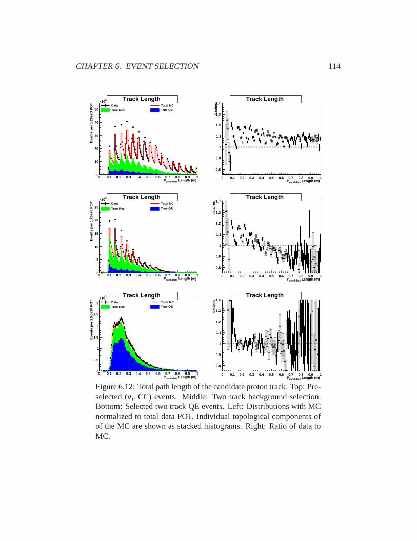
CHAPTER 6. EVENT SELECTION 114
Length (m) candidate P0 0.1 0.2 0.3 0.4 0.5 0.6 0.7 0.8 0.9 1
Eve
nts
per
1.26
e20
PO
T
0
10
20
30
40
50
310×Data Total MC
True Res True QE
Track Length
Length (m) candidate P0 0.1 0.2 0.3 0.4 0.5 0.6 0.7 0.8 0.9 1
data
/mc
0.8
0.9
1
1.1
1.2
1.3
1.4Track Length
Length (m) candidate P0 0.1 0.2 0.3 0.4 0.5 0.6 0.7 0.8 0.9 1
Eve
nts
per
1.26
e20
PO
T
0
5
10
15
20
25
310×Data Total MC
True Res True QE
Track Length
Length (m) candidate P0 0.1 0.2 0.3 0.4 0.5 0.6 0.7 0.8 0.9 1
data
/mc
0.8
0.9
1
1.1
1.2
1.3
1.4Track Length
Length (m) candidate P0 0.1 0.2 0.3 0.4 0.5 0.6 0.7 0.8 0.9 1
Eve
nts
per
1.26
e20
PO
T
0
0.5
1
1.5
2
2.5
3
310×Data Total MC
True Res True QE
Track Length
Length (m) candidate P0 0.1 0.2 0.3 0.4 0.5 0.6 0.7 0.8 0.9 1
data
/mc
0.8
0.9
1
1.1
1.2
1.3
1.4Track Length
Figure 6.12: Total path length of the candidate proton track. Top: Pre-selected (νµ CC) events. Middle: Two track background selection.Bottom: Selected two track QE events. Left: Distributions with MCnormalized to total data POT. Individual topological components ofof the MC are shown as stacked histograms. Right: Ratio of data toMC.
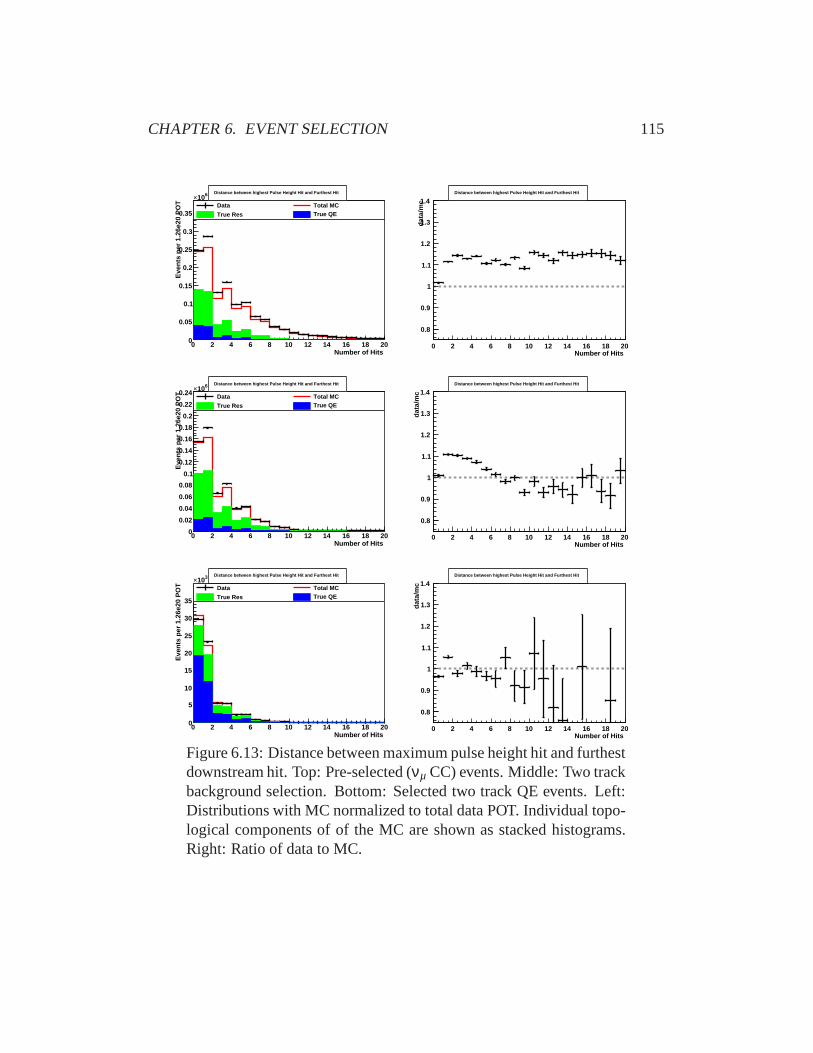
CHAPTER 6. EVENT SELECTION 115
Number of Hits 0 2 4 6 8 10 12 14 16 18 20
Eve
nts
per
1.26
e20
PO
T
0
0.05
0.1
0.15
0.2
0.25
0.3
0.35
610×Data Total MC
True Res True QE
Distance between highest Pulse Height Hit and Furthest Hit
Number of Hits 0 2 4 6 8 10 12 14 16 18 20
data
/mc
0.8
0.9
1
1.1
1.2
1.3
1.4Distance between highest Pulse Height Hit and Furthest Hit
Number of Hits 0 2 4 6 8 10 12 14 16 18 20
Eve
nts
per
1.26
e20
PO
T
0
0.02
0.04
0.06
0.08
0.1
0.12
0.14
0.16
0.18
0.2
0.22
0.24610×
Data Total MC
True Res True QE
Distance between highest Pulse Height Hit and Furthest Hit
Number of Hits 0 2 4 6 8 10 12 14 16 18 20
data
/mc
0.8
0.9
1
1.1
1.2
1.3
1.4Distance between highest Pulse Height Hit and Furthest Hit
Number of Hits 0 2 4 6 8 10 12 14 16 18 20
Eve
nts
per
1.26
e20
PO
T
0
5
10
15
20
25
30
35
310×Data Total MC
True Res True QE
Distance between highest Pulse Height Hit and Furthest Hit
Number of Hits 0 2 4 6 8 10 12 14 16 18 20
data
/mc
0.8
0.9
1
1.1
1.2
1.3
1.4Distance between highest Pulse Height Hit and Furthest Hit
Figure 6.13: Distance between maximum pulse height hit and furthestdownstream hit. Top: Pre-selected (νµ CC) events. Middle: Two trackbackground selection. Bottom: Selected two track QE events. Left:Distributions with MC normalized to total data POT. Individual topo-logical components of of the MC are shown as stacked histograms.Right: Ratio of data to MC.

CHAPTER 6. EVENT SELECTION 116
Number of Unused Shower Hits 0 2 4 6 8 10 12 14 16 18 20
Eve
nts
per
1.26
e20
PO
T
0
10
20
30
40
50
60
70
80
90310×
Data Total MC
True Res True QE
Unused Shower Hits
Number of Unused Shower Hits 0 2 4 6 8 10 12 14 16 18 20
data
/mc
0.8
0.9
1
1.1
1.2
1.3
1.4Unused Shower Hits
Number of Unused Shower Hits 0 2 4 6 8 10 12 14 16 18 20
Eve
nts
per
1.26
e20
PO
T
0
5
10
15
20
25
30
35
40
45
310×Data Total MC
True Res True QE
Unused Shower Hits
Number of Unused Shower Hits 0 2 4 6 8 10 12 14 16 18 20
data
/mc
0.8
0.9
1
1.1
1.2
1.3
1.4Unused Shower Hits
Number of Unused Shower Hits 0 2 4 6 8 10 12 14 16 18 20
Eve
nts
per
1.26
e20
PO
T
0
2
4
6
8
10
12
14
310×Data Total MC
True Res True QE
Unused Shower Hits
Number of Unused Shower Hits 0 2 4 6 8 10 12 14 16 18 20
data
/mc
0.8
0.9
1
1.1
1.2
1.3
1.4Unused Shower Hits
Figure 6.14: Number of unused hits in the vertex hadronic shower.Top: Pre-selected (νµ CC) events. Middle: Two track background se-lection. Bottom: Selected two track QE events. Left: Distributionswith MC normalized to total data POT. Individual topological com-ponents of of the MC are shown as stacked histograms. Right: Ratioof data to MC.

CHAPTER 6. EVENT SELECTION 117
(degrees) Pθ∆ 0 20 40 60 80 100 120 140 160 180
Eve
nts
per
1.26
e20
PO
T
0
5
10
15
20
25
310×Data Total MC
True Res True QE
candidate
and PQE
Opening Angle Between Predicted P
(degrees) Pθ∆ 0 20 40 60 80 100 120 140 160 180
data
/mc
0.8
0.9
1
1.1
1.2
1.3
1.4
candidate and P
QEOpening Angle Between Predicted P
(degrees) Pθ∆ 0 20 40 60 80 100 120 140 160 180
Eve
nts
per
1.26
e20
PO
T
0
1
2
3
4
5
6
310×Data Total MC
True Res True QE
candidate
and PQE
Opening Angle Between Predicted P
(degrees) Pθ∆ 0 20 40 60 80 100 120 140 160 180
data
/mc
0.8
0.9
1
1.1
1.2
1.3
1.4
candidate and P
QEOpening Angle Between Predicted P
(degrees) Pθ∆ 0 20 40 60 80 100 120 140 160 180
Eve
nts
per
1.26
e20
PO
T
0
0.5
1
1.5
2
2.5
3
3.5
310×Data Total MC
True Res True QE
candidate
and PQE
Opening Angle Between Predicted P
(degrees) Pθ∆ 0 20 40 60 80 100 120 140 160 180
data
/mc
0.8
0.9
1
1.1
1.2
1.3
1.4
candidate and P
QEOpening Angle Between Predicted P
Figure 6.15: Opening angle between the candidate proton track andthe proton trajectory predicted from muon kinematics (∆θp). Top:Pre-selected (νµ CC) events. Middle: Two track background selec-tion. Bottom: Selected two track QE events. Left: Distributions withMC normalized to total data POT. Individual topological componentsof of the MC are shown as stacked histograms. Right: Ratio of datato MC.

CHAPTER 6. EVENT SELECTION 118
6.4.1 Nuclear Correlations in MINOS
MINOS is a coarse grained tracking detector, but as has been shown earlier in this
document MINOS has the ability to partially reconstruct therecoil proton inνµ
CCQE interactions. However, the secondary nucleon of an SRCtype interaction
is unlikely to be reconstructable in MINOS, because the secondary nucleon has
a much lower energy than the primary recoil nucleon. While itisn’t possible to
identify SRC type interactions on an event by event basis in MINOS, we can look
for differences between data and the MC prediction of distributions that describe
the activity in the first few strips near the event vertex which would be impacted
by the presence of SRC.
In the QE selected plots of∆θp in Figure 6.15 there is a deficit in the MC
compared to the data in the 60 to 90 degree region. This regionis where the
proton finding algorithm picks up the remnants of the muon track instead of the
proton track. This deficit in the MC prediction implies that the muon track is
not removed as cleanly in the data as it is in the MC. This deficit is because an
occasional event has excess energy very near the muon that doesn’t get subtracted
from the muon track when the muon hits are filtered out of the event. The excess
energy near the vertex may be due to the energy of the secondary nucleon from an
SRC type interaction. If the excess energy near the muon track is due to an extra
nucleon from an SRC type interaction than we should see a difference in the shape
between the data and the MC in the total energy that isn’t accounted for in either
the candidate proton track or the muon track. Under an SRC assumption events
with ∆θp greater than 30◦ should have large amounts of excess energy which is
not accounted for in either the muon track or the proton track. This excess energy
would not appear in the∆θp less than 30◦ sample. The distribution of the excess
energy is shown in Figure 6.16 where the MC exhibits a deficit relative to the data
consistent with the pattern suggested by SRC. The MC deficit extends up to 2000
sigcor (3.2 MIPs) which is a substantial amount of energy. Itseems unlikely that
this could be due mis-modeled detector effects.

CHAPTER 6. EVENT SELECTION 119
Energy (sigcor) 0 1 2 3 4 5
310×
Eve
nts
per
1.26
e20
0
5
10
15
20
25
30
35310×
Data Total MC
True Res True QE
Total PH that is not used in either the Candidate Proton Track and the Muon Track
Energy (sigcor) 0 1000 2000 3000 4000 5000
data
/mc
0.8
0.9
1
1.1
1.2
1.3
1.4Total PH that is not used in either the Candidate Proton Track and the Muon Track
Energy (sigcor) 0 1 2 3 4 5
310×
Eve
nts
per
1.26
e20
0
1
2
3
4
5
6
7
8
310×Data Total MC
True Res True QE
Total PH that is not used in either the Candidate Proton Track and the Muon Track
Energy (sigcor) 0 1000 2000 3000 4000 5000
data
/mc
0.8
0.9
1
1.1
1.2
1.3
1.4Total PH that is not used in either the Candidate Proton Track and the Muon Track
Figure 6.16: Summed pulse height in sigcor of all of the hits that arenot used in either the muon track or the candidate proton track. Top:∆θp sideband selections (QE-like except∆θp > 30). Bottom: Se-lected two track QE events. Left: Distributions with MC normalizedto total data POT. Individual topological components of of the MC areshown as stacked histograms. Right: Ratio of data to MC. The MCdeficit in the 0-2000 sigcor region of the top plots when consideredalong side the MC deficit in the 60-90 degree region of Figure 6.15is further evidence of a secondary nucleon from an SRC type interac-tion. The extra energy that we are seeing is substantial enough thatadditional quanta seems like a more likely explanation thana mis-modeling of detector effects
.
Chapter 7
Extracting the Axial-Vector Mass
The MINOS CCQE-like sub-samples have a significant contribution from non-
CCQE like interactions, this is unlike the NOMAD and MiniBooNE measure-
ments ofMQEA both of which have a smaller contribution from non-CCQE inter-
actions in their CCQE-like sub-samples. This is further complicated because the
MINOS non-CCQE sub-samples have a significant contributionfrom CCQE in-
teractions. Thus characterizing the background must be done simultaneously with
any measurement ofMQEA . First a Mock Data study was done to demonstrate the
validity and quantify the improvements of a multi sub-sample fit procedure, this
study is presented in Section 7.2. Sections 7.3 and 7.4 document attempted fit
procedures that where unable to simultaneously describe the QE-like sub-samples
and the background-like sub-samples. Finally Section 7.5 implements a method
for simultaneously constraining the background while fitting for theMQEA param-
eter, the fit procedure outlined in Section 7.5 is the procedure used to calculate the
results presented in this dissertation.
7.1 Fitting Procedure and Fit Parameters
The three interaction candidate sub-samples discussed in Section 6.3 are fit simul-
taneously in bins ofQ2QE. Each selection is binned in a slightly different manner.
120

CHAPTER 7. EXTRACTING THE AXIAL-VECTOR MASS 121
The low hadronic energy sub-sample is divided into 18 bins over theQ2QE range
of 0 < Q2QE < 1.2 GeV2. The two track QE sub-sample divided into 20 bins
over theQ2QE range of 0< Q2
QE < 3.0 GeV2, and the two track background sub-
sample is divided into 21 bins also over theQ2QE of 0 < Q2
QE < 3.0 GeV2. The
expected number of interaction candidates for each bin is calculated from the MC
for different values of theMQEA parameter along with some other systematic error
parameters. A modifiedχ2 is performed by minimizing theχ2 function:
χ2MCstats=
nBins
∑i=1
(oi −ei(α1, . . . ,αN))2
oi +Sei(α1, . . . ,αN)+
N
∑j=2
∆α2j
σ2α j
In whichoi is the number of observed events in mock data for bin i,ei(α1, ...,αN)
is the expected number of events in the Monte Carlo for bin i given the fit param-
eters,S is the scale factor applied to normalize the MC histogram andthe penalty
term is computed with∆α j , the shift from nominal for thejth systematic param-
eter, andσα j , the assumed 1σ error on thejth systematic parameter. The first fit
parameterα1 ≡ MQEA and is treated as a free parameter in the fit and does not
influence the penalty term.
In addition to consideringMQEA , the fit also includes some of the following four
systematic parameters that are considered to be the most dominant for a shape-
only fit to Q2QE: The effect of a± 30 % shift toMQE
A parameter in the two track
QE-like sample is shown in Figure 7.1
• Muon energy scale: The muon energy scale is the most prominent sys-
tematic error when fitting forMQEA and it directly affects the calculation of
Q2QE. Given that the uncertainty on the range-based momentum of muons
that stop in the Near Detector is smaller than that for the curvature-based
momentum of muons that exit, only stopping muons are included when
fitting for MQEA . This does not result in a large decrease in QE-like sam-
ple statistics because there are relatively fewer quasielastic interactions in
events with higher energy muons. As such, the assumed one sigma uncer-
tainty in the muon energy for stopping muons is taken to be 2% for the

CHAPTER 7. EXTRACTING THE AXIAL-VECTOR MASS 122
) 2 (GeV2 Reco Q0 0.5 1 1.5 2 2.5 3
Eve
nts
per
1e20
PO
T
0
0.5
1
1.5
2
2.5
3
3.5
310× Two Track QE-Like Selection
Nominal MC
- 30%
+ 30%
Two Track QE-Like Selection
) 2 (GeV2 Reco Q0 0.5 1 1.5 2 2.5 3
Shi
ft/N
omin
alσ
1
0.4
0.6
0.8
1
1.2
1.4
1.6Two Track QE-Like Selection Two Track QE-Like Selection
Figure 7.1: Comparison of the nominal MC to reweighted MC with±30% changes to the value ofMQE
A . Only stopping muon events areincluded in this figure.
purposes of calculating theχ2 penalty term. This uncertainty is driven by
the uncertainty in the thickness of the steel planes in the MINOS detectors
along with the uncertainty in the final stopping location of the muon.The
effect of±2% changes to the muon energy scale on theQ2QE distribution for
the 1 track QE-like sample are illustrated in Figure 7.2.
) 2 (GeV2 Reco Q0 0.5 1 1.5 2 2.5 3
Eve
nts
per
1e20
PO
T
0
5
10
15
20
25
30
35
310× One Track QE-Like Selection
Nominal MC
- 2%
+ 2%
One Track QE-Like Selection
) 2 (GeV2 Reco Q0 0.5 1 1.5 2 2.5 3
Shi
ft/N
omin
alσ
1
0.8
0.85
0.9
0.95
1
1.05
1.1
1.15
1.2One Track QE-Like Selection One Track QE-Like Selection
Figure 7.2: Comparison of the nominal MC to scaled MC with±2%scalings of the muon energy. Only stopping muon events are includedin this figure.
• MMMRESA : This parameter plays a similar role toMQE
A but in the modeling of
resonant interactions. Changes toMRESA will affect both the shape and rate

CHAPTER 7. EXTRACTING THE AXIAL-VECTOR MASS 123
of the resonance production cross section as a function ofQ2. Resonance
events form the dominant background in the QE-like sample (although the
extent to which they can be labeled a background is arguable given that
they are very kinematically similar to the true quasielastic events) and this
parameter assures that the fit does not give a biasedMQEA value due to the
mis-modeling of these events. The standard uncertainty of 15% is used
for this parameter when calculating the penalty termχ2 penalty term. This
value for the uncertainty is driven by the from a global analysis of the res-
onances axial-vector mass. Figure 7.3 shows the effect of changes to this
parameter on the 1 track QE-like sample.
) 2 (GeV2 Reco Q0 0.5 1 1.5 2 2.5 3
Eve
nts
per
1e20
PO
T
0
2
4
6
8
10
12
14
16
18
20
22
310× Two Track Background-Like Selection
Nominal MC
- 15%
+ 15%
Two Track Background-Like Selection
) 2 (GeV2 Reco Q0 0.5 1 1.5 2 2.5 3
Shi
ft/N
omin
alσ
1
0.8
0.85
0.9
0.95
1
1.05
1.1
1.15
1.2Two Track Background-Like Selection Two Track Background-Like Selection
Figure 7.3: Comparison of the nominal MC to reweighted MC with±15% changes to the value ofMRES
A . Only stopping muon events areincluded in this figure.
• Effective low QQQ2QE quasi-elastic suppression (kQE
Fermi): It is expected that
the MC will mis-model the data in the very lowQ2 region due to the poorly
understood contribution of nuclear effects to the CCQE cross section. This
parameter is a scale factor applied to the value of the Fermi momenta (for
either protons or neutrons) used to determine whether a given quasielastic
event is Pauli-blocked. The uncertainty on this parameter is hard to deter-
mine and likely fairly large (at least 20-30%) thus an assumed a 30% error
on this parameter for theχ2 penalty term is used. This value for the uncer-
tainty in this parameter is driven by difference in lowQ2 suppression due
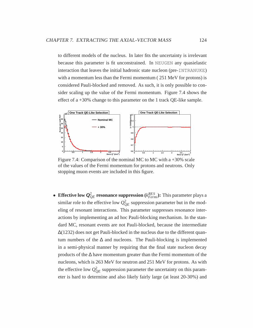
CHAPTER 7. EXTRACTING THE AXIAL-VECTOR MASS 124
to different models of the nucleus. In later fits the uncertainty is irrelevant
because this parameter is fit unconstrained. InNEUGEN any quasielastic
interaction that leaves the initial hadronic state nucleon(pre-INTRANUKE)
with a momentum less than the Fermi momentum ( 251 MeV for protons) is
considered Pauli-blocked and removed. As such, it is only possible to con-
sider scaling up the value of the Fermi momentum. Figure 7.4 shows the
effect of a +30% change to this parameter on the 1 track QE-like sample.
) 2 (GeV2 Reco Q0 0.5 1 1.5 2 2.5 3
Eve
nts
per
1e20
PO
T
0
5
10
15
20
25
30
35
310× One Track QE-Like Selection
Nominal MC
+ 30%
One Track QE-Like Selection
) 2 (GeV2 Reco Q0 0.5 1 1.5 2 2.5 3
Shi
ft/N
omin
alσ
1
0.6
0.7
0.8
0.9
1
1.1
1.2One Track QE-Like Selection One Track QE-Like Selection
Figure 7.4: Comparison of the nominal MC to MC with a +30% scaleof the values of the Fermi momentum for protons and neutrons.Onlystopping muon events are included in this figure.
• Effective low QQQ2QE resonance suppression (kRES
Fermi): This parameter plays a
similar role to the effective lowQ2QE suppression parameter but in the mod-
eling of resonant interactions. This parameter suppressesresonance inter-
actions by implementing an ad hoc Pauli-blocking mechanism. In the stan-
dard MC, resonant events are not Pauli-blocked, because theintermediate
∆(1232) does not get Pauli-blocked in the nucleus due to the different quan-
tum numbers of the∆ and nucleons. The Pauli-blocking is implemented
in a semi-physical manner by requiring that the final state nucleon decay
products of the∆ have momentum greater than the Fermi momentum of the
nucleons, which is 263 MeV for neutron and 251 MeV for protons. As with
the effective lowQ2QE suppression parameter the uncertainty on this param-
eter is hard to determine and also likely fairly large (at least 20-30%) and
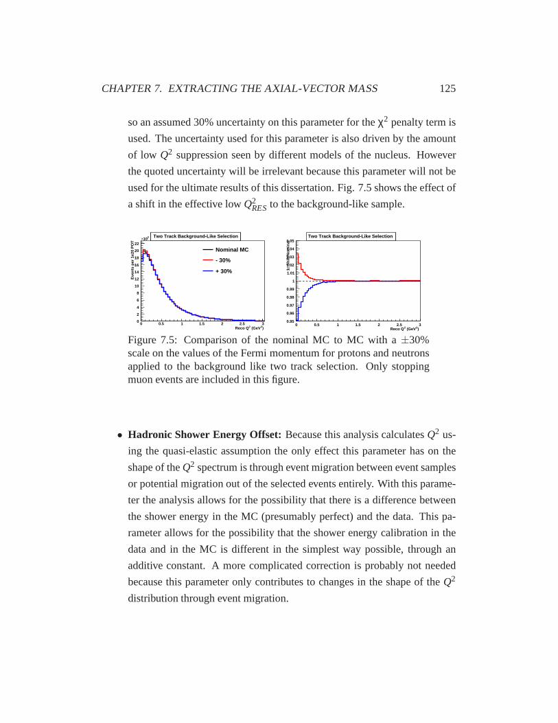
CHAPTER 7. EXTRACTING THE AXIAL-VECTOR MASS 125
so an assumed 30% uncertainty on this parameter for theχ2 penalty term is
used. The uncertainty used for this parameter is also drivenby the amount
of low Q2 suppression seen by different models of the nucleus. However
the quoted uncertainty will be irrelevant because this parameter will not be
used for the ultimate results of this dissertation. Fig. 7.5shows the effect of
a shift in the effective lowQ2RESto the background-like sample.
) 2 (GeV2 Reco Q0 0.5 1 1.5 2 2.5 3
Eve
nts
per
1e20
PO
T
0
2
4
6
8
10
12
14
16
18
20
22
310× Two Track Background-Like Selection
Nominal MC
- 30%
+ 30%
Two Track Background-Like Selection
) 2 (GeV2 Reco Q0 0.5 1 1.5 2 2.5 3
Shi
ft/N
omin
alσ
1
0.95
0.96
0.97
0.98
0.99
1
1.01
1.02
1.03
1.04
1.05Two Track Background-Like Selection Two Track Background-Like Selection
Figure 7.5: Comparison of the nominal MC to MC with a±30%scale on the values of the Fermi momentum for protons and neutronsapplied to the background like two track selection. Only stoppingmuon events are included in this figure.
• Hadronic Shower Energy Offset: Because this analysis calculatesQ2 us-
ing the quasi-elastic assumption the only effect this parameter has on the
shape of theQ2 spectrum is through event migration between event samples
or potential migration out of the selected events entirely.With this parame-
ter the analysis allows for the possibility that there is a difference between
the shower energy in the MC (presumably perfect) and the data. This pa-
rameter allows for the possibility that the shower energy calibration in the
data and in the MC is different in the simplest way possible, through an
additive constant. A more complicated correction is probably not needed
because this parameter only contributes to changes in the shape of theQ2
distribution through event migration.
CHAPTER 7. EXTRACTING THE AXIAL-VECTOR MASS 126
7.2 Mock Data Analysis
There is a total of approximately 725,000 interactions candidates between the
three selections that are used in this analysis. With 46% of the interaction can-
didates in both the low hadronic energy and the two track background-like sub-
samples, the remaining 8% of the interaction candidates arein the two track QE-
like sub-sample. This means that the statistical error in each bin ofQ2 is between
approximately 1 and 2%, making this analysis dominated not by statistical uncer-
tainties but systematic uncertainties in the neutrino interaction models. It is useful
to finalize all of the the major analysis decisions (how many samples,Q2 binning,
goodness of fit metric, etc) before proceeding with the analysis on data this will
limit the impact of selection biases on the final result. Thisis done by analyzing a
mock data sample first. The mock data sample consists of a subset of the MC that
has had the model parameters set to some arbitrary value, while the remaining MC
is then used to attempt to recover the mock data model parameters. The analysis
procedure is tuned to minimize the uncertainty of the mock data analysis while
also minimizing the potential of systematic effects. Once this is done the analysis
is repeated on real data, and potentially changed based on what is learned from
the differences between data and mock data.
7.2.1 Mock Data Construction
The entire MC sample was used to generate a mock dataQ2 distribution for all
three selections. The fit parameters for the mock data distributions were set to the
best fit values for the low hadronic energy analysis that has already been done.
TheseQ2 distributions were then normalized to the run I pot (1.27e20). These
Q2 distributions were then used as a PDF to generate newQ2 distributions with
a number of entries equal to the Poisson fluctuated integral of the original Q2
distributions.

CHAPTER 7. EXTRACTING THE AXIAL-VECTOR MASS 127
7.2.2 Mock Data Fit Results
The fit to the mock data was performed as described in Section 7.1 and generated
as described above in Section 7.1. This fit will be compared tothe fit to only the
low hadronic energy analysis that was presented at the 6th International Work-
shop on Neutrino-Nucleus Interactions in the Few-GeV Region (NuInt09) [87]. A
summary of both of these results are given in Table 7.1, whiletheQ2 distributions
for the mock data fits are shown in Figure 7.6.
Parameter NuInt09 Results Mock Data Study
MQEA (GeV) 1.192 1.17
Eµ−scale 0.988 0.989MRES
A (GeV) 1.112 1.100kQE
F −scale 1.284 1.282kRES
F −scale 1.0 (Fixed) 1.085χ2/ndf 1.023 0.536
Table 7.1: Best fit results and for the two fit configurations and re-ducedχ2 values according to 7.1 for the best fit MC.
The increase in sensitivity from this analysis come from twosources. Break-
ing of correlations between parameters, and different strengths in different kine-
matic regions. The three sub-sample analysis reduces the correlations between
MQEA andkQE
Fermi and also the correlations betweenMQEA andMRES
A . Referring back
to Figure 6.8 the fraction of true QE interactions in the two track QE-like sub-
sample (the blue line from Figure 6.8) shows that there are notrue QE interactions
within the lowQ2 region of this sub-sample, thus any lowQ2 suppression that is
seen in this sub-sample can not be coming from true QE interactions. Further-
more by adding a selection that is dominated by the background to the QE-like
sub-samples, the behavior of the background (as represented by thekRESFermi and
MRESA parameters) in the QE-like sub-samples can be significantlyconstrained.
These additional sub-samples don’t do anything to break thecorrelations between
theEµ−scalehowever because the other selections much more tightly constrain

CHAPTER 7. EXTRACTING THE AXIAL-VECTOR MASS 128
MQEA , theEµ scale is also constrained due to theMQE
A -Eµ correlations.
7.2.3 Conclusion
This mock data study estimates that the three sub-sample fit will reduce by a
factor of 2-3 the impact of the fit error to our measurement of the effectiveMQEA
parameter. And given the impact that other systematics had on the NuInt09 results
the expectation would be that those uncertainties would dominate the uncertainty
of this analysis.
7.3 Initial Fit to Data
Two things were learned from the mock data fit. The mock data fitquantified the
expected improvement to theMQEA measurement from the inclusion of the two,
two track selections, while simultaneously demonstratinghow the fit parameters
are correlated when the fit is performed with multiple sub-samples. Because the
two track selections do a good job of breaking the correlations between,MQEA
andkFermi, andMQEA andMRes
A it becomes possible to fit these parameters uncon-
strained by a penalty term. Thus the first fit to data is performed with all of the
parameters from the mock data fit as free parameters with the exception of the
muon energy scale.
Fit Results
The initial fit to data was performed as described in Section 7.1 with the modifica-
tions outlined in Section 7.3. The resultingQ2QE distributions are shown in Figure
7.8. The best fit values are shown in Table 7.2.
The best fit values for this fit configuration are very different from the best fit
values given by the MINOS NuInt 2009 analysis [87]. Furthermore theχ2 for this
fit configuration is∼18σ from the expected reducedχ2 for a fit with 49 degrees
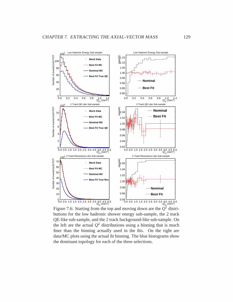
CHAPTER 7. EXTRACTING THE AXIAL-VECTOR MASS 129
) 2 (GeVQE2 Q
0.0 0.2 0.4 0.6 0.8 1.0 1.2
Num
ber
of e
vent
s/1e
20 P
OT
0
20
40
60
80
100
310×
Mock Data
Best Fit MC
Nominal MC
Best Fit True QE
Low Hadronic Energy Sub-sample
) 2 (GeVQE2 Q
0.0 0.2 0.4 0.6 0.8 1.0 1.2
dat
a/M
C
0.80
0.85
0.90
0.95
1.00
1.05
1.10
1.15
Nominal
Best Fit
Low Hadronic Energy Sub-sample
) 2 (GeVQE2 Q
0.0 0.5 1.0 1.5 2.0 2.5 3.0 3.5 4.0 4.5 5.0
Num
ber
of e
vent
s/1e
20 P
OT
0
2
4
6
8
10
310×
Mock Data
Best Fit MC
Nominal MC
Best Fit True QE
2 Track QE-Like Sub-sample
) 2 (GeVQE2 Q
0.0 0.5 1.0 1.5 2.0 2.5 3.0 3.5 4.0 4.5 5.0
dat
a/M
C
0.92
0.94
0.96
0.98
1.00
1.02
1.04 Nominal
Best Fit
2 Track QE-Like Sub-sample
) 2 (GeVQE2 Q
0.0 0.5 1.0 1.5 2.0 2.5 3.0 3.5 4.0 4.5 5.0
Num
ber
of e
vent
s/1e
20 P
OT
0
10
20
30
40
50
60
70
310×
Mock Data
Best Fit MC
Nominal MC
Best Fit True Res
2 Track Resonance-Like Sub-sample
) 2 (GeVQE2 Q
0.0 0.5 1.0 1.5 2.0 2.5 3.0 3.5 4.0 4.5 5.0
dat
a/M
C
0.94
0.96
0.98
1.00
1.02
1.04
1.06
Nominal
Best Fit
2 Track Resonance-Like Sub-sample
Figure 7.6: Starting from the top and moving down are theQ2 distri-butions for the low hadronic shower energy sub-sample, the 2trackQE-like sub-sample, and the 2 track background-like sub-sample. Onthe left are the actualQ2 distributions using a binning that is muchfiner than the binning actually used in the fits. On the right aredata/MC plots using the actual fit binning. The blue histograms showthe dominant topology for each of the three selections.

CHAPTER 7. EXTRACTING THE AXIAL-VECTOR MASS 130
ScaleQEA M
1.10 1.15 1.20 1.25 1.30
Sca
leµ
E
0.980
0.985
0.990
0.995
1.000
MINOS Preliminary
FitHadLow E 3 Selection Fit
Best FitHadLow E 3 Selection Best Fit
Characteristic Mock Data Example
ScaleQEA M
1.10 1.15 1.20 1.25 1.30
Sca
leQ
EF
erm
i k
1.26
1.28
1.30
1.32
1.34
MINOS Preliminary
FitHadLow E 3 Selection Fit
Best FitHadLow E 3 Selection Best Fit
Characteristic Mock Data Example
Figure 7.7: The 1-σ (defined as∆χ2 = 1) contours for the 1 trackNuInt09 analysis and this mock data analysis. The contour for MQE
A
and theEµ− scaleis shown on the left. The contour forMQEA and
kQEFermi− scale is shown on the right. The one track NuInt09 result
contour is shown in red. The contours from this mock data analysisare shown in blue. The three selection analysis significantly improvesthe size of the allowed parameter space. In addition the additionalselections break the correlation betweenMQE
A and thekQEFermi-scale.
Parameter Initial fit to data
MQEA (GeV) 1.000±0.033
Eν −scale 0.992±0.002MRES
A (GeV) 1.078±0.024kQE
F −scale 2.87±0.04kRES
F −scale 1.14±0.01χ2/ndf 2.65
Table 7.2: Best fit values for the fit to data. The errors shown are theMINUIT returned HESSE errors.
of freedom. Thus this fit is a poor description of the data and the best fit values
for the fit parameters are meaningless.
In this fit, the parameterkResFermi has a very different value from the assumed
nominal value of 1. The mock data fit had a assumed one sigma error of 30%, the
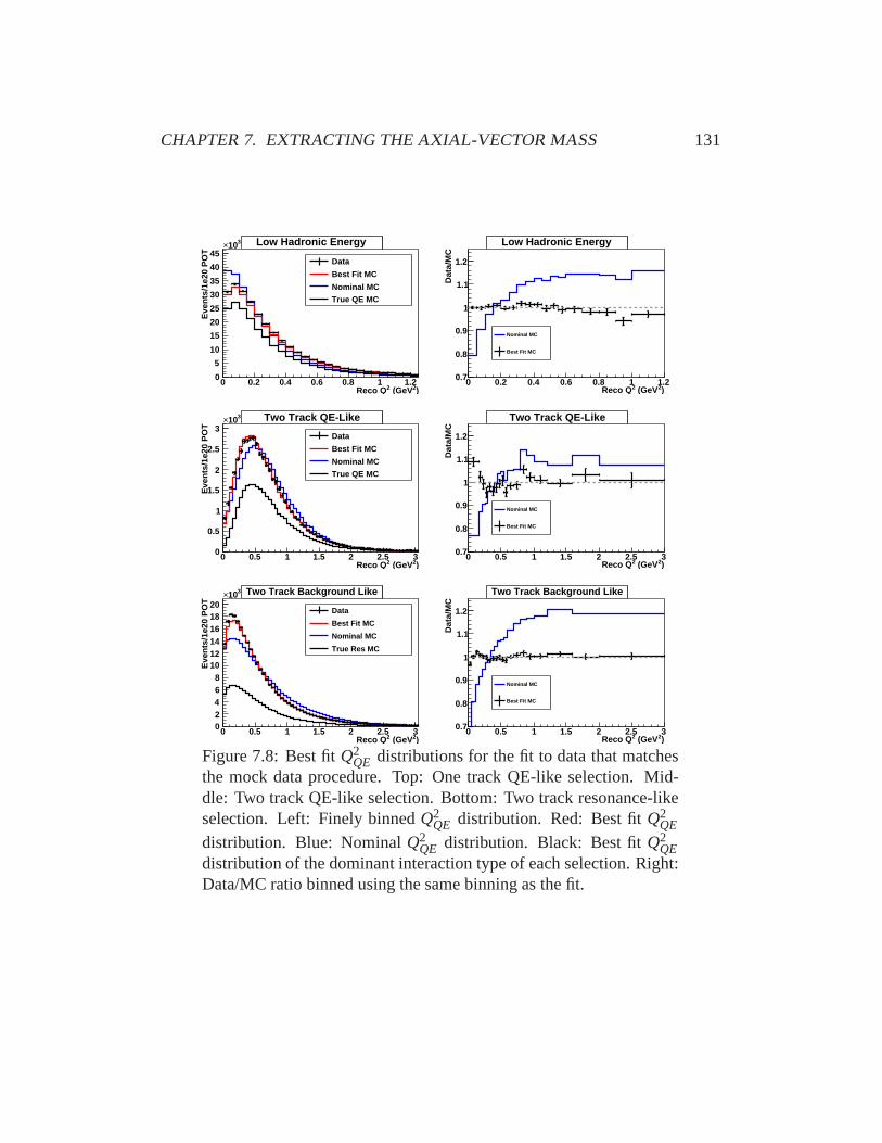
CHAPTER 7. EXTRACTING THE AXIAL-VECTOR MASS 131
)2 (GeV2Reco Q0 0.2 0.4 0.6 0.8 1 1.2
Eve
nts/
1e20
PO
T
0
5
10
15
20
25
30
35
40
45310× Low Hadronic Energy
Data
Best Fit MC
Nominal MC
True QE MC
Low Hadronic Energy
)2 (GeV2Reco Q0 0.2 0.4 0.6 0.8 1 1.2
Dat
a/M
C
0.7
0.8
0.9
1
1.1
1.2
Low Hadronic Energy
Nominal MC
Best Fit MC
Low Hadronic Energy
)2 (GeV2Reco Q0 0.5 1 1.5 2 2.5 3
Eve
nts/
1e20
PO
T
0
0.5
1
1.5
2
2.5
3
310× Two Track QE-Like
Data
Best Fit MC
Nominal MC
True QE MC
Two Track QE-Like
)2 (GeV2Reco Q0 0.5 1 1.5 2 2.5 3
Dat
a/M
C
0.7
0.8
0.9
1
1.1
1.2
Two Track QE-Like
Nominal MC
Best Fit MC
Two Track QE-Like
)2 (GeV2Reco Q0 0.5 1 1.5 2 2.5 3
Eve
nts/
1e20
PO
T
02468
101214161820
310× Two Track Background Like
Data
Best Fit MC
Nominal MC
True Res MC
Two Track Background Like
)2 (GeV2Reco Q0 0.5 1 1.5 2 2.5 3
Dat
a/M
C
0.7
0.8
0.9
1
1.1
1.2
Two Track Background Like
Nominal MC
Best Fit MC
Two Track Background Like
Figure 7.8: Best fitQ2QE distributions for the fit to data that matches
the mock data procedure. Top: One track QE-like selection. Mid-dle: Two track QE-like selection. Bottom: Two track resonance-likeselection. Left: Finely binnedQ2
QE distribution. Red: Best fitQ2QE
distribution. Blue: NominalQ2QE distribution. Black: Best fitQ2
QEdistribution of the dominant interaction type of each selection. Right:Data/MC ratio binned using the same binning as the fit.

CHAPTER 7. EXTRACTING THE AXIAL-VECTOR MASS 132
best fit value here is 6σ away from the mock data fit assumed nominal value. This
kResFermi is suspiciously large, Figure 7.9 compares the nominal resonance MC to
the resonance MC withkQEFermi equal to 2.87. Figure 7.9 demonstrates that even as
high as aQ2QE value of 1, this suppression scheme removes 10% of the resonances
events. The larger than expected suppression of resonance events in the moderate
Q2 region produced bykResFermi equal to 2.87 disagrees with the ad-hoc suppression
function from R. Gran’s and N. Graf’s work in [88].
) 2 (GeV2 Reco Q0 0.5 1 1.5 2 2.5 3
Eve
nts
per
1e20
PO
T
0
1
2
3
4
5
6
310×
Nominal MC
=2.87ResFermik
) 2 (GeV2 Reco Q0 0.5 1 1.5 2 2.5 3
Shi
fted/
Nom
inal
0
0.2
0.4
0.6
0.8
1
1.2
Figure 7.9: Left: true resonanceQ2QE distributions. Blue: distribution
for kResFermi equal to 2.87. Red: nominal true resonanceQ2
QE distri-bution. Right: thekRes
Fermi equal to 2.87 distribution divided by thenominal distribution.
In [88] the authors extract a suppression function for theQ2 distribution of
the resonances using two separate resonance enhanced sub-samples. These event
sub-samples are defined using a simple cut on W, the hadronic invariant mass. The
two selections they define are: The Delta sub-sample defined as W between 0 and
1.3 GeV and the Transition sub-sample defined as W between 1.3and 2.0 GeV.
The Delta sub-sample is dominated by resonances and QE, while the Transition
is dominated by resonances and DIS. Using these two sub-samples the authors
implemented a smoothly shaped suppression function with a shape motivated by
theoretical [89][90] and experimental [34] work on theQ2 shape of resonance
interactions. Using this shape as a starting point the authors then tuned the shape
by reducing the residuals in the Delta and Transition sub-samples to get the final

CHAPTER 7. EXTRACTING THE AXIAL-VECTOR MASS 133
suppression shape shown in Figure 7.10 which is compared to the suppression
that results from akResFermi value of 2.87. By design the suppression function from
[88] turns off forQ2 values greater than 0.6 GeV2, while thekResFermi suppression
in the same region is still about 70%. The natural conclusionfrom the poorχ2
calculated from this fit and the poor agreement between thekResFermi suppression
and the suppression from [88] is that thekResFermi suppression is unphysical.
)2 (GeV2 True Q0 0.5 1 1.5 2 2.5 3
Shi
fted/
Nom
inal
0
0.2
0.4
0.6
0.8
1
1.2
Suppression Function
=2.87ResFermik
)2 (GeV2 True Q0 0.1 0.2 0.3 0.4 0.5 0.6 0.7 0.8 0.9 1
Shi
fted/
Nom
inal
0
0.2
0.4
0.6
0.8
1
1.2
Figure 7.10: Red: suppression function from [88] with errorbandthat includes both statistical and systematic uncertainty. Blue: sup-pression function from akRes
Fermi value of 2.87.
7.4 Fit Using The Resonance Suppression Function
The natural progression from the initial fit to the data is a fitthat incorporates the
resonance suppression function from [88] instead of thekResFermi based suppression.
This fit will use a more realistic suppression function, however the lowQ2 sup-
pression cannot be further tuned to match the data, consequently there is no longer
a parameter that describes the behavior of the lowQ2 resonances interactions. The
resultingQ2 distribution from this fit are shown in Figure 7.11. The best fit values
for the parameters are shown in Table 7.3. This fit has 50 degrees of freedom
instead of 49 because there is one less fit parameter.
This fit with the lowQ2 resonances suppression function is slightly worse than

CHAPTER 7. EXTRACTING THE AXIAL-VECTOR MASS 134
)2 (GeV2Reco Q0 0.2 0.4 0.6 0.8 1 1.2
Eve
nts/
1e20
PO
T
0
5
10
15
20
25
30
35
40
45
310× Low Hadronic Energy
Data
Best Fit MC
Nominal MC
True QE MC
Low Hadronic Energy
)2 (GeV2Reco Q0 0.2 0.4 0.6 0.8 1 1.2
Dat
a/M
C
0.7
0.8
0.9
1
1.1
1.2
Low Hadronic Energy
Nominal MC
Best Fit MC
Low Hadronic Energy
)2 (GeV2Reco Q0 0.5 1 1.5 2 2.5 3
Eve
nts/
1e20
PO
T
0
0.5
1
1.5
2
2.5
3310× Two Track QE-Like
Data
Best Fit MC
Nominal MC
True QE MC
Two Track QE-Like
)2 (GeV2Reco Q0 0.5 1 1.5 2 2.5 3
Dat
a/M
C
0.7
0.8
0.9
1
1.1
1.2
Two Track QE-Like
Nominal MC
Best Fit MC
Two Track QE-Like
)2 (GeV2Reco Q0 0.5 1 1.5 2 2.5 3
Eve
nts/
1e20
PO
T
02468
101214161820
310× Two Track Background Like
Data
Best Fit MC
Nominal MC
True Res MC
Two Track Background Like
)2 (GeV2Reco Q0 0.5 1 1.5 2 2.5 3
Dat
a/M
C
0.7
0.8
0.9
1
1.1
1.2
Two Track Background Like
Nominal MC
Best Fit MC
Two Track Background Like
Figure 7.11: Best fitQ2QE distributions for the fit to data that uses
the lowQ2 suppression function from [88]. Top: One track QE-likeselection. Middle: Two track QE-like selection. Bottom: Two trackresonance-like selection. Left: Finely binnedQ2
QE distribution. Red:Best fit Q2
QE distribution. Blue: NominalQ2QE distribution. Black:
Best fitQ2QE distribution of the dominant interaction type of each se-
lection. Right: Data/MC ratio binned using the same binningas thefit.
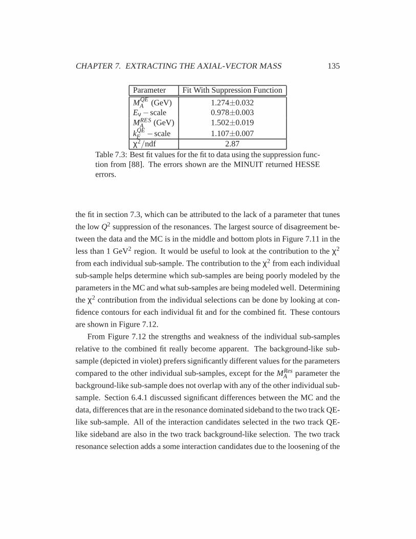
CHAPTER 7. EXTRACTING THE AXIAL-VECTOR MASS 135
Parameter Fit With Suppression Function
MQEA (GeV) 1.274±0.032
Eν −scale 0.978±0.003MRES
A (GeV) 1.502±0.019kQE
F −scale 1.107±0.007χ2/ndf 2.87
Table 7.3: Best fit values for the fit to data using the suppression func-tion from [88]. The errors shown are the MINUIT returned HESSEerrors.
the fit in section 7.3, which can be attributed to the lack of a parameter that tunes
the lowQ2 suppression of the resonances. The largest source of disagreement be-
tween the data and the MC is in the middle and bottom plots in Figure 7.11 in the
less than 1 GeV2 region. It would be useful to look at the contribution to theχ2
from each individual sub-sample. The contribution to theχ2 from each individual
sub-sample helps determine which sub-samples are being poorly modeled by the
parameters in the MC and what sub-samples are being modeled well. Determining
theχ2 contribution from the individual selections can be done by looking at con-
fidence contours for each individual fit and for the combined fit. These contours
are shown in Figure 7.12.
From Figure 7.12 the strengths and weakness of the individual sub-samples
relative to the combined fit really become apparent. The background-like sub-
sample (depicted in violet) prefers significantly different values for the parameters
compared to the other individual sub-samples, except for the MResA parameter the
background-like sub-sample does not overlap with any of theother individual sub-
sample. Section 6.4.1 discussed significant differences between the MC and the
data, differences that are in the resonance dominated sideband to the two track QE-
like sub-sample. All of the interaction candidates selected in the two track QE-
like sideband are also in the two track background-like selection. The two track
resonance selection adds a some interaction candidates dueto the loosening of the
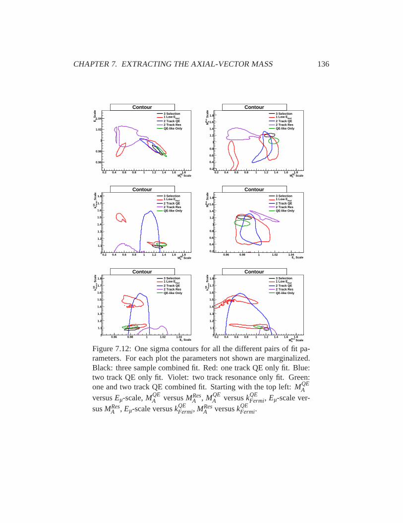
CHAPTER 7. EXTRACTING THE AXIAL-VECTOR MASS 136
ScaleQEAM
0.2 0.4 0.6 0.8 1 1.2 1.4 1.6 1.8
Sca
leµ
E
0.96
0.98
1
1.02
1.04
Contour3 Selection
Had1 Low E2 Track QE2 Track ResQE-like Only
3 SelectionHad1 Low E
2 Track QE2 Track ResQE-like Only
3 SelectionHad1 Low E
2 Track QE2 Track ResQE-like Only
3 SelectionHad1 Low E
2 Track QE2 Track ResQE-like Only
3 SelectionHad1 Low E
2 Track QE2 Track ResQE-like Only
Contour
ScaleQEAM
0.2 0.4 0.6 0.8 1 1.2 1.4 1.6 1.8
Sca
leR
esA
M
0.2
0.4
0.6
0.8
1
1.2
1.4
1.6
1.8
Contour3 Selection
Had1 Low E2 Track QE2 Track ResQE-like Only
3 SelectionHad1 Low E
2 Track QE2 Track ResQE-like Only
3 SelectionHad1 Low E
2 Track QE2 Track ResQE-like Only
3 SelectionHad1 Low E
2 Track QE2 Track ResQE-like Only
3 SelectionHad1 Low E
2 Track QE2 Track ResQE-like Only
Contour
ScaleQEAM
0.2 0.4 0.6 0.8 1 1.2 1.4 1.6 1.8
Sca
leQ
EF
erm
ik
1
1.1
1.2
1.3
1.4
1.5
1.6
1.7
1.8
Contour3 Selection
Had1 Low E2 Track QE2 Track ResQE-like Only
3 SelectionHad1 Low E
2 Track QE2 Track ResQE-like Only
3 SelectionHad1 Low E
2 Track QE2 Track ResQE-like Only
3 SelectionHad1 Low E
2 Track QE2 Track ResQE-like Only
3 SelectionHad1 Low E
2 Track QE2 Track ResQE-like Only
Contour
ScaleµE0.96 0.98 1 1.02 1.04
Sca
leR
esA
M
0.2
0.4
0.6
0.8
1
1.2
1.4
1.6
1.8
Contour3 Selection
Had1 Low E2 Track QE2 Track ResQE-like Only
3 SelectionHad1 Low E
2 Track QE2 Track ResQE-like Only
3 SelectionHad1 Low E
2 Track QE2 Track ResQE-like Only
3 SelectionHad1 Low E
2 Track QE2 Track ResQE-like Only
3 SelectionHad1 Low E
2 Track QE2 Track ResQE-like Only
Contour
ScaleµE0.96 0.98 1 1.02 1.04
Sca
leQ
EF
erm
ik
1
1.1
1.2
1.3
1.4
1.5
1.6
1.7
1.8
Contour3 Selection
Had1 Low E2 Track QE2 Track ResQE-like Only
3 SelectionHad1 Low E
2 Track QE2 Track ResQE-like Only
3 SelectionHad1 Low E
2 Track QE2 Track ResQE-like Only
3 SelectionHad1 Low E
2 Track QE2 Track ResQE-like Only
3 SelectionHad1 Low E
2 Track QE2 Track ResQE-like Only
Contour
ScaleResAM
0.2 0.4 0.6 0.8 1 1.2 1.4 1.6 1.8
Sca
leQ
EF
erm
ik
1
1.1
1.2
1.3
1.4
1.5
1.6
1.7
1.8
Contour3 Selection
Had1 Low E2 Track QE2 Track ResQE-like Only
3 SelectionHad1 Low E
2 Track QE2 Track ResQE-like Only
3 SelectionHad1 Low E
2 Track QE2 Track ResQE-like Only
3 SelectionHad1 Low E
2 Track QE2 Track ResQE-like Only
3 SelectionHad1 Low E
2 Track QE2 Track ResQE-like Only
Contour
Figure 7.12: One sigma contours for all the different pairs of fit pa-rameters. For each plot the parameters not shown are marginalized.Black: three sample combined fit. Red: one track QE only fit. Blue:two track QE only fit. Violet: two track resonance only fit. Green:one and two track QE combined fit. Starting with the top left:MQE
A
versusEµ-scale,MQEA versusMRes
A , MQEA versuskQE
Fermi, Eµ-scale ver-susMRes
A , Eµ-scale versuskQEFermi, MRes
A versuskQEFermi.

CHAPTER 7. EXTRACTING THE AXIAL-VECTOR MASS 137
unused hits selection criteria. Thus any differences between data and MC in the
two track QE sideband are expected to show up in the two track background-like
sub-sample. The parameters used to describe the three sub-sample in this analysis
are sufficient to describe each individual selection, however they are not sufficient
to describe all three sub-samples simultaneously. This supports the hypothesis
that there is one or more unsimulated types of interactions in the data.
There is enough evidence that there are one or more types of unsimulated
interactions getting classified as background interactions to warrant the inclusion
of some kind of background correction function within this analysis. However
there are clearly correlations between the parameters thatcontrol the shape of the
background and the parameters that control the shape of the signal. The ideal
solution is what has already been tried, fit everything simultaneously, however
that no longer seems possible. It appears that a whole new fit procedure is needed.
7.5 New Fit Procedure
Unsurprisingly the tension that exists between the two track background-like sub-
sample and the two QE-like sub-samples is primarily in the parameter that controls
the shape of the background. IndividuallyMResA is sufficient to describe the shape
of the background. Theχ2 for all the individual fits are reasonable given the
number of degrees of freedom,MRESA is only insufficient when trying to use it
to describe the shape of the resonances in all three sub-samples simultaneously.
BecauseMResA is sufficient to describe the shape of the resonances in each selection
individually, but not sufficient to describe all three selections simultaneously, it is
necessary to develop a fit procedure that extracts the data/MC differences in the
resonances events that aren’t being described using theMResA parameter.
7.5.1 Fit Steps
A fit procedure that meets all of the preceding requirements can be constructed
using the following steps:

CHAPTER 7. EXTRACTING THE AXIAL-VECTOR MASS 138
1. Fit: fit only the QE-like selections.
2. Characterize the QE: feed the best fit parameters from the simultaneous fit
of both QE-like selections into the two track resonance selection.
3. Event Subtraction: subtract the predicted true QE eventsfrom the data in
the two track resonance selection.
4. Fit two track resonance: fit the two track resonance selection (with no true
QE events) using theMResA parameter as the only free parameter, every other
parameter is fixed.
5. Background Correction: use the data/MC spectrum from thetwo track res-
onance selection, parameterized using a cubic polynomial,as a correction
to the background of the QE-like selections.
6. Repeat Fit: perform this procedure again until the background correction
function agrees with the background correction function ofthe previous
iteration.
The disadvantage in this fit procedure is the best fit value of theMResA parameter is
essentially meaningless. In effect there are two differentbest fit values forMResA :
One from the simultaneous fit of the QE-like sub-samples, andone from the from
the fit of the two track background-like sub-sample. TheMResA parameter is being
used instead to describe (along with the background correction function) the shape
of what appears to be the resonances plus some other type of interactions that are
not simulated in the MINOS MC.
Even though the value for theMResA parameter is essentially meaningless, the
background correction function provides more confidence inthe measurement for
MQEA . By using the background correction function plus the shapefrom MRes
A , it
is possible to account for correlations between the background shape andMQEA ,
while also accounting for large differences in the background between the data
and model.
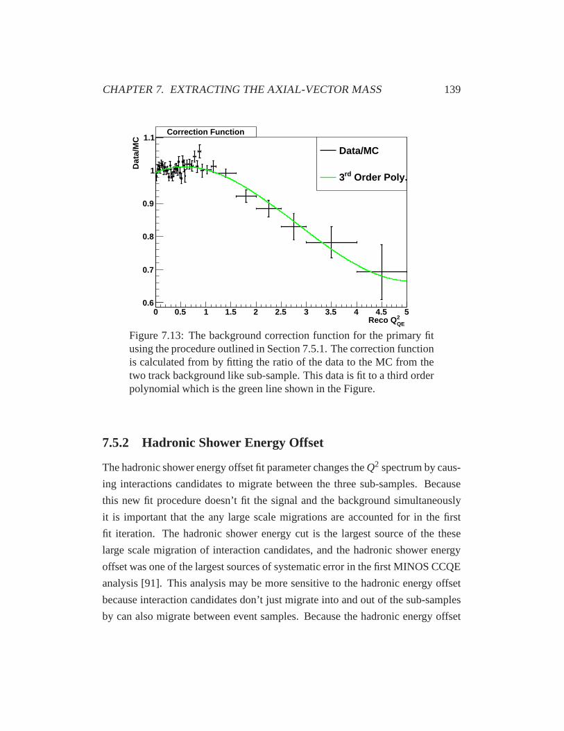
CHAPTER 7. EXTRACTING THE AXIAL-VECTOR MASS 139
QE2 Reco Q
0 0.5 1 1.5 2 2.5 3 3.5 4 4.5 5
Dat
a/M
C
0.6
0.7
0.8
0.9
1
1.1Correction Function
Data/MC
Order Poly.rd3
Figure 7.13: The background correction function for the primary fitusing the procedure outlined in Section 7.5.1. The correction functionis calculated from by fitting the ratio of the data to the MC from thetwo track background like sub-sample. This data is fit to a third orderpolynomial which is the green line shown in the Figure.
7.5.2 Hadronic Shower Energy Offset
The hadronic shower energy offset fit parameter changes theQ2 spectrum by caus-
ing interactions candidates to migrate between the three sub-samples. Because
this new fit procedure doesn’t fit the signal and the background simultaneously
it is important that the any large scale migrations are accounted for in the first
fit iteration. The hadronic shower energy cut is the largest source of the these
large scale migration of interaction candidates, and the hadronic shower energy
offset was one of the largest sources of systematic error in the first MINOS CCQE
analysis [91]. This analysis may be more sensitive to the hadronic energy offset
because interaction candidates don’t just migrate into andout of the sub-samples
by can also migrate between event samples. Because the hadronic energy offset

CHAPTER 7. EXTRACTING THE AXIAL-VECTOR MASS 140
had a large effect on the first MINOS CCQE analysis and this analysis may be
more sensitive to the hadronic energy offset, the hadronic energy offset is fit as an
additional parameter in the new fit procedure.
7.5.3 Fit Results
The fit was performed as outlined above. It was found that the background cor-
rection function from the third iteration agreed with the background correction
function from the second iteration, thus a third fit of the QE-like sub-samples was
not necessary. The best fit results from both the first and second fit iterations are
shown in Table 7.4. TheQ2QE. distributions for the QE-like sub-samples are shown
in Figure 7.14 and the background correction function is shown in Figure 7.13.
Parameter 1st Iteration 2st Iteration
MQEA (GeV) 1.312±0.033 1.315±0.034
Eµ-scale 0.985±0.003 0.986±0.003Ehad-offset 0.0381±0.035 0.0381±0.035MRES
A (GeV) 1.283±0.057 1.256±0.057kQE
Fermi-scale 1.124±0.009 1.120±0.009χ2/ndf 1.201 1.091
Table 7.4: Best fit values for the baseline first and second fit iterationusing the procedure outlined in Section 7.5.1. No further iterationswere necessary because there was very little change in the backgroundcorrection function. The errors shown are theHESSE errors from theMINUIT software package.
There is very little change in theMQEA parameter from the first iteration to
the second iteration. While there is a larger (though not statistically significant)
change in theMRESA parameter. This gives confidence that theMQE
A parameter is
modeling the behavior of the true quasi-elastic interactions within the sub-samples
and not instead accounting for potential model errors within the resonance model.
Furthermore theχ2 is reduced from the first to the second iteration, this indicates

CHAPTER 7. EXTRACTING THE AXIAL-VECTOR MASS 141
that the background correction function that is defined by the background like
sub-sample is increasing the goodness of fit in the QE-like sub-sample.
)2 (GeV2Reco Q0 0.2 0.4 0.6 0.8 1 1.2
Eve
nts/
1e20
PO
T
0
5
10
15
20
25
30
35
40
45
310× One Track QE-Like
Data
Best Fit MC
Nominal MC
True QE MC
One Track QE-Like
)2 (GeV2Reco Q0 0.2 0.4 0.6 0.8 1 1.2
Dat
a/M
C
0.7
0.8
0.9
1
1.1
1.2
One Track QE-Like
Nominal MC
Best Fit MC
One Track QE-Like
)2 (GeV2Reco Q0 0.5 1 1.5 2 2.5 3
Eve
nts/
1e20
PO
T
0
0.5
1
1.5
2
2.5
3310× Two Track QE-Like
Data
Best Fit MC
Nominal MC
True QE MC
Two Track QE-Like
)2 (GeV2Reco Q0 0.5 1 1.5 2 2.5 3
Dat
a/M
C
0.7
0.8
0.9
1
1.1
1.2
Two Track QE-Like
Nominal MC
Best Fit MC
Two Track QE-Like
Figure 7.14: Best fitQ2QE distributions for the fit to data using the pro-
cedure outlined in Section 7.5.1. Top: One track QE-like selection.Bottom: Two track QE-like selection. Red: Best fitQ2
QE distribution.Blue: NominalQ2
QE distribution. Black: Best fitQ2QE distribution of
the true QE composition of the sub-sample. Right: Data/MC ratiobinned using the same binning as the fit.
7.5.4 Systematic Error Contribution
Many other factors contribute to the systematic uncertainty in the quasi-elastic
axial-vector mass, beyond those that are included directlyin the fit. These addi-
tional factors (outlined below) are calculated by re-performing the fit procedure
outline in Section 7.5.1, only the final fit results (from Table 7.4 are used as the

CHAPTER 7. EXTRACTING THE AXIAL-VECTOR MASS 142
initial seed to the fit. The contribution from these various categories are shown in
Table 7.5.
Sub-sample Selection Criteria
This set of systematic shifts consist of changes to the selection criteria that is
used to define the various sub-samples used in this analysis.Changing any of
these parameters causes interaction candidates to migratebetween the defined
sub-samples, or potentially out of one of the defined sub-samples and into a the
sub-sample of interaction candidates that passed the preselection cuts but were
not sorted into one of the defined sub-samples. The quadraticsum of all of the
systematic shift is+0.100−0.183.
100 150 200 250 300 350 400
-Sca
leQ
EA
M
1.1
1.2
1.3
1.4
1.5
Cut Value Systematic (in MeV)HadE Cut Value Systematic (in MeV)HadE
100 150 200 250 300 350 400
-Sca
leµ
E
0.97
0.975
0.98
0.985
0.99
0.995
1
1.005
Cut Value Systematic (in MeV)HadE Cut Value Systematic (in MeV)HadE
100 150 200 250 300 350 400
-Sca
leR
esA
M
0.85
0.9
0.95
1
1.05
1.1
1.15 Cut Value Systematic (in MeV)HadE Cut Value Systematic (in MeV)HadE
100 150 200 250 300 350 400
QE
Fer
mi
k
1.11
1.12
1.13
1.14
1.15
1.16
Cut Value Systematic (in MeV)HadE Cut Value Systematic (in MeV)HadE
Figure 7.15: Best fit values (along with theHESSE) errors for differ-ent definitions of the low hadronic energy sub-sample.
• Low Hadronic Energy Selection Criteria: the low hadronic energy sub-
sample is defined as: all of the preselected interaction candidate with recon-
structed hadronic shower energy less than 250 MeV. Shown in Figure 7.15

CHAPTER 7. EXTRACTING THE AXIAL-VECTOR MASS 143
20 25 27 29 30 31 33 35 40
-Sca
leQ
EA
M
1.2
1.25
1.3
1.35
1.4
Shift Systematic (in degrees)pθ∆ Shift Systematic (in degrees)pθ∆
20 25 27 29 30 31 33 35 40
-Sca
leµ
E
0.978
0.98
0.982
0.984
0.986
0.988
0.99
0.992
Shift Systematic (in degrees)pθ∆ Shift Systematic (in degrees)pθ∆
20 25 27 29 30 31 33 35 40
-Sca
leR
esA
M
1.061.08
1.11.121.141.161.18
1.21.221.241.26
Shift Systematic (in degrees)pθ∆ Shift Systematic (in degrees)pθ∆
20 25 27 29 30 31 33 35 40Q
EF
erm
ik
1.1
1.105
1.11
1.115
1.12
1.125
1.13
1.1351.14
Shift Systematic (in degrees)pθ∆ Shift Systematic (in degrees)pθ∆
Figure 7.16: Best fit values (along with theHESSE errors) for differ-ent definitions of the∆θp dividing line between the two track QE-likeand two track background like sub-samples.
are distributions of possible alternative definitions to the low hadronic en-
ergy selection criteria. A previous study of kinematic resolution in MI-
NOS showed that the appropriate (though conservative) value to express
a ’1σ’ change in the definition of the low hadronic energy sub-sampel is
±100 MeV. This systematic one of the largest single contributions to the
uncertainty on the quasi-elastic axial-vector mass.
• ∆θp Selection: this selection variable in part defines the border between
the two track QE-like sub-sample and the two track background like sub-
sample. This definition was chosen to select the most low∆θp ‘bump’ of
true QE interactions shown in Figure 7.16, while also optimizing the purity
of the two track QE like subsample. This somewhat arbitrary choice of
selection criteria is allowed to vary along the downward slope of this true
QE bump.±5◦ defines the ‘1σ’ change in this systematic.
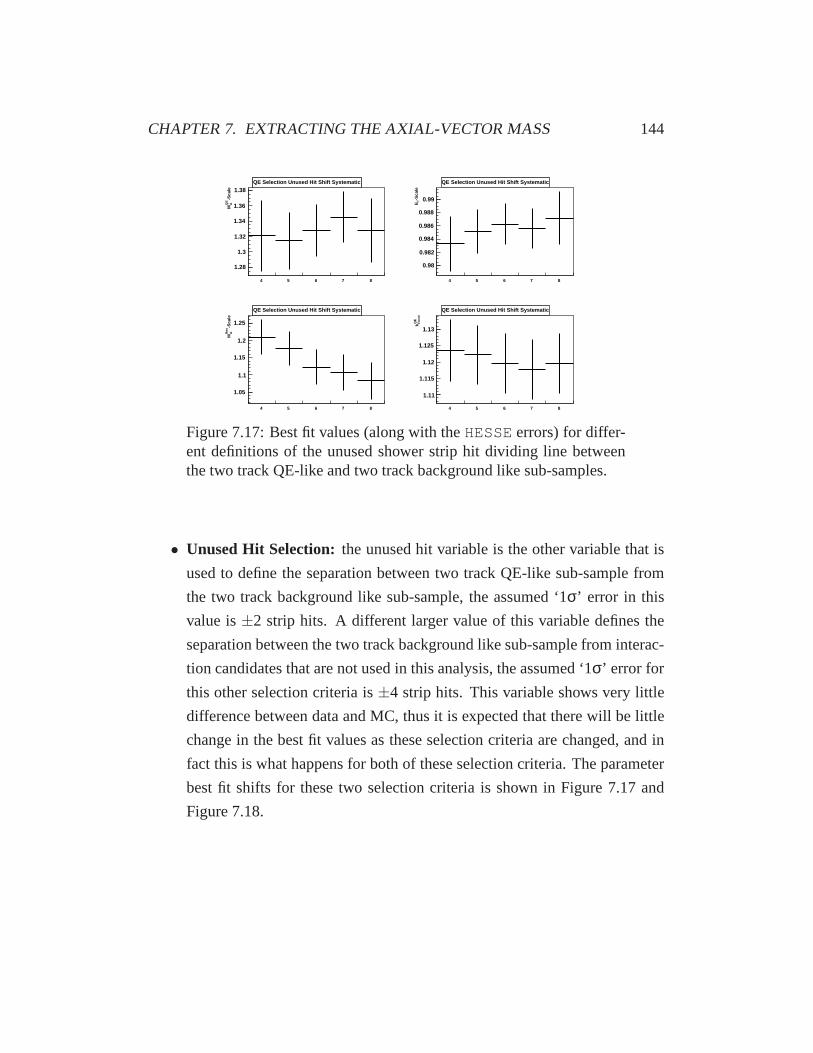
CHAPTER 7. EXTRACTING THE AXIAL-VECTOR MASS 144
4 5 6 7 8
-Sca
leQ
EA
M
1.28
1.3
1.32
1.34
1.36
1.38QE Selection Unused Hit Shift SystematicQE Selection Unused Hit Shift Systematic
4 5 6 7 8
-Sca
leµ
E
0.98
0.982
0.984
0.986
0.988
0.99
QE Selection Unused Hit Shift SystematicQE Selection Unused Hit Shift Systematic
4 5 6 7 8
-Sca
leR
esA
M
1.05
1.1
1.15
1.2
1.25
QE Selection Unused Hit Shift SystematicQE Selection Unused Hit Shift Systematic
4 5 6 7 8Q
EF
erm
ik
1.11
1.115
1.12
1.125
1.13
QE Selection Unused Hit Shift SystematicQE Selection Unused Hit Shift Systematic
Figure 7.17: Best fit values (along with theHESSE errors) for differ-ent definitions of the unused shower strip hit dividing line betweenthe two track QE-like and two track background like sub-samples.
• Unused Hit Selection: the unused hit variable is the other variable that is
used to define the separation between two track QE-like sub-sample from
the two track background like sub-sample, the assumed ‘1σ’ error in this
value is±2 strip hits. A different larger value of this variable defines the
separation between the two track background like sub-sample from interac-
tion candidates that are not used in this analysis, the assumed ‘1σ’ error for
this other selection criteria is±4 strip hits. This variable shows very little
difference between data and MC, thus it is expected that there will be little
change in the best fit values as these selection criteria are changed, and in
fact this is what happens for both of these selection criteria. The parameter
best fit shifts for these two selection criteria is shown in Figure 7.17 and
Figure 7.18.

CHAPTER 7. EXTRACTING THE AXIAL-VECTOR MASS 145
11 12 13 14 15 16 17
-Sca
leQ
EA
M
1.29
1.3
1.31
1.32
1.33
1.34
1.35
1.36
Res Selection Unused Hit Shift SystematicRes Selection Unused Hit Shift Systematic
11 12 13 14 15 16 17
-Sca
leµ
E
0.983
0.984
0.985
0.986
0.987
0.988
0.989
0.99
Res Selection Unused Hit Shift SystematicRes Selection Unused Hit Shift Systematic
11 12 13 14 15 16 17
-Sca
leR
esA
M
1.06
1.08
1.1
1.12
1.14
1.16
1.18Res Selection Unused Hit Shift SystematicRes Selection Unused Hit Shift Systematic
11 12 13 14 15 16 17Q
EF
erm
ik
1.11
1.115
1.12
1.125
1.13Res Selection Unused Hit Shift SystematicRes Selection Unused Hit Shift Systematic
Figure 7.18: Best fit values (along with theHESSE errors) for differ-ent definitions of the unused shower strip hit dividing line betweenthe two track background like and the sub-sample of interaction can-didates that are not used in this analysis.
Beam Flux Uncertainty
The beam flux is applied a little differently in this analysisthen in the MINOS
oscillation analysis for which the procedure was originally developed. Hadron
production weights are applied to the primary fit (Table 7.4)then systematic shifts
are considered for all of the beam optics nuance parameters (excepting the POT
error which is only a normalization error and irrelevant fora shape only fit). While
parameters very similar to the detector parameters are already applied within the
primary fit. Furthermore additional systematics are considered where the hadron
production parameters are reset to there nominal values. Anadditional shift of
±5 cm shift in thezposition of the target is also considered. This final systematic
shift does not express an uncertainty of±5 cm to the actually target position but
is instead a stand in for some other unknown effect that couldbe causing the peak
of the entire neutrino energy distribution to move. The quadratic sum of the beam
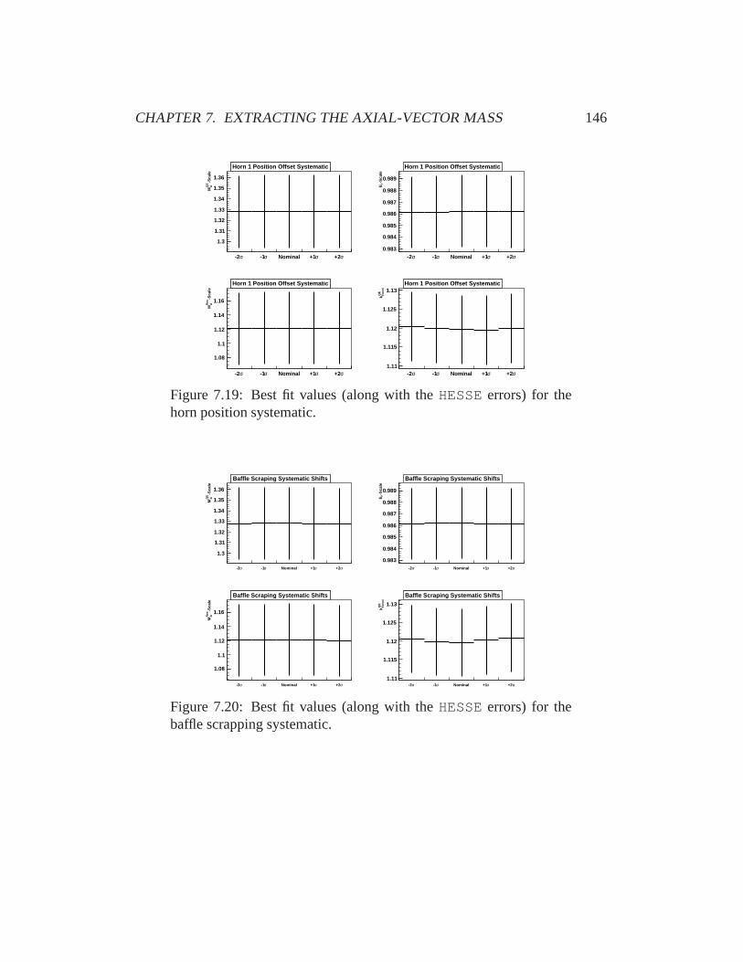
CHAPTER 7. EXTRACTING THE AXIAL-VECTOR MASS 146
σ-2 σ-1 Nominal σ+1 σ+2
-Sca
leQ
EA
M
1.3
1.31
1.32
1.33
1.34
1.35
1.36
Horn 1 Position Offset SystematicHorn 1 Position Offset Systematic
σ-2 σ-1 Nominal σ+1 σ+2
-Sca
leµ
E
0.983
0.984
0.985
0.986
0.987
0.988
0.989
Horn 1 Position Offset SystematicHorn 1 Position Offset Systematic
σ-2 σ-1 Nominal σ+1 σ+2
-Sca
leR
esA
M
1.08
1.1
1.12
1.14
1.16
Horn 1 Position Offset SystematicHorn 1 Position Offset Systematic
σ-2 σ-1 Nominal σ+1 σ+2Q
EF
erm
ik
1.11
1.115
1.12
1.125
1.13Horn 1 Position Offset SystematicHorn 1 Position Offset Systematic
Figure 7.19: Best fit values (along with theHESSE errors) for thehorn position systematic.
σ-2 σ-1 Nominal σ+1 σ+2
-Sca
leQ
EA
M
1.3
1.31
1.32
1.33
1.34
1.35
1.36
Baffle Scraping Systematic ShiftsBaffle Scraping Systematic Shifts
σ-2 σ-1 Nominal σ+1 σ+2
-Sca
leµ
E
0.983
0.984
0.985
0.986
0.987
0.988
0.989
Baffle Scraping Systematic ShiftsBaffle Scraping Systematic Shifts
σ-2 σ-1 Nominal σ+1 σ+2
-Sca
leR
esA
M
1.08
1.1
1.12
1.14
1.16
Baffle Scraping Systematic ShiftsBaffle Scraping Systematic Shifts
σ-2 σ-1 Nominal σ+1 σ+2
QE
Fer
mi
k
1.11
1.115
1.12
1.125
1.13
Baffle Scraping Systematic ShiftsBaffle Scraping Systematic Shifts
Figure 7.20: Best fit values (along with theHESSE errors) for thebaffle scrapping systematic.

CHAPTER 7. EXTRACTING THE AXIAL-VECTOR MASS 147
σ-2 σ-1 Nominal σ+1 σ+2
-Sca
leQ
EA
M
1.29
1.31.31
1.32
1.331.34
1.351.36
1.37
Horn Current Calibration SystematicHorn Current Calibration Systematic
σ-2 σ-1 Nominal σ+1 σ+2
-Sca
leµ
E
0.983
0.984
0.985
0.986
0.987
0.988
0.989
0.99Horn Current Calibration SystematicHorn Current Calibration Systematic
σ-2 σ-1 Nominal σ+1 σ+2
-Sca
leR
esA
M
1.06
1.08
1.1
1.12
1.14
1.16
1.18Horn Current Calibration SystematicHorn Current Calibration Systematic
σ-2 σ-1 Nominal σ+1 σ+2
QE
Fer
mi
k
1.105
1.11
1.115
1.12
1.125
1.13
1.135Horn Current Calibration SystematicHorn Current Calibration Systematic
Figure 7.21: Best fit values (along with theHESSE errors) for thehorn current calibration systematic.
σ-2 σ-1 Nominal σ+1 σ+2
-Sca
leQ
EA
M
1.29
1.3
1.31
1.32
1.33
1.34
1.35
1.36
1.37
Horn 1 Current Distribution SystematicHorn 1 Current Distribution Systematic
σ-2 σ-1 Nominal σ+1 σ+2
-Sca
leµ
E
0.983
0.984
0.985
0.986
0.987
0.988
0.989
0.99Horn 1 Current Distribution SystematicHorn 1 Current Distribution Systematic
σ-2 σ-1 Nominal σ+1 σ+2
-Sca
leR
esA
M
1.08
1.1
1.12
1.14
1.16
1.18Horn 1 Current Distribution SystematicHorn 1 Current Distribution Systematic
σ-2 σ-1 Nominal σ+1 σ+2
QE
Fer
mi
k
1.105
1.11
1.115
1.12
1.125
1.13
1.135Horn 1 Current Distribution SystematicHorn 1 Current Distribution Systematic
Figure 7.22: Best fit values (along with theHESSE errors) for thehorn current distribution systematic.

CHAPTER 7. EXTRACTING THE AXIAL-VECTOR MASS 148
flux uncertainty contribution to the quasi-elastic axial-vector mass is+0.020−0.019.
-5cmTargetZ Nominal +5cmTargetZ Tunning
-Sca
leQ
EA
M
1.28
1.3
1.32
1.34
1.36
1.38
Beam SystematicsBeam Systematics
-5cmTargetZ Nominal +5cmTargetZ Tunning
-Sca
leµ
E
0.982
0.983
0.984
0.985
0.986
0.987
0.988
0.989
0.99
0.991Beam SystematicsBeam Systematics
-5cmTargetZ Nominal +5cmTargetZ Tunning
-Sca
leR
esA
M
1.06
1.08
1.1
1.12
1.14
1.16
1.18
1.2
Beam SystematicsBeam Systematics
-5cmTargetZ Nominal +5cmTargetZ Tunning
QE
Fer
mi
k
1.1
1.11
1.12
1.13
1.14
Beam SystematicsBeam Systematics
Figure 7.23: Best fit values (along with theHESSE errors) for thetargetzposition along with hadron production systematics.
DIS Model Uncertainty
DIS interactions contribute∼10% of the number of interaction candidates to the
QE-like sub-samples, and∼25% to the two track background like sub-sample.
Thus the primary way that the DIS model contributes to the measurement of the
MQEA parameter is through the shape of the background correctionfunction. Un-
certainties in the DIS model are addressed by considering±1σ changes to ther i j 2
andr i j 3 parameters of the KNO model of DIS interactions. These parameters in-
crease or decrease the contribution of two pions (r i j 2), and three pions (r i j 3) final
states to theQ2 distributions. The quadratic sum of the DIS model uncertainty
contribution to the QE axial-vector mass is+0.014−0.025.

CHAPTER 7. EXTRACTING THE AXIAL-VECTOR MASS 149
nominal σ+1π2 σ-1π2 σ+1π3 σ-1π3
-Sca
leQ
EA
M
1.28
1.3
1.32
1.34
1.36
1.38Deep Inelastic Scattring ModelDeep Inelastic Scattring Model
nominal σ+1π2 σ-1π2 σ+1π3 σ-1π3
-Sca
leµ
E
0.983
0.984
0.985
0.986
0.987
0.988
0.989
0.99
Deep Inelastic Scattring ModelDeep Inelastic Scattring Model
nominal σ+1π2 σ-1π2 σ+1π3 σ-1π3
-Sca
leR
esA
M
1
1.05
1.1
1.15
1.2
1.25Deep Inelastic Scattring ModelDeep Inelastic Scattring Model
nominal σ+1π2 σ-1π2 σ+1π3 σ-1π3Q
EF
erm
ik
1.105
1.11
1.115
1.12
1.125
1.13
1.135
Deep Inelastic Scattring ModelDeep Inelastic Scattring Model
Figure 7.24: Best fit values (along with theHESSE errors) for the DISmodel systematic.
σ-1 nominal σ+1
-Sca
leQ
EA
M
1.1
1.15
1.2
1.25
1.3
1.35
1.4
1.45Low Q^2 Resonance SuppressionLow Q^2 Resonance Suppression
σ-1 nominal σ+1
-Sca
leµ
E
0.98
0.985
0.99
0.995
1
1.005
Low Q^2 Resonance SuppressionLow Q^2 Resonance Suppression
σ-1 nominal σ+1
-Sca
leR
esA
M
0.981
1.021.041.061.08
1.11.121.14
1.161.18
Low Q^2 Resonance SuppressionLow Q^2 Resonance Suppression
σ-1 nominal σ+1
QE
Fer
mi
k
1.11
1.12
1.13
1.14
1.15
1.16
Low Q^2 Resonance SuppressionLow Q^2 Resonance Suppression
Figure 7.25: Best fit values (along with theHESSE errors) due to thelow Q2 resonance suppression function.
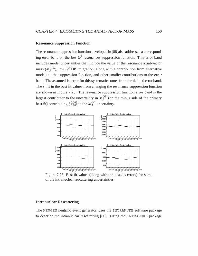
CHAPTER 7. EXTRACTING THE AXIAL-VECTOR MASS 150
Resonance Suppression Function
The resonance suppression function developed in [88]also addressed a correspond-
ing error band on the lowQ2 resonances suppression function. This error band
includes model uncertainties that include the value of the resonance axial-vector
mass (MRESA ), low Q2 DIS migration, along with a contribution from alternative
models to the suppression function, and other smaller contributions to the error
band. The assumed 1σ error for this systematic comes from the defined error band.
The shift in the best fit values from changing the resonance suppression function
are shown in Figure 7.25. The resonance suppression function error band is the
largest contributor to the uncertainty inMQEA (on the minus side of the primary
best fit) contributing+0.066−0.188 to theMQE
A uncertainty.
Nominal
σ
charge exc +1
π
σ
charge exc -1
π
σ elastic +1
π
σ elastic 11
π
σ
inelastic +1
π
σ
inelastic -1
π
σ
absorb +1
π
σ absorb -1
πσ +1π->2π
σ -1π->2π
-Sca
leQ
EA
M
1.28
1.3
1.32
1.34
1.36
Intra Nuke SystematicsIntra Nuke Systematics
Nominal
σ
charge exc +1
π
σ
charge exc -1
π
σ elastic +1
π
σ elastic 11
π
σ
inelastic +1
π
σ
inelastic -1
π
σ
absorb +1
π
σ absorb -1
πσ +1π->2π
σ -1π->2π
-Sca
leµ
E
0.983
0.984
0.985
0.986
0.987
0.988
0.989
0.99Intra Nuke SystematicsIntra Nuke Systematics
Nominal
σ
charge exc +1
π
σ
charge exc -1
π
σ elastic +1
π
σ elastic 11
π
σ
inelastic +1
π
σ
inelastic -1
π
σ
absorb +1
π
σ absorb -1
πσ +1π->2π
σ -1π->2π
-Sca
leR
esA
M
1.06
1.08
1.1
1.12
1.14
1.16
1.18
Intra Nuke SystematicsIntra Nuke Systematics
Nominal
σ
charge exc +1
π
σ
charge exc -1
π
σ elastic +1
π
σ elastic 11
π
σ
inelastic +1
π
σ
inelastic -1
π
σ
absorb +1
π
σ absorb -1
πσ +1π->2π
σ -1π->2π
QE
Fer
mi
k
1.11
1.115
1.12
1.125
1.13
Intra Nuke SystematicsIntra Nuke Systematics
Figure 7.26: Best fit values (along with theHESSE errors) for someof the intranuclear rescattering uncertainties.
Intranuclear Rescattering
TheNEUGEN neutrino event generator, uses theINTRANUKE software package
to describe the intranuclear rescattering [80]. Using theINTRANUKE package
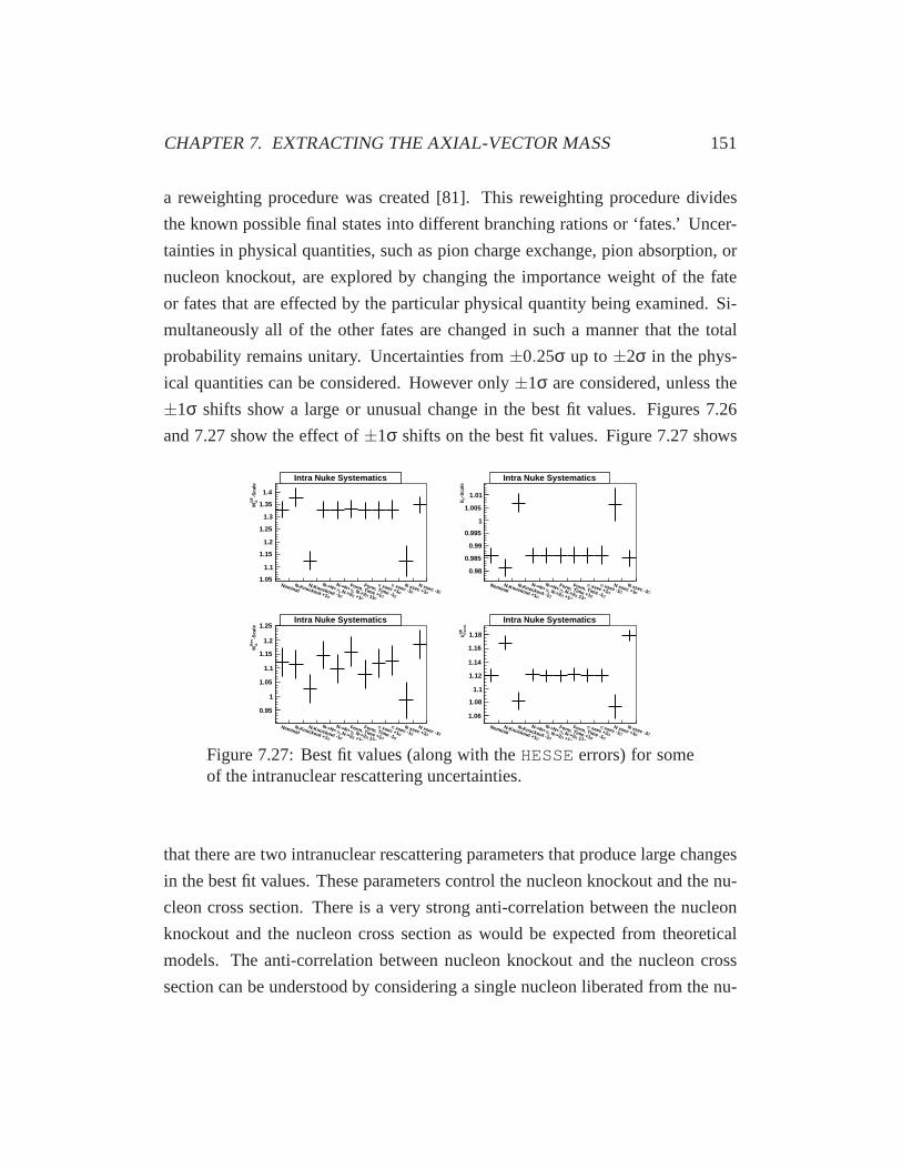
CHAPTER 7. EXTRACTING THE AXIAL-VECTOR MASS 151
a reweighting procedure was created [81]. This reweightingprocedure divides
the known possible final states into different branching rations or ‘fates.’ Uncer-
tainties in physical quantities, such as pion charge exchange, pion absorption, or
nucleon knockout, are explored by changing the importance weight of the fate
or fates that are effected by the particular physical quantity being examined. Si-
multaneously all of the other fates are changed in such a manner that the total
probability remains unitary. Uncertainties from±0.25σ up to±2σ in the phys-
ical quantities can be considered. However only±1σ are considered, unless the
±1σ shifts show a large or unusual change in the best fit values. Figures 7.26
and 7.27 show the effect of±1σ shifts on the best fit values. Figure 7.27 shows
Nominal
σ
N-Knockout +1 σ
N-Knockout -1σ +1π
, N->2π
N->N+
σ 11π, N->2
πN->N+
σ
Form. Time +1 σ
Form. Time -1 σ xsec +1
πσ
xsec -1π
σN xsec +1 σ
N xsec -1
-Sca
leQ
EA
M
1.05
1.1
1.15
1.2
1.25
1.3
1.35
1.4
Intra Nuke SystematicsIntra Nuke Systematics
Nominal
σ
N-Knockout +1 σ
N-Knockout -1σ +1π
, N->2π
N->N+
σ 11π, N->2
πN->N+
σ
Form. Time +1 σ
Form. Time -1 σ xsec +1
πσ
xsec -1π
σN xsec +1 σ
N xsec -1
-Sca
leµ
E
0.98
0.985
0.99
0.995
1
1.005
1.01
Intra Nuke SystematicsIntra Nuke Systematics
Nominal
σ
N-Knockout +1 σ
N-Knockout -1σ +1π
, N->2π
N->N+
σ 11π, N->2
πN->N+
σ
Form. Time +1 σ
Form. Time -1 σ xsec +1
πσ
xsec -1π
σN xsec +1 σ
N xsec -1
-Sca
leR
esA
M
0.95
1
1.05
1.1
1.15
1.2
1.25Intra Nuke SystematicsIntra Nuke Systematics
Nominal
σ
N-Knockout +1 σ
N-Knockout -1σ +1π
, N->2π
N->N+
σ 11π, N->2
πN->N+
σ
Form. Time +1 σ
Form. Time -1 σ xsec +1
πσ
xsec -1π
σN xsec +1 σ
N xsec -1
QE
Fer
mi
k
1.06
1.08
1.1
1.12
1.14
1.16
1.18
Intra Nuke SystematicsIntra Nuke Systematics
Figure 7.27: Best fit values (along with theHESSE errors) for someof the intranuclear rescattering uncertainties.
that there are two intranuclear rescattering parameters that produce large changes
in the best fit values. These parameters control the nucleon knockout and the nu-
cleon cross section. There is a very strong anti-correlation between the nucleon
knockout and the nucleon cross section as would be expected from theoretical
models. The anti-correlation between nucleon knockout andthe nucleon cross
section can be understood by considering a single nucleon liberated from the nu-

CHAPTER 7. EXTRACTING THE AXIAL-VECTOR MASS 152
cleus as a result of a neutrino scattering interaction. Whena nucleon is liberated
from the nucleus, the nucleon recoils from the parent collision with significant
additional momentum. As the recoil nucleon scatters away from the parent col-
lision the recoil nucleon may re-scatter off of other nucleons within the nucleus.
At the lower momentum transfers (< 2 GeV) selected in this analysis, every sec-
ondary nucleon-nucleon collision divides the originally imparted between both of
the nucleons. Increasing the nucleon cross section will increase the number of
these nucleon-nucleon interactions. If the original recoil nucleon losses enough
momentum due to these nucleon-nucleon interactions, the original recoil nucleon,
and likely all of the subsequent nucleons will not leave the nucleus. Thus in-
creasing the nucleon cross section will reduce the number ofnucleons in the final
state. Figure 7.28 demonstrates this correlation between nucleon knockout and
the nucleon cross section.
Further examination of Figure 7.28 also reveals that the lowhadronic shower
energy sub-sample is more sensitive to the effect of these intranuclear rescattering
systematics, than the two track QE-like sub-sample. The lowhadronic shower en-
ergy sub-sample shows∼5% change in theQ2QE distribution while the two track
QE-like sample shows an∼2% change in theQ2QE distribution (except for the
lowestQ2QE bin). Because the low hadronic shower energy sub-sample is sensi-
tive to these parameters, it is possible to further constrain these parameters, this
is done by including these intranuclear rescattering parameters directly in the fit.
However this is impossible due to limitations in theINTRANUKE reweighting
system.INTRANUKE’s reweigting system is configured to conserve probability
between the final state branching ratios, if twoINTRANUKE reweight parame-
ters are applied simultaneously probability would not be conserved between the
final state branching ratios. The alternative to including the parameters directly
in the fit is to scan alongχ2 for different values of theseINTRANUKE systemat-
ics. From this scan of theQ2 distribution the defined ‘±1σ’ uncertainty due to
the nucleon knockout and nucleon cross section will be the fractional 1σ change
that results in a∆χ2 of 1 from the minimumχ2. Theseχ2 scans are shown in

CHAPTER 7. EXTRACTING THE AXIAL-VECTOR MASS 153
QE2Reco Q
0 0.2 0.4 0.6 0.8 1 1.2
data
/MC
0.7
0.8
0.9
1
1.1
1.2
Nominal MC+1$sigma N Knck Out-1$sigma N Knck Out+1$sigma N X-section-1$sigma N X-section
One Track QE-Like
QE2Reco Q
0 0.2 0.4 0.6 0.8 1 1.2
Nom
inal
MC
/Adj
uste
d M
C
0.90.920.940.960.98
11.021.041.061.08
1.1One Track QE-Like
QE2Reco Q
0 0.5 1 1.5 2 2.5 3
data
/MC
0.7
0.8
0.9
1
1.1
1.2
Nominal MC+1$sigma N Knck Out-1$sigma N Knck Out+1$sigma N X-section-1$sigma N X-section
Two Track QE-Like
QE2Reco Q
0 0.5 1 1.5 2 2.5 3
Nom
inal
MC
/Adj
uste
d M
C
0.90.920.940.960.98
11.021.041.061.08
1.1Two Track QE-Like
Figure 7.28: Left: the ratio of data to MC for the nominal MC alongwith the±1σ shifts to the nucleon knockout and nucleon cross sec-tion intranuclear rescattering systematics applied to thenominal MC.Right: the ratio of the nominal MC to the±1σ nucleon knockoutand nucleon cross section intranuclear rescattering systematics ap-plied to the nominal MC. Above: the low hadronic energy QE-likesub-sample. Below: the two track QE-like sub-sample.
Figures 7.29 and 7.30. The uncertainty due to the model of intranuclear rescatter-
ing contributes+0.016−0.023 to theMQE
A uncertainty. Figures 7.29 and 7.30 both show
that the data prefers the nominal MC over any change in the nucleon knockout or
nucleon cross section parameters, these Figures also show that a change in these
parameters of±0.25σ produce a∆χ2 of ∼2. Thus±0.25σ is used as a conserva-
tive estimate of the uncertainty in the neutrino cross section fit parameters due to
the uncertainty in the nucleon knockout and nucleon cross section INTRANUKE
parameters. Figure 7.31 reproduces Figure 7.27 with the newdefinition of 1σINTRANUKE changes.
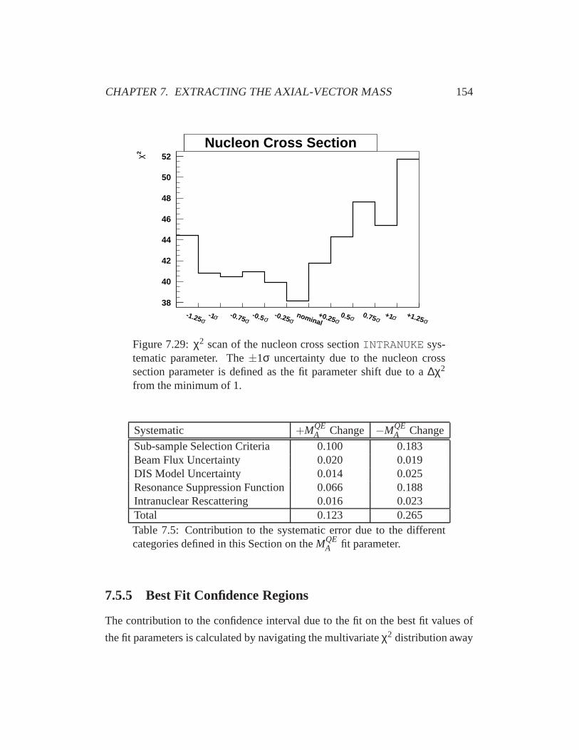
CHAPTER 7. EXTRACTING THE AXIAL-VECTOR MASS 154
σ-1.25 σ-1
σ-0.75 σ-0.5 σ
-0.25 nominal σ+0.25 σ0.5 σ
0.75 σ+1σ
+1.25
2 χ
38
40
42
44
46
48
50
52Nucleon Cross SectionNucleon Cross Section
Figure 7.29:χ2 scan of the nucleon cross sectionINTRANUKE sys-tematic parameter. The±1σ uncertainty due to the nucleon crosssection parameter is defined as the fit parameter shift due to a∆χ2
from the minimum of 1.
Systematic +MQEA Change −MQE
A Change
Sub-sample Selection Criteria 0.100 0.183Beam Flux Uncertainty 0.020 0.019DIS Model Uncertainty 0.014 0.025Resonance Suppression Function 0.066 0.188Intranuclear Rescattering 0.016 0.023Total 0.123 0.265Table 7.5: Contribution to the systematic error due to the differentcategories defined in this Section on theMQE
A fit parameter.
7.5.5 Best Fit Confidence Regions
The contribution to the confidence interval due to the fit on the best fit values of
the fit parameters is calculated by navigating the multivariateχ2 distribution away
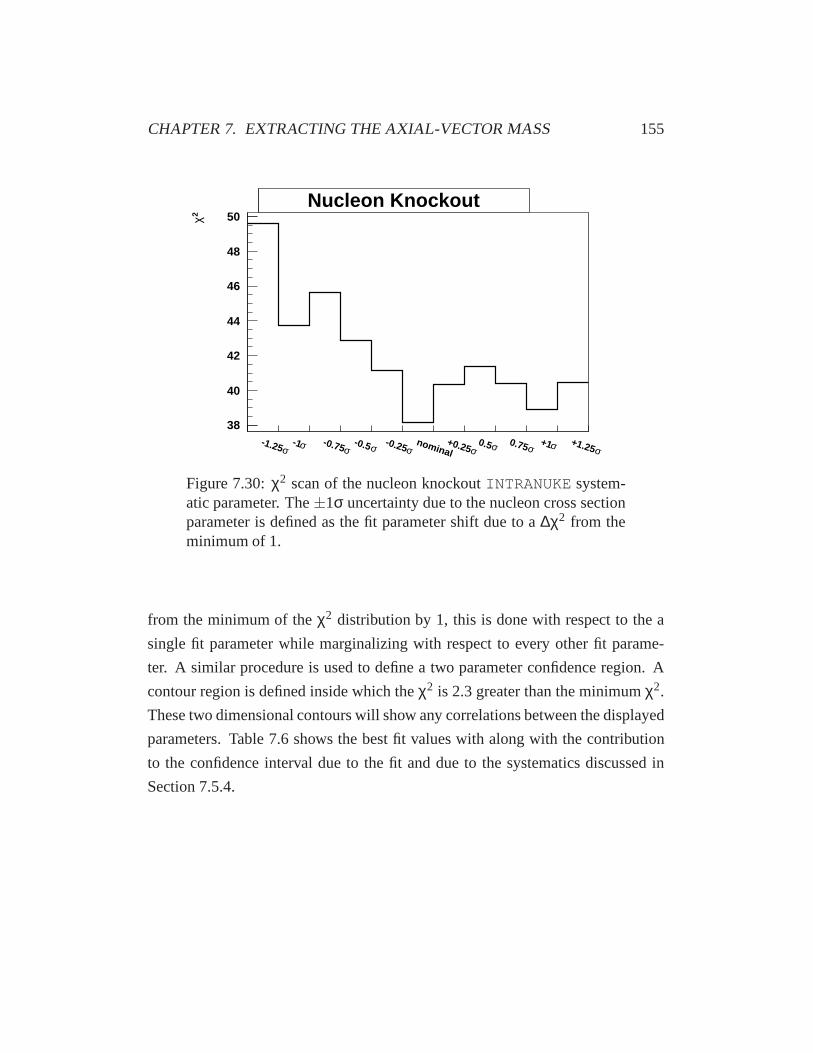
CHAPTER 7. EXTRACTING THE AXIAL-VECTOR MASS 155
σ-1.25 σ-1
σ-0.75 σ-0.5 σ
-0.25 nominal σ+0.25 σ0.5 σ
0.75 σ+1σ
+1.25
2 χ
38
40
42
44
46
48
50Nucleon KnockoutNucleon Knockout
Figure 7.30:χ2 scan of the nucleon knockoutINTRANUKE system-atic parameter. The±1σ uncertainty due to the nucleon cross sectionparameter is defined as the fit parameter shift due to a∆χ2 from theminimum of 1.
from the minimum of theχ2 distribution by 1, this is done with respect to the a
single fit parameter while marginalizing with respect to every other fit parame-
ter. A similar procedure is used to define a two parameter confidence region. A
contour region is defined inside which theχ2 is 2.3 greater than the minimumχ2.
These two dimensional contours will show any correlations between the displayed
parameters. Table 7.6 shows the best fit values with along with the contribution
to the confidence interval due to the fit and due to the systematics discussed in
Section 7.5.4.

CHAPTER 7. EXTRACTING THE AXIAL-VECTOR MASS 156
Nominal σ
N-Knck +1 σN-Knck -1
σ -1π, N->2
πN->N+
σ +1π, N->2
πN->N+
σ
Form. Time +1 σ
Form. Time -1 σ xsec +1
πσ
xsec -1π
σN xsec +1 σ
N xsec -1
-Sca
leQ
EA
M
1.281.29
1.3
1.311.321.331.341.351.361.37
Intra Nuke SystematicsIntra Nuke Systematics
Nominal σ
N-Knck +1 σN-Knck -1
σ -1π, N->2
πN->N+
σ +1π, N->2
πN->N+
σ
Form. Time +1 σ
Form. Time -1 σ xsec +1
πσ
xsec -1π
σN xsec +1 σ
N xsec -1
-Sca
leµ
E
0.983
0.984
0.985
0.986
0.987
0.988
0.989
0.99
Intra Nuke SystematicsIntra Nuke Systematics
Nominal σ
N-Knck +1 σN-Knck -1
σ -1π, N->2
πN->N+
σ +1π, N->2
πN->N+
σ
Form. Time +1 σ
Form. Time -1 σ xsec +1
πσ
xsec -1π
σN xsec +1 σ
N xsec -1
-Sca
leR
esA
M
1.021.041.061.08
1.11.121.141.161.18
1.2
Intra Nuke SystematicsIntra Nuke Systematics
Nominal σ
N-Knck +1 σN-Knck -1
σ -1π, N->2
πN->N+
σ +1π, N->2
πN->N+
σ
Form. Time +1 σ
Form. Time -1 σ xsec +1
πσ
xsec -1π
σN xsec +1 σ
N xsec -1
QE
Fer
mi
k
1.09
1.1
1.11
1.12
1.13
1.14
Intra Nuke SystematicsIntra Nuke Systematics
Figure 7.31: Best fit values (along with theHESSE errors) for someof the intranuclear rescattering uncertainties.
Parameter Best Fit Value Fit Error Systematic Error
MQEA (GeV) 1.315 +0.037
−0.038+0.123−0.265
Eµ-Scale 0.986 +0.004−0.004
+0.022−0.008
MRESA (GeV) 1.256 +0.057
−0.057+0.122−0.221
kQEFermi-Scale 1.120 +0.009
−0.009+0.054−0.028
EHad-Offset (GeV) 0.038 +0.035−0.035
+0.000−0.004
Table 7.6: Best fit values for the along with contributions tothe uncer-tainty due to the fit and the systematics considered in Section 7.5.4.
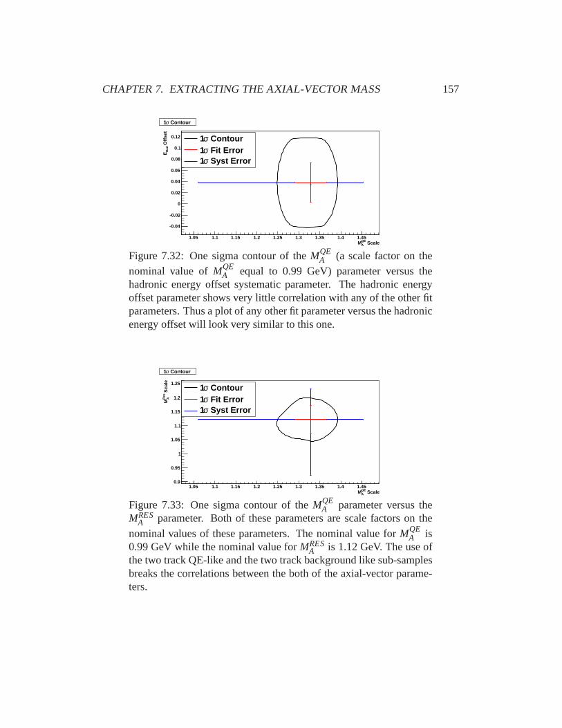
CHAPTER 7. EXTRACTING THE AXIAL-VECTOR MASS 157
ScaleQEA M
1.05 1.1 1.15 1.2 1.25 1.3 1.35 1.4 1.45
Offs
etH
ad E
-0.04
-0.02
0
0.02
0.04
0.06
0.08
0.1
0.12 Contourσ1 Fit Errorσ1 Syst Errorσ1
Contourσ1
Figure 7.32: One sigma contour of theMQEA (a scale factor on the
nominal value ofMQEA equal to 0.99 GeV) parameter versus the
hadronic energy offset systematic parameter. The hadronicenergyoffset parameter shows very little correlation with any of the other fitparameters. Thus a plot of any other fit parameter versus the hadronicenergy offset will look very similar to this one.
ScaleQEA M
1.05 1.1 1.15 1.2 1.25 1.3 1.35 1.4 1.45
Sca
leR
esA
M
0.9
0.95
1
1.05
1.1
1.15
1.2
1.25 Contourσ1 Fit Errorσ1 Syst Errorσ1
Contourσ1
Figure 7.33: One sigma contour of theMQEA parameter versus the
MRESA parameter. Both of these parameters are scale factors on the
nominal values of these parameters. The nominal value forMQEA is
0.99 GeV while the nominal value forMRESA is 1.12 GeV. The use of
the two track QE-like and the two track background like sub-samplesbreaks the correlations between the both of the axial-vector parame-ters.

CHAPTER 7. EXTRACTING THE AXIAL-VECTOR MASS 158
ScaleQEA M
1.05 1.1 1.15 1.2 1.25 1.3 1.35 1.4 1.45
QE
Fer
mi
k
1.09
1.1
1.11
1.12
1.13
1.14
1.15
1.16
1.17
1.18 Contourσ1 Fit Errorσ1 Syst Errorσ1
Contourσ1
Figure 7.34: One sigma contour of theMQEA (a scale factor on the
nominal value ofMQEA equal to 0.99 GeV) parameter versus thekQE
Fermiparameter. The tension between the low hadronic energy offset sub-sample and the two track QE-like sub-sample largely breaks the cor-relation between these parameters. There is still some correlation inthe lower allowed region of the quasi-elasti axial-vector mass param-eter.
ScaleQEA M
1.05 1.1 1.15 1.2 1.25 1.3 1.35 1.4 1.45
Sca
leµ
E
0.98
0.985
0.99
0.995
1
1.005
1.01 Contourσ1 Fit Errorσ1 Syst Errorσ1
Contourσ1
Figure 7.35: One sigma contour of theMQEA (a scale factor on the
nominal value ofMQEA equal to 0.99 GeV) versus theEµ-scale system-
atic parameter. There is a strong correlation between theseparametersdue to the muon energy dependence ofQ2
QE.

CHAPTER 7. EXTRACTING THE AXIAL-VECTOR MASS 159
7.6 Conclusion
Using a simultaneous fit of two statistically independent quasi-elastic dominated
sub-samples of the MINOSνµ-CC event sample, the quasi-elastic axial-vector
mass is measured to be 1.315+0.037−0.038(fit)+0.123
−0.265(syst.) (GeV). Two sub-samples are
used to measureMQEA and are composed primarily of quasi-elastic interactions,
while a third sub-sample which is composed of primarily resonance interactions
is used to constrain the behavior of the background. This measurement is domi-
nated by systematic uncertainties of which the largest uncertainties are due to the
description of the resonances background and the definitionof the low hadronic
energy sub-sample.
Chapter 8
Interpreting the Results
The quasi-elastic axial-vector mass (MQEA ) has been measured to be
1.315+0.037−0.038(fit)+0.123
−0.265(syst.) (GeV) by using a fit to the shape of theQ2QE distri-
bution. This fit was performed simultaneously on two statistically independent
sub-samples of theνµ-CC sample. A third sub-sample was used to constrain the
non-QE background contained within the QE-like sub-samples. This measure-
ment constitutes the first high-statistics measurement ofνµ-CC QE scattering off
of iron.
This value ofMQEA is ∼30% larger than the global mean (circa 2001) of
1.026± 0.021. Furthermore this measurement is dominated by systematic un-
certainties of which the largest contributions come from the definition of the low
hadronic energy sub-sample and the model of the non-QE background.
8.1 Nuclear Effects
There are two indications of the presence of correlations between nucleons within
the nucleus. These are an additional low momentum nucleon (lower momentum
than the recoil nucleon) that recoils in the opposite direction in the zero momen-
tum frame and a transverse enhancement of the neutrinoQ2 differential cross sec-
tion. The transverse enhancement of the neutrinoQ2 differential cross section
160
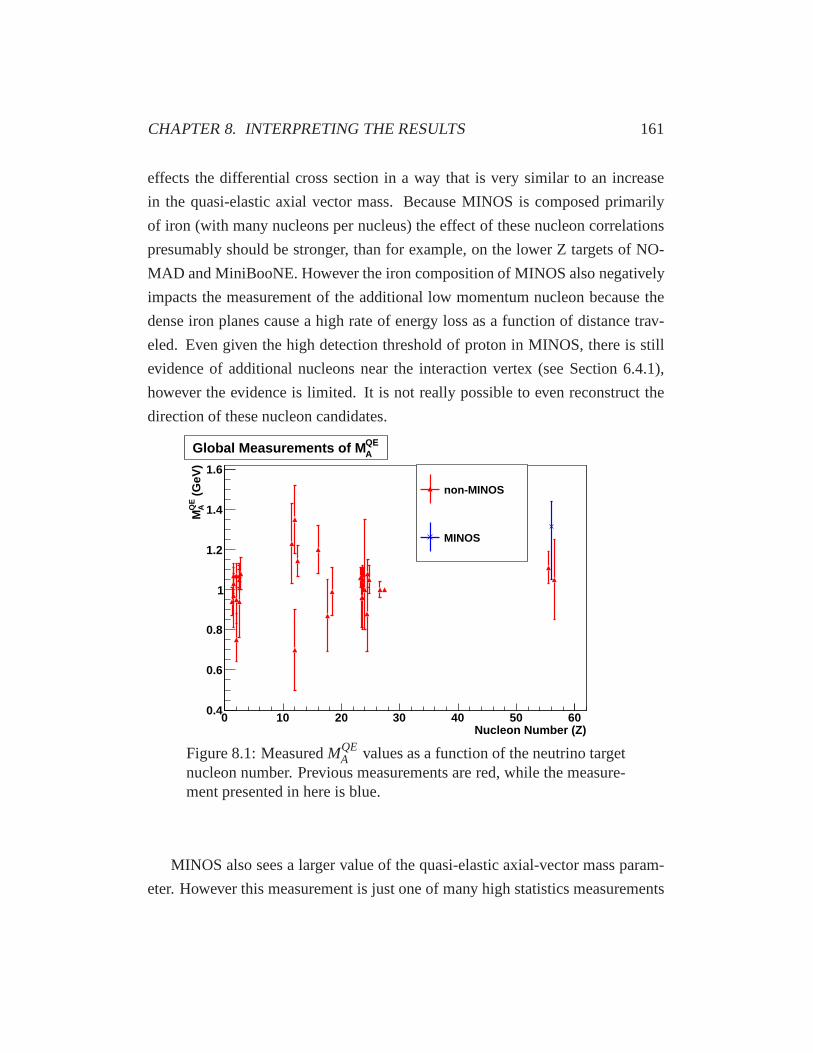
CHAPTER 8. INTERPRETING THE RESULTS 161
effects the differential cross section in a way that is very similar to an increase
in the quasi-elastic axial vector mass. Because MINOS is composed primarily
of iron (with many nucleons per nucleus) the effect of these nucleon correlations
presumably should be stronger, than for example, on the lower Z targets of NO-
MAD and MiniBooNE. However the iron composition of MINOS also negatively
impacts the measurement of the additional low momentum nucleon because the
dense iron planes cause a high rate of energy loss as a function of distance trav-
eled. Even given the high detection threshold of proton in MINOS, there is still
evidence of additional nucleons near the interaction vertex (see Section 6.4.1),
however the evidence is limited. It is not really possible toeven reconstruct the
direction of these nucleon candidates.
Nucleon Number (Z)0 10 20 30 40 50 60
(G
eV)
QE
AM
0.4
0.6
0.8
1
1.2
1.4
1.6
non-MINOS
MINOS
QEAGlobal Measurements of M
Figure 8.1: MeasuredMQEA values as a function of the neutrino target
nucleon number. Previous measurements are red, while the measure-ment presented in here is blue.
MINOS also sees a larger value of the quasi-elastic axial-vector mass param-
eter. However this measurement is just one of many high statistics measurements

CHAPTER 8. INTERPRETING THE RESULTS 162
(low neutrino energy) measurements ofMQEA . What makes MINOS unique is the
iron target. If there is a nucleon number (Z) dependence to the MQEA values, high
Z targets are crucial to discovering it. Figure 8.1 shows theglobal measurements,
from Table 3.1 ofMQEA as a function of the neutrino target Z1 compared to the
measurement ofMQEA measured here. Figure 8.1 shows that there may be a slight
upward trend at higher Z, though this trend is far from conclusive. More measure-
ments with greater precision are needed to identify this potential trend.
8.2 Analysis Improvements
This analysis is systematics limited. Improving this measurement requires im-
proving on the systematic uncertainties. The two systematics that contribute the
largest uncertainties to theMQEA measurement are the definition of the low hadronic
energy sub-sample and the correction to the lowQ2 resonance interactions. Re-
ducing the low hadronic energy systematic requires re-examining the selection
criteria used, while reducing the lowQ2 resonance correction systematic requires
a better understanding of the non-QE background.
8.2.1 Selection Criteria Systematic
At the generator level the distinction between quasi-elastic, resonance, and DIS
scattering can be considered to be a division based on the energy of the hadronic
final state. Quasi-elastic interactions have the lowest final state hadron energy of
these three types of interactions. Originally the low hadronic energy sub-sample
was conceived as an inclusive quasi-elastic sub-sample. Further examination of
the unselected interaction candidates revealed that it waspossible to select addi-
tional quasi-elastics by looking for proton ‘tracks’ giving the two track QE-like
1Some of the measurements ofMQEA used a composite of different materials, for these measure-
ments an average Z was calculated. Several of the measurements list Freon as the target material.Freon is a Dupont brand name for many similar refrigerants, when Freon is listed, CCl2F2 isassumed.

CHAPTER 8. INTERPRETING THE RESULTS 163
sub-sample. This two track QE-like sample was explicitly defined as not low
hadronic shower energy (EHad > 250 MeV). There remains a ‘third’ QE-like sam-
ple with moderateQ2 values between 0.5 GeV2 and 1.5 GeV2 that is not used in
the analysis presented here. These QE interactions have hadronic energy greater
thatn 250 MeV, but with a configuration of shower scintillator hits that couldn’t
be reconstructed into a proton track.
2 (GeV2QE Reco Q
0 0.2 0.4 0.6 0.8 1 1.2 1.4 1.6 1.8 2
Eve
nts
per
1e20
PO
T
0
5
10
15
20
25
30
35
40310× Monte Carlo
1 Trk. All MC1 Trk. True QE
All MCHadLow E True QEHadLow E
2 Trk. All MC2 Trk. True QE
2 (GeV2QE Reco Q
0 0.2 0.4 0.6 0.8 1 1.2 1.4 1.6 1.8 2
Eve
nts
per
1e20
PO
T310
410
Monte Carlo
1 Trk. All MC1 Trk. True QE
All MCHadLow E True QEHadLow E
2 Trk. All MC2 Trk. True QE
Figure 8.2: Left: Q2 distributions used in this analysis along withan alternative to the low hadronic energy sub-sample calledthe ‘onetrack’ sub-sample. Right: the same distributions as the left but on asemi-log scale.
The large region over which the low hadronic energy selection criteria is ex-
amined is due to the large uncertainty in the hadronic energyvariable (particularly
at low hadronic energy). It seems desirable to move away froma sub-sample def-
inition that doesn’t use the hadronic energy variable at all. The first selection
criteria for the two track sub-samples is the presence of a proton-like track in the
hadron shower. The criteria for a proton-like track is deliberately set very low. It
is relatively easy to reject non-QE interactions once a candidate proton track has
been found.
An alternative selection scheme is to select based on a one/two track dual-
ity. Instead of examining the hadronic shower energy first and using everything
with less than 250 MeV. Then examining the interaction candidates with hadronic
shower energy greater than 250 MeV for a proton track. Why notuse the presence

CHAPTER 8. INTERPRETING THE RESULTS 164
of the proton track as the first criteria? Figure 8.2 shows theQ2QE distribution for
an alternative selection to the low hadronic energy sub-sample along with the two
QE-like sub-samples used in this analysis: the low hadronicenergy sub-sample,
and the two track QE-like sub-sample. This alternative to the low hadronic energy
sub-sample is a ‘true’ one track sub-sample. The alternative selection loses a lit-
tle bit in purity at higherQ2 but is more easily defined, and is not dependent on
hadronic energy variable.
8.2.2 Background Modeling
The lowQ2 correction function from [88] is defined using anad hocfit procedure
to develop a smooth suppression function that suppress the resonances only. The
resonances are further constrained by the two track background-like sub-sample.
Both of these suppression techniques are data driven and ultimately improve the
quality of the fit. The lowQ2 correction function has a very conservatively defined
error band in part drive by inherent uncertainty in the ‘by-hand’ fitting procedure
that was used. Furthermore the interaction candidate sub-samples that were used
to generate the lowQ2 correction function had a large amount of contamination
from both QE and DIS interactions.
There is ample evidence that the neutrino interaction simulators do not cor-
rectly simulate single pion production (inNEUGEN this is the resonance inter-
action). This evidence includes [88] but also [34] and [92] and, of course, this
analysis. In [92], the author shows that modifications to thesingleπ production
form factors of Rein-Sehgal which incorporate electron scattering data are better
fit to MiniBooNE CC1πsub-sample. Such a procedure has not been attempted on
the MINOS MC. Applying a similar procedure to the MINOS MC would provide
an additional constraint to the resonance dominated sub-sample and allow for a
reduction in the error band associated with the lowQ2 resonances suppression
function.
Bibliography
[1] W. Pauli. Dear radioactive ladies and gentlemen.Phys. Today, 31N9:27,
1978.
[2] F. Reines and C.L. Cowan. Detection of the free neutrino.Phys. Rev.,
92:830–831, 1953.
[3] R. Davis. A review of the Homestake solar neutrino experiment.Prog. Part.
Nucl. Phys., 32:13–32, 1994.
[4] Jr. Davis, Raymond, Don S. Harmer, and Kenneth C. Hoffman. Search for
neutrinos from the sun.Phys. Rev. Lett., 20:1205–1209, 1968.
[5] R. Davis. Solar neutrinos. II: Experimental.Phys. Rev. Lett., 12:303–305,
1964.
[6] R. Becker-Szendy, C.B. Bratton, D. Casper, S.T. Dye, W. Gajewski, et al.
The Electron-neutrino and muon-neutrino content of the atmospheric flux.
Phys. Rev., D46:3720–3724, 1992.
[7] K.S. Hirata et al. Observation of a small atmospheric muon-neutrino
electron-neutrino ratio in Kamiokande.Phys. Lett., B280:146–152, 1992.
[8] W.W.M. Allison et al. The Atmospheric neutrino flavor ratio from a 3.9 fidu-
cial kiloton year exposure of Soudan-2.Phys. Lett., B449:137–144, 1999.
[9] B. Pontecorvo. Neutrino Experiments and the Problem of Conservation of
Leptonic Charge.Sov. Phys. JETP, 26:984–988, 1968.
165
BIBLIOGRAPHY 166
[10] P. Adamson et al. Improved search for muon-neutrino to electron-neutrino
oscillations in MINOS.Phys. Rev. Lett., 2011. * Temporary entry *.
[11] Vernon D. Barger, J.G. Learned, P. Lipari, Maurizio Lusignoli, S. Pakvasa,
et al. Neutrino decay and atmospheric neutrinos.Phys. Lett., B462:109–114,
1999.
[12] E. Lisi, A. Marrone, and D. Montanino. Probing possibledecoherence ef-
fects in atmospheric neutrino oscillations.Phys. Rev. Lett., 85:1166–1169,
2000.
[13] Y. Ashie et al. Evidence for an oscillatory signature inatmospheric neutrino
oscillation.Phys. Rev. Lett., 93:101801, 2004.
[14] P. Adamson et al. Measurement of Neutrino Oscillationswith the MINOS
Detectors in the NuMI Beam.Phys. Rev. Lett., 101:131802, 2008.
[15] T.D. Lee and Chen-Ning Yang. Question of Parity Conservation in Weak
Interactions.Phys. Rev., 104:254–258, 1956.
[16] C.S. Wu, E. Ambler, R.W. Hayward, D.D. Hoppes, and R.P. Hudson. EX-
PERIMENTAL TEST OF PARITY CONSERVATION IN BETA DECAY.
Phys. Rev., 105:1413–1414, 1957.
[17] M. Goldhaber, L. Grodzins, and A.W. Sunyar. HELICITY OFNEUTRI-
NOS. Phys. Rev., 109:1015–1017, 1958.
[18] S.L. Glashow. Partial Symmetries of Weak Interactions. Nucl.Phys., 22:579–
588, 1961.
[19] Steven Weinberg. A Model of Leptons.Phys. Rev. Lett., 19:1264–1266,
1967.
[20] Abdus Salam. Weak and Electromagnetic Interactions. pages 367–377,
1968.
BIBLIOGRAPHY 167
[21] F.J. Hasert et al. Observation of Neutrino Like Interactions Without Muon Or
Electron in the Gargamelle Neutrino Experiment.Phys. Lett., B46:138–140,
1973.
[22] R.P. Feynman and Murray Gell-Mann. Theory of Fermi interaction. Phys.
Rev., 109:193–198, 1958.
[23] Nicola Cabibbo. Unitary Symmetry and Leptonic Decays.Phys. Rev. Lett.,
10:531–533, 1963.
[24] Makoto Kobayashi and Toshihide Maskawa. CP Violation in the Renormal-
izable Theory of Weak Interaction.Prog. Theor. Phys., 49:652–657, 1973.
[25] C.H. Llewellyn Smith. Neutrino Reactions at Accelerator Energies.Phys.
Rept., 3:261–379, 1972.
[26] M.N. Rosenbluth. High Energy Elastic Scattering of Electrons on Protons.
Phys. Rev., 79:615–619, 1950.
[27] Michael E. Peskin and Daniel V. Schroeder. An Introduction to quantum
field theory. 1995.
[28] R.G. Sachs. High-Energy Behavior of Nucleon Electromagnetic Form Fac-
tors. Phys. Rev., 126:2256–2260, 1962.
[29] R.A. Smith and E.J. Moniz. NEUTRINO REACTIONS ON NUCLEAR
TARGETS.Nucl. Phys., B43:605, 1972.
[30] M. Dorman. Preliminary results for CCQE scattering with the MINOS near
detector.AIP Conf. Proc., 1189:133–138, 2009.
[31] A.A. Aguilar-Arevalo et al. Measurement of muon neutrino quasi-elastic
scattering on carbon.Phys. Rev. Lett., 100:032301, 2008.

BIBLIOGRAPHY 168
[32] Omar Benhar, Nicola Farina, Hiroki Nakamura, Makoto Sakuda, and Ry-
oichi Seki. Electron- and neutrino-nucleus scattering in the impulse approx-
imation regime.Phys. Rev., D72:053005, 2005.
[33] H. Gallagher. The NEUGEN neutrino event generator.Nucl. Phys. Proc.
Suppl., 112:188–194, 2002.
[34] A.A. Aguilar-Arevalo et al. First Measurement of the Muon Neutrino
Charged Current Quasielastic Double Differential Cross Section. Phys. Rev.,
D81:092005, 2010.
[35] M. Martini, M. Ericson, G. Chanfray, and J. Marteau. A unified approach
for nucleon knock-out, coherent and incoherent pion production in neutrino
interactions with nuclei.Phys. Rev., C80:065501, 2009.
[36] Howard Scott Budd, A. Bodek, and J. Arrington. Modelingquasielastic
form-factors for electron and neutrino scattering. 2003.
[37] R. Bradford, A. Bodek, Howard Scott Budd, and J. Arrington. A New pa-
rameterization of the nucleon elastic form-factors.Nucl. Phys. Proc. Suppl.,
159:127–132, 2006.
[38] C. Andreopoulos, A. Bell, D. Bhattacharya, F. Cavanna,J. Dobson, et al. The
GENIE Neutrino Monte Carlo Generator.Nucl. Instru. Meth., A614:87–104,
2010.
[39] R.L. Kustom, D.E. Lundquist, T.B. Novey, A. Yokosawa, and F. Chilton.
Quasielastic neutrino scattering.Phys. Rev. Lett., 22:1014–1017, 1969.
[40] W.A. Mann, U. Mehtani, B. Musgrave, Y. Oren, P.A. Schreiner, et al. Study
of the reactionνn→ µ−p. Phys. Rev. Lett., 31:844–847, 1973.
[41] S.J. Barish, J. Campbell, G. Charlton, Y. Cho, M. Derrick, et al. Study
of Neutrino Interactions in Hydrogen and Deuterium. 1. Description of the

BIBLIOGRAPHY 169
Experiment and Study of the Reactionνd → µ−pps. Phys. Rev., D16:3103,
1977.
[42] K.L. Miller, S.J. Barish, A. Engler, R.W. Kraemer, B.J.Stacey, et al. STUDY
OF THE REACTION:νµd → µppS. Phys. Rev., D26:537–542, 1982.
[43] N.J. Baker, A.M. Cnops, P.L. Connolly, S.A. Kahn, H.G. Kirk, et al.
Quasielastic Neutrino Scattering: A Measurement of the Weak Nucleon Ax-
ial Vector Form-Factor.Phys. Rev., D23:2499–2505, 1981.
[44] T. Kitagaki, S. Tanaka, H. Yuta, K. Abe, K. Hasegawa, et al. High-Energy
Quasielasticνµn → mu−p Scattering in Deuterium.Phys. Rev., D28:436–
442, 1983.
[45] T. Kitagaki, H. Yuta, S. Tanaka, A. Yamaguchi, K. Abe, etal. Study of
νd → µ−pp(s) andνd → µ−∆++(1232)ns using the BNL 7-foot deuterium
filled bubble chamber.Phys. Rev., D42:1331–1338, 1990.
[46] Narumon Suwonjandee. The measurement of the quasi-elastic neutrino-
nucleon scattering cross section at the Tevatron. 2004. Ph.D. Thesis (Advi-
sor: Randy Johnson).
[47] M.M. Block, H. Burmeister, D.C. Cundy, B. Eiben, C. Franzinetti, et al.
Neutrino interactions in the CERN heavy liquid bubble chamber.Phys. Lett.,
12:281–285, 1964.
[48] I. Budagov, D.C. Cundy, C. Franzinetti, W.B. Fretter, H.W.K. Hopkins, et al.
A study of the elastic neutrino processν + n → µ− + p. Lett. Nuovo Cim.,
2:689–695, 1969.
[49] S. Bonetti, G. Carnesecchi, D. Cavalli, P. Negri, A. Pullia, et al. Study of
Quasielastic Reactions of Neutrino and anti-neutrino in Gargamelle.Nuovo
Cim., A38:260–270, 1977.
BIBLIOGRAPHY 170
[50] M. Pohl et al. EXPERIMENTAL STUDY OF THE REACTIONνn→ µ−p.
Lett. Nuovo Cim., 26:332–336, 1979.
[51] D. Allasia, C. Angelini, G.W. van Apeldoorn, A. Baldini, S.M. Barlag,
et al. Investigation of exclusive channels in neutrino / anti-neutrino deuteron
charged current interactions.Nucl. Phys., B343:285–309, 1990.
[52] V Lyubushkin et al. A Study of quasi-elastic muon neutrino and antineutrino
scattering in the NOMAD experiment.Eur. Phys. J., C63:355–381, 2009.
[53] S.V. Belikov, A.P. Bugorsky, V.Sh. Epshtein, V.S. Kaftanov, N.V. Kalganov,
et al. QUASIELASTIC muon-neutrino n SCATTERING AT 3-GeV TO 30-
GeV ENERGY.Yad. Fiz., 35:59, 1982.
[54] S.V. Belikov, A.P. Bugorsky, V.Sh. Epshtein, N.V. Kalganov, L.A. Klimenko,
et al. QUASIELASTIC NEUTRINO AND ANTI-NEUTRINOS SCATTER-
ING: TOTAL CROSS-SECTIONS, AXIAL VECTOR FORM-FACTOR.Z.
Phys., A320:625, 1985.
[55] H.J. Grabosch, K.K. Kaufmann, U. Krecker, R. Nahnhauer, Z. Nowak, et al.
STUDY OF QUASIELASTIC REACTIONSνn→ µ−p AND νp→ µ+n IN
BUBBLE CHAMBER SKAT AT 3-GeV TO 20-GeV.Sov. J. Nucl. Phys.,
47:1032–1034, 1988.
[56] J. Brunner et al. QUASIELASTIC NUCLEON AND HYPERON PRO-
DUCTION BY NEUTRINOS AND ANTI-NEUTRINOS WITH ENER-
GIES BELOW 30-GeV.Z. Phys., C45:551, 1990.
[57] R. Gran et al. Measurement of the quasi-elastic axial vector mass in neutrino-
oxygen interactions.Phys. Rev., D74:052002, 2006.
[58] C. Mariani. K2K recent results.AIP Conf. Proc., 981:247–249, 2008.
BIBLIOGRAPHY 171
[59] Q. Wu et al. A Precise measurement of the muon neutrino-nucleon inclusive
charged current cross-section off an isoscalar target in the energy range 2.5<
Eν < 40 GeV by NOMAD.Phys. Lett., B660:19–25, 2008.
[60] A.A. Aguilar-Arevalo et al. Unexplained Excess of Electron-Like Events
From a 1-GeV Neutrino Beam.Phys. Rev. Lett., 102:101802, 2009.
[61] L.B. Auerbach et al. Measurements of charged current reactions of muon
neutrinos on C-12.Phys. Rev., C66:015501, 2002.
[62] Arie Bodek and Howard Budd. Neutrino Quasielastic Scattering on Nu-
clear Targets: Parametrizing Transverse Enhancement (Meson Exchange
Currents).Eur. Phys. J., C71:1726, 2011. * Temporary entry *.
[63] The MINOS Collaboration. The MINOS Technical Design Report. Techni-
cal Design Report, 1999.
[64] The MINOS Collaboration. The NuMI Beam Technical Design Report.
Technical Design Report, 1999.
[65] D.G. Michael et al. The Magnetized steel and scintillator calorimeters of the
MINOS experiment.Nucl. Instrum. Meth., A596:190–228, 2008.
[66] Fermilab Visual Media Services. http://www-visualmedia.fnal.gov.
[67] Donald E. Groom, Nikolai V. Mokhov, and Sergei I. Striganov. Muon stop-
ping power and range tables 10-MeV to 100-TeV.Atom. Data Nucl. Data
Tabl., 78:183–356, 2001.
[68] K. Nakamura et al. Review of particle physics.J. Phys. G, G37:075021,
2010.
[69] John Stuart Marshall. A study of muon neutrino disappearance with the MI-
NOS detectors and the NuMI neutrino beam. 2008. Ph.D. Thesis(advisor:
Mark A. Thomson).

BIBLIOGRAPHY 172
[70] R. Fruhwirth. Application of Kalman filtering to track and vertex fitting.
Nucl. Instrum. Meth., A262:444–450, 1987.
[71] P. Adamson et al. A Study of Muon Neutrino DisappearanceUsing the
Fermilab Main Injector Neutrino Beam.Phys. Rev., D77:072002, 2008.
[72] Jeffrey J. Hartnell. Measurement of the calorimetric energy scale in MINOS.
2005. Ph.D. Thesis (Advisors: Alfons Weber and Geoff Pearce).
[73] C. Zeitnitz and T.A. Gabriel. The GEANT - CALOR interface and
benchmark calculations of ZEUS test calorimeters.Nucl. Instrum. Meth.,
A349:106–111, 1994.
[74] Rene Brun, Federico Carminati, and Simone Giani. GEANTDetector De-
scription and Simulation Tool. 1994. CERN Program Library Long Writeup.
[75] Dieter Rein and Lalit M. Sehgal. Neutrino Excitation ofBaryon Resonances
and Single Pion Production.Annals Phys., 133:79–153, 1981.
[76] A. Bodek and U.K. Yang. Unified approach for modelling neutrino and
electron nucleon scattering cross sections from very high Q**2 to Q**2 = 0.
AIP Conf. Proc., 721:358–362, 2004.
[77] T. Yang, C. Andreopoulos, H. Gallagher, and P. Kehayias. A hadronization
model for the MINOS experiment.AIP Conf. Proc., 967:269–275, 2007.
[78] Z. Koba, Holger Bech Nielsen, and P. Olesen. Scaling of multiplicity distri-
butions in high-energy hadron collisions.Nucl. Phys., B40:317–334, 1972.
[79] Torbjorn Sjostrand, Stephen Mrenna, and Peter Z. Skands. PYTHIA 6.4
Physics and Manual.JHEP, 0605:026, 2006.
[80] Steven Dytman. Final state interactions in neutrino-nucleus experiments.
Acta Phys. Polon., B40:2445–2460, 2009.
BIBLIOGRAPHY 173
[81] Mike Kordosky. A procedure to re-weight events to account for uncertainties
in final state interactions.MINOS Internal Document, DocDB: 3449-v2:1–
26, 2007.
[82] Mark Dorman. Beam Fit Position Paper.MINOS Internal Document,
DocDB: 7146-v1:1–44, 2010.
[83] C. Alt et al. Inclusive production of charged pions in p+C collisions at 158-
GeV/c beam momentum.Eur. Phys. J., C49:897–917, 2007.
[84] M. Bonesini, A. Marchionni, F. Pietropaolo, and T. Tabarelli de Fatis. On
Particle production for high-energy neutrino beams.Eur. Phys. J., C20:13–
27, 2001.
[85] Rustem Ospanov. A measurement of muon neutrino disappearance with the
MINOS detectors and NuMI beam. 2008. Ph.D. Thesis (Advisor:Karol
Lang).
[86] R. Ospanov and K. Lang. Alignment of the Near Detector Scintillator Mod-
ules Using Cosmic Ray Muons.MINOS Internal Document, DocDB: 1101-
v2:1–27, 2005.
[87] M. Dorman. Preliminary results for CCQE scattering with the MINOS near
detector.AIP Conf. Proc., 1189:133–138, 2009.
[88] N. Graf and R. Gran. Position Paper:Tuning the Resonance Q2 spectrum
With MINOS Near Detector Data.MINOS Internal Document, DocDB:
7684-v5:1–22, 2011.
[89] H. Gallagher. Collection of Plots.MINOS Internal Document, DocDB:
7668, 2010.
[90] Ch. Berger and L.M. Sehgal. Lepton mass effects in single pion production
by neutrinos.Phys. Rev., D76:113004, 2007.
BIBLIOGRAPHY 174
[91] M Dorman, R. Gran, N. Mayer, and M Kordosky. Quasielastic Analysis
Position Paper.MINOS Internal Document, DocDB: 5909-v7:1–51, 2009.
[92] Jaroslaw A. Nowak. Four Momentum Transfer Discrepancyin the Charged
Current pi+ Production in the MiniBooNE: Data versus Theory. AIP Conf.
Proc., 1189:243–248, 2009.