measurement of the muon lifetime - university of...

University of Michigan Physics 441-442 November, 2001(See Addendum for updates) Advanced Physics Laboratory

Measurement of the Muon Lifetime 1. Introduction The muon, µ, is a heavy version of the electron, and one of the twelve fundamental particles. It decays, via the weak interaction, to an electron and two neutrinos in approximately 2 x 10-6 sec. The lifetime for this decay is a sensitive measure of the fundamental parameters of the weak interaction.

Figure 1 The muon decays to electron and two neutrinos

with a strength given by the Fermi coupling

Cosmic ray interactions at the top of the atmosphere lead to a copious supply of energetic down-going muons in the laboratory, roughly 200/m2-s at sea-level, with an average energy of 2 GeV. Did you know that you walked around in this downpour? When moving through bulk matter, high energy charged particles leave a trail of ionized atoms in their wake. In this experiment, we detect the cosmic ray muons with a barrel of liquid scintillator, which converts the ionization trail into a pulse of visible or near-visible light. A photomultiplier (PMT) converts the photon pulse into an electrical signal, recording the arrival time of the muon. If the muon decays in the scintillator, a second scintillation from the decay electron marks the time of death. Fast electronics records the time difference between the pulses, and the cumulative distribution of these yields an exponential curve that measures the muon lifetime. 2. “Who Ordered That?” The Muon and the Weak Interaction The muon was first discovered in cosmic rays in 1937. At that time people were looking for an intermediate strongly interacting particle with mass of a few hundred MeV predicted by a new theory of Yukawa, and called a “meson”. The muon, with mµ = 105.6 MeV/c2, was originally thought to be this particle, and incorrectly dubbed the “mu-meson”. However, it eventually became clear that other particles, the pions, were Yukawa’s mesons. The muon, with no strong interactions whatsoever, turned out to be much like a heavy, unstable electron. The surprise at

November 2001 2 Muon Lifetime

finding a superfluous heavy version of the electron is famously summarized by the reaction of the great I.I.Rabi, who said simply: “Who ordered that?” The muon is an unstable particle; its decay is another version of the radioactive process known as beta-decay. A typical nuclear β-decay is the transformation of 137Cs into 137Ba:

In the final state, there is a new nucleus, and electron and a neutrino. We understand that what is really happening above is that inside the nucleus, a neutron is turning into a proton

1 10 1 en p + e + !"

#

which has the effect, in this case, of reducing the collective energy of the 137 nucleus. In fact, a free neutron would also decay in this way, we would call it “neutron β-decay”, and we would find an average lifetime of 887 sec. In 1937, Enrico Fermi wrote down a model for β-decay in which he suggested that a “weak interaction” spontaneously changed the charge of the nucleon and transferred the charge and energy difference to an electron and a new particle that he called the “little neutral one”, or the neutrino. In a kind of analogy with electromagnetism, he suggested that the strength of the weak interaction depends on a kind of “weak-charge”, which he called G, and which is now named after him as GFermi or GF. Now, lets consider muon decay:

+ e + eµµ ! !

" "#

Think of the muon turning into its own kind of neutrino υµ , like the neutron turns into the proton. Then, in analogy with the nuclear case, we see we are looking at muonic β-decay: the muon-like-thing increases its charge by one unit, turning into a “muon-neutrino”, and the charge and energy difference is carried off by an electron and an “electron-neutrino”. The bar over the electron neutrino signifies that this is actually an anti-neutrino, and thus the creation of the electron and neutrino is akin to creating a particle-antiparticle pair, which is a more satisfying way to make something from nothing. Now, if there is one weak interaction, then its coupling strength GF should be the same in every instance, just like the value of the electric charge is the same in every electromagnetic process. This is the hypothesis of weak universality. Using Fermi’s theory, it is possible to calculate the rate, Γ (decays/sec), of muon decay in terms of his “coupling constant” GF, as in Fig. 1, with a muon going in, coupled with strength GF to an electron and two neutrinos going out. The result, assuming a massless electron, and neglecting small virtual quantum corrections is the remarkably simple relation:

2 5

3192

FG mµ

µ!

" =

137 137

e55 56Cs Ba + e + !

"#


Given a decay rate, Γ, what do we measure for a “lifetime”? If the number of muons at t=0 is N, then, a time dt later, the number will have decreased by dN = N dt! " , and by separating variables and integrating once, we get the classic expression for the time variation of the population:

t0

t

0

N(t) = N e

= N e !

"#

"

where N0 is the initial population and the exponential time constant τ = 1/Γ is the particle lifetime. Your goal in this lab is to collect a large number of muon decays, see the exponential lifetime distribution, and use it to measure the muon lifetime τµ. In doing this, you are effectively measuring the Fermi constant GF, and if the weak interaction is universal, you should get the same GF as measured in neutron β-decay and a host of other nuclear β-decays. The prediction of weak universality is τµ = 2 x 10–6 µsec. 3. Muons from Cosmic Rays

Figure 2 Cosmic rays at the top of the atmosphere trigger a cascade of particle processes, providing muons on the ground (Fraunfelder and Henley)

Cosmic ray interactions at the top of the atmosphere provoke a cascade of nuclear and particle processes that ultimately provide a luxurious shower of muons for use at sea level.


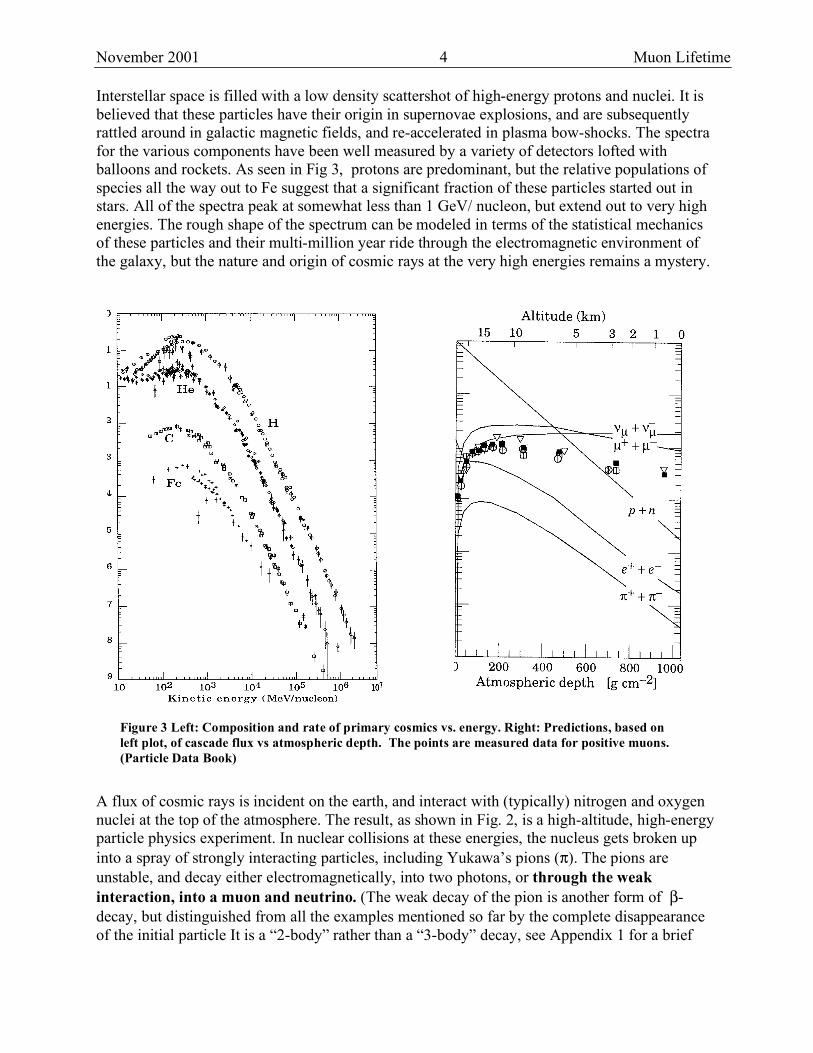
Interstellar space is filled with a low density scattershot of high-energy protons and nuclei. It is believed that these particles have their origin in supernovae explosions, and are subsequently rattled around in galactic magnetic fields, and re-accelerated in plasma bow-shocks. The spectra for the various components have been well measured by a variety of detectors lofted with balloons and rockets. As seen in Fig 3, protons are predominant, but the relative populations of species all the way out to Fe suggest that a significant fraction of these particles started out in stars. All of the spectra peak at somewhat less than 1 GeV/ nucleon, but extend out to very high energies. The rough shape of the spectrum can be modeled in terms of the statistical mechanics of these particles and their multi-million year ride through the electromagnetic environment of the galaxy, but the nature and origin of cosmic rays at the very high energies remains a mystery.

Figure 3 Left: Composition and rate of primary cosmics vs. energy. Right: Predictions, based on left plot, of cascade flux vs atmospheric depth. The points are measured data for positive muons. (Particle Data Book)

A flux of cosmic rays is incident on the earth, and interact with (typically) nitrogen and oxygen nuclei at the top of the atmosphere. The result, as shown in Fig. 2, is a high-altitude, high-energy particle physics experiment. In nuclear collisions at these energies, the nucleus gets broken up into a spray of strongly interacting particles, including Yukawa’s pions (π). The pions are unstable, and decay either electromagnetically, into two photons, or through the weak interaction, into a muon and neutrino. (The weak decay of the pion is another form of β-decay, but distinguished from all the examples mentioned so far by the complete disappearance of the initial particle It is a “2-body” rather than a “3-body” decay, see Appendix 1 for a brief


explanation.) The particles from the pion decays, including a large number of muons, then make the rest of the trip down to sea level. Travelling at almost the speed of light, a muon with lifetime 2µsec will travel just under 600 meters before it decays. A significant flux exists at the bottom of the atmosphere because, in the rest frame of the earth (the lab frame), the muon lifetime is time-dilated. If the lifetime in the muon’s rest frame, the proper lifetime, is τ, and the muon has velocity β = v/c, the lifetime as measured in the lab frame will be

22

1, where

1lab

Et

mc!" !

#= = =

$

As seen in Fig. 4, most muons reaching the ground are very relativistic. A 10 GeV muon has γ ~1000, and therefore travels 600 km before it decays! As you can infer from Fig. 3, the number of muons reaching us at ground level is a shocking 100 per square meter per second. This is a significant fraction of the total radiation exposure for all people, and small but non-negligible occupational safety issue for airline personnel.

Figure 4 Sea level muon energy spectrum. Most of the flux at the ground is still highly relativistic.

Incidentally, notice in Fig. 3 that the depth of the atmosphere is measured in g cm-2. You should understand the reason for this. See Knoll, Leo, or Melissinos.


4. Experimental Detection of Cosmic Ray Muons In this experiment, we will detect time-dilated, high-energy muons as they mostly pass into and through a detector. A very small fraction stop in the detector, and then decay with something close to the proper lifetime. The electron from the decay creates signal similar to the initial muon. By using precision electronics to time the difference between pulses, we can isolate the muon decay signal as an excess of time differences at Δt ~ τ, with an exponential shape that measures τ. a) Scintillators One method for the detection of ionizing radiation is based on materials which convert the ionization energy into visible light, a.k.a. scintillators. These are as common as the video display, where the image is the result of an electron beam striking ‘phosphors’ on the inside face of the CRT. For particle detection with timing applications, the scintillators of choice are certain systems of organic molecules, which we employ here in liquid form. We use a tertiary liquid system. The primary element is 1-2-4 trimethyl-benzene, which is a precursor for the manufacture of polyester. Like many other organic scintillators, this compound is aromatic, and the carbon rings have molecular orbitals which are easily excited by a passing charge. This molecule does not radiate, but by a dipole-dipole exchange, passes the excitation on to the secondary component, which makes the light, a so-called fluor. Our fluor is 2,5-diphenyloxazole, otherwise known as PPO, gets excited, suffers a configurational change to a slightly different state on collision with nearby molecules, and then radiates back down to its ground state, with slightly different energy difference than the original excitation. This configuration change is important in order that the scintillator be transparent to its own scintillation light! Unfortunately the frequency of the light is in the UV, so a third component is added, a so called wave-shifter, which absorbs UV photons and then reradiates near 450 nm, where photomultipliers are typically sensitive. Our wave-shifter is known as bis-MSB. . The advantage of liquid scintillator is the ability to create systems with large coverage, as we need to measure the cosmic ray flux. The tertiary chemical system above is diluted in a base of transparent mineral oil. The approximate mixture is 90% mineral oil, 10% trimethyl-benzene, 0.1% flour and wavshifter, and a trace amount of BHT (the food preservative), yes “to prevent spoilage”. In other applications, the whole business gets fixed in plastic, and the scintillator is sold in large sheets. All of the re-radiation steps described above happen in nanonseconds, making organic scintillator a detector of choice for timing measurements. However, the light output is low, and the resolution on the actual amount of energy deposited is poor. Certain salts, such as NaI are so called inorganic scintillators, with much better energy resolution, at the expense of a much slower signal and poor timing resolution. A full description of the physics of scintillators can be found in Knoll, Leo, or Tsoulfanidis. b) Photomultipliers


The photomultiplier (PMT) is a tube device that functions as one channel image intensifier. Light falls on a photo-cathode, and electrons are emitted via the photoelectric effect. Some simple electromagnetic optics accelerates these electrons and directs them to the first in a series of surfaces, called dynodes, chosen from materials with good secondary electron emission. The dynodes are arranged mechanically so that adjacent dynodes are within millimeters of each other, and a single high voltage power input is directed down a resistor chain that maintains a potential difference of 50-100V between each pair of dynodes. In this arrangement, the photo-electrons create a larger shower of electrons off the first dynode, which creates a larger shower from the second dynode, and then a chain-reaction of electron emission flows down the tube, amplifying the size of the electron bunch at each dynode. Finally collected at an anode, amplifications of O(106) are typical, so if 1000 electrons leave the cathode, the final charge pulse is O(10-10C) The PMT gain is fixed by the dynode design and the applied high voltage. Small changes in HV lead to significant effects in gain, so good HV regulation is important. With the gain fixed, the tube output depends entirely on the number of electrons at the first step, and one of the key performance

Figure 5 Left: A typical PMT. Right: QE vs. frequency

issues for PMTs is the number of electrons produced per unit photon, this ratio is called the quantum efficiency. The Q.E. depends on the cathode material and the frequency of the radiation. Our tube has a bi-alkalai cathode, typical responses for these are shown on the right in Fig. 4. The bis-MSB scintillation peaks near 450 nm, so it’s a good match here, but in general there is always the design problem of matching cathodes to scintillators. One expects good cathode materials to have q.e.’s greater than or equal to 20% at the frequencies of interest. PMTs come in a variety of sizes and designs tuned to applications. Recent developments include large light collecting inputs, for use in detecting the Cerenkov radiation of solar and astrophysical neutrinos in huge underground water tanks, and our apparatus uses an early version of this kind of tube.


c. Electronics (See Addendum for updated diagram.) At this point in the signal chain, we have at the PMT anode a small charge pulse proportional to the energy deposited in the scintillator. The trick is now to measure the time difference between each pulse and the next. This is accomplished with some modular “NIM” electronics, as developed a past era of small scale of nuclear experimentation. This stuff is nowadays starting to look kind of quaint, but still has the great utility of being easy to mix-and-match, and also allowing inspection of each step in the signal chain. We will eventually have a glossary discussion of issues for signal processing and our electronics implementation in the lab. You can also find more detail in Knoll or in Tsoulfanadis. For now, briefly, the issues in our setup are as follows. The PMT output, a negative charge or current pulse, is sent to a discriminator, which outputs a standard “NIM logic pulse” if the input magnitude exceeds a certain threshold voltage. The discriminator allows us to reject a huge background noise rate of low voltage noise signals, because real signals are large enough to be “over threshold”. The output of the discriminator is then used to start or stop a clock inside the Time-to-Amplitude Converter (TAC), which outputs a voltage pulse proportional to the time difference between start and stop.

Figure 6 Schematic of the experimental set-up. (M. Longo)

Finally, this voltage is sent to an analog-to-digital converter (ADC) in the small black box, and the output of that is sent over the serial bus to the computer, which runs software with the plotting, histogram, and analysis package. You will accumulate a “spectrum” of voltage pulses each of which is proportional to a muon decay time. In the end, you should see an exponential distribution of the recorded pulse heights. It’s a pulse-height-analyzer: PHA. In the pre-computer days, the histogram function was done with a special purpose instrument like a big oscilloscope, which


could record data in many memory locations or channels (remarkable at the time), and hence was called a Multi-Channel-Analyzer. The jargon MCA has stuck, and that’s why our computerized analyzing device is called “Pocket-MCA”. We will also use a “scaler” to count pulses, and a pulse generator and a NIM “delay amplifier” to establish the time calibration. Note that part of the “NIM standard” is that all the boxes expect their outputs to be driving 50Ω. As long as you plug one box into another, you don’t have to worry about this. However, if you look at an output with an oscilloscope, you need to be sure that the scope looks like 50Ω looking in. For the scope you will use in this lab, this is accomplished by changing an internal setting. 5. Experimental Set-up a. Inspirational Prologue on Method This is one of those experiments that amounts to the measurement of a single important number. You are going to do it by making a timing measurement with accuracy on the order of 10-7 seconds. Think about that. A deep part of the experimenter’s craft in this case is to convince the world that you have understood and controlled your calibration, as well as the sources of error. So, instead of thinking about the tedious chore of error analysis as slapped together at the end, think of it as understanding your resolution, up front, as the heart of the measurement. Furthermore, note that if you want to measure a tenth of a microsecond, you cannot just hook everything together and hope for the best. You need to examine the signal each step of the way, to make sure everything is under control. b. The PMT Our detecting medium is mineral oil doped with scintillator, inside a 55-gallon drum. There are two tubes mounted looking down into the drum. A single cable from each tube goes to a “Bud Box”, where it picks up the HV, and where it hands off the scintillation signal. As of Fall 2001, one tube has a “light-leak”, is marked X, and should not be used. Trace the cable to see that you are using the right tube. In our tube, the cathode is at ground and the anode is at positive high voltage, which means the signal is coupled out through a big blocking capacitor. Other tubes in the lab, including a few demonstration models near the gamma bench, use a grounded anode scheme, so the cathode is at a negative high voltage. When connecting to HV supplies, check that you know what you need and what the supply produces, and don’t screw up. Connect the HV and step up to POSITIVE 1.5KV, pausing for a few seconds at each turn of the knob (the tube is happiest to charge up to the final HV “smoothly”, rather than in one big step).


This is a timing experiment, so use the 500MHz scope. Connect the tube output the scope. Use the scope channel control to terminate in 50Ω, in order to simulate the input impedence of the discriminator. Trigger the scope in “normal” mode on the channel you are using, and set a negative threshold starting at 10 mV or so. Look for negative going pulses with sharp risetime. Those are PMT pulses. The size of the pulse if determined by the light output of the scintillator, the efficiency of the optical coupling to the PMT, and the PMT gain. The length of the pulse is almost entirely due to the time constants of the scintillating processes. c. The Discriminator We use one channel of a “Lecroy Octal Discriminator”, the box with the blue front panel. This is made to accept the signals directly from PMTs, without any preamplification or termination. Tee the PMT signal at the scope, and send the signal into the input of the 2nd discriminator, the threshold on this channel is pre-set for you. Connect the discriminator output to the second channel of the scope, terminating in 50Ω. Diplay both the PMT and the discriminator output, trigger on the PMT, and find the discriminator output pulse. You may have to expand the scope time scale. What is the width of the discriminator logic pulse? Why does this make sense? Try triggering on the discriminator pulse. Where does it come in relation to the PMT pulse shape? If you are curious about this, check references. Plug a discriminator output into the scaler and measure the count rate. This is your raw muon rate. Compare to what you expect for the rate of muons at sea level, given our detector geometry. You may need to estimate the solid angle subtended by the detector. What is the mean time between pulses? Compare to muon lifetime. Why do you care? d. The Time-to-Amplitude Conversion and the Time Scale Calibration Recall our muon lifetime technique: Each muon entering the drum produces a pulse on arrival. If it stops and decays, the final state electron produces a pulse at death. If we could start a clock on the first pulse, and stop it on the second, we would have a lifetime measurement. Unfortunately, we have no way to know which of the pulses in the drum is a decay electron. So, we measure the time difference between every pair of pulses. We expect a Poisson distribution with a mean of 0.01 seconds (why?), but at much smaller times we expect to see a small excess population of time differences of order τµ. We process the time differences by converting them to voltages with the TAC. This device will put out a voltage between 0 and 10 V, proportional to the ratio of the input time difference and a “range” that you set on the front panel. Set the range to 8 µs, using the knob and the x10 switch. The voltage of the output then represents times from 0 to 8 µs and you are sensitive to the muon lifetime. What happens to the signal from pulse pairs that represent pass through muons arriving one after the other? To get the hang of this device, start with fake signals from the pulser. Look at the pulser signal with the scope, set up a train of narrow negative pulses separated by >> 8 µs. Tee the pulser output at the scope and run the signal into the delay amplifier. While triggering on the pulser, look at the


output of the delay amplifier on channel 2 of the scope. Change the delay. Verify that you can see the timing delay on the scope. This is ultimately going to be your time calibration signal. Can you measure it? How well? Now tee the pulser output at the delay amplifier, and run a cable from there to the TAC Start. Run the output of the Delay Amplifier to TAC Stop. The TAC has two outputs. The spigot with 1Ω output impedence seems to work better in this setup. Look at that output on Channel 2 of the scope, while continuing to trigger on the pulser on Channel 1. You should see a rectangular bipolar pulse whose amplitude is directly proportional to the programmed delay. Verify that this works by changing the delay. e. The Pulse Height Analyzer Plug the TAC output into the Pocket MCA. The black box is on if the red indicator light is lit. Log onto the PC. Find the folder “MCA8000 WIN32” and run the application PMCA. You should get a standard WIN application screen, with a large space for the histogram and, on the right, a column for display of counting statistics. When you start up, you will be asked whether to open an old data file, or connect to an MCA. Chose connect. If you get a stale spectrum from the last user, go to “MCA”, then “delete data”, which clears the spectrum, and “reset time”, which clears the counting statistics. Then do “start acquisition”, and you should see a spike grow very quickly. Change the delay. You should see the spike move. What is happening: The MCA is looks for an input voltage between 0 and 10V, and then digitizes. The accuracy of the digitization is specified by the number of “channels”, which is equivalent to the number of bins in the histogram. For instance, if you have chosen 1024 channels, then each bin of the histogram is 10V/1024 ~ 0.01 V wide; the result of each digitization is rounded to the nearest 0.01V, and the corresponding bin is incremented Play with the program, learn how adjust the display, fit the peaks, and save the output. Now, you need to calibrate the conversion from channel number to time. You want to change the settings on the delay amplifier and see how many channels the peak moves by. Consider the uncertainties here very carefully. Take more than 2 points. Save the files! Is the channel-to-time conversion linear over the whole spectrum? Do the peaks have a finite width? Does it matter? Do you have anything to gain by changing the number of channels? By the way, how well do you trust the time calibration on the delay box? (You checked this with the scope in Part d. above) How does this affect your plotting strategy?

6. Measurement of the Muon Lifetime a. Experimental Procedure The muon lifetime will be measured by using the time between the muon arrival and muon decay scintillations to start and stop the TAC. As outlined in Sec 4.d. we do this by measuring the time between every pair of pulses in the barrel. This is accomplished (cleverly) in our setup by using one output of the discriminator to STOP the TAC, and using another output of the same channel to


START the TAC after a delay of at least 20 nsec. Imagine there has been a long period (compared to 8 µsec) without a muon. Then a muon enters the barrel. The TAC gets a STOP, but it already is stopped. Then, after 20 nsec it gets a START. Then, if the muon decays, the STOP shows up in ~ 2 µsec. Think through a few other cases and convince yourself that this works. What sets the length of the delay? Connect two discriminator outputs to START and STOP. Use a long cable to provide the START delay. (The cable delays are listed on the cable. Compare to cable length and speed of light!) Look at the TAC output with the scope; if you set things up correctly to run with 8µsec range using the pulser, the you should see a voltage amplitude signal from muon decays in the same range. Connect the TAC to the MCA and start accumulating. You will see a much lower rate here than you did with the scaler. Why? Can you calculate the rate that you might expect? You should plan to leave the experiment run overnight in order to accumulate a good spectrum. With good statistics, you should get an obvious exponential distribution. Save the plot. For the purpose of presenting your data, a nice finesse is to now reconnect the pulser, and do the time calibration, overlaying the fixed time peaks onto your saved lifetime distribution. b. Data Analysis You need to fit the lifetime distribution to the hypothesis of exponential decay. Use your saved plot without superposed calibration peaks. The .MCA file is a text file, edit with NOTEPAD and you can easily find the binary pairs representing the bin data. Cut and paste that data into Origin or Igor. Examine the exponential hypothesis by plotting with a semi-log scale. Is it purely exponential? If not: is it more than one exponential? Is there a background with a different shape? Do any of these differences matter relative to your expected time resolution? Convert your scale from channels to time and calculate the time constant. Estimate your uncertainty, which depends on the statistics of your plotting and fitting, and also on the time calibration of the hardware. Note, as per Sec 5.a., that a thoughtful analysis of the uncertainty is the whole art of this measurement. Compare your result to the known muon lifetime and comment on the level of agreement. 7. References Fraunfelder and Henley, Subatomic Physics, is an interesting all purpose book about particle and nuclear physics, but the treatments are very uneven. It has a nice overview of cosmic ray physics in Chap. 19. Chap11 is a somewhat high level discussion of the weak interaction, with muons. The Particle Data Book, Sec. 20 has a technical but accessible overview of cosmic ray physics.


G. Knoll, Radiation Detection and Measurement has everything: radiation interactions in Sec. 2, scintillators in Chap. 8, PMTs in Chap. 9, and Pulse electronics in Chap 16 and 17. Q. Leo, Techniques for Nuclear and Particle Detection is complementary to Knoll. A. R. Melissinos, Experiments in Modern Physics has a nice derivation of the energy loss of charged particles in Chap 5. N. Tsoulfanidis, Measurement and Detection of Radiation, is similar to Knoll or Leo. You should look at all three of these and see which one you like.

measurement of the muon lifetime - university of...

Documents