1

MEASUREMENT PROTOCOL OF ABSORPTION BY CHROMOPHORIC DISSOLVED ORGANIC MATTER (CDOM) AND OTHER DISSOLVED MATERIALS By the CDOM Working Group Antonio Mannino1, Michael G. Novak1,2, Norman B. Nelson3, Mathias Belz4, Jean-François Berthon5, Neil V. Blough6, Emmanuel Boss7, Annick Bricaud8, Joaquin Chaves1,2, Carlos Del Castillo1, Rossana Del Vecchio9, Eurico J. D’Sa10, Scott Freeman1,2, Atsushi Matsuoka11, Richard L. Miller12, Aimee Neeley1,2, Rüdiger Röttgers13, Maria Tzortziou14, Jeremy Werdell1 1. NASA Goddard Space Flight Center Greenbelt, MD, USA 2. Science Systems and Applications, Inc. (SSAI), Lanham, MD, USA 3. Earth Research Institute University of California Santa Barbara, CA, USA 4. World Precision Instruments Germany, GmbH, Friedberg (Hessen), Germany 5. Joint Research Centre of the European Commission, 21027, Ispra, Italy 6. University of Maryland, Department of Chemistry and Biochemistry College Park, MD, USA 7. University of Maine Orono, ME, USA 8. Laboratoire d'Océanographie de Villefranche (LOV), Sorbonne Universités, CNRS,

Villefranche-sur-Mer, France (retired) 9. Earth System Science Interdisciplinary Center, University of Maryland College Park,

MD, USA 10. Department of Oceanography and Coastal Sciences, Louisiana State University,

Baton Rouge, LA, USA 11. Takuvik Joint International Laboratory (CNRS-ULaval), Laval, Quebec, QC, Canada 12. Department of Geological Sciences and the Institute for Coastal Sciences and Policy

East Carolina University, Greenville, NC, USA (retired) 13. Institute of Coastal Research, Center for Materials and Coastal Research Geesthacht,

Germany 14. City College of New York (CCNY), City University of New York, NY, USA Citation for this document: Mannino1, A., M. G. Novak1,2, N. B. Nelson3, M. Belz4, J.- F. Berthon5, N. V. Blough6, E. Boss7, A. Bricaud8, J. Chaves1,2, C. Del Castillo1, R. Del Vecchio9, E. J. D’Sa10, S. Freeman1,2, A. Matsuoka11, R. L. Miller12, A. R. Neeley1,2, R. Röttgers13, M. Tzortziou14, and P. J. Werdell1 (2019) Measurement protocol of absorption by chromophoric dissolved organic matter (CDOM) and other dissolved materials, In Inherent Optical Property Measurements and Protocols: Absorption Coefficient, Mannino, A. and Novak, M. G. (eds.), IOCCG Ocean Optics and Biogeochemistry Protocols for Satellite Ocean Colour Sensor Validation, Volume ###, IOCCG, Dartmouth, NS, Canada.

2

This document is a product of a multi-year effort including a two-and-a-half-day workshop organized by the NASA Ocean Ecology Lab Field Support Group and hosted at NASA Goddard Space Flight Center in Nov. 13-15, 2013 and several CDOM absorption measurement round robins between November 2013 and February 2015 with significant international participation. The resulting protocol document, Measurement Protocol Of Absorption By Chromophoric Dissolved Organic Matter (CDOM) and Other Dissolved Materials, and the associated working group activity were sponsored by the National Aeronautics and Space Administration (NASA) including funding for the Field Support Group (NASA Ocean Biology and Biogeochemistry Program) and a 2012 ROSES proposal to Richard Miller, Norm Nelson, Carlos Del Castillo, Antonio Mannino and Jeremy Werdell under NASA Program Topical Workshops, Symposia, and Conferences with additional support for contributing authors and workshop participants by their respective institutions (see Appendix C for complete list of workshop participants). This document represents an update to the 2003 NASA Technical Memorandum, providing a detailed discussion of the state-of-the-art technologies and protocols for collecting water samples and measuring the absorption coefficients of CDOM. Important contributions by all the authors over many years made the completion of this document possible. THE AUTHORS RESPECTFULLY DEDICATE THIS PROTOCOL DOCUMENT … To the memory of Rossana Del Vecchio, a great colleague and better friend. We miss her sorely. http://www.ioccg.org Published by the International Ocean Colour Coordinating Group (IOCCG), Dartmouth, NS, Canada, in conjunction with the National Aeronautics and Space Administration (NASA). Doi:

3

Table of Contents I.INTRODUCTION..............................................................................................................................................4II.MEASUREMENTPROTOCOLS.....................................................................................................................5SAMPLECOLLECTION,FILTRATION,ANDSTORAGE..........................................................................................................5

Pre-cruise preparations..............................................................................................................................................................5GENERALCONSIDERATIONSFORSPECTROSCOPY..............................................................................................................9REFERENCEMATERIALS...................................................................................................................................................10SAMPLEPREPARATIONFORANALYSIS............................................................................................................................13LIQUIDWAVEGUIDESPECTROSCOPY...............................................................................................................................13Preparationoftheinstrumentandsamplesforanalysis.......................................................................................13Measurementprocedure........................................................................................................................................................16UltraPathandLWCCeffectivepathlengthdetermination....................................................................................21

DOUBLEBEAMSPECTROSCOPY(1,5OR10CMCUVETTES)–PROCEDURE................................................................22............................................................................................................................................................................................28SEA-BIRDSCIENTIFICABSORPTION-ATTENUATION(AC)METERS–LABORATORYPROCEDURE...............................28DISCRETEMEASUREMENTSOFCDOMABSORPTIONFROMINTEGRATINGCAVITYABSORPTIONINSTRUMENTS....30INSITUVERTICALPROFILESANDUNDERWAYMEASUREMENTAPPROACHES............................................................30VerticalProfileCDOMAbsorptionMeasurements....................................................................................................30Ship-basedunderwayflow-throughCDOMAbsorptionMeasurements.........................................................31

III.DATAANALYSISANDERRORBUDGETS.............................................................................................31EXAMPLEERRORBUDGET.................................................................................................................................................32

IV.DATAREPORTING....................................................................................................................................35V.EVALUATIONOFFILTERMATERIALSFORCONTAMINATION.......................................................36BACKGROUND....................................................................................................................................................................36METHODS...........................................................................................................................................................................36RESULTS.............................................................................................................................................................................37

VI.CDOMABSORPTIONMEASUREMENTROUNDROBINRESULTS...................................................40Table2.CDOMabsorbanceRoundRobinparticipantsandtheinstrumentationusedinthecomparison....................................................................................................................................................................................44

REFERENCES.....................................................................................................................................................45APPENDIXA:WPIADVANCEDFLOWCELLCLEANING...........................................................................50APPENDIXB:CONSENSUSCDOMABSORPTIONCOEFFICIENTVALUESOFSUWANNEERIVERFULVICACIDI(SRFA-I)SOLUTIONS...........................................................................................................52

TableB1.CDOMabsorptioncoefficientvaluesforSRFA-I0.25mgL-1solutionfromtheFebruary2015RoundRobinmean,medianand2.5%and97.5%quantilevalues......................................................52TableB2.CDOMabsorptioncoefficientvaluesforSRFA-I0.50mgL-1solutionfromtheFebruary2015RoundRobinmean,medianand2.5%and97.5%quantilevalues......................................................63

APPENDIXC.NOVEMBER2013CDOMWORKINGGROUPWORKSHOP...........................................74

4

I. Introduction Light absorption by chromophoric dissolved organic matter (CDOM) dominates the ultraviolet (UV) and short wavelength blue portions of the absorption spectrum in all aquatic environments, thus exerting primary control on photochemistry, photobiology, and ocean color. In order to produce valid results, ocean color models (e.g., in situ or remote sensing-based radiative transfer or bio-optical inversion models) must take into account the absorption spectrum of CDOM. Measuring light absorption by CDOM in situ is a necessary condition for developing and validating current and future ocean color algorithms for all applications. We are revising this section of the NASA ocean optics protocols (Mitchell et al. 2003) under the auspices of the International Ocean Colour Coordinating Group to reflect the development of new instrumentation and a greater understanding of the importance of CDOM and its distribution in coastal and open ocean waters over the past twenty years. Our goal here is to develop a set of procedures that will be adhered to by the ocean optics community for making CDOM measurements that can be integrated into NASA’s bio-optical database (currently named the SeaBASS) or similar databases, of sufficient quality to develop and validate ocean color algorithms and contribute to CDOM science. An overview of the absorption coefficient of CDOM and particles for pure and natural waters is described in another protocol document (Twardowski et al. 2018). The relevance of CDOM absorption measurements for satellite and airborne remote sensing applications is constrained to the Earth-surface solar radiation wavelength range (>280 nm). For the purposes of this discussion “CDOM” is operationally defined as material that passes through an approximately 0.2 µm pore-size filter and absorbs light at wavelengths above 250 nm. This material is predominantly composed of organic molecules (hence the CDOM nomenclature), nevertheless, inorganic constituents such as nitrate, bisulfide, dissolved iron, and so-called colloids or nanoparticles of iron oxides and minerals contribute to (and interfere with) absorption measurements of organic molecules (e.g., Zafiriou et al. 1984; Johnson and Coletti 2002; Weishaar et al. 2003). The absorption by inorganic constituents such as nitrate, nitrite, bisulfide, iodide, bromide, etc. becomes pronounced at wavelengths below 250 nm (Johnson and Coletti 2002; Birkmann et al. 2018). Measuring light absorption at shorter wavelengths is useful for characterization of the composition of CDOM and assessment of mineral ion concentrations, but does not play a direct role in ocean color, photochemistry, or photobiology. This operational definition permits colloids and smaller particles (such as some viruses or fragments of organisms) to be considered part of the CDOM, but does not operationally separate out absorption by nitrate and mineral ions particularly at wavelengths below 350 nm. The main characteristic of typical CDOM absorption spectra is an approximately exponential decline with increasing wavelength. Absorption at 300 nm can be a factor of fifty higher than at 500 nm. Conventional absorption spectroscopy using 1 cm or 10 cm cuvettes can resolve CDOM absorption in the UV, but not the visible, in the oligotrophic ocean and some offshore coastal areas. In order to validate most ocean color products, we must be able to accurately measure CDOM absorption spectra in the visible with

5

known uncertainties. We have focused our efforts on new technologies now commercially available, in particular liquid waveguide cells, which can have pathlengths up to 200 to 500 cm. These new technologies come with greater capabilities but also have unique problems and considerations. The current edition of these protocols summarizes our current state of knowledge and provides recommendations for how to make accurate and precise measurements going forward. In most cases our recommendations are based on and reflect the previous protocols (Mitchell et al. 2000; 2003). We have tried to highlight those cases where we have made a significant revision to the protocol.

II. Measurement Protocols

Sample Collection, Filtration, and Storage When measuring trace organics, it is necessary to minimize organic contamination of the samples during collection. Procedural ultrapure water blanks should be prepared to monitor potential contamination through each step of the sampling, filtration, and storage procedure including from Niskin bottles (or any other water sample collection method), filters, filtration apparatus, handling, sampling and storage containers, and through the shipping and storage process. This is necessary to achieve an end-to-end uncertainty budget. Pre-cruise preparations • Sample bottles (amber glass bottles with Teflon-lined caps) used to collect CDOM

samples or to store ultrapure standard reference water need to be thoroughly cleaned to remove any potential particulate and organic contaminants. The recommended bottle and cap cleaning procedure1 entails sequential soaks and rinses in dilute detergent, purified water (deionized Type II), and 10% HCl, followed by final copious rinses with ultrapure water2 (5 or more rinses). Alternate bottles may be used but should be evaluated prior to use for each specific application (e.g., oligotrophic ocean water, river water, etc.).

Note: The original protocols recommended clear Qorpak® glass bottles. However, this protocol recommends amber glass bottles to mitigate UV exposure and thus potential photooxidation of samples during sample processing, storage, and preparation for analysis. Lab experiments have demonstrated no measurable contribution of CDOM to ultrapure water contained in these types of bottles for over 2 months of exposure (Fig.1).

• Dry bottles and caps in dedicated clean oven at 60°C for 4-12 hours. • Combust bottles with aluminum foil covers at 450°C for 6 hours. • Ultrapure water reference materials are prepared by rinsing combusted bottles and

caps and filling with fresh ultrapure water directly from the water production unit. Store in the dark.

• These reference water standards can be used to evaluate the quality of the ultrapure water produced at sea2 or as a replacement if ultrapure water is not available.

6

Sample Collection Samples should be collected from clean1 Niskin or Go-Flo bottles (silicone coated internal springs), using clean, non-contaminating, and non-absorbing/adsorbing high-purity tubing on the bottle outlet such as platinum-cured silicone, certain Tygon® formulations (2275, 2375, 2475) or fluoro-polymers (PFA, PTFE, ETFE). Samplers should wear powder-free non-latex gloves (such as nitrile) while handling samples, though gloves should not come into contact with the sample itself. Before filtration, the sample bottles used to collect whole water from the Niskin or Go-flo bottles should be rinsed three times prior to filling.1 CDOM measurements on samples collected from an underway flow-through system should be compared with results from Niskin bottle samples. Filtered CDOM samples may be collected directly from the Niskin or Go-Flo bottles using gravity filtration and an appropriate filter after adequate flushing (see section V for discussion on capsule filters). Triplicate samples, from randomly selected depths, should be collected daily – more frequently if a large number of casts are to be collected each day. The Goddard Space Flight Center (GSFC) High Performance Liquid Chromatography (HPLC) pigment project recommends replication at a rate of 10% of samples for phytoplankton pigments, and this is a worthwhile goal for CDOM absorption measurements. Samples from Niskin bottles that break the surface at the time of sampling should be distrusted because of potential contamination from a surface film with enhanced CDOM (e.g., Obernosterer et al. 2008; Tilstone et al. 2010). The distance from the pressure

1 For Niskin or Go-Flo bottles, “clean” refers to bottles that have been used multiple times and soaked in de-ionized water prior to the beginning of the cruise. Plasticware and glassware should be cleaned by soaking overnight in alkaline detergent bath (such as RBS™ 35), rinsing with reverse osmosis (Type-II) water, soaking in ~10% hydrochloric acid (HCl; 1.2M) bath overnight followed by copious rinsing (5 times or more) with ultrapure water2. Glassware should be baked at 450ºC for at least 6 hours.

Figure 1. CDOM absorption coefficient spectra (aCDOM(𝜆)) of ultrapure water stored in amber glass bottles in the dark at 4°C and analyzed periodically on a double beam spectrophotometer with 10 cm quartz cell to test for leaching of colored material. Note - the Day 19 (light green) spectrum is more representative of typical instrument noise than the other spectra.

7

sensor to the center of the Niskin bottles should be measured on a CTD rosette package in order to monitor whether the bottles were too close to the sea surface microlayer when they were sealed. It has also been demonstrated that at-sea lubrication of the rosette cable will contaminate CDOM and DOC samples for a considerable time (~10 deep-ocean casts) after the lubricant is applied (Nelson and Carlson unpublished data). Hence, precautions should be taken to prevent or minimize potential contamination of samples. CDOM samples are prepared by gentle vacuum filtration (<16.9 kPa, which is equivalent to <5 inches of mercury and <127 torr) or gravity filtration or through positive pressure filtration (<69 kPa or <10 psi) (see Figure 2 for example clean sample filtration apparatus). Samples should be filtered immediately following collection of the whole water sample. Note that impacts to CDOM absorption coefficients from delays in filtration are not well documented but could be important. It is preferable to use clean (acid washed and/or combusted) glass filtration apparatus either with stainless steel frits or glass frits. These should be rinsed with ~10% Hydrochloric acid (HCl) and ultrapure water2 after daily uses and acid soaked (in the case of glass frits) with longer intervals between uses. Sample filtrates should be collected in clean (see above) brown (amber)

2 Ultrapure water (Type I; resistivity ≥18.2 MΩ cm, <5 ppt TOC) that is ultraviolet oxidized and 0.2 µm-filtered water with total organic carbon ≤10 µg C L-1 (e.g., Milli-Q Gradient, Nanopure Diamond UV, etc.) for preparation of all solutions (acids, consensus reference material), rinsing, cleaning of spectrophotometer cells, and serves as the blank and reference. Water purification systems require diligent system maintenance to ensure high quality laboratory water with low CDOM and total organic carbon (TOC). Several manufacturers equip ultrapure water systems with TOC monitors that provide an indication of the carbon content of the water.

Figure 3. Diagrams of example filtration apparatus for collection of clean sample filtrate directly into sample bottle for measurement of absorption coefficients of the dissolved fraction nominally defined by the filter pore size. (a) Kontes filter dome and common glass filtration apparatus and (b) custom apparatus with Gelman plastic filtration equipment (diagram from Mitchell et al. 2000).

8

glass bottles or covered clear glass bottles with teflon cap liners. The NASA Ocean Optics Protocols did not recommend amber glass bottles due to a concern of contamination from the tinted glass to soluble absorption (Mitchell et al. 2003). However, testing of cleaned amber glass bottles demonstrate that these bottles do not introduce contaminants that interfere with CDOM absorption (Fig. 1). Sample bottles should be rinsed with filtered water three times before filling. Prior to sample filtration and after setup on the filtration apparatus, filters should be rinsed with ultrapure water and then rinsed with sample that is then discarded before filtration (minimum total volume of 175 to 200 mL is recommended for 47 mm diameter disc filters). If ultrapure water is not available, then sample water alone can be used. Acceptable filter types have effective pore sizes of 0.2 µm for coastal and open ocean waters, whereas 0.45 µm pore size filters are commonly used in freshwater systems and acceptable due to the practicality of working with high particle load samples. Acceptable membrane filter types for disc filters include glass fiber, polycarbonate (PC), polyethersulfone (PES), nylon and hydrophilic polypropylene (GHP) (see Section V for details). Nylon, Versapor and PureFlo SZL PES capsule filters, and GHP syringe filters were evaluated and are also deemed acceptable if adequately flushed with sample or a combination of ultrapure water and sample at the time of sample filtration (see Section V for details). The flushing volume seems to be critical to remove chromophoric and non-chromophoric organic contaminants. In heavy particle load situations, pre-filtration with combusted, rinsed glass fiber filters such as GF/F (manufacturer reported nominal pore size of 0.7 µm) can be used to prevent 0.2 µm filter clogging. Combusted Advantec GF-75 glass fiber filters, which have a manufacturer reported nominal pore-size of 0.3 µm, provide results comparable to the other membrane filters. An ideal filtration protocol to follow would involve pre-filtration of samples with an appropriate pore size filter for the particle concentration of the water sample and final filtration with an acceptable 0.2 µm filter prior to analysis. See section V for discussion on different filter types. For analysts aiming to quantify absorption spectra of both CDOM and particles, an important consideration is avoiding a gap across the size spectrum. Discrete measurements of particle absorption are performed on GF/F filters, which results in a gap in measurement between <0.2 µm CDOM fraction and the >0.7 µm particles. One possible solution is to utilize the GF-75 filters for particle absorption to reduce and potentially eliminate the possibility of a measurement gap. Comparisons of such discrete measurements with whole water absorbance spectrometers would verify the efficacy of filter choices across all natural waters analyzed. Samples should be stored in the dark in sealed bottles at ~4°C in a clean environment, and analyzed as soon as possible, preferably within 4 to 24 hours, but no later than within 6 months of collection (see results in Section VI) as it is not always practical to analyze samples at sea. Figure 3 is an example of a low absorbing CDOM sample stored in this manner that does not exhibit a change in absorption. However, this may not always be the case; temporal variability in CDOM absorption is likely dependent on sources and composition of CDOM. Freezing samples is generally not recommended (Fellman et al. 2008). Nevertheless, this storage approach may extend the storage period if loss in CDOM due to flocculation can be avoided.

9

General Considerations for Spectroscopy Spectrophotometers should be calibrated prior to analysis of a large batch of samples and annually at a minimum to ensure their accurate photometric performance. If available, the automatic calibration of the spectrophotometer for checking wavelength and slit size should be initiated. Neutral density filters traceable to NIST 930e are recommended for visible spectroscopy and liquid samples traceable to NIST 935a for ultraviolet spectroscopy. For assessing wavelength accuracy, the use of solid-state holmium oxide filters is recommended. NIST-traceable standards are available in various formats that can be immediately used in most double or single beam spectrophotometers. Spectrophotometer performance using NIST-traceable standards is a service that is provided by some spectrometer manufacturers as part of routine maintenance.

Figure 4. CDOM absorption coefficient spectra for a low absorbing CDOM water sample collected in the south Pacific measured shortly after collection with an UltraPath UPUV system with 200 cm liquid waveguide capillary cell and with the same instrument over 6 months later in the lab plotted on a linear (a) and logarithmic absorption coefficient scales (b) and (c) demonstrating no change in values within uncertainty of the measurement. Dates in the legend are shown in yyyymmdd format.

Figure 5. CDOM absorption coefficient spectra for a low absorbing CDOM water sample collected in the south Pacific measured shortly after collection with an UltraPath UPUV system and with the same instrument over 6 months later in the lab plotted on a linear (a) and logarithmic absorption coefficient scales (b) and (c) demonstrating no change in values within uncertainty of the measurement.

10

Calibration certificates from these exercises should also be provided to the bio-optical databases (e.g., SeaBASS) as part of the documentation. In addition to photometric calibration, liquid waveguide instruments must have their effective pathlength determined using a solution of known concentration and known extinction coefficient at a particular wavelength. This is typically performed by the manufacturer but must also be performed by individual labs to verify and repeated at least annually.

Reference Materials Ultrapure water serves as the standard reference water blank in CDOM absorption analysis. The importance of ultrapure water as the reference water blank for CDOM analysis cannot be overstated. Good results have been obtained from ultrapure water systems producing Type I water with low DOC2. Filter cartridges in ultrapure systems should be of the “low DOC” variety. Ultrapure water from the system must be filtered (0.2 µm) before use – most systems have this as the final filtration step. Quality of the prepared ultrapure water should be checked periodically by comparing to independent sources or comparison with past measurements. For routine work, Fisher Optima grade water (or comparable) tends to provide consistent results. It can be confirmed that a new cartridge filter set up is clean and working properly by zeroing the spectrophotometer using the Optima water and then measuring the absorption spectrum of ultrapure water from the system. Optima water does yield a small absorption signal in the UV. Routine analysis of DOC concentration of the ultrapure water can also be used to verify the quality of ultrapure water production system (on the order or 5-10 µg C L-1). Some ultrapure water units have built-in total organic carbon (TOC) modules for detecting degradation in water quality. However, it is recommended not to rely solely on readings from TOC units. One of the factors that enabled researchers studying DOC to have confidence in their measurements in recent years has been the availability of suitable reference material that can be analyzed along with samples. We are requiring as part of the standard protocol, measurement of the absorption spectrum of solutions of Suwanee River Fulvic Acid (SRFA) dissolved in ultrapure water, as part of each session of routine CDOM absorbance measurements. The intent is for CDOM analysts to use SRFA solutions to verify that their measurement process including instrument performance generates absorption coefficient values consistent with values provided in this protocol (Fig. 4). If results do not match, then the analysts should evaluate their instrument, measurement technique, and computations. SRFA-I standards in powder form are available from the International Humic Substances Society, St. Paul, Minnesota (https://humic-substances.org/ ). Currently, we recommend the use of the SRFA Standard I (SRFA-I; catalog # 1S101F; prepared 2003; US$125 for 100mg)3 in the following concentrations: 3 Future protocol revisions will specify an alternate SRFA Standard once IHSS no longer provides SRFA-I or batch 1S101F.

11

Figure 6. CDOM absorption coefficient spectra of (a) 0.25 mg L-1 Suwanee River Fulvic Acid I (SRFA-I) solution and (b) 0. 50 mg L-1 SRFA-I analyzed on 12 UltraPath UPUV and Liquid Waveguide Capillary Cell (LWCC) instruments and multiple double beam spectrophotometers from a multi-investigator round robin conducted in February 2015 – see Table 2 for details on instrumenation. UltraPath UPUV and LWCC data extend only between 300-700 nm. Data below 300 nm are from the double beam spectrophotometers. Measurements below 300 nm in the plots were made over time on the Round Robin SRFA-I solution. The 95% semi-interquantile ranges shown in black represent the variability in measurements between instruments and investigators. Tables B1 and B2 in Appendix B contain the tabulated values presented in these two plots.

Figure 7. CDOM absorption coefficient spectra of (a) 0.25 mg L-1 Suwanee River Fulvic Acid I (SRFA-I) solution and (b) 0. 50 mg L-1 SRFA-I analyzed on 12 UltraPath UPUV and Liquid Waveguide Capillary Cell (LWCC) instruments and multiple double beam spectrophotometers from a multi-investigator round robin conducted in February 2015. UltraPath UPUV and LWCC data extend only between 300-700 nm. Data below 300 nm are from the double beam spectrophotometers. Measurements below 300 nm in the plots were made over time on the Round Robin SRFA-I solution. The 95% semi-interquantile ranges shown in black represent the variability in measurements between instruments and investigators.

12

1 mg/L – for use with 1 cm cuvettes 0.5 mg/L – for use with long pathlength liquid waveguide cells and 10 cm cuvettes 0.25 mg/L – for use with long pathlength liquid waveguide cells and 10 cm cuvettes SRFA-I solutions should be thoroughly mixed and 0.2 µm filtered before use. Because the absorption response should be linear with concentration, plotting SRFA-I concentration versus absorption coefficient provides a rapid verification that SRFA-I solutions are prepared properly and the instrumentation is functioning properly. Analysts should verify that the SRFA-I solutions measured do not exceed the dynamic range of the double beam spectrophotometer or the liquid waveguide-pathlength combination. SRFA-I solutions should be stored at 4°C within amber glass bottles in the dark between uses. The powder can be stored long-term in a freezer such as at -20°C to -80°C to minimize degradation. Experiments are still being carried out to determine the useful lifetime of a given solution and for the SRFA-I powder (see Section VI for details). The date of preparation of all solutions should be recorded, and reported with results, so the community can compile data on storage effects, etc. Long-term storage and analysis of SRFA-I solutions reveal minimal changes in the absorption properties of the 0.25 mg L-1 SRFA-I solution (Fig. 5). From a stock solution of SRFA-I prepared on February 2, 2015 and periodically re-filtered and measured over 19 months, there was no significant change in absorption throughout the visible and UV spectral regions.

Figure 8. Evaluation of long term storage effects of SRFA-I solution (0.25 mg L-1) on CDOM absorption coefficients measured on a double beam spectrophotometer over a 19-month period plotted on a linear (a) and logarithmic absorption coefficient scales (b) and (c) demonstrating no change in values within uncertainty of the measurement. Dates in the legend are shown in yyyymmdd format.

Figure 9. Long term storage effects of SRFA-I solution (0.25 mg L-1) on CDOM absorption coefficients measured on a double beam spectrophotometer over a 19-month period plotted on a linear (a) and logarithmic absorption coefficient scales (b) and (c) demonstrating no change in values within uncertainty of the measurement. Dates in the legend are shown in yyyymmdd format.

13

When submitting data to SeaBASS or similar databases, it is required or recommended that researchers report mass and pathlength normalized decadal absorbance spectra (L g-1 cm-1) of SRFA-I solution with each batch of CDOM samples that have been measured as well as the date of preparation (Tables B1 and B2 in Appendix B).

Sample Preparation for Analysis All samples, blanks, and reference material should be equilibrated to a constant room temperature (±2°C) before analysis, typically standard room temperature, or other appropriate temperature for the sample such as 4°C for polar water samples, but only if the instrumentation is located in a chamber with a comparable temperature as the samples. The stability of the room temperature and the difference in temperature between sample and the reference water blank are the critical factors. Matching the temperature between reference and sample in conventional short pathlength spectrophotometers reduces the depression seen in the near-infrared region of the absorption curve, which is due to the temperature dependence of pure water absorption coefficients in this part of the spectrum (Pegau et al. 1997). This is of particular importance with the long-pathlength liquid waveguide cells, where small refractive index differences between the sample and blank can lead to significant errors. Fluctuating room temperatures can also affect the performance of the instrumentation. Samples stored for an extended period prior to analysis (more than several hours) should be re-filtered through a 0.2 µm filter as described in the Sample Collection section.

Liquid Waveguide Spectroscopy The liquid waveguide classes of instruments, which include the UltraPath and liquid waveguide capillary cells (LWCC), are composed of three instrument modules: a light source, a liquid waveguide capillary cell with 2 m or other pathlengths, and a spectrometer to detect the light transmittance through the two ends of the waveguide cell (Fig. 6). The protocol that follows is based on the assumption that CDOM analysts are familiar with operating liquid waveguide instrumentation and have received training from the instrument manufacturer or other expert. The protocol focuses on the use of an UltraPath system and its proprietary software. In case other systems (LWCC) and software are used, the protocol needs to be adapted in an appropriate way. Preparation of the instrument and samples for analysis Equilibrate samples, ultrapure water blanks, and reference materials to a constant

room temperature Turn on the light source and spectrometer unit at least 30 minutes before collecting

measurements. Recent studies have shown that lamps may take two to three hours to stabilize (Cartisano et al. 2018). However, such a long warm-up period may be indicative of aging lamps or unfavorable environmental laboratory conditions.

14

The flow rate of the peristaltic pump should be ~10 mL per minute on the UltraPath;

the WPI Peri-Star Pro peristaltic pump with 0.5 mm inner diameter tubing set at 30 RPM will achieve this rate. For the LWCC system, a lower flow rate of 1-2 mL per minute would be appropriate. When measuring samples or other solutions, fill the cell until the signal is stable and then stop the flow before collecting multiple scans. Analyst may also collect measurements in continuous flow mode, and preferred for LWCC systems (Lefering et al. 2017).

A 0.2 µm syringe filter can be added to the injection line may increase measurement stability. Recent work suggests that this may reduce the formation of microbubbles that can cause a bias in measurements. However, the syringe and filter should be thoroughly rinsed by injecting ultrapure water into the instrument until there is no measurable difference between syringe-filtered and non-syringe-filtered ultrapure water (Lefering et al. 2017).

Clean the waveguide cell according to the following procedure and in the order listed: o Load cell with a 10% solution of Contrad NF (or an equivalent alkaline

detergent) in ultrapure water – let stand 5 minutes o Inject 3 injection volumes (ca. 5 mL each) of HPLC-grade methanol o Inject 3 injection volumes of 10% HCl in ultrapure water (~1.2 M HCl) o Flush 5 cell volumes with ultrapure water

Peristaltic pump

Light Source WPI D2H

Spectrometer

sample

waste

WPI Multi-Pathlength Liquid Waveguide Capillary Cell

2 cm

10 cm

50 cm

200 cm

Fiber Optic Cable

Fiber Optic Cable

Injection Port

Flow Outlet Fiber Optic Switch

& Output ConnectorFiber Optic Connector

Fiber Optic Input Connector

Fiber Optic CableTubing for SampleTeflon Capillary Cell

Figure 10. Schematic of the World Precision Instrument (WPI) UltraPath UPUV system, which includes the UltraPath absorbance sample cell (center) with four nominal optical pathlengths (2, 10, 50 and 200 cm), deuterium/tungsten light source (left), photodiode array spectrometer (right), and peristaltic pump.

Figure 11. Schematic of the World Precision Instrument (WPI) UltraPath UPUV system, which includes the UltraPath absorbance sample cell (center) with four nominal optical pathlengths (2, 10, 50 and 200 cm), deuterium/tungsten light source (left), photodiode array spectrometer (right), and peristaltic pump.

15

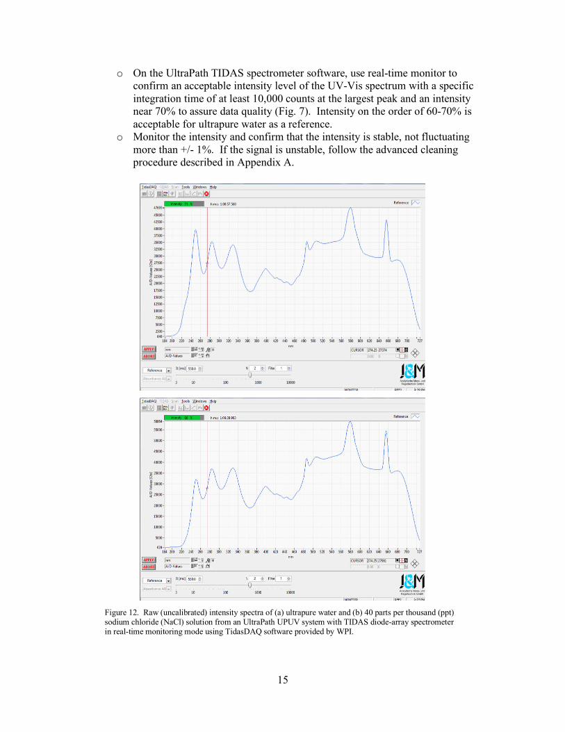
o On the UltraPath TIDAS spectrometer software, use real-time monitor to confirm an acceptable intensity level of the UV-Vis spectrum with a specific integration time of at least 10,000 counts at the largest peak and an intensity near 70% to assure data quality (Fig. 7). Intensity on the order of 60-70% is acceptable for ultrapure water as a reference.

o Monitor the intensity and confirm that the intensity is stable, not fluctuating more than +/- 1%. If the signal is unstable, follow the advanced cleaning procedure described in Appendix A.

Figure 12. Raw (uncalibrated) intensity spectra of (a) ultrapure water and (b) 40 parts per thousand (ppt) sodium chloride (NaCl) solution from an UltraPath UPUV system with TIDAS diode-array spectrometer in real-time monitoring mode using TidasDAQ software provided by WPI.

Figure 13. Raw (uncalibrated) intensity spectra of (a) ultrapure water and (b) 40 parts per thousand (ppt) sodium chloride (NaCl) solution from an UltraPath UPUV system with TIDAS diode-array spectrometer in real-time monitoring mode using TidasDAQ software provided by WPI.

16

Measurement procedure • After cleaning and flushing the cell with ultrapure water, stop the flow and close the

shutter on the light source. Wait a couple of seconds and then collect a dark reference spectrum.

• Open the shutter and wait a couple of seconds before measuring a light reference spectrum.

• Acquire 3 or more scans of ultrapure water to determine instrument noise and make a note of the reference intensity.

• Reload the ultrapure water blank into the waveguide capillary cell and acquire 3 scans to determine the error introduced by sample reinjection. The reference intensity for ultrapure water should be approximately 70% so that when a salty sample is introduced the intensity does not exceed 90%. Adjust integration times to stay within these limits (Fig. 7).

Note: The appropriate integration time varies significantly between instruments. The balancing of the lamps on the light source also affects integration time. As long as the counts are within the recommended range, then the user should be able to determine the appropriate integration time. It is necessary to check that for a given pathlength, the integration time is stable from one measurement series to the other. It should not vary by more than 5-10% over one month. A higher increase may indicate a problem either with the source or with the cleaning of the capillary tubing. Most critical is the stability of the integration time throughout the analysis of a sample set and should not vary by more than 1-2%. • Load 0.25 mg L-1 SRFA-I standard solution into the liquid waveguide cell and scan. • Reload and rescan if the signal at the long wavelength portion of the spectrum does

not reach zero, or the measured values exceed the 95% semi-interquantile range of the reported SRFA-I values (Figs. 4 and 27; Table B1).

o Refiltration of the SRFA-I solution may be necessary to obtain appropriate values. Ultimately, cleaning of the liquid waveguide capillary cell may be required if the expected values are not achieved.

It is recommended that analysts measure the apparent absorption spectra of sodium chloride (NaCl) solutions with salt concentrations that span the range of seawater salinity expected in their samples (e.g., 30 ppt and 40 ppt for open ocean samples; 15 ppt and 35 ppt for estuarine or coastal samples; etc.; ppt is parts per thousand and analogous to practical salinity units). NaCl is used here as equivalent to sea salt for simple practical reasons, it does not exactly represent sea salt and small differences compared to the effects of sea salt are expected. Analysts should utilize high-purity NaCl (e.g., Sigma-Aldrich Ultra, Acros, etc.) that has been combusted at 450°C for 4 hours. The saltiest solution should be weighed out and dissolved in ultrapure water in a volumetric flask and 0.2 µm filtered (e.g., 40.0 grams NaCl dissolved with ultrapure water up to the 1000 mL mark on a class A volumetric flask). This solution should be scanned in a spectrophotometer to check for contamination after filtration. Class A graduated cylinders can then be used to dilute the highest salt concentration to the required NaCl concentrations. It is good practice to check the salinity using a refractometer or other type of salinometer to confirm that the salinity of each solution is accurate.

17

Water absorption itself is changed by the presence of salt ions and dissolving such ions in water reduces the per volume amount of water molecules. As mentioned previously, liquid waveguide cells are sensitive to small changes in refractive index. The refractive index effect dominates in the blue-green portion of the spectrum, and water absorption effects dominate in the red and infrared spectrum. An increase in refractive index leads to higher light throughput (i.e., transmittance), resulting in negative apparent absorbance when a seawater sample is analyzed against ultrapure water as a reference (D’Sa et al. 1999; Miller et al. 2003). This effect has been reported to be spectrally variable (Nelson et al. 2007), to vary over time within a particular instrument (Nelson et al. 2010), and to vary between instruments (Figs. 8 and 9). In UltraPath 200 cm pathlength waveguide

Figure 15. Sodium chloride (NaCl) absorption spectra with negative slope measured on an UltraPath UPUV system (top) and the modeled spectra from the least squares linear fit (bottom).

Figure 16. NaCl absorption spectra with negative slope measured on an UltraPath UPUV system (top) and the modeled spectra from the least squares linear fit (bottom).

Figure 14. NaCl absorption spectra with positive slope measured on an UltraPath UPUV system (top) and the modeled spectra from the least squares linear fit (bottom).

18

cells, the magnitude of the effect has been reported to range from <0.001 to >0.003 optical density (OD) per ppt NaCl. Small but consistent offsets possibly related to refractive index have been reported for 10 cm cuvettes in spectrophotometers as well (Green and Blough 1994). There are different types of refractive index issues. For example, the refractive index also controls the transmission in the water-glass interface on both sides of a cuvette. The closer the index of refraction between the quartz and water (e.g., the saltier the water) the better the transmission. If ultrapure water is the reference water, differences in the sample salt content affect light transmission, which may or may not be negligible (see Boss et al. 2013). The UltraPath instruments tend to be stable when collecting multiple scans from the same injection (or loading) of a salty solution; however, reintroducing the same sample possibly produces absorbance spectra that vary significantly in shape and magnitude. Therefore, it is extremely important to “characterize” each UltraPath or LWCC system and create a set of salinity correction curves based on the behavior of each instrument at or near the time of analysis. It is strongly suggested that a minimum of three salt solutions are measured (such as 30, 35, 40 ppt) when generating a salinity correction curve. It is much easier to assess the accuracy of the NaCl solutions when comparing the shape and magnitude of three or more NaCl absorbance spectra (Figs. 8 and 9). Each salt solution should be injected three times and at least three scans collected per injection. While this may sound excessive, it is recommended to ensure that the salinity correction curves generated from these measurements will not be affected by contamination, bubbles (e.g., Lefering et al. 2017), or other unknown factors. By collecting multiple scans of a solution and also reinjecting the solution, it is less likely that a bad spectrum will be incorporated into the correction curve. Figure 10a shows an example of a 40 ppt NaCl solution that was continuously scanned for several seconds after injection into an UltraPath liquid waveguide cell. The instability is captured over the period of multiple scans that may be missed if only one of these spectra were measured. Figure 10b shows the same solution that was subsequently reinjected, and the variability of the scans was significantly less.

Figure 17. (a) Multiple scans measured in continuous mode collected within several seconds of each after loading a NaCl 40 ppt solution into an UltraPath UPUV 200 cm liquid waveguide system. (b) The same salt solution subsequently re-injected into the waveguide exhibiting significantly less variability between scans over a similar period of time.

Figure 18. (a) Multiple scans measured in continuous mode collected within several seconds of each after loading a NaCl 40 ppt solution into an UltraPath system. (b) The same salt solution subsequently re-injected into the waveguide exhibiting significantly less variability between scans over a similar period of time.

19

After measuring the salt solutions, calculate the mean and standard deviation of the multiple scans acquired for each injection. The standard deviation at all wavelengths should be less than 0.0007 absorbance units (AU) for the scans from each individual injection. If this criterion is met, then the averages from each injection may be compared. The spectral shape and the magnitude should be similar at all wavelengths. The standard deviation at wavelengths below 700 nm should be less than 0.002 AU and preferably less than 0.001 AU. If there is good agreement between the injections, then calculate their average; otherwise, discard any anomalous injections or repeat the procedure until spectra from at least two injections agree. The averages of the reinjections for each salt solution should be plotted to evaluate whether the shape of the absorbance spectrum from each salt concentration is similar. The amount of negative (or positive) offset of the NaCl solutions should be directly proportional to the salt content. The general slope of the absorbance spectra may be either positive or negative (higher or lower optical density with increasing wavelength) depending on the composition of the UltraPath liquid waveguide capillary cell as the manufacturer changed the Teflon formulation of the liquid waveguide capillary cell with a Teflon composition yielding a different refractive index (Figs. 8 and 9). If three salt solutions are analyzed, then at each 1 nm wavelength perform a linear fit with respect to salinity using a least squares regression approach (i.e., plot OD vs NaCl ppt at each wavelength and perform a linear regression analysis for each set of three points), the individual linear regression models of the NaCl spectra will account for any small variations in the shape of the measured spectra (Fig. 11). A(λ) = m(λ) * X + b(λ), where A = absorbance, X = NaCl salinity value, m = regression slope and b = y-intercept

Figure 21. Model of NaCl absorbance spectra using a least squares linear fit to the measured NaCl absorbance spectra. The linear fit is shown here at 5 nm intervals for clarity in the figure; however, the fit should be calculated at 1 nm intervals.

Figure 22. Model of NaCl absorbance spectra using a least squares linear fit to the measured NaCl absorbance spectra. The linear fit is shown here at 5 nm intervals for clarity in the figure; however, the fit should be calculated at 1 nm intervals.

Figure 19. Linear interpolation at 1 ppt increments (for visualization clarity) of the modeled NaCl absorbance spectra. In practice, the interpolation should be carried out at 0.1 ppt increments.

Figure 20. Linear interpolation at 1 ppt increments (for visualization clarity) of the modeled NaCl absorbance spectra. In practice, the interpolation should be carried out at 0.1 ppt increments.

20

Finally, absorbance values should be linearly interpolated at 0.1 ppt intervals for each 1 nm wavelength linear regression model (300-730 nm) (Fig. 12). If only two salt solutions are measured (three or more solutions are strongly recommended), perform a linear interpolation to the actual absorbance spectra at 0.1 units. Examples demonstrating the necessity of this procedure to properly attribute the refractive index offset from the sample salinity to the NaCl proxies for each type of waveguide capillary cell material are shown in Figures 13 and 14. From the results of multiple round robin exercises, it was found that the refractive index offset caused due to the salinity of natural samples tends to be inconsistent among different UltraPath systems and are not entirely due to the UltraPath capillary cell Teflon formulation (Figs. 13 and 14). After testing multiple methods to correct for this, the procedure that produced the strongest agreement between UltraPath systems was the following: • Measure NaCl solutions across a range of salinities that bounds the salinity of the

natural samples. • Generate a correction curve from these measurements. • Subtract the NaCl interpolated curve from the CDOM absorbance spectra that

produces a value close to zero at 685 nm4.

A simple way to find the optimal correction curve is to compute the absolute value of the difference between the sample absorption at 685 nm and all of the interpolated curve values at 685 nm. The interpolated curve that yields the minimum difference should be used for correction. The optimal NaCl curve may not match the salinity value of the seawater sample because NaCl solutions do not produce an identical refractive index response as seawater. Selecting the interpolated NaCl curve that best matches the null

4 The specification of this wavelength is justifiable because of the low absorption by CDOM and a plateau in the water absorption at 685 nm, and due to this plateau, the temperature and salinity effects on the water absorption are minimal at 685 nm.

Figure 253. NaCl and “Tahiti seawater” absorption spectra measured on a negative slope UltraPath system. The salinity of the Tahiti seawater was 34.7 ppt, but the offset measured is much closer to the offset from the 40 ppt NaCl solution at the red-end of the spectrum.

Figure 234. NaCl and “Tahiti seawater” absorption spectra for a positive slope UltraPath system. The salinity of the Tahiti seawater was 34.7 ppt, but the offset at the red-end of the spectrum falls between the 35 and 40 ppt NaCl values.

21

region refractive index response enables a better refractive index correction. The absorbance of all the samples measured between 650-700 nm should fall within the absorption bounds of the high and low NaCl solutions at the same wavelengths. If samples are outside these bounds, it is an indication that there may be a problem within the waveguide flow cell or that the salinity of the sample is not bounded by the salinity of the NaCl solutions. Once the SRFA-I and salt solutions have been measured and are within acceptable limits, the analysis of samples can begin. Approximately two cell volumes of ultrapure water should be injected and scanned (as a sample) before and after every sample to flush the cell and monitor system performance (at least two cell volumes or ~three minutes). If the reference signal is unstable it may be necessary to flush the cell with greater volumes. When analyzing a low CDOM absorption sample after a high CDOM sample, it is often insufficient to flush the cell only with ultrapure water; a complete cleaning avoids an overestimate of absorption coefficients over the entire spectrum. It is not necessary to conduct multiple injections on each sample; however, it is good practice to reinject at least one to three samples per analysis sequence to assure instrument stability. Analysts should inject sample replicates at this time, including procedural replicates (sampling, handling, filtering, etc.) to quantify the reproducibility of the absorbance spectra. The practitioner should avoid collecting new reference spectra during the analysis sequence. If there are signs of instability, such as the ultrapure water reference intensity varies more than +/- 2% of the initial value, try flushing the cell again with the cleaning solutions. If the reference intensity of the ultrapure water does not return to its initial value, it may be due to environmental changes in the surroundings. Thus, it may be necessary to collect new dark and light reference spectra. However, the reference intensity must be stable at the new value and new salt solution scans will need to be measured. If there are significant changes in the intensity of ultrapure water between samples, it is an indication that there is a problem within the cell. Most likely it is contamination or clogging within the cell causing bubble formation. If the intensity signal cannot be stabilized with the standard cleaning solutions, follow the advanced cleaning protocol described in Appendix A. When collecting new dark and reference scans, the filename must be changed or the previous scans will be overwritten. UltraPath and LWCC effective pathlength determination The effective pathlengths for each pathlength of the UltraPath capillary cell unit and LWCCs should be determined on a regular basis, especially after instrument returns from a field campaign. Several procedures can be employed to determine effective pathlength (Belz et al. 1999; 2006; Cartisano et al. 2018). Here we summarize one approach from Cartisano et al. (2018) using phenol red solutions as opposed to potassium dichromate (NIST 935a) solutions because the latter requires dissolution in perchloric acid5. The first step is to prepare a stock of phenol red solution (~16 µM) by dissolving phenol red (ACS

5 Over time, perchloric acid solutions can form perchlorate crystals such as on the rims of bottles or caps as well as within fume hood exhaust systems. Perchlorate crystals are explosive and can be detonated through friction, heat, fire, or impact with another object.

22

grade) with 0.05 M Tris-(hydroxymethyl)aminomethane (THAM; molecular biology grade) within a class A volumetric flask. From the stock, at least five separate solutions of phenol red should be prepared per UltraPath capillary cell pathlength to be evaluated and span the linear range of the concentration versus absorbance response, for example ~0.01 to 0.08 µM and ~0.01 to 0.3 µM for use on the 200 cm and 50 cm UltraPath capillary cell pathlengths, respectively (Cartisano et al. 2018). Because of impurities in commercially available phenol red, the actual concentration of phenol red should be determined using the molar absorption coefficient under well characterized temperature and pH conditions (Lai et al. 2016). For example, Cartisano et al. (2018) determined the actual concentration of phenol red at pH of 10.4 and 23°C using a 1 cm cuvette and a double beam spectrophotometer. The effective pathlength can be computed following Beer’s Law Leff = Ab(peak λ) / (εpeak λ * C), where Leff is the effective pathlength, peak λ is the wavelength of maximum absorbance for phenol red (558 nm), Ab is the baseline-corrected absorbance at 558 nm, εpeak λ is the molar absorptivity (also known as the molar extinction coefficient) of phenol red at the peak wavelength, and C is the actual concentration of phenol red. Note: In the situation where a spectrophotometer is used, no knowledge of the phenol red concentration is necessary as this can be derived from absorbance measurements and the known molar absorptivity of phenol red.

Double Beam Spectroscopy (1, 5 or 10 cm cuvettes) – Procedure6 Absorbance spectra (also referred to as optical density) of CDOM from natural waters can be measured using a double beam ultraviolet-visible scanning spectrophotometer and Suprasil® quartz cells of 1 cm, 5 cm or 10 cm pathlength. The particular pathlength required depends on the raw absorbance signal of the sample compared to detection limit and the linear dynamic range of the spectrophotometer. For oligotrophic waters, obtaining CDOM absorption measurements with sufficient signal-to-noise requires the long pathlengths of the UltraPath and LWCC instruments. Water samples that are visibly colored to the human eye will likely require a 1 cm or 5 cm cuvette for analysis with a scanning spectrophotometer. Marine samples from mesohaline and polyhaline estuarine regions as well as oceanic water samples will require 10 cm pathlength cells. Ultrapure water serves as the blank and reference. Alternatively, single beam instruments may be used but require additional instrument performance characterization and repeated scans of ultrapure water blanks throughout the measurement period to track and correct for fluctuations in instrument performance due to changes in lamp intensity, lab conditions, etc. For the double beam case, typically the water in the reference cuvette heats up as it is illuminated with light and should be exchanged to minimize temperature effects (largely in the red to near-infrared wavelengths between ~690-780 nm) and handling of a 6 Note that this protocol represents a revision of the previous NASA ocean optics protocols (Mitchell et al. 2000; 2003).

23

second cuvette requires attention to handling and inspection. Regardless of the instrument used for sample analysis, the specifications of the instrument should be documented and reported. The linear dynamic range (LDR) of the instrument should be known and reported and is not necessarily the photometric dynamic range specified by the manufacturer. Absorbance measurements for the spectral range of interest must not exceed the linear dynamic range of the instrument. Salinity corrections are not necessary for absorbance measurements from double or single beam spectrophotometers using 1 cm to 10 cm pathlength cells (assuming that CDOM absorbance measurements at wavelengths >700 nm are not of interest) but are advised for diode-array detectors (Cartisano et al. 2018 and references therein). The protocol for using a double beam spectrophotometer for CDOM measurements is as follows: Turn on the double beam spectrophotometer to warm up for 1 hour. Inspect the optical windows in the sample compartment. If necessary, clean light

source and detector optical windows inside the sample compartment with lint-free optical lens cleaning tissue slightly moistened with isopropanol, followed by a gentle wipe with dry lens tissue to remove any visible lint on the optical windows. This should be done as needed from daily to weekly depending on the laboratory environment.

Equilibrate CDOM samples to room temperature in a water bath and filter through pre-rinsed 0.2 µm filters shortly before analysis as described previously (Section II). Reference fluids should also be equilibrated to room temperature.

Clean quartz cells with the following procedure: o For new cells or when more extensive cleaning is required, the cells should be

soaked in a basic detergent bath (e.g., RBS™ 35, Thermo Scientific), rinsed with deionized water, then soaked in hydrochloric acid (HCl; ~1.2 M) bath and then rinsed thoroughly with ultrapure water.

o For routine cleaning of 10 cm cells (adapt to specific cuvette size). The user should wear proper gloves (e.g., powder-free nitrile), safety glasses, and other personal protective equipment.

Fill each cell with 5-10 mL of 10% HCl, add caps, shake vigorously, and dispose of HCl as appropriate. Repeat this process two additional times. Clean the exterior of the optical windows of each cell, using a squirt bottle to squirt 10% HCl onto each optical window three times. Wiping with moistened optical lens tissue is also effective as long as precautions are taken to avoid contact of the optical window with gloves or liquid dripping off gloves.

Fill each cell with 5-10 mL of HPLC-grade isopropanol, add caps, shake vigorously, and dispose of isopropanol as appropriate. Repeat this process 2 additional times. Clean the exterior of the optical windows of each cell, using a squirt bottle to squirt isopropanol onto each optical window three times. Wiping with moistened optical lens tissue is also effective as long as precautions are taken to avoid contact of the optical window with gloves or liquid dripping off gloves.

24

Rinse each cell by filling with copious amounts of ultrapure water and discard the water. Repeat this process at least five to seven times. Caps should be rinsed as well.

o Fill each cell with ultrapure water and allow them to equilibrate to room temperature.

Conduct spectrophotometer instrument performance tests daily, which include wavelength accuracy and reproducibility, photometric noise, and baseline flatness tests. Such performance tests are designed into each instrument’s software and hardware, instrument operators should review their instrument’s manual for details. Instrument must pass all tests prior to proceeding with analysis. Instrument performance results should be recorded in digital format and archived.

Furthermore, the National Institute of Standards and Technology (NIST; or other national metrology institution)-traceable calibration standards (for wavelength accuracy, stray light and photometric accuracy) should be conducted routinely to verify instrument performance (available from various commercial sources such as FireflySci, Hellma Analytics, MilliporeSigma, Starna Scientific, etc. and NIST). The required frequency of these tests can range from weekly to monthly depending on instrument usage, whether the instrument is a multi-user facility or dedicated to CDOM measurements. For conventional single beam and diode array spectrophotometers, more frequent calibrations are recommended. Instrument calibration results should be recorded in digital format and archived.

o Photometric accuracy: use NIST 935a 10 mm cuvette standards (potassium dichromate solutions) and NIST 935e neutral density filters to verify photometric response in the visible range.

o Stray light: use NIST SRM 2032 (potassium iodide solution) or comparable standards.

o Wavelength accuracy: use Holmium oxide filter Set the instrument for absorbance measurements using the following typical

instrument scan settings: o Analysts should first review their instrument manual and experiment with the

software settings to select the appropriate scan settings for their particular samples and science objectives. The terminology presented here generally refers to Agilent Cary double beam spectrophotometers such as the Cary 100, 300, 4000, etc. Similar instruments from several other manufacturers are capable of providing absorbance measurements of comparable quality.

o Wavelength scan range: 250–800 nm (or other range of interest) o Data interval: 1 nm data interval (other intervals from <1 nm to 2 nm are

also acceptable). Typically, the data interval specifies the spectral step for recording data values and not the data acquisition interval.

o Scan rate: 100 nm min-1. The wavelength scan range and scan rate determine the number of data points acquired. Instrument software may provide the signal averaging time based on scan rate and range. If a faster scan rate is used, the analyst should determine whether such a scan rate provides an adequate number of data points and signal-to-noise. The signal averaging time value should be reported. Instrument software from different manufacturers offer different scan settings. For example, on PerkinElmer

25

Lambda instruments, the integration time is chosen, and the scan speed is calculated and shown. Therefore, for the Perkin Elmer case, analysts would select an appropriate integration time. Modern spectrophotometer systems offer features that adjust scan settings with wavelength to optimize signal-to-noise or other parameters.

o Slit width (spectral bandwidth of light source): 4 nm. The broad slit width is typically necessary to provide adequate signal. Since CDOM absorption spectra are generally devoid of any narrow spectral features, there is no known benefit to using a narrower slit width. The analyst may use an alternate slit width such as 2 nm for CDOM absorbance scans.

Raw absorbance measurements must be recorded and reported to at least four decimal places.

Conduct a full spectrum baseline with nothing in the sample compartment (“air versus air” baseline scan) to zero the instrument across the full spectral range. The purpose of the air baseline is to balance the reference and sample beam. The reference beam is used internally by the instrument to compensate for variations in the light intensity, monochromator throughput and detector sensitivity. Note that the Agilent Cary instruments use the terminology “baseline” while the PerkinElmer Lambda instruments use the term “autozero”.

Conduct a full spectrum scan with nothing in the sample compartment (“air vs. air” scan)

o The purpose of this “air vs. air” scan is to evaluate the noise performance of the instrument for the specific instrument settings to be used for CDOM absorbance scans in the absence of cuvettes or solutions within the path of the light beams.

o Inspect the scan to confirm that this meets the specifications of the instrument, for example ±0.0005 AU throughout the entire spectrum for a typical double beam spectrophotometer (Fig. 15). More advanced instruments have the capability of producing significantly lower noise of ±0.0001. The portion of the UV spectrum (e.g., <350 nm) collected with a deuterium light source has a higher noise level than the portion collected with a tungsten light source (>350 nm). The various light sources overlap in spectral range across the higher wavelength end of the UV spectrum. However, since Tungsten lamp intensity decreases below ~350 nm, spectrophotometers switch light source below ~360 nm to Deuterium lamps due to their stronger UV light source. The actual wavelength in which the switchover occurs varies with instrument and in some instruments can be changed through the software provided by the manufacturer.

Conduct a full spectrum scan of each cuvette cell pair filled with ultrapure water in the sample compartment (versus air within the reference beam) and confirm that the cells match optically, i.e., the measured absorbance difference is within the noise threshold of the instrument such as within ±0.0005 AU (Fig. 16).

26

Conduct a baseline with ultrapure water filled cells in the sample (UWs) and

reference (UWr) beams (ultrapure water to ultrapure water baseline) to zero the instrument for pure water. By using a matched cuvette filled with ultrapure water, the absorbance contributed by water molecules is accounted for internally by the instrument when measuring absorbance of samples.

Conduct a full spectrum scan with ultrapure water-filled cells in the sample compartment (UWs to UWr scan).

o Similar to the air to air scan, inspect the UWs to UWr scan to confirm that this meets the noise specifications of the instrument, for example ±0.0005 AU to ±0.0001 AU throughout the spectrum, depending on the instrument (Figs. 15-16). Note that a slight rise or drop in absorbance in the UV would suggest CDOM contamination in the sample or reference cell, respectively.

Discard the water in the sample cell, shake gently to remove all the water. Rinse the sample cell with sample water by filling the cell with 5-10 mL of sample water, capping, mixing contents, and rinsing internal surfaces thoroughly. Repeat the rinse process two additional times.

Fill the sample cell with sample water, rinse the external optical windows of the sample cell with ultrapure water to remove any sample residue, and dry the cell with lint-free tissues (optical lens or Kimwipes®).

Inspect the contents of the sample cell for particles and bubbles. If particles are observed, then discard the contents, rinse and refill with sample water.

Inspect the sample cell optical window for any marks (remove with ultrapure water and lint-free tissue) or lint (remove by wiping with lint-free tissues). Inspection is aided by viewing the sample cell against a dark background such as a laboratory counter.

Place the sample cell inside the sample compartment and initiate a full spectrum scan.

Figure 285. Double beam spectrophotometer absorbance scans of air following air-to-air baseline (nothing in the sample compartment), 10-cm pathlength Suprasil® quartz cylindrical cells with ultrapure water in sample beam and ultrapure water in reference beam following ultrapure water-to-water baseline, and end-of-day (final) ultrapure water-to-water scan. UWr refers to the ultrapure water filled quartz cell used as reference and UWs refers to the ultrapure water filled quartz cell used as sample.

Figure 266. Double beam spectrophotometer absorbance scans of air following air-to-air baseline (nothing in the sample compartment) and each 10-cm pathlength Suprasil® quartz cell filled with ultrapure water in sample beam and air in the reference beam, and Suprasil® quartz cell with ultrapure water in sample beam and ultrapure water in reference beam following ultrapure water-to-water baseline. See Fig. 15 for other details.

27

Inspect the scan within the 650-700 nm region. The absorbance value should be

within the noise threshold of the instrument. If the value does not meet the threshold (typically within ±0.0010 AU), the sample should be prepared again for scanning. There are three approaches (1) a dry wipe or cleaning of the external optical windows, (2) re-loading of the sample into the cell, or (3) re-filtration of the sample. Obtaining a good scan may require re-filtration of the sample. In cases where the sample has fairly high CDOM absorbance (typical of estuarine and river waters), the absorbance values will increase from ~700 to 600 nm rather than expressing a relatively flat signal between ~650 and 700 nm (see Figs. 17 and 18). A scan showing slightly elevated but relatively flat absorbance response within the 650 to 700 nm range, such as 2 to 3 times the instrument noise threshold, may be acceptable and preferred to avoid a null point correction (see null correction notes in section III; Figs. 17 and 18). Null point corrections should be a last resort. Thus, analysts should attempt the recommended approaches to obtain a good scan to avoid the necessity of a null point correction.

If and when practical, procedural CDOM absorption blanks should be prepared in the field using ultrapure water in place of sample water and processed in the same manner as the sample. Proceed to Data Analysis section.

Figure 30. Examples of natural water samples scanned on a double beam spectrophotometer with 10 cm cells that pass the null signal criteria in the red spectral range (Mannino unpublished data).

28

Sea-Bird Scientific absorption-attenuation (ac) meters – Laboratory Procedure The Sea-Bird Scientific (formerly WETLabs) ac-s and ac-9 instruments were not developed with single-sample measurement in mind; rather they were intended for in situ measurement of absorption and attenuation. Details on this technology and protocols on calibration and data processing are provided in Twardowski et al. (2018a). With proper attention to flow, pure-water offsets, repeatable measurements, and temperature, these instruments can be used effectively for single-sample measurements. There are several methods available, including slowly filling the tubes while the instrument is horizontal, pouring through a funnel and tubes with the ac-s or ac-9 in vertical position, and using gravity or a pressurized carboy to generate flow, restricting the flow with a valve after the fluid has exited the instrument. The greatest success from the CDOM round robin experiments was attained using the gravity-fed system, which will be described briefly here. Samples were gravity filtered with a 0.2 μm membrane filter. Two-liter glass carboys with a barbed fitting on the bottom provided the sample water feed to the instrument. A 0.95 cm inner diameter (ID) tube (0.375 inch) was attached and reduced to 0.635 cm ID (0.25 inch) to conserve the sample. Near the intake (bottom of ac-s instrument flow tube), it was expanded to 1.27 cm ID (0.5 inch) to match the size of the ac-s. At the outlet (top of ac-s instrument flow tube), this was reversed. Feeding the sample water from the bottom to the top of the flow tube assists with removal of bubbles from the flow tube. Valves were present near each tubing size change, which were closed when the flow tubes were disassembled and cleaned. Only the absorption tube was used for each

Figure 31. (a) Absorbance spectra of a coastal ocean sample (mid-Atlantic U.S.) scanned on a double beam spectrophotometer with a 10 cm pathlength cell. The first scan is shown without a null correction and with three null corrections implemented by subtracting the average absorbance signal for the wavelength ranges specified in the legend. The sample was reloaded in the 10 cm cell for a second scan to mitigate the null signal criteria failure in the red spectral range of the first scan. (b) and (c) A similar scenario where re-filtering and re-loading of a sample collected in the coastal Beaufort Sea did produce similar results after using the 650-680 nm null region to correct all of the scans. (Mannino and Novak, unpublished data).

29

measurement in the round robin, but it is useful to make measurements through both the absorption and attenuation tubes. A short protocol for single-sample measurements from ac-s or ac-9 follows. • The carboy with sample water should be

positioned approximately 1 m above the inlet to provide sufficient pressure for gravity flow (Fig. 19).

• The flow should be restricted to about 200 ml min-1 by partially closing the outlet valve after debubbling the system by tilting, tapping and squeezing the tubing.

• The stability of the measurements can be monitored using the software WETView (Sea-Bird Scientific) in ‘Absorption vs Time’ mode, choosing 5-6 wavelengths from the full spectrum. Temperature should be monitored with a thermometer in the water flowing out of the outlet. After a minute of stable measurements, the flow and data acquisition are terminated and the data are recorded.

• The measurement is repeated until three sets of measurements match closely (within 0.005 m-1 in most wavelengths or 0.01 m-1 near 400 nm).

• Prior to making repeat measurements, the instrument is turned off and sample tubes and optical windows are cleaned.

• Pure water offsets are measured before and after analysis of a batch of samples, with the same protocol as the CDOM measurements, but lower tolerance – 0.003 m-1 in most wavelengths and 0.005 m-1 near 400 nm.

Data processing includes taking the mean of the minute-long measurement, subtracting temperature, salinity (for seawater samples), and pure-water offsets based on published tables (Sullivan et al. 2006). Each pure-water offset should be plotted with its standard deviation, and the three ultrapure water scans with values closest to each other selected for use in processing, after eliminating any calibration with high variability. The mean of these three measurements is then subtracted from the sample absorption values.

Figure 33. Photo of the instrument setup for the ac-s and ac-9 Sea-Bird Scientific absorption-attenuation (ac) meters used in the CDOM absorption round robins.

Figure 34. Photo of the instrument setup for the ac-s and ac-9 Sea-Bird Scientific absorption-attenuation (ac) meters used in the CDOM absorption round robins.

30

Discrete Measurements of CDOM Absorption from Integrating Cavity Absorption Instruments Details on the instrumentation and procedure for absorption measurements from Point Source Integrating Cavity Absorption Meters (PSICAM) are provided in the Absorption Protocol (Röttgers 2018). Details on the instrumentation and procedure for absorption measurements from an Integrating Cavity Absorption Meter (ICAM) are provided in the Absorption Protocol (Fry 2018).

In Situ Vertical Profiles and Underway Measurement Approaches For both methods of in situ measurement of CDOM absorption by ac meters, it is imperative to have good pure-water calibrations, as the magnitude of CDOM absorption and the errors due to instrument drift are similar. Methods of calibrations are detailed in the Absorption Protocol by Twardowski et al. (2018a), as well as Sullivan et al. (2006) and the WETLabs ac Protocol document (available at the Sea-Bird Scientific website, https://www.seabird.com/asset-get.download.jsa?id=54627862517). Vertical Profile CDOM Absorption Measurements Details on the instrumentation and procedure for collecting vertical profile absorption measurements are provided in the Absorption Protocol (Twardowski et al. 2018a). In general, a 0.2 µm pore-size capsule filter is used to measure only the dissolved fraction of water. It is best to cut away the input part of the filter housing, to increase flow rate and avoid capturing air in the filter housing, and to soak the filter for several hours in ultrapure water before use. When deploying, it is important to have the pumps off until the package is 5-10 m below the surface for several minutes. Once the instrument and software system are turned on, it is good to check that the instrument has completely degassed and values are stable by monitoring the incoming data. If data are suspect, cycle power and try again. When values are stable, bring the package to the surface and begin vertical profile. The filtered ac-s or ac-9 can be part of a two-ac package or it can be the same instrument either on an alternate cast at the same station, or using an electronic switch to filter only on the upcast (Sequoia Scientific FlowControl Sub). The filtered flow can cause a lag of up to 30 seconds between data acquired from the ac meter and the CTD, which requires attention during data acquisition and data processing. Details are given in the Absorption Protocol (Twardowski et al. 2018a).

31

Ship-based underway flow-through CDOM Absorption Measurements Details on the instrumentation and procedure for collecting ship-based underway flow-through absorption measurements are provided in the Flow-through Optical Data Protocol (Boss et al. 2019). Most underway measurements of CDOM absorption are conducted in conjunction with whole-water (unfiltered) measurements. The whole-water is measured during the majority of the time, with filtered measurement usually during only 10 to 15 minutes per hour. For the filtered measurements, it is best to have a pre-filter (such as a 3 or 5 µm pore size capsule filter) before the final 0.2 µm capsule filter. The initial two minutes (or more) of filtered data should be removed in order to flush the lines of whole water and leftover water remaining in the filters. Further flushing may be required depending on the filter capsule used (see section V). Bubbles are the main culprit behind poor-quality CDOM absorption data, and all efforts at reducing them (de-bubblers, etc.) described in Boss et al. (2019) should be employed. Spikes in the CDOM absorption data should be removed before averaging.

III. Data Analysis and Error Budgets

Spectrophotometer software typically returns data in decadal absorbance (A) in dimensionless units (AU; also referred to as optical density) defined as: A(λ) = log10 ([I(λ) - DC(λ)] / [Io(λ) - DC(λ)]) where I and Io are the light intensity at the detector (in counts or volts, depending on whether the detector is digital or analog) at wavelength λ, and DC is the dark current signal (recorded separately in some systems). The absorbance values must be recorded and reported to at least four and preferably five decimal places. Dimensionless absorbance is converted to the Napierian absorption coefficient (a) by scaling base 10 logarithms to base e and dividing by the effective pathlength, such that: a(λ) = 2.303 * A(λ) / l, where l is the effective path length (m). See Hu et al. 2002 and references therein for a discussion of and recommendations for optical terminology usage to resolve ambiguities commonly found in publications on the subject. The Napierian absorption coefficient values must be recorded and reported to at least three and preferably four decimal places. CDOM spectral slope coefficients (S) are determined by fitting a single-exponential nonlinear curve to each aCDOM data set (e.g., 275–295, 350–400, 350–500, 300–600 nm or other wavelength ranges; Helms et al. 2008; Babin et al. 2003; Blough and Del Vecchio 2002):

32

a(λ) = a(λo) * e-S * (λ - λo), where a(λ) and a(λo) represent the absorption coefficients at wavelength λ and reference wavelength λo. The CDOM spectral slopes derived in this manner are insensitive to aCDOM from higher wavelengths; i.e., this approach affords greater weight to aCDOM values in the ultraviolet and blue spectral regions where signal-to-noise is highest. The software applied to compute S can impact the S value obtained and the non-linear model fit statistics. Such differences are related to how curve fitting software allow the reference wavelength to float versus a fixed wavelength, weighting of the data, etc. Other approaches and non-linear models for computing CDOM spectral slopes have been suggested (e.g., Twardowski et al. 2004). As long as the full spectrum UV-Vis CDOM absorption coefficient measurements (~250 to 700 nm) at 1 nm intervals are reported, all CDOM spectral slopes of interest can be computed. For example, CDOM spectral slope coefficients (S275-295) and slope ratios (S275-295:S350-400) can be used as a tracer of terrestrial DOM, provide a relative measure of molecular weight, aromatic content, and extent of photochemical degradation (Helms et al. 2008; Loiselle et al. 2009; Fichot and Benner 2012). There is no unique slope value that represents the whole spectrum, and the chosen spectral range determines the derived slope values. Furthermore, the error model used in the non-linear fit also influences the spectral slope computed. If no error model is applied, then one basically assumes that the error is constant and the same at all wavelengths. The best approach for non-linear fitting is to weigh the data by their uncertainty distribution, and this way noisy data weigh less than less noisy data. Spectral slope coefficient values are typically reported in units of nm-1. S values must be recorded and reported to at least three and preferably four decimal places.

Example error budget Results from the February 2015 Round Robin suggest that uncertainties in CDOM absorption for UltraPath and LWCC systems are generally on the order of 5-10% and varies with wavelength (Figs. 4, 20 and 28). The absolute uncertainty is lower at higher wavelengths due to comparably low absorption signal. The percent uncertainty is lower at lower wavelengths due to the significantly higher absorption signal in the UV. With the implementation of recommendations described in this protocol document (instrument calibration, pathlength assessment, salinity correction, etc.), the state-of-the-art uncertainties are likely to be the maximum of 0.01 m-1 or 10% (Fig. 4). A future update to the CDOM absorption protocols will provide a detailed estimate of UltraPath and LWCC uncertainty. The uncertainty associated with aCDOM measured from double beam spectrometers with an instrument noise level <0.0046 m-1 (e.g., Cary 100) is on the order of 0.023 to 0.039 m-1 for 10 cm pathlength cell and based on the summation of the instrument manufacturer’s guaranteed specifications for photometric accuracy, stability and noise (Mannino et al. 2008). If measurement uncertainties related to sample collection, filtration, processing and storage in the field and laboratory are also included, then the overall uncertainty is greater. Typical coefficient of variation (CV) for aCDOM for replicate measurements is on the order of 3% to 5% and varies with wavelength, amount

33

of CDOM and instrument pathlength. Lower CV values in the UV-blue portions of the spectrum and higher in the red wavelengths. Notes on long wavelength null correction A widely accepted assumption is that the absorption of CDOM is zero or very close to zero at the long wavelength end of the absorbance spectrum roughly between ~680 to 800 nm. Nevertheless, in practice, this is not always the case for a small number of samples despite heroic efforts to properly prepare a sample for analysis (careful filtration, wiping of cuvettes, re-filtration, re-cleaning of cuvettes, re-loading of sampling, etc.). Hence, it is sometimes difficult to achieve a near zero absorbance (optical density) values between ~680 to 800 nm. This is in part due to temperature and salinity differences between the sample and ultrapure water reference because of their effects on pure water absorption (Pegau et al. 1995). Other factors that contribute to absorbance in the red and near infrared portions of the spectra include scattering by particles that pass through the 0.2 µm filter, high concentration of colloids (<0.2 µm minerals or high molecular weight organic matter), small bubbles, particulate contaminants from the air, filter fibers or material, lint on the optical window, etc. An experimental study on colloid absorption using liquid core capillary waveguides (LWCC; 50 cm pathlength; similar technology to UltraPath) found a significant offset from zero at 700 nm (<0.14 m-1 or <0.03 AU) with two molecular weight standards and natural coastal seawater (Floge et al. 2009). They determined that the LWCC with the Teflon AF internal material was more prone to light losses due to scattering than the LWCC that had fused silica as the interior surface between the sample and the Teflon AF, which Floge et al. (2009) attributed to the higher refractive index of the latter (also higher than that of seawater and freshwater). Studies of natural waters ranging from turbid rivers to estuaries to coastal ocean to oligotrophic ocean have not observed a significant scattering impact by colloids at long wavelengths for measurements in 1-10 cm cells and various UltraPath pathlengths (e.g., Mannino et al. 2014; Matsuoka et al. 2017; Tzortziou et al. 2008). The results from the round robin CDOM absorption experiments indicate that performing a null point correction yields more consistent results among analysts and instrumentation than without performing such a correction (Fig. 20). Therefore, a null point correction is recommended for samples in which the absorbance value exceeds the noise threshold of the instrument (approximately between ±0.0001 to ±0.0005 AU depending on the instrument) in excess of ~±0.001 AU between 650-700 nm after best efforts in attempts to alleviate this. For the UltraPath systems, the recommended salt correction protocol integrates a null point adjustment based on the selection of the salinity curve selected that yields a zero value at 685 nm. No additional null point correction is necessary on the UltraPath when the offset of the sample falls within the range of the salinity curve offset or an alternate salinity (i.e., refractive index) correction approach is applied.

34

In the final revisions of the NASA Ocean Optics Protocols describing double beam spectrophotometer measurements of soluble absorption, it was recommended that the long wavelength absorption value – average over a discrete wavelength range of 590-600 nm – be subtracted from the entire spectrum (Mitchell et al. 2003). This was recommended to avoid misapplication of a null point correction due to the effects of temperature and salinity on the observed absorbance spectra near and above 700 nm. Prior editions of that protocol also recommended a null point correction near 600 nm and acknowledged that while this may be appropriate for oligotrophic ocean samples, it would not be appropriate for samples with high levels of CDOM such as from rivers or estuaries due to non-zero CDOM absorption at those wavelengths (e.g., Fig. 17). However, a much stricter quality control procedure is recommended in the current edition of the protocols when implementing a null point correction. For double beam spectroscopy, the null point correction recommended is the average absorbance between 650-680 nm and should generally not exceed ~0.0007 to ~0.0015 AU for oligotrophic to coastal and inland waters, respectively. This null value should then be subtracted from the entire spectrum prior to computing the absorption coefficient. In some instances,

Figure 35. (a) CDOM absorption coefficient spectra from a surface-layer seawater sample collected in the Pacific Ocean south of Tahiti measured on 11 UltraPath and LWCC systems (wg), three double beam spectrophotometers with 10cm cells (bench1 to 3), one HOBI Labs in situ absorption meter (a-sphere labeled as ”asphere” in legend), and one ac-s (labeled as ”ac-s” in legend). The NaCl absorbance spectra interpolated to the salinity of the sample was used to correct the offset in wg instruments, and there was no null correction applied to the wg or bench spectra. (b) The same wg spectra corrected by subtracting the interpolated NaCl absorbance spectra that produced values near zero in the 650-700 nm region. The bench measurements were null corrected by subtracting the average absorbance between 650-680 nm from all other wavelengths. The asterisks in the legend refer to UltraPath or LWCC systems (wg) that used only two NaCl solutions for the refractive index (“salinity”) correction, as opposed to three NaCl solutions (wg with no asterisk), and required a null correction even after applying the salinity correction. The legend lists the matched salinity value for each UltraPath and LWCC system derived from the NaCl spectra. (c) Values from plot b with log scale y-axis.

35

using 10 cm cells in a double beam spectrophotometer, CDOM absorbance scans were observed with a positive or negative offset greater than +/- 0.0015 AU (Mannino et al. 2014). After wiping the optical windows, reloading of the sample, cleaning the cell and reloading the sample, or re-filtering the sample, the scans were repeated and found to have an offset much closer to zero. However, offsetting the first scans to zero using the long wavelength null point correction did not reproduce the second spectra (Fig. 18). Alternatively, a similar scenario of re-filtering and null correcting did produce almost identical spectra (Fig. 18). Therefore, absorbance scans with significant offsets in the null point region should be rejected based on this uncertainty and the sample reloaded and scanned again. The null correction assumes that the error is spectrally neutral, which is generally not true, particularly when the residual absorption is due to scattering by small particles. Only after significant efforts to reduce the offset measured by applying these procedures should the null correction be applied. The region between 650-680 nm is being suggested to avoid artifacts in the spectra from differences in sample and reference temperatures and to avoid true CDOM absorption at shorter wavelengths. The null correction value for double beam measurements or the interpolated salinity value used to correct the UltraPath spectra should be reported in the comments section of the file submitted to SeaBASS or similar databases.

IV. Data Reporting Data reported to bio-optical databases (including the NASA SeaBASS) should include the final data converted to Napierian absorption coefficient in units of m-1. For each sample measurement session, the SRFA-I standard absorption spectrum should be reported in L g-1 cm-1 units (equivalent to dividing aCDOM(λ) [m-1] by SRFA-I [mg L-1] concentration). For instruments that output absorbance values, raw data in absorbance units should also be reported for each measurement scan including samples, ultrapure water, air and ultrapure water baseline scans (if applicable), and for the sodium chloride solution standards (if applicable). The null correction value for double beam spectroscopy or the interpolated salinity value used to correct the UltraPath spectra should be reported in the comments section of the SeaBASS file. The results of the NIST traceability and instrument performance tests should be included in the documentation files along with the effective pathlength for the UltraPath. Spectra of electronic noise floor (rescans of the same blank) and reinjection error (reinjections of the same blank) should be included (root-mean-square deviation, RMSD) with each batch of samples. A complete description of the water sampling, processing, filtration (filter type, pore size, and diameter, rinse volume, etc.), and analysis should be submitted with the data to bio-optical databases and archives.

36

V. Evaluation of Filter Materials for Contamination

Background A variety of 0.2 µm disc filter materials and manufacturers were evaluated to ascertain if any colored material or dissolved organic carbon leached from the filter during filtration. The filter types and manufacturers are listed in Table 1. Each filter was tested in triplicate, and the mean was reported for each analysis. In addition, syringe and capsule filter types were examined with different filter membrane and housing compositions. These were only measured in duplicate, and the averages were reported.

Methods For evaluation of disc filters, a vacuum filtration bell jar with acid washed 47 mm glass frit and filter funnel was used in these experiments (Fig. 2a). Each disc filter was pre-rinsed by filtering 175 mL of ultrapure water into a waste cup which was discarded. Another 175 mL of ultrapure water was filtered into clean combusted amber glass bottles and analyzed on a Cary100 benchtop spectrophotometer with 10 cm Suprasil® quartz cells. The filtrate from select filters was also analyzed for DOC content on a Shimadzu TOC-V instrument (Mannino et al. 2014). Syringe filters and sterile disposable plastic syringes were rinsed three times with 40 mL of ultrapure water before filtering into the sample bottle. Each disc filter was tested in triplicate and the averages of the three scans are presented. The capsule filters were flushed with ultrapure water by directly attaching the filters to the final 0.2 µm filter of a Milli-Q trigger using acid washed and Milli-Q-rinsed Tygon® tubing formulation 2375. CDOM and DOC sample bottles were filled without stopping the flow at incremental

volumes (1L, 5L, and 10L). After 10 Liters was filtered, the flow was stopped and the ultrapure water within the

capsule was allowed to stand for ten minutes. Without flushing the filter again, sample bottles were filled.

Ten more liters of ultrapure water were flushed through the filter and sample bottles were filled again without stopping flow – a total of 20 L rinse.

After the bottle was filled, water was allowed to stand inside the capsule for an additional ten minutes, then the water was collected without flushing representing the 20L rinse and retentate samples.

Each capsule filter type was measured in duplicate and the average of the scans are depicted in figures. Samples at 1 and 5 liters were not collected for the Whatman Polycap filters and the second retention sample was collected after filtering a total of 30 Liters through the filter. Pall Supor polyethersulfone (PES) disc filters were soaked in ACS-grade 10% HCL for 20 minutes and tested for contamination after rinsing with different volumes of ultrapure

37

water (175 and 300 mL rinses). The absorption measurement results were compared to PES filters that were not soaked in HCl and rinsed with 175 mL of ultrapure water. Nylon and PES filters were rinsed with several different volumes of ultrapure water up to one liter. The absorbance spectra were measured on the filtrates from each volume level evaluated.

Results None of the flat disc filter material tested produced any measurable amounts of CDOM in the visible spectrum. However, in the ultraviolet region of the spectrum, all filter materials introduced a small amount of CDOM contamination. PES, Nylon, Hydrophilic Polypropylene (GHP), and polycarbonate disc filters tended to leach lower amounts of CDOM than the other filter types (Fig. 21). The DOC values measured on the filtrate for these filters were all less than 50 µg L-1 of carbon (Table 1). The average of all ultrapure water blanks measured during this analysis was 46.19 +/- 6.14 µg L-1 of carbon (n=46). The syringe filters yielded higher CDOM absorption at the lower UV wavelengths. Based on this evaluation, the PES, GHP, nylon, GF/F and polycarbonate disc filters are appropriate materials for natural water sample filtration for CDOM absorption analysis. Of these filters, the polycarbonate disc filters will require the longest amount of time for filtration of a water sample due to their inherent design – flat sheet with pores versus membrane filters, which have a greater surface area. Capsule filters are used for various water sampling applications and can facilitate the efficient collection of many types of samples that require filtration such as nutrients,

Figure 37. CDOM absorption spectra of ultrapure water (Milli-Q) collected after rinsing flat disc filters with 175 ml of ultrapure water measured on a double beam spectrophotometer. See Table 1 for details on filter material and manufacturers. (Novak et al. unpublished data).

Figure 38. CDOM absorption spectra of ultrapure water (Milli-Q) collected after rinsing flat disc filters with 175 ml of ultrapure water measured on a double beam spectrophotometer. See Table 1 for details on filter material and manufacturers. (Novak et al. unpublished data).

38

DOC, CDOM absorption and DOM molecular analyses. These larger volume capacity filters are also used to filter water for optical measurements of DOM (or <0.2 µm material) such as the Sea-Bird Scientific ac-9 and ac-s meters. Hence, several types of capsule filters were evaluated for potential interference or contamination of CDOM absorption measurements. The results from the experiments were extensive and elucidated two types of contamination responses over the flushing and retention periods. For brevity, not all filter types results will be shown here, only an example from each case. In the first case, a significant amount of CDOM and DOC was released after minimal flushing (<10 L; Fig. 22). However, the colored material produced did not significantly absorb in the visible spectrum. After 10 L of flushing, the colored material and DOC produced were significantly less. However, when water was allowed to sit in the filter for ten minutes, there was a significant amount of CDOM and DOC leached from the filters (Fig. 22). In the second case, some colored material and DOC were produced at lower volumes of flushing (<10 L; Fig. 23). However, once 10 L were flushed through the filter, there was significantly less CDOM and DOC produced from the filters, even after the liquid was allowed to sit in the filters for ten minutes (Fig. 23).

The filters that fell into case 1 were Whatman Polycap PES, Pall Versapor (acrylic co-polymer), Pall AcroPak Supor, and HT Tuffryn (polysulfone). The filters that fit into case 2, were Pureflo SZL, Whatman MAPP, and Geotech Versapor blue filters. For all filters tested, the amount of CDOM leached was negligible in the UV and visible spectra after 20 liters of flushing as long as the water was not allowed to sit inside the filters (Fig.

Figure 39. CDOM absorption spectra of ultrapure water collected from Pall capsules with Tuffryn membrane filter after rinses with different volumes of ultrapure water measured on a double beam spectrophotometer. The corresponding values for the measured dissolved organic carbon (DOC) concentration are listed as text on the plot with colors to match the lines specified in the legend. The 10minR designation refers to the analysis of water retained inside the capsule filter after a 10 minute hold period, which was preceded by rinsing with the specified volume of ultrapure water. See Table 1 for further details. (Novak et al. unpublished data).

Figure 41. CDOM absorption spectra and DOC values of ultrapure water collected from PureFlo SZL capsules with polyethersulfone (PES) membrane filter after rinses with different volumes of ultrapure water. See Table 1 and Figure 22 for further details.

39

24). DOC measured after 20 liters of flushing was also minimal in all filters with the exception of the HT Tuffryn which still produced a significant amount of DOC (Figs. 22-24). These experiments highlight the importance of significantly flushing any type of filter (20 or more Liters) with pure water or sample water before making measurements or collecting samples for the purposes of UV absorption measurements and DOC studies. Ultrapure water process blanks from the field, consistent with sample processing, are recommended to verify whether any appreciable level of contamination occurred. Previous protocols suggested rinsing or soaking filters with HCl to remove contaminants. However, this is no longer recommended. Disc filters soaked in ACS grade HCl for 20 minutes and then flushed with 175 mL of ultrapure water did not seem to reduce contamination and in fact significantly added to the absorption signal below 300 nm. When flushed with 300 ml after the HCl soak, the HCl contamination was mostly rinsed off; however, CDOM absorption was still lower for filters not treated with acid (Fig. 25).

The best method to remove contaminants from filters is to rinse with copious amounts of ultrapure water or sample. Experiments with nylon disc filters showed that the magnitude of the contamination signal was closely related to the rinsing volume (Fig. 26). When the filter was rinsed with 1 L of ultrapure water, there was no measurable signal of contamination present. Other filter types were tested with similar results. In general, the contamination signal with low rinsing volumes (175-200 mL ultrapure water) is less than 3% of typical CDOM absorption in the UV and can be considered negligible. For samples with very low signal in the UV, then high volume pre-rinses are required but will suffice to mitigate contamination of CDOM.

Figure 42. Comparison of the CDOM absorption spectra and DOC of ultrapure water collected after 20 Liters were flushed through various filter types. See Table 1 and Figure 21 for further details.

Figure 43. Comparison of the CDOM absorption spectra and DOC of ultrapure water collected after 20 Liters were flushed through various filter types. See Table 1 and Figure 21 for further details.

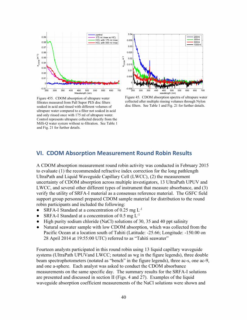
40

VI. CDOM Absorption Measurement Round Robin Results A CDOM absorption measurement round robin activity was conducted in February 2015 to evaluate (1) the recommended refractive index correction for the long pathlength UltraPath and Liquid Waveguide Capillary Cell (LWCC), (2) the measurement uncertainty of CDOM absorption across multiple investigators, 13 UltraPath UPUV and LWCC, and several other different types of instrument that measure absorbance, and (3) verify the utility of SRFA-I material as a consensus reference material. The GSFC field support group personnel prepared CDOM sample material for distribution to the round robin participants and included the following: SRFA-I Standard at a concentration of 0.25 mg L-1 SRFA-I Standard at a concentration of 0.5 mg L-1 High purity sodium chloride (NaCl) solutions of 30, 35 and 40 ppt salinity Natural seawater sample with low CDOM absorption, which was collected from the

Pacific Ocean at a location south of Tahiti (Latitude: -25.66; Longitude: -150.00 on 28 April 2014 at 19:55:00 UTC) referred to as “Tahiti seawater”

Fourteen analysts participated in this round robin using 13 liquid capillary waveguide systems (UltraPath UPUVand LWCC; notated as wg in the figure legends), three double beam spectrophotometers (notated as “bench” in the figure legends), three ac-s, one ac-9, and one a-sphere. Each analyst was asked to conduct the CDOM absorbance measurements on the same specific day. The summary results for the SRFA-I solutions are presented and discussed in section II (Figs. 4 and 27). Examples of the liquid waveguide absorption coefficient measurements of the NaCl solutions were shown and

Figure 455. CDOM absorption of ultrapure water filtrates measured from Pall Supor PES disc filters soaked in acid and rinsed with different volumes of ultrapure water compared to a filter not soaked in acid and only rinsed once with 175 ml of ultrapure water. Control represents ultrapure collected directly from the Milli-Q water system without re-filtration. See Table 1 and Fig. 21 for further details.

Figure 45. CDOM absorption spectra of ultrapure water collected after multiple rinsing volumes through Nylon disc filters. See Table 1 and Fig. 21 for further details.

41

described (Figs. 8-12). The CDOM absorption spectra of the Tahiti seawater computed for the various instruments with the interpolated refractive index correction described previously shows greater variability (Fig. 28) than observed for the SRFA-I materials (Fig. 27). The root mean square error (RMSE) computed from the mean of all the measurements (one a-sphere, three benchtop double beam spectrophotometers, and 11 UltraPath) after removal of outlier spectra ranged from 0 to 0.01 m-1. The RMSE for visible wavelengths was <0.003 m-1 with exception of one UltraPath and the a-sphere (Fig. 28). The RMSE increases in the UV for many of the instruments. Figure 29 shows the Tahiti seawater measurements from different ac instruments in comparison to the overall mean among all instruments. Figure 30 includes the standard deviation of the scans averaged to produce the absorption spectra for each instrument. The uncertainty when measuring absorption at this low range on ac meters is quite high and should be taken into consideration when making field measurements. The importance of producing consistent and multiple ultrapure water calibrations for data processing becomes very apparent when working with these types of water. The measurements of the SRFA-I 0.25 mg L-1 from the ac instruments were in closer agreement to each other and the overall mean than to the Tahiti seawater. This was most likely due to the much higher CDOM (stronger signal) in SRFA-I than that for the Tahiti seawater.

Figure 46. (a) CDOM absorption coefficient spectra of 0.25 mg L-1 SRFA-I solution analyzed on 12 UltraPath UPUV and LWCC instruments, 3 double beam spectrophotometers, one a-sphere, one ac-9 and two ac-s from a multi-investigator round robin conducted in February 2015. (b) CDOM absorption coefficient spectra of 0.50 mg L-1 SRFA-I solution measured on the same instruments on the same day with an additional ac-s. Inset plots present the aCDOM values on a log-scaled axis.

42

Figure 2850. Mean absolute percent error and root mean square error (RMSE) of Tahiti water sample with respect to the mean of all instruments shown in Figure 20. The ac-s instrument shown in Fig. 20 was not included in this analysis.

Figure 48. CDOM absorption spectra of Tahiti Water measured on various ac-s and ac-9 meters compared to the overall Round Robin group average and 1 standard deviation. Note the ac instrument analysis was conducted 2 months after the initial round robin.

Figure 30. CDOM absorption spectra of Tahiti Water measured on various ac-s and ac-9 meters depicting the first standard deviation (sd) of replicate scans compared to the overall Round Robin group average.

Figure 52. SRFA-I 0.25 mg L-1 measured on various ac-s and ac-9 meters compared to the overall Round Robin group average.

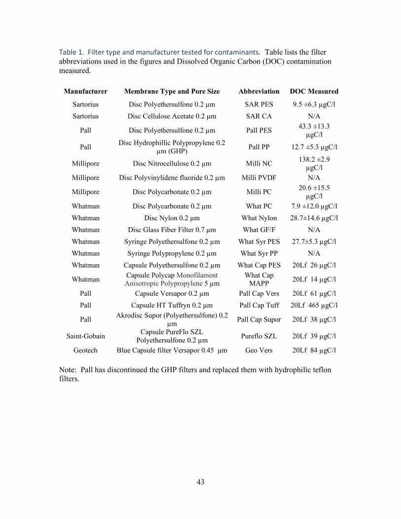
43

Table 1. Filter type and manufacturer tested for contaminants. Table lists the filter abbreviations used in the figures and Dissolved Organic Carbon (DOC) contamination measured.

Manufacturer Membrane Type and Pore Size Abbreviation DOC Measured

Sartorius Disc Polyethersulfone 0.2 µm SAR PES 9.5 ±6.3 µgC/l Sartorius Disc Cellulose Acetate 0.2 µm SAR CA N/A

Pall Disc Polyethersulfone 0.2 µm Pall PES 43.3 ±13.3 µgC/l

Pall Disc Hydrophillic Polypropylene 0.2 µm (GHP) Pall PP 12.7 ±5.3 µgC/l

Millipore Disc Nitrocellulose 0.2 µm Milli NC 138.2 ±2.9 µgC/l

Millipore Disc Polyvinylidene fluoride 0.2 µm Milli PVDF N/A

Millipore Disc Polycarbonate 0.2 µm Milli PC 20.6 ±15.5 µgC/l

Whatman Disc Polycarbonate 0.2 µm What PC 7.9 ±12.0 µgC/l Whatman Disc Nylon 0.2 µm What Nylon 28.7±14.6 µgC/l Whatman Disc Glass Fiber Filter 0.7 µm What GF/F N/A Whatman Syringe Polyethersulfone 0.2 µm What Syr PES 27.7±5.3 µgC/l Whatman Syringe Polypropylene 0.2 µm What Syr PP N/A Whatman Capsule Polyethersulfone 0.2 µm What Cap PES 20Lf 26 µgC/l

Whatman Capsule Polycap Monofilament Anisotropic Polypropylene 5 µm

What Cap MAPP 20Lf 14 µgC/l

Pall Capsule Versapor 0.2 µm Pall Cap Vers 20Lf 61 µgC/l Pall Capsule HT Tuffryn 0.2 µm Pall Cap Tuff 20Lf 465 µgC/l

Pall Akrodisc Supor (Polyethersulfone) 0.2 µm Pall Cap Supor 20Lf 38 µgC/l

Saint-Gobain Capsule PureFlo SZL Polyethersulfone 0.2 µm Pureflo SZL 20Lf 39 µgC/l

Geotech Blue Capsule filter Versapor 0.45 µm Geo Vers 20Lf 84 µgC/l Note: Pall has discontinued the GHP filters and replaced them with hydrophilic teflon filters.

44

Table 2. CDOM absorbance Round Robin participants and the instrumentation used in the comparison.

Researcher Institution Instruments Pathlength Slope Mathias Belz WPI Germany GmbH,

Friedberg, Germany two UltraPath UPUV 1.10 m,

1.82 m negative positive

Jean-Francois Berthon

European Commission, Joint Research Center (JRC), Ispra (Va), Italy

UltraPath UPUV 2.01 m negative

Annick Bricaud Laboratoire d'Océanographie de Villefranche (LOV), France

UltraPath UPUV 2.00 m negative

Emmanuel Boss

University of Maine Orono, ME, USA

acs and ac9 0.25 m N/A

Joaquin Chaves NASA Goddard Space Flight Center Greenbelt, MD, USA

UltraPath UPUV 2.02 m negative

Rosanna Del Vecchio

Earth System Science Interdisciplinary Center University of Maryland College Park, MD, USA

UltraPath UPUV Double Beam Spectrophotometer Shimadzu/UVPC 2401

2.08 m 0.1 m

positive

Eurico D’Sa Department of Oceanography and Coastal Sciences, Louisiana State University, Baton Rouge, LA, USA

UltraPath UPUV PerkinElmer Lambda 850 Double Beam Spectrophotometer

1.98 m 0.1 m

Positive N/A

Scott Freeman NASA Goddard Space Flight Center Greenbelt, MD, USA

ac-s ac-9

0.25 m 0.25 m

N/A

Atsushi Matsuoka

Departement d biologie Univertsite Laval, Quebec, Canada

UltraPath UPUV 1.91 m Negative

Richard Miller Department of Geological Sciences and the Institute for Coastal Sciences and Policy East Carolina University Greenville, NC, USA

UltraPath UPUV Double Beam Spectrophotometer Perkin Elmer Lambda 850

2.06 m 0.1 m

Negative

Norm Nelson Earth Research Center University of California, Santa Barbara, CA, USA

2 UltraPath UPUV 2.02 m 1.94 m

Negative Positive

Aimee Neeley NASA Goddard Space Flight Center Greenbelt, MD, USA

Agilent Cary 4000 Double Beam Spectrophotometer

0.10 m N/A

Michael G. Novak

NASA Goddard Space Flight Center Greenbelt, MD, USA

UltraPath UPUV Cary 100 and 4000 Double Beam Spectrophotometers

1.975 m Negative N/A

Rüdiger Röttgers

Institute for coastal research, Center for Materials and Coastal Research Geesthacht, Germany

LWCC Perkin Elmer Lambda 950 double beam spectrophotometer PSICAM

2.503 m Positive N/A N/A

45

References

Babin, M., D. Stramski, G.M. Ferrari, H., Claustre, A. Bricaud, G. Obolensky, et al., 2003: Variations in the light absorption coefficients of phytoplankton, nonalgal particles and dissolved organic matter in coastal waters around Europe. Journal of Geophysical Research, 108(C7): 3211, http://dx.doi.org/10.1029/2001JC000882.

Belz, M., P. Dress, A. Sukhitskiy, and S. Liu, 1999: Linearity and effective optical pathlength

of liquid waveguide capillary cells. Internal Standardization and Calibration Architectures for Chemical Sensors, 385: 271-282.

Belz, M., K. Larsen, and K.F. Klein, 2006: Fiber optic sample cells for polychromatic

detection of dissolved and particulate matter in natural waters. Advanced Environmental, Chemical, and Biological Sensing Technologies IV, 6377: 63770X.

Birkmann, J., C. Pasel, M. Luckas, and D. Bathen, 2018: UV spectroscopic properties of

principal inorganic ionic species in natural waters. Water Practice and Technology, 13: 879-892.

Blough, N.V. and R. Del Vecchio, 2002: Chromophoric DOM in the coastal environment, in

Biogeochemistry of Marine Dissolved Organic Matter, edited by D.A. Hansell and C.A. Carlson, pp. 509– 546, Academic Press, San Diego, California.

Boss, E., H. Gildor, W. Slade, L. Sokoletsky, A. Oren, and J. Loftin, 2013: Optical properties

of the Dead Sea. Journal of Geophysical Research, 118: 1821-1829. Boss, E., N. Haëntjens, S. Ackleson, B. Balch, A. Chase, G. Dall’Olmo, S. Freeman, Y. Liu,

J. Loftin, W. Neary, N. Nelson, M. Novak, W. Slade, C. Proctor, P. Tortell, and T. Westberry, 2019: Inherent Optical Property Measurements and Protocols: Best practices for the collection and processing of ship-based underway flow-through optical data, IOCCG Ocean Optics and Biogeochemistry Protocols for Satellite Ocean Colour Sensor Validation, Volume 4.0, IOCCG, Dartmouth, NS, Canada.

Cartisano, C.M., R. Del Vecchio, and N.V. Blough, 2018: A calibration/validation protocol

for long/multi-pathlength capillary waveguide spectrometers. Limnology and Oceanography: Methods, 16: 773-786.

D’Sa, E.J., R.G. Steward, A. Vodacek, N.V. Blough, and D. Phinney, 1999: Optical

absorption of seawater colored dissolved organic matter determined using a liquid capillary waveguide. Limnology and Oceanography, 44: 1142-1148.

Fellman, J.B., D.V. D’Amore, and E. Hood, 2008: An evaluation of freezing as a preservation

technique for analyzing dissolved organic C, N and P in surface water samples. Science of the Total Environment, 392: 305–312.

46

Fichot, C.G. and R. Benner, 2012: The spectral slope coefficient of chromophoric dissolved organic matter (S275–295) as a tracer of terrigenous dissolved organic carbon in river-influenced ocean margins. Limnology and Oceanography, 57: 1453–1466, doi:10.4319/lo.2012.57.5.1453.

Floge, S.A., K.R. Hardy, E. Boss, and M.L. Wells, 2009: Analytical intercomparison between

type I and type II long-pathlength liquid core waveguides for the measurement of chromophoric dissolved organic matter. Limnology and Oceanography: Methods, 7(4): 260-268

Fry, E., 2018: Chapter 3: Integrating Cavity Absorption Meters, in Inherent Optical Property

Measurements and Protocols: Absorption Coefficient, edited by A.R. Neeley and A. Mannino, IOCCG Ocean Optics and Biogeochemistry Protocols for Satellite Ocean Colour Sensor Validation, Volume 1.0, IOCCG, Dartmouth, NS, Canada.

Green, S.A. and N.V. Blough, 1994: Optical absorption and fluorescence properties of

chromophoric dissolved organic matter in natural waters. Limnology and Oceanography, 39(8): 1903-1916.

Helms, J.R., A. Stubbins, J.D. Ritchie, E. Minor, D.J. Kieber, and K. Mopper, 2008:

Absorption spectral slopes and slope ratios as indicators of molecular weight, source, and photobleaching of chromophoric dissolved organic matter. Limnology and Oceanography, 53: 955–969.

Hu, C.M., F.E. Muller-Karger, and R.G. Zepp, 2002: Absorbance, absorption coefficient, and

apparent quantum yield: A comment on common ambiguity in the use of these optical concepts. Limnology and Oceanography, 47: 1261−1267.

Johnson, K.S. and L.J. Coletti, 2002: In situ ultraviolet spectrophotometry for high resolution

and long-term monitoring of nitrate, bromide and bisulfide in the ocean. Deep Sea Research Part I, 49: 1291-1305.

Lai, C.Z., M.D. DeGrandpre, B.D. Wasser, T.A. Brandon, D.S. Clucas, E.J. Jaqueth, Z.D.

Benson, C.M. Beatty, and R.S. Spaulding, 2016: Spectrophotometric measurement of freshwater pH with purified meta-cresol purple and phenol red. Limnology and Oceanography: Methods, 14: 864-873.

Lefering, I., R. Röttgers, C. Utschig, and D. McKee, 2017: Uncertainty budgets for liquid

waveguide CDOM absorption measurements. Applied Optics, 56: 6357–6366, doi: 10.1364/AO.56.006357.

Loiselle, S.A., L. Bracchini, A.M. Dattilo, M. Ricci, A. Tognazzi, A. Cózar, and C. Rossi, 2009: The optical characterization of chromophoric dissolved organic matter using wavelength distribution of absorption spectral slopes. Limnology and Oceanography, 54(2), 590-597.

47

Mannino, A., M. Novak, S. Hooker, K. Hyde, and D. Aurin (2014) CDOM Algorithm Development and Validation for the Continental Margin Along the Northeastern U.S. Remote Sensing of Environment, 152: 576-602, doi 10.1016/j.rse.2014.06.027.

Mannino, A., M.E. Russ, and S.B. Hooker, 2008: Algorithm development for satellite-derived

distributions of DOC and CDOM in the U.S. Middle Atlantic Bight. Journal of Geophysical Research, C0705, doi:10.1029/2007JC004493.

Matsuoka, A., E. Boss, M. Babin, L. Karp-Boss, M. Hafez, A. Chekalyuk, C.W. Proctor, P.J.

Werdell, and A. Bricaud, 2017: Pan-Arctic optical characteristics of colored dissolved organic matter: Tracing dissolved organic carbon in changing Arctic waters using satellite ocean color data. Remote Sensing of Environment, 200: 89-101.

Miller, R.L., M. Belz, C. Del Castillo, and R. Trzaska, 2002: Determining CDOM absorption

spectra in diverse coastal environments using a multiple pathlength, liquid core waveguide system. Continental Shelf Research, 22: 1301-1310.

Mitchell, B.G, M. Kahru, J. Wieland, and M. Stramska, 2002: Chapter 15 Determination of

spectral absorption coefficients of particles, dissolved material and phytoplankton for discrete water samples, in Ocean Optics Protocols for Satellite Ocean Color Senor Validation, NASA/TM-2002-210004/Rev3-Vol2, edited by J.L. Mueller and G.S. Fargion, pp. 231-253. NASA Goddard Space Flight Center, Greenbelt, Maryland.

Mitchell, B.G, A. Bricaud, K. Carder, J. Cleveland, G. Ferrari, R. Gould, M. Kahru, M.

Kishino, H. Maske, T. Moisan, L. Moore, N. Nelson, D. Phinney, R. Reynolds, H. Sosik, D. Stramski, S. Tassan, C.C. Trees, A. Weidemann, J. Wieland, and A. Vodacek, 2000: Chapter 12: Determination of spectral absorption coefficients of particles, dissolved material and phytoplankton for discrete water samples, in Ocean Optics Protocols for Satellite Ocean Color Sensor Validation, Revision 2, NASA/TM-2000-209966, edited by G.S. Fargion and J.L. Mueller, pp. 125-153, NASA Goddard Space Flight Center, Greenbelt, Maryland.

Mitchell, B.G., M. Kahru, J. Wieland, and M. Stramska, 2003: Chapter 4 Determination of

spectral absorption coefficients of particles, dissolved material and phytoplankton for discrete water samples, in Ocean Optics Protocols For Satellite Ocean Color Sensor Validation, Revision 4, Volume IV: Inherent Optical Properties: Instruments, Characterizations, Field Measurements and Data Analysis Protocols, NASA/TM-2003-211621/Rev4-Vol.IV, edited by J.L. Mueller, G.S. Fargion, and C.R. McClain, pp. 39-64, NASA Goddard Space Flight Center, Greenbelt, MD 20771.

Nelson, N.B., D.A. Siegel, C.A. Carlson, and C.M. Swan, 2010: Tracing global

biogeochemical cycles and meridional overturning circulation using chromophoric dissolved organic matter. Geophysical Research. Letters, 37: L03610, doi: 10.1029/2009GL042325.

48

Nelson, N.B., D.A. Siegel, C.A. Carlson, C.Swan, W.M. Smethie Jr., and S. Khatiwala, 2007: Hydrography of chromophoric dissolved organic matter in the North Atlantic. Deep Sea Research I, 54: 710–731, doi: 10.1016/j.dsr.2007.02.006.

Obernosterer, I., P. Catala, R. Lami, J. Caparros, J. Ras, A. Bricaud, C. Dupuy, F. van

Wambeke, and P. Lebaron, 2008: Biochemical characteristics and bacterial community structure of the sea surface microlayer in the South Pacific Ocean. Biogeosciences, 5: 693–705.

Pegau, W.S., J.S. Cleveland, W. Doss, C.D. Kennedy, R.A. Maffione, J.L. Mueller, R.

Stone, C.C. Trees, A.D. Weidemann, W. Wells, et al., 1995: A comparison of methods for measurement of the absorption coefficient in natural waters. Journal of Geophysical Research, 100: 13,201-13,220.

Pegau, W.S., D. Gray, and J.R.V. Zaneveld, 1997: Absorption and attenuation of visible and

near-infrared light in water: dependence on temperature and salinity. Applied Optics, 36: 6035-6046.

Röttgers, R., 2018: Chapter 4: Point-Source Integrating Cavity Absorption Meters, in Inherent

Optical Property Measurements and Protocols: Absorption Coefficient, edited by A.R. Neeley and and A. Mannino, IOCCG Ocean Optics and Biogeochemistry Protocols for Satellite Ocean Colour Sensor Validation, Volume 1.0, IOCCG, Dartmouth, NS, Canada.

Sullivan, J., M. Twardowski, J. Zaneveld, C. Moore, A. Barnard, P. Donaghay, and B.

Rhoades, 2006: Hyperspectral temperature and salt dependencies of absorption by water and heavy water in the 400-750 nm spectral range. Applied Optics, 45: 5294-5309.

Tilstone, G.H., R.L. Airs, V.M. Vicente, C. Widdicombe, and C. Llewellyn, 2010: High

concentrations of mycosporine-like amino acids and colored dissolved organic matter in the sea surface microlayer off the Iberian Peninsula. Limnology and Oceanography, 55: 1835-1850.

Twardowski, M.S., E. Boss, J.M. Sullivan, and P.L. Donaghay, 2004: Modeling the spectral

shape of absorption by chromophoric dissolved organic matter. Marine Chemistry, 89: 69-88.

Twardowski, M., S. Freeman, S. Pegau, J.R.V. Zaneveld, J.L. Mueller, and E. Boss, 2018a:

Chapter 2: Reflective Tube Absorption Meters, in Inherent Optical Property Measurements and Protocols: Absorption Coefficient, edited by A.R. Neeley and A. Mannino, IOCCG Ocean Optics and Biogeochemistry Protocols for Satellite Ocean Colour Sensor Validation, Volume 1.0, IOCCG, Dartmouth, NS, Canada.

Twardowski, M., R. Röttgers and D. Stramski, 2018b: Chapter 1: The Absorption Coefficient,

An Overview, in Inherent Optical Property Measurements and Protocols: Absorption Coefficient, edited by A.R. Neeley and A. Mannino, IOCCG Ocean Optics and

49

Biogeochemistry Protocols for Satellite Ocean Colour Sensor Validation, Volume 1.0, IOCCG, Dartmouth, NS, Canada.

Tzortziou M., P. Neale, C. Osburn, P. Megonigal, N. Maie, and R. Jaffé, 2008: Tidal marshes

as a source of optically and chemically distinctive CDOM in the Chesapeake Bay. Limnology and Oceanography, 53: 148-159, doi: 10.4319/lo.2008.53.1.0148.

Weishaar, J.L., G.R. Aiken, B.A. Bergamaschi, M.S. Fram, R. Fujii, and K. Mopper, 2003:

Evaluation of specific ultraviolet absorbance as an indicator of the chemical composition and reactivity of dissolved organic carbon. Environmental science & technology, 37(20): 4702-4708.

Zafiriou, O.C., J. Joussot-Dubien, R.G. Zepp, and R.G. Zika, 1984: Photochemistry of natural

waters. Environmental Science & Technology, 18(12): 358A-371A.

50

Appendix A: WPI Advanced Flowcell Cleaning

World Precision Instruments Alexander Dickson

Product Manager – Muscle Physiology Chemist – Application Research, Optics

175 Sarasota Center Blvd. Sarasota, FL-34240

Tel.: (941) 371 1003 Fax: (941) 377 5428

www.wpiinc.com 08/14/2013

Advanced Flowcell Cleaning Purpose of Document: The purpose of this document is to describe a new cleaning procedure for aggressive cleaning of WPI flowcells. This includes LWCC units, as well as UltraPath flowcells. Preparation of Chemicals: All chemical reagents should be of at least ACS-Grade, preferably HPLC-Grade. This procedure involves the use of caustic and flammable reagents. Consult the manufacturer’s MSDS for necessary safety precautions. Cleaning Solution #1: 0.5M Potassium Hydroxide in 100% Ethanol (briefly, 7.013g KOH in 250mL EtOH). After thorough mixing, the solution should be filtered through a 20µm pore size filter. Cleaning Solution #2: 100% Methanol. Cleaning Solution #3: Ultrapure water, Type I per ASTM D1193-99 or equivalent. Note: Grade 1 ultrapure water per ISO 3696 differs significantly from the above classification. Cleaning Procedure: The preferred method of cleaning involves the use of a spectrophotometer in “monitor mode” throughout the entire cleaning process. This allows the technician to observe the extent of performance improvement as a function of time.

51

The simplest cleaning method involves using a peristaltic pump to flow each cleaning solution through the sample cell in numerical order. It is recommended the pump is configured to “pull” through the cell to avoid possible contamination from degraded peristaltic pump tubing. Each solution is cycled for approximately 3-4 minutes, with a bolus of air introduced between each solution. This procedure is repeated until there is no noticeable improvement in sample cell performance. The flow direction can be reversed between cycles to ensure thorough cleaning. To lessen the time required for the above cleaning method, large bubbles of air can be introduced into the sample cell alternately with the cleaning solutions. This method uses a laminar flow profile and radial diffusion to effectively “scrub” the inside of the sample cell. It is imperative that Solution #2 immediately follow Solution #1 to remove residue remaining on the optical components. Failure to do so will result in poor flowcell performance. Another possible cleaning method involves the use of two syringes of appropriate volume connected to the liquid ports of the sample cell. In numerical order, each cleaning solution is introduced into the sample cell and flushed back and forth between the syringes 10-12 times. This procedure is repeated until there is no noticeable improvement in sample cell performance. Final Rinsing Procedure: Once the technician identifies the point where subsequent cleaning cycles no longer improve the performance of the flowcell, the unit should be flushed with ultrapure water for a period of at least 15 minutes to ensure all cleaning solutions have been completely removed and there are no persistent residues that might affect flowcell performance or stability.

52

Appendix B: Consensus CDOM absorption coefficient values of Suwannee River Fulvic Acid I (SRFA-I) solutions. Table B1. CDOM absorption coefficient values for SRFA-I 0.25 mg L-1 solution from the February 2015 Round Robin mean, median and 2.5% and 97.5% quantile values.

wavelength (nm) mean median 2.5% Quantile 97.5% Quantile 250 1.2343 1.2340 1.1860 1.2949 251 1.2204 1.2189 1.1729 1.2804 252 1.2074 1.2079 1.1614 1.2599 253 1.1934 1.1927 1.1513 1.2459 254 1.1830 1.1810 1.1420 1.2387 255 1.1704 1.1675 1.1313 1.2256 256 1.1575 1.1566 1.1189 1.2075 257 1.1438 1.1436 1.1085 1.1889 258 1.1315 1.1308 1.0976 1.1729 259 1.1185 1.1169 1.0880 1.1560 260 1.1058 1.1036 1.0761 1.1422 261 1.0938 1.0927 1.0667 1.1264 262 1.0798 1.0783 1.0541 1.1093 263 1.0671 1.0660 1.0420 1.0931 264 1.0542 1.0524 1.0317 1.0738 265 1.0410 1.0387 1.0197 1.0617 266 1.0280 1.0254 1.0082 1.0450 267 1.0146 1.0129 0.9948 1.0329 268 1.0014 0.9988 0.9838 1.0161 269 0.9888 0.9869 0.9701 1.0043 270 0.9759 0.9735 0.9598 0.9899 271 0.9629 0.9601 0.9472 0.9780 272 0.9506 0.9485 0.9356 0.9647 273 0.9385 0.9355 0.9235 0.9548 274 0.9266 0.9243 0.9127 0.9405 275 0.9147 0.9130 0.9002 0.9291 276 0.9022 0.9001 0.8884 0.9155 277 0.8907 0.8886 0.8779 0.9049 278 0.8779 0.8753 0.8669 0.8922 279 0.8666 0.8636 0.8539 0.8814 280 0.8541 0.8514 0.8414 0.8695 281 0.8434 0.8413 0.8320 0.8575 282 0.8329 0.8314 0.8220 0.8446 283 0.8218 0.8200 0.8106 0.8354

53

284 0.8094 0.8080 0.7984 0.8225 285 0.7991 0.7980 0.7880 0.8115 286 0.7882 0.7854 0.7786 0.8025 287 0.7767 0.7748 0.7677 0.7917 288 0.7668 0.7650 0.7570 0.7802 289 0.7553 0.7532 0.7469 0.7682 290 0.7447 0.7435 0.7362 0.7577 291 0.7344 0.7322 0.7268 0.7476 292 0.7241 0.7232 0.7152 0.7358 293 0.7136 0.7129 0.7047 0.7255 294 0.7030 0.7016 0.6961 0.7145 295 0.6938 0.6925 0.6851 0.7053 296 0.6839 0.6835 0.6761 0.6950 297 0.6749 0.6744 0.6677 0.6868 298 0.6650 0.6648 0.6568 0.6758 299 0.6546 0.6530 0.6478 0.6665 300 0.6513 0.6502 0.6191 0.6874 301 0.6412 0.6385 0.6100 0.6762 302 0.6318 0.6285 0.6010 0.6652 303 0.6219 0.6192 0.5920 0.6545 304 0.6126 0.6111 0.5833 0.6442 305 0.6035 0.6024 0.5747 0.6340 306 0.5943 0.5938 0.5663 0.6240 307 0.5849 0.5824 0.5576 0.6142 308 0.5763 0.5747 0.5489 0.6047 309 0.5678 0.5664 0.5403 0.5955 310 0.5588 0.5556 0.5320 0.5865 311 0.5508 0.5479 0.5240 0.5776 312 0.5423 0.5393 0.5160 0.5689 313 0.5345 0.5327 0.5082 0.5603 314 0.5264 0.5246 0.5007 0.5519 315 0.5187 0.5165 0.4933 0.5437 316 0.5103 0.5086 0.4862 0.5357 317 0.5033 0.5009 0.4791 0.5279 318 0.4959 0.4941 0.4723 0.5203 319 0.4889 0.4875 0.4656 0.5130 320 0.4818 0.4804 0.4591 0.5059 321 0.4748 0.4733 0.4526 0.4989 322 0.4679 0.4659 0.4462 0.4918 323 0.4610 0.4582 0.4401 0.4847 324 0.4542 0.4523 0.4342 0.4778 325 0.4476 0.4442 0.4282 0.4709 326 0.4417 0.4395 0.4222 0.4643

54

327 0.4350 0.4331 0.4164 0.4577 328 0.4285 0.4257 0.4107 0.4512 329 0.4224 0.4209 0.4051 0.4447 330 0.4161 0.4135 0.3993 0.4383 331 0.4102 0.4081 0.3935 0.4321 332 0.4040 0.4013 0.3880 0.4258 333 0.3977 0.3962 0.3825 0.4195 334 0.3920 0.3907 0.3768 0.4132 335 0.3861 0.3845 0.3711 0.4069 336 0.3803 0.3781 0.3656 0.4012 337 0.3741 0.3713 0.3601 0.3963 338 0.3688 0.3667 0.3547 0.3909 339 0.3628 0.3604 0.3493 0.3845 340 0.3578 0.3552 0.3440 0.3778 341 0.3522 0.3503 0.3388 0.3718 342 0.3474 0.3456 0.3336 0.3662 343 0.3416 0.3389 0.3283 0.3606 344 0.3359 0.3332 0.3231 0.3550 345 0.3306 0.3291 0.3179 0.3495 346 0.3253 0.3230 0.3127 0.3440 347 0.3202 0.3187 0.3077 0.3385 348 0.3147 0.3114 0.3026 0.3332 349 0.3105 0.3085 0.2974 0.3278 350 0.3053 0.3035 0.2922 0.3225 351 0.3002 0.2984 0.2872 0.3172 352 0.2951 0.2934 0.2823 0.3120 353 0.2900 0.2882 0.2774 0.3067 354 0.2849 0.2829 0.2725 0.3015 355 0.2799 0.2779 0.2677 0.2963 356 0.2750 0.2730 0.2630 0.2912 357 0.2702 0.2682 0.2582 0.2862 358 0.2653 0.2635 0.2536 0.2813 359 0.2606 0.2588 0.2489 0.2764 360 0.2558 0.2540 0.2444 0.2716 361 0.2512 0.2492 0.2398 0.2669 362 0.2466 0.2447 0.2353 0.2621 363 0.2420 0.2401 0.2308 0.2572 364 0.2375 0.2358 0.2267 0.2526 365 0.2331 0.2314 0.2225 0.2481 366 0.2288 0.2271 0.2184 0.2437 367 0.2245 0.2227 0.2143 0.2393 368 0.2202 0.2184 0.2102 0.2349 369 0.2161 0.2140 0.2063 0.2307

55

370 0.2119 0.2098 0.2023 0.2265 371 0.2078 0.2057 0.1983 0.2223 372 0.2037 0.2017 0.1944 0.2181 373 0.1997 0.1977 0.1905 0.2140 374 0.1957 0.1937 0.1867 0.2100 375 0.1918 0.1896 0.1830 0.2060 376 0.1880 0.1856 0.1794 0.2019 377 0.1843 0.1821 0.1758 0.1981 378 0.1807 0.1786 0.1722 0.1944 379 0.1771 0.1750 0.1688 0.1907 380 0.1736 0.1714 0.1655 0.1869 381 0.1701 0.1682 0.1623 0.1833 382 0.1668 0.1650 0.1591 0.1798 383 0.1635 0.1615 0.1558 0.1764 384 0.1602 0.1581 0.1526 0.1730 385 0.1569 0.1548 0.1495 0.1695 386 0.1538 0.1517 0.1464 0.1661 387 0.1507 0.1487 0.1435 0.1628 388 0.1476 0.1458 0.1405 0.1597 389 0.1447 0.1429 0.1376 0.1566 390 0.1417 0.1400 0.1346 0.1534 391 0.1388 0.1372 0.1318 0.1504 392 0.1360 0.1345 0.1290 0.1476 393 0.1333 0.1319 0.1263 0.1450 394 0.1306 0.1293 0.1235 0.1422 395 0.1280 0.1268 0.1210 0.1393 396 0.1254 0.1243 0.1186 0.1365 397 0.1229 0.1220 0.1161 0.1338 398 0.1205 0.1196 0.1137 0.1313 399 0.1181 0.1173 0.1114 0.1289 400 0.1158 0.1150 0.1092 0.1265 401 0.1135 0.1128 0.1070 0.1240 402 0.1111 0.1104 0.1047 0.1215 403 0.1090 0.1082 0.1025 0.1192 404 0.1069 0.1061 0.1004 0.1170 405 0.1050 0.1047 0.0984 0.1148 406 0.1029 0.1027 0.0964 0.1127 407 0.1008 0.1004 0.0945 0.1106 408 0.0990 0.0987 0.0926 0.1086 409 0.0970 0.0966 0.0907 0.1065 410 0.0954 0.0947 0.0888 0.1045 411 0.0933 0.0929 0.0870 0.1026 412 0.0917 0.0910 0.0853 0.1008

56

413 0.0898 0.0891 0.0836 0.0990 414 0.0881 0.0873 0.0821 0.0972 415 0.0865 0.0857 0.0805 0.0953 416 0.0848 0.0841 0.0789 0.0935 417 0.0832 0.0825 0.0773 0.0918 418 0.0817 0.0809 0.0757 0.0902 419 0.0799 0.0789 0.0741 0.0886 420 0.0785 0.0773 0.0726 0.0869 421 0.0772 0.0766 0.0712 0.0853 422 0.0756 0.0750 0.0699 0.0839 423 0.0743 0.0739 0.0685 0.0826 424 0.0729 0.0724 0.0671 0.0812 425 0.0717 0.0712 0.0658 0.0798 426 0.0704 0.0699 0.0645 0.0784 427 0.0691 0.0687 0.0632 0.0771 428 0.0678 0.0674 0.0619 0.0757 429 0.0666 0.0662 0.0606 0.0745 430 0.0653 0.0650 0.0595 0.0732 431 0.0642 0.0637 0.0583 0.0720 432 0.0631 0.0625 0.0571 0.0709 433 0.0619 0.0612 0.0560 0.0698 434 0.0608 0.0598 0.0548 0.0686 435 0.0596 0.0589 0.0537 0.0674 436 0.0586 0.0579 0.0526 0.0662 437 0.0575 0.0561 0.0516 0.0650 438 0.0562 0.0551 0.0506 0.0638 439 0.0553 0.0541 0.0496 0.0627 440 0.0544 0.0535 0.0486 0.0617 441 0.0536 0.0526 0.0477 0.0608 442 0.0530 0.0516 0.0468 0.0600 443 0.0521 0.0507 0.0460 0.0591 444 0.0512 0.0497 0.0451 0.0582 445 0.0502 0.0489 0.0442 0.0574 446 0.0493 0.0480 0.0433 0.0565 447 0.0485 0.0473 0.0425 0.0556 448 0.0477 0.0465 0.0417 0.0547 449 0.0469 0.0456 0.0409 0.0539 450 0.0460 0.0449 0.0402 0.0531 451 0.0452 0.0441 0.0394 0.0523 452 0.0445 0.0434 0.0387 0.0514 453 0.0438 0.0426 0.0380 0.0505 454 0.0430 0.0419 0.0373 0.0496 455 0.0424 0.0412 0.0366 0.0487

57

456 0.0416 0.0405 0.0359 0.0479 457 0.0409 0.0398 0.0352 0.0472 458 0.0403 0.0392 0.0346 0.0466 459 0.0396 0.0386 0.0340 0.0460 460 0.0390 0.0380 0.0333 0.0453 461 0.0384 0.0374 0.0327 0.0445 462 0.0376 0.0367 0.0320 0.0438 463 0.0371 0.0362 0.0313 0.0431 464 0.0365 0.0356 0.0307 0.0424 465 0.0360 0.0351 0.0302 0.0418 466 0.0355 0.0345 0.0296 0.0412 467 0.0349 0.0339 0.0290 0.0405 468 0.0341 0.0334 0.0285 0.0398 469 0.0337 0.0329 0.0280 0.0390 470 0.0331 0.0324 0.0274 0.0382 471 0.0325 0.0319 0.0268 0.0374 472 0.0321 0.0313 0.0264 0.0368 473 0.0315 0.0308 0.0259 0.0363 474 0.0310 0.0303 0.0254 0.0358 475 0.0305 0.0299 0.0249 0.0355 476 0.0300 0.0296 0.0245 0.0350 477 0.0295 0.0292 0.0241 0.0343 478 0.0291 0.0288 0.0238 0.0338 479 0.0285 0.0278 0.0233 0.0333 480 0.0281 0.0279 0.0229 0.0330 481 0.0275 0.0270 0.0224 0.0326 482 0.0271 0.0269 0.0221 0.0323 483 0.0266 0.0261 0.0220 0.0320 484 0.0264 0.0262 0.0218 0.0317 485 0.0257 0.0250 0.0205 0.0316 486 0.0255 0.0248 0.0210 0.0314 487 0.0254 0.0250 0.0208 0.0312 488 0.0250 0.0247 0.0204 0.0308 489 0.0247 0.0245 0.0199 0.0301 490 0.0244 0.0235 0.0194 0.0292 491 0.0241 0.0237 0.0188 0.0285 492 0.0237 0.0233 0.0184 0.0279 493 0.0233 0.0226 0.0180 0.0282 494 0.0229 0.0222 0.0176 0.0272 495 0.0227 0.0222 0.0172 0.0272 496 0.0224 0.0217 0.0169 0.0273 497 0.0221 0.0216 0.0166 0.0272 498 0.0217 0.0210 0.0163 0.0268

58

499 0.0213 0.0206 0.0160 0.0252 500 0.0210 0.0204 0.0158 0.0250 501 0.0208 0.0201 0.0155 0.0257 502 0.0204 0.0198 0.0152 0.0246 503 0.0202 0.0197 0.0150 0.0251 504 0.0199 0.0191 0.0148 0.0255 505 0.0194 0.0188 0.0146 0.0234 506 0.0191 0.0185 0.0143 0.0231 507 0.0188 0.0186 0.0140 0.0228 508 0.0185 0.0183 0.0137 0.0224 509 0.0180 0.0176 0.0134 0.0221 510 0.0177 0.0173 0.0132 0.0218 511 0.0174 0.0170 0.0129 0.0216 512 0.0172 0.0171 0.0127 0.0214 513 0.0169 0.0166 0.0125 0.0212 514 0.0166 0.0163 0.0122 0.0208 515 0.0163 0.0158 0.0120 0.0205 516 0.0160 0.0158 0.0118 0.0203 517 0.0158 0.0155 0.0116 0.0201 518 0.0156 0.0152 0.0113 0.0199 519 0.0153 0.0149 0.0111 0.0196 520 0.0151 0.0146 0.0109 0.0194 521 0.0148 0.0145 0.0107 0.0192 522 0.0147 0.0146 0.0104 0.0190 523 0.0144 0.0142 0.0102 0.0188 524 0.0140 0.0139 0.0101 0.0185 525 0.0140 0.0136 0.0100 0.0183 526 0.0138 0.0134 0.0098 0.0181 527 0.0136 0.0133 0.0096 0.0178 528 0.0134 0.0132 0.0093 0.0176 529 0.0132 0.0129 0.0091 0.0174 530 0.0130 0.0127 0.0090 0.0173 531 0.0128 0.0125 0.0089 0.0171 532 0.0127 0.0124 0.0087 0.0169 533 0.0124 0.0122 0.0086 0.0166 534 0.0123 0.0122 0.0084 0.0164 535 0.0122 0.0120 0.0082 0.0162 536 0.0118 0.0111 0.0081 0.0160 537 0.0117 0.0116 0.0080 0.0158 538 0.0115 0.0113 0.0078 0.0156 539 0.0114 0.0112 0.0077 0.0154 540 0.0111 0.0106 0.0075 0.0153 541 0.0111 0.0109 0.0073 0.0151

59

542 0.0109 0.0106 0.0071 0.0149 543 0.0106 0.0101 0.0070 0.0147 544 0.0106 0.0104 0.0068 0.0145 545 0.0104 0.0098 0.0067 0.0144 546 0.0103 0.0100 0.0066 0.0143 547 0.0099 0.0095 0.0064 0.0140 548 0.0098 0.0096 0.0063 0.0138 549 0.0098 0.0093 0.0063 0.0136 550 0.0095 0.0089 0.0061 0.0135 551 0.0095 0.0089 0.0060 0.0135 552 0.0093 0.0087 0.0058 0.0134 553 0.0092 0.0086 0.0057 0.0132 554 0.0090 0.0084 0.0055 0.0131 555 0.0089 0.0085 0.0055 0.0129 556 0.0088 0.0086 0.0053 0.0128 557 0.0085 0.0080 0.0052 0.0127 558 0.0084 0.0079 0.0051 0.0126 559 0.0083 0.0077 0.0051 0.0124 560 0.0082 0.0077 0.0051 0.0124 561 0.0081 0.0075 0.0050 0.0123 562 0.0080 0.0077 0.0050 0.0123 563 0.0078 0.0072 0.0049 0.0123 564 0.0077 0.0071 0.0048 0.0123 565 0.0076 0.0070 0.0047 0.0123 566 0.0075 0.0069 0.0046 0.0124 567 0.0074 0.0068 0.0046 0.0126 568 0.0074 0.0067 0.0046 0.0126 569 0.0072 0.0066 0.0046 0.0125 570 0.0072 0.0065 0.0045 0.0126 571 0.0071 0.0064 0.0044 0.0127 572 0.0071 0.0063 0.0045 0.0127 573 0.0069 0.0063 0.0043 0.0126 574 0.0066 0.0060 0.0035 0.0126 575 0.0067 0.0061 0.0044 0.0126 576 0.0065 0.0057 0.0043 0.0127 577 0.0065 0.0059 0.0037 0.0126 578 0.0064 0.0058 0.0039 0.0125 579 0.0063 0.0056 0.0037 0.0124 580 0.0062 0.0056 0.0035 0.0124 581 0.0061 0.0055 0.0029 0.0124 582 0.0061 0.0054 0.0040 0.0123 583 0.0058 0.0053 0.0027 0.0120 584 0.0057 0.0050 0.0031 0.0118

60

585 0.0057 0.0051 0.0035 0.0117 586 0.0056 0.0050 0.0033 0.0116 587 0.0054 0.0047 0.0032 0.0114 588 0.0055 0.0049 0.0034 0.0112 589 0.0051 0.0045 0.0016 0.0109 590 0.0053 0.0047 0.0031 0.0108 591 0.0050 0.0042 0.0027 0.0107 592 0.0047 0.0042 0.0018 0.0107 593 0.0048 0.0043 0.0025 0.0106 594 0.0047 0.0043 0.0016 0.0104 595 0.0045 0.0038 0.0013 0.0102 596 0.0045 0.0041 0.0017 0.0101 597 0.0043 0.0036 0.0007 0.0100 598 0.0042 0.0035 0.0011 0.0100 599 0.0041 0.0034 0.0016 0.0099 600 0.0040 0.0034 0.0004 0.0097 601 0.0038 0.0032 -0.0003 0.0096 602 0.0036 0.0031 0.0001 0.0095 603 0.0036 0.0030 0.0004 0.0094 604 0.0035 0.0030 -0.0004 0.0093 605 0.0033 0.0029 -0.0004 0.0091 606 0.0034 0.0028 0.0001 0.0089 607 0.0033 0.0027 -0.0003 0.0089 608 0.0033 0.0029 0.0001 0.0088 609 0.0031 0.0026 -0.0001 0.0086 610 0.0031 0.0028 -0.0010 0.0082 611 0.0031 0.0026 0.0002 0.0080 612 0.0029 0.0026 -0.0003 0.0080 613 0.0029 0.0026 -0.0007 0.0078 614 0.0029 0.0025 0.0006 0.0073 615 0.0028 0.0027 0.0001 0.0070 616 0.0028 0.0026 -0.0008 0.0071 617 0.0028 0.0025 -0.0003 0.0071 618 0.0028 0.0025 0.0005 0.0067 619 0.0027 0.0026 0.0004 0.0064 620 0.0026 0.0023 0.0003 0.0064 621 0.0026 0.0024 -0.0001 0.0064 622 0.0025 0.0024 -0.0009 0.0062 623 0.0025 0.0023 0.0001 0.0058 624 0.0025 0.0022 0.0001 0.0055 625 0.0024 0.0023 -0.0008 0.0053 626 0.0023 0.0022 -0.0002 0.0052 627 0.0022 0.0021 0.0003 0.0051

61

628 0.0022 0.0022 -0.0003 0.0049 629 0.0020 0.0020 -0.0001 0.0047 630 0.0021 0.0021 -0.0004 0.0045 631 0.0019 0.0020 -0.0006 0.0044 632 0.0020 0.0020 0.0006 0.0044 633 0.0018 0.0020 -0.0008 0.0044 634 0.0018 0.0020 -0.0002 0.0042 635 0.0018 0.0019 -0.0005 0.0039 636 0.0017 0.0018 -0.0002 0.0038 637 0.0018 0.0019 -0.0003 0.0037 638 0.0017 0.0018 -0.0005 0.0036 639 0.0018 0.0019 -0.0004 0.0034 640 0.0016 0.0018 -0.0004 0.0033 641 0.0017 0.0018 0.0003 0.0032 642 0.0016 0.0017 -0.0002 0.0031 643 0.0017 0.0017 0.0001 0.0029 644 0.0016 0.0016 0.0006 0.0028 645 0.0016 0.0015 0.0006 0.0029 646 0.0014 0.0015 -0.0001 0.0029 647 0.0016 0.0015 0.0006 0.0029 648 0.0017 0.0015 0.0006 0.0031 649 0.0015 0.0013 0.0004 0.0037 650 0.0015 0.0011 0.0000 0.0045 651 0.0016 0.0011 0.0002 0.0052 652 0.0016 0.0011 0.0001 0.0058 653 0.0017 0.0012 0.0001 0.0061 654 0.0016 0.0012 0.0000 0.0063 655 0.0017 0.0011 0.0003 0.0064 656 0.0016 0.0011 -0.0006 0.0064 657 0.0016 0.0010 0.0004 0.0064 658 0.0015 0.0009 -0.0001 0.0063 659 0.0014 0.0009 -0.0002 0.0060 660 0.0013 0.0009 -0.0003 0.0055 661 0.0012 0.0009 -0.0001 0.0047 662 0.0011 0.0008 0.0000 0.0039 663 0.0008 0.0007 -0.0011 0.0032 664 0.0008 0.0007 -0.0003 0.0024 665 0.0007 0.0007 -0.0002 0.0019 666 0.0006 0.0007 -0.0005 0.0016 667 0.0006 0.0006 -0.0005 0.0013 668 0.0005 0.0006 -0.0010 0.0015 669 0.0006 0.0006 -0.0008 0.0016 670 0.0006 0.0005 -0.0007 0.0018

62

671 0.0005 0.0005 -0.0007 0.0017 672 0.0004 0.0005 -0.0013 0.0013 673 0.0004 0.0005 -0.0008 0.0013 674 0.0005 0.0005 -0.0005 0.0015 675 0.0003 0.0005 -0.0009 0.0015 676 0.0006 0.0005 -0.0006 0.0037 677 0.0005 0.0005 -0.0006 0.0013 678 0.0005 0.0005 -0.0009 0.0013 679 0.0001 0.0004 -0.0049 0.0013 680 0.0003 0.0003 -0.0013 0.0013 681 0.0002 0.0003 -0.0017 0.0012 682 0.0002 0.0003 -0.0012 0.0012 683 0.0002 0.0004 -0.0009 0.0010 684 0.0002 0.0003 -0.0011 0.0010 685 0.0002 0.0003 -0.0010 0.0010 686 0.0002 0.0003 -0.0011 0.0013 687 0.0001 0.0003 -0.0014 0.0013 688 0.0001 0.0002 -0.0011 0.0011 689 0.0002 0.0002 -0.0009 0.0010 690 0.0000 0.0002 -0.0019 0.0006 691 0.0001 0.0002 -0.0013 0.0005 692 0.0000 0.0002 -0.0015 0.0006 693 0.0000 0.0001 -0.0014 0.0007 694 -0.0001 0.0001 -0.0018 0.0006 695 -0.0001 0.0000 -0.0020 0.0004 696 -0.0001 0.0001 -0.0016 0.0003 697 -0.0004 0.0000 -0.0022 0.0002 698 -0.0004 -0.0001 -0.0029 0.0000 699 -0.0005 -0.0001 -0.0027 0.0000 700 -0.0006 -0.0001 -0.0027 0.0000

63

Table B2. CDOM absorption coefficient values for SRFA-I 0.50 mg L-1 solution from the February 2015 Round Robin mean, median and 2.5% and 97.5% quantile values.

wavelength (nm)

mean median 2.5% Quantile 97.5% Quantile

250 2.5075 2.4996 2.4620 2.5609 251 2.4855 2.4749 2.4414 2.5402 252 2.4630 2.4518 2.4182 2.5189 253 2.4425 2.4288 2.3996 2.4991 254 2.4216 2.4063 2.3789 2.4798 255 2.4020 2.3851 2.3608 2.4602 256 2.3820 2.3629 2.3404 2.4426 257 2.3616 2.3414 2.3213 2.4222 258 2.3419 2.3209 2.3018 2.4032 259 2.3230 2.2998 2.2846 2.3845 260 2.3036 2.2782 2.2677 2.3649 261 2.2842 2.2567 2.2505 2.3453 262 2.2634 2.2352 2.2284 2.3266 263 2.2413 2.2137 2.2057 2.3044 264 2.2189 2.1910 2.1836 2.2822 265 2.1968 2.1676 2.1616 2.2611 266 2.1738 2.1444 2.1371 2.2399 267 2.1518 2.1209 2.1164 2.2182 268 2.1285 2.0972 2.0928 2.1955 269 2.1046 2.0731 2.0679 2.1728 270 2.0820 2.0494 2.0457 2.1510 271 2.0584 2.0250 2.0230 2.1273 272 2.0355 2.0010 1.9998 2.1058 273 2.0109 1.9776 1.9741 2.0810 274 1.9870 1.9535 1.9515 2.0561 275 1.9634 1.9288 1.9283 2.0331 276 1.9387 1.9042 1.9031 2.0087 277 1.9142 1.8798 1.8791 1.9838 278 1.8875 1.8549 1.8482 1.9593 279 1.8624 1.8306 1.8229 1.9338 280 1.8373 1.8064 1.7974 1.9080 281 1.8135 1.7821 1.7755 1.8829 282 1.7901 1.7586 1.7554 1.8564 283 1.7655 1.7343 1.7313 1.8309 284 1.7408 1.7100 1.7060 1.8065 285 1.7147 1.6865 1.6803 1.7773 286 1.6898 1.6623 1.6559 1.7513 287 1.6652 1.6377 1.6337 1.7240

64

288 1.6402 1.6146 1.6083 1.6976 289 1.6139 1.5908 1.5818 1.6690 290 1.5893 1.5667 1.5588 1.6424 291 1.5647 1.5439 1.5339 1.6164 292 1.5403 1.5205 1.5108 1.5895 293 1.5159 1.4983 1.4874 1.5620 294 1.4914 1.4756 1.4629 1.5357 295 1.4683 1.4530 1.4415 1.5103 296 1.4444 1.4309 1.4193 1.4829 297 1.4194 1.4088 1.3921 1.4572 298 1.3953 1.3872 1.3675 1.4312 299 1.3748 1.3659 1.3528 1.4057 300 1.3100 1.3195 1.2259 1.3809 301 1.2904 1.3001 1.2076 1.3551 302 1.2716 1.2810 1.1898 1.3314 303 1.2531 1.2619 1.1720 1.3091 304 1.2347 1.2435 1.1541 1.2916 305 1.2161 1.2252 1.1366 1.2737 306 1.1979 1.2071 1.1198 1.2552 307 1.1801 1.1892 1.1033 1.2380 308 1.1624 1.1713 1.0869 1.2214 309 1.1452 1.1535 1.0706 1.2047 310 1.1279 1.1361 1.0547 1.1877 311 1.1112 1.1189 1.0392 1.1710 312 1.0946 1.1018 1.0244 1.1548 313 1.0783 1.0847 1.0099 1.1384 314 1.0620 1.0680 0.9956 1.1209 315 1.0460 1.0522 0.9812 1.1035 316 1.0308 1.0364 0.9672 1.0890 317 1.0154 1.0206 0.9536 1.0745 318 1.0005 1.0048 0.9402 1.0582 319 0.9858 0.9902 0.9271 1.0417 320 0.9713 0.9756 0.9142 1.0265 321 0.9571 0.9615 0.9015 1.0117 322 0.9432 0.9475 0.8892 0.9969 323 0.9293 0.9319 0.8772 0.9821 324 0.9160 0.9192 0.8654 0.9676 325 0.9028 0.9041 0.8537 0.9535 326 0.8896 0.8908 0.8419 0.9396 327 0.8766 0.8769 0.8303 0.9262 328 0.8639 0.8637 0.8188 0.9129 329 0.8515 0.8516 0.8075 0.8996 330 0.8389 0.8382 0.7957 0.8864

65

331 0.8268 0.8262 0.7839 0.8734 332 0.8148 0.8142 0.7723 0.8604 333 0.8028 0.8022 0.7607 0.8482 334 0.7909 0.7903 0.7492 0.8360 335 0.7791 0.7785 0.7378 0.8238 336 0.7677 0.7671 0.7269 0.8116 337 0.7561 0.7559 0.7162 0.7993 338 0.7448 0.7446 0.7053 0.7870 339 0.7334 0.7329 0.6944 0.7750 340 0.7221 0.7213 0.6835 0.7635 341 0.7109 0.7101 0.6727 0.7519 342 0.6998 0.6993 0.6620 0.7399 343 0.6890 0.6884 0.6516 0.7280 344 0.6779 0.6773 0.6412 0.7168 345 0.6672 0.6665 0.6309 0.7055 346 0.6563 0.6558 0.6206 0.6945 347 0.6457 0.6452 0.6102 0.6834 348 0.6352 0.6347 0.5998 0.6724 349 0.6237 0.6207 0.5897 0.6613 350 0.6128 0.6107 0.5796 0.6501 351 0.6028 0.6004 0.5696 0.6388 352 0.5922 0.5902 0.5597 0.6281 353 0.5823 0.5799 0.5500 0.6177 354 0.5720 0.5695 0.5403 0.6071 355 0.5618 0.5594 0.5308 0.5963 356 0.5521 0.5496 0.5213 0.5856 357 0.5424 0.5399 0.5119 0.5755 358 0.5326 0.5304 0.5027 0.5654 359 0.5230 0.5209 0.4935 0.5551 360 0.5135 0.5111 0.4844 0.5449 361 0.5040 0.5014 0.4753 0.5350 362 0.4948 0.4938 0.4666 0.5251 363 0.4854 0.4831 0.4579 0.5151 364 0.4762 0.4744 0.4492 0.5052 365 0.4676 0.4656 0.4405 0.4956 366 0.4588 0.4566 0.4323 0.4861 367 0.4498 0.4476 0.4240 0.4767 368 0.4413 0.4389 0.4159 0.4674 369 0.4328 0.4303 0.4077 0.4584 370 0.4246 0.4219 0.3998 0.4500 371 0.4161 0.4137 0.3920 0.4415 372 0.4080 0.4055 0.3842 0.4331 373 0.3998 0.3974 0.3764 0.4248

66

374 0.3919 0.3893 0.3687 0.4167 375 0.3841 0.3812 0.3612 0.4085 376 0.3763 0.3733 0.3538 0.4004 377 0.3688 0.3660 0.3466 0.3927 378 0.3616 0.3587 0.3396 0.3853 379 0.3544 0.3516 0.3327 0.3779 380 0.3472 0.3447 0.3259 0.3704 381 0.3403 0.3381 0.3194 0.3632 382 0.3335 0.3315 0.3128 0.3561 383 0.3265 0.3250 0.3065 0.3491 384 0.3197 0.3186 0.3001 0.3421 385 0.3137 0.3122 0.2938 0.3351 386 0.3072 0.3059 0.2876 0.3284 387 0.3008 0.2998 0.2818 0.3218 388 0.2947 0.2939 0.2761 0.3154 389 0.2888 0.2881 0.2703 0.3091 390 0.2829 0.2824 0.2645 0.3029 391 0.2770 0.2768 0.2589 0.2968 392 0.2714 0.2712 0.2536 0.2910 393 0.2658 0.2658 0.2483 0.2855 394 0.2606 0.2607 0.2433 0.2799 395 0.2554 0.2555 0.2383 0.2743 396 0.2502 0.2504 0.2334 0.2688 397 0.2452 0.2454 0.2286 0.2635 398 0.2404 0.2407 0.2242 0.2584 399 0.2356 0.2360 0.2197 0.2535 400 0.2309 0.2313 0.2154 0.2486 401 0.2262 0.2265 0.2111 0.2436 402 0.2216 0.2223 0.2067 0.2387 403 0.2173 0.2181 0.2022 0.2341 404 0.2130 0.2139 0.1980 0.2296 405 0.2089 0.2096 0.1938 0.2253 406 0.2048 0.2056 0.1900 0.2211 407 0.2008 0.2017 0.1862 0.2170 408 0.1969 0.1978 0.1827 0.2130 409 0.1930 0.1940 0.1793 0.2091 410 0.1894 0.1903 0.1759 0.2052 411 0.1856 0.1865 0.1724 0.2014 412 0.1821 0.1828 0.1690 0.1976 413 0.1785 0.1792 0.1660 0.1939 414 0.1752 0.1757 0.1629 0.1904 415 0.1718 0.1723 0.1596 0.1869 416 0.1685 0.1690 0.1562 0.1834

67

417 0.1653 0.1656 0.1533 0.1800 418 0.1622 0.1622 0.1501 0.1767 419 0.1590 0.1591 0.1472 0.1735 420 0.1560 0.1559 0.1441 0.1704 421 0.1532 0.1530 0.1419 0.1673 422 0.1502 0.1501 0.1387 0.1646 423 0.1476 0.1473 0.1364 0.1620 424 0.1449 0.1445 0.1336 0.1592 425 0.1423 0.1418 0.1317 0.1565 426 0.1397 0.1391 0.1291 0.1538 427 0.1372 0.1365 0.1266 0.1512 428 0.1347 0.1339 0.1241 0.1486 429 0.1323 0.1314 0.1220 0.1461 430 0.1297 0.1289 0.1198 0.1436 431 0.1275 0.1265 0.1174 0.1412 432 0.1252 0.1241 0.1148 0.1390 433 0.1230 0.1217 0.1129 0.1367 434 0.1206 0.1195 0.1106 0.1345 435 0.1185 0.1173 0.1090 0.1321 436 0.1164 0.1150 0.1064 0.1297 437 0.1142 0.1128 0.1054 0.1274 438 0.1118 0.1108 0.1016 0.1252 439 0.1099 0.1087 0.1012 0.1231 440 0.1082 0.1068 0.0991 0.1212 441 0.1066 0.1068 0.0977 0.1193 442 0.1047 0.1045 0.0958 0.1176 443 0.1029 0.1018 0.0941 0.1158 444 0.1013 0.1007 0.0926 0.1140 445 0.0995 0.0986 0.0908 0.1123 446 0.0978 0.0962 0.0891 0.1107 447 0.0962 0.0945 0.0881 0.1089 448 0.0946 0.0929 0.0865 0.1071 449 0.0930 0.0912 0.0847 0.1054 450 0.0913 0.0896 0.0829 0.1038 451 0.0897 0.0881 0.0811 0.1021 452 0.0884 0.0881 0.0801 0.1004 453 0.0868 0.0851 0.0793 0.0986 454 0.0853 0.0836 0.0780 0.0969 455 0.0840 0.0822 0.0767 0.0953 456 0.0826 0.0821 0.0743 0.0939 457 0.0812 0.0799 0.0729 0.0925 458 0.0798 0.0781 0.0723 0.0911 459 0.0786 0.0773 0.0706 0.0897

68

460 0.0774 0.0763 0.0702 0.0884 461 0.0760 0.0743 0.0694 0.0869 462 0.0748 0.0738 0.0673 0.0854 463 0.0737 0.0729 0.0661 0.0839 464 0.0724 0.0706 0.0650 0.0827 465 0.0713 0.0695 0.0644 0.0815 466 0.0703 0.0694 0.0639 0.0802 467 0.0691 0.0673 0.0626 0.0789 468 0.0679 0.0663 0.0613 0.0775 469 0.0669 0.0662 0.0600 0.0761 470 0.0657 0.0648 0.0592 0.0750 471 0.0646 0.0640 0.0573 0.0738 472 0.0636 0.0627 0.0571 0.0727 473 0.0626 0.0624 0.0550 0.0716 474 0.0615 0.0609 0.0546 0.0705 475 0.0605 0.0595 0.0539 0.0695 476 0.0596 0.0590 0.0529 0.0685 477 0.0585 0.0573 0.0521 0.0675 478 0.0577 0.0567 0.0516 0.0664 479 0.0567 0.0554 0.0505 0.0654 480 0.0558 0.0552 0.0489 0.0644 481 0.0548 0.0536 0.0492 0.0634 482 0.0539 0.0527 0.0481 0.0626 483 0.0531 0.0522 0.0475 0.0622 484 0.0523 0.0510 0.0467 0.0618 485 0.0514 0.0503 0.0457 0.0614 486 0.0508 0.0497 0.0450 0.0609 487 0.0504 0.0490 0.0442 0.0603 488 0.0499 0.0495 0.0427 0.0595 489 0.0492 0.0487 0.0423 0.0582 490 0.0484 0.0477 0.0412 0.0567 491 0.0475 0.0468 0.0414 0.0558 492 0.0468 0.0460 0.0409 0.0550 493 0.0460 0.0453 0.0395 0.0541 494 0.0452 0.0448 0.0386 0.0533 495 0.0445 0.0441 0.0390 0.0526 496 0.0438 0.0433 0.0374 0.0519 497 0.0431 0.0425 0.0372 0.0511 498 0.0425 0.0418 0.0363 0.0503 499 0.0418 0.0411 0.0359 0.0496 500 0.0412 0.0405 0.0350 0.0490 501 0.0406 0.0398 0.0347 0.0483 502 0.0399 0.0392 0.0344 0.0475

69

503 0.0393 0.0387 0.0338 0.0469 504 0.0386 0.0380 0.0327 0.0464 505 0.0381 0.0368 0.0327 0.0458 506 0.0375 0.0369 0.0325 0.0452 507 0.0369 0.0358 0.0313 0.0446 508 0.0364 0.0359 0.0311 0.0440 509 0.0357 0.0347 0.0294 0.0434 510 0.0351 0.0342 0.0294 0.0428 511 0.0346 0.0342 0.0295 0.0423 512 0.0341 0.0338 0.0286 0.0417 513 0.0335 0.0326 0.0277 0.0412 514 0.0330 0.0322 0.0276 0.0406 515 0.0324 0.0317 0.0263 0.0400 516 0.0319 0.0311 0.0268 0.0395 517 0.0315 0.0306 0.0270 0.0390 518 0.0309 0.0305 0.0248 0.0384 519 0.0305 0.0299 0.0252 0.0379 520 0.0299 0.0293 0.0244 0.0374 521 0.0294 0.0288 0.0242 0.0370 522 0.0291 0.0286 0.0243 0.0365 523 0.0285 0.0279 0.0233 0.0360 524 0.0280 0.0275 0.0230 0.0355 525 0.0277 0.0271 0.0230 0.0351 526 0.0274 0.0266 0.0223 0.0347 527 0.0269 0.0262 0.0214 0.0342 528 0.0265 0.0258 0.0218 0.0337 529 0.0260 0.0254 0.0208 0.0334 530 0.0256 0.0250 0.0206 0.0330 531 0.0253 0.0246 0.0206 0.0326 532 0.0249 0.0242 0.0193 0.0321 533 0.0245 0.0238 0.0198 0.0317 534 0.0241 0.0235 0.0201 0.0314 535 0.0238 0.0231 0.0194 0.0310 536 0.0234 0.0228 0.0179 0.0306 537 0.0231 0.0223 0.0188 0.0302 538 0.0227 0.0219 0.0171 0.0298 539 0.0224 0.0216 0.0179 0.0294 540 0.0220 0.0212 0.0173 0.0291 541 0.0218 0.0209 0.0170 0.0288 542 0.0213 0.0201 0.0165 0.0284 543 0.0209 0.0202 0.0156 0.0280 544 0.0207 0.0197 0.0165 0.0276 545 0.0204 0.0194 0.0154 0.0273

70

546 0.0201 0.0192 0.0151 0.0269 547 0.0197 0.0187 0.0146 0.0265 548 0.0193 0.0183 0.0145 0.0261 549 0.0191 0.0180 0.0146 0.0258 550 0.0188 0.0177 0.0149 0.0256 551 0.0185 0.0174 0.0138 0.0254 552 0.0182 0.0171 0.0139 0.0252 553 0.0180 0.0168 0.0141 0.0249 554 0.0177 0.0168 0.0133 0.0246 555 0.0175 0.0164 0.0131 0.0243 556 0.0171 0.0160 0.0125 0.0241 557 0.0169 0.0157 0.0134 0.0239 558 0.0165 0.0154 0.0125 0.0237 559 0.0164 0.0152 0.0125 0.0236 560 0.0162 0.0152 0.0117 0.0234 561 0.0159 0.0147 0.0121 0.0232 562 0.0157 0.0144 0.0117 0.0231 563 0.0154 0.0142 0.0110 0.0230 564 0.0152 0.0140 0.0113 0.0231 565 0.0149 0.0138 0.0109 0.0232 566 0.0147 0.0135 0.0103 0.0233 567 0.0145 0.0133 0.0105 0.0235 568 0.0143 0.0131 0.0101 0.0236 569 0.0141 0.0129 0.0096 0.0235 570 0.0140 0.0127 0.0099 0.0236 571 0.0137 0.0125 0.0089 0.0237 572 0.0136 0.0123 0.0092 0.0237 573 0.0133 0.0122 0.0087 0.0236 574 0.0130 0.0120 0.0080 0.0236 575 0.0128 0.0118 0.0079 0.0235 576 0.0127 0.0115 0.0077 0.0235 577 0.0125 0.0114 0.0074 0.0234 578 0.0124 0.0113 0.0078 0.0232 579 0.0121 0.0110 0.0078 0.0230 580 0.0119 0.0108 0.0069 0.0229 581 0.0117 0.0106 0.0075 0.0228 582 0.0117 0.0105 0.0070 0.0226 583 0.0113 0.0103 0.0065 0.0223 584 0.0111 0.0102 0.0064 0.0219 585 0.0110 0.0100 0.0063 0.0216 586 0.0108 0.0098 0.0064 0.0214 587 0.0106 0.0096 0.0058 0.0211 588 0.0104 0.0094 0.0060 0.0207

71

589 0.0101 0.0093 0.0049 0.0203 590 0.0101 0.0090 0.0056 0.0200 591 0.0097 0.0089 0.0049 0.0198 592 0.0096 0.0087 0.0050 0.0196 593 0.0093 0.0084 0.0048 0.0193 594 0.0092 0.0083 0.0053 0.0190 595 0.0089 0.0081 0.0051 0.0187 596 0.0088 0.0079 0.0048 0.0185 597 0.0085 0.0078 0.0051 0.0183 598 0.0084 0.0076 0.0043 0.0181 599 0.0083 0.0074 0.0048 0.0178 600 0.0078 0.0072 0.0042 0.0175 601 0.0077 0.0071 0.0040 0.0173 602 0.0076 0.0069 0.0039 0.0171 603 0.0075 0.0068 0.0041 0.0169 604 0.0073 0.0066 0.0038 0.0165 605 0.0070 0.0064 0.0037 0.0162 606 0.0070 0.0063 0.0037 0.0159 607 0.0067 0.0062 0.0029 0.0157 608 0.0067 0.0061 0.0037 0.0155 609 0.0065 0.0060 0.0027 0.0152 610 0.0063 0.0059 0.0025 0.0148 611 0.0062 0.0058 0.0033 0.0144 612 0.0061 0.0057 0.0024 0.0142 613 0.0060 0.0056 0.0026 0.0138 614 0.0060 0.0055 0.0033 0.0132 615 0.0058 0.0054 0.0029 0.0128 616 0.0056 0.0053 0.0022 0.0127 617 0.0056 0.0051 0.0029 0.0126 618 0.0056 0.0051 0.0026 0.0121 619 0.0055 0.0050 0.0027 0.0116 620 0.0054 0.0049 0.0029 0.0114 621 0.0052 0.0048 0.0022 0.0113 622 0.0051 0.0047 0.0014 0.0109 623 0.0050 0.0046 0.0022 0.0104 624 0.0049 0.0045 0.0020 0.0100 625 0.0047 0.0044 0.0009 0.0098 626 0.0046 0.0044 0.0015 0.0097 627 0.0046 0.0043 0.0018 0.0094 628 0.0045 0.0042 0.0012 0.0090 629 0.0044 0.0041 0.0017 0.0085 630 0.0043 0.0041 0.0020 0.0081 631 0.0042 0.0040 0.0009 0.0079

72

632 0.0042 0.0039 0.0019 0.0078 633 0.0041 0.0038 0.0017 0.0077 634 0.0040 0.0037 0.0010 0.0074 635 0.0038 0.0037 0.0012 0.0070 636 0.0037 0.0036 0.0012 0.0068 637 0.0037 0.0035 0.0010 0.0068 638 0.0036 0.0035 0.0011 0.0066 639 0.0036 0.0034 0.0009 0.0062 640 0.0035 0.0033 0.0006 0.0061 641 0.0034 0.0032 0.0011 0.0060 642 0.0031 0.0031 -0.0013 0.0058 643 0.0032 0.0030 0.0008 0.0054 644 0.0031 0.0030 0.0009 0.0052 645 0.0031 0.0029 0.0005 0.0053 646 0.0029 0.0028 0.0003 0.0054 647 0.0030 0.0027 0.0012 0.0054 648 0.0030 0.0028 0.0011 0.0058 649 0.0029 0.0026 0.0006 0.0070 650 0.0029 0.0025 -0.0002 0.0083 651 0.0029 0.0023 -0.0003 0.0095 652 0.0029 0.0022 0.0002 0.0105 653 0.0029 0.0022 0.0003 0.0111 654 0.0028 0.0021 0.0002 0.0115 655 0.0028 0.0021 0.0002 0.0116 656 0.0027 0.0020 -0.0005 0.0116 657 0.0027 0.0020 0.0002 0.0116 658 0.0026 0.0019 -0.0001 0.0113 659 0.0025 0.0018 0.0001 0.0107 660 0.0023 0.0018 -0.0001 0.0097 661 0.0021 0.0017 -0.0002 0.0084 662 0.0019 0.0017 -0.0003 0.0070 663 0.0017 0.0016 -0.0007 0.0056 664 0.0015 0.0015 -0.0004 0.0044 665 0.0014 0.0014 -0.0010 0.0033 666 0.0012 0.0014 -0.0010 0.0026 667 0.0011 0.0013 -0.0010 0.0025 668 0.0011 0.0012 -0.0007 0.0027 669 0.0011 0.0012 -0.0010 0.0027 670 0.0011 0.0012 -0.0004 0.0027 671 0.0011 0.0012 -0.0003 0.0025 672 0.0009 0.0011 -0.0011 0.0024 673 0.0010 0.0010 -0.0007 0.0025 674 0.0009 0.0010 -0.0006 0.0026

73

675 0.0008 0.0010 -0.0010 0.0027 676 0.0008 0.0009 -0.0008 0.0026 677 0.0011 0.0009 -0.0003 0.0031 678 0.0009 0.0009 -0.0008 0.0023 679 0.0005 0.0008 -0.0051 0.0024 680 0.0006 0.0007 -0.0015 0.0025 681 0.0005 0.0007 -0.0025 0.0024 682 0.0005 0.0007 -0.0015 0.0022 683 0.0005 0.0007 -0.0014 0.0020 684 0.0004 0.0006 -0.0016 0.0019 685 0.0004 0.0005 -0.0015 0.0020 686 0.0005 0.0005 -0.0016 0.0022 687 0.0002 0.0005 -0.0023 0.0023 688 0.0003 0.0004 -0.0015 0.0021 689 0.0004 0.0004 -0.0008 0.0017 690 0.0002 0.0004 -0.0025 0.0013 691 0.0001 0.0003 -0.0016 0.0011 692 0.0001 0.0003 -0.0017 0.0010 693 0.0000 0.0002 -0.0020 0.0009 694 -0.0001 0.0002 -0.0024 0.0008 695 -0.0001 0.0001 -0.0020 0.0006 696 -0.0001 0.0001 -0.0016 0.0004 697 -0.0004 0.0000 -0.0024 0.0002 698 -0.0004 -0.0000 -0.0029 0.0000 699 -0.0006 -0.0001 -0.0031 -0.0000 700 -0.0006 -0.0002 -0.0028 -0.0000

74

Appendix C. November 2013 CDOM Working Group Workshop List of Participants for November 13-15, 2013 CDOM Working Group Workshop Mathias Belz, World Precision Instruments Germany, GmbH, Friedberg (Hessen),

Germany Jean-Francois Berthon, Joint Research Centre of the European Commission, 21027,

Ispra, Italy Neil Blough, University of Maryland, Department of Chemistry and Biochemistry

College Park, MD, USA Joaquin Chaves, NASA GSFC, Science Systems and Applications, Inc. (SSAI),

Lanham, MD, USA Carlos Del Castillo, NASA Goddard Space Flight Center Greenbelt, MD, USA

Rossana Del Vecchio, Earth System Science Interdisciplinary Center, University of Maryland College Park, MD, USA

Eurico D’Sa, Department of Oceanography and Coastal Sciences, Louisiana State University, Baton Rouge, LA, USA

Scott Freeman, NASA GSFC, Science Systems and Applications, Inc. (SSAI), Lanham, MD, USA

Antonio Mannino, NASA Goddard Space Flight Center Greenbelt, MD, USA

Atsushi Matsuoka, Takuvik Joint International Laboratory (CNRS-ULaval), Laval, Quebec, QC, Canada

Richard Miller, Department of Geological Sciences and the Institute for Coastal Sciences and Policy, East Carolina University, Greenville, NC, USA

Aimee Neeley, NASA GSFC, Science Systems and Applications, Inc. (SSAI), Lanham, MD, USA

Norman Nelson, Earth Research Institute University of California Santa Barbara, CA, USA

Michael G. Novak, NASA GSFC, Science Systems and Applications, Inc. (SSAI), Lanham, MD, USA

Rüdiger Röttgers, Institute of Coastal Research, Center for Materials and Coastal Research Geesthacht, Germany

Maria Tzortziou, City College of New York (CCNY), City University of New York, NY, USA

Jeremy Werdell, NASA Goddard Space Flight Center Greenbelt, MD, USA

75

Agenda of November 13-15, 2013 CDOM Working Group Workshop Day 1 - Nov. 13, 2013 8:15-8:30am – Visitors arrive at NASA Goddard main gate for badging Morning Session 8:30-8:45 am Welcome, Logistics, Workshop Goals (Antonio Mannino) 8:45am-11:30 am Discussions with introductory presentations (~10 min)

describing the technical issues with Ultrapath CDOM measurements

8:45-9:15 am Introduction and possible solutions to the Ultrapath salinity correction (Rick Miller)

9:15-9:45 am Trials and tribulations of the Ultrapath in high salinity/low CDOM waters (HSLC) (Norm Nelson)

9:45-10:15 am Comparison of Ultrapath measurements with double beam UV-Vis spectrophotometer in coastal systems (Mike Novak); Discussion on differences in Ultrapath protocols (Antonio Mannino)

10:15-10:30 am Break 10:30-11:30 am Comparison and discussion of results from pre-

workshop sample analysis (TBD) 11:30-noon Instrument setup in the lab noon-12:45 pm Lunch Afternoon Session in the Lab 12:45-4:00 pm Laboratory measurements of NaCl solutions, CDOM

samples, dilution series of CDOM samples; data analysis; 4:00-5:00 pm Discussion of results 6 pm Group dinner

76

Day 2 - Nov. 14, 2013 Morning Session 8:45 am Review individual protocols 9:30-9:45 am Presentation on PSICAM capabilities for CDOM (Rüdiger

Röttgers) 9:45-10:00 am Presentation and discussion on Ultrapath results from

BIOSOPE Lab 10:00-12:30 pm 2nd round of laboratory measurements; data analysis 12:30-1:15 pm Lunch Afternoon Session 1:15-2:15 pm Discussion of instrument comparison results

Document measurement variability between different Ultrapaths and different instruments.

Define the causes of any revealed differences. Document precision and accuracy of CDOM

measurements for each type of instrument 2:15-2:45 pm Discussion on salinity correction protocol to recommend PM Discussion on procedures and NIST-traceable materials to

verify instrument performance ((wavelength accuracy, stray light and photometric accuracy) for Ultrapath, bench spectrophotomers, ac-s, and PSICAM/OSCAR.

PM Begin drafting protocols Sample collection, processing & storage Sample analysis by spectrophotometry, ultrapath,

etc. Salinity correction for Ultrapath; cell cleaning Data analysis from raw OD to naperian absorption

coefficients and spectral slope computations 3:15-3:30 pm Break 5:00-5:30 pm Discuss approaches to developing NIST-traceable CDOM

standard reference material or community reference material

6 pm Group dinner

77

Day 3 - Nov. 15, 2013 Morning Session 8:30-8:45 am Recent advances by WPI on Ultrapath cells (Mathias Belz) 8:45-10:30 am Continue discussion on protocols; other instruments to

consider (per proposal review comments) 10:30-10:45 am Break 10:45-noon Discussion on future plans for protocols, dissemination to

community, etc. noon End of Workshop