measurement systems evaluation - pyzdek...

CHAPTER 9 Measurement Systems

Evaluation

A gOOd measurement system possesses certain properties. First, it should produce a number that is "close" to the actual property being measured, that is, it should be accurate. Second, if the measurement system is applied repeatedly to

the same object, the measurements produced should be close to one another, that is, it should be repeatable. Third, the measurement system should be able to produce accurate and consistent results over the entire range of concern, that is, it should be linear. Fourth, the measurement system should produce the same results when used by any properly trained individual, that is, the results should be reproducible. Finally, when applied to the same items the measurement system should produce the same results in the future as it did in the past, that is, it should be stable. The remainder of this section is devoted to discussing ways to ascertain these properties for particular measurement systems. In general, the methods and definitions presented here are consistent with those described by the Automotive Industry Action Group (AIAG) MSA Reference Manual (3rd ed.).

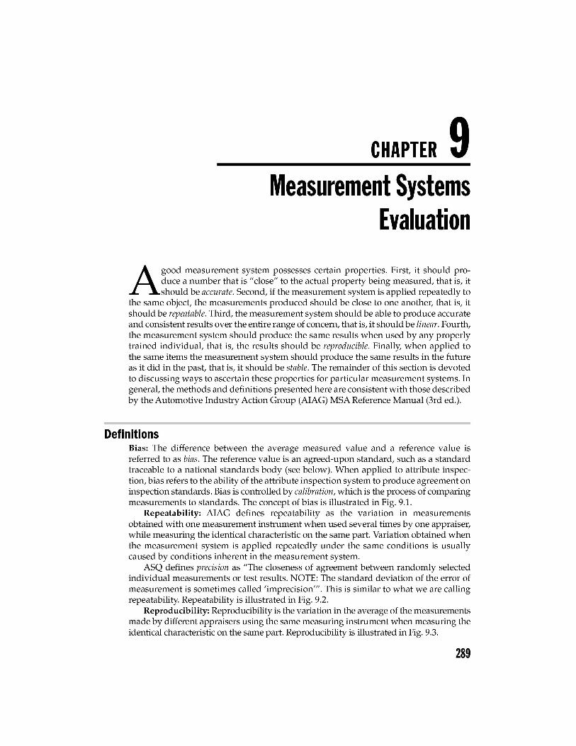
Definitions Bias: The difference between the average measured value and a reference value is referred to as bias . The reference value is an agreed-upon standard, such as a standard traceable to a national standards body (see below). When applied to attribute inspection, bias refers to the ability of the attribute inspection system to produce agreement on inspection standards. Bias is controlled by calibration, which is the process of comparing measurements to standards. The concept of bias is illustrated in Fig. 9.1.

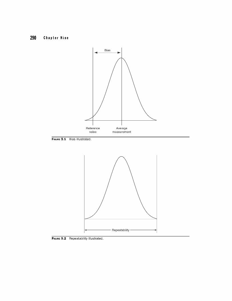
Repeatability: AIAG defines repeatability as the variation in measurements obtained with one measurement instrument when used several times by one appraiser, while measuring the identical characteristic on the same part. Variation obtained when the measurement system is applied repeatedly under the same conditions is usually caused by conditions inherent in the measurement system.

ASQ defines precision as "The closeness of agreement between randomly selected individual measurements or test results. NOTE: The standard deviation of the error of measurement is sometimes called 'imprecision"' . This is similar to what we are calling repeatability. Repeatability is illustrated in Fig. 9.2.

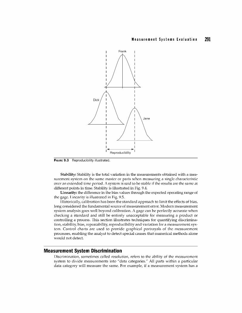
Reproducibility: Reproducibility is the variation in the average of the measurements made by different appraisers using the same measuring instrument when measuring the identical characteristic on the same part. Reproducibility is illustrated in Fig. 9.3.

289

290 C hap te r N i n e

Reference value

FIGURE 9.1 Bias illustrated.

Bias

Average measurement

1 ..... ------ Repeatability -------1

FIGURE 9.2 Repeatability illustrated.

Mea sur e men t S y stem s E y a I u a t ion 291

Frank

FIGURE 9.3 Reproducibility illustrated.

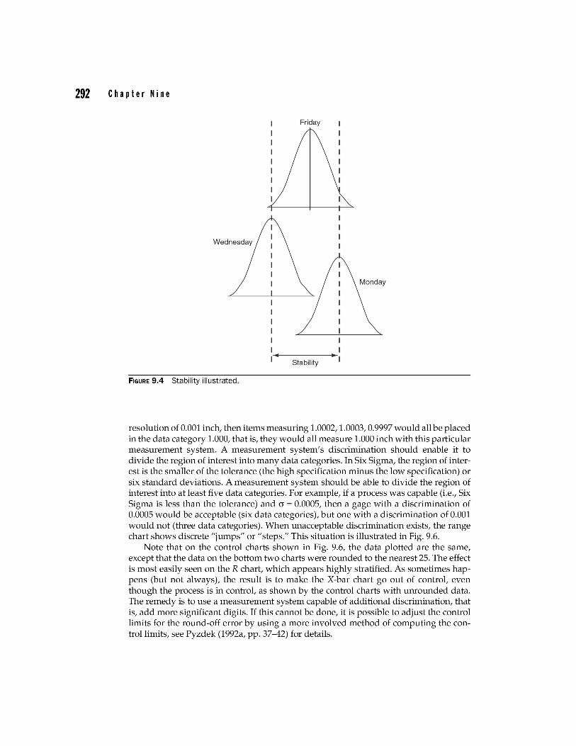
Stability: Stability is the total variation in the measurements obtained with a measurement system on the same master or parts when measuring a single characteristic over an extended time period. A system is said to be stable if the results are the same at different points in time. Stability is illustrated in Fig. 9.4.

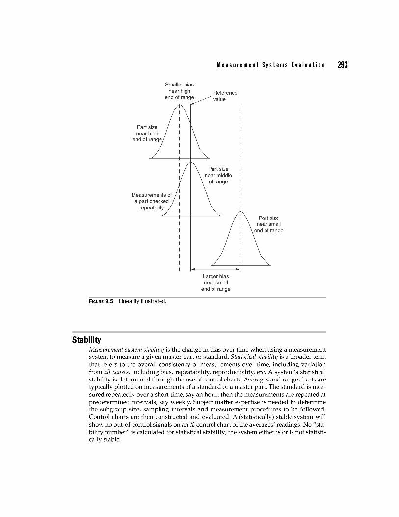
Linearity: the difference in the bias values through the expected operating range of the gage. Linearity is illustrated in Fig. 9.5.

Historically, calibration has been the standard approach to limit the effects of bias, long considered the fundamental source of measurement error. Modern measurement system analysis goes well beyond calibration. A gage can be perfectly accurate when checking a standard and still be entirely unacceptable for measuring a product or controlling a process. This section illustrates techniques for quantifying discrimination, stability, bias, repeatability, reproducibility and variation for a measurement system. Control charts are used to provide graphical portrayals of the measurement processes, enabling the analyst to detect special causes that numerical methods alone would not detect.

Measurement System Discrimination Discrimination, sometimes called resolution, refers to the ability of the measurement system to divide measurements into "data categories." All parts within a particular data category will measure the same. For example, if a measurement system has a


FIGURE 9.4 Stability illustrated.

I I I I I I

Friday

1--.. I-----------1~ Stability

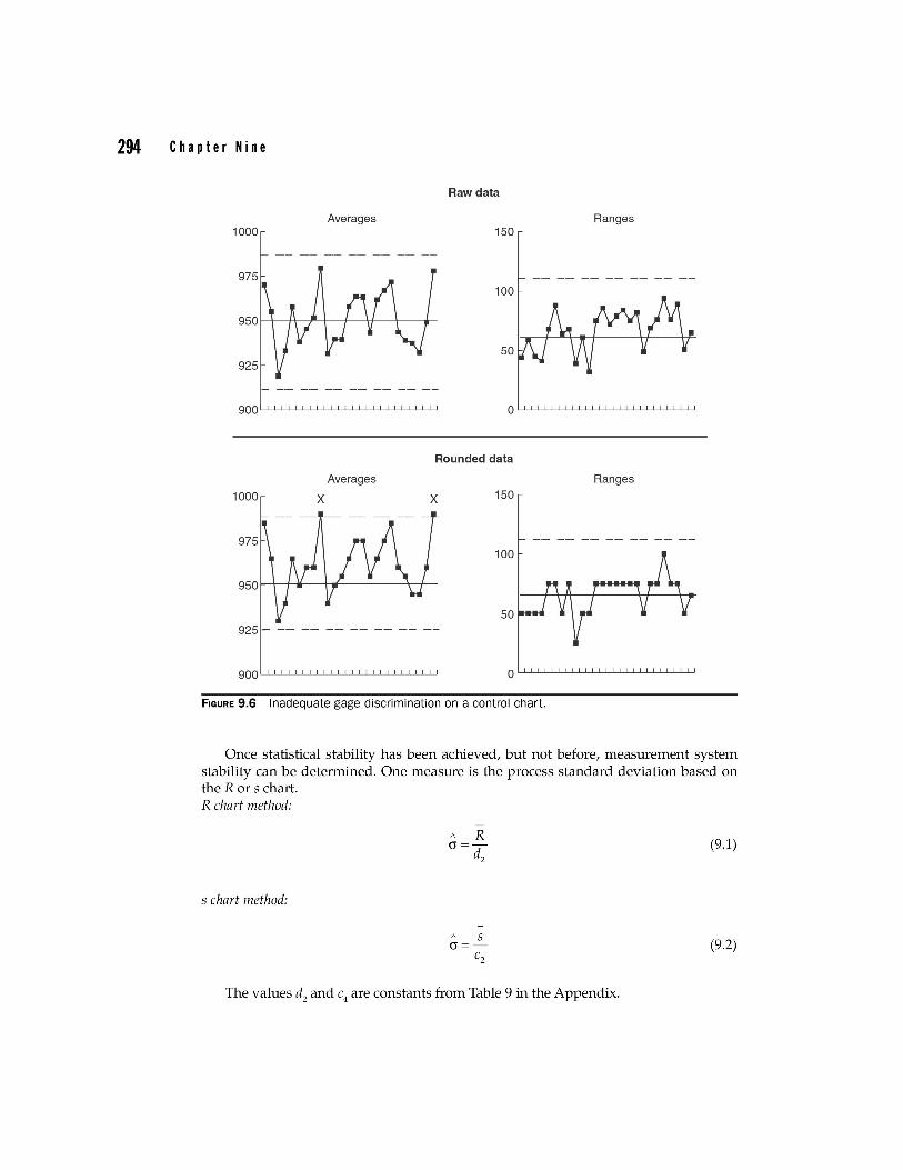
resolution of 0.001 inch, then items measuring 1.0002, 1.0003, 0.9997 would all be placed in the data category 1.000, that is, they would all measure 1.000 inch with this particular measurement system. A measurement system's discrimination should enable it to divide the region of interest into many data categories. In Six Sigma, the region of interest is the smaller of the tolerance (the high specification minus the low specification) or six standard deviations. A measurement system should be able to divide the region of interest into at least five data categories. For example, if a process was capable (Le., Six Sigma is less than the tolerance) and cr = 0.0005, then a gage with a discrimination of 0.0005 would be acceptable (six data categories), but one with a discrimination of 0.001 would not (three data categories). When unacceptable discrimination exists, the range chart shows discrete "jumps" or "steps." This situation is illustrated in Fig. 9.6.

Note that on the control charts shown in Fig. 9.6, the data plotted are the same, except that the data on the bottom two charts were rounded to the nearest 25. The effect is most easily seen on the R chart, which appears highly stratified. As sometimes happens (but not always), the result is to make the X-bar chart go out of control, even though the process is in control, as shown by the control charts with unrounded data. The remedy is to use a measurement system capable of additional discrimination, that is, add more significant digits. If this cannot be done, it is possible to adjust the control limits for the round-off error by using a more involved method of computing the controllimits, see Pyzdek (1992a, pp. 37-42) for details.

Part size near high

end of range

Measurements of a part checked

repeatedly

FIGURE 9.5 Linearity illustrated.

Stability


Reference value

Larger bias near small

end of range

Part size near small

end of range

Measurement system stability is the change in bias over time when using a measurement system to measure a given master part or standard. Statistical stability is a broader term that refers to the overall consistency of measurements over time, including variation from all causes, including bias, repeatability, reproducibility, etc. A system's statistical stability is determined through the use of control charts. Averages and range charts are typically plotted on measurements of a standard or a master part. The standard is measured repeatedly over a short time, sayan hour; then the measurements are repeated at predetermined intervals, say weekly. Subject matter expertise is needed to determine the subgroup size, sampling intervals and measurement procedures to be followed. Control charts are then constructed and evaluated. A (statistically) stable system will show no out-of-control signals on an X-control chart of the averages' readings. No "stability number" is calculated for statistical stability; the system either is or is not statistically stable.


Raw data

Averages Ranges 1000 150

100

50~ ~

Rounded data

Averages Ranges

1000 x x 150

100

50 925

FIGURE 9.6 Inadequate gage discrimination on a control chart.

Once statistical stability has been achieved, but not before, measurement system stability can be determined. One measure is the process standard deviation based on the R or s chart. R chart method:

(9.1)

s chart method:

(9.2)

The values d2

and c4

are constants from Table 9 in the Appendix.

Bias


Bias is the difference between an observed average measurement result and a reference value. Estimating bias involves identifying a standard to represent the reference value, then obtaining multiple measurements on the standard. The standard might be a master part whose value has been determined by a measurement system with much less error than the system under study, or by a standard traceable to NIST. Since parts and processes vary over a range, bias is measured at a point within the range. If the gage is nonlinear, bias will not be the same at each point in the range (see the definition of linearity defined earlier).

Bias can be determined by selecting a single appraiser and a single reference part or standard. The appraiser then obtains a number of repeated measurements on the reference part. Bias is then estimated as the difference between the average of the repeated measurement and the known value of the reference part or standard.

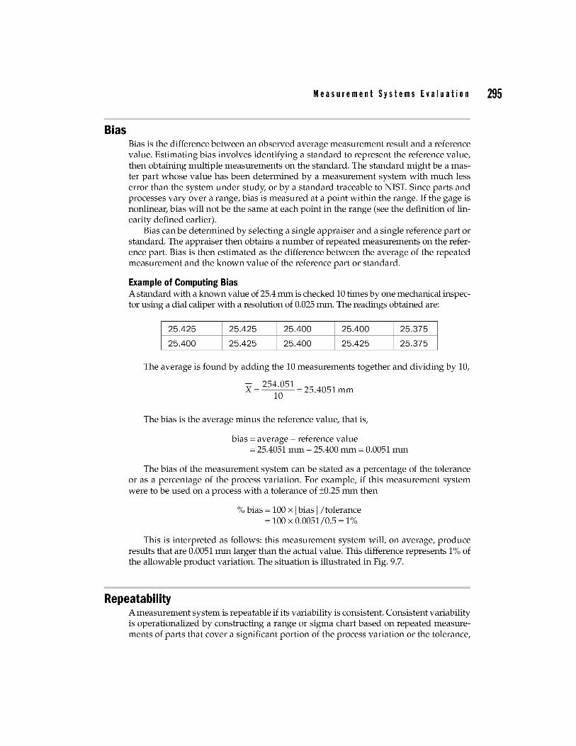
Example of Computing Bias A standard with a known value of 25.4 mm is checked 10 times by one mechanical inspector using a dial caliper with a resolution of 0.025 mm. The readings obtained are:

25.425 25.425 25.400 25.400 25.375

25.400 25.425 25.400 25.425 25.375

The average is found by adding the 10 measurements together and dividing by 10,

x = 25~~51 = 25.4051 mm

The bias is the average minus the reference value, that is,

bias = average - reference value = 25.4051 mm - 25.400 mm = 0.0051 mm

The bias of the measurement system can be stated as a percentage of the tolerance or as a percentage of the process variation. For example, if this measurement system were to be used on a process with a tolerance of ±0.25 mm then

% bias = 100 x I bias I /tolerance = 100 x 0.0051/0.5 = 1 %

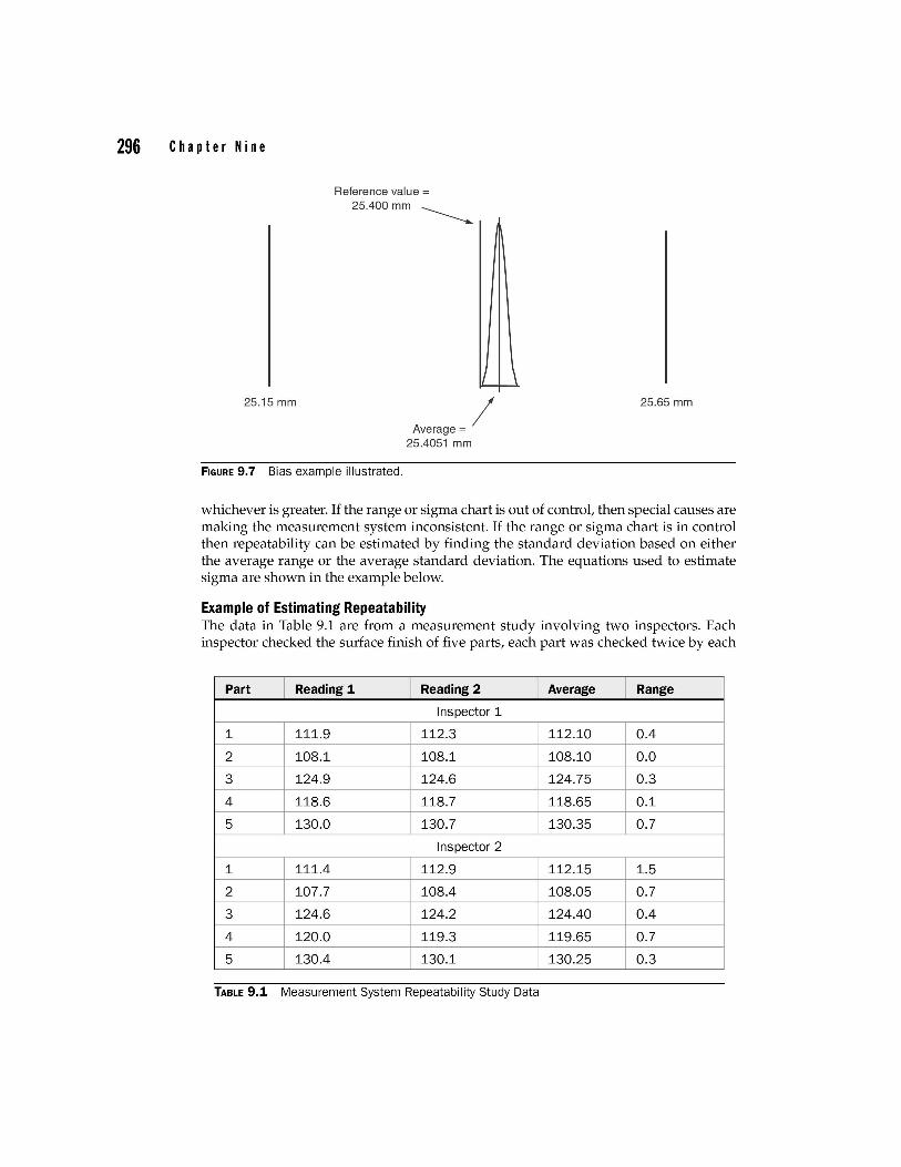
This is interpreted as follows: this measurement system will, on average, produce results that are 0.0051 mm larger than the actual value. This difference represents 1 % of the allowable product variation. The situation is illustrated in Fig. 9.7.

Repeatability A measurement system is repeatable if its variability is consistent. Consistent variability is operationalized by constructing a range or sigma chart based on repeated measurements of parts that cover a significant portion of the process variation or the tolerance,


Reference value = 25.400 mm _______

25.15 mm / Average =

25.65 mm

25.4051 mm

FIGURE 9.7 Bias example illustrated.

whichever is greater. If the range or sigma chart is out of control, then special causes are making the measurement system inconsistent. If the range or sigma chart is in control then repeatability can be estimated by finding the standard deviation based on either the average range or the average standard deviation. The equations used to estimate sigma are shown in the example below.

Example of Estimating Repeatability The data in Table 9.1 are from a measurement study involving two inspectors. Each inspector checked the surface finish of five parts, each part was checked twice by each

Part Reading 1 Reading 2 Average Range

Inspector 1

1 111.9 112.3 112.10 0.4

2 108.1 108.1 108.10 0.0

3 124.9 124.6 124.75 0.3

4 118.6 118.7 118.65 0.1

5 130.0 130.7 130.35 0.7

Inspector 2

1 111.4 112.9 112.15 1.5

2 107.7 108.4 108.05 0.7

3 124.6 124.2 124.40 0.4

4 120.0 119.3 119.65 0.7

5 130.4 130.1 130.25 0.3

TABLE 9.1 Measurement System Repeatability Study Data


inspector. The gage records the surface roughness in /.l-inches (micro-inches). The gage has a resolution of 0.1 /.l-inches.

We compute: Ranges chart

Averages chart

R = 0.51

UCL = D4R = 3.267 x 0.51 = 1.67

x = 118.85

LCL = X - A2R = 118.85-1.88 x 0.51 = 118.65

UCL = X +A2R = 118.85+ 1.88 x 0.51 = 119.05

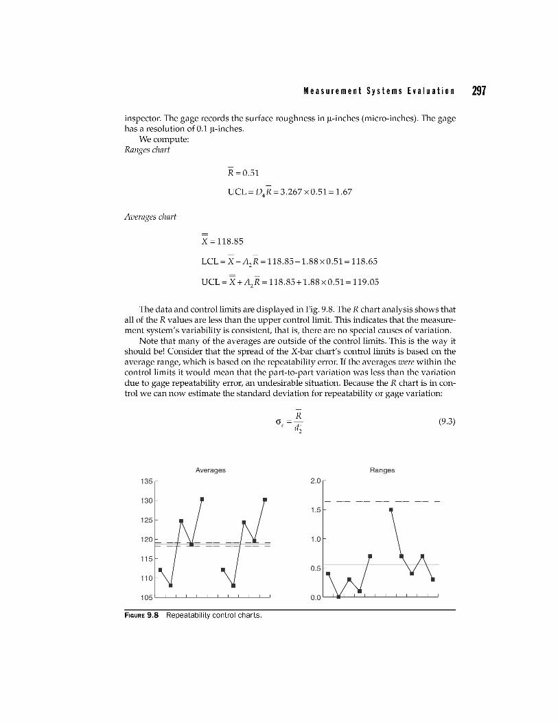
The data and control limits are displayed in Fig. 9.8. The R chart analysis shows that all of the R values are less than the upper control limit. This indicates that the measurement system's variability is consistent, that is, there are no special causes of variation.

Note that many of the averages are outside of the control limits. This is the way it should be! Consider that the spread of the X-bar chart's control limits is based on the average range, which is based on the repeatability error. If the averages were within the control limits it would mean that the part-to-part variation was less than the variation due to gage repeatability error, an undesirable situation. Because the R chart is in control we can now estimate the standard deviation for repeatability or gage variation:

(9.3)

Averages Ranges

135 2.0

130 --- --- --- --- --- -1.5

125

120 1.0

115 0.5

110

105 0.0

FIGURE 9.8 Repeatability control charts.


where d; is obtained from Appendix 11. Note that we are using d; not d2

• The d; are adjusted for the small number of subgroups typically involved in gage R&R studies. Appendix 11 is indexed by two values: m is the number of repeat readings taken (m = 2 for the example), and g is the number of parts times the number of inspectors (g = 5 x 2 = 10 for the example). This gives, for our example

R 0.51 ae = d; = 1.16 = 0.44

Report the Repeatability as percent of process sigma by dividing ae by Part to Part

Sigma (see below).

Reproducibility A measurement system is reproducible when different appraisers produce consistent results. Appraiser-to-appraiser variation represents a bias due to appraisers. The appraiser bias, or reproducibility, can be estimated by comparing each appraiser's average with that of the other appraisers. The standard deviation of reproducibility (a) is estimated by finding the range between appraisers (R) and dividing by d;. Percent Reproducibility is calculated by dividing ao by Part to Part Sigma (see below).

Reproducibility Example (AIAG Method) Using the data shown in the previous example, each inspector's average is computed and we find:

Inspector 1 average = 118.79 /.l-inches Inspector 2 average = 118.90 /.l-inches

Range = Ro = 0.11 /.l-inches

Looking in Table 11 in the Appendix for one subgroup of two appraisers we find d; = 1.41 (m = 2, g = I), since there is only one range calculation g = 1. Using these results we find d; = 0.11/1.41 = 0.078.

This estimate involves averaging the results for each inspector over all of the readings for that inspector. However, since each inspector checked each part repeatedly, this reproducibility estimate includes variation due to repeatability error. The reproducibility estimate can be adjusted using the following equation:

(~;J -(;;' = (~:!~)' __ (~_. ~_~_2 = .)0.0061- 0.019 = 0

As sometimes happens, the estimated variance from reproducibility exceeds the estimated variance of repeatability + reproducibility. When this occurs the estimated reproducibility is set equal to zero, since negative variances are theoretically impossible. Thus, we estimate that the reproducibility is zero.

Mea sur e men t S y stem s E y a I u at ion 299

The measurement system standard deviation is

report the Measurement System Error as percent of process sigma by dividing (Jm by Part to Part Sigma (see below).

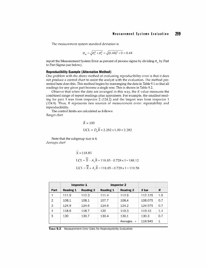
Reproducibility Example (Alternative Method) One problem with the above method of evaluating reproducibility error is that it does not produce a control chart to assist the analyst with the evaluation. The method presented here does this. This method begins by rearranging the data in Table 9.1 so that all readings for any given part become a single row. This is shown in Table 9.2.

Observe that when the data are arranged in this way, the R value measures the combined range of repeat readings plus appraisers. For example, the smallest reading for part 3 was from inspector 2 (124.2) and the largest was from inspector 1 (124.9) . Thus, R represents two sources of measurement error: repeatability and reprod ucibili ty.

The control limits are calculated as follows: Ranges chart

R = 100

UCL = D4R = 2.282 x 1.00 = 2.282

Note that the subgroup size is 4. Averages chart

x = 118.85

LCL = X - A2R = 118.85-0.729 x 1 = 188.12

UCL = X +A2R = 118.85+0.729 x 1 = 119.58

Inspector 1 Inspector 2

Part Reading 1 Reading 2 Reading 1 Reading 2

1 111.9 112.3 111.4 112.9

2 108.1 108.1 107.7 108.4

3 124.9 124.6 124.6 124.2

4 118.6 118.7 120 119.3

5 130 130.7 130.4 130.1

Averages ~

TABLE 9.2 Measurement Error Data for Reproducibility Evaluation

Xbar R

112.125 1.5

108.075 0.7

124.575 0.7

119.15 1.4

130.3 0.7

118.845 1

300 Chapter Nine

Averages Ranges

135 2.5

130 2.0 -

125 1.5

120

1.01-----'l,-----f----'<---115

110 0.5

105 0.0 '--_---'-__ L..-_---'-__ L..-_---'

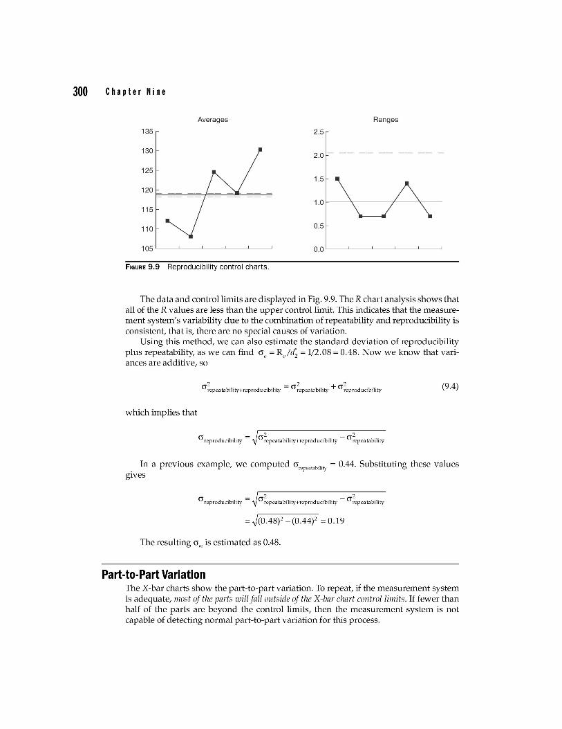
FIGURE 9.9 Reproducibility control charts.

The data and control limits are displayed in Fig. 9.9. The R chart analysis shows that all of the R values are less than the upper control limit. This indicates that the measurement system's variability due to the combination of repeatability and reproducibility is consistent, that is, there are no special causes of variation.

Using this method, we can also estimate the standard deviation of reproducibility plus repeatability, as we can find aa = Raid; = 1/2.08 = 0.48. Now we know that variances are additive, so

a;epea tability+reproducibility = a;epeatability + a;eproducibility (9.4)

which implies that

a reproducibility = 2 2 a repeatability+reproducibility - a repeatability

In a previous example, we computed a t b"l"t = 0.44. Substituting these values repeaa 11 y

gives

a reproducibility = a;epeatability+reproducibility - a;epeatability

The resulting am is estimated as 0.48.

Part-to-Part Variation The X-bar charts show the part-to-part variation. To repeat, if the measurement system is adequate, most of the parts will fall outside of the X-bar chart control limits . If fewer than half of the parts are beyond the control limits, then the measurement system is not capable of detecting normal part-to-part variation for this process.


Part-to-part variation can be estimated once the measurement process is shown to have adequate discrimination and to be stable, accurate,linear (see below), and consistent with respect to repeatability and reproducibility. If the part-to-part standard deviation is to be estimated from the measurement system study data, the following procedures are followed:

1. Plot the average for each part (across all appraisers) on an averages control chart, as shown in the reproducibility error alternate method.

2. Confirm that at least 50% of the averages fall outside the control limits. If not, find a better measurement system for this process.

3. Find the range of the part averages, R . p

4. Compute a p = R/d;, the part-to-part standard deviation. The value of d; is found in Table 11 in the Appendix using m = the number of parts and g = 1, since there is only one R calculation.

5. The total process standard deviation is found as at = Ja~ + a~.

Once the above calculations have been made, the overall measurement system can be evaluated.

1. The %EV = 100 x (a/ aT)%

2. The %AV = 100 x (ajaT)%

3. The percent repeatability and reproducibility (R&R) is 100 x (ami a/)%.

4. The number of distinct data categories that can be created with this measurement system is 1.41 x (PV IR&R).

Example of Measurement System Analysis Summary 1. Plot the average for each part (across all appraisers) on an averages control

chart, as shown in the reproducibility error alternate method. Done earlier, see Fig. 9.8.

2. Confirm that at least 50% of the averages fall outside the control limits. If not, find a better measurement system for this process. 4 of the 5 part averages, or 80%, are outside of the control limits. Thus, the measurement system error is acceptable.

3. Find the range of the part averages, R . p

R = 130.33 - 108.075 = 22.23 p

4. Compute ap

= R/ d;, the part-to-part standard deviation. The value of d; is found in Table 11 in the Appendix using m = the number of parts and g = 1, since there is only one R calculation.

m = 5, g = 1, d; = 2.48, ap = 22.23/2:48 = 8.96


5. The total process standard deviation is found as crt = Jcr~ + cr~

Once the above calculations have been made, the overall measurement system can be evaluated.

1. The %EV = 100 x (cr/crT)% = 100 x .44/8.97 = 4.91 %

2. The %AV = 100 x (cr/crT)% = 100 x 0/8.97 = 0%

3. The percent R&R is 100 x (crm/crt)%

100 ~7 % = 100 ~:!~ = 4.91 %

4. The number of distinct data categories that can be created with this measurement system is 1.41 x (PV /R&R)

46.15 1.41 x 2.27 = 28.67 = 28

Since the minimum number of categories is five, the analysis indicates that this measurement system is more than adequate for process analysis or process controL

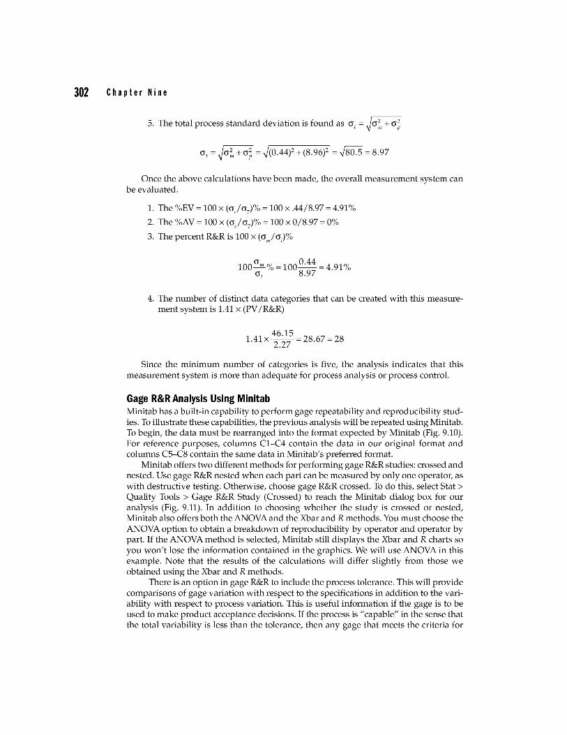
Gage R&R Analysis Using Minitab Minitab has a built-in capability to perform gage repeatability and reproducibility studies. To illustrate these capabilities, the previous analysis will be repeated using Minitab. To begin, the data must be rearranged into the format expected by Minitab (Fig. 9.10). For reference purposes, columns C1-C4 contain the data in our original format and columns C5-C8 contain the same data in Minitab's preferred format.

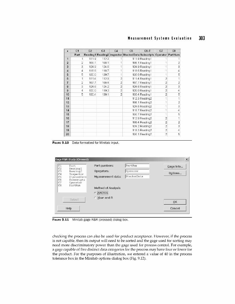
Minitab offers two different methods for performing gage R&R studies: crossed and nested. Use gage R&R nested when each part can be measured by only one operator, as with destructive testing. Otherwise, choose gage R&R crossed. To do this, select Stat> Quality Tools> Gage R&R Study (Crossed) to reach the Minitab dialog box for our analysis (Fig. 9.11). In addition to choosing whether the study is crossed or nested, Minitab also offers both the ANOVA and the Xbar and R methods. You must choose the ANOVA option to obtain a breakdown of reproducibility by operator and operator by part. If the ANOVA method is selected, Minitab still displays the Xbar and R charts so you won't lose the information contained in the graphics. We will use ANOVA in this example. Note that the results of the calculations will differ slightly from those we obtained using the Xbar and R methods.

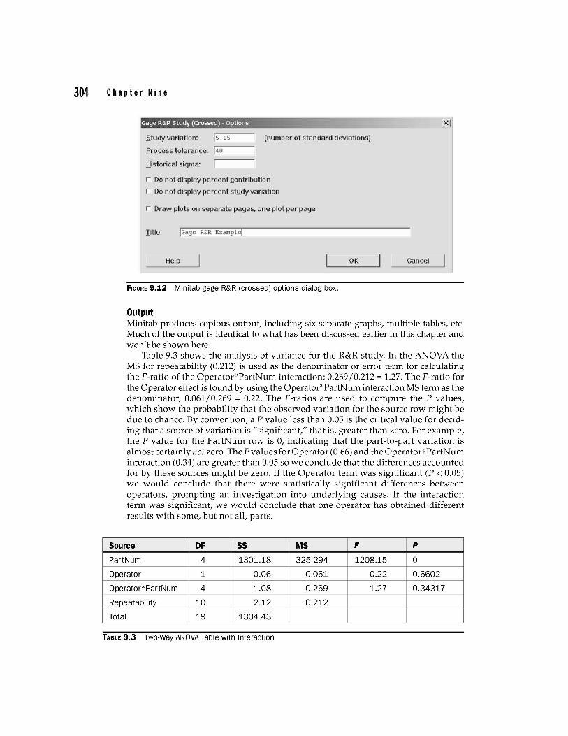
There is an option in gage R&R to include the process tolerance. This will provide comparisons of gage variation with respect to the specifications in addition to the variability with respect to process variation. This is useful information if the gage is to be used to make product acceptance decisions. If the process is "capable" in the sense that the total variability is less than the tolerance, then any gage that meets the criteria for


C1 C2 C3 C4 C5 C6-T C1 cs P:;I.rt A:u dlng1 Read ing2 Illspe(:t'Qr stack.d09ta Subscripts Op.rator P9rtNum

1 11 1.9 112.3 1 111.9 Reading l

:2

3 4

2 108.1 1081 ---t 108 1 Reading1

3 124.9 124.6 124.9 Readingl

4 11 8 .6 118.7 118.6 Reading1

5 5 130 .0 130.7 1::.0.0 Reading1

6 1 11 1.4 112.9 2 111 4 Reading1

7 2 107.7 108.4 2 107.7 R ading1

a 3 124 .6 1242 2 124.6 Reading l

51 -4 1200 1193 2 120 0 Reading1

10 13 .4 130.1 2 1::' .4 Readin 1

11 112.3 Reading2

1~ 108.1 Reading2

13 124 .6 Reading2

14 118.7 Reading2

15 130.7 Reading2

18 112.9 Reading2

17 108.4 Reading2

18 124 2 Readin 2

19 119.3 Reading2

20 130.1 Reading2

FIGURE 9.10 Data formatted for Minitab input.

Gage R&R Stud" (Crossed)

Cl C2 C3 C4 C5 C6 C7 ca

art Reading} Reading2 Inspec or StackedDate Subscript6 Operator FartNum

Select

Help

Part numbers; IPartNllm

operatolrs: II"'"O-p"-_r-a-t-or---

M~asuremerlt data: ISt ackedData

Method of .Analysis r""-'-"-'--~

r; ~~_?y

(" ~bar and n:

FIGURE 9.11 Minitab gage R&R (crossed) dialog box.

1 1

---t- 2

:3 4

5 2 1

2 2

2 3 2 4

2 5

:1 2

:3 4

1

2 1

2

2

2

5

1

2

3 4

5

Y.age Info,,,

O/!t iol1s ...

QK

Cancel

checking the process can also be used for product acceptance. However, if the process is not capable, then its output will need to be sorted and the gage used for sorting may need more discriminatory power than the gage used for process control. For example, a gage capable of five distinct data categories for the process may have four or fewer for the product. For the purposes of illustration, we entered a value of 40 in the process tolerance box in the Minitab options dialog box (Fig. 9.12).


Gage RI\,R Study (Crossed) - Options

~tudy var1iation: 115 .. 15 (number of standard deviations)

£ rocess tolerance: 1140

.!iistorical si'9ml c:l : II

r Do not display percent .Qontributi,on

r Do not display percent slydy variati on

r .Qraw piliots on s,eparate pages. one pilot per page

Ilitle: IGoge R&R Exampl eI

Help

FIGURE 9.12 Minitab gage R&R (crossed) options dialog box.

Output

QK Cancel

Minitab produces copious output, including six separate graphs, multiple tables, etc. Much of the output is identical to what has been discussed earlier in this chapter and won't be shown here.

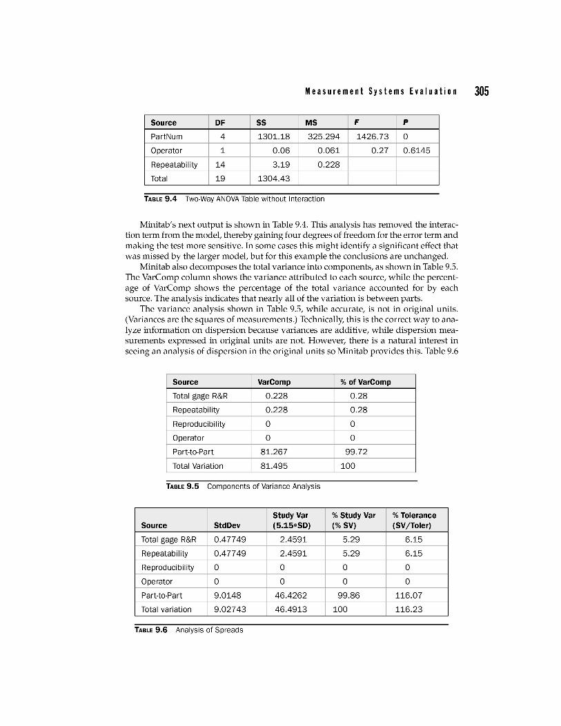
Table 9.3 shows the analysis of variance for the R&R study. In the ANOVA the MS for repeatability (0.212) is used as the denominator or error term for calculating the F-ratio of the Operator*PartNum interaction; 0.269/0.212 = 1.27. The F-ratio for the Operator effect is found by using the Operator*PartNum interaction MS term as the denominator, 0.061/0.269 = 0.22. The F-ratios are used to compute the P values, which show the probability that the observed variation for the source row might be due to chance. By convention, a P value less than 0.05 is the critical value for deciding that a source of variation is "significant," that is, greater than zero. For example, the P value for the PartNum row is 0, indicating that the part-to-part variation is almost certainly not zero. The Pvalues for Operator (0.66) and the Operator*PartNum interaction (0.34) are greater than 0.05 so we conclude that the differences accounted for by these sources might be zero. If the Operator term was significant (P < 0.05) we would conclude that there were statistically significant differences between operators, prompting an investigation into underlying causes. If the interaction term was significant, we would conclude that one operator has obtained different results with some, but not all, parts.

Source OF SS MS F I p

PartNum 4 1301.18 325.294 1208.15 0

Operator 1 0.06 0.061 0.22 0.6602

Operator*PartNum 4 1.08 0.269 1.27 0.34317

Repeatability 10 2.12 0.212

Total 19 1304.43

TABLE 9.3 Two-Way ANOVA Table with Interaction


Source OF SS MS F P

PartNum 4 1301.18 325.294 1426.73 0

Operator 1 0.06 0.061 0.27 0.6145

Repeatability 14 3.19 0.228

Total 19 1304.43

TABLE 9.4 Two-Way ANOVA Table without Interaction

Minitab's next output is shown in Table 9.4. This analysis has removed the interaction term from the model, thereby gaining four degrees of freedom for the error term and making the test more sensitive. In some cases this might identify a significant effect that was missed by the larger model, but for this example the conclusions are unchanged.

Minitab also decomposes the total variance into components, as shown in Table 9.5. The VarComp column shows the variance attributed to each source, while the percentage of VarComp shows the percentage of the total variance accounted for by each source. The analysis indicates that nearly all of the variation is between parts.

The variance analysis shown in Table 9.5, while accurate, is not in original units. (Variances are the squares of measurements.) Technically, this is the correct way to analyze information on dispersion because variances are additive, while dispersion measurements expressed in original units are not. However, there is a natural interest in seeing an analysis of dispersion in the original units so Minitab provides this. Table 9.6

Source VarComp % of VarComp

Total gage R&R 0.228 0.28

Repeatability 0.228 0.28

Reproducibility 0 0

Operator 0 0

Part-to-Part 81.267 99.72

Total Variation 81.495 100

TABLE 9.5 Components of Variance Analysis

Study Var

I

% Study Var % Tolerance Source StdOev (5.15*SO) (% SV) (SVjToler)

Total gage R&R 0.47749 2.4591 5.29 6.15

Repeatability 0.47749 2.4591 5.29 6.15

Reproducibility 0 0 0 0

Operator 0 0 0 0

Part-to-Part 9.0148 46.4262 99.86 116.07

Total variation 9.02743 46.4913 100 116.23

TABLE 9.6 Analysis of Spreads


Gage R&R example

Components of variation

120

100

80 C OJ () 60 Cii

Il..

40

20

0 ~ ~

Gage R&R Repeat Reprod

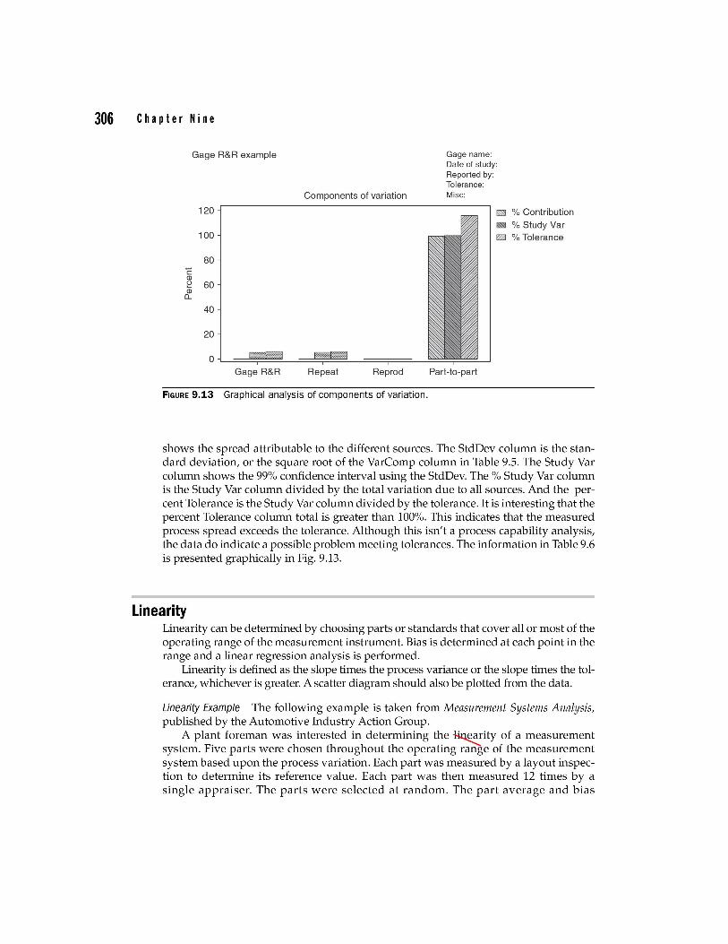
FIGURE 9.13 Graphical analysis of components of variation.

Gage name: Date of study: Reported by: Tolerance: Misc:

Part-to-part

~ % Contribution ~ % Study Var E22I % Tolerance

shows the spread attributable to the different sources. The StdDev column is the standard deviation, or the square root of the VarComp column in Table 9.5. The Study Var column shows the 99% confidence interval using the StdDev. The % Study Var column is the Study Var column divided by the total variation due to all sources. And the percent Tolerance is the Study Var column divided by the tolerance. It is interesting that the percent Tolerance column total is greater than 100%. This indicates that the measured process spread exceeds the tolerance. Although this isn't a process capability analysis, the data do indicate a possible problem meeting tolerances. The information in Table 9.6 is presented graphically in Fig. 9.13.

Linearity Linearity can be determined by choosing parts or standards that cover all or most of the operating range of the measurement instrument. Bias is determined at each point in the range and a linear regression analysis is performed.

Linearity is defined as the slope times the process variance or the slope times the tolerance, whichever is greater. A scatter diagram should also be plotted from the data.

Linearity Example The following example is taken from Measurement Systems Analysis, published by the Automotive Industry Action Group.

A plant foreman was interested in determining the linearity of a measurement system. Five parts were chosen throughout the operating range of the measurement system based upon the process variation. Each part was measured by a layout inspection to determine its reference value. Each part was then measured 12 times by a single appraiser. The parts were selected at random. The part average and bias

tom

Line

measurement systems evaluation - pyzdek...

Documents