measurements of reynolds stress profiles in unstratified … · · 2005-09-01measurements of...

+o R"-+

JOURNAL OF GEOPHYSICAL RESEARCH, VOL. 104, NO. C5, PAGES 10,933-10,949, MAY 15, 1999

Measurements of Reynolds stress profiles in unstratified tidal flow Mark T. Stacey, Stephen G. Monismith, and Jon R. Burau EnvironmGntal Fluid Mechanics Laboratory, Stanford University, Stanford, California

Abstract. In this paper we present a method for measuring profiles of turbulence quantities using a broadband acoustic doppler current profiler (ADCP). The method follows previous work on the continental shelf and extends the analysis to develop estimates of the errors associated with the estimation methods. ADCP data was collected in a n unstratified channel and the results of the analysis are compared to theory. This comparison shows that the method provides an estimate of the Reynolds stresses, which is unbiased by Doppler noise, and an estimate of the turbulent kinetic energy (TKE) which is biased by an amount proportional to the Doppler noise. The noise in each of these quantities as well as the bias in the TKE match well with the theoretical values produced by the error analysis. The quantification of profiles of Reynolds stresses simultaneous with the measurement of mean velocity profiles allows for extensive analysis of the turbulence of the flow. In this paper, we examine the relation between the turbulence and the mean flow through the calculation of u*, the friction velocity, and c d , the coefficient of drag. Finally, we calculate quantities of particular interest in turbulence modeling and analysis, the characteristic lengthscales, including a lengthscale which represents the stream-wise scale of the eddies which dominate the Reynolds stresses.

1. Introduction Turbulence in the presence of stratification and shear

plays an important role in the dynamics of shallow tidal flows like those found in estuaries. It can play an integral role in regulating barotropic and baroclinic shear flows [Peters, 1997; Stacey, 19961 and can affect b i e logical processes as well (Koseff et al., 1993). Mod- els of turbulence have been developed with varying degrees of sophistication and success [Mellor and Yamada, 1982; Lehfeldt and Bloss, 1988; Nunes- V u and Simp- son, 19941. Our ability to fully evaluate these'models has been limited by a lack of comprehensive turbulence data sets from estuarine flows.

Until the last decade, field measurements in estuaries were done using current and salinity meters moored at points around the estuary [Dyer, 1980; Bowden and Howe, 19631. These studies provided excellent time resolution, but were unable to capture spatial structures in the flows. S c h d e r and Siedler [1989] deployed a h e d tripod on the bed to measure small-scale velocity fluctu-

'Now at Department of Integrative Biology, University of

lAlso at United States Geological Survey, Sacramento, California, Berkeley.

California.

Copyright 1999 by the American Geophysical Union.

Paper number 1998JC900095. 0148-0227/99/1998JC900095$09.00

ations and profiled the water column every 30 min with a sonde to measure mean velocity and salinity. In each of these studies, turbulence measurements were limited to a couple of points near the bed or near the surface.

More recently, profiling instruments have been used to capture vertical variability in both the velocity and salinity fields. Acoustic Doppler current profilers (AD- CPs) were used by Burau et al. [1993] to study the residual flow fields in northern San Francisco Bay. An- other study using the profiling ability of the ADCPs was done by Geyer [1993], who looked at three-dimensional flows around a headland. In general, acoustic Doppler current profilers have allowed researchers to gather comprehensive data sets on the evolution of a water column. These data sets typically resolve only the mean quantities and do not address turbulent fluctuations.

A comprehensive look at vertical mixing in an estuary was given by Farmer and Smith [1980] who used acoustic backscatter to resolve the displacement of a sharp density interface in Knight Inlet. Profiles of the small-scale shear (along with an assumption of isotropy at those scales) provide estimates of the dissipation in the flow [Seim and Gregg, 19951. Measurements with a microstructure shear probe were also used by Peters, [1997] in combination with profiles of the mean velocity to estimate eddy viscosity and diffusivity [Bwch, 19771. Similar measurements have been performed by Imberger [Imberger and Head, 19941 in a variety of conditions in lakes around the world.

Gagett and Moum [1995] measured mixing efficiency

10,933

10,934 STACEY ET AL.: MEASUREMENTS OF REYNOLDS STRESS PROFILES

in tidal fronts and compared direct measurement of buoyancy flux using a towed conductivity-temperature depth profiler (CTD) and ADCP to values inferred from a microscale profiler. Gargett [1994] has also developed a method of estimating dissipation from the large scales. She used a single-beam acoustic current profiler temeasure the instantaneous fluctuating vertical velocities and defined an estimator of the dissipation based on the variance of these measurements.

A similar method to &tract turbulence statistics directly from the large scales was used by Lohmann et al. [1990] on the continental shelf. Using a pulse-to-pulse coherent acoustic Doppler current profiler, they developed ensemble profiles of Reynolds stress and eddy viscosity. In a similar experiment, van Haren et al. [1994] used a 1.2 MHz narrowband ADCP to measure eddy fluxes above a sloping bottom on the Scotian Shelf; they attributed the measured fluxes to internal wave inst+ bility. We should note here, however, a difficulty in using the narrowband ADCP for these types of measurements which arises due to biases in the noise levels between beams. Also using an ADCP, Plueddemann (19871 examined Reynolds stresses due to internal waves in the upper ocean. Finally, Lu [1997] used an ADCP in the Cordova Channel near Vancouver Island to measure Reynolds stresses and turbulent kinetic energy.

The technique used to resolve turbulence statistics in these last studies was similar to the one developed in this paper. One of the great beneiits of this method for measuring turbulent mixing (besides being noninv+ sive) is that it measures the time evolution of Reynolds stresses and mixing coefficients throughout the entire water column. In this paper, the analysis is extended to include a quantification of the error associated with the measurements. Measurements from an unstrati- bed channel flow will be used to both test the method (through comparison with theory) and to examine the turbulent characteristics of an unstratified tidal flow. The Reynolds stress profiles will be extrapolated to the bed in order to estimate values of the friction velocity. These values will then be compared to those calculated by assuming a log-layer profile for the mean velocities. Profiles of relevant turbulent lengthscales will be calculated from both the Reynolds stress profiles and the autocorrelations of the instantaneous velocity measurements. Finally, we will discuss the generalization of this approach to other flows and conditions.

2. Turbulence Measurements The data set we will discuss was collected with a 1200

kHz broadband acoustic Doppler current profiler (BB- ADCP) from RD Instruments. The BB-ADCP uses a pair of broadband encoded pulses to measure velocity throughout a water column. The pulses are transmitted from a transducer, which then functions as a receiver to collect the signal that is reflected off particles which

create a Doppler-shifted reflected signal in which the relative phase shift between the’ two reflected signals is proportional to the velocity of the reflector. Velocity measurements are done along each of four beams, which are arrayed in a Janus configuration (Figure 1). In this configuration, calculation of the two horizontal velocity components is possible as

Figure 1. Experiment configurations. (a) Janus configuration of ADCP beams. For the instrument deployed at Three Mile Slough, 6 = 20°. (b) Configura- tion of boat and ADCP deployed at Three Mile Slough. Twepoint anchoring was from the bow and the port- side stern (dotted lines). Channel walls (solid lines) not 1

move with the currents. The motions of the reflectors to scale.

STACEY ET AL.: MEASUREMENTS OF REYNOLDS STRESS PROFILES 10,935

(u3 - 214) U =

2sin9 (u1- u2)

V = 2sin9

where u1 and u2 are the beams into and out of the plane of Figure la.

The method used to calculate the turbulence statistics was outlined by fiopea [1981] for use with a one- dimensional laser Doppler anemometer and applied to ADCP data by Lohrmann et d. [1990]. The technique relies on the along-beam variances of the velocity measurements and, as such, will be referred to as the variance technique for resolving turbulent quantities.

The direct calculation of correlations between the along-beam velocities will not be used to resolve the Reynolds stresses due to inhomogeneity in the instantaneous velocity fields. As will be discussed further below, opposite beams sample the flow at locations that are separated by several meters. In the instantaneous velocity fields, there will be variations in the flow on scales defined by the turbulent eddies. Therefore, at an instant in time, it is possible (in fact, likely) that one beam will be sampling one eddy while the oppc- site beam will be sampling a merent eddy entirely, rendering direct calculation of the correlation meaning- less. The variance technique relies only on combining the statistics (mean and variance) of opposite beams. Therefore we require homogeneity between the beams only in the mean and variance of the velocity signal, an assumption that will be discussed below.

3. Definition of Method The ADCP has two pairs of opposite beams, each

inclined at 20 degrees to the vertical (other units may have 30 degree beams). As a result, as shown in Figure la, each beam measures a velocity which is actually a weighted sum of the local horizontal and vertical velocity. For beam 3 (as numbered in Figure la), the velocity measured, 213, is given bx

u3 =usine+wcosB ( 2 4 where u is the horizontal velocity in the plane formed by beams 3 and 4, w is the vertical velocity, and 9 is the angle the beams make with the vertical. Similarly, we can see that the velocity measured by beam 4 (opposite beam 3) is given by

u4 = -using + wcose (2b) Separating each velocity into a mean, where the mean

is t&en over some chosen averaging period, and a fluctuating quantity as

u = i i + u t (34

w=?i7+wt (3b)

u3 = G + U 3 I ( 4 4

u4 = T4+uqt (4b)

allows us to calculate the variance of the along-beam velocities as

~- - u4I2 = uf2sin29 + wf2cos29 - 2&7sin9cos9 (5b)

with the only difference between the two expressions being the sign on the term containing d w f .

Finally, by taking the difference of the variance of opposite beams, we can calculate the Reynolds stress exactly as

-

- - - U3t2 - u4t2 ulw' =

4 sin 9 cos 9 Similarly, the cross-stream Reynolds stress is given by

- - - u1f2 - u2t2 vfw' =

4 sin 9 cos 9

Using the variances as defined in (5a) and (5b), we can also eliminate the cross terms by summing the variances:

Using the anisotropy in the turbulent kinetic energy field (as given below, (12a) and (12b), for an unstratified channel flow), we can calculate q2 or any of its components, using the quantities in (7a) and (7b).

4. Observations and Comparison to Theory

The observations presented in this paper were collected in Three Mile Slough, a straight, narrow channel in the Sacramento-San Joaquin Delta which is tidally active but contains fresh water through most of the year. The channel is oriented directly north-south and is 3 miles long (4.8 km) and about 100 m wide [ h i , 19881. The channel actually connects the Sacramento and San Joaquin Rivers, making it unique due to the tidal forcing occurring at both ends (the tide propa- gates up both the Sacramento and San Joaquin Rivers). The prevailing winds in the summer months are east- west and therefore there is very little wave activity on the slough. For these reasons, it provided a good environment to examine unstratified tidal flow using the analysis technique shown above.

The data collection took place for 2 hours starting just after the maximum of an ebb tide (flow to the

scribed above) was deployed in the downwards-looking mode from an anchored whaler (Figure lb) and collected every ping with a frequency of about 1 Hz. The instrument was used in "mode 4" [RD Instruments, 19951, which provided a data set in which the noise

south) in August 1994. A 1200 ~ H Z BB-ADCP (de


characteristics are independent of the velocities being measured (see below, section 4.1.1 for additional discussion). Although there were no wind waves to create boat motion, there were occasional boat wakes which would be reflected in some portions of the data. The channel was approximately 9 m deep (noted from the boat's depth sounder; its data were not logged through- but the experiment) which allowed for the resolution of twenty-nine 25 cm depth cells. Although no salinity data were collected during this experiment, the channel was most likely fresh, and there should have been no

.effects of stratification, allowing the measurements to be compared to theory.

At its simplest, estuarine flow is an open-channel flow. The theory of turbulence in open channels is well developed for the case of steady, unstratified flow [Nezu and Nakagawa, 19931. For this type of flow (with a logarithmic mean velocity profile), the total shear stress (the sum of the Reynolds and viscous stresses) in the flow can be derived analytically as

where T / p is the total shear stress, Y is the molecular viscosity, and u. is a quantity known as the friction velocity and is defined by the above equation (at J = 0). The fiiction velocity is the fundamental turbulent v e locity scale for channel flow. It is usually scaled by the depth-averaged mean velocity using a constant coefficient cd as

with a typical value of c d being 0.0025 and angle brackets indicating a depth-averaged quantity.

The vertical distributions of other turbulence statistics have been analyzed by Nezu and Nakagawa [1993]. Assuming a local balance of production and dissipation, they give

ut2 = 5.29~: exp (-2-)

(9) ?d!*=cd 1/2 < z >

(104 J -

H (lob)

% - vt2 = 2.66~: exp (-2-) H

(W

(11)

- % - wt2 = 1.61~: exp (-2-) H

From which it follows that J

q2 = 9.56~: exp (-2-)

Using these expressions, we can define the anisotropy ratios of the turbulent field as

H

, . . . ... ,,.. . ' . . . .

2 5

0 cm/S Time (houn)

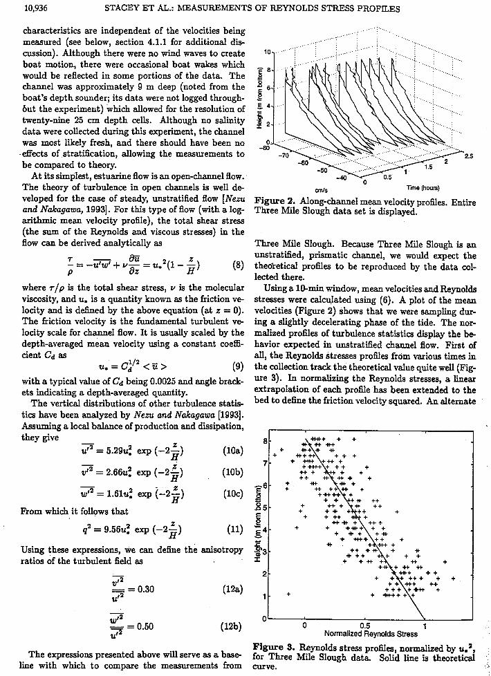
Figure 2. Along-channel mean velocity profiles. Entire Three Mile Slough data set is displayed.

Three Mile Slough. Because Three Mile Slough is an unstratified, prismatic channel, we would expect the theoretical profiles to be reproduced by the data collected there.

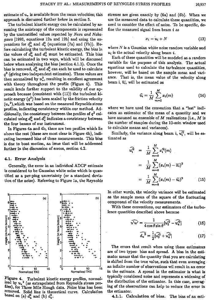
Using a 10-min window, mean velocities and Reynolds stresses were calculated using (6). A plot of the mean velocities (Figure 2) shows that we were sampling during a slightly decelerating phase of the tide. The normalized profiles of turbulence statistics display the b e havior expected in unstratified channel flow. First of all, the Reynolds stresses profiles from various times in the collection track the theoretical value quite well (Fig- ure 3). In normalizing the Reynolds stresses, a linear extrapolation of each profile has been extended to the bed to define the friction velocity squared. An alternate

I 1

I \ - (W Wt2

Ut2 i = 0.50

The expressions presented above will serve as a base- line with which to compare the measurements from curve.

0' I I 0 0.5 1

Figure 3. Reynolds stress profiles, normalized by ue2, for Three Mile Slough data. Solid line is theoretical

Normalized Reynolds Stress


estimate of u. is available from the mean velocities; this approach is discussed further below in section 5.

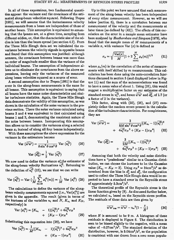
The turbulent kinetic energy can be calculated by assuming the anistropy of the components is represented by the unstratified values reported by Nezu and Naka- gawa [1993, equations 12a and 12b] and using the expressions for <: and 6", (equations (7a) and (7b)). Be- fore calculating the turbulent kinetic energy, the bias in the values of d", and d: must be estimated. This bias can be estimated in two ways, which'will be discussed below when analyzing the bias (section 4.1.1). Once the bias is removed, 4 and 6", can each be used to calculate q2 (giving two independent estimates). These values are then normalized by u:, resulting in excellent agreement with theory throughout the profile (Figure 4). This result lends further support to the validity of our approach because (consistent with (11)) the turbulent kinetic energy (q2) has been scaled by the fiiction velocity (ue2),which was based on the measured Reynolds stress profiles, indicating consistency within our method. Ad- ditionally, the consistency between the profiles of q2 calculated using d", and 6", indicates a consistency between the four beams of our instrument.

In Figures 4a and 4b, there are two profiles which lie above the rest (these are most clear in Figure 4b), indicating increased bias of these measurements. This bias is due to boat motion, an issue that will be addressed further in the discussion of errors, section 4.2.

4.1. Error Analysis

Generally, the error in an individual ADCP estimate is considered to be Gaussian white noise which is quan- tified as a per-ping uncertainty (or a standard d e v b tion of the noise). Referring to Figure la, the Reynolds

O! I 0 5 10 15

Normalized TKE

5541 A :+ +

1/ +%+ +H+ + +:+++ CC * 1

"0 5 10 15 Normalized TKE

Figure 4. Tu.&ulent kinetic energy profiles, normalized by u , ~ (as extrapolated from Reynolds stress pr* file), for Three Mile Slough data. Noise bias has been removed. Solid line is theoretical curve. Calculation

on (a) d", and (b) 4.

stresses are given exactly by (6a) and (6b). When we use the measured data to calculate these quantities, we need to consider the effect of noise. To be specific, define the measured signal from beam i as

~j = Li + N (13)

where N is a Gaussian white noise random variable and ui is the actual velocity along beam i.

Each of these quantities will be modeled as a random variable for the purpose of this analysis. The actual equations used to calculate the turbulence quantities, however, will be based on the sample mean and variance. That is, the mean value of the velocity along beam i, K , will be estimated as

where we have used the convention that a "hat" indicates an estimator of the mean of a quantity and we have assumed an ensemble of M realizations (i.e., M is the number of samples during the 10-min window used to calculate means and variances).

Similarly, the variance along beam i, q, will be estimated as

1 = z c (.i(rn) - q2

m=O

, M

m=O

In other words, the velocity variance will be estimated as the sample mean of the square of the fluctuating component of the velocity measurements.

With these conventions, our estimators of the turbulence quantities described above become

The errors that result when using these estimators are of two types: bias and spread. A bias in the estimator means that the quantity that you are calculating is shifted from the true value, such that even averaging an infinite number of observations wil result in an error in the estimate. A spread in the estimator is what is typically considered noise and represents a widening of the distribution of the estimator. In this case, averaging of the observations can help to reduce the error in the estimator. 4.1.1. Calculation of bias. The bias of an esti-


mator is the dxerence between the expected value of the estimator and the quantity it is attempting to measure. To be specific, the bias in an estimator of the variable y is given by E(@) - E(y), where we have d e fined E(z) to be the expected value of the variable z [Bendat and Piersol, 19861.

Taking the expected value of (16) and (17) gives ,

E(u‘w’) = 1 [E(u2) - E(u?)] (18) 4cos8sin8.

E ( Z ) = $ E ( G ) + E ( Z ) ]

Examining (15), we see that the expected value of u? is equivalent to the variance in the measurements of velocity. That is,

n

E(UT) = var (Zj)

= var ( U i ) + var ( N )

+ 2 cov (Ui ,N) (20)

where we have applied (13). When operating in mode 4, the BB-ADCP produces velocity measurements for which the error is dominated by Doppler “self-noise,” not flow-dependent components. The flow-dependent errors are very small relative to the self-noise, and the noise can be assumed to be independent of the velocities being measured. This should be contrasted with modes 5 and 8, where flow-dependent errors are comparable to the self-noise and indepedence between flow parameters (such as turbulent fluctuations) and noise can not be assumed. Because our data were collected in mode 4, we can safely assume that Cov (u i ,N) = 0. Thus we have that

E(u?) = ui2 + ON or, the estimate of velocity variance is biased from its true value by an amount equal to the noise variance

Substituting (21) into (18) and (191, we get the following expressions for the expected values of our estimators:

(21) 2 n -

U N 2 .

- - - [@ - u 3 = u‘w’ (22)

1 4cos8sin8

E(u&?) =

= 2L’2sh2 8 + z c o s 2 8 + ON2 (23)

Thus the estimator of the Reynoldsstress is unbiased by Doppler noise, but estimators which are related to the kinetic energy (4, 4) are biased by an amount equal to the variance of the noise (ON’). Returning to Figure 3, we note that although the method of normalizing the Reynolds stresses constrains the profiles to approach 1 at the bed, the surface values are not

proach zero (within the expected noise level, see below) is consistent with the Reynolds stress estimator being unbiased by Doppler noise. To estimate the bias in the kinetic energy variables (e, G), we examine his- tograms of values of d% and d”, (Figure 5). There are no values of 4 or d: which are less than 28.8cm2/s2 and only two values less than 34cm2/s2. We therefore select a value of 34cm2/s2 to be representative of the noise variance, U N ~ . This is equivalent to a per-ping error of 5.8?, which is consistent with the value reported by RD Instruments [1995].

As an additional check on this bias estimate, we note that this bias has been removed in calculating the turbulent kinetic energy as displayed in Figures 4a and 4b. Comparing these profiles with theory show no persis- tent bias (other than that due to boat motion, which is discussed below), suggesting that we have correctly removed the bias due to instrument noise. Additionally, the consistency between the distributions of d”, and d”, provides evidence that all four beams of the instrument have similar noise characteristics, as we would expect. 4.1.2. Calculation of spread. In analyzing the

bias of the estimators we took the expected values of (16) and (17). Analogously, the spread in the estimators will be defined by the variance of those same equations. The errors in using (16) and (17) to estimate the turbulence quantities will be defined by the standard deviation (or variance) of those equations. From (16) and (17) we have:

[var (2) 1 16 sin2 6 cos2 6

var (u‘w’) =

1 n

-[Var (u?) +var (u?)

0.2 I 1

“0 10 20 30 40 50 60 d: (cm2/s2)

dt (cm2/s2)

Figure 5. Histogram of frequency of values of d: and n 3 constrained. The fact that the near surface values a p a,. 3


In all of these expressions, two fundamental quantities appear: the variance and the covariance of the estimated along-beam velocities squared. Following nopea [1981], we will assume that the instantaneous velocity measurements horn a beam are independent of those of another beam. This assumption is equivalent to assuming that the beams are, a t a given time, sampling from different eddies, or, that the characteristic size of the eddies is less than the beam spread (see section 4.2). From the Three Mile Slough data set we calculated the covariance between the velocity signals in opposite beams and found that this assumption was justified: although nonzero, the covariance between beams was more than an order of magnitude smaller than the variance of the individual beams. The assumption of independence allows us to eliminate the covariances from the above expressions, leaving only the variances of the measured along beam velocities squared as a source of error.

A second assumption due to nopea [1981] is that the error in the along-beam measurements is the same for all beams. This assumption is equivalent to saying that d beams have the same noise characteristics and similar turbulence statistics. Again, the Three Mile Slough data demonstrate the validity of this assumption, as was shown in the calculation of the noise variance in the previous section. There the noise variance calculated using beams 3 and 4 was equivalent to that calculated using beams 1 and 2, demonstrating the consistent nature of the noise between beams. Incorporating this assump tion allows us to consider the variances along a selected beam xi instead of along all four beams independently.

With these assumptions the above expressions for the variance in the estimators become

n

Var (ur) (26) 1

8 sin2 8 cos2 8 var (u’w‘) =

n

(27) - 1

2 We now need to define the variance ofihe estimator of the along-beam velocity fluctuations uT. Returning to the definition of u? (15); we see that we can write

var (4) = - var (Ui2)

h

1 M

M 1 M

Var (3) = Var (- C xf((m)) = - Var (z:’) (28) m=O

The calculations to define the variance of the along- beam velocity measurements squared (i.e., Var(zi2)) are given in the appendix. The result (given in terms of the kurtoses of the variables ui and N, K,, and KN, respectively) is

Substituting this expression into (28), we have

Up to this point we have assumed that each measurement of the along-beam velocity has been independent of every other measurement. However, as we will see below (section 5), there is a correlation between one measurement of the ve1oci;ty and the measurements at later times (as defined by (43)). The effects of this correlation on the error in a sample mean estimator have been analyzed by Heathershaw and Simpson [1978], who found that the sample mean of M measurements of a variable x , with variance Var ( x ) is defined as

M Var ( x )

m=l

where p,(m) is the correlation of the series of measurements with itself shifted by m measurements. This calculation has been done using the auto-correlation func: tions discussed in section 5 (and displayed below in Fig- ure 11) and the sum of the autocorrelations was found to have a mean value of about 1. Using (31), this would suggest a multiplicative factor on our estimates of the standard errors in ui2, and hence u%’ and 4, of 1.7 (or a factor of 3 in the variance).

This factor, along with (30), (26), and (27) completely define the random errors present in the calculation of the turbulence characteristics. For completeness, they are

h n

[(KUi - 1)(T)’ 3

8M sin2 8 cos2 8 h

var (u’w’) =

3 -[(Ku, - 1)($)’ 2M

n

var (6”) =

+ 4 T a N 2 + (KN - l)QN4] (33)

Assuming that both the velocity and noise distributions have a “peakedness” similar to a Gaussian distribution, we can choose the kurtoses to be the Gaussian value (K,,, = KN = 3). Using UN’ = 34cm2/s2 as d e termined from the bias in d”, and d i , the configuration used to collect the Three Mile Slough data would be expected to have a standard error in the Reynolds stress of approximately 5.3cm2/s2.

The theoretical profile of the Reynolds stress is the linear function given by (8). As discussed further below, we calculated u* based on the Reynolds stress profiles. The residuals of these data are then given by

- (34)

2 u’w’tes = ” - u*2(1- -) H where H is assumed to be 9 m. A histogram of these residuals is displayed in Figure 6. The distribution is seen to be biased slightly to the negative, with a mean value of -0.27cm2/s2. The standard deviation of the distribution, however, is 5.04cm2/s2, so the population is consistent with one drawn from a zero mean popul&

10,940 STACEY ET AL.: MEASUREMENTS OF REYNOLDS STRESS PROFILES I

try in the sequence is less than an earlier entry [Bendat and Piersol, 19861. Again, this quantity is used to accept or reject the hypothesis of stationarity at the 95% coddence level. Applying this analysis to this data set [see Stacey 19961 shows that the flow being examined is statistically stationary at the 20-30 min timescale to the 95% confidence level in all four beams. Therefore over a 10-min window the assumption of temporal stationarity is justified.

A second assumption is the spatial homogeneity of the flow. Spatial homogeneity requires that, at a given depth, opposite beams are sampling turbulence fields that have the same statistics (because we use opposite beams to resolve a single turbulence statistic). The maximum spread of the beams Zf, is given by

Reynolds stress error

Figure 6. Histogram of errors in Reynolds stress estimates (difference between measured value and theoretical value), for Three Mile Slough data set. Solid line (with asterisks) is equivalent Gaussian (see text for discussion).

tion. The equivalent Gaussian distribution (with mean of -0.27cm2/s2 and standard deviation of 5.04cm2/s2) is also displayed and a slight negative skewness of the errors might be evident, but more samples would be nec- essary to fully analyze these higher moments. The standard deviation of the error distribution is also consistent with the value predicted by error analysis of 5.3cm2/s2, which suggests that our understanding of the noise characteristics of the Reynolds stress estimates is correct.

4.2. Other Sources of Error

Inherent in the calculations of the turbulent statistics is the assumption of temporal stationarity over the 10- min window used to define the velocity variances. Vi- olation of this assumption would provide an additional source of error. The condition of stationarity requires that both the mean and the variance of the along-beam velocities be stationary for the period of time used in calculating the turbulent quantities (i.e., the flow is not evolving on a timescale shorter than that used to calculate the turbulence information).

In order to test the temporal assumption, the mean and variance of the along-beam velocities were calculated every 30 s. Then, following Sovlsby [1980], both a run test and a reversals test were applied to the series of 30 s moments. The run test for stationarity counts the number of sequences (or runs) within a series which re- main on one side of the median value (or, alternatively, it counts the number of times the series crosses the median value) [Shanmugan and BreipohZ, 19881. The number of runs (along with the sequence length) determines the statistical certainty with which you can accept or reject the hypothesis of stationarity. For our analysis, a 95% coddence threshold was used. The reverse ar- rangements test counts the number of times that an en-

X C ~ = 2HsinB (35) where H is the depth of the water column (or range of data collection if less than the depth). For the Three Mile Slough data set, this results in a maximum beam spread of 6.2 m. The lengthscale for variations in the mean velocity fields, and hence turbulence statistics, is set by bathymetric variations. At this site, this lengthscale is of the order of hundreds of meters, providing suEcient homogeneity for our calculations.

An additional bias may be due to the vertical resolution of the ADCP. The ADCP performs some spatial averaging within its bins, thus limiting the range of eddies for which it wilI retain information. In the case of 25 cm bins, eddies of size smaller than (approximately) 50 cm will not be well resolved by the ADCP and the variance in the velocity field will be reduced. As a result, the turbulence quantities, both the -turbulent kinetic energy (TKE) and the Reynolds stress, wil l be biased downwards by an amount equal to the sub- depth-cell contributions to these quantities. Because both of these quantities (the TKE and the Reynolds stress) are dominated by the large eddies, this error is believed to be small. However, this bias may be a factor in the downwards bias of the friction velocity based on the Reynolds stresses in the first portion of the current data set; as a result, this bias is an area of on-going research.

Finally, the profiles which lie above the expected curve in Figure 4 represent additional noise introduced into the system by the motion of the boat on which the ADCP was mounted. This additional variance was not represented in the Reynolds stress profiles because the estimator of the Reynolds stress is unbiased (however, it coincided with the profiles for which low values of the friction velocity were estimated). The variance which is induced by the rocking of the boat is quantifiable given information about the motion of the boat. For the Three Mile Slough data set, we have time series of pitch, roll, and heading from the ADCP itself.

The effects of nonzero pitch and roll on this type of analysis were analyzed by uan Haren et al. [1994]. They considered the biases that are induced if pitch and roll


were off from the expected angles slightly. However, when calculating the variance of the velocity variances, it is also important to examine the variance induced by the motions of the sensor. These variances will be produced by two types of motion: rotation and translation.

The variance induced by rotation of the vessel will be dependent on the time derivative of the pitch angle (A) and roll angle (4,) and on the moment arms of the instrument from the centers of pitch and roll (Ip and I,, respectively). With these v&iables, the induced variance will be proportional to the quantity

For the Three Mile Slough deployment, the time s e ries of (dp)2 and (d,)2 are displayed in Figure 7. The primary motion is clearly in the roll component of the motion, which had a small (but unmeasured) moment arm. In fact, the TKE profile from hour 2 was not one of the ones exhibiting bias, as would be expected based on the pitch and roll measurements. The two most biased profiles in Figures 4a and 4b are at times 0.3333 hour and 0.66667 hour into the deployment, a period in which there is very small variability in the pitch and roll.

These data indicate that translational motion due to vertical movements of the boat could be more important in setting the level of bias in the velocity measure ments. Such motion will bias all four beams equally, which is consistent with what is seen in the data at hours 0.3333 and 0.6667. It is also possible that such motion (contaminating all beams equally) would overwhelm the variance due to turbulent motions and lead to a downwards bias in the Reynolds stresses (because the stresses are based on the differences in the variances), which is consistent with the low values of the friction velocity discussed below. Vertical translation of the boat is a difticult quantity to measure, as it does

- -

Figure 7. Time series of variance in time derivatives of Pitch (dashed line) and roll (solid line).

not necessarily correlate with either pitch or roll. As will be discussed further below (section 6), the quantification of these motions could be critical in future studies using shipmounted ADCPs.

5. Analysis of Turbulence As discussed above, the fundamental velocity scale in

open channel flow is the friction velocity u,. With the data from Three Mile Slough, we were able to estimate this quantity in two independent ways: the fist using the mean velocities, the second using the Reynolds stresses. The expression for mean velocity in an unstratified open channel follows the well-known logarithmic law: . .

(37)

where u. ( t ) is the time series of the friction velocity, zoa is an o&et in the vertical position and z, is the roughness lengthscale. We have assumed that the roughness lengthscale is independent of time, which is valid for the timescales under consideration.

The parameters u,(t), zoa and z, were adjusted to provide the best fit to the data in the least squares sense; most of the resulting proiiles are displayed in Figure 8. A similar approach was applied by h e c k and Lu [1997] to a tidal channel in near Vancouver Island. They fit the logarithmic profile to the bottom portion of the water column, where the water column was u11- stratified. Because the Three Mile Slough water column was unstratified, we used the entire profile to fit the log profile.

The values of u, will be discussed below; the roughness lengthscale (2,) converged to a value of 8.2 cm and the vertical offset placed the first measurement 1.1 m above the bed, consistent with our expectations. The high value of .tr may indicate the presence of some small sand waves.

In order to quantify the errors on u,, zoa and .z;, we applied parametric bootstrapping to the data set [Efron and Tibshimni, 1993, pp. 53-56]. The mean velocity data were resampled with the addition of noise, which was assumed to be Gaussian, and the curve fit was re- peated, resulting in distributions of each of the fitted parameters. The standard deviation of the Gaussian noise was determined from (31), using ug = 34 cma/sa, M = 480 samples and, as discussed above, a factor of 1.7 to account for the autocorrelation of the velocity measurements. The result of this calculation was a standard error in the mean velocities of uu = 0.46 cm/s. The resulting distributions of U. are shown on the graph of friction velocity (discussed below; Figure 9). The standard errors of the o&et (z,a) and the roughness length (+) were 3 and 0.4 cm, respectively.

The Reynolds stresses were used to estimate u, by extrapolating linearly to the bottom (using the best linear fit in the least squares sense). This is a fun- damentally different approach to using logarithmic fits

10,942

4.5

4 -

3.5

STACEY ET A.L.: MEASUREMENTS OF REYNOLDS STRESS PROFILES

A -

V

- V

0- 50 60 70

8

6

4

2

0 50 60 70

0- 50 60 70

0- 0- 50 60 70 50 60 70

0- 0- 50 60 70 50 60 70

Figure 8. Samples of log fits to nine profiles. All horizontal axes are cm/s; all vertical axes are height above bottom in meters.

to mean velocity profiles to get u.. Here we rely ody on the shear stress itself. In addition to the value of u., the curve fit also adjusts the location of the surface, or “zero point” of the Reynolds stress profiles. Once again, to quantify the errors on each of these estimates, parametric bootstrapping was applied to the data. For the Reynolds stresses, a standard error of 5.3 cm2/s2 was chosen, consistent with the above error analysis.

The values of the friction velocity are discussed below; the estimates of the surface position had a mean value of 8.33 m with a standard error of 0.67 m. This result is consistent with the estimate of water column depth from the depth sounder of 9 m (there is no error estimate for the depth sounder measurement). Only 3 of the 13 profiles resulted in curve-& which were nonphysical due to negative values of either the friction velocity squared or the position of the surface. These profiles (numbers 1, 6, and 8) have been discarded for the continued discdon.

Each estimate of the time development of the friction velocity is shown in Figure 9. The time development of the estimates based on the mean velocities shows the effects of the slight deceleration, as the friction velocities also decrease slightly. The d u e s based on the Reynolds stress profiles show more scatter than the ones based on mean velocities, but the magnitude is similar. The increase in friction velocity (based on the Reynolds stress profiles) over the 2 hour period may be an effect of the deceleration of the flow, which has been seen to be associated with an increase in Reynolds stress activity [Gross and Nowell 19851.

During the first hour of the study, several of the values of u. predicted by the Reynolds stress profiles fall below those from the mean velocities. Even account- ing for the variation in these estimates (denoted by the triangles in Figure 9), the two estimates of the friction velocity appear to be somewhat inconsistent. Over the first hour of the deployment, in particular at times 0.333 and 0.667, the friction velocity based on the Reynolds stresses appears to be biased low relative to the values

7.4- 1

I 0.5 1 1.5 2 2.5 -

Time (hours) 3t!l

Figure 9. Time series of U. based on Reynolds stress

(triangles) based on bootstrapping; and logarithmic fits to mean velocity measurements (solid line), plus and minus 2a limits (dashed line) based on bootstrapping.

:

5 3

profiles: mean values (asterisks) and plus and minus 2a .. .t;

E


based on the mean profile, which may indicate an un- known source of bias, perhaps due to boat motion (see additional discussion below). For the last hour and a half of the deployment, however, the agreement between the two values is encouraging.

Another way of looking at the friction velocity uses the drag coefficient c d which is defined as the square of the ratio of the friction velocity to the depth-averaged mean velocitv:

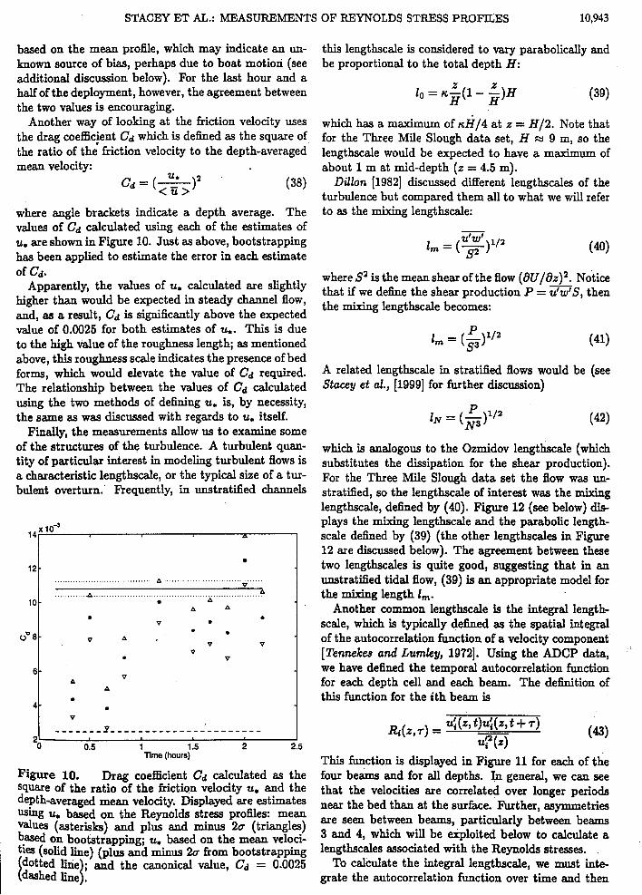
where angle brackets indicate a depth average. The values of c d calculated using each of the estimates of U. are shown in Figure 10. Just as above, bootstrapping has been applied to estimate the error in each estimate

Apparently, the values of u. calculated are slightly higher than would be expected in steady channel flow, and, as a result, c d is significantly above the expected value of 0.0025 for both estimates of u.. This is due to the high value of the roughness length; as mentioned above, this roughness scale indicates the presence of bed forms, which would elevate the d u e of c d required. The relationship between the values of c d calculated using the two methods of defining u, is, by necessity, the same as was discussed with regards to U. itself.

Finally, the measurements allow us to examine some of the structures of the turbulence. A turbulent quantity of particular interest in modeling turbulent flows is a characteristic lengthscale, or the typical size of a turbulent overturn.' Fkequently, in unstratified channels

Of c d .

I4F----=7 -I ...................................... A ....................................

V

A A A

............ ............................................................. A ,A..

10 I

2' I 0 0.5 1 I .5 2 2.5

Time (hours)

Figure 10. Drag coefficient c d calculated as the Square of the ratio of the fiictiqn velocity u. and the

are estimates

minus 20. (triangles) u. based on the mean veloci- minus 2u from bootstrapping

value, cd = 0.0025

this lengthscale is considered to vary parabolically and be proportional to the total depth H:

2 I I0 = ~ - ( l - -)H

H H (39)

which has a maximum of K H / ~ at z = H/2. Note that for the Three Mile Slough data set, H M 9 m, so the lengthscale would be expected to have a maximum of about 1 m at mid-depth ( z = 4.5 m).

Dillon [1982] discussed different lengthscales of the turbulence but compared them all to what we wil l refer to as the mixing lengthscale:

where S2 is the mean shear of the flow (8U/&)2. Notice that if we define the shear production P = zl"S, then the mixing lengthscale becomes:

A related lengthscale in stratified flows would be (see Stecey et al., [1999] for further discussion)

p 1/2 IN = (-) N3

which is analogous to the Ozmidov lengthscale (which substitutes the dissipation for the shear production). For the Three Mile Slough data set the flow was unstratsed, so the lengthscale of interest was the mixing lengthscale, defined by (40). Figure 12 (see below) dis- plays the m k h g lengthscale and the parabolic lengthscale defined by (39) (the other lengthscales in Figure 12 are discussed below). The agreement between these two lengthscales is quite good, suggesting that in an unstratified tidal flow, (39) is an appropriate model for the mixing length I, .

Another common lengthscale is the integral lengthscale, which is typically defined as the spatial integral of the autocorrelation function of a velocity component [Tennekes and Lumley, 19721. Using the ADCP data, we have defined the temporal autocorrelation function for each depth cell and each beam. The definition of this function for the ith beam is

This function is displayed in Figure 11 for each of the four beams and for all depths. In general, we can see that the velocities are correlated over longer periods near the bed than at the surface. Further, asymmetries are seen between beams, particularly between beams 3 and 4, which will be exploited below to calculate a lengthscales associated with the Reynolds stresses.

To calculate the integral lengthscale, we must inte- grate the autocorrelation function over time and then


1

i a 4 0.5 5 0

. L

0 10 lo 0

Height (m) ’ Time (s)

zu 0 Height (m) Time (s)

Figure 11. the autocorrelation at a given depth and lag time. Calculations based on measurements from (a) beam 1, (b) beam 2, (c) beam 3 and (d) beam 4.

Autocorrelation function for each of the four beams. Each plot shows contours of .

apply Taylor’s hypothesis of frozen turbulence [Kundu, 19901 to define the integral lengthscale in the x direction

W as

&(%) = u(X) 1 &(%T)dT (44) 0

where i indicates the beam being used, and the s u b script x is used to specify that it is the lengthscale in the x direction.

In Figure 12, a l l of the above described lengthscales are displayed. All four integral lengthscales increase away from the bed as expected, and, as mentioned above, the mixing lengthscale ( I , ) matches the parabolic lengthscale ( lo ) remarkably well. In general, we can say that all four integral lengthscales are larger in magnitude than either the mixing lengthscale or the parabolic lengthscale. This is not unexpected, however, based on direct numerical simulation of sheared turbulence. The database of Holt et al., [1992] has been used to quantify both an average integral lengthscale and the mixing lengthscale calculated using (40). These data were cre- ated in unstratsed conditions and also demonstrates an integral lengthscale which is larger than the mixing lengthscale. In the Holt data, the ratio of the average integral lengthscale to the mixing lengthscale is about 2, very similar to the ratio seen in the Three Mile Slough data set.

Examining the definition of the autocorrelation of the along-beam velocities (equation (43)), we can write for beam 3,

Expanding U: using (2a) gives

U i ( t ) U h ( t + 7) = U2U’(t)U’(t + T )

+ b 2 d ( t ) d ( t + 7) + ah’(t)w‘(t + 7 ) . _ . + ahu’(t)u’(t + 7) (46)

I 50 1’00 150 200 250

crn o:

Figure 12. Profiles of lengthscales - based on entire data set, mixing lengthscale, 2 , = ( -u’w’ /S~) ’ /~ (solid h e ) , Integral lengthscales based on integration of aut* correlation function of beam 1 (line with pluses), beam 2 line with circles), beam 3 (line with asterisks), beam 4 line with triangles), and the traditional parabolic pro-

file, 20 = d a / H ( l - z / H ) (dashed line).


where a = sin9 and b = cos9, and we have dropped the I from the argument of each velocity component for brevity.

The symmetry of the correlation function requires that

which allows us to rewrite (46) as

U‘(t)W’(t + T ) = U’(t + T)W’(t) (47)

ui(t)ui(t + T ) = a2u’(t)u‘(t + T )

+ Pwl(t)w’(t + T )

+ 2abu’(t)w‘(t + T ) (48)

Performing the same analysis on the velocity fluctuations along beam 4 results in

ui(t)ui(t + T ) = a2u‘(t)u’(t + T )

+ b2w’(t)w’(t + T) - 2 a ~ ( t ) w ’ ( t + T ) (49)

where, just as when calculating the Reynolds stresses, the difference between these two expressions is in the sign on the cross-correlation term.

Because these autocorrelations are statisical quantities, we can again involce the spatial homogeneity ol the turbulence statistics and combine these two quantities to isolate the cross correlation: ’

u;(t)ui(t + T ) - ui(t)ui(t + T ) =

4abu’(t)w’(t + 7) (50)

Returning now to the definition of the integral lengthscales &,= and Ad,, (equation (44)) and the definition of the autocorrelation function (equation (43)), we can write

U L=(ui( t )ui( t + T ) - ui(t)u:(t + T ) ) ~ T (51)

The integrand in this expression can be replaced using (50) to give

00 - - uj2X4,, = 4abU 1 u’(t)w‘(t + T ) ~ T (52)

We can now define a new lengthscale bded on this cross correlation, which will represent the longitudinal scale of the eddies which dominate the Reynolds stresses. This lengthscale will be defined by

u o 0 xu,,, = = Jd u’(t)w’(t + 7)dT (53) u’w’

W h i c h can be substituted into (52) to give

we rearrange (54) to completely define this new lengthscale in terms of known quantities:

(55)

where we have substituted sin9 and cos9 for a and b, respectively.

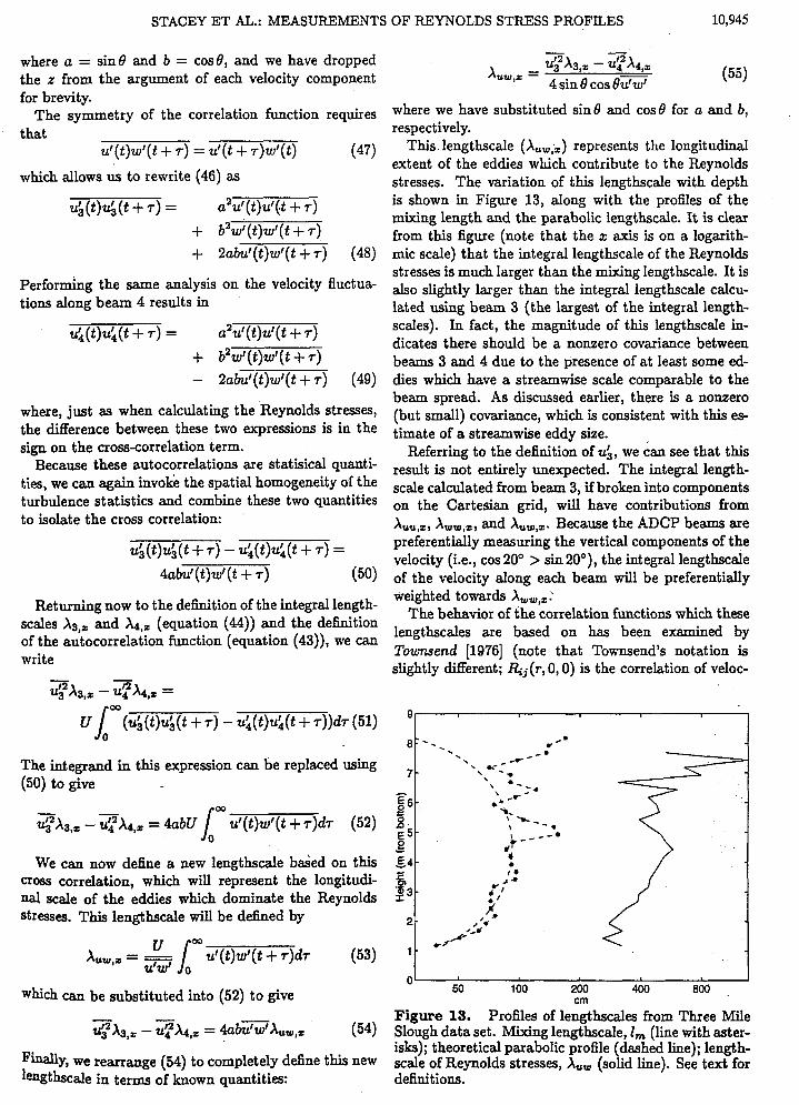
This lengthscale (Auw;z) represents the longitudinal extent of the eddies which contribute to the Reynolds stresses. The variation of this lengthscale with depth is shown in Figure 13, along with the profiles of the mixing length and the parabolic lengthscale. It is clear from this figure (note that the z axis is on a logarithmic scale) that the integral lengthscale of the Reynolds stresses is much larger than the mixing lengthscale. It is also slightly larger than the integral lengthscale calculated using beam 3 (the largest of the integral lengthscales). In fact, the magnitude of this lengthscale indicates there should be a nonzero covariance between beams 3 and 4 due to the presence of at least some eddies which have a streamwise scale comparable to the beam spread. As discussed earlier, there is a nonzero (but small) covariance, which is consistent with this estimate of a streamwise eddy size.

Referring to the definition of ui, we can see that this result is not entirely unexpected. The integral lengthscale calculated from beam 3, if broken into components on the Cartesian grid, will have contributions from A,,,,, Xww,21 and Xuur,z. Because the ADCP beams are preferentially measuring the vertical components of the velocity (i.e., cos2O0 > sin20°), the integral lengthscale of the velocity along each beam will be preferentially weighted towards XWw,,:

The behavior of the correlation functions which these lengthscales are based on has been examined by T o m e n d [1976] (note that Townsend’s notation is slightly different; &j(r, 0,O) is the correlation of veloc-

9

;? - - - - t I .

1 O‘ 50 100 200 400 800

cm Figure 13. Profiles of lengthscales from Three Mile Slough data set. Mixing lengthscale, I , (line with asterisks); theoretical parabolic profile (dashed line); lengthscale of Reynolds stresses, A,, (solid line). See text for definitions.


ity component i with component j in the x direction). For channel flow, Townsend tabulates the distance at which the correlation is reduced to 0.05; this distance is 6.8 times larger for Rll(r,O,O) than for R33(7-,0,0) (proportional to A,,,, in our notation). Therefore the longitudinal scales of velocity components which in- volve u’ (such as &,,) would be expected to be larger

s than those measured fiom the individual beams (such

These lengthscales have been estimated in a tidal boundary layer by Gross and Nowell [1985]. Using cur-

. rent meter triplets, estimates of Reynolds stress cospec- tra showed peaks at a wavelength of approximately 10 m, which are of the same order as the scales estimated here. Gross and Nowell also noted that this scale ex- ceeded the depth of their flow and argued that this sug- gested that the eddies which dominated the Reynolds stress measurements were “flattened out,” again consistent with the conclusions here.

We also note that the assumption that the largest turbulent eddies dominate the transfer of momentum is also supported by this distribution of the Reynolds stress length scale. Additionally, because the mixing lengthscale is meant to represent the vertical extent of the mixing events, the two scales together define the anisotropy of the eddies which dominate the vertical transport of momentum. From Figure 13, we estimate the horizontal scale to be 5-6 times larger than the vertical scale for the large eddies which are actively mixing the flow.

as As,,).

6. Application to Other Conditions The technique applied to this unstratified flow is a

powerful one, which holds a great deal of promise in the exploration of turbulent mixing in a variety of estuarine and coastal flows. However, in moving from an unstratified environment to a stratified one, additional factors need to be considered.

First of all, in stratified conditions, the stratification limits the size of the eddies to be less than the Ozmi- dov scale (lo= = ( E / N ~ ) ~ / ~ ) , which is analogous to the stratification lengthscale defined above (equation (42)). This places a limit on the ability of the ADCP to resolve turbulent motions due to the inherent averaging within each depth cell. Therefore an important consideration is the limit on the size of the eddies (which can be estimated by either the Ozmidov or stratification lengthscale) relative to the spatial average of the ADCP within each bin.

In addition to stratification imposing a limit on eddy size, presence of a boundary, such as the bed or the surface, wil l also constrain the size of the turbulent eddies. The effects of the ADCP bin size relative to this constraint may be evident in the near-surface region of the Three Mile Slough data set. In the upper meter of the water column, several quantities (particularly the lengthscales) exhibit huge variations in their mag-

nitudes. This is also the region where the lengthscale limitation of the surface would approach the bin size of the ADCP, resulting in a reduction in the ability to resolve the actual turbulent motions. In practice therefore the ability of an ADCP to resolve turbulent m& tions may be reduced in the near-bed and near-surface regions, depending on the bin size being used.

An additional effect of stratification is an increase in the anisotropy of the turbulence. Using the anisotropy values assumed here (equations (12a) and (12b), which are the unstratified values) will therefore introduce a bias into the calculation of q2. Because the ADCP measures a larger component of the vertical velocity than the horizontal, and stratification reduces the vertical motions, as anisotropy increases, our estimate of q2 will be below the actual value. The maximum error in these calculations has been estimated using the Holt et d., [1992] database and was found to be about 30% (see Stacey et al., [1999] for further discussion).

Finally, as was discussed above, boat motion, and the associated motion of the ADCP induces a variance in the data which could overwhelm the quantities being measured. The data from Three Mile Slough indicates that the bias in the turbulent kinetic energy may be most influenced by vertical translation of the sensor, rather than typical pitch and roll motions. However, pitch and roll motions will also induce variance into the measurements, in a manner proportional to equation (36). Therefore, it will be critical in making-these measurements that a stable platform be used which wil l minimize the effects of pitch, roll and vertical translation. Other successful ship-mounted measurements have been performed in estuarine flows (see Staced et al., 1999); in those cases, boat motion was completely negligible.

7. Conclusions Acoustic Doppler current profilers are beginning to be

used more and more widely in estuarine hydrodynamic studies. As a result , the teihnique presented here could be a valuable method for increasing the availability of information on turbulent mixing in stratified tidal flows.

The results from Three Mile Slough demonstrate that the noise levels associated with the ADCP are not p r e hibitively high when trying to resolve profiles of turbulence statistics. In fact, the agreement with theory was quite good in both the Reynolds stresses and the turbulent kinetic energy. Further, the errors that were seen in that data set, both in the biases and spreads, were consistent with those predicted by the application of statistical error analysis. The one exception was a potential downwards bias in the estimates of friction velocity based on the Reynolds stress profiles during the first hour of the deployment. This bias could have been due to either boat motion or the spatial averaging inherent in the ADCP system. If the downwards bias were due to the averaging of the ADCP, then during

STACEY E T AL.: MEASUREMENTS OF REYNOLDS STRESS PROFILES 10,947

the second hour of the data set, the friction velocity based on the Reynolds stresses would actually exceed that based on the mean velocities, a result which would be consistent with an increase in Reynolds stress activity during the deceleration phase of the tide.

The measurements in Three Mile Slough show a friction velocity which is somewhat higher than would be expected in'steady channel flow. However, high values of u. resulted from estimates using both logarithmic fits to the mean data and linear fits to the turbulence data. The logarithmic fits resulted in a roughness lengthscale of about 8.2 cm, which is suggestive of bed forms such as sand waves oriented across the channel. These bed forms would explain both the high values of U . and c d which were seen in the data.

The mixing lengthscale based on the Reynolds stress measurements and mean shear was parabolically dis- tributed, increasing away from the bed with very similar magnitude to the typically assumed parabolic profile. The distributions of additional integral lengthscales were also consistent with the mixing length, with magnitude approximately 2 times larger. This factor was consistent with the value from direct numerical simulation (DNS) of unstratified, sheared turbulence. Finally, the longitudinal lengthscale of the eddies which dominate the Reynolds stress measurements was found to be somewhat larger than the other lengthscales of the flow. This &ding reinforces the assumption that the largest eddies dominate the transport of momentum.

Based on these results in an unstratified channel, the variance technique presented here seems to hold promise in quantifying turbulent mixing over the entire water column of tidal flows. In stratified conditions [Stocey e t d., 19991 this technique allows for the simultaneous measurement of shear, stratification and turbulent mixing throughout the water column and tidal cycle. Such data sets will permit a much more in-depth examination of the balance of forces that determine the evolution of an estuarine water column.

Appendix: Error -Analysis Calculations In section 4.1.2 an important calculation was the vari-

ance of the quantity xi2, the square of the fluctuating component of the along-beam velocity measurements. In this appendix we give the details of the analysis which d h e s (29) .

First of all, the definition of variance allows us to write

(A21 E(#) = q + 0;

which can be substituted into ( A l ) to give

var (xi') = E[(U: + N)4 - 2 , 7 ( q + 0 N 2 ) _ . (ui2 + a N 2 ) 2 ] (A31

Evaluating the second and third terms gives

Var ($) = E[(u: + N)4] - (q + 0 ~ ' ) ' (A4)

The first term c& be expanded to give

E[(u: + N)4] = E[ui* + ~ u : ~ N + 6ufN2 + 4u:N3+N4] (A5)

We now note that the expected values of an odd power of a zero-mean Gaussian are zero, which requires E ( N ) = E ( N 3 ) = 0. Further, the fact that the noise is independent of the velocities requires that E[u$N2] = E(u:')E(N2) = $UN' so we can simplify (A5) to define

E[(u: + N ) 4 ] = E ( u ; ~ ) + 6 $ 0 ~ ' + E ( N 4 ) (A6)

Finally, if we define the kurtosis of the variables Q

and N .

we can substitute back into (A4) to give the variance of the measured velocities squared as

- var ( Z f ) = Ku,(ui2)2 + ~$UN' + K N U N ~ -

- (T)2 - 2u:2UN2 - ON (A81 This expression can be further simplified to

Var (x?) = (Kui - l)(T)' 4- 4$0N2 (KN - l)Ulv4 (A9)

which defines the quantity needed in the analysis of the variance in the turbulence estimates.

Notation

total along-channel velocity. total vertical velocity. total velocity along ADCP beam i. angle ADCP beam makes with the vertical. white noise random variable. friction velocity. coefficient of drag. total depth of the water column. vertical coordinate.


Z x’ P

< x > u, K, kurtosis of variable x.

Reynolds average (expected value) of variable x. fluctuations of variable x (x - Z). estimator of the mean of variable x. depth average of variable x. standard deviation of variable x.

surements and Experimentation, pp. 1-20, Am. SOC. Civ. Eng., New York, 1994.

Koseff, J. Re, J. K. Holen, S. G. Monismith, and J. E. Clo- ern, The effects of vertical mixing and benthic grazing on phytoplankton populations in shallow turbid estuaries, J. Mar. Res., 51, 1-26, 1993.

Kundu, P. K., Fluid Mechanics, Academic, San Diego, Calif., 1990.

Lai, C., Computational method of characteristics models

Acknowledgments. The authors wish to thank Mike Simpson of the USGS California District for his assistance in the data collection effort and technical expertise. The authors would also like to thank Jeffrey R. Koseff for his input

- on the analysis of lengthscales. This work was supported by NSF grant CTS8958314 and OCE9416604 to SGM who gratefully acknowledges NSF’s support. Additionally, fund- ing was provided by ONR grant N00014961-1292 during preparation of the manuscript. The authors also gratefully acknowledge the comments of two anonymous reviewers.

References Bendat, J. B. and A. G. Piersol Random Data: Analysis and

Measurement Procedures, John Wiley, New York, 1986. Bowden, K. F. and M. R. Howe, Observations of turbulence

in a tidal current, J. Fluid Mech., 17, 271-284, 1963. Burau J. R., M. R. Simpson, and R. T. Cheng, Tidal and

residual currents measured by an acoustic Doppler current profiler at the west end of Carquinez Strait, San Francisco Bay, California, March to November 1988, U.S. Geol. Sum. Water Resour. Invest. Rep., 92-4064, 1993.

Busch, N. E., Fluxes in the surface boundary layer over the sea, in Modelling and Prediction of the Upper Layers of the Ocean, edited by E. B. Kraus, pp. 72-91, Pergamon, Tarrytown, N.Y., 1977.

Dillon, T. M., Vertical overturns: A comparison of Thorpe and Ozmidov Length Scales, J . Geophys. Res., 87, 9601- 9613, 1982.

Dyer, F., The mixing processes in a partially mixed estuary: Southampton water, in Second International Symposium on Stmtijied Flows, vol. 2, edited by T. Carstens, and T. McClimans, pp.934-943, Tapir, Trondheim, Norway, 1980.

Efron, B., and R. J. Tibshirani, An Introduction to fhe Boot- stmp, 436 pp., Chapman and Hall, New York, 1993.

Farmer, D. and J. D. Smith, Tidal interaction of stratified flow with a sill in Knight Inlet, Deep Sea Res., 27A, 239- 254, 1980.

Gargett, A. E., Observing turbulence with a modified acoustic Doppler current profiler, J. Atmos. Oceanic Techno&,

Gargett, A. E. and J. N. Moum, Mixing efficiencies in tidal fronts: Results from direct and indirect measurements of density flux, J. Phys. Oceanogr., 25, 2583-2608,1995.

Geyer, W . R., Three-dimensional tidal flow around head- lands, J. Geophys. Res., 98, 955-966, 1993.

Gross, T. F. and A. R. M. Nowell, Spectral scaling in a tidal boundary layer, J. Phys. Oceancgr., 15, 496508, 1985.

Heathershaw, A. D. and J. H. Simpson, The sampling variability of the Reynolds stress and its relation to boundary shear stress and drag coe5cient measurements, Estuarine Coastal Mar. Sci., 6, 263-274, 1978.

Holt, S. E., J. R. Koseff, and J. H. Ferziger, The evolution of turbulence in the presence of mean shear and stable stratification, J . Fluid Mech. , 237, 499-539, 1992.

Imberger, J. and R. Head, Measurement of turbulent p r o p erties in natural system, in Proceedings of the Symposium on Fundamentals and Advancements in Hydmulic Mea-

11, 1592-1610,1994.

for flow simulation, J. Hydmul. Eng., 144(9), 10741097, 1988.

Lehfeldt, R., and S. Bloss, Algebraic turbulence model for stratified tidal flows, in Physical Processes in Estuaries, edited by J. Dronkers and W. van Leussen, pp. 278291, Springer-Verlag, New York, 1988.

Lohrmann, A., B. Hackett, and L. D. Roed, High resolution measurements of turbulence, velocity, and stress using a pulse-to-pulse coherent sonar, J. Atmos. Oceanic Tech- nol., 7, 1437, 1990.

Lu, Y., Flow and turbulence in a tidal channel, Ph.D. thesis, 140 pp., University of Victoria, Victoria, B.C., 1997.

Lueck, R. G., and Y. Lu, The logarithmic layer in a tidal channel, Cont. Shelf Res., 17(14), 1785-1801, 1997.

Mellor, G. L., and T. Yamada, Development of a turbulence closure model for geophysical fluid problems, Rev. Geo-

Nezu, I., and H. Nakagawa, nrbulence in Open Channel Flows, A. A. Balkema, Brookiield, Vt., 1993.

Nunes-Vaz, R. A., and J. H. Simpson, lhrbulence closure modeling of estuarine stratification, J. Geophys. Res. , 99,

Peters, H., Observations of stratified turbulent mixing in an estuary: Neap-to-spring variations during high river flow, Estuarine CooJtal Shelf Sci., 45, 69-88, 1997.

Plueddemann, A. J., Observations of the upper ocean using a multi-beam Doppler sonar, Ph.D. thesis, Univ. of Calif., San Diego, La Jolla, 1987.

RD Instruments, Direct-Reading and Self-Contained B m d - band Acoustic Doppler Current Profiler Technical Manual, San Diego, Calif., 1995.

Schroder, M., and G. Siedler, Turbulent momentum and salt transport in the mixing zone of the elbe estuary, Estuarine Coastal Shelf Sci., 28, 615-638, 1989.

Seim, H. E., and M. C. Grenn, Energetics of a naturally

phys., 20, 851-875, 1982.

16143-16160, 1994.

occurring shear instability, 7‘ Geopigs. Res., 100, 4943- 4958, 1995.

Shanmugan, K. S., and A. M. Breipohl, Random Signals: Detection, Estimation, and Data Analysis, John Wiley, New York, 1988.

Soulsby, R. L., Selecting record lengths and digitization rate for near-bed turbulence measurements, J. Phys. Oceanogr. , 10, 208-219, 1980.

Stacey, M. T., Turbulent mixing and residual circulation in a partially stratified estuary, Ph.D. thesis, 209 pp., Stanford

. Univ., Stanford, Calif., 1996. Stacey, M. T., S. G. Monismith, and J. R. Burau, Obser-

vations of turbulence in a partially stratified estuary, J. Phys. Oceanogr., in press, 1999.

Tennekes, H., and J. L. Lumley, A First Course in ILrbu- lence, 300 pp., MIT Press, Cambridge, Mass., 2972.

Townsend, A. A. The Structure of Ihrrbulent Shear Flow, 429 pp., Cambridge University Press, New York, 1976.

nopea, C., A note concerning the use of a one-component LDA to measure shear stress terms, Ezp. in Fluids, I, 10, 209-210,1981.

van Haren, H., N. Oakey, and C. Garrett, Measurements of internal wave band eddy fluxes above a sloping bottom, J. Mar. Res., 52, 909-946, 1994.


J. R Burau, United States Geological Survey, Placer Hall, M. T. Stacey, Department of Integrative Biology, VLSB 6000 J Street, Sacramento, CA 958146129. (e-mail: bu- 3060, University of California, Berkeley, Berkeley, CA [email protected]) 94720.3140. (email: mstacey9socrates.berkeley.edu) S. G. Monismith, Civil Engineering Department, Stan-

ford University, Stanford, CA 94305-4020. (e-mail: manis- mitQce.stauford.edu) accepted September 21, 1998.)

(Received JdY 181 1997; revised JdY 15, 1998;

,

measurements of reynolds stress profiles in unstratified … · · 2005-09-01measurements of...

Documents