measures of post-processing the human body response to transient fields

MEASURES OF MEASURES OF POST-PROCESSING POST-PROCESSING

THE HUMAN BODY RESPONSE THE HUMAN BODY RESPONSE TO TRANSIENT FIELDSTO TRANSIENT FIELDS

Dragan PoljakDragan PoljakDepartment of Electronics, University of Department of Electronics, University of

SplitSplitR.Boskovica bb, 21000 Split, CroatiaR.Boskovica bb, 21000 Split, Croatia

Email: Email: [email protected]@fesb.hrThe scope:

The calculation procedures for some meausures to evaluate human response to transient electromagnetic radiation.

CONTENTSCONTENTS

IntroductionIntroduction Time Domain Representation of the Time Domain Representation of the

BodyBody Some Measures for the Body Some Measures for the Body

Transient ResponseTransient Response Computational ExamplesComputational Examples ConclusionConclusion

1 Introduction1 Introduction

The transient current induced inside the body is The transient current induced inside the body is the key parameter in the analysis of the the key parameter in the analysis of the interaction of human beings with transient fields.interaction of human beings with transient fields.

Transient exposures can be analyzed using the Transient exposures can be analyzed using the

human equivalent antenna modelhuman equivalent antenna model ( (Poljak, Tham, Poljak, Tham, Sarolic, GandhiSarolic, Gandhi IEEE Trans EMC Feb 2003). IEEE Trans EMC Feb 2003).

Once obtaining the transient response of the Once obtaining the transient response of the body it is possible to compute certain parameters body it is possible to compute certain parameters providing a measure of the transient current. providing a measure of the transient current.

2 Time Domain Model of2 Time Domain Model of the the Human Human BodyBody

The time domain study of the EMP coupling to the body is based on a cylindrical body representation (L=1.8m, a=5cm)

Fig 1 The human body exposed to transient radiation

2 T2 Time Domain Model ime Domain Model (cont’d)(cont’d)

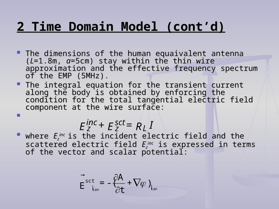
The dimensions of the human equaivalent antenna The dimensions of the human equaivalent antenna ((LL=1.8m, =1.8m, aa=5cm) stay within the thin wire approximation =5cm) stay within the thin wire approximation and the effective frequency spectrum of the EMP (5MHz).and the effective frequency spectrum of the EMP (5MHz).

The integral equation for the transient current along the The integral equation for the transient current along the body is obtained by enforcing the condition for the total body is obtained by enforcing the condition for the total tangential electric field component at the wire surface:tangential electric field component at the wire surface:

where where EEzzincinc is the incident electric field and the scattered is the incident electric field and the scattered

electric field electric field EEzzincinc is expressed in terms of the vector and is expressed in terms of the vector and

scalar potential:scalar potential:

IR=E+E Lsctz

incz

)+t

A-(=E |

sct| tantan

2 2 Time Domain Model Time Domain Model (cont’d)(cont’d)

where the vector potential is defined by:where the vector potential is defined by:

and the scalar potential is given by:and the scalar potential is given by:

where where ρρss and and JJ are space-time dependent surface are space-time dependent surface charge and surface current density.charge and surface current density.

'

,,

dSR

R/c)-t,r(J

4=A

S

'

,,

dSR

R/c)-t,r

S

(

4

1=

2 2 Time Domain Model Time Domain Model (cont’d)(cont’d)

They are related with the continuity equation:They are related with the continuity equation:

and and RRLL is the resistance per unit length of the is the resistance per unit length of the antenna length:antenna length:

t-=J

ss

2

1

aRL

The integral equation for the transient current along the body is given by:

Integrating the Pocklington equation yields the Hallen integral equation:

-I(z,, t-R/c) is the unknown current to be determined, - c is the velocity of light, -Z0 is the wave impedance of a free space

-F0(t); FL(t) are related with the current reflections from wire ends -R is the resistance per unit length of the antenna length

t

I(z,t)R-dz

R4

R/c)-,tz(I

tc

1-

z=

tE- L

,,L

2

2

2

2incz

0

'|'|

,'()'(2

1')

|'|,'(

2

1

0000

dzc

zztzIzR

Zdz

c

zztz

Z

+)c

z-L-(tF+)

c

z-(tF=dz

R4R/c)-t,zI(

L

L

Lincz

L0,

,L

0

E

The time domain Hallen equation is solved via the Galerkin-Bubnov indirect boundary element approach.

3 The Boundary 3 The Boundary EElement Solution of the lement Solution of the Hallen Hallen IIntegral ntegral EEquationquation The The Hallen Hallen integral equation can be written in the integral equation can be written in the

operator form:operator form:

- - LL is linear integral operator, is linear integral operator, - I- I is the unknown function to be determined for a given is the unknown function to be determined for a given

excitation Yexcitation Y

The unknown solution for current is given in the form of The unknown solution for current is given in the form of linear combination of the basis functions:linear combination of the basis functions:

{f} is the vector containing the basis functions {f} is the vector containing the basis functions {I} is the vector containing unknown time dependent {I} is the vector containing unknown time dependent

coefficients of the solution. coefficients of the solution.

Y=L(I)

{I} }{f=)tI(z T','

3 3 The Boundary The Boundary EElement Solutionlement Solution (cont’d)(cont’d)

The request for minimization of the interpolation The request for minimization of the interpolation error error

yields:yields:

Applying the boundary element algorithm the Applying the boundary element algorithm the local matrix system for i-th source element local matrix system for i-th source element interacting with interacting with

j-th observation element is given as follows:j-th observation element is given as follows:

1,2,...N=j 0,=dzWY]-[L(I)L

j0

dzdzffzRZ

dz ){fc

|-z|-t,(

2

1+dz ){f

c

z-L-(t

+dz ){fc

z-(t

Tij

jl

il

L

dz}z

zE Z

}F

}F}{Idz dzR4

1}{f }{f

,j

,,inc

z

ll0jL

l

j0

l|

,Tij

ll

ijj

jR/c-t

ij

')'(2

1

0


The calculation procedure is more efficient if the The calculation procedure is more efficient if the known excitation is also interpolated over wire known excitation is also interpolated over wire segment:segment:

where {E} is the time dependent vector where {E} is the time dependent vector

containing known values of the transient containing known values of the transient excitation. excitation.

Hence, the matrix equation becomes:Hence, the matrix equation becomes:

{E}}{f=)t,z(ET,,inc

z

c

zzt

j i

c

|z ,-z|-t

ij

j

jc

R-t

ij

IdzdzffzRZ

}{Edz dz}{f }{f Z2

1+

+dz }){fc

z-L-(tF

}F= }{Idz dzR4

1}{f }{f

Tij

l lL

|,T

ijll0

jLl

j0

l|

,Tij

ll

+dz ){fc

z-(t

|'||')'(2

1


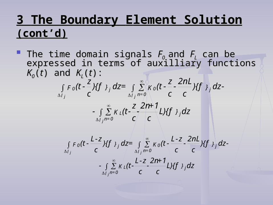
The time domain signals The time domain signals FF00 and and FFLL can be can be expressed in terms of auxilliary functions expressed in terms of auxilliary functions KK00((tt) ) and and KKLL((tt):):

dzL){fc

1+2n-

c

z-(t-

-dz){fc

2nL-

c

z-(t=dz ){f

c

z-(t

}K

}K}F

jL0=nl

j00=nl

j0

l

j

jj

dzL){fc

1+2n-

c

z-L-(t-

-dz){fc

2nL-

c

z-L-(t=dz ){f

c

z-L-(t

}K

}K}F

jL0=nl

j00=nl

j0

l

j

jj


defined by relations:defined by relations:

aandnd

}{Izd}{fzRZ2

1

}{Ezd}{fZ2

1 - }{I dz

R4

1}{f=(t)K

|,T

iLl0

|,T

il0

|,

0

Ti

l0

cz ,

-ti

cz ,

-tic

R0-ti

)'(

}{Izd}{fzRZ2

1

}{Ezd}{fZ2

1 - }{I dz

R4

1}{f=(t)K

|,T

iLl0

|,T

il0

|,

L

Ti

lL

cz ,-L

-ti

cz ,-L

-tic

R L-ti

)'(


The rearranging of the matrix equation yields:The rearranging of the matrix equation yields:

I[R]

E[B]+

+I[C]-

I[R]

E[B]-

-I[D]+

IR

E[B]+

+I[D]-

I[R]

E[B]-

-I[C]+

}[B]{E=}[A]{I

n=0n |

n=0n |

n=0n |

n=0n |

n=0n |

n=0n |

n=0n |

n=0n |

n=0n |

n=0n |

n=0n |

n=0n |

||

cz,

-Lc

1+2n-

c

z-L-t

cz,

-Lc

1+2n-

c

z-L-t

cR0-L

c

1+2n-

c

z-L-t

cx,-L

-c

2nL-

c

z-L-t

cx,-L

-c

2nL-

c

z-L-t

cRL-

c

2nL-

c

z-L-t

cz,-L

-Lc

1+2n-

c

z-t

cz,-L

-Lc

1+2n-

c

z-t

cRL-L

c

1+2n-

c

z-t

cz,

-c

2nL-

c

z-t

cz,

-c

2nL-

c

z-t

cR0-

c

2nL-

c

z-t

c

|z,-z|-t

c

R-t

][


The interaction matrices [A], [C] and [D] are of the form:The interaction matrices [A], [C] and [D] are of the form:

where G(z,z,) is the corresponding Green function. where G(z,z,) is the corresponding Green function.

[B] matrix is given by expression: [B] matrix is given by expression:

and the resistance matrix is of the form:and the resistance matrix is of the form:

The matrix system (19) can be, for convenience, written in the form: The matrix system (19) can be, for convenience, written in the form: (23)(23) where where gg is the space-time dependent vector representing the entire right hand side of the matrix equation (20). is the space-time dependent vector representing the entire right hand side of the matrix equation (20). The solution in time for unknown current coefficients is given by: The solution in time for unknown current coefficients is given by: (24)(24) where where NTNT is the total number of time segments. is the total number of time segments. The weighted residual approach for the time increment yields:The weighted residual approach for the time increment yields: (25)(25)

NtNt is the total number of time samples, is the total number of time samples, θk denotes the set of time domain test functions.θk denotes the set of time domain test functions.

Choosing the Dirac impulses as test functions it follows:Choosing the Dirac impulses as test functions it follows: (26)(26) The space-time discretisation condition is given by: The space-time discretisation condition is given by: (27)(27) The resulting recurrence formula for the space-time dependent current is of the form: The resulting recurrence formula for the space-time dependent current is of the form: (28)(28)

Ng is the total number of space nodes, Ng is the total number of space nodes, the horizontal line over matrix [A] denotes the absence of diagonal terms.the horizontal line over matrix [A] denotes the absence of diagonal terms.

The appropriate boundary conditions at the wire ends are:The appropriate boundary conditions at the wire ends are: (29)(29) The initial condition to be satisfied over the entire length of the wire at t=0 is:The initial condition to be satisfied over the entire length of the wire at t=0 is: (30)(30) Now, everything is ready to start the stepping procedure. Now, everything is ready to start the stepping procedure.

dzzd}{f}){fzG(z,= ,Tij

,

ll ij

dzzd}{f}{fZ2

1=B ,T

ijll0 ij

dzzd}{f}{fzRZ2

1=R ,T

ij

ll0L

ij

)'(


The matrix system can be, for convenience, written in the form: The matrix system can be, for convenience, written in the form:

where where gg is the space-time dependent vector representing the entire is the space-time dependent vector representing the entire right hand side of the matrix equation.right hand side of the matrix equation.

The solution in time for unknown current coefficients is given by: The solution in time for unknown current coefficients is given by:

where where NNTT is the total number of time segments. is the total number of time segments. The weighted residual approach for the time increment yields:The weighted residual approach for the time increment yields:

θk denotes the set of time domain test functions.θk denotes the set of time domain test functions.

g=}{IA |c

R-t

)t(TI=)t(I ,kki

N

1=k

,i

t

N1,2,...,=k 0,=dt{g})-}([A]{I Tk|

t+t

tR/c-t

k

k

3 3 The Boundary element SolutionThe Boundary element Solution (cont’d)(cont’d)

Choosing the Dirac impulses as test functions it follows:Choosing the Dirac impulses as test functions it follows:

The space-time discretisation condition is given by: The space-time discretisation condition is given by:

The resulting recurrence formula for the space-time The resulting recurrence formula for the space-time dependent current is of the form: dependent current is of the form:

Ng is the total number of space nodes, the horizontal line over Ng is the total number of space nodes, the horizontal line over matrix [A] denotes the absence of diagonal terms.matrix [A] denotes the absence of diagonal terms.

}{g=}[A]{I || instants previous discrete allR/c-tk

c

zt

N1,2,...,=k ,N1,2,...,=j

,a

g+I a-

=I

Tg

jj

jiji

N

1=ij

| instants previous discrete all| R/c-tk

g

|tk


The appropriate boundary conditions at the wire The appropriate boundary conditions at the wire ends are:ends are:

The initial condition to be satisfied over the entire The initial condition to be satisfied over the entire

length of the wire at t=0 is:length of the wire at t=0 is:

Now, everything is ready to start the stepping Now, everything is ready to start the stepping procedure. procedure.

0=t)I(L,=t)I(0,

0=I(z,0)

4 Measures of a transient response ° average value of the transient current ° root-mean-square value of the transient current ° instantaneous power ° average power ° total absorbed energy ° specific absorption 4.1 Average value of a transient current The average value of a time varying current i(t) is defined as:

where T0 is the period of the waveform.

0

00)(

1 T

av dttiT

I

When the current along the wire at each node and time instant is known, Iav(x) is simply given by:

and the performing of a straight-forward integration yields:

where {T} is the vector containing the time domain linear shape functions.

The distribution of average values of current is simply given by:

0

00),(

1)(

T

av dttxiT

xI

dt){I}}({TT

I iT

t

t

N

1=k0av

1+k

k

t

1

])I(+)I[(T

t=I 1+k

iki

N

1=k0rms

t

2

while the corresponding average power Pav is determined by the integral relation:

from which the rms current is then:

4.2 Root-Mean-Square measure for a transient response Instantaneous power delivered to a resistance RL by a transient current i(t) is:

(t)iR=p(t) L2

IR = (t)dtiRT

1dttp

T=P 2

rmsL2

L

T

00

T

av

0

0

00)(

1

(t)dtiT

1=I 2

T

00rms

0

where T0 is the time interval of interest. When the current along the wire at each node and time instant is known, the rms value of the wire current can be computed from the following relation:

The rms value of the thin wire space-time current distribution is given by:

t)dt(x,iT

1=(x)I 2

T

00rms

0

dt){I}}({TT

1=I

2i

Tt

t

N

1=k0rms

1+k

k

t

where σ is the average conductivity and S is the cross-section of the body

and the performing of a straight-forward integration yields:

where {T} is the vector containing the time domain linear shape functions.

4.3 Instantaneous power

Instantaneous power is defined by integral:

])I(+II+)I[(T

t=I

21+ki

1+ki

ki

2ki

N

1=k0

rms

t

3

dztziS

L

),(1

0

2 dVtrEtp

V

rad ,)(2

The BEM solution for instantaneous power is given by:The BEM solution for instantaneous power is given by:

where where II is the current at i-th node and k-th instant. is the current at i-th node and k-th instant.

M

i

ki

ki

ki

ki

M

i

L

l

i

T

irad

IIIIz

S

dzIfS

tpi

1

2

11

2

1

2

3

1

1)(

4.4 Average power

The average absorbed power is defined as:

L t

t Lt

radav

dzdttzitS

dtdztziSt

dttpt

P

0 0

2

0 0

2

0

),(11

),(11

)(1

And can be written in the form:And can be written in the form:

L

rmsav dzzIS

P0

2 )(1

M

i

kirms

kirms

kirms

kirms

M

i

L

l

irms

T

iav

IIIIz

S

dzIfS

Pi

1

2

1,1,,

2

,

1

2

3

1

1

where Irms is the effective value of the current.

The BEM solution can be written as follows:

4.5 Absorbed power 4.5 Absorbed power

The total absorbed energy can be obtained integrating The total absorbed energy can be obtained integrating the instantaneous power:the instantaneous power:

tPdttptW av

t

radtot 0

)()(

The BEM solution is given by:

t

t k

k

N

k

kk

N

k

tt

tk

Tktot

PPt

dtPTtW

1

1

1

2

)(

4.6 Specific Absorption4.6 Specific Absorption

The BEM solution is given as follows:The BEM solution is given as follows:

)(),(1 2

0

2 zIS

Tdttzi

S rms

T

The specific absorption rate can be defined as:

M

i

ki

ki

ki

ki

N

k

tt

tk

Tk

IIIIt

S

dtITS

SAT k

k

1

21

12

1

2

31

1

tt

dtE

SARdtSA00

5 Computational examples

Gaussian pulseGaussian pulse unit step functionunit step function EMP waveformEMP waveform

Types of excitation considered:

5.1 Gaussian pulse

20

2 )(0)( ttgeEtE

Fig 2: Transient current induced in the human body exposed to theGaussian pulse waveform

with: with: EE00=1V=1V//m, g=2*10m, g=2*1099, , tt00==2ns2ns..

5.1.1 Spatial distribution of the average and rms values along the body for the Gaussian pulse exposure

Fig 3: Average value of current Fig 4: RMS value of current

5.1.2 Instantaneous power and absorbed energy versus time for the Gaussian pulse exposure

Fig 5: Instantaneous power Fig 6: Absorbed energy

5.2 Step function

)()( 0 tuEtE

where u(t) denotes the unit step

Fig 7: Transient current induced in the human body exposed to thestep function waveform

5.2.1 Spatial distribution of the average and rms values along the body for the step function exposure


5.2.2 Instantaneous power and absorbed energy versus time for the step function exposure


5.3 Electromagnetic pulse (EMP)

with with EE00=1.05V=1.05V//m, m, aa=4*10=4*1066ss-1-1, , bb=4.76*10=4.76*108 8 ss-1-1. .

)()( 0btat eeEtE

Fig 12: Transient current induced in the human body exposed to theEMP waveform

5.3.1 Spatial distribution of the average and rms values along the body for the step function exposure


5.3.2 Instantaneous power and absorbed energy versus time for the step function exposure


66 Conclusion Conclusion

The exposure of human body to transient electromagnetic fields The exposure of human body to transient electromagnetic fields is analysed in this work.is analysed in this work.

Time domain Time domain formulationformulation is based on the is based on the human equivalent human equivalent antennaantenna representation of the body representation of the body

Some useful measures for the analysis of the body transient Some useful measures for the analysis of the body transient response are proposedresponse are proposed::

° ° average average valuevalue of the transient current of the transient current ° ° rroot-mean-squareoot-mean-square value value of the of the transient transient currentcurrent ° ° instantaneous powerinstantaneous power ° ° average poweraverage power ° ° total absorbed energytotal absorbed energy ° ° specific absorptionspecific absorption

TThe related numerical results are presented.he related numerical results are presented.

measures of post-processing the human body response to transient fields

Documents

human body response

time domain hallen equation

transient exposures

unknown current

time domain model contdthey

time domain model contdwhere

human response

current reflections