measuring 30-day mortality following hospitalisation · 2017-04-11 · spotlight on measurement...
TRANSCRIPT

Measuring 30-day mortality following hospitalisation2nd edition
Spotlight on Measurement

BUREAU OF HEALTH INFORMATION
Level 11, 67 Albert Avenue Chatswood NSW 2067 Australia Telephone: +61 2 9464 4444 Email: [email protected] bhi.nsw.gov.au
© Copyright Bureau of Health Information 2017 This work is copyrighted. It may be reproduced in whole or in part for study or training purposes subject to the inclusion of an acknowledgement of the source. It may not be reproduced for commercial usage or sale. Reproduction for purposes other than those indicated above requires written permission from the Bureau of Health Information.
State Health Publication Number: (BHI) 170152 ISBN 978-1-76000-261-9 ISSN: 2204-1598 (Print), 2204-552X (Online)
Suggested citation: Bureau of Health Information. Spotlight on Measurement: Measuring 30-day mortality following hospitalisation. Sydney (NSW): BHI, 2017.
Please note there is the potential for minor revisions of data in this report. Please check the online version at bhi.nsw.gov.au for any amendments.
Published April 2017
The conclusions in this report are those of BHI and no official endorsement by the NSW Minister for Health, the NSW Ministry of Health or any other NSW public health organisation is intended or should be inferred.

Spotlight on Measurement: Measuring 30-day mortality following hospitalisation bhi.nsw.gov.au
Table of contents
Foreword 2
Summary 3
Setting the scene 6
Introduction 7
1. Relevance and validity 14
Why report mortality? 15 Including or excluding private hospital patients 17 Coding of transfers between hospitals 19 Association between outcomes and processes 21 Ischaemic stroke severity and transient ischaemic attack 23 Hip fracture surgery at first hospital 25 Presentation to an emergency department prior to admission 27 Transfer on the first day of admission 29 Palliative care admissions 31
2. Sensitivity and specificity 34
Implications of one-, two-, or three-year measurement periods 35 The effect of different measurement periods 37 Varying funnel plot control limits 39 Assessing mortality in small hospitals 41 Describing acute myocardial infarction 43 ‘Unspecified AMI’ and adjusting for STEMI status 45 Adjusting for socioeconomic status 47 Exploring partner hospital performance 49 Adjusting for history and frequency of hospitalisations for COPD and CHF 51 Random or last period of care 53 Depth of diagnosis coding 55
3. Actionability and timeliness 58
Using rolling time periods 59 Using linked or unlinked data 61 Relying on ‘fact of death’ or ‘cause of death’ information 63 Comparing RSMRs and unadjusted mortality rates 65 Hospital results – RSMRs and unadjusted rates 67
Conclusion 69
Appendices 72
References 111
Glossary 114
Acknowledgements 115

1 Spotlight on Measurement: Measuring 30-day mortality following hospitalisation bhi.nsw.gov.au

2Spotlight on Measurement: Measuring 30-day mortality following hospitalisation bhi.nsw.gov.au
At face value, mortality is one of the most easily understood outcomes of healthcare. Unlike many other constructs – such as quality of life or functional status – death is unambiguous, clearly defined and universally resonant for patients, clinicians and managers.
Measures of mortality are however, powerful indicators to be applied judiciously. Influenced by factors such as clinical processes, organisational capacity and integration of care, mortality indicators reflect a broad range of quality issues and can help assess healthcare performance at both a system and hospital level.
Importantly, although death is always a meaningful event, every death is not a direct reflection of performance. Many deaths are unavoidable, and may even be an expected outcome in some circumstances. Differences in mortality across hospitals that persist after adjusting for patient-level factors and case mix can however be a reflection of unwarranted clinical variation.
In 2013, the Bureau of Health Information released a report — 30-day mortality following hospitalisation, five clinical conditions, NSW, July 2009 – June 2012 — which used a risk-standardised mortality ratio (RSMR) to assess the presence of such variation. The report emphasised that RSMRs cannot, in isolation, provide unequivocal evidence of either good or poor performance. Most useful as a form of screening tool, they help identify where further assessment of performance may be needed and where improvement efforts could be focused.
This edition of Spotlight on Measurement builds on previous reports which described the analytic steps taken to develop and validate the RSMR for application in a NSW context; and to establish a reporting frequency regime. It features previously published sensitivity analyses on the validity of the RSMR, and supplements them with new analyses that explore a range of contextual issues and externalities.
These new analyses look at differences across hospitals in palliative care coding, in the depth of coding of secondary diagnoses in patient records, and in the propensity to perform surgery among patients admitted with a hip fracture. They also examine a number of attribution questions including whether considering patient visits to an emergency department in the 24 hours preceding the index hospitalisation affect hospital results, and the impact of including a randomly selected period of care, rather than the last period of care for each patient.
All of these new analyses seek to ensure that mortality measures are used with an understanding of the impact that contextual factors have on results. By being transparent about these implications, we hope to ensure RSMRs are used appropriately – reflecting on performance and identifying areas where further, more local investigation into variation in patient care may be required.
Jean-Frédéric Lévesque MD, PhD Chief Executive, Bureau of Health Information
Foreword

3 Spotlight on Measurement: Measuring 30-day mortality following hospitalisation bhi.nsw.gov.au
This report builds on previous publications that described the development of a risk-standardised mortality ratio (RSMR) suitable for public reporting of hospital performance.1-3 This edition updates previously published sensitivity and validation studies and presents new analyses undertaken in support of a release of new mortality results for the period July 2012 – June 2015.4
This revised edition of Spotlight on Measurement retains the structure of the version released in 2015. Data from original sensitivity analyses relate primarily to 2009–12 while newer analyses are based on 2012–15 data. The conclusions from these analyses are presented in terms of relevance and validity; sensitivity and specificity; actionability and timeliness.
Relevance and validity
Mortality reporting can play a key role in assessing healthcare performance, providing accountability, and targeting and guiding improvement efforts. Implications of using the RSMR approach in the mixed hospital sector of NSW were assessed by comparing inclusion and exclusion of private hospital patients in the predictive models and RSMR calculations, with a very minor impact on results.
The validity of the RSMR was assessed in terms of:
• Inconsistencies in coding of patient transfers and discharges – there were a small number of patient transfers miscoded as discharges; recodes did not however substantively change the results
• The prevalence and distribution of palliative care type codes in patients’ hospital records with a one-year lookback – in each of the conditions of interest, less than 1% of patients admitted for an acute hospitalisation had a history of a palliative hospitalisation in the previous year
• Whether attribution of results to an admitting hospital was substantively affected by patients attending another hospital emergency
department (ED) in the preceding 24 hours, or by patterns of transfers on the first day of hospitalisation – there was no clear relationship between rates of these events and outlier status
• Variation in the percentage of hip fracture surgery patients who were first admitted to another hospital – there was no clear association between hospital rates and outlier status
• Whether there was evidence of misdiagnosis of transient ischaemic attack as ischaemic stroke – merging these conditions and re-running analyses did not substantially alter the results.
The validity of the RSMR is supported by an independent audit of ischaemic stroke care conducted by the NSW Agency for Clinical Innovation (ACI). The audit found broad concordance between the RSMR-derived hospital outlier status and audit-based process measures of quality of care.
Sensitivity and specificity
Using a three-year rather than a one-year measurement period increased the number of hospitals reaching the reporting threshold (50 patients) by 13% for hip fracture surgery, 17% for pneumonia, 40% for acute myocardial infarction, 41% for ischaemic stroke, and 167% for haemorrhagic stroke.
Investigations into the ability of the RSMR approach to identify sustained levels of high ratios which do not reach statistical significance (particularly in smaller hospitals) found that an RSMR threshold of 1.5 identifies patterns of performance that may warrant further investigation.
Analyses that assessed the impact of adjusting for socioeconomic status found little improvement in the predictive power of the models and few meaningful changes to outlier results. Adjusting for the time elapsed since first diagnosis of a chronic condition, in addition to the number of recent admissions for the condition, did not improve the model and had little impact on RSMRs.
Summary

4Spotlight on Measurement: Measuring 30-day mortality following hospitalisation bhi.nsw.gov.au
The distribution of cause of death was similar for deaths both in-hospital and after discharge
Examining hospital RSMRs (observed mortality/ expected mortality) over time showed that observed rates varied more than expected rates. This suggests the characteristics of patients presenting to each hospital did not change markedly across measurement periods, but that observed mortality was more variable.
Looking across five conditions, there was generally a good correlation between the RSMR and the observed unadjusted mortality rate.
Assessing the impact of selecting, for patients with multiple periods of care in the study period, a random rather than the last period of care decreased the number of deaths captured. Using a random period of care had a small impact on most hospital results, changing RSMRs on average, by 0.07.
Variation and changes over time in the depth of secondary diagnosis coding was assessed as a source of potential bias. Across NSW, the average number of secondary diagnoses has increased. A few hospitals have patterns of secondary diagnosis coding that differ substantively from the NSW average and their RSMRs should be assessed alongside unadjusted and age-sex standardised results.
Actionability and timeliness
Rolling RSMRs (where measurement periods form a series of overlapping time intervals) are more likely to capture short-term variations in hospital performance compared to discrete measures of the same length. Temporary but marked fluctuations in performance can continue to influence rolling RSMRs for several periods — unlike RSMRs based on discrete periods.
There is a trade-off between the timeliness of reporting and the level of detail it is possible to provide. Across five conditions, between 21% and 50% of deaths occurred after discharge. Using linked patient data captures deaths after discharge. A comparison of unlinked data (which are available after a six-week lag) and linked data (which are available after a seven-month lag) in the construction of funnel plots for ischaemic stroke found that 15 hospitals changed outlier status. Therefore the use of linked data provided more robust and meaningful RSMRs and incurred only a modest trade-off in terms of timeliness of data.
There is limited benefit however in waiting two and a half years for ‘cause of death’ data to become available. The majority of deaths are attributed to the condition for which patients were hospitalised.
The utility of the RSMR as a meaningful measure of healthcare performance is well established, both internationally and in a NSW context. The RSMR is based on statistical analyses that take account of patient characteristics and hospital case mix.
The results of the analyses in this edition of Spotlight on Measurement indicate that for 30-day mortality reporting, a mix of different approaches is useful. The results support using:
• RSMRs to make fair assessments of hospital performance and reflect differences in the care provided. Such risk-standardised analyses can be time consuming, but are preferred for summative performance assessment and reporting.
• Unadjusted mortality rates — which can be produced in a more timely way — to provide formative assessments of performance to local providers within the NSW healthcare system.

5 Spotlight on Measurement: Measuring 30-day mortality following hospitalisation bhi.nsw.gov.au

6Spotlight on Measurement: Measuring 30-day mortality following hospitalisation bhi.nsw.gov.au
Setting the scene

7 Spotlight on Measurement: Measuring 30-day mortality following hospitalisation bhi.nsw.gov.au
In December 2013, BHI published 30-day mortality following hospitalisation, five clinical conditions, NSW, July 2009 – June 2012 that focused on acute myocardial infarction (AMI), ischaemic stroke, haemorrhagic stroke, pneumonia and hip fracture surgery. BHI have now updated this report for the July 2012 – June 2015 period and included two additional conditions – congestive heart failure (CHF) and chronic obstructive pulmonary disease (COPD).
Performance is measured for all hospitals (with at least one expected death) but only peer group* A-C hospitals with at least 50 patients for a condition are named in public reports. The number and type of hospitals included in the most recent three year reporting period, July 2012 to June 2015, and the distribution of patients is shown in Figure 1.
BHI assesses hospital performance in 30-day mortality outcomes using a risk-standardised mortality ratio (RSMR). RSMRs compare for each hospital the number of deaths that occurred (in or out of hospital) within 30 days of admission with the ‘expected’ number of deaths. The ‘expected’ number of deaths is generated by a statistical model that takes into account patient characteristics that affect the likelihood of dying following hospitalisation.
RSMRs less than 1.0 indicate lower than expected mortality, and greater than 1.0, higher than expected mortality. Small deviations from 1.0 are not meaningful. Funnel plots are used to determine whether the observed mortality is significantly different from expected. The 2013 report on 30-day mortality featured funnel plots with control limits set at 90% and 95%. In line with international best practice and in order to enhance specificity and limit the chance of making type I errors, new analyses in this report based on the period July 2012 to June 2015 use funnel plots with more stringent 95% and 99.8% control limits. The other analyses in this report based on the period July 2009 to June 2012 have funnel plots with 90% and 95% control limits.
As with any statistic, caution is needed in the interpretation of RSMRs. The measure is not designed to compare hospitals with each other; nor is it a measure of ‘avoidable’ deaths. RSMRs are screening tools that provide an indication of outcomes that differ from those we would expect given a hospital’s case mix, and therefore point to where further assessment may be warranted.
The methods developed for the 2013 BHI report on 30-day mortality formed the foundation for the assessments and sensitivity analyses described in this report.1-3
Introduction
* For a description of hospital peer groups, see Appendix 1.

8Spotlight on Measurement: Measuring 30-day mortality following hospitalisation bhi.nsw.gov.au
Note: Percentages may not sum to 100% due to rounding.
Figure 1 Number of hospitals and distribution of patients, by peer group, seven conditions, July 2012 – June 2015
Hospital peer group
Principal or tertiary referral (A)
Major (BM/BNM)
District (C1/C2)
Community (D-F) Private Total
Acute myocardial infarction
Hospitals 15 21 43 79
Patients 13,469 (44%) 10,503 (34%) 4,763 (16%) 1,042 (3%) 711 (2%) 30,488
Ischaemic stroke
Hospitals 15 21 41 49
Patients 8,584 (55%) 5,012 (32%) 1,337 (9%) 147 (1%) 395 (3%) 15,475
Haemorrhagic stroke
Hospitals 15 21 42 39
Patients 3,272 (58%) 1,559 (28%) 620 (11%) 80 (1%) 128 (2%) 5,659
Congestive heart failure
Hospitals 15 21 43 88
Patients 11,459 (42%) 8,614 (31%) 4,789 (17%) 1,470 (5%) 1,152 (4%) 27,484
Pneumonia
Hospitals 16 21 43 89
Patients 17,470 (37%) 15,472 (33%) 9,396 (20%) 2,844 (6%) 1,951 (4%) 47,133
Chronic obstructive pulmonary disease
Hospitals 15 21 43 89
Patients 10,357 (34%) 9,842 (32%) 6,914 (23%) 2,496 (8%) 916 (3%) 30,525
Hip fracture surgery
Hospitals 14 20 8 0
Patients 8,374 (52%) 6,060 (37%) 793 (5%) 0 (0%) 966 (6%) 16,193

9 Spotlight on Measurement: Measuring 30-day mortality following hospitalisation bhi.nsw.gov.au
Data source
De-identified data were drawn from the NSW Admitted Patient Data Collection and NSW Registry of Births, Deaths and Marriages, and were probabilistically linked by the Centre for Health Record Linkage. Data access was via SAPHaRI, Centre for Epidemiology and Evidence, NSW Ministry of Health.
The measure – risk-standardised mortality ratio (RSMR)
The RSMR is a ratio of ‘observed’ deaths to ‘expected’ deaths as determined by a statistical model. The main features of the RSMR are summarised in Figure 2.
Cohort and outcome definition
The analyses focus on patients who were hospitalised during the measurement period for an acute, emergency admission with a principal diagnosis of the condition of interest.
Patients admitted with a service category of palliative care were excluded from the analysis. However, those with a service category of acute care and a palliative care secondary diagnosis code (Z51.5) were included (0.4% of AMI patients; 1.1% ischaemic stroke; 2.0% haemorrhagic stroke; 1.3% CHF; 0.9% pneumonia; 1.1% COPD and 0.3% hip fracture surgery).
Any ‘hospitalisation’ that consisted of multiple contiguous acute, emergency episodes, including a transfer to another hospital, was considered to be a single ‘period of care’, if the principal diagnosis did not change. A transfer or type-change from acute to sub- or non-acute care was considered to be a discharge ending a ‘period of care’. For patients who had multiple periods of care for a condition during the study period July 2012 – June 2015 (7% for AMI; 4% for ischaemic stroke; 4% for haemorrhagic stroke; 26% for CHF, 10% for pneumonia, 34% for COPD, and 3% for hip fracture surgery), only their last period of care was considered in the analysis.
Data and methods
Figure 2 Indicator development: 30-day risk-standardised mortality ratio
Attribution
Risk adjustment
Capturing outcomesand events of interest
Identifying the group or cohort of interest
In case of transfer,patients attributed to �rst hospital
Observed / expected mortalityRandom intercept logistic regression model
Deaths in or out of hospital within 30 days of admission
Patients with an acuteemergency hospitalisation
AMI, ischaemic stroke, haemorrhagic stroke, CHF, pneumonia, COPD,
hip fracture surgery
Risk-standardised mortality ratio

10Spotlight on Measurement: Measuring 30-day mortality following hospitalisation bhi.nsw.gov.au
Figure 3 Risk adjustment variables, seven conditions
Acute myocardial infarction
Age, STEMI/non-STEMI status, dementia, Alzheimer’s disease, hypotension, shock, renal failure, heart failure, dysrhythmia, malignancy, hypertension, cerebrovascular disease
Ischaemic stroke
Age, sex, renal failure, heart failure, malignancy
Haemorrhagic stroke
Age, sex, history of haemorrhagic stroke, heart failure, malignancy
Congestive heart failure
Age, sex, valvular disease, pulmonary circulation disorders, peripheral vascular disorder, hypertension, paralysis, other neurological disorders, chronic pulmonary disease, diabetes - complicated, renal failure, liver disease, lymphoma, metastatic cancer, coagulopathy, weight loss, fluid and electrolyte disorders, deficiency anaemia, number of previous acute admissions for congestive heart failure
Pneumonia
Age, dementia, hypotension, shock, renal failure, other chronic obstructive pulmonary disease, heart failure, dysrhythmia, malignancy, liver disease, cerebrovascular disease, Parkinson’s disease
Chronic obstructive pulmonary disease
Age, sex, congestive heart failure, cardiac arrhythmia, pulmonary circulation disorders, other neurological disorders, diabetes – complicated, liver disease, lymphoma, metastatic cancer, solid tumour without metastasis, weight loss, fluid and electrolyte disorders, psychoses, number of previous acute admissions for COPD
Hip fracture surgery
Age, sex, ischaemic heart disease, dysrhythmia, respiratory infection, renal failure, heart failure, malignancy, dementia
The outcome is death from any cause, in or out of hospital, within 30 days of admission. If patients were hospitalised near the end of the measurement period, outcomes were captured for a 30-day period, regardless of whether that extended beyond 30 June 2015.
Risk adjustment
Index admissions between July 2009 and June 2012 were used to build a random intercept logistic regression model that adjusted for patient risk factors and accounted for clustering of patients in hospitals.
A one-year look back was used to identify comorbidities – capturing diagnoses noted in the patient’s index admission and in any admissions in the previous year. Age, sex and comorbidity sets for each condition of interest were used as a starting
point for risk adjustment (see Appendices 3–9). Only patient characteristics significantly associated with 30-day mortality (p<0.05) were retained in the final model (Figure 3).
The same risk adjustment variables were used for all time periods but coefficients were recalibrated in each time period to calculate the expected number of deaths.
Attribution and interpretation
Patients and outcomes were attributed to the first admitting hospital in the period of care. Outlier hospitals were identified using funnel plot methods, with control limits of 90% and 95% in the 2013 report and 95% and 99.8% in the 2017 report (see Appendix 2). Hospitals with less than one expected death were excluded from the funnel plots.

11 Spotlight on Measurement: Measuring 30-day mortality following hospitalisation bhi.nsw.gov.au
Figure 4 Discrete one-, two- and three-year periods and rolling two- and three-years periods*
RSMRs were produced for ischaemic stroke for discrete one-, two- and three-year periods and for rolling two- and three-year periods from July 2000 to June 2012 (Figure 4). Variations in RSMRs and the identification of outlier hospitals across a 12-year time period were explored. The analysis was restricted to 48 hospitals that had at least one expected death every year. One expected death is the threshold used by BHI for producing RSMRs. Ratios based on a denominator less than 1.0 can provide spurious results.
Sensitivity analyses were conducted on the acute myocardial infarction, ischaemic stroke, haemorrhagic stroke, congestive heart failure, pneumonia, chronic obstructive pulmonary disease and hip fracture surgery cohorts for July 2009 to June 2012 and July 2012 to June 2015 that were used in the BHI reports on 30-day mortality.
Risk-adjustment variables from the models constructed using index admissions between July 2009 and June 2012 were used (see Figure 3, page 10). The selection of cohorts to feature in the figures in this report was based on capacity to illustrate the impact of changes made in the sensitivity analyses. Reflecting a change in methods at BHI, analyses based on July 2009 to June 2012 use funnel plots with 90% and 95% control limits, while those based on July 2012 to June 2015 use funnel plots with more stringent 95% and 99.8% control limits.
Data preparation was conducted and funnel plots were produced in SAS and modelling was performed in StataSE v12.
Hospitals are not named in this report but peer groups are noted.
Sensitivity analyses
2000
One year 12
Two years 6
Three years
Two years
Three years
4
11
10
2001 2002 2003 2004 2005
Year
2006 2007 2008 2009 2010 2011Number
of periods
Discrete time periods
Rolling time periods
* BHI analyses are based on financial years (July – June).
12Spotlight on Measurement: Measuring 30-day mortality following hospitalisation bhi.nsw.gov.au
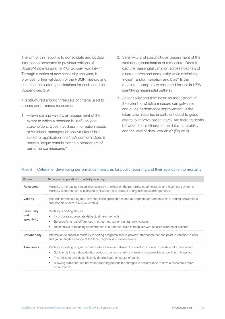
2. Sensitivity and specificity: an assessment of the statistical discrimination of a measure. Does it capture meaningful variation across hospitals of different sizes and complexity while minimising ‘noise’, random variation and bias? Is the measure appropriately calibrated for use in NSW, identifying meaningful outliers?
3. Actionability and timeliness: an assessment of the extent to which a measure can galvanise and guide performance improvement. Is the information reported in sufficient detail to guide efforts to improve patient care? Are there tradeoffs between the timeliness of the data, its reliability and the level of detail available? (Figure 5).
The aim of this report is to consolidate and update information presented in previous editions of Spotlight on Measurement for 30-day mortality.2,5 Through a series of new sensitivity analyses, it provides further validation of the RSMR method and describes indicator specifications for each condition (Appendices 3-9).
It is structured around three sets of criteria used to assess performance measures:
1. Relevance and validity: an assessment of the extent to which a measure is useful to local stakeholders. Does it address information needs of clinicians, managers or policymakers? Is it suited for application in a NSW context? Does it make a unique contribution to a broader set of performance measures?
Figure 5 Criteria for developing performance measures for public reporting and their application to mortality
Criteria Details and application to mortality reporting
Relevance Mortality is increasingly used internationally to reflect on the performance of hospitals and healthcare systems. Mortality outcomes are sensitive to clinical care and a range of organisational arrangements.
Validity Methods for measuring mortality should be applicable to and appropriate for data collection, coding conventions, and models of care in a NSW context.
Sensitivity and specificity
Mortality reporting should:
• Incorporate appropriate risk-adjustment methods
• Be specific to real differences in outcomes, rather than random variation
• Be sensitive to meaningful differences in outcomes, even in hospitals with smaller volumes of patients.
Actionability Information released in mortality reporting programs should provide information that can point to variation in care and guide tangible change at the local, regional and system levels.
Timeliness Mortality reporting programs must strike a balance between the need to produce up-to-date information and:
• Sufficiently long data collection periods to ensure stability of results for a sizeable proportion of hospitals
• The ability to provide sufficiently detailed data on cause of death
• Allowing sufficient time between reporting periods for changes in performance to have a discernible effect on outcomes.

13 Spotlight on Measurement: Measuring 30-day mortality following hospitalisation bhi.nsw.gov.au

14Spotlight on Measurement: Measuring 30-day mortality following hospitalisation bhi.nsw.gov.au
1. Relevance and validity
15 Spotlight on Measurement: Measuring 30-day mortality following hospitalisation bhi.nsw.gov.au
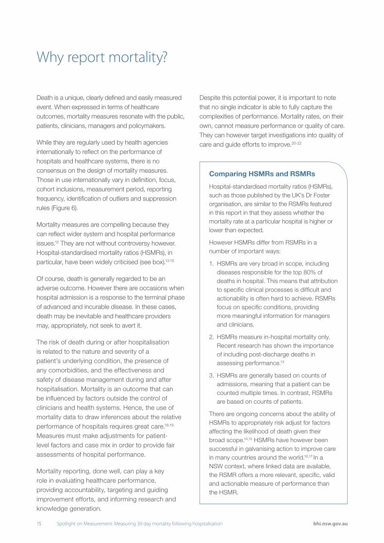
Death is a unique, clearly defined and easily measured event. When expressed in terms of healthcare outcomes, mortality measures resonate with the public, patients, clinicians, managers and policymakers.
While they are regularly used by health agencies internationally to reflect on the performance of hospitals and healthcare systems, there is no consensus on the design of mortality measures. Those in use internationally vary in definition, focus, cohort inclusions, measurement period, reporting frequency, identification of outliers and suppression rules (Figure 6).
Mortality measures are compelling because they can reflect wider system and hospital performance issues.12 They are not without controversy however. Hospital-standardised mortality ratios (HSMRs), in particular, have been widely criticised (see box).13-15
Of course, death is generally regarded to be an adverse outcome. However there are occasions when hospital admission is a response to the terminal phase of advanced and incurable disease. In these cases, death may be inevitable and healthcare providers may, appropriately, not seek to avert it.
The risk of death during or after hospitalisation is related to the nature and severity of a patient’s underlying condition, the presence of any comorbidities, and the effectiveness and safety of disease management during and after hospitalisation. Mortality is an outcome that can be influenced by factors outside the control of clinicians and health systems. Hence, the use of mortality data to draw inferences about the relative performance of hospitals requires great care.18,19 Measures must make adjustments for patient-level factors and case mix in order to provide fair assessments of hospital performance.
Mortality reporting, done well, can play a key role in evaluating healthcare performance, providing accountability, targeting and guiding improvement efforts, and informing research and knowledge generation.
Despite this potential power, it is important to note that no single indicator is able to fully capture the complexities of performance. Mortality rates, on their own, cannot measure performance or quality of care. They can however target investigations into quality of care and guide efforts to improve.20-22
Why report mortality?
Comparing HSMRs and RSMRs
Hospital-standardised mortality ratios (HSMRs), such as those published by the UK’s Dr Foster organisation, are similar to the RSMRs featured in this report in that they assess whether the mortality rate at a particular hospital is higher or lower than expected.
However HSMRs differ from RSMRs in a number of important ways:
1. HSMRs are very broad in scope, including diseases responsible for the top 80% of deaths in hospital. This means that attribution to specific clinical processes is difficult and actionability is often hard to achieve. RSMRs focus on specific conditions, providing more meaningful information for managers and clinicians.
2. HSMRs measure in-hospital mortality only. Recent research has shown the importance of including post-discharge deaths in assessing performance.13
3. HSMRs are generally based on counts of admissions, meaning that a patient can be counted multiple times. In contrast, RSMRs are based on counts of patients.
There are ongoing concerns about the ability of HSMRs to appropriately risk adjust for factors affecting the likelihood of death given their broad scope.14,15 HSMRs have however been successful in galvanising action to improve care in many countries around the world.16,17 In a NSW context, where linked data are available, the RSMR offers a more relevant, specific, valid and actionable measure of performance than the HSMR.

16Spotlight on Measurement: Measuring 30-day mortality following hospitalisation bhi.nsw.gov.au
Figure 6 Hospital mortality measures in other countries
USA Centers for Medicare & Medicaid Services6
Canadian Institute for Health Information7
England Health & Social Care Information Centre8
England Dr Foster Intelligence9
Scotland Information Services Division10
Statistics
Netherlands11
Measure
Risk-standardised Mortality Rate (RSMR)
Hospital-standardised Mortality Ratio (HSMR)
Summary Hospital-level Mortality Indicator (SHMI)
Hospital-standardised Mortality Ratio (HSMR)
Hospital-standardised Mortality Ratio (HSMR)
Hospital-standardised Mortality Ratio (HSMR), diagnosis-specific Standardised Mortality Ratio (SMR)
Definition
Deaths within 30 days of admission
Deaths in hospital Deaths in hospital or within 30 days of discharge
Deaths in hospital Deaths within 30 days of admission
Deaths in hospital
Focus diagnoses
Acute myocardial infarction (AMI)
Heart failure
Pneumonia
Chronic obstructive pulmonary disease
Ischaemic stroke
Diagnosis groups that account for about 80% of in hospital deaths
All conditions Diagnosis groups that account for about 80% of in hospital deaths
All conditions Diagnosis groups that account for about 80% of in hospital deaths
Cohort inclusions
Age 65+ years enrolled in Medicare. Veterans Affairs beneficiaries also included for AMI, heart failure and pneumonia.
Age 29 days – 120 years
Age 0–120 years Age 0–120 years All ages All ages
Measurement period
One year and rolling three years
Quarter year and year to date
Rolling 12 months One year and rolling three years
Quarter year and rolling 12 months
One year and rolling three years
Reporting frequency
Annually Quarterly Quarterly Annually Quarterly Annually
Results
RSMR with 95% interval estimate
HSMR with 95% confidence interval
Funnel plot with 95% control limits
HSMR with 95% confidence interval, funnel plot with 99.8% control limits
Trend HSMR with regression line
HSMR and SMR with 95% confidence interval, funnel plot with 95% and 99.8% control limits
Suppression rule
Suppress results for hospitals with fewer than 25 cases
Suppress results for hospitals with fewer than 20 expected deaths
HSMRs and SMRs not calculated for hospitals with fewer than 60 observed deaths in all inpatient admissions

17 Spotlight on Measurement: Measuring 30-day mortality following hospitalisation bhi.nsw.gov.au
Analyses in BHI reports on 30-day mortality included patients admitted to both public and private hospitals. RSMRs were published for public hospitals only as BHI does not have the authority to report private hospital performance.
Collectively, private hospitals had lower than expected mortality for five conditions analysed for the 2009–12 period. This may be a reflection of lower mortality at private hospitals. Alternatively, it may be that the patients at private hospitals were systematically different from patients at public hospitals and the adjustments made by BHI to account for case mix were unable to capture all of these differences.
In producing RSMRs for each condition, BHI adjusts for age, sex and relevant comorbidities. Including private hospital patients had a small impact on the coefficients of the predictive models, producing a dampening effect on each public hospital’s expected number of deaths. If the differences in mortality between public and private hospital patients are a reflection of different risk profiles that the modelling is unable to take account of, including private hospital patients in the analyses may unfairly affect the results of public hospitals.
To ensure that fair assessments are made, one option is to exclude private hospital patients from analyses. Sensitivity analyses were conducted to investigate the impact of excluding private hospital patients from the 2009–12 cohorts for five conditions.
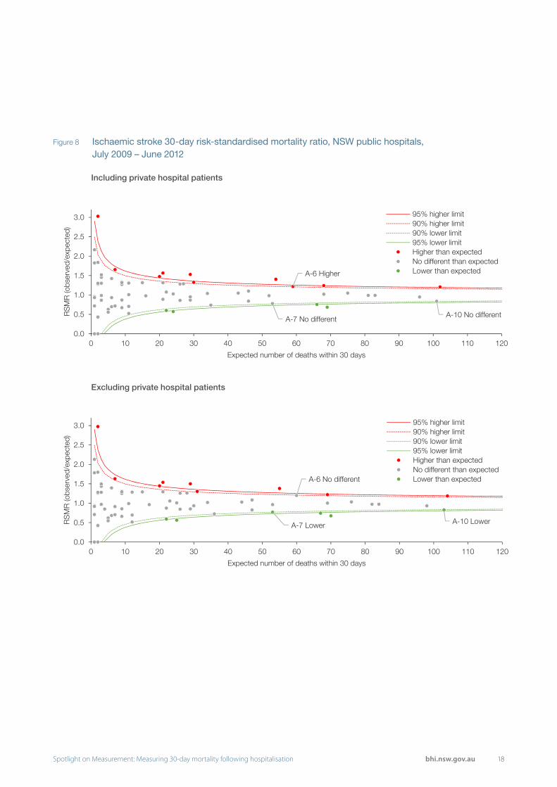
Excluding private hospital patients was not expected to change the RSMRs substantially as they comprised only a small proportion of the cohort for each condition (Figure 7). However, even a small change in RSMRs could alter the status of hospitals close to the control limits.
For the five conditions, the variables in the risk adjustment model did not change and the model C-statistics decreased by less than 0.01. Among hospitals with at least one expected death, the RSMRs either did not change (for those hospitals with no observed deaths) or decreased slightly. Across all conditions the maximum decrease in RSMR was 0.05.
There was a change in outlier hospitals for ischaemic stroke and pneumonia. For ischaemic stroke, one hospital was no longer higher than expected and two hospitals became lower than expected (Figure 8). For pneumonia, one hospital became lower than expected. The RSMRs for these hospitals did not change substantially — they were close to the control limits and a small change was sufficient to change their status.
Including or excluding private hospital patients
Figure 7 Distribution of patients admitted to public and private hospitals in NSW, July 2009 – July 2012
Public hospitals Private hospitals
Acute myocardial infarction 28,494 (98%) 729 (2%)
Ischaemic stroke 13,794 (97%) 411 (3%)
Haemorrhagic stroke 5,544 (98%) 137 (2%)
Pneumonia 42,499 (96%) 1,560 (4%)
Hip fracture surgery 14,751 (93%) 1,085 (7%)
18Spotlight on Measurement: Measuring 30-day mortality following hospitalisation bhi.nsw.gov.au
Figure 8 Ischaemic stroke 30-day risk-standardised mortality ratio, NSW public hospitals, July 2009 – June 2012
Including private hospital patients
Excluding private hospital patients
A-6 Higher
A-7 No different A-10 No different
0.0
0.5
1.0
1.5
2.0
2.5
3.0
0 10 20 30 40 50 60 70 80 90 100 110 120
RS
MR
(obs
erve
d/ex
pect
ed)
Expected number of deaths within 30 days
95% higher limit90% higher limit90% lower limit95% lower limitHigher than expectedNo different than expectedLower than expected
A-6 No different
A-7 Lower A-10 Lower
0.0
0.5
1.0
1.5
2.0
2.5
3.0
0 10 20 30 40 50 60 70 80 90 100 110 120
RS
MR
(obs
erve
d/ex
pect
ed)
Expected number of deaths within 30 days
95% higher limit90% higher limit90% lower limit95% lower limitHigher than expectedNo different than expectedLower than expected

19 Spotlight on Measurement: Measuring 30-day mortality following hospitalisation bhi.nsw.gov.au
Figure 10 Maximum decrease and increase in RSMRs if same-day discharge and admission treated as a transfer, July 2009 – June 2012*
Condition Maximum decrease Maximum increase
Acute myocardial infarction -0.222 +0.430
Ischaemic stroke -0.431 +0.027
Haemorrhagic stroke -0.120 +0.132
Pneumonia -0.052 +0.057
Hip fracture surgery -0.002 +0.015
Figure 9 Patients with same-day discharge and admission, July 2009 – June 2012
Hospital performance measures rely on the quality of the data on which they are based. Linked admitted patient and fact of death data are used by BHI to produce RSMRs. A series of data quality checks are applied to admitted patient data by the data custodian to reduce the risk of anomalies.23 The coding of principal diagnosis in NSW hospitals has been found to be accurate with positive predictive values consistently over 95%.24-26 The admitted patient and fact of death data are probabilistically linked by the Centre for Health Record Linkage (CHeReL). The linked data has a false positive rate (incorrect link) and a false negative rate (missed link) of about 5/1000.27
Despite quality checks, inconsistencies in coding occur and this can affect hospitals’ results for measures that are based on administrative datasets. One variable in the admitted patient data that may contain anomalies is the mode of separation.
Some patients may be incorrectly coded as discharged from hospital when they were in fact transferred to another hospital. This will affect the accuracy of the RSMRs.
In BHI reports on 30-day mortality, patients who were transferred between different hospitals during their period of care were attributed to the first hospital to which they were admitted. The reason for this is that the first few hours and days of treatment are crucial to survival, particularly for AMI and stroke. If a patient was transferred but this event was recorded as a discharge, the patient will be incorrectly attributed to the second hospital within a new period of care, and the first hospital will not be included in the analysis.
Coding of transfers between hospitals
* RSMRs for hospitals with an expected mortality ≥ 1.0.
Condition Same-day patients Total patients %
Acute myocardial infarction 176 29,223 0.60
Ischaemic stroke 53 14,205 0.37
Haemorrhagic stroke 23 5,681 0.40
Pneumonia 163 44,059 0.37
Hip fracture surgery <5 15,836 <0.05

20Spotlight on Measurement: Measuring 30-day mortality following hospitalisation bhi.nsw.gov.au
Figure 11 Pneumonia 30-day risk-standardised mortality ratio, NSW public hospitals, July 2009 – June 2012
Same-day discharge and admission not treated as a transfer
Same-day discharge and admission treated as a transfer
A-12 No different
0.0
0.5
1.0
1.5
2.0
2.5
3.0
0 20 40 60 80 100 120 140 160 180 200 220
RS
MR
(obs
erve
d/ex
pect
ed)
Expected number of deaths within 30 days
95% higher limit90% higher limit90% lower limit95% lower limitHigher than expectedNo different than expectedLower than expected
A-12 Lower
0.0
0.5
1.0
1.5
2.0
2.5
3.0
0 20 40 60 80 100 120 140 160 180 200 220
RS
MR
(obs
erve
d/ex
pect
ed)
Expected number of deaths within 30 days
95% higher limit90% higher limit90% lower limit95% lower limitHigher than expectedNo different than expectedLower than expected
The impact of a potential miscode in the mode of separation was investigated. During the period July 2009 – June 2012 across five conditions, between 0.05% and 0.60% of the cohorts had a same-day discharge and admission (Figure 9).
Periods of care were reconstructed assuming that patients with same-day discharge and admission had been miscoded and were actually transferred. RSMRs were reproduced and results compared. The condition most affected was AMI, for which the change in RSMRs ranged from a decrease of 0.222 to an increase of 0.430 (Figure 10).
Outliers were identified for each condition based on the new RSMRs. One hospital became a low mortality outlier for pneumonia (Figure 11). Its RSMR decreased by 0.004 and this was sufficient to change its status. There were no changes to outliers for the other conditions.
Given that there are some inconsistencies in coding, the analyses for the final report considered same-day discharges and admission as transfers, attributing outcomes to the first hospital.

21 Spotlight on Measurement: Measuring 30-day mortality following hospitalisation bhi.nsw.gov.au
Mortality is an important outcome measure — one that gauges the impact or results of healthcare. Outcomes are influenced by issues such as patient risk factors, models of care, and access to different providers of care — meaning that responsibility for performance can be difficult to attribute. Statistical methods such as the RSMR take account of a range of patient-level factors that impact mortality in order to make fair assessments of hospital performance in an effort to ensure that any significant variation measured reflects actual differences in care.
One way to assess whether risk-adjusted outcome measures reflect performance is to compare them with process measures. Process measures focus on the care that was delivered to patients and whether it was in accordance with the evidence base or models of best practice. While 100% concordance is never achieved, establishing an association between outcomes (30-day mortality) and process measures (delivery of evidence-based, high quality care) can support two conclusions. First, it provides validation that the outcome measure is reflecting variation in the quality of care delivered. Second, it means that outlier status can act as a signal to examine those specific processes of care for opportunities to improve.
The Agency for Clinical Innovation (ACI) and its predecessor organisation, the Greater Metropolitan Clinical Taskforce, have since 2002 been engaged in building and strengthening a clinical network for stroke across NSW, seeking to improve processes of care. A key part of the network’s activities is the development and application of audit tools to guide quality improvement across the state’s public hospitals.
ACI audit tools are evidence-based, and include clinical performance indicators advocated by the National Stroke Foundation.28 A range of stroke care processes are measured, including the proportion of patients admitted to a dedicated stroke unit, the use of timely brain imaging, the provision of appropriate allied health assessments, the recording of neurological observations, and the use of clinical pathways.29
Figure 12 examines patterns of overall performance from ACI stroke audits, placing them alongside RSMR results for the period July 2009 – June 2012. The results show some concordance between a hospital’s RSMR result and the process measures used in the audit. No hospital with a higher than expected RSMR had strongly favourable relative performance on process measures included in the stroke audit. Conversely, hospitals that performed well in the audit were more likely to record lower than expected RSMRs.
The results suggest that RSMRs have some validity as screening tools to assess performance in stroke care — able to identify where to look for exemplars of excellence as well as where efforts to improve should focus.
Associations between outcomes and processes

22Spotlight on Measurement: Measuring 30-day mortality following hospitalisation bhi.nsw.gov.au
Figure 12 Association between July 2009 – June 2012 RSMR for ischaemic stroke and relative performance in ACI stroke audit
Hos
pita
l 1
Hos
pita
l 2
Hos
pita
l 3
Hos
pita
l 4
Hos
pita
l 5
Hos
pita
l 6
Hos
pita
l 7
Hos
pita
l 8
Hos
pita
l 9
Hos
pita
l 10
Hos
pita
l 11
Hos
pita
l 12
Hos
pita
l 13
Hos
pita
l 14
RSMR • • • • • • • • • • • • • •% of patients admitted to a stroke unit/ICU or high-dependency unit
% of patients with neurological observations recorded in first 24 hours of hospitalisation
% of patients on stroke clinical pathway during admission
% of patients receiving swallow test within four hours of admission
% of patients discharged on an anti-thrombotic (if ischaemic stroke)
% of patients who received aspirin within 24 hours of admission (if ischaemic stroke)
% of patients discharged on a statin
% of patients on prophylaxis for deep vein thrombosis (if immobile)
• RSMR higher than expected
• RSMR no different than expected
• RSMR lower than expected
Favourable performance on audit measure

23 Spotlight on Measurement: Measuring 30-day mortality following hospitalisation bhi.nsw.gov.au
Ischaemic stroke severity and transient ischaemic attack
An ischaemic stroke occurs when a blood vessel is blocked, depriving the brain of oxygen and nutrients. As a result, the area of the brain supplied or drained by the blood vessel suffers damage. The severity and consequences of stroke can vary from complete recovery to severe disability or death.
Severity
Severity is an important predictor of mortality for ischaemic stroke.30 However there is mixed evidence about the impact of including severity in 30-day mortality models.31,32 Stroke RSMRs published in the United States by the Centers for Medicare and Medicaid Services (CMS) do not adjust for severity.6
Where available, the National Institutes of Health Stroke Scale provides a potential risk adjustment, however these data are not available in administrative databases in NSW. Other work in NSW has used Australian Refined Diagnosis Related Group codes as a proxy for disease severity in risk adjustment methods.33 However this coding can reflect outcomes (e.g. catastrophic complications, including death) as well as severity of disease on presentation, so is not suitable for use as a risk adjustment variable.
A transient ischaemic attack (TIA or ‘mini-stroke’) has the same underlying cause as a stroke – disruption of cerebral blood flow – and has similar symptoms, but they are temporary and resolve naturally within 24 hours. TIAs have far lower mortality than ischaemic stroke (12% for ischaemic stroke, 1% for TIA for the 2012–15 period) and so differences in the way hospitals diagnose and code TIAs and strokes could introduce a bias.
To explore this issue the ratio of principal diagnoses for ischaemic stroke to TIA by hospital for the period July 2012 to June 2015 was calculated (Figure 13).
As hospital size increases, in terms of the number of episodes with ischaemic stroke or TIA as the principal diagnosis, the ratio of ischaemic stroke to TIA increases. It may be that smaller hospitals receive fewer patients with more complicated conditions. Alternatively, there may be some level of misdiagnosing or miscoding an ischaemic stroke as a TIA. This error will result in valid patients being excluded from the ischaemic stroke cohort and may bias RSMRs.
RSMRs for patients aged 15 years or over who were discharged between 1 July 2012 and 30 June 2015 with an acute, emergency admission for a principal diagnosis of ischaemic stroke (ICD-10-AM code I63) or TIA (ICD-10-AM code G45) were calculated. The cohort increased from 15,475 patients with ischaemic stroke to 29,012 patients with ischaemic stroke or TIA. The same risk adjustment variables were used – age, sex, renal failure, heart failure, and malignancy – as well as a variable for ischaemic stroke or TIA.
When TIA was added to the ischaemic stroke cohort, there was a change in hospital outliers (Figure 14). Two hospitals became high (one would not be publicly reported) and two became low. Six hospitals remained high and one remained low.
The addition of TIA patients to the ischaemic stroke cohort did not result in a substantial change in RSMRs. There may be some misdiagnosis or miscoding of ischaemic stroke and TIA but it does not appear to be biasing ischaemic stroke RSMRs.
There is some evidence that a TIA may reduce the severity of a subsequent ischaemic stroke.34 For the ischaemic stroke cohort only, we tested the inclusion of a variable for a TIA diagnosis in the year prior to the index admission, but it was not significantly associated with 30-day mortality.

24Spotlight on Measurement: Measuring 30-day mortality following hospitalisation bhi.nsw.gov.au
Figure 13 Ratio of ischaemic stroke to transient ischaemic attack principal diagnoses, July 2012 – June 2015 (Peer group A-C hospitals with at least 50 episodes)
0.0
0.5
1.0
1.5
2.0
2.5
3.0
0 200 400 600 800 1,000 1,200 1,400 1,600
Rat
io is
chae
mic
str
oke
to
TIA
prin
cipa
l dia
gnos
es
Total episodes with ischaemic stroke or TIA as principal diagnosis
Figure 14 Ischaemic stroke and transient ischaemic attack 30-day risk-standardised mortality ratio, NSW public hospitals, July 2012 – June 2015
C2-31* No different
BNM-9 No different
A-2 No differentA-11 No different
0.0
0.5
1.0
1.5
2.0
2.5
3.0
3.5
4.0
0 20 40 60 80 100 120 140 160 180 200 220
RS
MR
(obs
erve
d/ex
pect
ed)
Expected number of deaths within 30 days
99.8% upper limit95% higher limit95% lower limit99.8% lower limitHigher than expectedNo different than expectedLower than expected
C2-31* Higher
BNM-9 Higher
A-2 Lower A-11 Lower
0.0
0.5
1.0
1.5
2.0
2.5
3.0
3.5
4.0
0 20 40 60 80 100 120 140 160 180 200 220
RS
MR
(obs
erve
d/ex
pect
ed)
Expected number of deaths within 30 days
99.8% upper limit95% higher limit95% lower limit99.8% lower limitHigher than expectedNo different than expectedLower than expected
Ischaemic stroke
Ischaemic stroke and transient ischaemic attack
* These hospitals would not be publicly reported.

25 Spotlight on Measurement: Measuring 30-day mortality following hospitalisation bhi.nsw.gov.au
Hip fracture surgery at first hospital
The cohort for hip fracture surgery comprises patients aged 50+ years hospitalised with a principal diagnosis of hip fracture, as well as a fall-related diagnosis and a hip fracture surgery procedure code. Surgery is indicated in all but very advanced palliative care patients – providing pain relief as well as restoring mobility. Patients who did not receive surgery are generally excluded from RSMR analyses.
During 2012–15, 87% of hip fracture patients aged 50+ years underwent surgery in NSW hospitals. A small proportion of NSW patients underwent surgery interstate but outcome data are not available for these patients.
While BHI does not have access to interstate hospital data, it does have access to the NSW Health Clinical Services Planning Analytics (CaSPA) Portal which includes information on patient flows. For the 2012–15 period, 19,510 patients residing in NSW had a hip fracture diagnosis and a hip fracture surgery procedure code according to data in CaSPA. Of these 19,510 patients, 514 (2.6%) were treated at an interstate hospital.
Differences across hospitals in the propensity to perform surgery on hip fracture patients could bias results with higher mortality among those hospitals with higher rates of surgery.
The percentage of patients with hip fracture from a fall that did not receive surgery at the first admitting hospital nor at another NSW hospital are presented by the first admitting hospital (Figure 15). There were some small hospitals not performing surgery nor transferring for surgery for a substantial proportion of patients but most hospitals had a similar rate. Note, the hospital with the highest rate (83%) has a model of care to transfer patients interstate for surgery.
For 30-day mortality following hip fracture surgery, the outcome is attributed to the hospital that performed the surgery. Hospitals that receive a lot of hip fracture patients for surgery from other hospitals may be disadvantaged by delays in transfer. Among peer group A-C hospitals with at least 50 patients, the percentage of hip fracture patients that were admitted to another hospital and transferred for surgery ranged from 0% to 56%. However, there was no clear relationship between this percentage and the low or high mortality hospitals (Figure 16).
Crude mortality rates stratified by whether or not patients were admitted to another hospital prior to transfer for surgery were compared. Overall, the crude mortality rate for patients that were first admitted to another hospital was 7.4% compared to 6.7% for patients that were not.
† Some patients may have received surgery interstate but BHI does not have access to interstate hospital data.
* This hospital has a model of care to transfer patients interstate for surgery.
0
10
20
30
40
50
60
70
80
90
100
0 200 400 600 800 1000 1200 1400
Did
not
rec
eive
sur
gery
(%)
Patients
*
Figure 15 Percent of hip fracture patients that did not receive surgery by first admitting hospital, July 2012 – June 2015 (Peer group A-C hospitals with at least 50 patients)†

26Spotlight on Measurement: Measuring 30-day mortality following hospitalisation bhi.nsw.gov.au
Hospital 1 55%Hospital 2 23%Hospital 3 56%Hospital 4 26%Hospital 5 49%Hospital 6 15%Hospital 7 48%Hospital 8 7%Hospital 9 8%Hospital 10 6%Hospital 11 9%Hospital 12 42%Hospital 13 28%Hospital 14 34%Hospital 15 12%Hospital 16 16%Hospital 17 7%
Transferred infor surgery %
*
*
0 1 2 3 4 5 6 7 8 9 10 11 12 13 14 15 16 17 18 19 20
Crude mortality rate (per 100)
Was not transferred in Was transferred in
Figure 17 Hip fracture surgery, crude mortality by whether patient transferred in for surgery, July 2012 – June 2015†
† Peer group A-C hospitals with at least 50 patients overall and at least five patients and 5% admitted to another hospital.
* Crude mortality significantly different based on Fisher’s exact test.
Among hospitals with at least five patients first admitted to another hospital (and they accounted for at least 5% of all of their patients), the difference between the crude mortality rate for its patients that were first admitted to another hospital and its patients that were not, ranged from -5 to +14 (Figure 17). Only two of these differences were statistically significant (based on Fisher’s exact test
at the 0.05 level of significance) but neither of these hospitals had high mortality. Among the high mortality outliers, the crude mortality rate for patients that first presented to another hospital were actually lower.
Therefore the issue of patients first admitted to another hospital does not seem to bias RSMRs.
Figure 16 Proportion of index case patients who were transferred in from another hospital for hip fracture surgery, July 2012 – June 2015 (Peer group A-C hospitals with at least 50 patients)
Hip fracture surgery
NSW (13%)
0 10 20 30 40 50 60 70 80 90 100
% of patients
Lower than expected mortality No different than expected mortality Higher than expected mortality
Lower than expected mortality No different than expected mortality Higher than expected mortality

27 Spotlight on Measurement: Measuring 30-day mortality following hospitalisation bhi.nsw.gov.au
Presentation to an emergency department prior to admission
In cases of transfer within an index hospitalisation, patients and their outcomes are attributed to the first admitting hospital. This approach is consistent with attribution conventions in other jurisdictions and is sensitive to the role played by smaller hospitals in stabilisation and prompt transfer of patients to larger specialist facilities.
For each of the seven conditions included in the RSMR analyses, the majority of patients were admitted to the first hospital through its emergency department (ED). However, there are cases where a patient first presented to a hospital’s ED but, instead of being admitted to that hospital, they were transferred to a different hospital and admitted. According to the established attribution rules, these patients are attributed to the admitting hospital, not the hospital where the patient presented to its ED.
This analysis explored the extent to which hospitals are affected by ‘pseudo-transfers’.
Among peer group A-C hospitals with at least 50 patients, the percentage of patients that visited another hospital’s ED in the 24 hours prior to the index admission varied across the AMI (0% to 34%), ischaemic stroke (0% to 39%) and hip fracture surgery cohorts (0% to 49%) (see Figure 18 for ischaemic stroke and Appendix 10 for AMI and hip fracture surgery).
There was no clear relationship between the percentage of patients who had visited another hospital ED prior to admission and outlier status. Among high mortality hospitals, some had a very low percentage of patients visiting another ED and some had a very high percentage.
The crude mortality rates for patients that did and did not visit another hospital’s ED in the 24 hours prior to the index hospitalisation were also compared. Overall, the crude mortality rate for patients that visited another ED was 0.2% higher for AMI, 1.3% lower for ischaemic stroke and 0.7% higher for hip fracture surgery, compared to those for patients that did not visit another ED.
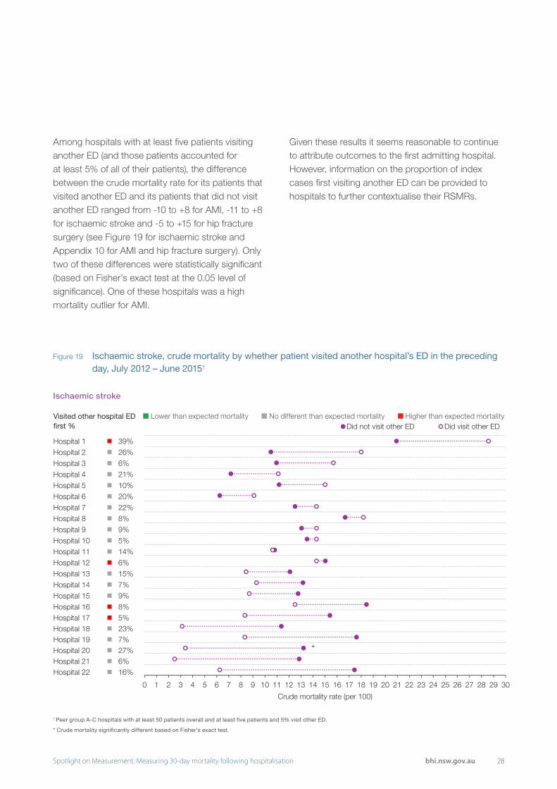
Figure 18 Proportion of ischaemic stroke patients who visited another hospital’s ED in the preceding day, July 2012 – June 2015 (Peer group A-C hospitals with at least 50 patients)
Ischaemic stroke
NSW (7%)
0 10 20 30 40 50 60 70 80 90 100
% of patients
Lower than expected mortality No different than expected mortality Higher than expected mortality
28Spotlight on Measurement: Measuring 30-day mortality following hospitalisation bhi.nsw.gov.au
Hospital 1 39%Hospital 2 26%Hospital 3 6%Hospital 4 21%Hospital 5 10%Hospital 6 20%Hospital 7 22%Hospital 8 8%Hospital 9 9%Hospital 10 5%Hospital 11 14%Hospital 12 6%Hospital 13 15%Hospital 14 7%Hospital 15 9%Hospital 16 8%Hospital 17 5%Hospital 18 23%Hospital 19 7%Hospital 20 27%Hospital 21 6%Hospital 22 16%
Visited other hospital ED first %
*
0 1 2 3 4 5 6 7 8 9 10 11 12 13 14 15 16 17 18 19 20 21 22 23 24 25 26 27 28 29 30
Crude mortality rate (per 100)
Did not visit other ED Did visit other ED
Figure 19 Ischaemic stroke, crude mortality by whether patient visited another hospital’s ED in the preceding day, July 2012 – June 2015†
Ischaemic stroke
† Peer group A-C hospitals with at least 50 patients overall and at least five patients and 5% visit other ED.
* Crude mortality significantly different based on Fisher’s exact test.
Lower than expected mortality No different than expected mortality Higher than expected mortality
Among hospitals with at least five patients visiting another ED (and those patients accounted for at least 5% of all of their patients), the difference between the crude mortality rate for its patients that visited another ED and its patients that did not visit another ED ranged from -10 to +8 for AMI, -11 to +8 for ischaemic stroke and -5 to +15 for hip fracture surgery (see Figure 19 for ischaemic stroke and Appendix 10 for AMI and hip fracture surgery). Only two of these differences were statistically significant (based on Fisher’s exact test at the 0.05 level of significance). One of these hospitals was a high mortality outlier for AMI.
Given these results it seems reasonable to continue to attribute outcomes to the first admitting hospital. However, information on the proportion of index cases first visiting another ED can be provided to hospitals to further contextualise their RSMRs.

29 Spotlight on Measurement: Measuring 30-day mortality following hospitalisation bhi.nsw.gov.au
Acute myocardial infarction
NSW (10%)
0 10 20 30 40 50 60 70 80 90 100
% of patients
Lower than expected mortality No different than expected mortality Higher than expected mortality
The RSMR method attributes patients and their outcomes to the first admitting hospital in cases where patients are transferred during their index hospitalisation. As discussed in the previous section (pages 27–28), some patients may first present to a hospital’s ED and then be transferred to a different hospital for admission, but these patients are still attributed to the first admitting hospital. A related question is whether some hospitals have a model of care that admits patients for a short period before transfer.
The extent to which hospitals are affected by first day transfers for AMI, ischaemic stroke and hip fracture surgery for the period July 2012 to June 2015 was explored.
Among peer group A-C hospitals with at least 50 patients, there was variation in the percentage of patients that were transferred on the first day of their index hospitalisation, AMI ranged from 0% to 70%, ischaemic stroke 0% to 36%, and hip fracture surgery 0% to 25% (see Figure 20 for AMI and Appendix 11 for ischaemic stroke and hip fracture surgery). However, there was no clear relationship between first day transfer rate and hospital outlier status.
Crude mortality rates for patients that were and were not transferred on the first day were also compared. Overall, the crude mortality rate for patients that were transferred on the first day was 3.6% lower for AMI, 1.2% lower for ischaemic stroke and 1.0% higher for hip fracture surgery, compared to those for patients not transferred on the first day.
Among hospitals with at least five patients transferred on the first day (and those patients accounted for at least 5% of all of their patients), the difference between the crude mortality rate for its patients that were transferred on the first day and its patients that were not ranged from -16 to +4 for AMI, -24 to -5 for ischaemic stroke and -10 to +16 for hip fracture surgery (see Figure 21 for AMI and Appendix 11 for ischaemic stroke and hip fracture surgery). Among high mortality hospitals, one difference was statistically significant for AMI (based on Fisher’s exact test at the 0.05 level of significance) but for this hospital the crude mortality rate for patients transferred on the first day was lower than the rate for patients not transferred on the first day.
The current method of patient attribution does not appear to bias RSMRs against hospitals with a higher rate of first day patient transfer and can continue to be used. Information on first day transfer rates can be provided to hospitals to further contextualise their RSMRs.
Transfer on the first day of admission
Figure 20 Proportion of acute myocardial infarction patients who were transferred on the first day, July 2012 – June 2015 (Peer group A-C hospitals with at least 50 patients)

30Spotlight on Measurement: Measuring 30-day mortality following hospitalisation bhi.nsw.gov.au
Hospital 1 29%Hospital 2 10%Hospital 3 12%Hospital 4 21%Hospital 5 6%Hospital 6 16%Hospital 7 16%Hospital 8 22%Hospital 9 36%Hospital 10 40%Hospital 11 19%Hospital 12 23%Hospital 13 6%Hospital 14 6%Hospital 15 42%Hospital 16 30%Hospital 17 26%Hospital 18 44%Hospital 19 6%Hospital 20 50%Hospital 21 34%Hospital 22 15%Hospital 23 61%Hospital 24 35%Hospital 25 28%Hospital 26 36%Hospital 27 15%Hospital 28 59%Hospital 29 42%Hospital 30 16%Hospital 31 17%Hospital 32 19%Hospital 33 9%Hospital 34 70%Hospital 35 11%Hospital 36 40%Hospital 37 23%Hospital 38 13%Hospital 39 44%
Transferred day 1 %
*
**
**
*
**
0 1 2 3 4 5 6 7 8 9 10 11 12 13 14 15 16 17 18 19 20
Crude mortality rate (per 100)
Not transferred day 1 Transferred day 1
Figure 21 Acute myocardial infarction, crude mortality by whether patient transferred on the first day, July 2012 – June 2015†
Acute myocardial infarction
† Peer group A-C hospitals with at least 50 patients overall and at least five patients and 5% transferred first day.
* Crude mortality significantly different based on Fisher’s exact test.
Lower than expected mortality No different than expected mortality Higher than expected mortality

31 Spotlight on Measurement: Measuring 30-day mortality following hospitalisation bhi.nsw.gov.au
Palliative care admissions
Very few patients were excluded from the cohorts as a result of palliative care codes. The proportion of acute patients with palliative care admission in the year prior to, or in the 30 days following, index admission was also low – less than 1% and less than 4% respectively for each cohort (Figure 22).
At a hospital level, the largest range for the percentage of patients with a palliative care admission in the year prior was for CHF (0.0% to 4.8%); and for palliative care admission following 30 days was ischaemic stroke (0.0% to 12.7%) (Figures 23, 24). For these two examples, the level of variation decreased as hospital size increased (Figure 25 for ischaemic stroke and Appendix 12 for CHF).
For ischaemic stroke, three of the high outlier hospitals had a relatively high proportion of patients with a palliative care admission in the 30 days following admission. However, when analyses were restricted to patients with no palliative care admission, crude mortality rates remained relatively high – suggesting that the original results were not biased [data not shown].
Figure 22 Palliative care analysis, five conditions, July 2012 – June 2015
For all of the conditions that BHI reports RSMRs, the cohort is restricted to patients with an acute admission. Patients with a palliative care admission are excluded on the basis that they have a very different likelihood of death in the 30 days following admission. However, there was some concern that among patients with an acute admission, some may have had a ‘do not resuscitate’ or advance care directive that was not reflected in the hospital administrative record. If such patients are included in the cohort and concentrated in a subset of hospitals, it can introduce a potential bias in RSMRs.
To investigate this issue, a series of descriptive analyses were performed for ischaemic stroke, CHF, pneumonia, COPD and hip fracture surgery for 2012–15.
The analyses were the number of:
• Patients excluded from the initial RSMR cohorts due to a palliative care type code
• Acute care patients who had a palliative care admission in the year prior to the index hospitalisation
• Acute care patients who had a palliative care admission in the 30 days following the index hospitalisation.
Condition Acute care patients Palliative care patients excluded
Acute patients with palliative admission
in the year prior
Acute patients with palliative admission in the
following 30 days
Ischaemic stroke 15,475 99 (0.6%) 27 (0.2%) 477 (3.1%)
CHF 27,484 332 (1.2%) 137 (0.5%) 634 (2.3%)
Pneumonia 47,133 274 (0.6%) 321 (0.7%) 941 (2.0%)
COPD 30,525 157 (0.5%) 196 (0.6%) 626 (2.1%)
Hip fracture surgery 16,193 2 (<0.1%) 59 (0.4%) 166 (1.0%)

32Spotlight on Measurement: Measuring 30-day mortality following hospitalisation bhi.nsw.gov.au
0
10
20
30
40
50
Ischaemic stroke CHF Pneumonia COPD Hip fracture surgery
Pal
liativ
e ad
mis
sion
yea
r pr
ior
(%)
Figure 23 Percent of acute patients with palliative admission in the year prior, hospital range and NSW (Peer group A-C hospitals with at least 50 patients), July 2012 – June 2015
Figure 24 Percent of acute patients with palliative admission in the following 30 days, hospital range and NSW (Peer group A-C hospitals with at least 50 patients), July 2012 – June 2015
Figure 25 Ischaemic stroke percent of acute patients with palliative admission in the following 30 days by hospital size (Peer group A-C hospitals with at least 50 patients), July 2012 – June 2015
0
2
4
6
8
10
12
14
16
18
20
0 100 200 300 400 500 600 700 800 900 1000
Pal
liativ
e ad
mis
sion
follo
win
g 30
day
s (%
)
Number of acute ischaemic stroke patients
No different than expected mortality Lower than expected mortality Higher than expected mortalityLower than expected mortality No different than expected mortality Higher than expected mortality
0
10
20
30
40
50
Ischaemic stroke CHF Pneumonia COPD Hip fracture surgery
Pal
liativ
e ad
mis
sion
follo
win
g 30
day
s (%
)
NSWHospital range
NSWHospital range

33 Spotlight on Measurement: Measuring 30-day mortality following hospitalisation bhi.nsw.gov.au

34Spotlight on Measurement: Measuring 30-day mortality following hospitalisation bhi.nsw.gov.au
2. Sensitivity and specificity

35 Spotlight on Measurement: Measuring 30-day mortality following hospitalisation bhi.nsw.gov.au
The length of the measurement period used to produce RSMRs affects the number of hospitals reaching the reporting threshold of 50 patients.
While the modelling approach that underpins the RSMR is applicable to hospitals with a low volume of patients, results for hospitals with very few patients can be disproportionately affected by a small number of deaths. Because of this variability, it is common practice to suppress mortality indicator results for small hospitals. Suppression criteria vary across jurisdictions and agencies. For example, the USA Centers for Medicare & Medicaid Services does not publicly report RSMRs based on fewer than 25 cases;6 while the Canadian Institute for Health Information does not publicly report HSMRs based on fewer than 20 expected deaths.7
The BHI reports on 30-day mortality include results for NSW public hospitals from peer groups A–C*. However, RSMRs based on fewer than one expected death were excluded from the analysis and RSMRs based on fewer than 50 patients were not publicly reported. This is a conservative approach that sought to avoid unfair judgement of small hospitals where random variation can have a more substantial impact on the value of the RSMR.
For all peer group A–C hospitals to reach the nominal reporting threshold (50 patients), the measurement period would have to be increased beyond three years. However, adopting such a long measurement period has consequences for the interpretation and actionability of results. The RSMRs may be perceived as out-of-date and no longer reflective of current practice, consequently affecting motivation to investigate or change practice in response to the data.
Using a measurement period that is shorter than three years results in a smaller number of hospitals reaching the reporting threshold but the measure is more up-to-date. There is a trade-off between maximising the number of hospitals that can be reported on and providing the most current data that reflects performance.
The analysis summarised in Figure 26 explores the impact of using one-, two- or three-year measurement periods on the number of peer group A–C hospitals reaching the inclusion threshold and the nominal reporting threshold across five conditions.
Using a three-year measurement period rather than a one-year period increased the number of hospitals reaching the nominal reporting threshold by between 13% (for hip fracture surgery) and 167% (for haemorrhagic stroke). Corresponding increases in the number of reportable hospital results were 40% for acute myocardial infarction, 41% for ischaemic stroke and 17% for pneumonia.
Implications of one-, two-, or three-year measurement periods
* For a description of hospital peer groups, see Appendix 1

36Spotlight on Measurement: Measuring 30-day mortality following hospitalisation bhi.nsw.gov.au
Figure 26 Number of peer group A–C hospitals provided with an RSMR and reaching the nominal reporting threshold with one-, two- and three-year measurement periods, July 2009 – June 2012
Hospitals (at least one patient with
condition of interest)
Hospitals provided with an RSMR
(at least one expected death)
Hospitals reaching nominal
reporting threshold (at least 50 patients)
Acute myocardial infarction
One year 2011–12 81 63 47
40% increase
Two years 2010–12 81 76 56
Three years 2009–12 82 77 66
Ischaemic stroke
One year 2011–12 78 53 34
41% increase
Two years 2010–12 79 64 39
Three years 2009–12 82 71 48
Haemorrhagic stroke
One year 2011–12 75 59 12
167% increase
Two years 2010–12 78 70 25
Three years 2009–12 80 75 32
Pneumonia
One year 2011–12 82 78 66
17% increase
Two years 2010–12 83 79 75
Three years 2009–12 83 80 77
Hip fracture surgery
One year 2011–12 41 37 32
13% increase
Two years 2010–12 43 38 35
Three years 2009–12 44 38 36

37 Spotlight on Measurement: Measuring 30-day mortality following hospitalisation bhi.nsw.gov.au
The 2013 BHI report on 30-day mortality used funnel plots with 90% and 95% control limits to determine whether hospital RSMRs were significantly different from expected. The 2017 report uses more stringent 95% and 99.8% control limits.
Funnel plots are increasingly used to evaluate hospital performance. Widely considered to provide a fair way to interpret metrics such as RSMRs, funnel plots provide a way to take account of the greater random variability that can affect results in low-volume hospitals.35 Smaller hospitals appear to the left of the funnel plot where control limits are wider.
The length of the measurement period used to produce RSMRs affects patient volumes and the confidence that RSMRs are significantly high or low. As the number of years in the measurement period increases, patient volumes and the number of expected deaths increase. These increases mean that within the funnel plot, hospital results shift to the right where estimates are more precise and smaller deviations from the NSW average can be deemed statistically significant.
The impact of different time periods on the funnel plots was investigated with the ischaemic stroke cohort (Figure 27).
Funnel plots were produced for one-, two- and three-year periods (Figure 28). For individual hospitals, as the time period was increased from one to three years, the number of expected deaths (a reflection of patient volumes) increased up to threefold — with resulting shifts to the right within the funnel.
The number of hospitals with significantly higher or lower than expected mortality for ischaemic stroke was compared for discrete one-, two- and three-year periods from July 2000 – June 2012. Hospitals that had at least one expected death every year were included in the analysis. There were 48 hospitals, representing a total of 576 hospital years. The number of hospitals that were high or low in at least one period was greatest for the one-year analysis (28 high and 19 low). However for many hospitals, the outlier status was fleeting — limited to a single time period (Figure 27).
The number of hospital years with high or low mortality was highest for the three-year analysis (84 high and 42 low). Three-year periods capture more systematic variation in mortality outcomes, while one-year periods appear more susceptible to short-term, possibly random, variation.
The effect of different measurement periods
Figure 27 Ischaemic stroke, higher or lower than expected mortality for discrete one-, two- and three-year periods, July 2000 – June 2012 (48 hospitals with at least one expected death each year)
Discrete one year
Discrete two years
Discrete three years
Number of hospitals with:
Higher than expected mortality in at least one period
28 18 16
Lower than expected mortality in at least one period
19 10 8
Number of hospital years with:
Higher than expected mortality 55 64 84
Lower than expected mortality 29 34 42
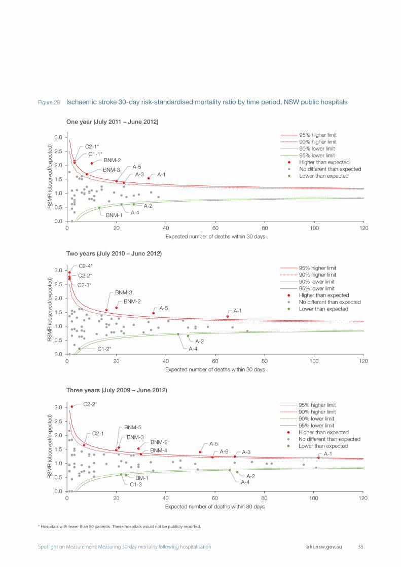
38Spotlight on Measurement: Measuring 30-day mortality following hospitalisation bhi.nsw.gov.au
Figure 28 Ischaemic stroke 30-day risk-standardised mortality ratio by time period, NSW public hospitals
* Hospitals with fewer than 50 patients. These hospitals would not be publicly reported.
One year (July 2011 – June 2012)
C2-1*C1-1*
BNM-3
BNM-2A-5A-3 A-1
BNM-1 A-4A-2
0.0
0.5
1.0
1.5
2.0
2.5
3.0
0 20 40 60 80 100 120
RS
MR
(obs
erve
d/ex
pect
ed)
Expected number of deaths within 30 days
95% higher limit90% higher limit90% lower limit95% lower limitHigher than expectedNo different than expectedLower than expected
C2-4*
C2-3*
C2-2*
BNM-3
BNM-2A-5 A-1
C1-2* A-4A-2
0.0
0.5
1.0
1.5
2.0
2.5
3.0
0 20 40 60 80 100 120
RS
MR
(obs
erve
d/ex
pect
ed)
Expected number of deaths within 30 days
95% higher limit90% higher limit90% lower limit95% lower limitHigher than expectedNo different than expectedLower than expected
C2-2*
C2-1BNM-5
BNM-3BNM-2
BNM-4A-5
A-6 A-3 A-1
C1-3BM-1
A-4A-2
0.0
0.5
1.0
1.5
2.0
2.5
3.0
0 20 40 60 80 100 120
RS
MR
(obs
erve
d/ex
pect
ed)
Expected number of deaths within 30 days
95% higher limit90% higher limit90% lower limit95% lower limitHigher than expectedNo different than expectedLower than expected
Two years (July 2010 – June 2012)
Three years (July 2009 – June 2012)

39 Spotlight on Measurement: Measuring 30-day mortality following hospitalisation bhi.nsw.gov.au
The control limits used in funnel plots to detect outlier hospitals affect the sensitivity and specificity of the measure. The higher the control limit is set, the lower the risk of false positives (flagging a hospital that is not truly different than expected) but the higher the risk of false negatives (failure to flag a hospital that is truly different than expected).
In most cases, control limits are set at 95% and/or 99.8%.8,9,11 At these levels, there is a small chance (one in 20 and two in 1,000, respectively) that an ‘in-control’ hospital would fall outside control limits.
In the development of the 2013 BHI report on 30-day mortality, 99.8% control limits identified few outliers. As the RSMR is designed to be used as a form of screening tool, sensitivity is important. Therefore 90% and 95% control limits were used to reduce the risk of false negatives while not substantially increasing the risk of false positives.
In general, 90% and 95% control limits flagged a greater proportion of large hospitals (peer groups A, BM and BNM) than small hospitals (peer groups C1 and C2).
This may be a reflection of a true difference in performance between small and large hospitals, or a consequence of insufficient precision in RSMRs for small hospitals to allow detection of outliers at 90% and 95% control limits.
To investigate this issue a sensitivity analysis was conducted on the control limits. The number of outliers among small and large hospitals was calculated for 95%, 90% and 80% control limits (Figure 29).
In practice, control limits would not be set at 80% for public reporting because it would greatly compromise specificity and increase the risk of false positives. However, if the proportion of outliers among small hospitals becomes similar to or greater than the proportion among large hospitals, it suggests that additional methods are needed to evaluate performance at small hospitals.
As control limits were lowered, there was a marked increase in the proportion of small hospitals with higher than expected mortality for ischaemic stroke, haemorrhagic stroke and pneumonia (Figure 29).
The effect of lowering control limits on the proportion of hospitals with lower than expected mortality was most discernible among large hospitals, particularly for ischaemic stroke and pneumonia. There was minimal change in the proportion of small hospitals that were low outliers (Figure 29).
Reducing the control limit did result in an increase in the proportion of high outliers among small hospitals relative to large hospitals for some conditions. This suggests that further analysis, in addition to funnel plots with 90% and 95% control limits, may be required to assess performance in small hospitals.
Varying funnel plot control limits

40Spotlight on Measurement: Measuring 30-day mortality following hospitalisation bhi.nsw.gov.au
Figure 29 Higher or lower than expected mortality at 80%, 90% and 95% control limits, by small hospitals (peer groups C1 and C2) and large hospitals (peer groups A, BM and BNM), July 2009 – June 2012
0% 10% 20% 30% 40% 50% 60% 70% 80% 90% 100%
95%90%80%95%90%80%
Large hospitals
Small hospitals
Con
trol
lim
it
n = 36
n = 41
Higher than expectedLower than expected No different than expected
0% 10% 20% 30% 40% 50% 60% 70% 80% 90% 100%
95%90%80%95%90%80%
Large hospitals
Small hospitals
Con
trol
lim
it
n = 36
n = 35
0% 10% 20% 30% 40% 50% 60% 70% 80% 90% 100%
95%90%80%95%90%80%
Large hospitals
Small hospitals
Con
trol
lim
it
n = 35
n = 40
0% 10% 20% 30% 40% 50% 60% 70% 80% 90% 100%
95%90%80%95%90%80%
Large hospitals
Small hospitals
Con
trol
lim
it
n = 36
n = 44
0% 10% 20% 30% 40% 50% 60% 70% 80% 90% 100%
95%90%80%95%90%80%
Large hospitals
Small hospitals
Con
trol
lim
it
n = 31
n = 7
* For hip fracture surgery, there are only seven small hospitals with patients compared to 31 large hospitals. The percentage of outliers for small and large hospitals for hip fracture surgery should be interpreted with caution.
Acute myocardial infarction
Ischaemic stroke
Haemorrhagic stroke
Pneumonia
Hip fracture surgery*

41 Spotlight on Measurement: Measuring 30-day mortality following hospitalisation bhi.nsw.gov.au
RSMRs are more variable for smaller hospitals (peer groups C1 and C2) than large hospitals (peer groups A, BM and BNM). Using haemorrhagic stroke to illustrate, the average standard deviation in three-year discrete RSMRs was 0.37 for small hospitals and 0.13 for large hospitals (Figure 30).
Low patient volumes at small hospitals mean that small, possibly random, changes in observed or expected deaths can have a substantial impact on RSMRs. Funnel plots make allowances for random variation that can affect the interpretation of results for small hospitals, making it possible to make fair assessments in any three-year time period.
There are concerns that some small hospitals may consistently record high mortality ratios but a low volume of patients in any one period means there is insufficient precision to identify them as outliers. This could be addressed by the use of a longer time period, but with consequences for the timeliness and actionability of results. One option is to flag a hospital that consistently records RSMRs over a pre-defined threshold, even if it fails to reach statistical significance.
This option was explored using discrete three-year haemorrhagic stroke RSMRs for small hospitals for July 2000 – June 2012 (Figure 31). Haemorrhagic stroke was used because of the substantial increase in small hospital outliers at 80% control limits.
Setting the RSMR threshold at 2.0 identified a single hospital, C2-14. In the original analysis, this hospital’s result reached statistical significance but the public reporting criterion of at least 50 patients was not met. Lowering the screening threshold, there were 20 RSMR results higher than 1.5, none of which reached statistical significance. No hospital had RSMRs greater than 1.5 for all four time periods. There were however six hospitals with RSMRs that were above 1.5 and not significant in multiple periods. For another eight hospitals, RSMRs fluctuated between above and below average, or they had too few patients in the other time periods to calculate an RSMR.
There are some concerns that small hospitals have reduced capacity to diagnose some conditions and may be diasadvantaged in comorbidity risk adjustment. Previous work has shown that there is only a modest trend towards fewer secondary diagnosis codes in smaller hospitals.2
Assessing mortality in small hospitals
Figure 30 Haemorrhagic stroke standard deviation in discrete three-year RSMRs, by small hospitals (peer groups C1 and C2) and large hospitals (peer groups A, BM and BNM), July 2000 – June 2012
0
10
20
30
40
0 0.2 0.4 0.6 0.8 1
Hos
pita
ls
RSMR standard deviation
0
10
20
30
40
0 0.2 0.4 0.6 0.8 1
Hos
pita
ls
RSMR standard deviation
Notes: Hospitals with at least one expected death in every period
Another option for small hospitals is the use of a Bayesian approach, where known information about other hospitals is used to produce estimates for small hospitals.36 Bayesian analyses were beyond the scope of this report but could be explored in the future
Small hospitals Large hospitals

42Spotlight on Measurement: Measuring 30-day mortality following hospitalisation bhi.nsw.gov.au
Figure 31 Haemorrhagic stroke discrete three-year RSMRs, small hospitals (peer groups C1 and C2), July 2000 – June 2012
Notes: Data for hospitals with an expected mortality < 1.0 are suppressed.
Hospitals with RSMR equal to zero had at least one expected death but no observed deaths.
For Hospital C2-14, the RSMR greater than 2 is statistically significant but would not be publicly reported.
0.0 1.0 2.0 3.0
C1-1C1-2C1-3C1-4C1-5C1-6C1-7C1-8C1-9
C1-10C1-11C1-12C1-13C1-14C2-1C2-2C2-3C2-4C2-5C2-6C2-7C2-8C2-9
C2-10C2-11C2-12C2-13C2-14C2-15C2-16C2-17C2-18C2-19C2-20C2-21C2-22C2-23C2-24C2-25C2-26C2-27C2-28C2-29C2-30C2-31
RSMRs in four time periods
Hos
pita
ls
NS
W
Higher than expected
Lower than expected
No different than expected (but with RSMR > 1.5)
No different than expected

43 Spotlight on Measurement: Measuring 30-day mortality following hospitalisation bhi.nsw.gov.au
Acute myocardial infarction (AMI) occurs when the heart muscle is damaged by lack of oxygen. BHI includes patients with a principal diagnosis of ICD-10-AM code I21 (acute myocardial infarction) in the AMI cohort. It does not include patients with a principal diagnosis of I22 (subsequent myocardial infarction). For the 2012–15 cohort, including this diagnosis would increase the number of patients by only 0.1%. The small number of patients with this diagnosis means that we may not adequately risk adjust for this subgroup and, even if we did, their inclusion would not have a material impact on results.
Within the I21 group, the AMI can be classified as ST-elevated myocardial infarction (STEMI) or non-ST-elevated myocardial infarction (non-STEMI) based on the electrocardiogram reading, or unspecified AMI when diagnostic records are unavailable.
STEMI status is an important predictor of mortality for AMI patients. STEMIs are associated with higher mortality at 30 days compared to non-STEMI (odds ratio = 1.55, 95% confidence interval 1.16-2.06).37 This means that a hospital with a relatively high proportion of STEMI patients could be expected to have higher mortality.
Across peer group A-C hospitals, the proportion of AMIs categorised as STEMI ranged between 4% and 53% for the 2012–15 period. This variation in STEMI rates suggests that risk adjustment should include STEMI status, assuming it is diagnosed and recorded similarly across hospitals.
The question regarding risk adjustment on the basis of STEMI-status is made more complex when the ‘STEMI non-specified’ group is considered.
Unspecified AMIs made up only 4% of AMI related admissions for the 2012–15 period, but 25% of 30-day mortality. The 30-day mortality for unspecified AMI was 51%, compared to 10% for STEMI and 5% for non-STEMI. Most of the mortality among unspecified AMI patients occurred on the day of
admission (58%), suggesting that one reason for this diagnosis was death of critically unwell patients before an electrocardiograph was done. However after excluding day-of-admission deaths, mortality for unspecified AMI patients was still higher than STEMI patients (31% compared to 8%).
The composition of the unspecified AMI group has changed over time. The number of unspecified AMIs has decreased but the rate of 30-day mortality has increased (Figure 32).
The proportion of AMI patients with unspecified AMI varies among hospitals. Hospitals with lower AMI patient volumes tend to have higher proportions of unspecified AMI. These hospitals remain higher even after excluding unspecified AMI patients that died on the day of admission. However the difference in proportion of unspecified AMI between small and large hospitals has decreased over time (Figure 33).
These findings suggest that the unspecified group is a heterogeneous mix of critically unwell patients who died before their AMI could be specified, and patients for whom diagnostic records were less precise. Including the unspecified group in a model that adjusts for STEMI status may have a spurious effect on calculations of expected mortality.
The impact of including the unspecified AMI group in the analysis, with and without adjusting for STEMI status is investigated on pages 45-46.
Describing acute myocardial infarction
Figure 32 Unspecified AMI patients over time, by 30-day outcome (death or survival)
01000200030004000500060007000
July 2003 –June 2006
July 2006 –June 2009
July 2009 –June 2012
July 2012 –June 2015
Pat
ient
s
Period
30-day deaths 30-day survivals

44Spotlight on Measurement: Measuring 30-day mortality following hospitalisation bhi.nsw.gov.au
July 2006 – June 2009
July 2009 – June 2012
July 2012 – June 2015
0
10
20
30
40
50
0 500 1000 1500 2000U
nspe
cifie
d A
MI (
%)
(exc
ludi
ng u
nspe
cifie
d A
MI
died
on
day
of a
dmis
sion
)
0
10
20
30
40
50
0 500 1000 1500 2000
Uns
peci
fied
AM
I (%
)
0
10
20
30
40
50
0 500 1000 1500 2000
Uns
peci
fied
AM
I (%
)(e
xclu
ding
uns
peci
fied
AM
Idi
ed o
n da
y of
adm
issi
on)
0
10
20
30
40
50
0 500 1000 1500 2000
Uns
peci
fied
AM
I (%
)
0
10
20
30
40
50
0 500 1000 1500 2000
Uns
peci
fied
AM
I (%
)(e
xclu
ding
uns
peci
fied
AM
Idi
ed o
n da
y of
adm
issi
on)
Number of AMI patients hospitalised
0
10
20
30
40
50
0 500 1000 1500 2000
Uns
peci
fied
AM
I (%
)
Number of AMI patients hospitalised
Figure 33 Total number of AMI patients hospitalised and percentage with unspecified AMI, by three-year period (Peer group A-C hospitals with at least 50 patients)
July 2006 – June 2009
July 2006 – June 2009
July 2006 – June 2009
Number of AMI patients hospitalised Number of AMI patients hospitalised
Number of AMI patients hospitalised Number of AMI patients hospitalised
Number of AMI patients hospitalised Number of AMI patients hospitalised

45 Spotlight on Measurement: Measuring 30-day mortality following hospitalisation bhi.nsw.gov.au
‘Unspecified AMI’ and adjusting for STEMI status
Figure 34 Odds ratio (OR) estimates from mortality models including and excluding unspecified AMI patients and adjusting/not adjusting for STEMI status, July 2012 – June 2015*
Model 1 Model 2 Model 3
Excluding NOS Including NOS
Adjusting for STEMI status
Yes Yes No
Risk factor OR (95% CI) OR (95% CI) OR (95% CI)
Age 1.06 (1.06 - 1.07) 1.06 (1.05 - 1.06) 1.05 (1.05 - 1.06)
Age squared 1.00 (1.00 - 1.00) 1.00 (1.00 - 1.00) 1.00 (1.00 - 1.00)
STEMI versus non-STEMI 3.08 (2.76 - 3.43) 3.00 (2.69 - 3.34)
NOS versus non-STEMI 23.82 (20.53 - 27.63)
Dementia 2.15 (1.80 - 2.58) 2.15 (1.81 - 2.56) 2.14 (1.82 - 2.50)
Hypotension 1.14 (1.01 - 1.28)
Shock 6.93 (5.85 - 8.20) 6.71 (5.72 - 7.88) 8.35 (7.18 - 9.71)
Kidney failure 1.91 (1.70 - 2.14) 1.88 (1.69 - 2.10) 1.65 (1.49 - 1.82)
Heart failure 1.82 (1.63 - 2.04) 1.77 (1.59 - 1.97) 1.53 (1.38 - 1.69)
Dysrhythmia 1.63 (1.47 - 1.81) 1.74 (1.58 - 1.92) 1.84 (1.68 - 2.02)
Malignancy 2.98 (2.45 - 3.62) 2.96 (2.46 - 3.58) 2.54 (2.13 - 3.04)
Hypertension 0.66 (0.59 - 0.74) 0.67 (0.61 - 0.74) 0.56 (0.51 - 0.62)
Cerebrovascular disease 2.31 (1.89 - 2.82) 2.18 (1.80 - 2.64) 2.10 (1.75 - 2.51)
* CI = Confidence interval; NOS = not otherwise specified AMI.
AMIs classified as a ST-elevated myocardial infarction (STEMI) have higher 30-day mortality than non-STEMIs.37 Some AMIs are ‘unspecified’ – with no information recorded regarding STEMI. The unspecified group seems to be a mix of critically unwell patients who died before full diagnosis, and patients for whom diagnostic records are less precise (see pages 43-44). The extent to which this heterogeneity affects modelling was investigated for the 2012–15 cohort with three models:
• Model 1: Excludes patients with unspecified AMI, adjusts for STEMI status
• Model 2: Includes patients with unspecified AMI, adjusts for STEMI status
• Model 3: Includes patients with unspecified AMI, no adjustment for STEMI status.
Models 1 and 2 have similar odds ratios and C-statistics (0.86 and 0.87); all change by less than 10% (Figure 34). Hypotension is no longer significantly associated with mortality. There were changes in hospitals flagged as cases of special-
cause variability (Figure 35). Two hospitals above (not publicly reported) and two hospitals below the 95% control limits moved within the limits. Two hospitals that were between the limits moved above the 95% upper limit (one would not be publicly reported).
A comparison of models 2 and 3 shows that the omission of STEMI status from the model resulted in odds ratios for several risk factors to change by greater than 10% and the C-statistic decreased (0.87 to 0.82).
Not adjusting for STEMI status increased the number of small hospitals flagged as outliers (Figure 35). Two hospitals moved from above to within the 95% limit, seven hospitals moved from within to above the 95% upper limit (five would not be publicly reported), and one moved from within to below the 95% lower limit.
Adjusting for STEMI status has merit on both a clinical and an empirical basis. However, there was little impact when patients with unspecified AMI were excluded. Therefore the 2012–15 analyses (Model 1) retained the approach used for 2009–12.

46Spotlight on Measurement: Measuring 30-day mortality following hospitalisation bhi.nsw.gov.au
D-5*
C2-13*
C2-18 BNM-2
A-13
A-5
C2-23 C2-9 A-20.0
1.0
2.0
3.0
4.0
5.0
0 20 40 60 80 100 120 140 160 180 200
RS
MR
(obs
erve
d/ex
pect
ed)
Expected number of deaths within 30 days
99.8% upper limit95% higher limit95% lower limit99.8% lower limitHigher than expectedNo different than expectedLower than expected
D-9*
C2-18C2-31
BNM-2A-13
A-5
A-20.0
1.0
2.0
3.0
4.0
5.0
0 20 40 60 80 100 120 140 160 180 200
RS
MR
(obs
erve
d/ex
pect
ed)
Expected number of deaths within 30 days
99.8% upper limit95% higher limit95% lower limit99.8% lower limitHigher than expectedNo different than expectedLower than expected
D-9*
D-3*
F-3*D-4* C2-13
C2-31
D-5*
C2-18D-7*
C1-5 BNM-2
A-2 A-120.0
1.0
2.0
3.0
4.0
5.0
0 20 40 60 80 100 120 140 160 180 200
RS
MR
(obs
erve
d/ex
pect
ed)
Expected number of deaths within 30 days
99.8% upper limit95% higher limit95% lower limit99.8% lower limitHigher than expectedNo different than expectedLower than expected
Figure 35 Acute myocardial infarction, 30-day risk-standardised mortality ratio by model type, NSW public hospitals, July 2012 – June 2015
Model 1: Excluding patients with unspecified AMI, adjusting for STEMI status
Model 2: Including patients with unspecified AMI, adjusting for STEMI status
Model 3: Including patients with unspecified AMI, not adjusting for STEMI status
* These hospitals would not be publicly reported.

47 Spotlight on Measurement: Measuring 30-day mortality following hospitalisation bhi.nsw.gov.au
The issue of whether to adjust for socioeconomic status (SES) of patients in performance reporting is complex. Decisions about the inclusion of SES variables in statistical models for the assessment of hospital performance go beyond questions of statistical methods. Some argue that risk adjusting for patient SES introduces discrimination in that hospitals with low SES patients would be held to different standards for patient outcomes than hospitals treating higher SES patient populations.38 Others contend that SES is not modifiable by the hospital and holding hospitals accountable, or worse, applying financial penalties, on the basis of unadjusted results is unfair.39,40
In the United States, the Centers for Medicare and Medicaid Services does not adjust for SES when producing RSMRs.6 It found that the RSMRs for hospitals serving a high proportion of low SES patients were not consistently higher or lower than the RSMRs for hospitals serving a low proportion of low SES patients.41 Similarly, in England, the Health and Social Care Information Centre found that
adjusting for SES had little impact on model fit and mortality measures.42
A sensitivity analysis was conducted on the inclusion of SES (based on the patients’ postcode of residence) in the risk adjustment models for five conditions. SES was significantly associated with 30-day mortality for acute myocardial infarction and ischaemic stroke but not for the other three conditions (Figure 36). There were no significant changes in the model C-statistics for any condition.
There was a change in outliers for all conditions (Figure 37). The funnel plots are shown for ischaemic stroke, which had the highest percentage of hospitals change outlier status (Figure 38). However, there was no evidence of a systematic effect on RSMRs. The Spearman rank correlation coefficient was used to assess change in the rank of hospital RSMRs after SES adjustment. It ranged from 0.95 to 0.99 for the five conditions. This means that there was a modest change in the relative position of hospital RSMRs after adjusting for SES.
Adjusting for socioeconomic status
Figure 36 Odds ratio, 95% confidence interval and p-value for socioeconomic status in risk adjustment models, July 2009 – June 2012
Acute myocardial infarction
Ischaemic stroke
Haemorrhagic stroke
Pneumonia Hip fracture surgery
1st quintile (most disadvantaged)
1.00 1.00 1.00 1.00 1.00
2nd quintile1.00
(0.88–1.15)0.89
(0.77–1.04)0.99
(0.84–1.17)0.99
(0.90–1.09)1.01
(0.84–1.21)
3rd quintile0.90
(0.78–1.05)0.87
(0.74–1.03)1.02
(0.84–1.23)1.01
(0.91–1.13)0.87
(0.71–1.06)
4th quintile0.84
(0.70–1.01)0.76
(0.63–0.92)1.18
(0.95–1.46)0.99
(0.87–1.13)0.78
(0.61–1.00)
5th quintile (least disadvantaged)
0.73 (0.61–0.87)
0.69 (0.57–0.83)
1.02 (0.82–1.25)
0.86 (0.75–0.98)
0.79 (0.64–0.99)
p-value 0.004 0.003 0.544 0.095 0.087

48Spotlight on Measurement: Measuring 30-day mortality following hospitalisation bhi.nsw.gov.au
Figure 37 Effect on outliers when socioeconomic status is in the models, July 2009 – June 2012
Figure 38 Ischaemic stroke 30-day risk-standardised mortality ratio, NSW public hospitals, July 2009 – June 2012
Condition Change in hospital outliers after adjusting for socioeconomic status
Acute myocardial infarctionOne hospital is no longer higher than expected, two hospitals are no longer lower than expected
Ischaemic strokeTwo hospitals are no longer higher than expected, two hospitals are no longer lower than expected, one hospital is now lower than expected
Haemorrhagic stroke One hospital is now lower than expected
Pneumonia Three hospitals are now higher than expected, two hospitals are now lower than expected
Hip fracture surgery One hospital is no longer higher than expected
No SES adjustment
SES adjustment
C2-1 Higher
BNM-4 Higher
BNM-1 No differenceBM-1 Lower
A-4 Lower
0.0
1.0
2.0
3.0
0 20 40 60 80 100 120
RS
MR
(obs
erve
d/ex
pect
ed)
Expected number of deaths within 30 days
95% higher limit90% higher limit90% lower limit95% lower limitHigher than expectedNo different than expectedLower than expected
C2-1 No difference
BM-1 No difference
BNM-4 No difference
A-4 No differenceBNM-1 Lower
0.0
1.0
2.0
3.0
0 20 40 60 80 100 120
RS
MR
(obs
erve
d/ex
pect
ed)
Expected number of deaths within 30 days
95% higher limit90% higher limit90% lower limit95% lower limitHigher than expectedNo different than expectedLower than expected

49 Spotlight on Measurement: Measuring 30-day mortality following hospitalisation bhi.nsw.gov.au
The NSW healthcare system is increasingly integrated with multiple inter-hospital partnerships, or operational arrangements where different sites specialise in particular aspects of care.† This raises questions of case mix and attribution — if hospitals are working in partnership, what impact does that have on their individual and combined results? This analysis illustrates the potential scope for reporting on partner hospitals. The RSMR method is well-suited to the exploration of permutations in organisational arrangements.
Calculating a patient level risk of mortality means that allocating patients to a cluster of hospitals is relatively straightforward. There are three hospitals in the Hunter New England LHD that share clinical services for ischaemic stroke, pneumonia and COPD. These hospitals were analysed separately for 30-day mortality. Hospital 1 received the majority of ischaemic stroke patients but pneumonia and COPD patients were more evenly distributed across the three hospitals (Figure 39).
Exploring partner hospital performance
Figure 39 Distribution of patients for three hospitals in Hunter New England, July 2012 – June 2015
Condition Hospital 1 Hospital 2 Hospital 3
Ischaemic stroke 874 171 126
Pneumonia 1067 858 477
COPD 665 510 424
† The number of hospitals working in partnership and the nature of that partnership varies across the conditions of interest.

50Spotlight on Measurement: Measuring 30-day mortality following hospitalisation bhi.nsw.gov.au
Figure 40 RSMRs and outlier status for three hospitals in Hunter New England LHD, separate and combined, July 2012 – June 2015
Figure 41 RSMRs and outlier status for two hospitals in Hunter New England LHD, separate and combined, July 2012 – June 2015
Condition Hospital 1 Hospital 2 Hospital 3 Hospitals combined
Ischaemic stroke 1.3 (higher) 1.4 (no different) 0.5 (lower) 1.2 (higher)
Pneumonia 0.9 (no different) 1.1 (no different) 1.0 (no different) 1.0 (no different)
COPD 1.3 (higher) 1.4 (higher) 1.4 (higher) 1.3 (higher)
Condition Hospital 1 Hospital 3 Hospitals combined
Ischaemic stroke 1.3 (higher) 0.5 (lower) 1.2 (higher)
Pneumonia 0.9 (no different) 1.0 (no different) 0.9 (no different)
COPD 1.3 (higher) 1.4 (higher) 1.3 (higher)
A sensitivity analysis was conducted on the impact of treating the three hospitals as a single unit. The new RSMRs are essentially a weighted average of the RSMRs for the individual hospitals.
For ischaemic stroke, when the hospitals were analysed separately, one had higher than expected mortality, one had lower than expected mortality and one was no different than expected. When the hospitals were combined, they were collectively high. For pneumonia, separately the hospitals each had mortality no different than expected and when combined mortality was still no different than expected. For COPD, separately the hospitals all had higher than expected mortality and when combined mortality was still higher than expected. So in each case the combined hospitals had the same outlier status as the largest hospital (Figure 40).
We also looked at combining just Hospital 1 and Hospital 3, as they tend to share more services, but again the outlier status of the combined hospitals was the same as the larger hospital on its own (Figure 41).
This analysis provides a first step in investigating the impact of hospital partnerships on performance reporting. Other hospitals that work in partnership that were brought to the attention of BHI were also analysed in this manner but in each case it did not result in a change to the outlier status of the largest hospital in the partnership. More detailed sensitivity testing would however be necessary to gauge the effects on reporting performance. The development of meaningful and actionable reporting units will however be dependent upon accurate and current recording of relevant partnerships across the state.

51 Spotlight on Measurement: Measuring 30-day mortality following hospitalisation bhi.nsw.gov.au
The chronic conditions CHF and COPD are incurable diseases. Over time, disease progression results in more severe symptoms, requiring more frequent hospitalisations and being at greater risk of dying in the 30 days following hospitalisation.
Models used to produce RSMRs for the 2009–12 period for CHF and COPD therefore took account of the increased likelihood of death among patients with advanced disease by including a variable for the number of acute admissions for the condition of interest in the year prior to the index admission (see Appendices 6 and 8).
For the 2012–15 update, a further sensitivity analysis tested the impact of including in the CHF model, a variable for the time elapsed since the first hospitalisation with CHF listed in the diagnosis codes (more than 2.5 years prior to the index admission, less than 2.5 years prior, or no prior hospitalisation).
Index admissions between July 2012 and June 2015 were used to construct the model. Time elapsed since first hospitalisation with any diagnosis code of CHF was significantly associated with mortality but its inclusion in the model did not alter the other significant variables and the model’s C-statistic remained at 0.71 (Figure 42).
Adjusting for history and frequency of hospitalisations for COPD and CHF
Model 1 Model 2
Excluding first captured CHF Including first captured CHF
Risk factor OR (95% CI) OR (95% CI)
First captured CHF diagnosis*
Less than 2.5 years prior to index versus none 1.42 (1.28 – 1.57)
More than 2.5 years prior to index versus none 1.52 (1.38 – 1.68)
Number of previous acute admissions CHF**
One versus zero 1.38 (1.26 – 1.51) 1.17 (1.06 – 1.29)
Two versus zero 1.83 (1.60 – 2.11) 1.56 (1.35 – 1.80)
Three or more versus zero 2.13 (1.81 – 2.52) 1.83 (1.54 – 2.16)
Age (per year increase) 1.05 (1.05 – 1.06) 1.05 (1.05 – 1.06)
Age squared 1.00 (1.00 – 1.00) 1.00 (1.00 – 1.00)
Female 0.84 (0.78 – 0.90) 0.83 (0.77 – 0.90)
Valvular disease 1.22 (1.11 – 1.33) 1.20 (1.09 – 1.32)
Hypertension 0.74 (0.69 – 0.81) 0.74 (0.69 – 0.81)
Paralysis 1.47 (1.21 – 1.79) 1.46 (1.20 – 1.77)
Other neurological disorders 1.48 (1.25 – 1.75) 1.49 (1.26 – 1.77)
Chronic pulmonary disease 1.15 (1.06 – 1.26) 1.11 (1.02 – 1.21)
Diabetes, uncomplicated 0.84 (0.75 – 0.92) 0.83 (0.75 – 0.92)
Diabetes, complicated 1.19 (1.08 – 1.31) 1.17 (1.06 – 1.29)
Renal failure 1.68 (1.54 – 1.83) 1.61 (1.48 – 1.76)
Liver disease 2.24 (1.89 – 2.66) 2.25 (1.89 – 2.66)
Lymphoma 1.99 (1.41 – 2.81) 2.05 (1.45 – 2.90)
Metastatic cancer 2.31 (1.73 – 3.09) 2.35 (1.76 – 3.14)
Solid tumour without metastasis 1.35 (1.09 – 1.68) 1.36 (1.09 – 1.69)
Coagulopathy 1.34 (1.21 – 1.49) 1.31 (1.17 – 1.45)
Weight loss 1.50 (1.36 – 1.65) 1.49 (1.35 – 1.65)
Fluid and electrolyte disorders 1.61 (1.48 – 1.74) 1.58 (1.46 – 1.71)
Deficiency anaemia 0.78 (0.69 – 0.88) 0.78 (0.69 – 0.87)
† CI = Confidence interval.
* Any history of CHF diagnosis with a ten-year look back period considered.
** Acute episodes with a primary diagnosis of CHF with a one year look back period considered, contiguous episodes for CHF are counted once.
Figure 42 Odds ratio (OR) estimates from mortality models including and excluding time elapsed since first hospitalisation with CHF diagnosis, July 2012 – June 2015†

52Spotlight on Measurement: Measuring 30-day mortality following hospitalisation bhi.nsw.gov.au
Including a variable for time since the initial mention of CHF in patients’ hospital records did alter some results. Four hospitals were no longer high outliers (two of these are small hospitals and would not be included in public reporting) (Figure 43). One hospital reached the inclusion criteria of at least one expected death and its RSMR fell outside the funnel plot limits (although it would not be reported publicly). Most hospitals that were outliers in the base case model retained their outlier status in the sensitivity analysis (17 hospitals with higher than expected mortality and
five lower than expected). Across peer group A-C hospitals with at least 50 patients admitted in the three year period, changes in RSMRs ranged from -0.04 to +0.05.
In light of these results, coupled with the potential for bias flowing from different levels of completeness in recording CHF as a comorbidity, the variable for time since the initial mention of CHF was not included in the final model for 2012–15.
Figure 43 Congestive heart failure 30-day risk-standardised mortality ratio, NSW public hospitals July 2012 – June 2015
* These hospitals would not be publicly reported.
† Hospital had at least one expected death when time elapsed since first hospitalisation with CHF diagnosis included.
D-10* Higher
C2-18 Higher
D-7* Higher
BNM-3 Higher
0.0
1.0
2.0
3.0
4.0
5.0
0 20 40 60 80 100 120 140 160 180 200
RS
MR
(obs
erve
d/ex
pect
ed)
Expected number of deaths within 30 days
99.8% upper limit95% higher limit95% lower limit99.8% lower limitHigher than expectedNo different than expectedLower than expected
D-11*† HigherD-10* No different
C2-18 No differentD-7* No different
BNM-3 No different
0.0
1.0
2.0
3.0
4.0
5.0
0 20 40 60 80 100 120 140 160 180 200
RS
MR
(obs
erve
d/ex
pect
ed)
Expected number of deaths within 30 days
99.8% upper limit95% higher limit95% lower limit99.8% lower limitHigher than expectedNo different than expectedLower than expected
Model 2: Adjustment for time elapsed since first hospitalisation with CHF diagnosis
Model 1: No adjustment for time elapsed since first hospitalisation with CHF diagnosis

53 Spotlight on Measurement: Measuring 30-day mortality following hospitalisation bhi.nsw.gov.au
The base models for calculating RSMRs define the index admission as the last period of care in the reporting period. For the chronic conditions, CHF and COPD, a variable is included for the number of hospitalisations for the condition of interest in the year preceding the index admission. Some jurisdictions use a random selection of periods of care, reasoning that the probability of death increases with each admission.6 However, this approach may advantage hospitals with a higher propensity to admit patients.
For the 2009–12 period, the proportion of patients who had more than one period of care with a principal diagnosis of the condition of interest was 8% for AMI; 5% for ischaemic stroke; 6% for haemorrhagic stroke; 25% for CHF, 9% for pneumonia, 34% for COPD, and 3% for hip fracture surgery.
A sensitivity analysis assessed the impact of choosing a random period of care for each patient rather than the last period of care. CHF and COPD had a substantially higher rate of patients with multiple periods of care relative to the other conditions but CHF had a higher 30-day mortality rate than COPD (15% versus 11% in 2009–12) so it was selected for the analysis.
For the 2009–12 period, all hospital periods of care for CHF were identified. A random period of care was selected for each patient and RSMRs were calculated. By selecting a random period of care, the number of 30-day deaths among 25,437 patients decreased from 3,770 (15%) to 3,071 (12%).
There was a change in significant variables in the model when a random period of care was selected instead of the last period of care (valvular disease and diabetes were no longer significant, cardiac
arrhythmia was significant) and the C-statistic decreased slightly from 0.72 to 0.71.
Among the 70 peer group A-C hospitals with at least 50 patients included in the analyses, the average change in RSMR was 0.07 (range -0.25 to 0.27). For 57 hospitals the change was less than 0.10 (Appendix 13). These small changes affected outlier status of some hospitals with RSMRs near the control limits. Three hospitals were no longer high, (one of which would not be publicly reported). Five hospitals became high, two of which would not be publicly reported, and two hospitals became low. There were 11 hospitals that remained high and three that remained low (Figure 44 and 45).
If variation in the proportion of patients with multiple periods of care introduces a bias, the selection of a random period would result in a negative correlation between the percentage of patients with multiple periods and the change in RSMR. While there was a negative correlation, it was very weak (r = -0.2) (Figure 46).
Adjusting for the number of hospitalisations for CHF in the previous year may obscure the impact of selecting random versus last period of care. Therefore, adjusting for history of CHF and selecting random versus last period of care was also tested for the period 2009–12. It had the same impact on hospital outliers. Across peer group A-C hospitals with at least 50 patients, the change in RSMRs was similar and ranged from -0.24 to +0.26.
Given the small impact that using a random period of care has on results, the established approach of using the last period of care was maintained in 2012–15.
Random or last period of care
Figure 44 Hospital status, last period of care versus random period of care, July 2012 – June 2015
Random period of care
High No different Low Total
Last period of care
High 11 3 0 14
No different 5 114 2 121
Low 0 0 3 3
Total 16 117 5 138

54Spotlight on Measurement: Measuring 30-day mortality following hospitalisation bhi.nsw.gov.au
Figure 45 Congestive heart failure 30-day risk-standardised mortality ratio, NSW public hospitals July 2009 – June 2012
Figure 46 Congestive heart failure change in hospital RSMR when random selection used, by percent of patients with multiple periods of care, July 2009 – June 2012 (Peer group A-C hospitals with at least 50 patients)
-0.3
-0.2
-0.1
0
0.1
0.2
0.3
5 10 15 20 25 30
Cha
nge
in R
SM
R
Patients with multiple periods of care (%)
* These hospitals would not be publicly reported.
Random period of care
Last period of care
F-6* Higher
BNM-3 HigherBNM-7 Higher
D-15* No different
C2-31* No different
C2-3 No different
C1-12 No different
BM-3 No different
BM-6 No different A-10 No different
0.0
1.0
2.0
3.0
4.0
5.0
0 20 40 60 80 100 120 140 160 180 200
RS
MR
(obs
erve
d/ex
pect
ed)
Expected number of deaths within 30 days
99.8% upper limit95% higher limit95% lower limit99.8% lower limitHigher than expectedNo different than expectedLower than expected
D-15* Higher
C2-31* Higher
C2-3 Higher
C1-12 Higher
BM-3 Higher
F-6* No different
BNM-3 No different
BNM-7 No different
BM-6 Lower A-10 Lower0.0
1.0
2.0
3.0
4.0
5.0
0 20 40 60 80 100 120 140 160 180 200
RS
MR
(obs
erve
d/ex
pect
ed)
Expected number of deaths within 30 days
99.8% upper limit95% higher limit95% lower limit99.8% lower limitHigher than expectedNo different than expectedLower than expected

55 Spotlight on Measurement: Measuring 30-day mortality following hospitalisation bhi.nsw.gov.au
For all conditions, BHI uses a one-year look back period in hospital data to identify comorbidities that affect the risk of 30-day mortality following index admission. Both principal and secondary diagnoses recorded in hospital data are included in comorbidity identification. In the 2017 report, changes in outlier status between the 2009–12 and 2012–15 periods are reported. Any substantial variation in the extent to which hospitals record secondary diagnoses, will introduce a bias to RSMRs. Hospitals recording fewer secondary diagnoses may be disadvantaged in the measure.
The average number of secondary diagnoses recorded in the index admission by hospital for the two time periods 2009–12 and 2012–15 were calculated for each condition (Figure 47).
The average number of secondary diagnoses recorded across all hospitals has increased over time.There was variation across hospitals in the average number of secondary diagnoses recorded as shown
by the range but it is not possible to determine whether this difference reflects differences in case mix or in coding standards (Figure 47). If the former it will not affect RSMRs. If the latter, it may.
The hospital secondary diagnosis averages for congestive heart failure are provided as an example for further exploration (Figure 48). CHF was selected because it had a large range for the average number of secondary diagnoses recorded and the prediction model for CHF adjusts for several comorbidities.
For most hospitals the average number of secondary diagnoses has increased over time. Again we do not know if this is because of improved coding or a real increase in comorbidities. If it is just an improvement in coding then it is important to note that a change in a hospital’s RSMR over time may be confounded by this. For example, if a hospital’s RSMR has decreased it may just be because there has been an improvement in the coding of comorbidities, not an improvement in performance.
Depth of diagnosis coding
Figure 47 Average number of secondary diagnoses and range among peer group A-C hospitals
Condition July 2009 – June 2012 July 2012 – June 2015
Acute myocardial infarction 4.3 (1.2-6.7) 4.8 (1.3-7.4)
Ischaemic stroke 6.3 (3.3-9.2) 7.0 (3.5-9.4)
Haemorrhagic stroke 5.1 (3.4-8.7) 5.8 (4.0-10.0)
CHF 5.1 (1.6-8.2) 6.0 (1.7-9.3)
Pneumonia 3.8 (1.0-7.0) 4.8 (1.0-8.8)
COPD 3.6 (1.0-6.4) 4.3 (1.4-9.1)
Hip fracture surgery 8.5 (5.7-11.6) 9.4 (6.4-12.7)

56Spotlight on Measurement: Measuring 30-day mortality following hospitalisation bhi.nsw.gov.au
NSW
CCLHD
FWLHD
HNELHD
ISLHD
MLHD
MNCLHD
NBMLHD
NNSWLHD
NSLHD
SESLHD
SNSWLHD
SVHN
SWSLHD
SYDLHD
WNSWLHD
WSLHD
NSW
Peer group A
Peer group B
Peer group C
0 1 2 3 4 5 6 7 8 9 10
July 2009 – June 2012 July 2012 – June 2015
0 1 2 3 4 5 6 7 8 9 10
July 2009 – June 2012 July 2012 – June 2015
Number of secondary diagnoses Number of secondary diagnoses
Figure 48a Congestive heart failure, average number of secondary diagnoses among peer group A-C hospitals, grouped by peer group
Figure 48b Congestive heart failure, average number of secondary diagnoses among peer group A-C hospitals, grouped by local health district

57 Spotlight on Measurement: Measuring 30-day mortality following hospitalisation bhi.nsw.gov.au

58Spotlight on Measurement: Measuring 30-day mortality following hospitalisation bhi.nsw.gov.au
3. Actionability and timeliness

59 Spotlight on Measurement: Measuring 30-day mortality following hospitalisation bhi.nsw.gov.au
Some agencies report rolling RSMRs, whereby measurement periods are not discrete but a series of overlapping periods (see page 11, Figure 4). Rolling RSMRs can be used to increase statistical power and reduce random variation relative to shorter periods while still allowing for frequent reporting. Rolling RSMRs are also more sensitive to short-term variations in hospital performance than discrete measures of the same length. However, unlike discrete measures, temporary but marked fluctuations in performance will continue to influence rolling RSMRs for several periods.
The standard deviations of RSMRs for discrete one- year and rolling two- and three-year periods from July 2000 – June 2012 were compared using the ischaemic stroke dataset. The analysis was restricted to the 48 hospitals with at least one expected death each year. Average standard deviations were 0.44 for one-year periods, 0.30 for rolling two-year periods and 0.23 for rolling three-year periods — a twofold difference in variability.
The number of outlier hospitals for rolling two- and three-year periods was compared to the number of outliers for discrete one-, two- and three-year periods (Figure 49). The analysis was again based on the 48 hospitals with at least one expected death each year, representing 576 hospital years. There were slightly more hospitals with higher or lower than expected mortality in at least one period when discrete one-year periods are compared to rolling two and three years. However, on average, hospitals were higher or lower for longer periods of time for rolling two and three years compared to discrete one year.
There were more hospitals that were outliers in at least one period for rolling three years compared to discrete three years. For discrete periods, a slightly different set of hospitals may be identified as high or low, depending on the starting point.
One-year and rolling three-year ischaemic stroke RSMRs are plotted for a sample of hospitals from peer groups A–C. The rolling three-year RSMRs stabilise one-year RSMRs but still flag hospitals that are consistently high or low on the one-year RSMR (Figure 50).
Using rolling time periods
Figure 49 Ischaemic stroke, higher or lower than expected mortality for different time periods, July 2000 – June 2012 (48 hospitals with at least one expected death each year)
Discrete one year
Discrete two years
Discrete three years
Rolling two years
Rolling three years
Number of hospitals with:
Higher than expected mortality in at least one period
28 18 16 23 24
Lower than expected mortality in at least one period
19 10 8 15 15
Number of hospital years with:
Higher than expected mortality 55 64 84 98 114
Lower than expected mortality 29 34 42 52 51

60Spotlight on Measurement: Measuring 30-day mortality following hospitalisation bhi.nsw.gov.au
Figure 50 Ischaemic stroke RSMRs for discrete one year and rolling three years, July 2000 – June 2012*
For example, Hospital A-3 had one year with a significantly high RSMR flanked by years with high, but not significantly high, RSMRs. The rolling three-year RSMRs were significantly high. There were times when the one-year RSMR was higher than the rolling three-year RSMR but the three-year result reached statistical significance while the one-year result did not. There is more certainty in the three-year RSMRs because they are based on a larger sample of patients.
Hospital BM-2 also had significantly high one-year RSMRs but surrounding years were low and none of the rolling three-year RSMRs were outliers.
Hospital BNM-2 had one year with a significantly high RSMR and this result affected the rolling RSMR three times.
* Note different y-axis scales.
0.0
0.5
1.0
1.5
2.0
2.5
2000
2001
2002
2003
2004
2005
2006
2007
2008
2009
2010
2011
RS
MR
Financial Year
A-3 principal hospital, small variation
0.0
0.5
1.0
1.5
2.0
2000
2001
2002
2003
2004
2005
2006
2007
2008
2009
2010
2011
RS
MR
Financial Year
A-6 principal hospital, small variation
0.0
0.5
1.0
1.5
2.0
2.5
2000
2001
2002
2003
2004
2005
2006
2007
2008
2009
2010
2011
RS
MR
Financial Year
BM-2 major hospital, medium variation
0.00.51.01.52.02.53.03.5
2000
2001
2002
2003
2004
2005
2006
2007
2008
2009
2010
2011
RS
MR
Financial Year
BNM-2 major hospital, large variation
0.0
0.5
1.0
1.5
2.0
2.5
2000
2001
2002
2003
2004
2005
2006
2007
2008
2009
2010
2011
RS
MR
Financial Year
C1-4 district hospital, medium variation
0.0
0.5
1.0
1.5
2.0
2.5
3.0
2000
2001
2002
2003
2004
2005
2006
2007
2008
2009
2010
2011
RS
MR
Financial Year
C1-5 district hospital, large variation
Higher than expected Lower than expectedOne year
Rolling three years Higher than expected Lower than expected
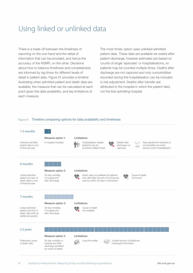
61 Spotlight on Measurement: Measuring 30-day mortality following hospitalisation bhi.nsw.gov.au
There is a trade-off between the timeliness of reporting on the one hand and the detail of information that can be provided, and hence the accuracy of the RSMR, on the other. Decisions about how to balance timeliness and completeness are informed by lag times for different levels of detail in patient data. Figure 51 provides a timeline illustrating when admitted patient and death data are available, the measure that can be calculated at each point given the data availability, and key limitations of each measure.
The most timely option uses unlinked admitted patient data. These data are available six weeks after patient discharge, however estimates are based on counts of single ‘episodes’ or hospitalisations, so patients may be counted multiple times. Deaths after discharge are not captured and only comorbidities recorded during the hospitalisation can be included in risk adjustment. Deaths after transfer are attributed to the hospital in which the patient died, not the first admitting hospital.
Using linked or unlinked data
Figure 51 Timeline comparing options for data availability and timeliness
4 months
LimitationsMeasure option 2
Death data not available for patients who died after the end of the financial year but within 30 days of admission
30-day mortality,in hospital andafter discharge
Cause of death not known?
Linked admitted patient and fact of death data to endof financial year
7 months
LimitationsMeasure option 3
Cause of death not available
30-day mortality,in hospital andafter discharge
Linked admitted patient and fact of death data (with an additional quarter)
LimitationsMeasure option 4
Long time delay Limited amount of additional meaningful information
30-day mortality, in hospital and after discharge (stratified by cause of death)
Preliminary causeof death data
2.5 years
LimitationsMeasure option 1
Hospitalisation-based (patients may be counted multiple times)
In-hospital mortality Deaths afterdischarge not captured
Risk adjustment restricted to comorbidities recorded during current hospitalisation
1.5 months
Unlinked admitted patient data to end of financial year

62Spotlight on Measurement: Measuring 30-day mortality following hospitalisation bhi.nsw.gov.au
C2-5*
C1-5
BNM-5
A-5
A-6A-1
C1-7*BM-1 BNM-1
BM-3
A-7
0.0
1.0
2.0
3.0
0 20 40 60 80 100 120 140
RS
MR
(obs
erve
d/ex
pect
ed)
Expected number of deaths within 30 days
95% higher limit90% higher limit90% lower limit95% lower limitHigher than expectedNo different than expectedLower than expected
C2-2*
C2-1
BNM-5BNM-3
BNM-2
BNM-4A-5
A-6 A-3A-1
C1-3BM-1
A-4A-2
0.0
1.0
2.0
3.0
0 20 40 60 80 100 120 140
RS
MR
(obs
erve
d/ex
pect
ed)
Expected number of deaths within 30 days
95% higher limit90% higher limit90% lower limit95% lower limitHigher than expectedNo different than expectedLower than expected
Figure 52 Ischaemic stroke 30-day risk-standardised mortality ratio, NSW public hospitals, July 2009 – June 2012
The inability to capture deaths after discharge but within the 30 days following admission is the most compelling shortcoming. Across five conditions, between 21% and 50% of deaths occurred after discharge (see page 63). Further, the proportion of deaths that occurred after discharge varied across the state’s hospitals. Among hospitals with at least 10 deaths within 30 days between July 2009 and June 2012, the percentage ranged between 18%–73% for acute myocardial infarction, 9%–64% for ischaemic stroke, 0%–67% for haemorrhagic stroke, 0%–93% for pneumonia and 24%–83% for hip fracture surgery. This means that limiting
analyses to unlinked data and in-hospital deaths only provides an unbalanced view of performance.
To examine the impact of reporting in-hospital deaths only in the calculation of RSMRs, comparative funnel plots were produced for ischaemic stroke for the period July 2009 – June 2012 using both unlinked and linked data (Figure 52). Out of 71 hospitals, five were outliers with both unlinked and linked data, six were outliers based on unlinked data but not on linked data, and nine were outliers based on linked data but not on unlinked data.
RSMRs based on unlinked data — deaths in hospital within 30 days of admission
RSMRs based on linked data — deaths in and out of hospital within 30 days of admission
* Hospitals with less than 50 patients. These hospitals would not be publicly reported.

63 Spotlight on Measurement: Measuring 30-day mortality following hospitalisation bhi.nsw.gov.au
The BHI reports on 30-day mortality define deaths from any cause within 30 days of admission as the primary outcome. These pages explore the value of using cause of death data to provide additional information on RSMRs.
Preliminary cause of death data are available approximately two and a half years after the end of a financial year. This means that using cause of death information has considerable consequences for the timeliness of reporting. The accuracy of the information has also been called into question.43
An alternative approach to waiting for cause of death data to become available is to restrict analyses to in-hospital mortality, on the assumption that deaths in hospital are more likely to be related to the condition of interest than deaths after discharge. However, if this option were adopted, between a fifth and half of all deaths would be excluded from the analysis, and the predictive power of the model would decrease (Figure 53). Furthermore, the proportion of deaths that occur after discharge varies substantially by hospital. A hospital that discharges patients prematurely may appear to perform better if deaths outside hospital are excluded.
To examine the extra insight generated from using cause of death data, cohorts from the 2009–12 period were re-analysed using cause of death data.
The underlying cause of death is defined as ‘the disease or injury which initiated the train of morbid events leading directly to death’44. The percentage of patients whose death was attributed to the same ICD-10 chapter for both principal diagnosis and underlying cause of death was only slightly higher among patients who died in hospital than among patients who died after discharge. Across five conditions, the difference ranged from 9 to 15 percentage points (Figure 53). The leading underlying causes of death in hospital and after discharge for the conditions, are shown in Figure 54.
Further analysis on the ischaemic stroke cohort showed that the distribution in cause of death for patients who died in hospital and after discharge was similar when stratified according to days post admission (Figure 55).
These results suggest that the 30-day window reduced the likelihood of including unrelated deaths. Fact of death data appear to be sufficiently specific for use in RSMR measures of hospital performance.
Relying on ‘fact of death’ or ‘cause of death’ information
Figure 53 Number of deaths within 30 days and percentage of deaths with the same ICD10 chapter for principal diagnosis and underlying cause of death, July 2009 – June 2012
Deaths within 30 daysUnderlying cause of death same
ICD10 chapter (%)
Condition In hospital After discharge In hospital After discharge
Acute myocardial infarction 1,530 676 81% 68%
Ischaemic stroke 1,307 589 89% 80%
Haemorrhagic stroke 1,513 410 82% 73%
Pneumonia 3,275 1,468 35% 20%
Hip fracture surgery 545 541 34% 22%

64Spotlight on Measurement: Measuring 30-day mortality following hospitalisation bhi.nsw.gov.au
Figure 54 Underlying cause of death (ICD-10 block) in hospital and after discharge, July 2009 – June 2012
Figure 55 Ischaemic stroke, cause of death in hospital and after discharge, days post admission, July 2009 – June 2012
0200400600800
1000
In After discharge In After discharge In After discharge
0-7 8-14 15-30
Num
ber
of d
eath
s
Days post admission
Other ICD-10 chapter Same ICD-10 chapter Same ICD-10 code
Leading cause of death in hospital % Leading cause of death out of hospital %
Acute myocardial infarction
I20-I25 Ischaemic heart diseases 74% I20-I25 Ischaemic heart diseases 54%
I30-I52 Other forms of heart disease 4% C00-C97 Malignant neoplasms 9%
E10-E14 Diabetes mellitus 3% I30-I52 Other forms of heart disease 7%
C00-C97 Malignant neoplasms 3% I60-I69 Cerebrovascular diseases 6%
N17-N19 Renal failure 2% E10-E14 Diabetes mellitus 5%
Subtotal 86% Subtotal 80%
Ischaemic stroke
I60-I69 Cerebrovascular diseases 66% I60-I69 Cerebrovascular diseases 60%
I30-I52 Other forms of heart disease 13% I30-I52 Other forms of heart disease 10%
I20-I25 Ischaemic heart diseases 8% I20-I25 Ischaemic heart diseases 8%
C00-C97 Malignant neoplasms 2% C00-C97 Malignant neoplasms 6%
E10-E14 Diabetes mellitus 2% E10-E14 Diabetes mellitus 5%
Subtotal 91% Subtotal 90%
Haemorrhagic stroke
I60-I69 Cerebrovascular diseases 75% I60-I69 Cerebrovascular diseases 64%
C00-C97 Malignant neoplasms 6% C00-C97 Malignant neoplasms 10%
V01-X59 Accidents* 4% V01-X59 Accidents* 7%
I30-I52 Other forms of heart disease 3% I30-I52 Other forms of heart disease 4%
I20-I25 Ischaemic heart diseases 3% I20-I25 Ischaemic heart diseases 3%
Subtotal 91% Subtotal 89%
Pneumonia
C00-C97 Malignant neoplasms 19% C00-C97 Malignant neoplasms 31%
J09-J18 Influenza and pneumonia 18% I20-I25 Ischemic heart diseases 9%
J40-J47 Chronic lower respiratory diseases 11% F00-F09 Organic mental disorders 9%
I30-I52 Other forms of heart disease 8% J40-J47 Chronic lower respiratory diseases 8%
I20-I25 Ischemic heart diseases 7% J09-J18 Influenza and pneumonia 7%
Subtotal 63% Subtotal 63%
Hip fracture surgery
V01-X59 Accidents* 32% V01-X59 Accidents* 21%
I20-I25 Ischaemic heart diseases 18% I20-I25 Ischaemic heart diseases 17%
I30-I52 Other forms of heart disease 7% F00-F09 Organic mental disorders 10%
J60-J70 Lung diseases due to external agents 5% I60-I69 Cerebrovascular diseases 9%
J40-J47 Chronic lower respiratory diseases 5% C00-C97 Malignant neoplasms 7%
Subtotal 67% Subtotal 64%
* Nearly all haemorrhagic stroke patients and hip fracture patients with accident as cause of death were further classified as fall or exposure to unspecified factor (95% haemorrhagic stroke, 99% hip fracture).
** Deaths within 30 days of admission. Percentages may not add up to subtotal due to rounding.

65 Spotlight on Measurement: Measuring 30-day mortality following hospitalisation bhi.nsw.gov.au
There are clear advantages in terms of precision and increased statistical power when analyses are based on three-year reporting periods. However there is a balance to be struck in terms of the frequency of public reports: too infrequent reporting risks not being reflective of current performance; too frequent reporting risks overwhelming the system and not allowing sufficient time between reporting periods for changes to be enacted and for improvements to be discernible.
Although the RSMR is the preferred option for measuring and assessing 30-day mortality following hospitalisation, the analyses on this page considered whether it would be reasonable and informative to supplement RSMRs with more regular calculations of unadjusted observed mortality rates.
Over time, hospitals’ observed rates tended to fluctuate more than the expected rates. For ischaemic stroke, the change in observed and expected rates from one three-year period to
the next between July 2000 and June 2015 was calculated for peer group A-C hospitals. The distributions of changes in the observed and expected rates show that the observed rate is more variable — with changes ranging from -13.4 to +12.8 percentage points — than the expected rate, with changes ranging from -4.4 to +2.4 percentage points. This suggests that the characteristics of patients presenting to each hospital did not vary markedly across measurement periods while observed mortality varied more over time (Figure 56).
Hospitals with higher observed rates tend to have higher RSMRs. Looking across five conditions for the 2009–12 period, there was generally a good correlation between the RSMR and the observed unadjusted mortality rate. The Pearson correlation coefficient ranged from moderate (0.64) for acute myocardial infarction to strong (0.95) for haemorrhagic stroke (Figure 57). In contrast, there was no evidence of a relationship between expected rates and RSMRs.
Comparing RSMRs and unadjusted mortality rates
Figure 56 Ischaemic stroke, distribution of percentage point change in observed and expected rates over five sets of three-year periods, July 2000 – June 2015 (Peer group A-C hospitals)
Observed rate Expected rate
0102030405060708090
100
-10 -8 -6 -4 -2 0 2 4 6 8 10
%
Percentage point change
0102030405060708090
100
-10 -8 -6 -4 -2 0 2 4 6 8 10
%
Percentage point change

66Spotlight on Measurement: Measuring 30-day mortality following hospitalisation bhi.nsw.gov.au
Figure 57 Five conditions, observed mortality rate (%) and risk-standardised mortality ratio, NSW public hospitals, July 2009 – June 2012
0
1
2
3
0 20 40 60 80 100
RS
MR
Observed rate
0
1
2
3
0 20 40 60 80 100R
SM
RObserved rate
0
1
2
3
0 20 40 60 80 100
RS
MR
Observed rate
0
1
2
3
0 20 40 60 80 100
RS
MR
Observed rate
0
1
2
3
0 20 40 60 80 100
RS
MR
Observed rate
0
1
2
3
0 20 40 60 80 100
RS
MR
Observed rate
0
1
2
3
0 20 40 60 80 100
RS
MR
Observed rate
0
1
2
3
0 20 40 60 80 100
RS
MR
Observed rate
0
1
2
3
0 20 40 60 80 100
RS
MR
Observed rate
0
1
2
3
0 20 40 60 80 100
RS
MR
Observed rate
0
1
2
3
0 20 40 60 80 100
RS
MR
Observed rate
0
1
2
3
0 20 40 60 80 100
RS
MR
Observed rate
0
1
2
3
0 20 40 60 80 100
RS
MR
Observed rate
0
1
2
3
0 20 40 60 80 100
RS
MR
Observed rate
0
1
2
3
0 20 40 60 80 100
RS
MR
Observed rate
Acute myocardial infarction
Pearson correlation coefficient = 0.64
95% confidence interval: 0.51-0.74
Pearson correlation coefficient = 0.95
95% confidence interval: 0.93-0.97
Pearson correlation coefficient = 0.94
95% confidence interval: 0.88-0.97
Pearson correlation coefficient = 0.91
95% confidence interval: 0.86-0.94
Pearson correlation coefficient = 0.82
95% confidence interval: 0.75-0.86
Haemorrhagic stroke
Hip fracture surgery
Ischaemic stroke
Pneumonia
Hospital RSMR results
Higher than expected
No different than expected
Lower than expected
* Data for hospitals with an expected mortality < 1.0 are suppressed.

67 Spotlight on Measurement: Measuring 30-day mortality following hospitalisation bhi.nsw.gov.au
RSMRs are a ratio of ‘observed’ deaths to ‘expected’ deaths. For each hospital, the number of expected deaths is calculated by a statistical model that takes account of its patients’ characteristics. Over time, the observed rate tends to fluctuate more than the expected rate (see page 65, Figure 56). This finding was explored for a sample of hospitals by plotting the three-year observed rate (deaths per 100 patients), expected rate and RSMR over time (Figure 58). In these plots, there is a strong association between movements in the observed rate and the RSMR, while the expected rate is relatively stable over time. Therefore, if a hospital’s RSMR changes substantially, it is likely because the observed rate (based on the number of deaths within 30 days), has changed rather than the expected rate (based on the model that accounts for case mix). This means that meaningful information can be provided to hospitals using a
mix of model-based, risk-adjusted RSMRs, publicly reported measures; as well as unadjusted observed mortality rates, for more frequent updates to support formative assessments locally. ‘Key’ diagrams that display unadjusted annual mortality data alongside the three-year RSMR are now being provided to hospitals by BHI (Figure 59). In these diagrams, the bars represent the difference between a hospital’s observed rate and the NSW observed rate for each of the years in the three-year period. The circle represents the three-year RSMR and is colour coded according to whether the hospital had higher than expected mortality (red), lower than expected mortality (green), or no different than expected (grey). These diagrams may help inform clinicians and managers about the relative contribution of each year’s results in their hospital’s three-year RSMR.
Hospital results: RSMRs and unadjusted rates

68Spotlight on Measurement: Measuring 30-day mortality following hospitalisation bhi.nsw.gov.au
-1.6
4.6
-1.7
-5.4-2.6 -3.6
0.0
0.4
0.8
1.2
1.6
2.0
2.4
0
5
10
15
20
25
July 00 –June 03
July 03 –June 06
July 06 –June 09
July 09 –June 12
July 12 –June 15
Obs
erve
d (u
nadj
uste
d) r
ate
Exp
ecte
d ra
te
Ris
k–st
anda
rdis
edm
orta
lity
ratio
(RS
MR
)
Statistically significant result Intermediate result
0.0
0.4
0.8
1.2
1.6
2.0
2.4
0
5
10
15
20
25
30
July 00 –June 03
July 03 –June 06
July 06 –June 09
July 09 –June 12
July 12 –June 15
Obs
erve
d (u
nadj
uste
d) r
ate
Exp
ecte
d ra
te
Ris
k–st
anda
rdis
edm
orta
lity
ratio
(RS
MR
)
Statistically significant result Intermediate result
0.0
0.2
0.4
0.6
0.8
1.0
1.2
1.4
0
5
10
15
20
25
July 00 –June 03
July 03 –June 06
July 06 –June 09
July 09 –June 12
July 12 –June 15
Obs
erve
d (u
nadj
uste
d) r
ate
Exp
ecte
d ra
te
Ris
k–st
anda
rdis
edm
orta
lity
ratio
(RS
MR
)
Statistically significant result Intermediate result
0.72.3
5.6
Unadjusted mortality rate percentage point difference from NSW result
RSMRJuly 2012 –June 2015
July 12 –June 13
July 13 –June 14
July 14 –June 15
Unadjusted mortality rate percentage point difference from NSW result
RSMRJuly 2012 –June 2015
July 12 –June 13
July 13 –June 14
July 14 –June 15
Unadjusted mortality rate percentage point difference from NSW result
RSMRJuly 2012 –June 2015
July 12 –June 13
July 13 –June 14
July 14 –June 15
Figure 58 Ischaemic stroke, observed rate, expected rate and RSMR for selected hospitals, three-year periods, July 2000 – June 2015
* While observed rates can provide hospitals with insights into performance, they should not be used to compare hospitals. Not adjusted for case mix or patient volume.
Hospital A-1
Hospital BNM-3
Hospital C1-3
0.7 2.3 5.6
Lower than expected
No different than expected
Higher than expected
RSMR:
Unadjusted mortality rate percentage point difference from NSW result
RSMR July 2012 – June 2015
July 12 – June 13
July 13 – June 14
July 14 – June 15
0.7 2.3 5.6
Lower than expected
No different than expected
Higher than expected
RSMR:
Unadjusted mortality rate percentage point difference from NSW result
RSMR July 2012 – June 2015
July 12 – June 13
July 13 – June 14
July 14 – June 15
0.7 2.3 5.6
Lower than expected
No different than expected
Higher than expected
RSMR:
Unadjusted mortality rate percentage point difference from NSW result
RSMR July 2012 – June 2015
July 12 – June 13
July 13 – June 14
July 14 – June 15
Figure 59 Ischaemic stroke ‘key’ diagrams, difference in hospital and NSW annual observed mortality rate and three-year RSMR for selected hospitals, July 2012 – June 2015

69 Spotlight on Measurement: Measuring 30-day mortality following hospitalisation bhi.nsw.gov.au
Public reporting of performance information has been shown to have a powerful effect on motivating change and supporting improvement at a hospital and clinician level.45,46 In public healthcare systems it is an important mechanism for providing accountability. However, public reporting on hospital performance requires judicious application.
While the frequency of reporting RSMR results is, to a large extent, shaped by the measurement period used in the analysis, there are other factors to consider in determining reporting schedules. These include the availability of resources to review and respond to RSMRs at a local and system level, and the need to allow sufficient time between reporting periods for any changes put in place to take effect. There is a balance to be struck between providing information on a sufficiently regular basis so as to guide and inform improvement efforts on the one hand, and yet not overwhelm organisations and clinicians with too frequent public releases of information on the other.
Some organisations use a mixed reporting approach to resolve these tensions. England’s Health & Social Care Information Centre (HSCIC) publicly reports rolling annual mortality measures every quarter but only highlights those hospitals that are outliers both in the current period and in the same quarter in the previous year.8 In this way, hospitals are assessed on two non-overlapping periods, avoiding unfair
criticism of a hospital that continues to be an outlier on quarterly mortality results when they have not had time to improve, or they have improved but the earlier poor performance is still influencing the rolling average. In a NSW context however, given smaller volumes, quarterly reporting is not possible.
A mixed reporting approach is also used by the Australian Bureau of Statistics, with the release of preliminary death data in a timely way followed by revised and final figures when more complete data and analyses are available.47
BHI’s public reports that assess hospital performance are rigorous and impartial. As well as descriptive statistics, reports often contain sophisticated statistical analyses that take account of patient characteristics and hospital case mix. This supports summative asessments that are fair and reflect differences in the care provided. Such risk-standardised analyses can however be time consuming.
The results of the analyses in this edition of Spotlight on Measurement reaffirm that unadjusted rates are sufficiently accurate to support formative assessments of performance by local healthcare providers. This means that more timely data can be released to guide improvement, while more robust risk-adjustment processes can be reserved for less frequent public reports.
Conclusion

70Spotlight on Measurement: Measuring 30-day mortality following hospitalisation bhi.nsw.gov.au


Appendices

73 Spotlight on Measurement: Measuring 30-day mortality following hospitalisation bhi.nsw.gov.au
Appendix 1: Peer groups
NSW hospitals vary in size and in the types and complexity of clinical services that they provide. It is important to compare similar or like hospitals. To do this, BHI uses a NSW Health Classification system called ‘peer group’ (Figure A1.1).
Group Name Description
A Principal referralVery large hospitals providing a broad range of services, including specialised units at a state or national level (for this report, ungrouped tertiary hospitals are included in this group)
BM/BNM Major Large metropolitan (BM) and non-metropolitan (BNM) hospitals
C1 District group 1 Medium-sized hospitals treating between 5,000–10,000 patients annually
C2 District group 2 Smaller hospitals, typically in rural locations
D-F CommunityCommunity, nursing home, multipurpose, palliative care and rehabilitation facilities
Figure A1.1 NSW public hospitals peer group classification used in this report

74Spotlight on Measurement: Measuring 30-day mortality following hospitalisation bhi.nsw.gov.au
Appendix 2: Funnel plotsInterpreting funnel plots
Funnel plots are used to compare individual hospital performance to a NSW benchmark. The aim is to identify hospitals with more variation than expected due to chance alone; so called special cause variability.35 Mortality ratios are plotted against the expected number of deaths, and hospitals lying outside the quality control limits are flagged as requires further investigation or intervention.
Random variability in mortality ratios is expected for all hospitals. The amount of variation depends on the patient load, so smaller hospitals are more variable. The distribution of mortality ratios, if the only source of variation is chance, is assumed known.35 This is called the ‘null distribution’. Using the null distribution, control limits are constructed within which a nominal amount of observed mortality ratios will fall on average, provided that hospitals only vary by chance. In practice 95% and 99.8% coverage is used to construct control limits. Hospitals falling outside these limits may have unwarranted clinical variation and require further investigation.
0
1
2
3
0 20 40 60 80 100 120 140 160 180 200 220
Ris
k-st
anda
rdis
ed m
orta
lity
ratio
(RS
MR
)
Expected number of deaths within 30 days
99.8% limits 95.0% limits
Higher than expected:
No different than expected:
Lower than expected:
This hospital
Peer hospitals
Other hospitals
Hospital with higher mortality
Hospital with lower mortality
Hospital within the range of values expected for an in control NSW hospital (inside the funnel)
Hospital with higher mortality (between 95% and 99.8% control limits)
Greater tolerance for variation for hospitals with fewer
expected deaths Reflects patient volume and
case mix at the hospital
Figure A2.1 How to interpret a funnel plot
Using this method of constructing control limits, the question being asked is, ‘Acknowledging that there are differences among hospitals, which hospitals are probably extraordinary performers?’ 48
The funnel shape that gives the funnel plots its name shows the distribution of tolerable random variation around the NSW benchmark (Figure A2.1). Hospitals with lower than expected mortality have greater chance variability and fair judgements about performance should take this into account. Hospitals above the 95% limit are considered to have mortality higher than expected given case mix and chance variation. Hospitals below the 95% limit are considered to have mortality lower than expected given case mix and chance variation.
It is possible that a hospital falls outside the limits solely due to chance. Using 95% coverage, it is expected that one hospital in 40 that is only varying by chance will fall above the upper control limit. Using 99.8% coverage, it is expected that one hospital in 1,000 that is varying by chance alone will fall above the upper control limit. Therefore for hospitals outside the 99.8% limits, there is greater confidence about them having special cause variability.
75 Spotlight on Measurement: Measuring 30-day mortality following hospitalisation bhi.nsw.gov.au
Statistical properties of control limits
It is assumed that 30-day mortality counts, at hospitals varying only by chance, arise from a Poisson process. Because the Poisson is a discrete distribution, probabilities only exist for integer values. However, expected mortality can take non-integer values such as 3.4, so when constructing control limits, probabilities between integer values are interpolated.35 This turns the control limit from a step function into a smooth line.
Nominal coverage areas are only ‘true’ on average. For any period of data, the true coverage between the control limits will vary from the nominal level. For example, three out of 80 hospitals could fall above the 95% upper limit by chance alone in an unlucky period when two out of 80 are expected.
Nominal coverage areas are only unbiased for large hospitals. For smaller hospitals, the true coverage is biased upwards, and therefore higher than nominal coverage. For example, if the nominal coverage is set at 95%, then for small hospitals true coverage is about 98% on average.49 Note that the best known method to construct limits is used, but no method is perfect. Also only results for larger hospitals are reported which reduces the effect of this bias (hospitals must have at least 50 patients from the condition cohort, and be in peer groups A, B, or C).
Control limit methods do not account for uncertainty in the NSW baseline rate, and this could bias results in either direction.50 However, BHI uses a relatively large number of patients to estimate the baseline rate, so the uncertainty will be negligible. There is a way to set control limits that accounts for uncertainty in the baseline, but it can be too conservative.50
No correction has been made for multiple comparisons, aside from the usage of a very large coverage area,35 which is consistent with other jurisdictions.
The probability of being flagged as having excess variation depends on three key factors:51
1. The magnitude of clinical variation. A hospital with greater divergence from the baseline is more likely to be flagged.
2. Patient load. Random variation is lower in larger centres, increasing the power to spot systematic variation.
3. The rarity of death. The number of expected deaths is lower for less serious conditions, so the random variation is higher, and there is less power to spot true differences in mortality ratios.
Taken together, these factors mean that truly errant small hospitals are unlikely to be identified, but unwarranted variation in larger hospitals is more likely to be spotted.
Appendix 2: Funnel plots continued

76Spotlight on Measurement: Measuring 30-day mortality following hospitalisation bhi.nsw.gov.au
Statistical properties of baselines
The baseline in a funnel plot is the central line around which control limits are placed. The baseline can be a performance target, or national or state average, and can be calculated using historical or contemporary data. It is often stated that the baseline is 1, by definition.51-53 However, this is only true when the prediction model used to calculate expected counts is derived from the same dataset as that containing the current observed counts, and certain methods of modelling and risk-standardised mortality ratio (RSMR) derivation are used. For example, in a teen-pregnancy study,54 results are presented for 2004, but the model used to predict expected counts was constructed using historical data from the late 1990s.55 As the rate of teen pregnancy has been falling since the period used for modelling, the overall expected count is higher than the observed count, and the baseline RSMR is less than one.
For the funnel plots in BHI reports on 30-day mortality, the baseline is often very close to one, but because of the model and RSMR used, the baseline can be different from one. If the baseline was substantially lower than one, a hospital could have a RSMR lower than one and still be flagged as having excessive mortality. This apparent contradiction is due to the conflation of two interpretations. The RSMR compares observed mortality at a hospital to the expected mortality if those patients were treated at the average hospital.56 If a hospital RSMR is above 1, then they have higher mortality than we would expect if their patient case mix were treated at the average hospital. If a hospital is above the upper funnel plot control limit, it is varying from the NSW average more than would be expected by chance alone.
There are methods to scale RSMRs so that they are centred at one, but they make the methodology more complicated and results are harder to interpret.52

77 Spotlight on Measurement: Measuring 30-day mortality following hospitalisation bhi.nsw.gov.au
Appendix 3: Acute myocardial infarction indicator specification RSMR indicator specification, cohort and prediction model
The condition
An acute myocardial infarction (AMI), or heart attack, occurs when the blood supply to part of the heart is interrupted, resulting in death of heart cells. The heart muscle suffers permanent damage if blood supply is not restored quickly.
The indicator
The RSMR provides a fair comparison of a particular hospital’s results in deaths in or out of hospital within 30 days of admission given, its case mix with an average NSW hospital with the same case mix.6
Data source
Data were drawn from the NSW Admitted Patient Data Collection and NSW Registry of Births, Deaths and Marriages, and were probabilistically linked by the Centre for Health Record Linkage. Data access was via SAPHaRI, Centre for Epidemiology and Evidence, NSW Ministry of Health. SAS and StataSE v12 were used for the analyses.
Calculation
The ratio of the observed number of deaths (numerator) to the expected number of deaths (denominator) in or out of hospital within 30 days of admission for AMI at a given hospital.
Cohort index admissions
An index admission is the hospitalisation included in calculating RSMRs for the condition of interest. The index admissions form the ‘cohort’ for assessing 30-day mortality.
Inclusions
• Principal diagnosis of AMI (ICD-10-AM code I21)
• Aged 15 years or over
• Acute, emergency admissions
• Discharged between 1 July 2012 and 30 June 2015.
Exclusions
• Discharges from NSW hospitals administered by agencies external to NSW
• Patients with hospitalisations coded as ‘STEMI, not specified’ (ICD-10-AM I21.9) were excluded from the base model and analysed separately.
Period of care and transfers
Multiple acute, contiguous hospitalisations were considered as a single, acute period of care. Acute admissions on the same day of separation from another acute hospitalisation were included in the same acute period of care, regardless of the mode of separation recorded in the initial hospital. If an acute admission is coded as ending in a transfer, and there is another acute admission within one day of that transfer, the second admission is concatenated into the same period of care. For patients who had multiple periods of care for a condition, only the last period of care was considered in the analysis for that condition.
78Spotlight on Measurement: Measuring 30-day mortality following hospitalisation bhi.nsw.gov.au
Numerator
Observed number of deaths in or out of hospital within 30 days of admission for AMI.
Denominator
Expected number of deaths at a given hospital, on the basis of an average NSW hospital’s performance with the same case mix, calculated as the sum of the estimated probabilities of deaths using a NSW-level prediction model.
Attribution of index admissions and deaths
In cases of patient transfers, index admissions and deaths are attributed to the first admitting hospital within the period of care.
Development and validation of the prediction model
The NSW-level prediction model was developed using index admissions between 1 July 2009 and 30 June 2012 and using random intercept logistic regression models, taking into account patient-level risk factors (age, sex and comorbidities) and clustering within hospitals.54 A backward modelling approach was used to build the multivariable regression model. Variables significant at the 0.20 level in the univariable analysis were considered for inclusion in the multivariable model. Only variables with a 2-sided p-value of less than 0.05 in the multivariable model were retained in the final model.
The prediction ability of the model was assessed using c-statistics in data from other financial years. The stability of the coefficients in other financial years was also tested. The clinical relevance of the variables in the final model and their direction of association with the outcome were reviewed by clinicians.
The model coefficients were recalibrated using index admissions between 1 July 2012 and 30 June 2015 to calculate the expected mortality for each hospital during that period.
Risk adjustment variables
The following variables are included in the development of the prediction models:
• Age at index admission
• Sex
• The Australian Commission on Safety and Quality in Health Care comorbidity list,57 with a one-year look back period in hospital data.
The final set of risk-adjustment variables for AMI were: age, STEMI/non-STEMI status, dementia, Alzheimer’s disease, hypotension, shock, renal failure, heart failure, dysrhythmia, malignancy, hypertension and cerebrovascular disease.
Presentation
Results are presented in a funnel plot. Hospitals with an RSMR that falls beyond the 95% and 99.8% control limits are flagged. Control limits are calculated based on a Poisson distribution.35

79 Spotlight on Measurement: Measuring 30-day mortality following hospitalisation bhi.nsw.gov.au
Appendix 3: Acute myocardial infarction indicator specification continued
Figure A3.1 Acute myocardial infarction prediction model for deaths in or out of hospital within 30 days, July 2009 – June 2012
Figure A3.2 Acute myocardial infarction model performance (c-statistics) over different time periods
Predictors Odds Ratio P-value (95% confidence interval)
Age (per year increase) 1.06 <0.001 (1.05 - 1.06)
Age squared 1.00 <0.001 (1.00 - 1.00)
STEMI 2.69 <0.001 (2.42 - 3.00)
Dementia 1.91 <0.001 (1.59 - 2.30)
Alzheimer’s disease 1.59 0.031 (1.04 - 2.42)
Hypotension 1.29 <0.001 (1.14 - 1.45)
Shock 9.40 <0.001 (7.80 - 11.34)
Renal failure 2.34 <0.001 (2.08 - 2.62)
Heart failure 1.78 <0.001 (1.60 - 1.99)
Dysrhythmia 1.71 <0.001 (1.54 - 1.90)
Malignancy 2.35 <0.001 (1.91 - 2.89)
Hypertension 0.67 <0.001 (0.61 - 0.74)
Cerebrovascular disease 2.29 <0.001 (1.90 - 2.75)
Period c-statistic
July 2012 – June 2015 0.85
July 2009 – June 2012 0.85
July 2006 – June 2009 0.83
July 2003 – June 2006 0.85

80Spotlight on Measurement: Measuring 30-day mortality following hospitalisation bhi.nsw.gov.au
Figure A3.3 Acute myocardial infarction model coefficient stability, four time periods, July 2003 – June 2015
-1.0
-0.5
0.0
0.5
1.0
1.5
2.0
2.5
3.0
Coe
ffici
ent
July 2003-June 2006 July 2006-June 2009 July 2009-June 2012 July 2012-June 2015

81 Spotlight on Measurement: Measuring 30-day mortality following hospitalisation bhi.nsw.gov.au
Appendix 4: Ischaemic stroke indicator specification RSMR indicator specification, cohort and prediction model
The condition
Ischaemic stroke occurs when a blood vessel is blocked depriving the brain of oxygen and nutrients. As a result, the area of the brain supplied or drained by the blood vessel suffers damage. The severity and consequences of stroke can vary from complete recovery to severe disability or death.
The indicator
The RSMR provides a fair comparison of a particular hospital’s results in deaths in or out of hospital within 30 days of admission, given its case mix with an average NSW hospital with the same case mix.6
Data source
Data were drawn from the NSW Admitted Patient Data Collection and NSW Registry of Births, Deaths and Marriages, and were probabilistically linked by the Centre for Health Record Linkage. Data access was via SAPHaRI, Centre for Epidemiology and Evidence, NSW Ministry of Health. SAS and StataSE v12 were used for the analyses.
Calculation
The ratio of the observed number of deaths (numerator) to the expected number of deaths (denominator) in or out of hospital within 30 days of admission for ischaemic stroke at a given hospital.
Cohort index admissions
An index admission is the hospitalisation included in calculating RSMRs for the condition of interest. The index admissions form the ‘cohort’ for assessing 30-day mortality.
Inclusions
• Principal diagnosis of ischaemic stroke (ICD-10-AM code I63)
• Aged 15 years or over
• Acute, emergency admissions
• Discharged between 1 July 2012 and 30 June 2015.
Exclusions
• Discharges from NSW hospitals administered by agencies external to NSW.
Period of care and transfers
Multiple acute, contiguous hospitalisations were considered as a single, acute period of care. Acute admissions on the same day of separation from another acute hospitalisation were included in the same acute period of care, regardless of the mode of separation recorded in the initial hospital. If an acute admission is coded as ending in a transfer, and there is another acute admission within one day of that transfer, the second admission is concatenated into the same period of care. For patients who had multiple periods of care for a condition, only the last period of care was considered in the analysis for that condition.
Numerator
Observed number of deaths in or out of hospital within 30 days of admission for ischaemic stroke.
Denominator
Expected number of deaths at a given hospital, on the basis of an average NSW hospital’s performance with the same case mix, calculated as the sum of the estimated probabilities of deaths using a NSW-level prediction model.

82Spotlight on Measurement: Measuring 30-day mortality following hospitalisation bhi.nsw.gov.au
Risk adjustment variables
The following variables are included in the development of the prediction models:
• Age at index admission
• Sex
• The Australian Commission on Safety and Quality in Health Care comorbidity list,57 with a one-year look back period in hospital data.
The final set of risk-adjustment variables for ischaemic stroke were: age, sex, renal failure, heart failure, and malignancy.
Presentation
Results are presented in a funnel plot. Hospitals with an RSMR that falls beyond the 95% and 99.8% control limits are flagged. Control limits are calculated based on a Poisson distribution.35
Attribution of index admissions and deaths
In cases of patient transfers, index admissions and deaths are attributed to the first admitting hospital within the period of care.
Development and validation of the prediction model
The NSW-level prediction model was developed using index admissions between 1 July 2009 and 30 June 2012 and using random intercept logistic regression models, taking into account patient-level risk factors (age, sex and comorbidities) and clustering within hospitals.54 A backward modelling approach was used to build the multivariable regression model. Variables significant at the 0.20 level in the univariable analysis were considered for inclusion in the multivariable model. Only variables with a 2-sided p-value of less than 0.05 in the multivariable model were retained in the final model.
The prediction ability of the model was assessed using c-statistics in data from other financial years. The stability of the coefficients in other financial years was also tested. The clinical relevance of the variables in the final model and their direction of association with the outcome were reviewed by clinicians.
The model coefficients were recalibrated using index admissions between 1 July 2012 and 30 June 2015 to calculate the expected mortality for each hospital during that period.

83 Spotlight on Measurement: Measuring 30-day mortality following hospitalisation bhi.nsw.gov.au
Figure A4.1 Ischaemic stroke prediction model for deaths in or out of hospital within 30 days, July 2009 – June 2012
Figure A4.2 Ischaemic stroke model performance (c-statistics) over different time periods
Figure A4.3 Ischaemic stroke model coefficient stability, four time periods, July 2003 – June 2015
Predictors Odds Ratio P-value (95% confidence interval)
Age (per year increase) 1.06 <0.001 (1.06 - 1.07)
Age squared 1.00 <0.001 (1.00 - 1.00)
Female 1.30 <0.001 (1.17 - 1.44)
Renal failure 1.68 <0.001 (1.45 - 1.94)
Heart failure 1.98 <0.001 (1.69 - 2.32)
Malignancy 2.69 <0.001 (2.19 - 3.30)
Period c-statistic
July 2012 – June 2015 0.75
July 2009 – June 2012 0.74
July 2006 – June 2009 0.73
July 2003 – June 2006 0.72
-1.0
-0.5
0.0
0.5
1.0
1.5
2.0
2.5
Coe
ffici
ent
July 2003-June 2006 July 2006-June 2009 July 2009-June 2012 July 2012-June 2015
Appendix 4: Ischaemic stroke indicator specification continued

84Spotlight on Measurement: Measuring 30-day mortality following hospitalisation bhi.nsw.gov.au
Appendix 5: Haemorrhagic stroke indicator specificationRSMR indicator specification, cohort and prediction model
The condition
Haemorrhagic stroke occurs when a blood vessel, usually an artery, develops a leak or bursts. Consequently, the brain surrounding the vessel is damaged by blood or pressure. The severity and consequences of stroke can vary from complete recovery to severe disability or death.
The indicator
The RSMR provides a fair comparison of a particular hospital’s results in deaths in or out of hospital within 30 days of admission, given its case mix with an average NSW hospital with the same case mix.6
Data source
Data were drawn from the NSW Admitted Patient Data Collection and NSW Registry of Births, Deaths and Marriages, and were probabilistically linked by the Centre for Health Record Linkage (CheReL). Data access was via SAPHaRI, Centre for Epidemiology and Evidence, NSW Ministry of Health. SAS and StataSE v12 were used for the analyses.
Calculation
The ratio of the observed number of deaths (numerator) to the expected number of deaths (denominator) in or out of hospital within 30 days of admission for haemorrhagic stroke at a given hospital.
Cohort index admissions
An index admission is the hospitalisation included in calculating RSMRs for the condition of interest. The index admissions form the ‘cohort’ for assessing 30-day mortality.
Inclusions
• Principal diagnosis of haemorrhagic stroke (ICD-10-AM codes I61, I62)
• Aged 15 years or over
• Acute, emergency admissions
• Discharged between 1 July 2012 and 30 June 2015.
Exclusions
Discharges from NSW hospitals administered by agencies external to NSW.
Period of care and transfers
Multiple acute, contiguous hospitalisations were considered as a single, acute period of care. Acute admissions on the same day of separation from another acute hospitalisation were included in the same acute period of care, regardless of the mode of separation recorded in the initial hospital. If an acute admission is coded as ending in a transfer, and there is another acute admission within one day of that transfer, the second admission is concatenated into the same period of care. For patients who had multiple periods of care for a condition, only the last period of care was considered in the analysis for that condition.
Numerator
Observed number of deaths in or out of hospital within 30 days of admission for haemorrhagic stroke.
Denominator
Expected number of deaths at a given hospital, on the basis of an average NSW hospital’s performance with the same case mix, calculated as the sum of the estimated probabilities of deaths using a NSW-level prediction model.
Attribution of index admissions and deaths
In cases of patient transfers, index admissions and deaths are attributed to the first admitting hospital within the period of care.

85 Spotlight on Measurement: Measuring 30-day mortality following hospitalisation bhi.nsw.gov.au
Appendix 5: Haemorrhagic stroke indicator specification continued
Development and validation of the prediction model
The NSW-level prediction model was developed using index admissions between 1 July 2009 and 30 June 2012 and using random intercept logistic regression models, taking into account patient-level risk factors (age, sex and comorbidities) and clustering within hospitals.54 A backward modelling approach was used to build the multivariable regression model. Variables significant at the 0.20 level in the univariable analysis were considered for inclusion in the multivariable model. Only variables with a 2-sided p-value of less than 0.05 in the multivariable model were retained in the final model.
The prediction ability of the model was assessed using c-statistics in data from other financial years. The stability of the coefficients in other financial years was also tested. The clinical relevance of the variables in the final model and their direction of association with the outcome were reviewed by clinicians.
The model coefficients were recalibrated using index admissions between 1 July 2012 and 30 June 2015 to calculate the expected mortality for each hospital during that period.
Risk adjustment variables
The following variables are included in the development of the prediction models:
• Age at index admission
• Sex
• The Australian Commission on Safety and Quality in Health Care comorbidity list,57 with a one-year look back period in hospital data.
The final set of risk-adjustment variables for haemorrhagic stroke were: age, sex, heart failure, malignancy and history of haemorrhagic stroke.
Presentation
Results are presented in a funnel plot. Hospitals with an RSMR that falls beyond the 95% and 99.8% control limits are flagged. Control limits are calculated based on a Poisson distribution.35

86Spotlight on Measurement: Measuring 30-day mortality following hospitalisation bhi.nsw.gov.au
Figure A5.1 Haemorrhagic stroke prediction model for deaths in or out of hospital within 30 days, July 2009 – June 2012
Figure A5.2 Haemorrhagic stroke model performance (c-statistics) over different time periods
Figure A5.3 Haemorrhagic stroke model coefficient stability, four time periods, July 2003 – June 2015
Predictors Odds Ratio P-value (95% confidence interval)
Age (per year increase) 1.04 <0.001 (1.03 - 1.04)
Female 1.38 <0.001 (1.23 - 1.55)
Previous haemorrhagic stroke 0.63 <0.001 (0.50 - 0.80)
Heart failure 1.60 <0.001 (1.26 - 2.03)
Malignancy 2.72 <0.001 (2.17 - 3.41)
Period c-statistic
July 2012 – June 2015 0.66
July 2009 – June 2012 0.68
July 2006 – June 2009 0.69
July 2003 – June 2006 0.66
-1.0
-0.5
0.0
0.5
1.0
1.5
2.0
2.5
Coe
ffici
ent
July 2003-June 2006 July 2006-June 2009 July 2009-June 2012 July 2012-June 2015

87 Spotlight on Measurement: Measuring 30-day mortality following hospitalisation bhi.nsw.gov.au
Appendix 6: Congestive heart failure indicator specificationRSMR indicator specification, cohort and prediction model
The condition
Congestive heart failure is a chronic condition that occurs when the heart is unable to keep up with the demands of, or provide adequate blood flow to other organs. It often develops as a result of hypertension, diabetes or other coronary diseases.
The indicator
The RSMR provides a fair comparison of a particular hospital’s results in deaths in or out of hospital within 30 days of admission, given its case mix with an average NSW hospital with the same case mix.6
Data source
Data were drawn from the NSW Admitted Patient Data Collection and NSW Registry of Births, Deaths and Marriages, and were probabilistically linked by the Centre for Health Record Linkage. Data access was via SAPHaRI, Centre for Epidemiology and Evidence, NSW Ministry of Health. SAS and StataSE v12 were used for the analyses.
Calculation
The ratio of the observed number of deaths (numerator) to the expected number of deaths (denominator) in or out of hospital within 30 days of admission for congestive heart failure at a given hospital.
Cohort index admissions
An index admission is the hospitalisation included in calculating RSMRs for the condition of interest. The index admissions form the ‘cohort’ for assessing 30-day mortality.
Inclusions
• Principal diagnosis of congestive heart failure (ICD-10-AM codes I11.0, I13.0, I13.2, I50.0, I50.1, I50.9)
• Aged 45 years or over
• Acute, emergency admissions
• Discharged between 1 July 2012 and 30 June 2015.
Exclusions
• Discharges from NSW hospitals administered by agencies external to NSW.
Period of care and transfers
Multiple acute, contiguous hospitalisations were considered as a single, acute period of care. Acute admissions on the same day of separation from another acute hospitalisation were included in the same acute period of care, regardless of the mode of separation recorded in the initial hospital. If an acute admission is coded as ending in a transfer, and there is another acute admission within one day of that transfer, the second admission is concatenated into the same period of care. For patients who had multiple periods of care for a condition, only the last period of care was considered in the analysis for that condition.
Numerator
Observed number of deaths in or out of hospital within 30 days of admission for congestive heart failure.
Denominator
Expected number of deaths at a given hospital, on the basis of an average NSW hospital’s performance with the same case mix, calculated as the sum of the estimated probabilities of deaths using a NSW-level prediction model.

88Spotlight on Measurement: Measuring 30-day mortality following hospitalisation bhi.nsw.gov.au
Attribution of index admissions and deaths
In cases of patient transfers, index admissions and deaths are attributed to the first admitting hospital within the period of care.
Development and validation of the prediction model
The NSW-level prediction model was developed using index admissions between 1 July 2009 and 30 June 2012 and using random intercept logistic regression models, taking into account patient-level risk factors (age, sex and comorbidities) and clustering within hospitals.54 A backward modelling approach was used to build the multivariable regression model. Variables significant at the 0.20 level in the univariable analysis were considered for inclusion in the multivariable model. Only variables with a 2-sided p-value of less than 0.05 in the multivariable model were retained in the final model.
The prediction ability of the model was assessed using c-statistics in data from other financial years. The stability of the coefficients in other financial years was also tested. The clinical relevance of the variables in the final model and their direction of association with the outcome were reviewed by clinicians.
The model coefficients were recalibrated using index admissions between 1 July 2012 and 30 June 2015 to calculate the expected mortality for each hospital during that period.
Risk adjustment variables
The following variables are included in the development of the prediction models:
• Age at index admission
• Sex
• Elixhauser comorbidities,58 with a one-year look back period in hospital data.
The final set of risk-adjustment variables for congestive heart failure were: age, sex, valvular disease, pulmonary circulation disorders, peripheral vascular disorder, hypertension, paralysis, other neurological disorders, chronic pulmonary disease, diabetes - complicated, renal failure, liver disease, lymphoma, metastatic cancer, coagulopathy, weight loss, fluid and electrolyte disorders, deficiency anaemia and number of previous acute admissions for congestive heart failure.
Presentation
Results are presented in a funnel plot. Hospitals with an RSMR that falls beyond the 95% and 99.8% control limits are flagged. Control limits are calculated based on a Poisson distribution.35

89 Spotlight on Measurement: Measuring 30-day mortality following hospitalisation bhi.nsw.gov.au
Appendix 6: Congestive heart failure indicator specification continued
Figure A6.1 Congestive heart failure prediction model for deaths in or out of hospital within 30 days, July 2009 – June 2012
Predictors Odds Ratio P-value (95% confidence interval)
Number of previous acute admissions CHF* (versus zero)
One 1.37 <0.001 (1.25 - 1.51)
Two 1.63 <0.001 (1.41 - 1.89)
Three or more 2.39 <0.001 (2.03 - 2.81)
Age (per year increase) 1.05 <0.001 (1.05 - 1.06)
Age squared 1.00 0.001 (1.00 - 1.00)
Female 0.90 0.009 (0.84 - 0.98)
Valvular disease 1.13 0.012 (1.03 - 1.25)
Pulmonary circulation disorders 1.19 0.002 (1.07 - 1.32)
Peripheral vascular disorder 1.20 0.008 (1.05 - 1.38)
Hypertension 0.83 <0.001 (0.77 - 0.90)
Paralysis 1.71 <0.001 (1.39 - 2.11)
Other neurological disorders 1.65 <0.001 (1.39 – 1.97)
Chronic pulmonary disease 1.25 <0.001 (1.15 – 1.37)
Diabetes, complicated 1.14 0.009 (1.03 - 1.25)
Renal failure 1.84 <0.001 (1.69 - 2.00)
Liver disease 2.74 <0.001 (2.25 - 3.33)
Lymphoma 2.17 <0.001 (1.51 - 3.09)
Metastatic cancer 3.16 <0.001 (2.50 – 3.98)
Coagulopathy 1.27 <0.001 (1.12 - 1.43)
Weight loss 1.56 <0.001 (1.38 - 1.76)
Fluid and electrolyte disorders 1.53 <0.001 (1.41 - 1.66)
Deficiency anaemia 0.77 <0.001 (0.67 - 0.88)
* Contiguous hospitalisation episodes for CHF are counted once; acute episodes with a principal diagnosis of CHF are considered.

90Spotlight on Measurement: Measuring 30-day mortality following hospitalisation bhi.nsw.gov.au
Figure A6.2 Congestive heart failure model performance (c-statistics) over different time periods
Figure A6.3 Congestive heart failure model coefficient stability, four time periods, July 2003 – June 2015
Period c-statistic
July 2012 – June 2015 0.71
July 2009 – June 2012 0.72
July 2006 – June 2009 0.70
July 2003 – June 2006 0.70
-1.0
-0.5
0.0
0.5
1.0
1.5
2.0
2.5
eNumb
viou
er
of pr
s
admiss
ions
CHF
Coe
ffici
ent
July 2003-June 2006 July 2006-June 2009 July 2009-June 2012 July 2012-June 2015

91 Spotlight on Measurement: Measuring 30-day mortality following hospitalisation bhi.nsw.gov.au
Appendix 7: Pneumonia indicator specificationRSMR indicator specification, cohort and prediction model
The condition
Pneumonia is an inflammatory condition of one or both lungs, usually due to infection. Symptoms may include fever, chills, cough with sputum production, chest pain, and shortness of breath.
The indicator
The RSMR provides a fair comparison of a particular hospital’s results in deaths in or out of hospital within 30 days of admission, given its case mix with an average NSW hospital with the same case mix.6
Data source
Data were drawn from the NSW Admitted Patient Data Collection and NSW Registry of Births, Deaths and Marriages, and were probabilistically linked by the Centre for Health Record Linkage. Data access was via SAPHaRI, Centre for Epidemiology and Evidence, NSW Ministry of Health. SAS and StataSE v12 were used for the analyses.
Calculation
The ratio of the observed number of deaths (numerator) to the expected number of deaths (denominator) in or out of hospital within 30 days of admission for pneumonia at a given hospital.
Cohort index admissions
An index admission is the hospitalisation included in calculating RSMRs for the condition of interest. The index admissions form the ‘cohort’ for assessing 30-day mortality.
Inclusions
• Principal diagnosis of pneumonia (ICD-10-AM codes J13, J14, J15, J16, J18)
• Aged 18 years or over
• Acute, emergency admissions
• Discharged between 1 July 2012 and 30 June 2015.
Exclusions
• Discharges from NSW hospitals administered by agencies external to NSW.
Period of care and transfers
Multiple acute, contiguous hospitalisations were considered as a single, acute period of care. Acute admissions on the same day of separation from another acute hospitalisation were included in the same acute period of care, regardless of the mode of separation recorded in the initial hospital. If an acute admission is coded as ending in a transfer, and there is another acute admission within one day of that transfer, the second admission is concatenated into the same period of care. For patients who had multiple periods of care for a condition, only the last period of care was considered in the analysis for that condition.
Numerator
Observed number of deaths in or out of hospital within 30 days of admission for pneumonia.
Denominator
Expected number of deaths at a given hospital, on the basis of an average NSW hospital’s performance with the same case mix, calculated as the sum of the estimated probabilities of deaths using a NSW-level prediction model.

92Spotlight on Measurement: Measuring 30-day mortality following hospitalisation bhi.nsw.gov.au
Attribution of index admissions and deaths
In cases of patient transfers, index admissions and deaths are attributed to the first admitting hospital within the period of care.
Development and validation of the prediction model
The NSW-level prediction model was developed using index admissions between 1 July 2009 and 30 June 2012 and using random intercept logistic regression models, taking into account patient-level risk factors (age, sex and comorbidities) and clustering within hospitals.54 A backward modelling approach was used to build the multivariable regression model. Variables significant at the 0.20 level in the univariable analysis were considered for inclusion in the multivariable model. Only variables with a 2-sided p-value of less than 0.05 in the multivariable model were retained in the final model.
The prediction ability of the model was assessed using c-statistics in data from other financial years. The stability of the coefficients in other financial years was also tested. The clinical relevance of the variables in the final model and their direction of association with the outcome were reviewed by clinicians.
The model coefficients were recalibrated using index admissions between 1 July 2012 and 30 June 2015 to calculate the expected mortality for each hospital during that period.
Risk adjustment variables
The following variables are included in the development of the prediction models:
• Age at index admission
• Sex
• The Australian Commission on Safety and Quality in Health Care comorbidity list,57 with a one-year look back period in hospital data.
The final set of risk-adjustment variables for pneumonia were: age, dementia, hypotension, shock, renal failure, other chronic obstructive pulmonary disease, heart failure, dysrhythmia, malignancy, liver disease, cerebrovascular disease and Parkinson’s disease.
Presentation
Results are presented in a funnel plot. Hospitals with an RSMR that falls beyond the 95% and 99.8% control limits are flagged. Control limits are calculated based on a Poisson distribution.35

93 Spotlight on Measurement: Measuring 30-day mortality following hospitalisation bhi.nsw.gov.au
Figure A7.3 Pneumonia model coefficient stability, four time periods, July 2003 – June 2015
Appendix 7: Pneumonia indicator specification continued
Figure A7.1 Pneumonia prediction model for deaths in or out of hospital within 30 days, July 2009 – June 2012
Figure A7.2 Pneumonia model performance (c-statistics) over different time periods
Predictors Odds Ratio P-value (95% confidence interval)
Age (per year increase) 1.05 <0.001 (1.04 - 1.05)
Age squared 1.00 0.002 (1.00 - 1.00)
Dementia 3.20 <0.001 (2.85 - 3.59)
Hypotension 1.17 0.002 (1.06 - 1.29)
Shock 3.67 <0.001 (3.02 - 4.45)
Renal failure 1.86 <0.001 (1.70 - 2.04)
Other COPD 1.22 <0.001 (1.11 - 1.34)
Heart failure 1.63 <0.001 (1.49 - 1.80)
Dysrhythmia 1.33 <0.001 (1.22 - 1.46)
Malignancy 6.18 <0.001 (5.62 - 6.79)
Liver disease 2.00 <0.001 (1.58 - 2.52)
Cerebrovascular disease 1.96 <0.001 (1.68 - 2.28)
Parkinson's disease 1.81 <0.001 (1.42 - 2.30)
Period c-statistic
July 2012 – June 2015 0.80
July 2009 – June 2012 0.83
July 2006 – June 2009 0.85
July 2003 – June 2006 0.86
-1.0
-0.5
0.0
0.5
1.0
1.5
2.0
2.5
Liver
disea
se
Parkins
on’s
disea
se
Coe
ffici
ent
July 2003-June 2006 July 2006-June 2009 July 2009-June 2012 July 2012-June 2015

94Spotlight on Measurement: Measuring 30-day mortality following hospitalisation bhi.nsw.gov.au

95 Spotlight on Measurement: Measuring 30-day mortality following hospitalisation bhi.nsw.gov.au
Appendix 8: Chronic obstructive pulmonary disease indicator specificationRSMR indicator specification, cohort and prediction model
The condition
Chronic obstructive pulmonary disease is a long-term lung disease, associated with prolonged exposure to tobacco smoke. While no existing treatment can cure COPD, it can be effectively managed.
The indicator
The RSMR provides a fair comparison of a particular hospital’s results in deaths in or out of hospital within 30 days of admission, given its case mix with an average NSW hospital with the same case mix.6
Data source
Data were drawn from the NSW Admitted Patient Data Collection and NSW Registry of Births, Deaths and Marriages, and were probabilistically linked by the Centre for Health Record Linkage. Data access was via SAPHaRI, Centre for Epidemiology and Evidence, NSW Ministry of Health. SAS and StataSE v12 were used for the analyses.
Calculation
The ratio of the observed number of deaths (numerator) to the expected number of deaths (denominator) in or out of hospital within 30 days of admission for chronic obstructive pulmonary disease at a given hospital.
Cohort index admissions
An index admission is the hospitalisation included in calculating RSMRs for the condition of interest. The index admissions form the ‘cohort’ for assessing 30-day mortality.
Inclusions
• Principal diagnosis of chronic obstructive pulmonary disease (ICD-10-AM codes J20*, J40*, J41, J42, J43, J44, J47) (*only if accompanied by a secondary diagnosis of J41, J42, J43, J44 or J47)
• Aged 45 years or over
• Acute, emergency admissions
• Discharged between 1 July 2012 and 30 June 2015.
Exclusions
• Discharges from NSW hospitals administered by agencies external to NSW.
Period of care and transfers
Multiple acute, contiguous hospitalisations were considered as a single, acute period of care. Acute admissions on the same day of separation from another acute hospitalisation were included in the same acute period of care, regardless of the mode of separation recorded in the initial hospital. If an acute admission is coded as ending in a transfer, and there is another acute admission within one day of that transfer, the second admission is concatenated into the same period of care. For patients who had multiple periods of care for a condition, only the last period of care was considered in the analysis for that condition.
Numerator
Observed number of deaths in or out of hospital within 30 days of admission for chronic obstructive pulmonary disease.
Denominator
Expected number of deaths at a given hospital, on the basis of an average NSW hospital’s performance with the same case mix, calculated as the sum of the estimated probabilities of deaths using a NSW-level prediction model.
96Spotlight on Measurement: Measuring 30-day mortality following hospitalisation bhi.nsw.gov.au
Attribution of index admissions and deaths
In cases of patient transfers, index admissions and deaths are attributed to the first admitting hospital within the period of care.
Development and validation of the prediction model
The NSW-level prediction model was developed using index admissions between 1 July 2009 and 30 June 2012 and using random intercept logistic regression models, taking into account patient-level risk factors (age, sex and comorbidities) and clustering within hospitals.54 A backward modelling approach was used to build the multivariable regression model. Variables significant at the 0.20 level in the univariable analysis were considered for inclusion in the multivariable model. Only variables with a 2-sided p-value of less than 0.05 in the multivariable model were retained in the final model.
The prediction ability of the model was assessed using c-statistics in data from other financial years. The stability of the coefficients in other financial years was also tested. The clinical relevance of the variables in the final model and their direction of association with the outcome were reviewed by clinicians.
The model coefficients were recalibrated using index admissions between 1 July 2012 and 30 June 2015 to calculate the expected mortality for each hospital during that period.
Risk adjustment variables
The following variables are included in the development of the prediction models:
• Age at index admission
• Sex
• Elixhauser comorbidities,58 with a one-year look back period in hospital data.
The final set of risk-adjustment variables for chronic obstructive pulmonary disease were: age, sex, congestive heart failure, cardiac arrhythmia, pulmonary circulation disorders, other neurological disorders, diabetes – complicated, liver disease, lymphoma, metastatic cancer, solid tumour without metastasis, weight loss, fluid and electrolyte disorders, psychoses and number of previous acute admissions for COPD.
Presentation
Results are presented in a funnel plot. Hospitals with an RSMR that falls beyond the 95% and 99.8% control limits are flagged. Control limits are calculated based on a Poisson distribution.35

97 Spotlight on Measurement: Measuring 30-day mortality following hospitalisation bhi.nsw.gov.au
Figure A8.1 Chronic obstructive pulmonary disease prediction model for deaths in or out of hospital within 30 days, July 2009 – June 2012
Predictors Odds Ratio P-value (95% confidence interval)
Number of previous acute admissions COPD* (versus zero)
One 1.66 <0.001 (1.50 - 1.83)
Two 2.02 <0.001 (1.76 - 2.31)
Three or more 2.89 <0.001 (2.56 - 3.27)
Age (per year increase) 1.03 <0.001 (1.03 - 1.04)
Age squared 1.00 0.038 (1.00 - 1.00)
Female 0.82 <0.001 (0.76 - 0.89)
Congestive heart failure 1.43 <0.001 (1.30 - 1.57)
Cardiac arrhythmia 1.11 0.034 (1.01 - 1.21)
Pulmonary circulation disorders 1.63 <0.001 (1.43 - 1.85)
Other neurological disorders 1.44 0.001 (1.16 - 1.79)
Diabetes, complicated 0.87 0.033 (0.76 – 0.99)
Liver disease 1.97 <0.001 (1.49 - 2.59)
Lymphoma 1.60 0.047 (1.01 - 2.54)
Metastatic cancer 3.17 <0.001 (2.46 - 4.10)
Solid tumour without metastasis 1.43 <0.001 (1.18 - 1.74)
Weight loss 1.76 <0.001 (1.57 – 1.97)
Fluid and electrolyte disorders 1.74 <0.001 (1.59 - 1.90)
Psychoses 2.14 <0.001 (1.50 - 3.05)
* Contiguous hospitalisation episodes for COPD are counted once, acute episodes with a principal diagnosis of COPD are considered.
Appendix 8: Chronic obstructive pulmonary disease indicator specification continued

98Spotlight on Measurement: Measuring 30-day mortality following hospitalisation bhi.nsw.gov.au
Figure A8.2 Chronic obstructive pulmonary disease model performance (c-statistics) over different time periods
Figure A8.3 Chronic obstructive pulmonary disease model coefficient stability, four time periods, July 2003 – June 2015
Period c-statistic
July 2012 – June 2015 0.74
July 2009 – June 2012 0.74
July 2006 – June 2009 0.73
July 2003 – June 2006 0.73
-1.0
-0.5
0.0
0.5
1.0
1.5
2.0
2.5
Numb
vioer
of pre
us
admiss
iC
ons
OPD
Coe
ffici
ent
July 2003-June 2006 July 2006-June 2009 July 2009-June 2012 July 2012-June 2015
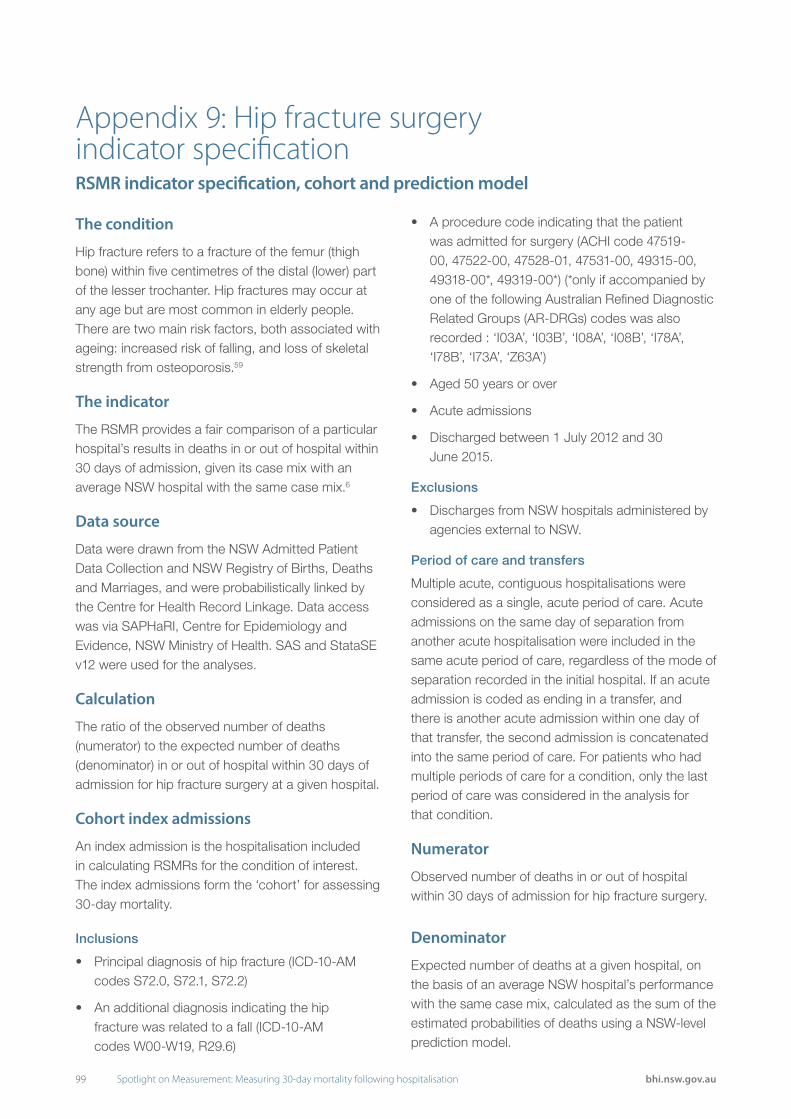
99 Spotlight on Measurement: Measuring 30-day mortality following hospitalisation bhi.nsw.gov.au
Appendix 9: Hip fracture surgery indicator specificationRSMR indicator specification, cohort and prediction model
The condition
Hip fracture refers to a fracture of the femur (thigh bone) within five centimetres of the distal (lower) part of the lesser trochanter. Hip fractures may occur at any age but are most common in elderly people. There are two main risk factors, both associated with ageing: increased risk of falling, and loss of skeletal strength from osteoporosis.59
The indicator
The RSMR provides a fair comparison of a particular hospital’s results in deaths in or out of hospital within 30 days of admission, given its case mix with an average NSW hospital with the same case mix.6
Data source
Data were drawn from the NSW Admitted Patient Data Collection and NSW Registry of Births, Deaths and Marriages, and were probabilistically linked by the Centre for Health Record Linkage. Data access was via SAPHaRI, Centre for Epidemiology and Evidence, NSW Ministry of Health. SAS and StataSE v12 were used for the analyses.
Calculation
The ratio of the observed number of deaths (numerator) to the expected number of deaths (denominator) in or out of hospital within 30 days of admission for hip fracture surgery at a given hospital.
Cohort index admissions
An index admission is the hospitalisation included in calculating RSMRs for the condition of interest. The index admissions form the ‘cohort’ for assessing 30-day mortality.
Inclusions
• Principal diagnosis of hip fracture (ICD-10-AM codes S72.0, S72.1, S72.2)
• An additional diagnosis indicating the hip fracture was related to a fall (ICD-10-AM codes W00-W19, R29.6)
• A procedure code indicating that the patient was admitted for surgery (ACHI code 47519-00, 47522-00, 47528-01, 47531-00, 49315-00, 49318-00*, 49319-00*) (*only if accompanied by one of the following Australian Refined Diagnostic Related Groups (AR-DRGs) codes was also recorded : ‘I03A’, ‘I03B’, ‘I08A’, ‘I08B’, ‘I78A’, ‘I78B’, ‘I73A’, ‘Z63A’)
• Aged 50 years or over
• Acute admissions
• Discharged between 1 July 2012 and 30 June 2015.
Exclusions
• Discharges from NSW hospitals administered by agencies external to NSW.
Period of care and transfers
Multiple acute, contiguous hospitalisations were considered as a single, acute period of care. Acute admissions on the same day of separation from another acute hospitalisation were included in the same acute period of care, regardless of the mode of separation recorded in the initial hospital. If an acute admission is coded as ending in a transfer, and there is another acute admission within one day of that transfer, the second admission is concatenated into the same period of care. For patients who had multiple periods of care for a condition, only the last period of care was considered in the analysis for that condition.
Numerator
Observed number of deaths in or out of hospital within 30 days of admission for hip fracture surgery.
Denominator
Expected number of deaths at a given hospital, on the basis of an average NSW hospital’s performance with the same case mix, calculated as the sum of the estimated probabilities of deaths using a NSW-level prediction model.

100Spotlight on Measurement: Measuring 30-day mortality following hospitalisation bhi.nsw.gov.au
Attribution of index admissions and deaths
In cases of patient transfers, index admissions and deaths are attributed to the first admitting hospital within the period of care.
Development and validation of the prediction model
The NSW-level prediction model was developed using index admissions between 1 July 2009 and 30 June 2012 and using random intercept logistic regression models, taking into account patient-level risk factors (age, sex and comorbidities) and clustering within hospitals.54 A backward modelling approach was used to build the multivariable regression model. Variables significant at the 0.20 level in the univariable analysis were considered for inclusion in the multivariable model. Only variables with a 2-sided p-value of less than 0.05 in the multivariable model were retained in the final model.
The prediction ability of the model was assessed using c-statistics in data from other financial years. The stability of the coefficients in other financial years was also tested. The clinical relevance of the variables in the final model and their direction of association with the outcome were reviewed by clinicians.
The model coefficients were recalibrated using index admissions between 1 July 2012 and 30 June 2015 to calculate the expected mortality for each hospital during that period.
Risk adjustment variables
The following variables are included in the development of the prediction models:
• Age at index admission
• Sex
• The Australian Commission on Safety and Quality in Health Care comorbidity list,57 with a one-year look back period in hospital data.
The final set of risk-adjustment variables for hip fracture surgery were: age, sex, ischaemic heart disease, dysrhythmia, respiratory infection, renal failure, heart failure, malignancy and dementia.
Presentation
Results are presented in a funnel plot. Hospitals with an RSMR that falls beyond the 95% and 99.8% control limits are flagged. Control limits are calculated based on a Poisson distribution.35

101 Spotlight on Measurement: Measuring 30-day mortality following hospitalisation bhi.nsw.gov.au
Figure A9.1 Hip fracture surgery prediction model for deaths in or out of hospital within 30 days, July 2009 – June 2012
Figure A9.2 Hip fracture surgery model performance (c-statistics) over different time periods
Figure A9.3 Hip fracture surgery model coefficient stability, four time periods, July 2003 – June 2015
Predictors Odds Ratio P-value (95% confidence interval)
Age (per year increase) 1.06 <0.001 (1.05 – 1.07)
Female 0.57 <0.001 (0.49 - 0.65)
Ischaemic heart disease 2.19 <0.001 (1.84 - 2.59)
Dysrhythmia 1.35 <0.001 (1.16 - 1.57)
Respiratory infection 1.35 0.001 (1.14 - 1.59)
Renal failure 1.69 <0.001 (1.44 – 1.98)
Heart Failure 1.89 <0.001 (1.59 - 2.25)
Malignancy 1.94 <0.001 (1.47 - 2.54)
Dementia 2.52 <0.001 (2.20 - 2.88)
Period c-statistic
July 2012 – June 2015 0.77
July 2009 – June 2012 0.77
July 2006 – June 2009 0.78
July 2003 – June 2006 0.78
-1.0
-0.5
0.0
0.5
1.0
1.5
2.0
2.5
Coe
ffici
ent
July 2003-June 2006 July 2006-June 2009 July 2009-June 2012 July 2012-June 2015
Appendix 9: Hip fracture surgery indicator specification continued

102Spotlight on Measurement: Measuring 30-day mortality following hospitalisation bhi.nsw.gov.au
103 Spotlight on Measurement: Measuring 30-day mortality following hospitalisation bhi.nsw.gov.au
Appendix 10: Presentation to an emergency department prior to admission
As discussed on pages 27–28, in cases of transfer within an index hospitalisation, patients and their outcomes are attributed to the first admitting hospital. There are cases where a patient first presented to a hospital’s emergency department (ED) but, instead of being admitted to that hospital, they were transferred to a different hospital and admitted. According to the established attribution rules, these patients are attributed to the admitting hospital. The extent to which hospitals are affected by ‘pseudo-transfers’ was explored.
This appendix shows the proportion of index case patients who visited another hospital’s ED in the preceding day for acute myocardial infarction (Figure A10.1) and hip fracture surgery (Figure A10.3). It also presents the crude mortality rates for patients that did and did not visit another ED by hospital for acute myocardial infarction (Figure A10.2) and hip fracture surgery (Figure A10.4).

104Spotlight on Measurement: Measuring 30-day mortality following hospitalisation bhi.nsw.gov.au
Figure A10.1 Proportion of acute myocardial infarction patients who visited another hospital’s ED in the preceding day , July 2012 – June 2015 (Peer group A-C hospitals with at least 50 patients)
Figure A10.2 Acute myocardial infarction, crude mortality by whether patient visited another hospital’s ED in the preceding day, July 2012 – June 2015†
Acute myocardial infarction
NSW (8%)
0 10 20 30 40 50 60 70 80 90 100
% of patients
Lower than expected mortality No different than expected mortality Higher than expected mortalityLower than expected mortality No different than expected mortality Higher than expected mortality
† Peer group A-C hospitals with at least 50 patients overall and at least 5 patients and 5% visit other ED.
* Crude mortality significantly different based on Fisher’s exact test.
Lower than expected mortality No different than expected mortality Higher than expected mortality
Acute myocardial infarction
Hospital 1 5%Hospital 2 5%Hospital 3 9%Hospital 4 5%Hospital 5 20%Hospital 6 8%Hospital 7 10%Hospital 8 8%Hospital 9 22%Hospital 10 14%Hospital 11 19%Hospital 12 7%Hospital 13 34%Hospital 14 9%Hospital 15 20%Hospital 16 23%Hospital 17 17%Hospital 18 10%Hospital 19 18%Hospital 20 14%
Visited other hospital EDfirst %
*
0 5 10 15 20 25 30
Crude mortality rate (per 100)
Did not visit other ED Did visit other ED
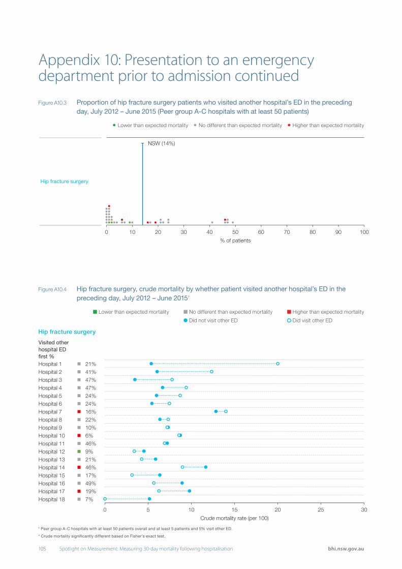
105 Spotlight on Measurement: Measuring 30-day mortality following hospitalisation bhi.nsw.gov.au
Appendix 10: Presentation to an emergency department prior to admission continued
Figure A10.3 Proportion of hip fracture surgery patients who visited another hospital’s ED in the preceding day, July 2012 – June 2015 (Peer group A-C hospitals with at least 50 patients)
Figure A10.4 Hip fracture surgery, crude mortality by whether patient visited another hospital’s ED in the preceding day, July 2012 – June 2015†
Hip fracture surgery
NSW (14%)
0 10 20 30 40 50 60 70 80 90 100
% of patients
Lower than expected mortality No different than expected mortality Higher than expected mortalityLower than expected mortality No different than expected mortality Higher than expected mortality
Hip fracture surgery
† Peer group A-C hospitals with at least 50 patients overall and at least 5 patients and 5% visit other ED.
* Crude mortality significantly different based on Fisher’s exact test.
Lower than expected mortality No different than expected mortality Higher than expected mortality
Did visit other EDDid not visit other ED
Hospital 1 21%Hospital 2 41%Hospital 3 47%Hospital 4 47%Hospital 5 24%Hospital 6 24%Hospital 7 16%Hospital 8 22%Hospital 9 10%Hospital 10 6%Hospital 11 46%Hospital 12 9%Hospital 13 21%Hospital 14 46%Hospital 15 17%Hospital 16 49%Hospital 17 19%Hospital 18 7%
Visited other hospital EDfirst %
0 5 10 15 20 25 30
Crude mortality rate (per 100)
Did not visit other ED Did visit other ED

106Spotlight on Measurement: Measuring 30-day mortality following hospitalisation bhi.nsw.gov.au
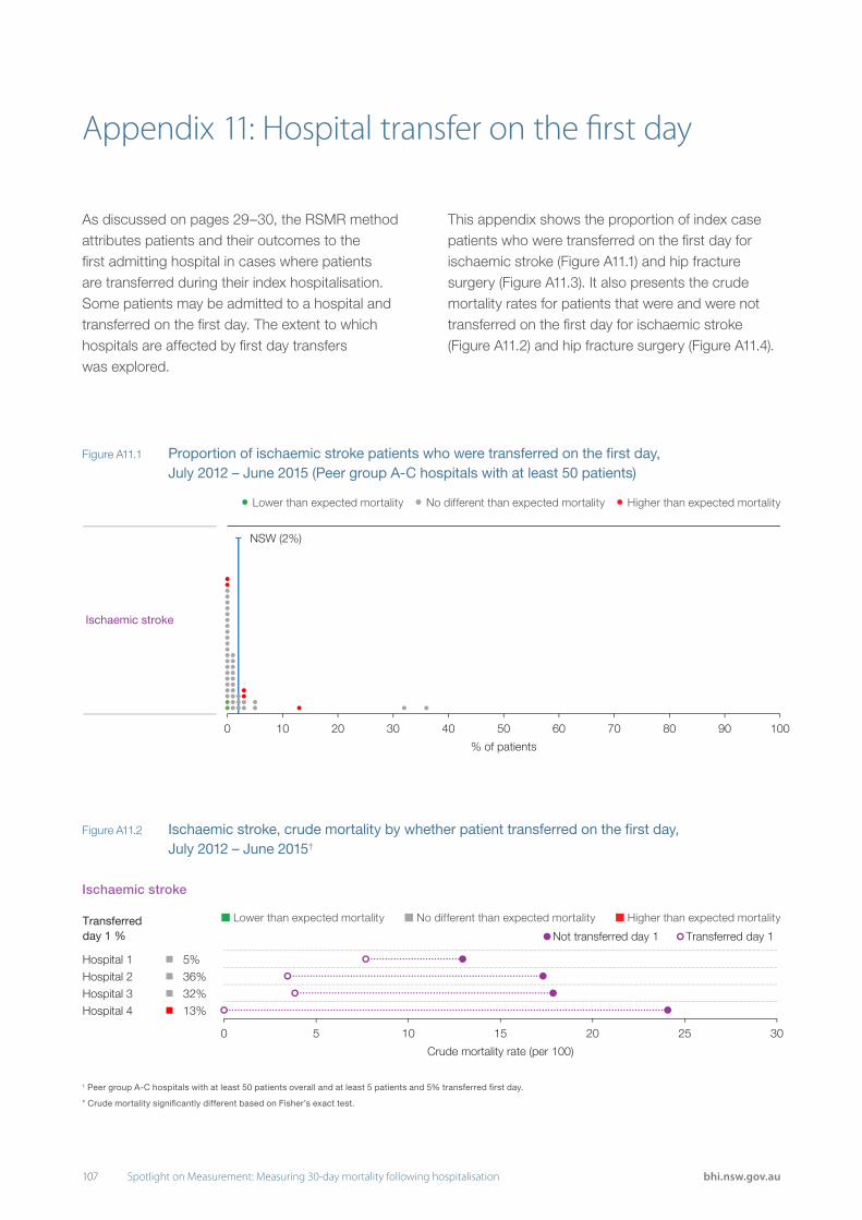
107 Spotlight on Measurement: Measuring 30-day mortality following hospitalisation bhi.nsw.gov.au
Appendix 11: Hospital transfer on the first day
As discussed on pages 29–30, the RSMR method attributes patients and their outcomes to the first admitting hospital in cases where patients are transferred during their index hospitalisation. Some patients may be admitted to a hospital and transferred on the first day. The extent to which hospitals are affected by first day transfers was explored.
This appendix shows the proportion of index case patients who were transferred on the first day for ischaemic stroke (Figure A11.1) and hip fracture surgery (Figure A11.3). It also presents the crude mortality rates for patients that were and were not transferred on the first day for ischaemic stroke (Figure A11.2) and hip fracture surgery (Figure A11.4).
Figure A11.1 Proportion of ischaemic stroke patients who were transferred on the first day, July 2012 – June 2015 (Peer group A-C hospitals with at least 50 patients)
Figure A11.2 Ischaemic stroke, crude mortality by whether patient transferred on the first day, July 2012 – June 2015†
Lower than expected mortality No different than expected mortality Higher than expected mortality
Ischaemic stroke
† Peer group A-C hospitals with at least 50 patients overall and at least 5 patients and 5% transferred first day.
* Crude mortality significantly different based on Fisher’s exact test.
Ischaemic stroke
NSW (2%)
0 10 20 30 40 50 60 70 80 90 100
% of patients
Lower than expected mortality No different than expected mortality Higher than expected mortality
Lower than expected mortality No different than expected mortality Higher than expected mortality
Hospital 1 5%Hospital 2 36%Hospital 3 32%Hospital 4 13%
Transferredday 1 %
0 5 10 15 20 25 30
Crude mortality rate (per 100)
Not transferred day 1 Transferred day 1

108Spotlight on Measurement: Measuring 30-day mortality following hospitalisation bhi.nsw.gov.au
Hip fracture surgery
NSW (4%)
0 10 20 30 40 50 60 70 80 90 100
% of patients
Lower than expected mortality No different than expected mortality Higher than expected mortalityLower than expected mortality No different than expected mortality Higher than expected mortality
Figure A11.3 Proportion of hip fracture surgery patients were transferred on the first day, July 2012 – June 2015 (Peer group A-C hospitals with at least 50 patients)
Figure A11.4 Hip fracture surgery, crude mortality by whether patient transferred on the first day, July 2012 – June 2015†
Hip fracture surgery
† Peer group A-C hospitals with at least 50 patients overall and at least 5 patients and 5% transferred first day.
* Crude mortality significantly different based on Fisher’s exact test.
Lower than expected mortality No different than expected mortality Higher than expected mortality
Hospital 1 22%Hospital 2 14%Hospital 3 25%Hospital 4 8%Hospital 5 9%Hospital 6 16%Hospital 7 5%Hospital 8 23%Hospital 9 11%Hospital 10 13%Hospital 11 21%Hospital 12 7%
Visited other hospital first %
*
*
0 5 10 15 20 25 30
Crude mortality rate (per 100)
Not transferred day 1 Transferred day 1

109 Spotlight on Measurement: Measuring 30-day mortality following hospitalisation bhi.nsw.gov.au
Figure A12.1 Congestive heart failure, percent of acute patients with palliative admission in the year prior by hospital size (Peer group A-C hospitals with at least 50 patients)
0.0
2.0
4.0
6.0
8.0
10.0
12.0
14.0
16.0
18.0
20.0
0 200 400 600 800 1000 1200
Pal
liativ
e ad
mis
sion
yea
r pr
ior
(%)
Number of congestive heart failure patients
No different than expected mortality Lower than expected mortality Higher than expected mortalityLower than expected mortality No different than expected mortality Higher than expected mortality
Appendix 12: Palliative care admissions
This appendix shows the number of acute care patients who had a palliative care admission in the year prior to the index hospitalisation for congestive heart failure (Figure A12.1).
As discussed on pages 31–32, the cohorts for RSMRs are restricted to patients with an acute admission. However, there was some concern that among patients with an acute admission, some may have had a ‘do not resuscitate’ or advance care directive that was not reflected in the hospital administrative record. To investigate this issue a series of descriptive analyses on palliative care were performed.
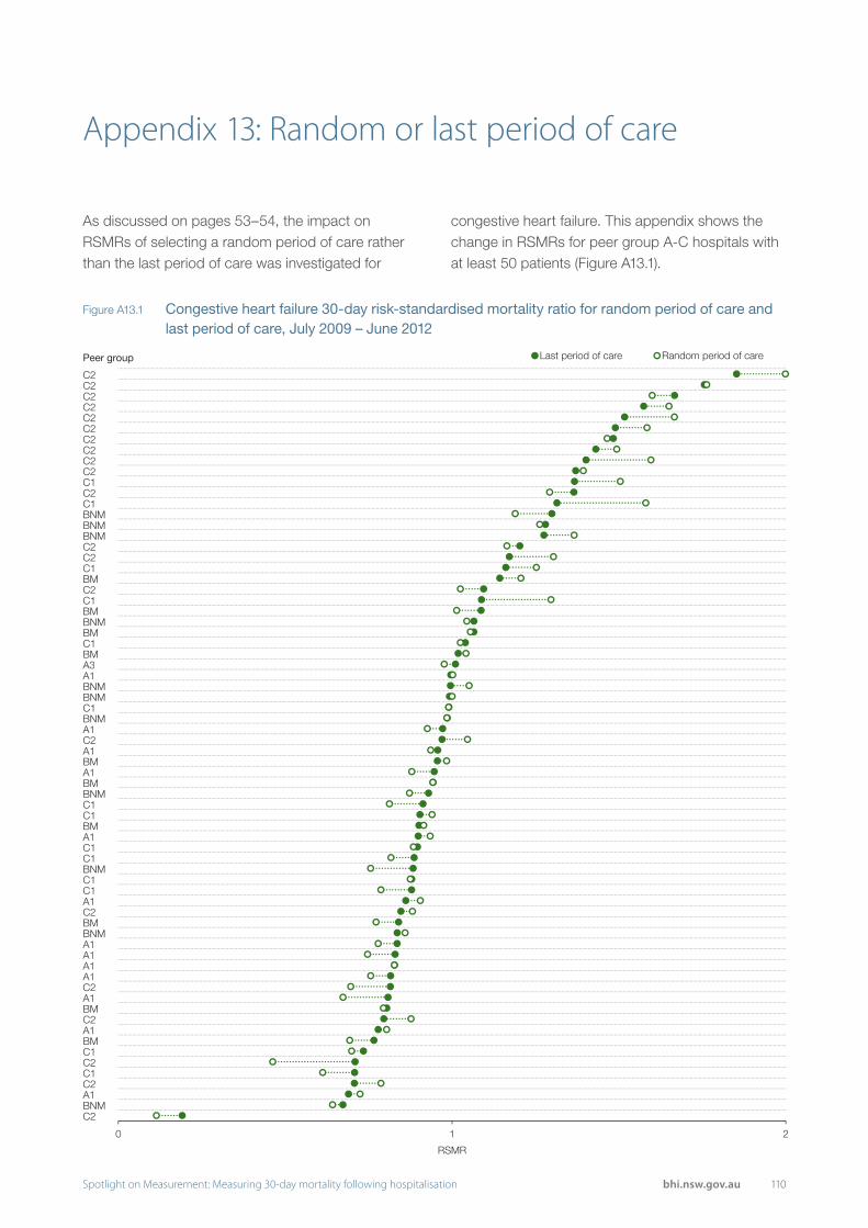
110Spotlight on Measurement: Measuring 30-day mortality following hospitalisation bhi.nsw.gov.au
Appendix 13: Random or last period of care
As discussed on pages 53–54, the impact on RSMRs of selecting a random period of care rather than the last period of care was investigated for
Figure A13.1 Congestive heart failure 30-day risk-standardised mortality ratio for random period of care and last period of care, July 2009 – June 2012
Peer group
C2C2C2C2C2C2C2C2C2C2C1C2C1BNMBNMBNMC2C2C1BMC2C1BMBNMBMC1BMA3A1BNMBNMC1BNMA1C2A1BMA1BMBNMC1C1BMA1C1C1BNMC1C1A1C2BMBNMA1A1A1A1C2A1BMC2A1BMC1C2C1C2A1BNMC2
0 1 2
RSMR
Last period of care Random period of care
congestive heart failure. This appendix shows the change in RSMRs for peer group A-C hospitals with at least 50 patients (Figure A13.1).

111 Spotlight on Measurement: Measuring 30-day mortality following hospitalisation bhi.nsw.gov.au
References
1. Bureau of Health Information. The Insights Series: 30-day mortality following hospitalisation, five clinical conditions, NSW, July 2009 – June 2012. Sydney: BHI, 2013.
2. Bureau of Health Information. Spotlight on measurement: 30-day mortality following hospitalisation, five clinical conditions, NSW, July 2009 – June 2012. Sydney: BHI, 2013.
3. Bureau of Health Information. Indicator specifications: 30-day mortality following hospitalisation, five clinical conditions, NSW, July 2009 – June 2012. Sydney: BHI, 2013.
4. Bureau of Health Information. The Insights Series: 30-day mortality following hospitalisation, seven clinical conditions, NSW, July 2012 – June 2015. Sydney: BHI, 2017.
5. Bureau of Health Information. Spotlight on Measurement: Measuring 30-day mortality following hospitalisation. Sydney (NSW): BHI, 2015.
6. Yale New Haven Health Services Corporation/Center for Outcomes Research & Evaluation. 2014 Measures Updates and Specifications Report Hospital-Level 30- Day Risk-Standardized Mortality Measures. New Haven: YNHHSC/CORE, 2014.
7. Canadian Institute for Health Information. Hospital Standardized Mortality Ratio (HSMR) Technical Notes. Toronto: CIHI, 2014.
8. Health & Social Care Information Centre. Indicator Specification: Summary Hospital-level Mortality Indicator. Leeds: HSCIC, 2014.
9. Dr Foster Intelligence. Understanding HSMRs, A Toolkit on Hospital Standardised Mortality Ratios. London: Dr Foster Intelligence, 2014.
10. Information Services Division Scotland. Hospital Standardised Mortality Ratios, Quarterly HSMR Release, August 2014. Edinburgh: ISD, 2014.
11. Statistics Netherlands. HSMR 2013: Methodological Report. The Hague: Statistics Netherlands, 2014.
12. Taylor R, Aylin P. Mortality measurement: the case in favour. London: Dr Foster Intelligence, 2014.
13. Pouw ME, Peelen LM, Moons KG, Kalkman CJ, Lingsma HF. Including post-discharge mortality in calculation of hospital standardised mortality ratios: retrospective analysis of hospital episode statistics. BMJ. 2013 Oct 21;347:f5913. doi:10.1136/bmj.f5913.
14. Lilford R, Pronovost P. Using hospital mortality rates to judge hospital performance: a bad idea that just won’t go away. BMJ 2010;340:c2016.
15. Black N. Assessing the quality of hospitals. BMJ 2010;340:c2066.
16. Jarman B, Bottle A, Aylin P, Browne M. Monitoring changes in hospital standardised mortality ratios. BMJ. 2005 Feb 12;330(7487):329. doi:10.1136/ bmj.330.7487.329.
17. Keogh B. Review into the quality of care and treatment provided by 14 hospital trusts in England: overview report. London: NHS, 2013.
18. Scott I, Youlden D, Coory M. Are diagnosis specific outcome indicators based on administrative data useful in assessing quality of hospital care? Qual Saf Health Care 2004 Feb;13(1):32-9. doi:10.1136/ qshc.2002.003996.
19. Garnick DW, DeLong ER, Luft HS. Measuring hospital mortality rates: are 30-day data enough? Ischemic Heart Disease Patient Outcomes Research Team. Health Serv Res 1995 Feb;29(6):679-95.
20. Goodacre S, Campbell M, Carter A. What do hospital mortality rates tell us about quality of care? Emerg Med J 2013 doi:10.1136/emermed-2013-203022.
21. Lilford R, Mohammed MA, Spiegelhalter D, Thomson R. Use and misuse of process and outcome data in managing performance of acute medical care: avoiding institutional stigma. Lancet 2004;363:1147-1154. doi: http://dx.doi.org/10.1016/S0140-6736(04)15901-1.
22. Flowers J, Abbas J, Ferguson B, Jacobson B, Fryers P. Dying to know: how to interpret and investigate hospital mortality measures. Liverpool: Association of Public Health Observatories, 2010.
23. NSW Ministry of Health. Admitted Patient Data Collection, Reliabilty and Quality 2015 [online] [cited March 17 2015]. Available from: http://internal.health.nsw. gov.au/data/collections/admitted/reliability.html.

112Spotlight on Measurement: Measuring 30-day mortality following hospitalisation bhi.nsw.gov.au
24. Robertson J, Pearson SA, Attia JR. How well do NSW hospital data identify cases of heart failure? Med J Aust 2014 Jan 20;200(1):25.
25. Marsden DL, Spratt NJ, Walker R, Barker D, Attia J, Pollack M et al. Trends in stroke attack rates and case fatality in the Hunter region, Australia 1996- 2008. Cerebrovasc Dis 2010;30(5):500-7. doi: 10.1159/000319022. Spotlight on Measurement: Measuring 30-day mortality following hospitalisation bhi.nsw.gov.au 56
26. Wang Y, Levi CR, Attia JR, D’Este CA, Spratt N, Fisher J. Seasonal variation in stroke in the Hunter region, Australia. A five-year hospital-based study, 1995-2000. Stroke 2003 May;34(5):1144-50
27. Centre for Health Record Linkage. Quality Assurance 2015 [online] [cited March 17 2015]. Available from: http://www.cherel.org.au/quality-assurance.
28. National Stroke Foundation. Clinical Guidelines for Stroke Management. Melbourne: NSF, 2010.
29. Cadilhac DA, Pearce DC, Levi CR, Donnan GA. Improvements in the quality of care and health outcomes with new stroke care units following implementation of a clinician-led, health system redesign programme in New South Wales, Australia. Qual Saf Health Care 2008 Oct;17(5):329-33. doi: 10.1136/qshc.2007.024604.
30. Heuschmann PU, Kolominsky-Rabas PL, Misselwitz B, Hermanek P, Leffmann C, Janzen RWC et al. Predictors of In-Hospital Mortality and Attributable Risks of Death After Ischemic Stroke: The German Stroke Registers Study Group. Arch Intern Med 2004;164(16):1761-1768. doi:10.1001/archinte.164.16.1761.
31. Fonarow GC, Pan W, Saver JL, Smith EE, Reeves MJ, Broderick JP et al. Comparison of 30-day mortality models for profiling hospital performance in acute ischemic stroke with vs without adjustment for stroke severity. JAMA 2012;308:257–264. doi:10.1001/ jama.2012.7870.
32. Keyhani S, Cheng E, Arling G, Li X, Myers L, Ofner S et al. Does the inclusion of stroke severity in a 30- day mortality model change standardized mortality rates at Veterans Affairs hospitals? Circ Cardiovasc
Qual Outcomes. 2012 Jul 1;5(4):508-13. doi: 10.1161/ CIRCOUTCOMES.111.962936.
33. Bureau of Health Information. Spotlight on Measurement: Return to acute care following hospitalisation, Spotlight on Readmissions. Sydney: BHI, 2015.
34. Schaller B. Ischemic preconditioning as induction of ischemic tolerance after transient ischemic attacks in human brain: its clinical relevance. Neurosci Lett. 2005;377:296–211.
35. Spiegelhalter DJ. Funnel plots for comparing institutional performance. Statistics in Medicine 2005; 24:1185-1202. doi:10.1002/sim.1970.
36. Ben-Tovim D, Woodman R, Harrison JE, Pointer S, Hakendorf P, Henley G. Measuring and reporting mortality in hospital patients. Canberra: AIHW, 2009.
37. Marceau A, Samson JM, Laflamme N, Rinfret S. Short and long-term mortality after STEMI versus non-STEMI: a systematic review and meta-analysis. J Am Coll Cardiol 2013;61. doi:10.1016/S0735-1097(13)60097-2.
38. Krumholz, HM, Lin Z, Keenan PS, Chen J, Ross JS,Drye EE et al. Relationship between hospital readmission and mortality rates for patients hospitalised with myocardialinfarction, heart failure or pneumonia. JAMA 2013; 309:587-593.
39. Vest JR, Gamm LD, Oxford BA, Gonzalez MI, Slawson KM.Determinants of preventable readmissions in the United States: a systematic review. Implement Sci. 2010;5:88.
40. Joynt KE, Jha AK. Thirty-day readmissions – truth and consequences. New England Journal of Medicine 2012;366:1366-1368.
41. Centers for Medicare & Medicaid Services. Medicare Hospital Quality Chartbook, Performance Report on Outcome Measures. Baltimore: CMS, 2014.
42. Health & Social Care Information Centre. Analysis of the Impact of Deprivation on the Summary Hospital-level Mortality Indicator. Leeds: HSCIC, 2014.
43. Harriss LR, Ajani AE, Hunt D, Shaw J, Chambers B, Dewey H et al. Accuracy of national mortality codes in identifying adjudicated cardiovascular deaths. Aust N Z J Public Health. 2011 Oct;35(5):466-76. doi: 10.1111/j.1753- 6405.2011.00739.x.

113 Spotlight on Measurement: Measuring 30-day mortality following hospitalisation bhi.nsw.gov.au
44. Australian Bureau of Statistics. Cause of Death, Australia, 2012 [online] [cited December 22 2014]. Available from: http://www.abs.gov.au/AUSSTATS/[email protected]/allprimarym ainfeatures/2AEDDE570E3A6539CA257E18000F9291?o pendocument.
45. Bureau of Health Information. Public Reporting Improves Healthcare. Sydney: BHI, 2010.
46. Fung CH, Lim YW, Mattke S, Damberg C, Shekelle PG. Systematic review: the evidence that publishing patient care performance data improves quality of care. Ann Intern Med 2008 Jan 15;148(2):111-23.
47. Australian Bureau of Statistics. ABS Data Quality Framework [online] [cited June 10 2015]. Available from: http://www.abs.gov.au/AUSSTATS/[email protected]/ Lookup/1520.0Main%20Features1May+2009.
48. Schulman J, Spiegelhalter DJ, Parry G. How to interpret your dot: decoding the message of clinical performance indicators. J Perinatol 2008;28(9):588-96. doi: 10.1038/jp.2008.67.
49. Seaton SE, Manktelow BN. The probability of being identified as an outlier with commonly used funnel plot control limits for the standardised mortality ratio. BMC Med Res Methodol 2012;16;12:98. doi: 10.1186/1471-2288-12-98.
50. Manktelow, BN, Seaton SE, Evans TA. Funnel plot control limits to identify poorly performing healthcare providers when there is uncertainty in the value of the benchmark. Stat Methods Med Res 2016;25(6):2670-2684.
51. Seaton SE, Barker L, Lingsma HF, Steyerberg EW, Manktelow BN. What is the probability of detecting poorly performing hospitals using funnel plots? BMJ Qual Saf 2013;22(10):870-6. doi: 10.1136/bmjqs-2012-001689.
52. DeLong ER, Peterson ED, DeLong DM, Muhlbaier LH, Hackett S, Mark DB. Comparing risk-adjustment methods for provider profiling. Stat Med 1997;15;16(23):2645-64.
53. Alexandrescu R, Bottle A, Jarman B, Aylin P. Classifying hospitals as mortality outliers: logistic versus hierarchical logistic models. J Med Syst 2014;38(5):29. doi: 10.1007/s10916-014-0029-x.
54. Jones HE, Spiegelhalter DJ. The identification of “unusual” health-care providers from a hierarchical model. The American Statistician 2011;65(3):154-163.
55. Jones HE, Spiegelhalter DJ. Accounting for regression-to-the-mean in tests for recent changes in institutional performance: analysis and power. Stat Med 2009;30;28(12):1645-67. doi: 10.1002/sim.3583.
56. Mohammed MA, Manktelow BN, Hofer TP. Comparison of four methods for deriving hospital standardised mortality ratios from a single hierarchical logistic regression model. Stat Methods Med Res 2016;25(2):706-15. doi: 10.1177/0962280212465165
57. Australian Commission on Safety and Quality in Health Care. National core, hospital-based outcome indicator specification. Consultation Draft. Sydney, ACSQHC, 2012.
58. Elixhauser A, Steiner C, Harris DR, Coffey RM: Comorbidity measures for use with administrative data. Med Care 1998, 36:8-27.
59. Gillespie W (2001) Hip fracture BMJ. 2001 April 21; 322(7292): 968–975.

114Spotlight on Measurement: Measuring 30-day mortality following hospitalisation bhi.nsw.gov.au
C-statistic – A measure of how well a statistical model predicts patient outcomes. The C-statistic ranges from 0.5 to 1.0, with values higher than 0.7 indicating a reasonable model and values higher than 0.8 a strong model.
Fisher’s exact test – A statistical test of independence between two categorical variables used when the sample size is small
Funnel plots – A method of identifying hospitals with outcomes significantly higher or lower than expected that takes into account hospital size and its impact on outcome variability.
Hierarchical logistic regression – A method of modelling patient outcomes that accounts for clustering of patient in hospitals.
Linked data – Data that contains unique patient identifiers, assigned probabilistically on the basis of demographic information such as name, date of birth, gender and address in individual records.
Outliers – Hospitals with significantly higher or lower than expected mortality.
P-value – The probablity of observing a particular result (or something more extreme) if the null hypothesis is true. Generally a p-value of less than 0.05 is considered to provide strong evidence against the null hypothesis.
Period of care – The set of contiguous episodes of acute care, including hospital transfers.
Risk adjustment – The process of using statistical methods to adjust hospital outcome rates for differences in patient risk profiles.
Risk-standardised mortality ratio (RSMR) – The ratio of observed deaths to expected deaths, given the hospitals case-mix.
Rolling time periods – A series of time periods that overlap, for example, a series of two year time periods with one year overlap.
Glossary

115 Spotlight on Measurement: Measuring 30-day mortality following hospitalisation bhi.nsw.gov.au
Acknowledgements
The Bureau of Health Information (BHI) is the main source of information for the people of NSW about the performance of their healthcare system. A NSW board-governed organisation, BHI is led by Chairperson Professor Carol Pollock and Chief Executive Jean-Frédéric Lévesque MD, PhD.
BHI would like to thank our expert advisors, colleagues at the Ministry of Health, reviewers and staff who contributed to the report.
External Advisors and Reviewers
Dr Isuru Ranasinghe Adelaide University
Professor Harlan Krumholz Yale University (CORE)
Dr Terry Symonds Sector Performance Quality & Rural Health, Department of Health & Human Services, Victoria
A/Professor John Worthington Agency for Clinical Innovation, Ingham Institute UNSW, Liverpool Hospital
Dr Peter Kennedy Clinical Excellence Commission
National Health Performance Authority Mortality Directorate
NSW Ministry of Health Health Systems Information & Performance Reporting Centre for Epidemiology and Evidence
Bureau of Health Information Project Team
Research Analysis
Kim Sutherland Huei-Yang (Tom) Chen
Jean-Frédéric Lévesque Julia Chessman (Lead author)
Bradley Drayton
Sadaf Marashi-Pour (Lead analyst)
Design Communications and Stakeholder Engagement
Ed Bury Rohan Lindeman
Adam Myatt Stephanie Watson
Efren Sampaga
Mark Williams


117 Spotlight on Measurement: Measuring 30-day mortality following hospitalisation bhi.nsw.gov.au
About the Bureau of Health Information
The Bureau of Health Information (BHI) is a board-governed organisation that provides independent information about the performance of the NSW public healthcare system.
BHI was established in 2009 to provide system-wide support through transparent reporting.
BHI supports the accountability of the healthcare system by providing regular and detailed information to the community, government and healthcare professionals. This in turn supports quality improvement by highlighting how well the healthcare system is functioning and where there are opportunities to improve.
BHI manages the NSW Patient Survey Program, gathering information from patients about their experiences in public hospitals and other healthcare facilities.
BHI publishes a range of reports and tools that provide relevant, accurate and impartial information about how the health system is measuring up in terms of:
• Accessibility – healthcare when and where needed
• Appropriateness – the right healthcare, the right way
• Effectiveness – making a difference for patients
• Efficiency – value for money
• Equity – health for all, healthcare that’s fair
• Sustainability – caring for the future.
BHI’s work relies on the efforts of a wide range of healthcare, data and policy experts. All of our assessment efforts leverage the work of hospital coders, analysts, technicians and healthcare providers who gather, codify and report data. Our public reporting of performance information is enabled and enhanced by the infrastructure, expertise and stewardship provided by colleagues from NSW Health and its pillar organisations.
bhi.nsw.gov.au