measuring aberrations in lithographic projection systems
TRANSCRIPT
Rochester Institute of TechnologyRIT Scholar Works
Theses Thesis/Dissertation Collections
12-1-2010
Measuring aberrations in lithographic projectionsystems with phase wheel targetsLena Zavyalova
Follow this and additional works at: http://scholarworks.rit.edu/theses
This Dissertation is brought to you for free and open access by the Thesis/Dissertation Collections at RIT Scholar Works. It has been accepted forinclusion in Theses by an authorized administrator of RIT Scholar Works. For more information, please contact [email protected].
Recommended CitationZavyalova, Lena, "Measuring aberrations in lithographic projection systems with phase wheel targets" (2010). Thesis. RochesterInstitute of Technology. Accessed from
MEASURING ABERRATIONS IN
LITHOGRAPHIC PROJECTION SYSTEMS
WITH PHASE WHEEL TARGETS
by
Lena Zavyalova
A dissertation submitted in partial fulfillment of the
requirements for the degree of Doctor of Philosophy
in the Chester F. Carlson Center for Imaging Science
of the College of Science
Rochester Institute of Technology
December 2010
Signature of the Author ________________________________________________________ Accepted by __________________________________________________________________ Coordinator, Ph.D. Degree Program Date
ii
CHESTER F. CARLSON CENTER FOR IMAGING SCIENCE COLLEGE OF SCIENCE
ROCHESTER INSTITUTE OF TECHNOLOGY ROCHESTER, NEW YORK
CERTIFICATE OF APPROVAL
PHD DEGREE DISSERTATION
The Ph.D. Degree Dissertation of Lena Zavyalova
has been examined and approved by the dissertation
committee as satisfactory for the dissertation
requirement for the Ph.D. degree in Imaging Science
_______________________________________ Dr. Bruce W. Smith, Dissertation Advisor _______________________________________ Dr. Maria Helguera _______________________________________ Dr. Karl D. Hirschman _______________________________________ Dr. Joseph G. Voelkel _______________________________________ Date

iii
DISSERTATION RELEASE PERMISSION ROCHESTER INSTITUTE OF TECHNOLOGY
COLLEGE OF SCIENCE CHESTER F. CARLSON CENTER FOR IMAGING SCIENCE
Title of Dissertation
MEASURING ABERRATIONS IN
LITHOGRAPHIC PROJECTION SYSTEMS
WITH PHASE WHEEL TARGETS
I, Lena Zavyalova, hereby grant permission to the Wallace Library of R.I.T. to reproduce my dissertation in whole or in part. Any reproduction will not be for commercial use or profit.
Signature _____________________________ Date _________________________________
iv
MEASURING ABERRATIONS IN
LITHOGRAPHIC PROJECTION SYSTEMS
WITH PHASE WHEEL TARGETS
by Lena Zavyalova
Submitted to the Chester F. Carlson Center for Imaging Science of the College of Science in partial fulfillment of the requirements for the Doctor of Philosophy Degree at
the Rochester Institute of Technology
Abstract
A significant factor in the degradation of nanolithographic image fidelity is optical
wavefront aberration. Aerial image sensitivity to aberrations is currently much greater
than in earlier lithographic technologies, a consequence of increased resolution
requirements. Optical wavefront tolerances are dictated by the dimensional tolerances of
features printed, which require lens designs with a high degree of aberration correction.
In order to increase lithographic resolution, lens numerical aperture (NA) must continue
to increase and imaging wavelength must decrease. Not only do aberration magnitudes
scale inversely with wavelength, but high-order aberrations increase at a rate
proportional to NA2 or greater, as do aberrations across the image field. Achieving
lithographic-quality diffraction limited performance from an optical system, where the
v
relatively low image contrast is further reduced by aberrations, requires the development
of highly accurate in situ aberration measurement.
In this work, phase wheel targets are used to generate an optical image, which can then
be used to both describe and monitor aberrations in lithographic projection systems. The
use of lithographic images is critical in this approach, since it ensures that optical system
measurements are obtained during the system’s standard operation. A mathematical
framework is developed that translates image errors into the Zernike polynomial
representation, commonly used in the description of optical aberrations. The wavefront
is decomposed into a set of orthogonal basis functions, and coefficients for the set are
estimated from image-based measurements. A solution is deduced from multiple image
measurements by using a combination of different image sets. Correlations between
aberrations and phase wheel image characteristics are modeled based on physical
simulation and statistical analysis. The approach uses a well-developed rigorous
simulation tool to model significant aspects of lithography processes to assess how
aberrations affect the final image. The aberration impact on resulting image shapes is
then examined and approximations identified so the aberration computation can be
made into a fast compact model form.
Wavefront reconstruction examples are presented together with corresponding numerical
results. The detailed analysis is given along with empirical measurements and a
discussion of measurement capabilities. Finally, the impact of systematic errors in
exposure tool parameters is measureable from empirical data and can be removed in the
calibration stage of wavefront analysis.
vi
Contents
List of Figures ..................................................................................................................... ix
Symbols and Abbreviations ............................................................................................... xvi
1. Introduction ............................................................................................................... 1
1.1 Overview of lithography systems .............................................................................. 1
1.2 On the lens quality .................................................................................................... 6
1.3 Need for aberration metrology .................................................................................. 7
2. Analysis of aberration measurement methods ......................................................... 10
2.1 The state of the art ................................................................................................. 10
2.1.1 Shearing interferometry .................................................................................. 12
2.1.2 Phase shifting point diffraction interferometry .............................................. 14
2.1.3 Foucault knife-edge and wire tests ................................................................. 16
2.1.4 Phase modulation methods ............................................................................. 17
2.1.5 Ronchi tests .................................................................................................... 18
2.1.6 PSF-based methods ........................................................................................ 22
2.1.7 Aerial image based methods ........................................................................... 24
2.1.8 Wavefront estimation from lithographic images ............................................. 28
2.1.9 Screen tests ..................................................................................................... 35
2.1.10 Summary of methods ...................................................................................... 38
2.2 Scope of this work ................................................................................................... 40
3. Theory of aberrations .............................................................................................. 42
3.1 Pupil description ..................................................................................................... 42
3.2 Zernike description of wavefront aberrations .......................................................... 47
3.2.1 Zernike polynomials ........................................................................................ 48
3.2.2 Rotation through parity states ....................................................................... 56
vii
3.2.3 Orthogonality property ................................................................................... 59
3.2.4 Image quality criteria with aberrations .......................................................... 60
4. Phase wheel aberration monitor .............................................................................. 64
4.1 Overview ................................................................................................................. 64
4.1.1 Image evaluation ............................................................................................. 65
4.1.2 Linear system description – the incoherent and coherent limits .................... 67
4.1.3 Nonlinear system description – the effect of partial coherence on imaging .... 73
4.1.4 Imaging of a phase edge .................................................................................. 76
4.1.5 Imaging a phase wheel target ......................................................................... 85
4.1.6 Influence of even and odd aberration types on phase wheel ........................... 87
4.2 Concept ................................................................................................................... 91
4.2.1 Image formation of phase wheel target with aberrations ............................... 91
4.2.2 Parameterization of phase wheel image .......................................................... 96
4.2.3 Synthetic phase wheel images ......................................................................... 98
4.2.4 Wafer phase wheel images ............................................................................ 100
4.3 Analysis of experimental wafer image data .......................................................... 101
4.3.1 Image processing aspects .............................................................................. 101
4.3.2 Focus-dose analysis ....................................................................................... 112
4.4 Summary ............................................................................................................... 118
5. Phase wheel experimental testing ......................................................................... 120
5.1 Approach ............................................................................................................... 120
5.1.1 Aberration test implementation ................................................................... 120
5.1.2 Mask design .................................................................................................. 122
5.1.3 Target selection and print test ..................................................................... 128
5.2 Phase wheel experimental results .......................................................................... 133
5.2.1 Obtaining wavefront from aerial images of phase targets ............................ 133
5.2.2 Obtaining wavefront from resist images of phase targets ............................. 143
5.2.3 Summary ....................................................................................................... 145
6. Models and experimental implementation ............................................................ 147
6.1 Comparison of parametric and physical models ................................................... 147

viii
6.2 Model generation ................................................................................................... 149
6.2.1 Desired regression models ............................................................................. 151
6.2.2 Design generation ......................................................................................... 153
6.2.3 Model selection ............................................................................................. 156
6.2.4 Model analysis .............................................................................................. 158
6.2.5 Model calibration .......................................................................................... 163
6.3 Optimization problem for aberration retrieval...................................................... 171
6.4 Solution flow overview .......................................................................................... 175
6.5 Model verification using physical data .................................................................. 178
6.5.1 Speed ............................................................................................................. 178
6.5.2 Predictive power ........................................................................................... 179
6.6 Summary ............................................................................................................... 182
7. Implementation results .......................................................................................... 184
7.1 The system representation .................................................................................... 184
7.1.1 Data generation ............................................................................................ 184
7.1.2 Physical and statistical models ..................................................................... 185
7.2 Main results ........................................................................................................... 186
7.2.1 Multiple targets, 13 Zernikes ........................................................................ 187
7.2.2 Quality of fit versus aberration order ........................................................... 192
7.2.3 Single target, 33 Zernikes ............................................................................. 194
7.3 Implementation results summary .......................................................................... 196
7.4 Discussion .............................................................................................................. 198
8. Conclusions ............................................................................................................ 200
References ......................................................................................................................... 204
ix
List of Figures
Number Page
Figure 1.1. Depiction of a projection principle used for pattern transfer in lithography. Light illuminating the mask object (reticle), which defines the chip circuitry, is focused by the reduction objective lens to expose the photosensitive polymer film (photoresist) on the wafer substrate, creating a relief image of the mask pattern in photoresist. Mask (object) and wafer (image) planes typically are the only practically accessible areas inside the system; hence, characterization of projection lens is limited to information gathered at these points of access. ............................................................................ 3
Figure 1.2. Example of a lithography projection lens design for 193 nm wavelength with numerical aperture of 0.8. Inclusion of several aspheric surfaces accomplishes precise wavefront control at each point within the large 8×26 mm image field. Track length of this objective is approximately 1 meter. (Schuster & Epple, 2006) .............................................................................. 5
Figure 3.1. Geometry of the optical imaging: object plane, image plane and pupil planes of an optical system. Note the imaging model must include an illumination source and a condenser lens forming the illumination system. ........... 44
Figure 3.2. Definition of wave aberration function in pupil for a general system. Deviation of ray from a paraxial image point, 1P* , in the image plane is a result of wavefront with aberration,W . The optical path difference, OPD QQ= , is measured along the ray 1QP from the actual wavefront to the reference sphere centered on the ideal image point. ......................................... 46
Figure 3.3. Zernike polynomials for 10n £ , 5m £ . Piston aberration term ( 1; 0)i n m= = = is excluded. At order 9, there are 36 polynomials. ................ 53
Figure 3.4. Zernike polynomials up to the 9th order. Radial degree, n, is mapped vertically; frequency, m, is mapped horizontally. (Scanning left to right from top to bottom, the terms appear in a manner of Malacara & DeVore (1992), Table 13.2, p. 465.) ................................................................................................. 55
Figure 3.5. An example of two possible types of definite parity for aberration function: 13Z is a function with odd radial symmetry
3 313( , ) 8 8 6W x y x y xy xy= + - and 12Z is a function with even symmetry

x
4 4 2 212( , ) 4 4 3 3W x y y x y x= - - + . Here 4n = ; 2m = ; ( ) 2 3n m+ = ,
or 1 5n m+ - = (i.e., fifth order aberration). ...................................................... 57
Figure 4.1. Intensity point spread functions ( )( )2, ; 0h x y z = of a system with
circular aperture associated with a single aberration, for trefoil, astigmatism, and coma. ................................................................................................................ 69
Figure 4.2. Relations that hold between the various 1st order optical functions used for describing the linear optical systems. If partial coherence of illumination must be taken into account, nonlinear system representations must be considered (§4.1.3). .................................................................................................. 71
Figure 4.3. Coherent 1D imaging of a phase edge described in Fourier steps: (a) for ideal diffraction-limited optical system (P is purely real, M is purely imaginary, U is real); (b) for system with coma aberration 7Z (P is complex, U is complex). ......................................................................................................... 79
Figure 4.4. Phase edge with aberrations: (a) pupil phase function for the case depicted in Figure 4.3b; (b) comparison of edge diffraction image intensities obtained from the coherent image amplitudes obtained in Figure 4.3. The aberrated edge centroid is shifted relative to the ideal position, according to PSF of a coma. ........................................................................................................ 80
Figure 4.5. The photoresist image of a 3-bar transparent phase object in the presence of aberrations: (a) an X-oriented test object and its image (cross-sectional profile) in photoresist; (b) a Y-oriented object and its image in resist; (c) test object oriented at 45 degrees and its image in resist. Object transmission is 1; phase difference is from 0 to p. .................................................. 83
Figure 4.6. Phase test target with square shaped p-phase regions and its power spectra versus the object dimensions 1L , 2L , and 3L . ....................................... 84
Figure 4.7. Layout of a test target with multiple p-phase regions. Wheel aberration target with 0°–180°, 90°–270°, 45°–225°, and 135°–315° azimuthal orientations. Chromeless p phase shift design, i.e. the test target is a phase object where we have variations in phase but not in amplitude. ............................ 86
Figure 4.8. Effects of 3rd order astigmatism x and y ( 5Z , 6Z ) on wheel aberration target through focus. Images at 157 nm, 0.85NA, 0.30s in resist. Target dimensions 1 100L = nm, 2 150L = nm, 3 200L = nm. ........................................ 88
Figure 4.9. Effects of primary spherical aberration ( 9Z ) on wheel aberration target through focus. Images at 157 nm, 0.85NA, 0.30s �in resist. Test target dimensions are 1 100L = nm, 2 150L = nm, 3 200L = nm. .................................. 89
Figure 4.10. Effects of coma ( 7Z , 8Z ) and trefoil ( 10Z , 11Z ) on wheel aberration target. Images at 157 nm, 0.85NA, 0.30s �in resist. Target dimensions
1 100L = nm, 2 150L = nm, 3 200L = nm. ........................................................... 91
Figure 4.11. Aberration-free point spread function, ( ) 2h r , for a circular aperture. ..... 94
xi
Figure 4.12. Comparison of diffraction patterns for different aberrations: Zernike polynomial in pupil (top row), the associated coherent PSF magnitude (middle row) and intensity at wafer (bottom row) with axis units l/NA. ............. 95
Figure 4.13. Plots of parametrically defined contours for various coefficients 0r , mc , and ms . .................................................................................................................... 97
Figure 4.14. Phase wheels images simulated in PROLITH. Ideal aberration-free image (a) vs. aberrated image (b). .......................................................................... 99
Figure 4.15. (a) High resolution micrograph of the phase wheel target wafer image obtained with scanning electron microscopy; (b) enlarged image area examined in closer detail. ...................................................................................... 100
Figure 4.16. Ring detection in the phase wheel SEM image with different algorithms: (a) original grayscale image; (b) segmentation result obtained by Canny edge detection; (c) binary image obtained by thresholding, white is the pixel areas above the threshold, and black is below the threshold; (d) segmentation result obtained using the thresholding method - green is inner edge, red is outer edge; (e) final image with outer boundaries and respective centroids superimposed; (f) a magnified view of (e). ............................................. 103
Figure 4.17. Edge detection on a noisy SEM image: (a) input image, (b) horizontal signal profile showing a non-flat background; (c) Canny on raw image, picking up unimportant fluctuations; (d) Canny on image after smoothing and edge linking. Start/end pixel of each segment is marked with asterisk symbol highlighting disjoint boundaries; (e) binary image after thresholding; (f) after morphological processing, with connected components labelled (color coded). ................................................................................................................... 106
Figure 4.18. Using Hough transform for circle detection: a) original image with circles detected; b) composite mask of different regions, based on the detected circle information, setting up for further segmentation with the active contour algorithm. ................................................................................................. 108
Figure 4.19. Segmentation result with active contour algorithm. Active contour evolution of a center ring object in the course of 50 iterations. ............................ 109
Figure 4.20. Result of segmenting the original image in Figure 4.17 using active contour method after 100 iterations. ..................................................................... 110
Figure 4.21. (a) Raw edge (green) vs. parameterized smoothed (red) contours. (b) From pixels to physical dimensions – the spatial scale is given to processed contours. ................................................................................................ 111
Figure 4.22. Image analysis of a phase wheel SEM image (left), and one of the corresponding Bossung plots (right) for response surface model calibration (see §6.2.5). ............................................................................................................ 112
xii
Figure 4.23. Single-target focus-exposure matrix example. Focus step is 0.03 μm, dose step is 1 mJ/cm2. ........................................................................................... 114
Figure 4.24. Example SEM image of a phase wheel test target used for focus-dose analysis in Figures 4.25 and 4.26. Both inner and outer radii of a center ring are modeled using the Focus and Dose variables. ................................................. 115
Figure 4.25. Comparison of the measured (points) and fitted (lines) ring outer radii through dose and focus. The fit R2=0.98, RMSE=0.48 nm. ............................. 116
Figure 4.26. Comparison of the measured (points) and fitted (lines) ring inner radii through dose and focus. The fit R2=0.97, RMSE=0.63 nm. ................................ 117
Figure 5.1. Typical phase wheel target on a two-level 0-p phase shift mask (a) and its image that results on the photoresist coated wafer (b). ................................... 123
Figure 5.2. Target zones and dimensions: 1L , 2L , 3L . ................................................. 124
Figure 5.3. 193 nm reticle layout with 13×17 array covering full scanner field, which is 26×33 mm in dimension at wafer level (104×132 mm at mask level). The module is repeated 13 times in the X-direction of the 26 mm slit, with 2 mm X-spacing between the modules, to get 13 measurable points across the scanner slit. The module is repeated 17 times in the scan direction (Y) for averaging. .............................................................................................................. 125
Figure 5.4. a) Module layout contains a set of 80 different phase wheel targets. Duty ratio and target dimensions are varied. b) Close-up of a test structure and a recognition marker for automated image capture. ...................................... 126
Figure 5.5. 193 nm phase wheel mask layout dimensions table and naming scheme, corresponding to module in Figure 5.4. R3C8 phase wheel identifier label means that dot diameters were 1 2 190L L= = and 3 285L = nm, and opening ( )2 1 2 2 3 2 4L L L L+ + + in chrome shield was 1615 nm. ..................... 127
Figure 5.6. Example of a 193 nm phase wheel mask inspection data. Average mask CD bias is –5 nm; phase depth control is within ±2 deg. ..................................... 128
Figure 5.7. a) The phase wheel object’s phase function (spatial domain), designed with discrete phase values of 0 and 180 deg. b) Fourier transform of the phase wheel function (frequency domain). ............................................................ 129
Figure 5.8. Experimental rings print test. Phase wheel target designs are for a 193 nm 0.85NA system testing. ............................................................................. 132
Figure 5.9. Multiple targets example at best dose. The 1 : 2 : 3 : 4L L L L ratio is varied. .................................................................................................................... 133
Figure 5.10. Phase wheel target aerial image perturbation through focus. The f2 is the nominal (best focus) imaging plane; the f1 and f3 are the defocused planes at +0.15 and –0.15 μm, respectively. .................................................................. 135
xiii
Figure 5.11. Simulated performance: pupil wavefront maps of the actual wavefront (top), the generated solution (bottom left), and the residual surface (bottom right). Fit is based on the 2D aerial images of the phase wheel target acquired at three different focal planes. ........................................... 136
Figure 5.12. Etimated vs. actual aberration coefficient values. ...................................... 137
Figure 5.13. Difference between actual and estimated wavefront coefficient values. ...... 138
Figure 5.14. Standard error on fitted aberration coefficient estimates. .......................... 139
Figure 5.15. In this example, we check the validity of truncating the fit, which could lead to interaction between orders. The wavefront solution is given when expansion is truncated at index i=25. Higher order coefficients ( 26a —
36a ) while present were excluded from the fit. Charted by subgroup (about the individual columns in Fig. 3.3), m=0 represents spherical aberration terms (4, 9, 16, and 25), m=1 comatic x terms (7, 14, 23, and 34), m=2 astigmatic, and so on. The effect of high orders aberration is noticeable at low orders. The solution is generally unsatisfactory and higher order coefficients must be included in the fit.................................................................. 142
Figure 5.16. Phase wheel target image data and fits for 0.90NA 157 nm lens, through focus. Target dimensions 1 200L = nm, 2 250L = nm, 3 200L =nm (2:2.5:2). .......................................................................................................... 144
Figure 5.17. Lens wavefront data: (a) retrieved phase map – RMS OPD 0.040l, PV 0.244l, Strehl 0.927; (b) fitted Zernike coefficients vs. PMI test result. .............. 145
Table 6.1. Table of desired effects and interactions. ....................................................... 152
Figure 6.2. A 5×8 full factorial (left) and a Box-Behnken (right) experimental designs laid out in the coded factor space. Factor values are normalized for the corner points taking values –1 and 1. ............................................................. 154
Figure 6.3. Response surface 4s as a function of 11Z and Dose (left); and 11Z and Focus (right). Response 4s here describes the inner contour of a center ring in a target. 11Z is a trefoil aberration coefficient. All effects values are coded values. ......................................................................................................... 159
Figure 6.4. Response model analysis example for the ring parameter, 4s . Main terms are 11Z and cross-products of 11Z with D, D2, and F2, which account for 98.3% of the total (corrected for mean) variation in the data. ....................... 160
Figure 6.5. Response surface as a function of 5Z , Focus (left) and 12Z , Focus (right). Parameter describes the center ring’s outer contour. 5Z and
12Z are 3rd and 5th order astigmatism x, respectively. Data points are surface plus residuals. ........................................................................................................ 162
Figure 6.6. Response surface as a function of 8Z , Focus (left) and 8Z , 15Z (right). Parameter represents a y-shift in center of gravity of the center
1c
1c
0y
0y
xiv
ring’s outer contour. 8Z and 15Z are 3rd and 5th order coma y coefficients, respectively. Data points are surface plus residuals. ............................................ 162
Figure 6.7. Top row: response surface plots for several particularly F,D-sensitive parameters belonging to various rings. Middle and bottom rows: surface and contour plots (with other factors at their middle setting) resulting of the fitted second-order equation relating response 0r to variables F and D, for 2 different rings. ....................................................................................................... 164
Figure 6.8. Single-target focus-exposure matrix example. Focus step is 0.03 μm, dose step is 1 mJ/cm2. Measured inner and outer radii (responses) of center ring are utilized in the F/D calibration. ............................................................... 166
Figure 6.9. Example of plot option to observe nonlinear fitting process for data in example in Figure 6.8. Raw data (top right) and calibrated data result (bottom right). Raw data fit is R2=0.98, RMSE=0.4543 nm. Calibration model (top left) and fitted (calibration) model equation (bottom left). ............... 168
Figure 6.10. Examples of model response surfaces viewed in three dimensions vs. calibrated focus (μm) and dose correctable, along with measured data (points) used in model calibration: (a) 2s ; (b) 0r ; and (c) 2c parameters for various rings. The dots are experimentally obtained points, which are in close agreement with the computed model of data (surface). (Note that these data also depend on aberrations that will need to be solved for.) ........................ 170
Figure 6.11. Flow chart of wavefront estimation method, including flows for model building and experimental data collection. ........................................................... 176
Figure 6.12. Convergence of model solution during search iterations: 13 vs. 33 Z-term model. The extended model is more computationally costly (to build) but performs an order of magnitude closer reconstruction of the input function than the short model. .............................................................................. 179
Figure 6.13. Measured wavefronts based on experimental phase wheel resist image data from a 193 nm production scanner. Wavefronts for two different lens states are shown, with 5Z aberration physically adjusted. 5Z has been corrected as evidenced in the difference surface, which results in a characteristic astigmatism shape. .......................................................................... 181
Figure 7.1. Absolute deviation in retrieved Zernike coefficients with a 13-term Zernike prediction model built on four test phase wheel targets. The synthetic datasets were built using 13 Zernike terms. The average error in coefficient estimates is 0.0006l. The horizontal axis is the Zernike polynomial index according to fringe Zernike convention. The vertical axis is the magnitude of that aberration coefficient. ........................................................ 188
Figure 7.2. MC analysis error estimate using a 13 Zernike term five-target model, fitting synthetic dataset based on wavefronts with randomly generated 33 Zernike coefficients. Average deviation from true to fitted Zernike values

xv
across all terms is 0.0025 waves. The error is averaged across all 5 MC datasets. ................................................................................................................. 189
Figure 7.3. MC trial fitting result example for one individual sample dataset. Top row is fitted vs. original wavefront. Second row is residual difference surface and retrieved Zernike coefficients. ......................................................................... 191
Figure 7.4. Graphical comparison of synthetic dataset based on actual wavefront vs. the fitted wavefront produced by 2 different models. The two models presented were built using 13 and 22 Zernike terms, while synthetic dataset was based on full 33 terms in Zernike expansion. A single target was used. (Single target fit to 13 and 22 Zernike-term models. The 13-term model predicts 4Z — 16Z coefficients, while the 22-term model operates on 4Z —
25Z coefficients. Fringe Zernike numbering scheme is used.) ............................. 193
Figure 7.5. Wavefront error estimate using a 33 Zernike term single-target model, fitting synthetic dataset based on wavefronts with randomly generated 33 Zernike coefficients. Average deviation from true to fitted Zernike values across all terms is 0.00159 waves .......................................................................... 195

xvi
Symbols and Abbreviations
Symbol Equation
ia ith Zernike polynomial coefficient; also Zi (3.2)
a Zernike coefficient vector (3.2), (6.8)
a reconstruction vector (6.9)
a optimization parameter(s) in model (6.4)
( )xG illumination cross-spectral density (4.13)
( )xg illumination degree of coherence (or coherence function) (4.12)
nnd ¢ Kronecker delta (3.12)
( )xd Dirac delta (4.19)
( )1 2,x x bilinear transfer function (4.13)
l wavelength of radiation, [nm] (1.1)
0x spatial frequency (4.1)
maxx spatial frequency limit (4.16)
( ),x h spatial frequency coordinates in a pupil plane, see §3.1
( )o ⋅ cost function (6.4)
xvii
r normalized radial pupil coordinate vector, see §1.2
( ),r q angular coordinates in a pupil plane, see §3.1
s degree of partial coherence in a projection exposure system
2Ws variance of aberration function ( ),W r q (3.18)
( ),r qF phase function; also ( )xF (3.1), (4.17)
( )xY PTF (4.3)
0y phase shift (4.2)
0 0 0
0 0
, , ,
,
a b c
d f
é ùê úê úê úë û
calibration model parameters, see §6.2.5
ijc coefficient in CD FE model, see §4.3.2
D exposure dose, [mJ/cm2] (4.25)
E irradiance, [W/m2]
F defocus position, [nm] (4.25)
( )F x object transmission spectrum (4.14)
f measurement matrix (6.9)
f reconstruction matrix (6.9)
( )f a image matrix; also f (6.8)
( );f x b general response surface model (6.1)
( )f x input signal (4.4)
xviii
( )g x output signal (4.4)
( ),H x h OTF; also ( )H x (4.3), (4.10)
( )H x MTF (4.3)
( )h x coherent impulse response; also ( ),h x y , or ( ),h r q (4.6)
( ) 2h x incoherent impulse response (4.8)
I aerial image intensity (4.1)
k wavenumber (3.1)
( )1 2,k x x double impulse response (4.12)
1k lithography process factor for minimum feature size (1.1)
( )L ⋅ sum of cost functions (6.4)
1, 2, 3L L L phase wheel target dimensions, see §5.1.2
M number of images (6.8)
( )M x mask object spectrum (4.16)
m intensity image modulation (4.2)
( )m x mask object transmission (4.16)
NA numerical aperture at image side (1.1)
( )⋅ order of neglected terms, see §4.2.1
( ),r qP complex exit pupil function; also ( ),x hP (3.1)
xix
( ),lnR r q radial part of ( ),l
nV r q (3.3)
( )mnR r radial part of Zernike polynomial (3.6)
S Strehl ratio (3.19)
U image electric field (4.15)
mnU real Zernike polynomial (3.4)
( ),lnV r q complex Zernike polynomial (3.3)
( ),W r q wavefront aberration function for circular pupil; also ( )W r
, or
( ),W x h , [nm] or [l] (3.2)
w minimum half-pitch, [nm] (1.1)
( ), ,x y z geometrical coordinates of an optical system, see §3.1
0 0
0
, ,
, ,m m
x y
r c s
ì üï ïï ïí ýï ïï ïî þ ring contour shape parameters (4.21)
Zi factor name for ith Zernike polynomial coefficient (same as ia ), see §6.2.1
( ){ }iZ r
a set of Zernike basis functions, see §1.2
( ),iZ r q ith Zernike polynomial; also iZ (3.2)
Mathematical Notation Equation
auto-correlation (4.10)
Ä convolution (4.5)
2⋅ Euclidean norm (6.9)

xx
{ }⋅ Fourier transform
{ }1- ⋅ inverse Fourier transform
nÎa logical evaluation if a is an element of n (6.9)
n n-space (6.9)
Abbreviation
ART aberration ring test
CCD charge-coupled device
CD critical dimension, [nm]
CTF contrast transfer function
DPP discharge produced plasma
DUV deep ultraviolet region of the radiation spectrum (100–300 nm wavelength)
ENZ extended Nijboer-Zernike theory
EUV extreme ultraviolet region of the radiation spectrum (10–20 nm wavelength)
FEM focus-exposure matrix
IC integrated circuit
IFT inverse Fourier transform
ILIAS integrated lens interferometer at scanner
ITRS International Technology Roadmap for Semiconductors
xxi
LPP laser produced plasma
LSI lateral shearing interferometry
MC Monte Carlo
MTF modulation transfer function
NA numerical aperture
OPD optical path difference, [waves]
OTF optical transfer function
PMI phase measuring interferometry (or phase stepping interferometry)
PSF point spread function
PSPDI phase shifting point diffraction interferometry
PTF phase transfer function
RMS OPD wavefront departure from sphericity, defined as root-mean-square value of
phase over the pupil, [waves]
RMSE root-mean-square error
SEM scanning electron microscope
TAMIS transmission image sensor at multiple illumination settings
TCC transmission cross-coefficient
TIS transmission image sensor
UV ultraviolet region of the radiation spectrum (10–400 nm wavelength)

1
1. Introduction
1.1 Overview of lithography systems
The performance of semiconductor devices has improved significantly since the integrated
circuit (IC) was invented in 1958. The pace of this development is governed by "Moore’s
Law". In 1965, Gordon E. Moore, co-founder of Intel Corporation, estimated that the
number of transistors integrated in a chip approximately doubles every two years. This
prediction was merely an extrapolation of observed early trends, which has maintained for
over four decades. With the transistor count on today’s microprocessor chips approaching 2
billion (Intel.com, 2010), the chip density, power and speed have all seen similar exponential
growths. Chip silicon area size, however, has remained relatively unchanged. The increase
in feature density and performance advancements are primarily due to downscaling
dimensions of active chip components. The key technology that enables the scaling of circuit
pattern sizes is nanolithography.
Lithography imaging employs projection printing techniques for pattern transfer, where a
circuit design from a photomask is transferred into a radiation sensitive material
(photoresist) atop a silicon wafer, by exposure with deep ultraviolet (DUV) radiation. This
typically involves a very high resolution lens operating at a single DUV wavelength
2
generated with a line narrowed excimer laser source. Only one level of a pattern can be
transferred with one mask, resulting in multiple lithographic levels being needed to make a
full chip.
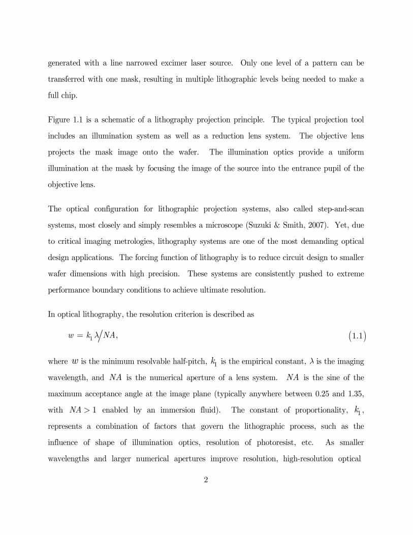
Figure 1.1 is a schematic of a lithography projection principle. The typical projection tool
includes an illumination system as well as a reduction lens system. The objective lens
projects the mask image onto the wafer. The illumination optics provide a uniform
illumination at the mask by focusing the image of the source into the entrance pupil of the
objective lens.
The optical configuration for lithographic projection systems, also called step-and-scan
systems, most closely and simply resembles a microscope (Suzuki & Smith, 2007). Yet, due
to critical imaging metrologies, lithography systems are one of the most demanding optical
design applications. The forcing function of lithography is to reduce circuit design to smaller
wafer dimensions with high precision. These systems are consistently pushed to extreme
performance boundary conditions to achieve ultimate resolution.
In optical lithography, the resolution criterion is described as
where w is the minimum resolvable half-pitch, 1k is the empirical constant, l is the imaging
wavelength, and NA is the numerical aperture of a lens system. NA is the sine of the
maximum acceptance angle at the image plane (typically anywhere between 0.25 and 1.35,
with 1NA > enabled by an immersion fluid). The constant of proportionality, 1k ,
represents a combination of factors that govern the lithographic process, such as the
influence of shape of illumination optics, resolution of photoresist, etc. As smaller
wavelengths and larger numerical apertures improve resolution, high-resolution optical
1 ,w k NAl= ( )1.1
3
Figure 1.1. Depiction of a projection principle used for pattern transfer in
lithography. Light illuminating the mask object (reticle), which defines the chip
circuitry, is focused by the reduction objective lens to expose the photosensitive
polymer film (photoresist) on the wafer substrate, creating a relief image of the mask
pattern in photoresist. Mask (object) and wafer (image) planes typically are the only
practically accessible areas inside the system; hence, characterization of projection
lens is limited to information gathered at these points of access.
lithography has been developed towards very short wavelengths and very high NA . The
operating wavelength has decreased from 436 nm (Hg g-line source) to 193 nm (high energy
ArF excimer laser source), and is currently making a transition to 13.5 nm, for which
extreme ultraviolet (EUV) sources are needed that generate enough x-ray photons to meet
Substrate scan
Wafer image
Projection lens, NA
Mask objectZ
Reticle scan
Light source, l
Condenser optics
4
throughput requirements. This evolution is found in the roadmap for silicon-based
semiconductor technology that defines technological milestones (nodes) of the
miniaturization trend for the next decade (ITRS, 2009). Accordingly, the roadmap for
semiconductor lithography addresses the expectation of lithographic processes—development
times and trends—versus the nodes and indicates the challenges that need to be overcome in
moving to a new technology. Projection lens quality plays an important role at each node.
As the geometries of semiconductor devices continue to shrink below the wavelength used for
imaging, significant demands are being placed on the quality of projection optics. Projection
systems capable of sub-wavelength resolution must comprise a large number of optical
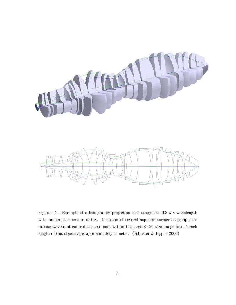
elements. In this regard, Figure 1.1 is an extreme simplification. Figure 1.2 illustrates the
complexity of an optical system that must use many lenses and several aspherical surfaces
when large fields and high apertures are involved. The design in the figure is representative
of lithography lenses with a numerical aperture of 0.8 at 193 nm. The height of the system
shown is 1000 mm, the image field is 8×26 mm and the wavefront aberrations are corrected
down to a root-mean-square (RMS) error of five thousandths of a wavelength (5 ml ).
High-accuracy lithography projection systems require that aberration effects are fully
characterized. Systems must be optimized to achieve a high degree of aberration correction.
Every surface error, due to fabrication, encountered in the beam path between the object
and the image will add to the resulting wavefront aberration. The level of residual
aberration in these systems must be minimized to allow resolving powers on the order of
0.30 l/NA. This type of performance is near the physical limit of diffraction and requires an
optical wavefront aberration approaching a l/200-level for state-of-the-art systems. Such
Fig
wit
pre
leng
gure 1.2. Ex
h numerical
cise wavefro
gth of this o
xample of a
l aperture of
ont control a
bjective is ap
lithography
f 0.8. Inclu
at each point
pproximatel
5
projection l
usion of seve
t within the
y 1 meter. (
lens design f
eral aspheric
large 8×26
(Schuster &
for 193 nm w
c surfaces ac
mm image f
Epple, 2006
wavelength
ccomplishes
field. Track
6)
6
aggressive requirements pose extremely high challenges for fabrication of lenses and even
higher challenges for metrology methods needed to characterize them.
To satisfy the extreme specifications on imaging performance, modern projection exposure
tools have evolved to be very complex partially coherent optical imaging systems. Many
challenges are presented concerning rigorous specifications of image formation, complex
simulation tools, and characterization of optical aberrations.
1.2 On the lens quality
Lens quality can be described as the ability of an optical system to convert a spherical
wavefront emerging from an object point into a spherical wavefront converging toward a
geometrical image point in an image plane (Goodman, 1996). Aberrations, as the term
implies, introduce deformations to a propagating spherical wavefront, resulting in image
quality degradation. For example, aberrations reduce image contrast, lead to pattern
distortions, trigger image displacements and shifts of focus. Aberrations can result from
misaligned optical elements, surface imperfections, or be inherent in the optical design.
In order to obtain qualitative measures for discrepancies between actual and ideal images,
image variations are also characterized on the basis of wavefront aberrations. The
degradation in the quality of a wavefront is determined by the amount of phase change it
contains when compared to an unaberrated wave originating from the same object. The
deviations from the ideal wavefront, also called optical path length errors, are expressed in
fractions of the wavelength or in nanometers. They are captured in the aberration function,
( )W r
, which is defined in the pupil plane of the imaging lens. An arbitrary wavefront
( )W r
, where r is a pupil coordinate vector (normalized to the maximum lens NA) is often
expanded in terms of a set of Zernike polynomial functions ( ){ }iZ r
that allow for
7
separation of wavefront error into different aberration types, each with a different physical
effect. Wavefront and aberration definitions will be introduced in Chapter 3.
Aberrations are one of the main sources of image variations in lithography systems. Tight
critical dimension (CD) specifications of circuit features are what dictates allowable levels of
aberration tolerances for a photolithographic application. In a phase-coherent lithographic
imaging process, the relative phase relationships must not be affected by the image-forming
lens. The lithography projection systems must perform at diffraction limits. Conventionally,
an acceptably diffraction-limited lens is one which produces no more than one-quarter-
wavelength optical path length error. While this l/4-rule constitutes the diffraction-limited
performance for many non-lithographic lens systems, the reduced performance resulting from
this level of aberration is not allowable in lithography applications (Flagello & Geh, 1998).
The resolution specification needs of today’s DUV (ArF and KrF) lithography require
balanced aberration levels below l/20 OPD RMS (all aberrations averaged over the lens).
Future requirements dictate unprecedented wavefront accuracies at sub-l/200 performance
(Williamson, 2005). Moreover, with the application of newer imaging techniques that
enhance the resolving power of a lithographic projection system, such as phase-shift masks or
off-axis illumination, lithographic requirements and tolerances are even more stringent. In
those specific imaging situations, performance of the utilized portion of the pupil is as
important as full pupil performance (Smith, 1999).
1.3 Need for aberration metrology
Scaling of critical dimensions into the sub-100 nm level causes many issues that were not
seen as critical before. One of the main issues is the scaling of aberration of lithographic
lenses with NA. According to the ITRS 2009 roadmap, ultra-high NA objectives are
8
required for 193 nm optical lithography, which has a profound impact on aberration
requirements. Aberrations are a serious concern as their effect on image becomes more
pronounced for high NA as it scales with NA powers, NA2, NA3, NA4, NA5, etc. (Williamson,
1994). The roadmap predicts that a much shorter EUV wavelength that represents a jump
to 13.5 nm would be introduced at 22 nm and 16 nm technology nodes. The use of shorter
wavelengths allows a lower NA for the same resolution. As the operating wavelength
reduces, however, residual aberrations increase linearly relative to wavelength. The residual
aberration has to be maintained at a fraction of the wavelength l of the light. It is
estimated that the measurement precision of l/1000 must be available; the measurement
accuracy must reach l/1000 in order to be effective.
Aberration metrology is a critical step in the production process of quality lithographic lenses
and is an area of great practical importance when monitoring lens performance in an IC
fabrication environment. The lithographer needs to understand the influences of aberration
on imaging and any changes that occur in the aberration performance of the lens after its
assembly and its installation on the scanner. Aberrations are not constant and can change
over time. Wavefront aberrations will also change over the course of using an exposure tool.
A further problem is that the imaging quality of high performance optical systems is
susceptible to environmental influences such as temperature, pressure, mechanical loads and
other disturbances, hence monitoring of imaging errors and aberration control is essential
during tool use. Mechanical stability wavefront requirements extend beyond mere design
aberration challenges. For instance, even an extremely small temperature or air pressure
change is sufficient to cause fluctuations in the nanometer to micron range.
In order to minimize and control the aberrations, lithography projection systems have
several movable lens elements (van der Laan & Moers, 2005). The imaging wavelength and

9
the position of a mask table are also adjustable. Reversible changes (e.g., as caused by lens
heating) may temporarily change the aberrations. These changes to the lens also require
small readjustments. When these adjustments are made, different aberrations may be
introduced. Moreover, since the intensity of excimer laser radiation is very high, the
components of a projection system are prone to laser damage so that the aberrations will
change during the lifetime.
Consequently, there is a requirement of being able to measure aberrations reliably and
accurately. Devices and methods for aberration measurement are needed to determine the
imaging errors of high-precision imaging systems. Reliable, sufficiently accurate
measurement methods must be available for this purpose, to allow efficient characterization
of the projection objectives in situ. An in situ aberration measurement technique is,
however, met by a number of challenges, which are to be discussed in Chapter 2.

10
2. Analysis of aberration measurement
methods
2.1 The state of the art
This chapter will focus on the mix of direct and indirect (noninterferometric) methods, their
functional principles, and their capacity to measure large optics in situ. Some discussion is
of historical interest but, otherwise, the review is mainly of methods that can be adapted to
lithographic lens characterizations.
The most significant advancements in development of lithography tools have become the
development of different types of optical testing instrumentation and analysis algorithms to
facilitate actinic (at-wavelength) wavefront measurements. While at-wavelength
implementation is typically more difficult than with visible light, it is critical that the same
wavelength radiation is used.
Modern lithographic lenses are qualified during manufacturing stages with the use of a phase
measuring interferometry (PMI). PMI, which is highly developed, generally entails both
data collection and analysis methods which are used by all major lithographic lens
11
manufacturers today. The method is also known as the phase shifting or phase stepping
interferometry (PSI) and is one of the principal methods of measuring wavefront aberrations
(Greivenkamp & Bruning, 1992). The basic concept behind PMI is that a time-varying
phase shift is introduced between a reference wavefront and a test wavefront. At each
measurement point, a time-varying signal produces an interferogram; and a relative phase
difference between the two wavefronts at each position is encoded within these signals.
Highly accurate measurements possible with phase stepping interferometry are due to the
decreased sensitivity to systematic errors encountered in static interferogram analysis.
While the PMI method remains the gold standard with lens manufacturers, it is primarily
developed for ex situ characterization. The lithographer in the field is still restricted to using
alternative approaches to monitor lens aberration performance.
Most of the subtle experimental conditions are encountered in interferometry. Precision
interferometry methods require a careful control of external vibrations, as vibrations cause
unstable phase shifts. But, a more significant limitation of these interferometric methods is
the need for the reference and test beams to follow separate paths, making in situ application
difficult. In a conventional interferometer used with PMI, such as a Twyman-Green, Fizeau,
or Mach-Zehnder, the test and reference beams must be allowed separate optical paths.
Perfect optics are needed in the reference branch of an amplitude-splitting interferometer or
a wavefront splitting device in a shearing interferometer. Coherence length requirements
have to be satisfied and necessary mechanical and environmental stabilities are difficult to
obtain. These are the main difficulties with employing conventional interferometers for
in situ measurements in a lithography tool.
A common optical path approach is preferable within the confines of a lithography tool. The
common-path section is the portion of the interferometer through which the test beam as

12
well as the reference copy propagate. Common-path design interferometric methods of
measurement will therefore be reviewed in §§2.1.1 and 2.1.2.
Interferometric tests are not the only schemes available for determining wavefront
aberrations. In addition to pure interferometric techniques, several other types of
noninterferometric metrology systems exist or are under development for in situ wavefront
measurements, which could potentially reach the accuracy requirements for lithography
projection optics. Sections 2.1.3 through 2.1.9 will contain a review of various non-
interferometric methods as they apply to measurement of lithographic lenses in situ.
2.1.1 Shearing interferometry
Shearing interferometry is a wavefront measurement technique that makes use of the self-
referencing principle: the wavefront to be tested is interfered with a sheared copy of itself.
The copied wavefront is subjected to a shift, a rotation, or a radial shear, hence its name. A
shear interferogram then gives the interference pattern that describes a phase difference
between the original and sheared wavefronts over the shear distance. When this distance is
small, the wavefront difference function is roughly proportional to a phase gradient of the
wavefront (i.e., the average local slope) in the direction of shear. An orthogonal set of phase
gradient maps is required in order to yield a reconstructed wavefront.
There are a number of methods for producing sheared wavefronts. One adaptation of
shearing interferometer to a lithographic projection system has been developed by ASML.
ILIAS (integrated lens interferometer at scanner) is based on a lateral shearing principle
(van de Kerkhof et al., 2004).
13
The ILIAS interferometer arrangement contains a point source at the object plane (reticle
level) in combination with a shearing diffraction grating at the image plane (wafer level).
The grating splits the aberrated wavefront into multiple laterally sheared copies. The
resulting interference pattern of the sheared wavefronts is formed at the far field. As such,
this ASML scheme can be considered a variation of a Ronchi interferometer that will be
discussed in §2.1.5. Subsequent imaging optics are arranged such that the detector camera
plane (a two-dimensional CCD array) is conjugate with the exit pupil plane of the lens
system being measured. Only the lowest diffraction orders from the grating are considered.
Spurious higher diffraction orders are suppressed using Fourier filtering techniques. The
phase map spatial resolution is roughly NA/25 waves, defined by the shear distance.
Aberration levels in lithographic projection lenses are typically low, and thus only a small
variation of intensity, instead of the typical strong interferometric fringe pattern, is expected.
To increase the accuracy of the phase gradient map, the measurement is performed
dynamically by means of a phase stepping technique. The relative phase-shifting steps of a
signal on a detector are accomplished by translating a grating over equidistant steps.
Precise knowledge of these lateral displacement increments is necessary. A series of
interferograms, each separated by a p/8 phase shift, have to be recorded. The speed of the
measurement is determined by 1) the integration and readout times of the detector; 2) the
number of phase steps and the computation time for determining the phase; and 3) the
subsequent calculation time of the aberration coefficients of the wavefront.
The accuracy reported for an ILIAS interferometer is roughly 2.5 ml at the 193 nm
wavelength. The reported measurement reproducibility is between 0.5 and 2.5 ml (3s),
depending on the aberration type (van de Kerkhof et al., 2004).
14
An advantage of the shearing wavefront measurement principle is its ability to work with
partially coherent light sources. The challenge for shearing interferometers is the precision
requirements on the positioning systems controlling the axial and lateral displacements of a
grating optical component, caused by the drift phenomena or vibration of the entire
measurement structure. Precision of phase-shifting steps is an important factor to achieve
high measurement accuracy. The displacement increments have to be accurate down to a
few nanometers, which can be difficult to achieve without expensive precision mechanical
components in conjunction with highly accurate measurement and drive systems.
Alternatively, as part of the operating method, an additional measurement system for
monitoring of the exact positioning of the phase-shifting steps is needed to reduce the
otherwise possibly very high requirements on translators, regulation and mechanics of an
associated positioning system. These measured values can be acquired for each phase-
shifting step and taken into account as correction values during phase calculations.
2.1.2 Phase shifting point diffraction interferometry
The alternative to lateral shearing interferometry is phase shifting point diffraction
interferometry (PSPDI). A prototype PSPD interferometer has been developed by workers
at Lawrence Berkeley National Laboratory to measure EUV lithography optics at an
operational wavelength of 13.4 nm (Medecki et al., 1996). RIT has utilized a similar method
at UV and DUV wavelengths (Venkataraman & Smith, 2000).
The PSPD interferometer is a common path interferometer that incorporates a pinhole
diffraction to generate wavefronts of high spherical accuracy. This method uses a diffraction
grating to produce angularly sheared test and reference beams. The grating is illuminated
through a pinhole with a spherical wavefront. A zero diffraction order beam is directed
15
through the optic being tested and experiences aberration present within the lens pupil. A
higher grating diffraction order beam is sent through the edge of the lens pupil and is
subsequently spatially filtered by a second pinhole, which is smaller than the diffraction-
limited resolution of the optic, and becomes a spherical reference beam. If the reference
pinhole is perfect, any aberration in this beam is removed. The test beam and the reference
beam are interfered and sampled for various grating steps to reconstruct the pupil wavefront
phase. Data collection during the full field measurement requires approximately 6 hours.
Algorithms used for this approach are similar to those used for PMI techniques.
The advantage of this common path design is a lesser sensitivity to system vibration and
turbulence. Another obvious benefit to this method is the short operational wavelength.
The wavefront measurement accuracy has been reported as 0.06 nm RMS and repeatability
is reported as 6 pm for small NA EUV optics (Naulleau et al., 2001; Goldberg et al., 2002).
The two primary sources of measurement error with this method are systematic effects that
arise from the geometry of the system (which can be compensated, if measurable) and
imperfections in the pinhole. Pinhole imperfections result in reference beam errors,
dependent on size, shape, and positioning of the pinhole. There is a flux limitation that can
pass through a pinhole, hence the imbalance of power between the test and the reference
beams. The above factors create a trade-off between efficiency and accuracy. The third
perceived constraint on accuracy of this method’s design is its susceptibility to speckle noise.
It can be alleviated by introducing a filtering element into configuration and combining
phase stepping and Fourier fringe pattern analysis schemes (Naulleau & Goldberg, 1999).
Although the PSPD interferometric method has potential for accurate wavefront
measurement, implementation will likely be difficult without major modifications to the
stepper or scanner hardware. Since interferograms must be detected beyond the image
16
plane, a system under testing must allow access at these positions. Large numerical
apertures will also make image capture difficult and secondary optical relay systems may be
required. Finally, while the PSPDI approach has been successfully demonstrated with a
synchrotron undulator beamline, the high cost and limited availability of such highly
coherent point sources preclude their use as a lithography production source. Laser
produced plasma (LPP) and discharge produced plasma (DPP) based EUV radiation sources
being developed for use in production will not sustain the same flux density at the necessary
coherence level for PSPDI testing.
2.1.3 Foucault knife-edge and wire tests
Foucault (1859) first introduced a knife-edge test for testing the telescopes, which has since
been modified and widely applied to many optical systems. In the Foucault test, a knife-
edge is inserted in the focal plane, covering one-half of the return beam. The aberrations of
the test object are analyzed by recording the intensity distribution on a conjugate pupil
plane behind the focal plane. If the lens system is free from error and, therefore, able to
focus the rays into a point image, the whole pupil appears uniformly illuminated. Any
deviation of the light rays from their undisturbed path results in a dark shadow formed over
aberrated pupil regions. A variant of this method is also known in literature as a schlieren
imaging technique proposed by Töpler (1864). The name originates from a German word
referring to striae or optical inhomogeneities in glass. The Foucault test is a special case of
the Töpler experiment.
The Foucault test is a sensitive method for detecting small errors in optics, and it is simple
and inexpensive to perform. One advantage is that since the setup is not based on
interference, the requirement for coherent light is far less stringent. The drawbacks are the
17
loss of half the light and non-linearity problems. The main complication limiting the use of
the classical knife-edge test is difficulty in obtaining quantitative results.
As in other methods, when testing surfaces with a fast varying slope, many annular zones
have to be inspected. Thus, the actual accuracy of the method will depend on the number of
zones, diffraction at the edge, precision of the edge movement, and complexity of the surface
profile. Another limitation to Foucault test is that it is insensitive to small wavefront slope
changes in either magnitude or direction, which is the case when the first and second
derivatives of the wavefront errors are small. This is especially problematic with large
apertures (Ghozeil, 1992). Its calibration requires accurate photometry which is more
difficult than the phase measurement of fringe scanning interferometry. The precision is not
as good as that of shear or PSPD interferometry methods.
Another method of testing, known as the wire test, is a modification of Foucault test that
makes it easier to obtain quantitative results. The behavior of the shadow pattern produced
by wire, again, is characteristic of the spherical, defocus, coma, and field curvature
aberration types present in the system. Various enhancements to this approach have proven
capability at the levels needed for microlithography application but implementation may be
difficult. Mechanical knife-edges or a wire must be placed within the optical system with
tight tolerance over placement and parallelism.
2.1.4 Phase modulation methods
An improvement to the Foucault test, where the phase edge removes the need to use a
physical method to block light, was first proposed by Zernike (1934) and is known as a phase
contrast test. The phase contrast test, as well as other related techniques developed since,
essentially perform an optical image processing in Fourier space, e.g. by placing a l/4 phase
18
shifting disk artifact in the optical path in order to obtain linear phase modulation in the
image intensity. The resulting diffraction patterns exhibit a modulation of phase in first
order and can be correlated to the wavefront aberration. Hence, these are a class of pupil
filtering techniques made to make phase function on image intensity linear.
A l/2 phase edge test, due to Wolter (1956), is another variation on the Foucault knife-edge
test. From a geometrical optics point of view, the shadow grams associated with the l/2
phase edge are considered to be identical with the shadow patterns associated with the wire
test. The sensitivity of the l/2 phase edge test is greater than the sensitivity obtained when
using an opaque knife-edge or the wire test.
2.1.5 Ronchi tests
Ronchi method has received ample discussion in the literature and is relatively simple
conceptually. In a traditional Ronchi arrangement, a diffraction grating is positioned near
the optical system focus, which is a point of convergence of the aberrated (test) wavefront,
such that the image of the grating is superimposed onto the grating itself, producing an
interference pattern. The approach has been used in many testing applications since Ronchi
first introduced it in 1923 (Ronchi, 1964).
Ronchi grating interferometry is closely related to a number of tests. For instance, it may be
regarded as a multiple wire test concept. Under certain conditions, the lateral shearing
interferometry (LSI) is equivalent to the Ronchi test, namely if a grating is used to split the
measured wavefront into multiple diffracted orders that overlap each other in the far-field
region forming interference fringes (as discussed in §2.1.1). Interestingly, Ronchi technique
has also been shown to bear some relation to the Hartmann screen test (Cornejo-Rodriquez,
1992).
19
The interference pattern in a ronchigram contains information about the wavefront slope in
a direction perpendicular to the grating structure. Because shearing in only one direction
gives wavefront gradient with respect to only one coordinate, measurements with two
orthogonal grating orientations are needed to reconstruct the wavefront aberration function.
Owing to the grating, Ronchi technique has many practical advantages such as variable
sensitivity and large dynamic operational range, as well as flexible spatial filtering. One
difficulty with using a single Ronchi grating orientation is that slope in only one direction is
obtained. This means that the grids on orthogonal ronchigrams must correspond to the
same coordinate system on the unknown wavefront. A double-channel Ronchi system
design, to acquire the orthogonal slope data simultaneously, is needed. The two channel
systems generally have higher cost and complexity. To get around the two-channel design
and to reconstruct the measured wavefront from a single ronchigram, the use of two-
dimensional version of Ronchi gratings (crossed gratings) has been suggested, but the
interpretation of resulting patterns becomes more difficult.
When applying Ronchi tests to lithographic systems there are additional practical aspects to
be aware of. Firstly, the classical Ronchi test typically uses rather low frequency diffraction
gratings, and fringe analysis can be performed using a simple geometric optical model. For
best results the pitch of the grating is chosen such that no more than two diffraction orders
will overlap at any given point, and the fringes can be interpreted as due to interference of
two beams only. This condition dictates the shear ratio l/(2NA pitch) of 0.5. If a high
resolution optical system with either high NA or a short wavelength l needs to be tested,
the Ronchi test with shear ratio of 0.50 has the disadvantage that pitch of the gratings can
be very small. Particularly in EUV systems operating near 13 nm, the pitch at l/NA tends
20
to be very small with the values well below 70 nm. Due to the small pitch, it is challenging
to fabricate the gratings, and the setup’s vibration sensitivity is high.
Secondly, for the Ronchi test to be used with the highly corrected (highly resolving)
lithography lens systems, the method requires increased sensitivity at small shears, which are
two competing objectives. The reconstruction of a small wavefront aberration from the
measured phase difference (slope) is optimum if the shear ratio is considerably less than one
half of the pupil diameter. This calls for use of seemingly simpler, larger pitch gratings. The
limitation of using low frequency gratings however, are the spurious interference terms from
higher diffraction orders that complicate the quantitative evaluation of ronchigrams. Hence,
in the case of small phase gradients and shears, fringe contrast and accuracy of the results
are severely limited by diffraction and additional spatial-filtering operation is required to
select only two interfering diffraction orders, such as by means of a stop in the focal plane.
Diffraction orders of the Ronchi grating must, therefore, be geometrically accessible to enable
filtering. Spatial filtering in a defocused plane (Schwider, 1981) can be cumbersome in a
Ronchi test with an extended source and restrict the applicability to lithography systems to
some extent.
Several modifications and extensions of Ronchi test have been proposed, directed at
obtaining an arbitrarily small shear for more accurate measurements. The double-frequency
grating (Wyant, 1973), which is simply a grating containing two closely spaced frequencies
made to have only two-beam interference of the first-order waves associated with each
frequency, is not practical for lithography application as it still requires high average spatial
frequency gratings. To avoid the complicated manufacture of high frequency gratings, Braat
and Janssen (1999) proposed a specific grating layout that suppresses unwanted higher-order
interference at low shear ratios and adapted the Ronchi interferogram analysis for an
21
arbitrary source intensity function. Their modified setup was based on the use of a matched
pair of gratings: a Ronchi grating (as a shearing unit) and a source grating (as an extended
periodic light source). Such concept enabled the Ronchi test with an extended source, rather
than a point source, in which the entrance pupil is illuminated in a partially coherent way.
The ability to use extended sources and relaxed coherence requirements have significance for
lithography applications for systems with large field of view and partially coherent
illumination. It is especially attractive for characterization of EUV projection mirror optics
and would allow a larger part of the EUV source to be used, leading to a shorter data-
collection time. However, the absolute accuracy of this interferometer is of the order of
0.01l RMS, as estimated with the visible wavelength light setup (Hegeman et al., 2001).
At-wavelength implementation is typically more difficult than with visible light.
Additionally, since a single beam splitting (shearing) element is employed the Ronchi
interferometer is simple to align and stabilize against mechanical vibrations. It has,
however, some important disadvantages. The shear amount is fixed by the grating
frequency, good contrast fringes are obtained for the lateral shear equal to at least half of the
diameter of the beam under test, and the number and orientation of reference fringes cannot
be arbitrarily chosen. As such, without many special modifications, the method is not
adapted to the measurement of the small residual aberrations of aberration-limited systems.
Practical application for lithographic purposes is therefore limited. The method is easier for
the scanner manufacturer to integrate within a tool at the design stages than it is for the
user to retrofit the tool after the tool has been fully assembled.
22
2.1.6 PSF-based methods
This class of methods performs characterization of optical imaging systems by measuring the
three-dimensional structure of the point spread function (PSF). The principle of these
methods makes use of the fact that the irradiance in a defocused image is not homogeneous
and has unique structure when wavefront has aberrations.
The observation of defocused stellar images, known as the star test, has long been known as
a sensitive method to detect small wavefront aberration. Early application of the technique
dates back to Taylor (1896). It involves examining the image of a point-like object, such as
a star, formed by the lens and determining the departures in the irradiance distribution from
its ideal form. The intensity point-spread functions (Airy patterns), coupled with changes in
and out of focal plane, are unique for each aberration type. These patterns—diameters of
dark rings, distances between axial zeros, etc.—possess noticeable structure that can allow
aberration levels to 0.02–0.05l to be detected by evaluation of encircled energy and image
contours of constant intensity. Historically the star test came to be primarily a qualitative
visual method of evaluating small imperfections in high quality image-forming systems, until
tools and quantitative methods began to develop. This is due to a fact that the aberrated
point spread functions possess very complex structure that is difficult to treat analytically.
Aberration retrieval from the through-focus intensity point spread function in lithography
application has not been attempted until very recently (Dirksen et al., 2003a).
An analytical expression for the point spread function for an out-of-focus region in the
aberration-free case was first obtained by Lommel in 1885 (Born & Wolf, 1997). Zernike
and Nijboer (1942) derived the analytic expression for the PSF in optical diffraction problem
in the presence of small aberrations. More recently the analysis has been revisited by
Janssen (2002), who extended the near-focus diffraction integral to through focus, combining
23
the diffraction theories of Airy, Lommel, and Nijboer. The approach was termed extended
Nijboer-Zernike theory (ENZ). It provides a rigorous analytical description of through-focus
image intensity of the PSF, including effects of aberration. ENZ is of practical interest to
lithographic testing as it allows treatment of problem of aberration retrieval by providing an
analytical solution to the star test analyzing Airy patterns. Starting from intensity data in
the focal volume, viz. the aberrated intensity point spread function of the optical system, it
allows a backward calculation to obtain the complex field in the exit pupil.
The original ENZ diffraction analysis was first limited to the scalar optical fields, valid for
imaging systems with relatively low numerical apertures (smaller than 0.60). The optical
model was later extended to include vector diffraction effects. Refinements to the retrieval
technique were also added to account in the diffraction integral for effects like the use of
pinholes of finite size and the radiometric effect (Braat et al., 2003).
The scalar ENZ test was applied in the optical lithography setting by Dirksen et al. (2003b),
where the projection lens aberrations were derived from recorded point source images in a
photoresist layer. In the experimental procedure, a point source was achieved by means of a
pinhole in the chromium mask layer with a diameter of 0.5 l/NA in the object space. The
measurement is based on observation of the intensity point-spread function pattern in-focus,
as well as defocused patterns on the both sides of best focal plane. For each exposure, the
printed resist image is developed up to a certain contour of equal intensity (slice) in the
point-source image. By varying the exposure dose between successive images in the resist
layer, a whole range of equal intensity contours of the point images is obtained. By
analyzing the contour plot of each resist image, for the complete series of defocused resist
images at varying exposure, one can reconstruct the three-dimensional intensity distribution
in the focal volume.
24
Dirksen et al. (2003b) discussed using resist images in scalar retrieval method at l=193 nm
and NA=0.63. The reported measurement spread in the retrieved coefficients is of the order
of ±10 ml, resulting in RMS wavefront deviation of less than 3 ml. The short term
repeatability is of the order of a few ml.
The ENZ inverse problem test also has been extended to the case of high-NA optical systems
with vector optical fields (Dirksen et al., 2005). As applied to assessment of a lithographic
projection lens with a high NA (l=193 nm, NA=0.85), the accuracy was shown to be of the
order ~1.6 ml for a 40 ml of spherical aberration 9Z . It was noted that the contours
cannot be experimentally obtained at high intensity levels where the contour diameter
becomes small, beyond the recording capability of photoresist. It was also noted that the
point spread function deformation by aberrations is most visible at low intensities where the
diffraction ring structure is found. The contour line broadening that is due to the resist
diffusion and focus blurring in the lateral and axial directions must be accounted for by the
model.
The first results of the high-NA aberration retrieval have been reported to be obtained for
simulated data with high theoretical accuracy. Actual high-NA aberration retrieval may
prove challenging to obtain from photoresist images in practice, since diffraction limited
pinhole images (multiple slices) will be difficult to record with detail in a photoresist layer.
2.1.7 Aerial image based methods
A number of techniques based on direct measurement of the projected aerial image have
been attempted for characterization of optical systems for many applications, by directly
measuring aerial image using an image sensor. The basic concept of direct measurement idea
is that the output response (e.g. image modulation measurements) of a system for a specific
25
input can lead to characterization of error mechanisms (e.g. transfer function). For partially
coherent imaging (such as in lithography imaging), a modulation transfer function treatment
is ambiguous, but approximate linear models exist that model some aspects of the system.
The measured parameter can be one or more of: the position of best-focus of the image; the
lateral displacement of the image; the asymmetry of the image structure. The results of
these image measurements can be characterized by various parameters, for example, a
curvature of the aerial image CD curve through focus. Focus offsets can be determined from
experimental curves of image intensity modulation versus defocus, and so on.
A number of difficulties always arise with the wavefront measuring methods based on aerial
image assessments for optical lithography. First is the problem with the analysis –
separating of aberration types and understanding their contribution to changes in the image.
Small levels of aberration can have similar impact and identification of various (azimuthal)
orders is difficult. The lower-order Zernike coefficients can be determined in this way, and
the accuracy is also limited. The models are for low order aberrations primarily. Higher
orders retrieval from modulation metric is not feasible. Second set of challenges with these
methods comes with making the mask artifacts and the detector that are small enough to
give the resolution required for images of interest, accurately producing arrays of these
features at the detector. Third challenge is getting sufficient energy though a small pinhole
or slit feature onto the detector. Acquiring lithographic aerial images requires a special DUV
detector. The sensors must be designed for use with high NA, in order to avoid reduced
sensitivity resulting in less accurate measurements, before radiation reaches the final
detecting element.
One aerial image-based approach proposed jointly by GCA/Tropel and UC Berkeley (Partlo,
Fields, & Oldham, 1993) is based on correlating aerial image contrast to 4 of the 5 primary
26
Seidel aberrations. They are astigmatism, distortion, field curvature, and spherical
aberration. The effects of spherical aberration, for example, are identified by simulated
contrast vs. defocus curves with using the only 3rd and 5th order spherical aberration terms,
all other terms set at zero. The astigmatism is found by measuring the difference in best
focus between sagittal and tangential line/space features of different pitch, and so on. The
accuracy limit of this method is unknown. A model for analysis of image and contrast
transfer has not been disclosed.
Another example in lithography using aerial image measurement, developed more recently
by ASML (van der Laan et al., 2001), is a technique called TAMIS (transmission image
sensor at multiple illumination settings). The technique is based on aerial image
measurements with the alignment sensor (TIS), a measurement device built into the wafer
stage of step-and-scan system. The two main functions of the TIS are monitoring system
best focus drift during operation and aligning the wafer stage to the reticle stage. To enable
them, the TIS is capable of measuring lateral (x,y) and axial (z) positions of projected
images. Measurements of the best focus (z) or a lateral shift (x and y) are required
depending on whether even or odd aberration must be determined. For example, one effect
of spherical aberration is to shift the position of best focus in the z direction and this is used
to determine coefficients for Zernike poynomials 9Z and 16Z . Matching the measured shifts
to shifts determined by a lithographic simulator, allows extracting individual aberration
components.
A system of this type is designed and works as follows (van der Laan & Moers, 2005). It
consists of 2 gratings and a photodiode for a detector to measure the intensity behind one of
the gratings. The detector makes use of moiré patterns formed between the image of a
projection grating and a complementary detection grating. The image sensor is scanned so
27
that, as the aperture passes through the light and dark portions of the image, the output of
the photodetector will fluctuate, which is used as a measure of the defocusing. If the
projected image is in focus and aligned with the grating on the detector, all radiation passes
through, resulting in the maximum intensity at the detector. If the image is not in focus at
the grating or is misaligned with the grating, the intensity measured by the detector will be
lower.
The method is using aerial image measurement of 1.5 micron dense lines and 0.25 micron
isolated spaces, in which the aerial image sensor scans the best focus positions in the x and z
directions for various field locations and for various exposure settings. The vertical level at
which the rate of change of amplitude of the photodetector output is highest indicates the
level at which the image has the greatest contrast and hence indicates the plane of optimum
focus. The horizontal level at which the rate of change is highest indicates the aerial image’s
lateral position.
The aberration-induced effects will depend on the sampling of the pupil, which can be
modified by imaging different test structures, and by varying the illumination partial
coherence (s) and lens NA. In fact, eight different numerical aperture and illumination
sigma settings are typically required. From these measurements of x, y, z-shifts as a function
of NA/s, the lower order aberrations are calculated.
TAMIS measures the following lowest order Zernikes only: coma x and y ( 7Z , 8Z , 14Z ,
15Z ), spherical ( 9Z , 16Z ), "HV" astigmatism ( 12Z , 21Z ). Higher-order Zernike coefficients
are not included in the model. Accurate determination of low order tilt ( 2Z , 3Z ) and
astigmatism ( 4Z , 5Z ) is not possible, since these absolute measurements require a well-
calibrated reticle and image sensor. Detection excludes the trefoil aberration due to large
dense line grating targets not sensitive to trefoil effect.
28
Linear models are used to solve for Zernike coefficients, where each measurement that
corresponds to the NA and s setting is modeled as the sum of weighted Zernike coefficients.
For example, for coma x, it is a correlation of the lateral shift Dx to 2Z , 7Z and 14Z
coefficients at multiple optical settings. The lithographic sensitivities to each individual
aberration are derived from simulated data by a lithographic simulator one at a time, all
other aberrations being zero. The model is a linear approximation which neglects higher-
order quadratic and cross-terms, and so on, although these could potentially be taken into
account. The applicability of the linear model is determined by simulation (Flagello et al.,
1997).
The precision of the measurement technique is approximately 1 nm (0.005l) for each Zernike
coefficient. The 3s reproducibility is 3 nm. The average difference between this method and
PMI data is reported at 2 nm for spherical and astigmatism. Lithographic wafer test
comparisons demonstrate good matching with model.
Depending on the requirements on accuracy and repeatability, this is a good test that offers
the possibility to accurately measure low order aberrations fast. Because the device is
integrated with the imaging system, it allows to perform the measurements directly and use
them to implement the necessary system corrections and lens adjustments in real time.
Advantages include robustness and speed because it is a direct measurement technique not
involving exposure of a resist.
2.1.8 Wavefront estimation from lithographic images
There has also been significant interest in developing and demonstrating a class of in situ
methods to infer lens aberration through measurement of printed lithography image
structures of particularly sensitive mask features. Through the use of techniques similar to
29
those used with aerial image approaches, aberrations can be estimated from resist images
and focus shifts. These methods of measurement lead to an estimation based on knowledge
of how a particular aberration should influence a particular image.
Lithographer typically has a number of ways of pupil sampling that can be used to probe
particular portions of a wavefront, such as with the use of any resolution enhancement
techniques (phase shift masking and off-axis illumination) where only particular potions of a
pupil are utilized. This fact can be taken advantage of by designing illumination or phase
masking that resonates with particular aberrations. For example, an alternating phase shift
mask structure can be quite sensitive to astigmatism and three-point. The images of such
features can be measured and compared with simulated images using known levels of
aberration. The accuracy of matching an aberrated wavefront using this type of estimation
is increased by including a range of different conditions and by limiting evaluation to those
conditions that would most likely be experienced in a real imaging situation.
(a) The first such technique that has matured to a reasonable commercial level is the phase
shift focus monitor test developed by IBM (Brunner et al., 1994). As it uses lines and spaces
with 90 degree phase (phase structures being sensitive to finding focus), the phase shift focus
monitor approach is useful for fitting lumped low-order aberrations, but discrimination
among the different aberration terms is difficult. Since the method is not fully
comprehensive to each aberration term, complete description of the aberrated wavefront is
infeasible.
(b) Kirk & Progler (1999) have introduced a method to measure wavefront aberration using
a phase grating reticle to direct diffraction orders to particular portions of a lens pupil. The
process by which a grating is made to diffract most of the light in the desired order is called
blazing, and the grating is called blazed. These blazed gratings are oriented at various angles

30
(from 0° to 337.5° at 22.5° increments) for adequate azimuthal coverage. The image of the
grating is micro-stepped through focus and recorded into the photoresist top surface. A
second blanket exposure is made, resulting in a composite developable latent image formed
that is linearly related to the recorded aerial image intensity. The resulting images contain
aberration information for the portion of the lens pupil sampled by the diffraction energy
directed at the blazed angle. By using several grating angles, both low and high angular
frequency aberration terms can be distinguished.
An algorithm has been developed to fit aberrations from measured resist images. As with
many resist-based evaluation methods, the capability of this approach requires matching the
images recorded in resist to simulation with various aberration types. This approach is not
limited to symmetrical aberration types only because gratings can be arranged over a wide
range of orientations (azimuths). The main limitation of this method is the ability to
measure high radial order aberrations. The capability of the blazed grating approach
increases by adding grating pitches (frequencies) on the test reticle. Accuracy of this method
has been reported to be within 12% of RMS OPD of the measured wavefront.
Improvements are possible by using lower values of partial coherence. By lowering partial
coherence, s, approaching coherent illumination condition, the averaging effect imparted on
diffraction orders can be reduced, but current exposure tools have a limit on the lowest s
value. Fabrication of a test grating becomes challenging as a large range of etch angles must
be accommodated. Special photoresist material is also required for this method. Ideally, a
resist should be of low contrast and highly absorbing in a photochemical sense. This implies
that the resists used for IC fabrication would not be well suited and special materials and
modifications to processes would most likely be required.
31
(c) A method of wavefront sampling, using binary line mask structures, is described in
Kaise, Tsukakoshi & Hayashi (2001), where the amount of aberration is determined on the
basis of a difference between line widths. This method is adequate for the detection of
comatic aberrations but it is difficult to extract the magnitude of such aberrations or the
presence of other aberrations.
(d) Yeung (2000) described a pupil exploration method using 1D binary gratings. The
method is based on measurement from printed photoresist patterns of periodic lines of focus
and image displacement for two different pitches and six orientations (0, ±30, ±60, 90).
This amounts to a set of 12 grating objects produced under nearly fully coherent
illumination. Experimental CD versus focus curves are constructed. The model then relates
image intensity distribution to the dimension of the printed photoresist patterns, which can
be written exactly for 3-beam interference under the idealized imaging conditions, i.e. fully
coherent, centered, monochromatic illumination and a grating object with symmetrical
profile and of infinite size. The overall measurement precision of l/50 for the OPD should
be possible with this method and the corresponding individual Zernike terms to an accuracy
of l/50 also.
(e) The imaging of strong (l/2) phase edges is an interesting option for lithography
applications requiring in situ aberration measurements. The main idea is that it is possible
to make differences of energy in the image directly proportional to differences of phase in the
pupil.
One such phase modulation method is called the aberration ring test (ART) developed by
Dirksen et al. (1999; 2000) at Philips Research Laboratories. The ART method uses a test
object, shaped as a single cylindrical phase-dot with diameter ~l/NA and a l/2 phase
depth. The dot appears as a ring in the image plane where ring is defined by a phase edge.
32
The image of this ring is exposed into resist at the particular condition of illumination and
resist is developed. The resulting images are scanned using a scanning electron microscope
(SEM). The scanned images undergo image processing and are subsequently analyzed to
extract lens aberration in the form of lumped aberrations of a specific class that are further
separated into individual Zernike terms assuming that a linear relationship exists between
them. The measurement results represent families or lumped terms, grouped by aberration
type. The Zernike coefficients are solved from a set of linear equations. The model
parameters are determined by means of lithographic simulation. For example, one of the
studied responses is a tilt of isofocal for ring width. It is used to solve for coefficients of
spherical aberration terms 9Z , 16Z , and 25Z . Solution is obtained using multiple optical
conditions NA and s, where the product NA*s is a constant, i.e. source size is constant.
ART method is reported to be capable of determining up to 25 Zernike coefficients with a 3s
reproducibility from 0.006 to 0.020l, depending on the aberration type (Moers et al., 2001).
The accuracy of the ART method is highly dependent on the quality of the linear model
which is used to treat the simulation data. A comparison with the shearing interferometry
measurement method shows that the linear model is suitable but to a limited extent, as the
method becomes less stable the greater the number of orders of Zernike coefficients that are
intended to be separated. Compared to Zernike coefficients obtained from interferometric
measurements, the mean and standard deviation of differences in ART-obtained coefficients
was at 0.005l and 0.007l, respectively. The method requires measurements using multiple
optical conditions, at different NA and partial coherence s, to improve the estimation. This
complicates the experimental procedure to some degree by requiring multiple exposure and
measurement passes. Large amounts of data are often needed for conclusive results. The
method also requires additional step of finding best focus and optimal exposure dose before
metrology data collection and analysis can be undertaken.
33
(f) In another image-based method, Berkeley researchers (Neureuther et al., 2006) developed
special phase shift mask features they named a pattern and probe-based aberration monitor.
Aberrations in a lens system are identified by projecting an optical beam through a mask,
having an opening (a probe) and a surrounding pattern, and through the lens to an image
plane. The pattern is designed to channel its power into the probe peak.
In particular, the mask feature geometries consist of a nominally sub-printable circular probe
with diameter ~0.45 l/NA, surrounded by a ring of chrome, and a series of concentric rings
(pattern), which alternate in phase between 0 and 180 degrees. The probe acts as an
interferometric reference and is phased 90 deg for even aberrations and at 0 deg for odd
aberrations. While probe will not print on its own, the coherent “spillover” of electric field
from the pattern is designed to cause the probe to print, when the aberration is present.
The signals from the probe and the pattern become intermixed, creating a composite pattern
in the image plane with aberrations altering the image intensity (Robins, Adam, &
Neureuther, 2002).
In general, the patterns are complex phase-shifting structures which change both radially
and angularly in phase. The exact radial and angular dependencies of the pattern rings
depend on the specific Zernike aberration term that it is designed to resonate with. Different
aberrations require a separate pattern design. Patterns each have a layout based on the
inverse Fourier transform (IFT) of a given aberration function with the carefully optimized
sizing in targeting sensitivity to a particular aberration level. The inverse Fourier transform
of aberration function is used to only determine the mask pattern that will maximize the
coupling into the image of the central pixel (probe); the effect of this pinhole is independent
of the level of aberrations and is disregarded in studying the additive perturbation due to
aberrations (Robins et al., 2002).
34
The IFT-based procedure implicitly assumes coherent illumination rather than the partial
coherence used in various illumination schemes in projection printing. But it is possible to
simulate the image of this pattern under the partially coherent illumination conditions
utilized in printing the wafer.
One of the main reported benefits of pattern and probe-based aberration monitors is high
selectivity to the aberration they are designed to detect and low sensitivity to other, even
similar, aberrations. The work in Robins & Neureuther (2003b) provided the initial
experimental evidence of the high sensitivity and orthogonality of the interferometric
patterns, as studied using aerial image intensity measurements on an AIMS tool modified for
small NA instead of resist images. It demonstrated that these targets have a strong linear
response to small amounts of aberration, but up to this point there has only been
preliminary investigation (Robins et al., 2003) into how the monitor performs in photoresist
when exposed. According to Robins et al. (2004), the results showed that while the imaging
of the probe portion of the target is dominated by errors in mask geometry, the high-NA
vector effects play very little role in the image formation. The results also showed that the
full target suffers from mask edge electromagnetic effects and high-NA effects, implying that
the ring patterns in the target emphasize those locations in the lens susceptible to large angle
effects.
This method develops an interesting idea while practical usefulness and implementation are
still largely in the experimental stages and under investigation (Robins & Neureuther, 2005).
One of the major challenges will be the measurement of individual Zernike aberrations to
0.01l RMS or better. The multi-phase—3 or 4 level phase—structures are very demanding
to fabricate and masks are highly experimental. Experimental verification of the in-resist
performance of interferometric-probe aberration monitors is still needed. Sensitivity in resist
35
is difficult to see due to weakness of the probe signal versus the expected theoretical
sensitivity. The requirements on the light source coherence are also what make this method
challenging for lithography testing. Maximum sensitivity requires very small s. Operation
at a partial coherence factor below 0.1 is needed since a reduction in sensitivity will exist
with partial coherence. As partial coherence is decreased, however, this becomes challenging
with current exposure tools that limit sigma to values above 0.3. There is continuing work
being done in the application and the analysis of this method (Robins & Neureuther, 2003a;
Robins, 2005).
2.1.9 Screen tests
Perforated screen methods were first devised to eliminate the undesired sensitivities
associated with standard interferometric methods for wavefront measurement, particularly of
wavefronts perturbed by atmospheric turbulence. There is a considerable volume of
literature on the method and equipment. A good review, for example, is given in Ghozeil
(1992). The basic concept of a screen test is that aberrated wavefront creates a focus
position that is not coincidental with the ideal focus of the optic being tested. These
focusing displacements in the image plane can be used to determine the gradient (local tilt)
of the wavefront, and the wavefront can be reconstructed from these gradients. Recall the
Ronchi test, in which the wavefront is calculated from separate measurements of the slopes
along x and y. The screen test provides both x- and y-slope information simultaneously. A
wavefront can be mapped using a number of sampling points across a pupil at predetermined
locations.
Sampling screens of various types have been devised over the years. Hartmann first
described a radial aperture screen (Hartmann, 1904), which had been most common until the
36
square array screen was suggested by Shack. The advantage of square array is the removal
of circular symmetry that can lead to a build-up of integration errors along the circular
paths of integration; a much higher surface sampling can also be obtained. Shack also
modified the classical Hartmann test further by replacing the opaque screen containing
simple holes with a lenslet array (Shack & Platt, 1971). As lenses have more light-gathering
efficiency, they increase the signal-to-noise ratio in the Hartmann test. The test is widely
known as Shack-Hartmann wavefront sensor.
The Shack-Hartmann test is set up as follows. The wavefront is incident on a set of small
lenslets, each of which “senses” the phase gradient of the incoming wave averaged over the
lenslet’s aperture opening. Each array element acts as a sub-aperture, covering a point in
pupil, directing a spot onto an array of detectors. In the focal plane, a regular matrix of
spots is formed, each centered in the area associated with the corresponding lenslet. When a
wavefront is aberrated, the spot positions undergo a spatial shift proportional to the amount
of aberration, from which the local slope of the wavefront is evaluated. The assumption
behind the design of Shack-Hartmann sensor is that the wavefront variation is considered to
be small within each sub-aperture, such that the average aberration over a single sub-
aperture has a tilt aberration only.
Challenges encountered with the screen tests include the limited spatial resolution and their
susceptibility to aliasing. One problem all screen type methods inherently possess is the
inability to detect small scale surface changes taking place between the holes in the screen.
This is a fundamental problem that comes from the inability to test wavefront positions
between those tested with the screen openings. Wavefront features, where no data is
collected (esp. at the edges of pupil), may be lost. It is important that a sufficient number of
interpolation points must fall within the pupil plane for constructing the wavefront

37
computationally, i.e. the pupil subregions illuminated by corresponding regions of the object
side periodic screen cover a sufficiently large part of the pupil. Dynamic sampling of
aperture can help in regions where no data is collected. Typically high sample rates are
needed. If an electro-optical detector can be used, an interferometric-like capability can be
achieved by intentionally overlapping sampling spots. Composites of multiple screens would
enable higher order detection. This can allow closer packing of sampling spots and can lead
to higher accuracy across the pupil.
For improved methods, rapid data collection and averaging are desired. Sophisticated
algorithms are typically required and have been developed in support of data reduction and
analysis required for analysis of screen tests. The application of Fourier transform methods
of data analysis, described for instance by (Roddier & Roddier, 1991), assists with
automation and the handling of large amounts of data.
The Hartmann test has found its way into microlithographic applications. Canon has
disclosed a variation to the Hartmann test (Sueda & Yoshii, 1987) for measuring wavefront
aberration of a test optic in a reverse projection scheme. This test technique is not described
for use in situ in a projection system but is indicative of the developments that have been
made with Hartmann type tests for modern lithographic lens metrology.
A popular method, referred to as the Litel test (Smith, McArthur, & Hunter, 1999), also uses
a reticle with features of a Shack-Hartmann wavefront sensor. Several reviews have been
published on this procedure (Farrar et al., 2000; Seong et al., 2000). In the Litel test, a
specially constructed reticle in form of a screen composed of small openings is introduced
into the object plane of the scanner; the screen uses a square array. The reticle is imaged
through the lens onto the image plane, in which light spots are produced. The structure of
the light spots is recorded into the photoresist together with the reference markers and
38
developed. The displacements of the centroid positions of the relief patterns are measured
with the overlay measurement instrumentation, using a standard box-in-box method. The
collection and analysis time is in the range of several hours.
This is a method which profits from the short metrology wavelength. The sensitivity is
lower than standard interferometric methods. The accuracy of the method is sufficient for
most applications. Although, in contrast to the PSPD method in §2.1.2, the approach does
not require a coherent source, it does require a high intensity source, because of the low
efficiency at these wavelengths and the severe losses at the pinhole array. Too much light
required through illumination optics can have a negative effect on optical components. The
advantage of placing the screen at the reticle plane is in the positional accuracy that can be
obtained in current lithography exposure tools. With precise control over placement and
tilt, measurement of projection lens wavefront aberration is possible. However, placing the
screen at this position in the optical train requires additional optical components to be
incorporated into the imaging system, which are added to the reticle. The reticle is
expensive to manufacture due to required precision. For lithography applications, it is not
practical because the screen is too heavy and bulky for a fast moving mechanical stage.
2.1.10 Summary of methods
An overview of a number of methods for wavefront measurement and analysis was given.
Among the discussed methods were standard reference beam interferometry, common path
interferometry (shearing, PSPD), a broad category of the non-interferometric wavefront
measurement methods (classical Foucault, wire, phase contrast, star test), as well as the
image-based, highly applied methods (aerial image, blazed, masking and illumination). The
essential features of the tests have been considered. The functional principles of methods can
39
be used to further subdivide among the classes of methods. A main distinction that can be
drawn among various methods is between interferometric wavefront measuring techniques
(e.g., direct phase measurement interferometers, PSPD, and shearing) and indirect, entirely
non-interferometric optical testing techniques.
In the direct methods, as in the case of conventional wavefront measurement by means of
shearing interferometry or point diffraction interferometry, which operate according to the
common path principle, a point source is required for illumination purposes. In a practical
setup this kind of illumination generates an almost ideal wavefront. This source can be
realized by a very small pinhole, which is much smaller than the wavelength. However, from
practical viewpoint there are several drawbacks with the use of such small pinholes. An
interferometer also requires a perfect alignment and a setup that has to be extremely stable.
In place of the interferometric wavefront measurements outlined above, a second class of
methods based on geometrical optics concepts is frequently favored. The observations and
measurements made with indirect methods may be subdivided further into the following
main classes: measurements concerned with distributions of energy as a function of defocus,
geometrical measurements, etc. Principles of these tests can be explained by means of
geometrical optics, with the exception of Ronchi test where a diffraction theoretical
treatment is preferred. Unlike interferometric tests, they often measure the slope of the
wavefront error, not the shape of wavefront error itself. E.g., the Hartmann method leads to
a determination of the local slope of the wavefront. Ronchi can be thought of as either a
shear or a Hartmann screen test, depending on a particular implementation. LSI is similar
to the Ronchi test, except that the partial derivative is averaged over the shear distance.
The Ronchi is the limit where the shear is equal to zero, in which case the average partial
derivative is equal to the instantaneous partial derivative. Therefore, the equations for the

40
shadows for the Ronchi test also describe the fringe positions for the lateral shear
interferometer test (Malacara, 1992).
Image-based evaluation methods are another promising class of techniques. Several types of
methods have been evaluated, and application of them to lithography considered. They
have had limited use for the measurement due to a special set of challenges. Generally the
techniques are rather complicated and require either specially designed and fabricated
elements, or elaborate image processing. Despite the challenges, they hold great potential
because they can avoid specialized equipment. Through use of special targets and analysis
techniques one can ensure accuracy of wavefront metrology. The feasibility of developing a
measurement method will rely on special models and underlying image processing that will
be applied. A comprehensive data set and sensitive test patterns will be required to build a
reliable fast model that captures aberration effects; a rigorous simulation approach will be
required to capture all relevant imaging effects.
2.2 Scope of this work
As the assessment of current methods stands today, there is a need for methods in
aberration testing in lithography tools, providing accurate and reliable methods for
wavefront description. While interferometric testing choice (such as PMI) is clearly
successful during scanner assembly stages, one must think of alternative wavefront
approaches to achieve this task with possibly higher efficiency and greater flexibility. For
cost and technical reasons there is a need to have a simple imaging test having a minimum
of optical components that provides a stable, repeatable, and accurate means of measuring
wavefront aberration in lithographic projection system setting.

41
It is a goal of this thesis to find and prototype a method, which allows aberration
determination of an optical imaging system based on the direct image evaluation with high
accuracy in a relatively short time and with a relatively low cost, making use of the existing
scanner light source and detection systems. It is also a goal to provide imaging models for
accurate measurement of pupil aberration in terms of Zernike description. A further goal is
that no high quality optical and mechanical components are required in the test setup and
execution.
A new technique—a device and method for the determination of imaging errors of an optical
imaging system—using the mask as a precision instrument for characterizing various aspects
of the lithographic exposure tool will be developed and its performance will be characterized.
42
3. Theory of aberrations
3.1 Pupil description
It is customary to describe aberrations in terms of shapes of geometric wavefronts. The
wavefronts are the surfaces of constant phase, normal to the geometrical rays, and the
aberrations are phase distortions in these waves.
Aberrations describe the wavefront departure from the spherical shape. If after propagating
through the optical system the wavefronts are perfectly spherical, then an object is imaged
stigmatically (perfectly) and the optical path lengths of all the rays from a specified object
point to its image are identical. Real optical systems, however, do not produce perfect
spherical wavefronts, and the rays do not converge to a single point.
Consider a simple example of a raytrace with aberrations for a general lens imaging system
in Figure 3.1. The physical layout is comprised of an object plane, a lens system, and an
image plane. We consider a monochromatic wavefront from a point object propagating
through the system. At 0P , we choose a set of Cartesian axes ( ), ,x y z with the z direction
along the principal ray. In the object space, we define a geometrical wavefront, 1W , incident
on the front optical surface. It is spherical and centered on the Gaussian image of 0P by the
first surface. In the absence of aberrations, the wavefront, W , emerging in image space
43
would remain spherical. In this system with aberrations, as the wave propagates through
the optical space between front and back surfaces, the refracted wavefront, 1W ¢ and 2W , will
start to deviate from the spherical shape. 1P will be the aberrated image of a point,
degraded by phase differences from the reference sphere. The emerging wavefront, W , is
taken as passing through the center of exit pupil, 1O¢ , and the image, 1P , is found in the
direction along the chief ray, 1 1O P¢ . A reference sphere, S , converges towards an ideal
image point, 1P* , and also passes through the center of the exit pupil.
The key planes that the geometric raytrace traverses in the system in Figure 3.1 are called
pupils, with light from the object initially heading toward the entrance pupil, and light
exiting the system emanating from the exit pupil. The pupils of optical systems are the
images of physical aperture, as formed by the front and rear sections of the optics. In a
multi-element lens system, the exit pupil is the limiting aperture in the image space,
representing a common window for all the rays. The light forming the image completely fills
the exit pupil. The aggregate effects of the optical system on light distribution (optical
paths) at the pupil are thus fully described by the aberration function. Exit pupil functions
give diffraction limits in image space, taking into account angular spectrum range limit by
the system aperture and transmission losses for increasing aperture angles.
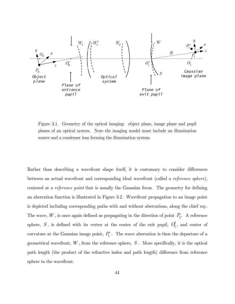
Fig
pla
sou
Rather t
between
centered
an aberra
is depicte
The wav
sphere, S
curvature
geometri
path leng
sphere to
gure 3.1. Ge
nes of an op
urce and a co
than describ
an actual w
at a refere
ation functio
ed including
ve, W , is on
S , is define
e at the Ga
cal wavefron
gth (the pro
o the wavefr
eometry of t
ptical system
ondenser lens
bing a wav
wavefront an
nce point th
on is illustra
g correspond
nce again de
ed with its
aussian imag
nt, W , from
oduct of th
ront.
the optical i
m. Note the
s forming th
vefront shap
nd correspo
hat is usuall
ated in Figu
ding paths w
fined as pro
vertex at
ge point, 1P*
m the refere
e refractive
44
imaging: ob
e imaging m
e illuminatio
pe itself, it
onding ideal
ly the Gaus
ure 3.2. Wa
with and wi
opagating in
the center
* . The wav
ence sphere,
index and
bject plane,
model must i
on system.
is custom
wavefront
ssian focus.
avefront pro
ithout aberr
n the directio
of the exit
ve aberration
S . More
path length
image plane
include an il
ary to cons
(called a re
The geome
opagation to
rations, alon
on of point
t pupil, 1O¢
n is then th
specifically,
h) difference
e and pupil
llumination
sider differe
eference sph
etry for def
o an image p
ng the chief
1.P A refer
, and cente
he departure
it is the op
e from refer
ences
here),
fining
point
f ray.
rence
er of
e of a
ptical
rence
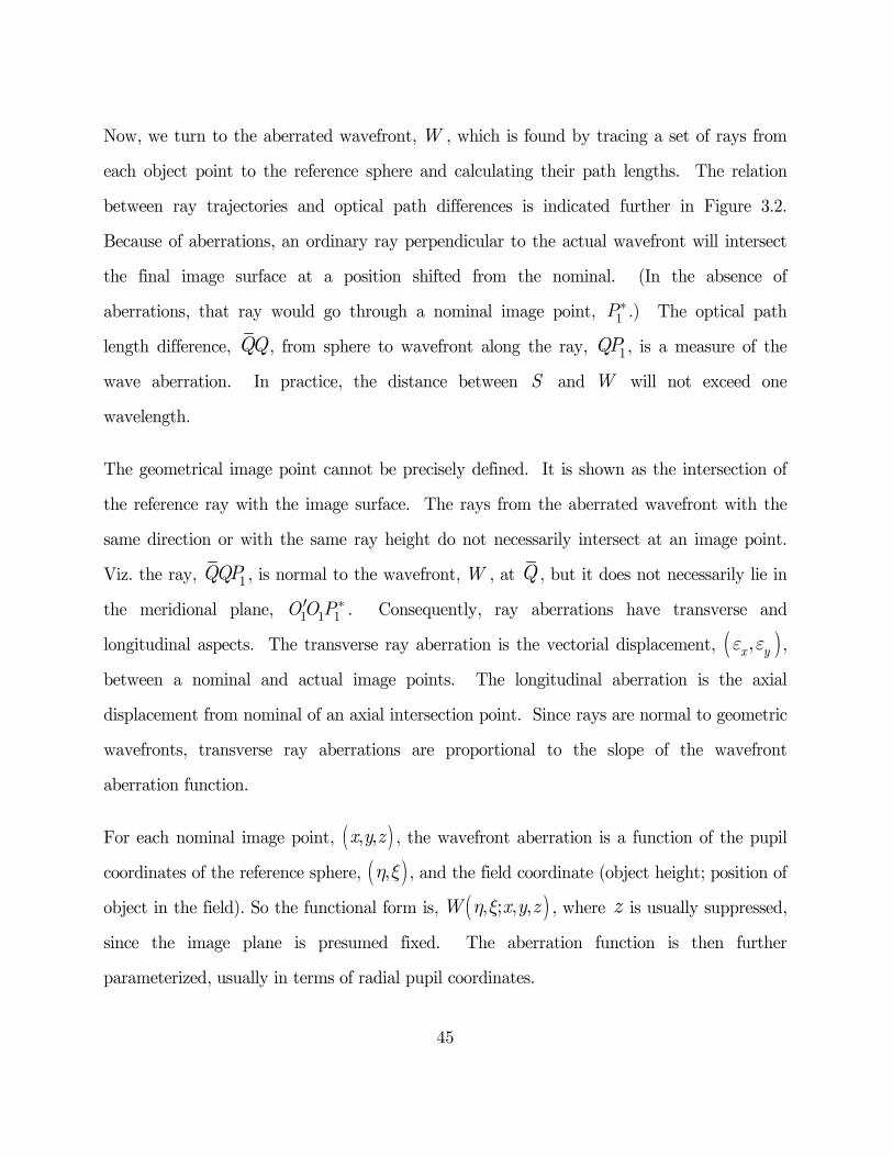
45
Now, we turn to the aberrated wavefront, W , which is found by tracing a set of rays from
each object point to the reference sphere and calculating their path lengths. The relation
between ray trajectories and optical path differences is indicated further in Figure 3.2.
Because of aberrations, an ordinary ray perpendicular to the actual wavefront will intersect
the final image surface at a position shifted from the nominal. (In the absence of
aberrations, that ray would go through a nominal image point, 1P* .) The optical path
length difference, QQ , from sphere to wavefront along the ray, 1QP , is a measure of the
wave aberration. In practice, the distance between S and W will not exceed one
wavelength.
The geometrical image point cannot be precisely defined. It is shown as the intersection of
the reference ray with the image surface. The rays from the aberrated wavefront with the
same direction or with the same ray height do not necessarily intersect at an image point.
Viz. the ray, 1QQP , is normal to the wavefront, W , at Q , but it does not necessarily lie in
the meridional plane, 1 1 1OO P*¢ . Consequently, ray aberrations have transverse and
longitudinal aspects. The transverse ray aberration is the vectorial displacement, ( ),x ye e ,
between a nominal and actual image points. The longitudinal aberration is the axial
displacement from nominal of an axial intersection point. Since rays are normal to geometric
wavefronts, transverse ray aberrations are proportional to the slope of the wavefront
aberration function.
For each nominal image point, ( ), ,x y z , the wavefront aberration is a function of the pupil
coordinates of the reference sphere, ( ),h x , and the field coordinate (object height; position of
object in the field). So the functional form is, ( ), ; , ,W x y zh x , where z is usually suppressed,
since the image plane is presumed fixed. The aberration function is then further
parameterized, usually in terms of radial pupil coordinates.
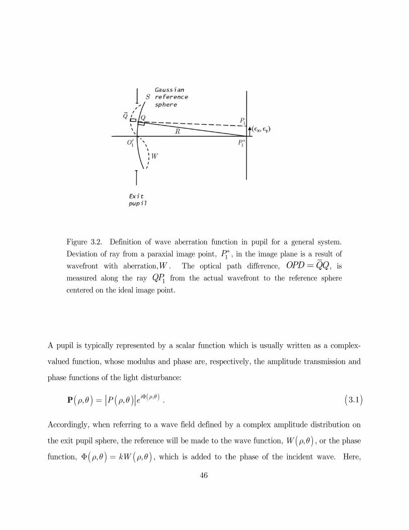
Fig
Dev
wav
mea
cen
A pupil
valued fu
phase fun
Accordin
the exit p
function,
(P
gure 3.2. D
viation of ra
vefront with
asured along
ntered on the
is typically
unction, who
nctions of th
ngly, when r
pupil sphere
( ),r qF =
), Pr q =
Definition of
ay from a pa
h aberration
g the ray Qe ideal image
represented
ose modulus
he light dist
referring to
e, the referen
( ),kW r q=
( ) ( ,, ie rr q F
wave aberr
araxial imag
n,W . Th
1QP from t
e point.
d by a scala
s and phase
urbance:
a wave field
nce will be m
, which is
), .q
46
ation functi
ge point, 1P*
e optical p
the actual w
ar function w
e are, respec
d defined by
made to the
added to th
ion in pupil * , in the ima
path differen
wavefront to
which is usu
ctively, the a
y a complex
e wave funct
he phase of
for a gener
age plane is
nce, OPDo the refere
ually writte
amplitude t
x amplitude
tion, ( ,W r
f the inciden
ral system.
a result of
QQ= , is
ence sphere
en as a com
transmission
e distributio
)q , or the p
nt wave. H
plex-
n and
on on
phase
Here,
( )3.1
47
( )2k p lº , is the angular wavenumber of the wave, or the number of radians of phase per
unit length of the spatial variation in the amplitude. The pupil coordinates will be
normalized to the maximum extent of the aperture, (NA).
3.2 Zernike description of wavefront aberrations
The wave aberration function can be expressed as an expansion into a suitable set of basis
functions, which are functions of the pupil coordinates. A standard way of describing a wave
aberration is to use a Zernike polynomial expansion basis. For a circular pupil, any
continuous wavefront shape, ( ),W r q , may be represented asymptotically by the Zernike
polynomial series expansion:
where i is a polynomial-ordering index, ( ),iZ r q is the ith Zernike circle polynomial
function (e.g., corresponding to the assignment in Table 3.1), and ia its coefficient. Here, r
and q are the radial and angular coordinates in the exit pupil.
In this scheme, one takes the sequence of polynomials { } { }( )21 , 2 cos , 2 sin , 2 1 ,r q r q r -
as a basis for a vector space. The Zernike polynomial coefficients are collected to form a
coefficient vector, a. For the sequence above, the coefficient vector is
{ } { }( )1 2 3 4, , , ,a a a a . One can recreate a wavefront shape by knowing the coefficient
vector and the basis states. Or, one can construct a term corresponding to a specific
polynomial by isolating its coefficient as { } { }( )40 , 0, 0, ,a .
The circle polynomials, as they are called, are universally used for analyzing the aberrations
in lithographic systems. Zernikes are primarily useful for representing wavefront aberrations
( )3.2( ) ( ), , ,i ii
W Zr q a r q¥
= å

48
of systems with conventional circular pupils. For other pupil shapes (annular pupils,
obscured pupils, etc.), other expansions of aberration functions should be used that form
orthogonal sets over the pupil region.
3.2.1 Zernike polynomials
The Zernike polynomials have been described and studied by numerous authors (Zernike,
1934; Kim & Shannon, 1987; Mahajan, 1991; Malacara, 1992; Wyant & Creath, 1992; Born
& Wolf, 1997).
Zernike defined his polynomials as a product of radial and trigonometric functions:
where 0l < and 0n are integers, n l- is even, and
n l . Consequently, only
polynomials with certain ,n l combinations exist. As will be shown, the index n is the
degree of the radial polynomial, and index l is the angular dependence index.
The polynomials ( ),lnV r q are prescribed in complex space. However, the Zernike
polynomials that will be used are the real functions, ( ),mnU r q (Born & Wolf, 1997). The
real polynomials are given by the formulae (m l= ):
so that
( )3.3( ) ( ), , 0 1, 0 2 ,l l iln nV R e qr q r r q p= £ £ £ <
( )3.4( )
( )
1cos
2 ,1
sin2
m m m mn n n n
m m m mn n n n
U V V R m
U V V R mi
r q
r q
-
- -
ìï é ùï = + =ï ê úë ûïíï é ùï = - =ï ê úë ûïî
49
where, again, n ³ m; m takes only values with the same parity as n; and mnR is the radial
polynomial of degree n in terms of the normalized radial coordinates in the pupil plane, r
and q.
The radial functions, ( )mnR r , are polynomials in r and are closely related to Jacobi
polynomials (Zernike, 1934). They are given by
The degree of the radial polynomial ( )mnR r is n and 0 m n£ £ , so it contains the terms
nr , 2nr - , ..., and mr . ( )mnR r is an even or odd polynomial in r, depending on whether
n is even or odd. The normalization is chosen such that ( )1 1mnR = for all values of n
and m , and ( )n nnR r r= .
All Zernike polynomials, ( ),iZ r q , may be ordered with a single index. Instead of
coefficients n and m , a single index, i , is employed. E.g., the order of appearance in the
Table 3.1 follows a singular indexing scheme called “Fringe” ordering (Loomis, 1978; Wyant
& Creath, 1992). Fringe ordering makes use of 2
n m+, which is a single positive value
defined for convenience, and the order of appearance is commensurate to the powers of n .
The polynomials are ordered in ascending values of 2
n m+, and for a given
2
n m+
combination, in descending values of m . For a given ,n m pair, the order of polynomials
with an l value is again descending (e.g., term whose 2m l= = + appears before the
term with 2m l= = - ). These indices and the explicit forms of the aberration
( )3.5( ) ( ) ( ), , ,m m m imn n nU iU R e qr q r q r- =
( )3.6( ) ( ) ( )22
0
!1 .
! ! !2 2
n m
sm n sn
s
n sR
n m n ms s s
r r
-
-
=
-= -
æ ö æ ö+ -÷ ÷ç ç- -÷ ÷ç ç÷ ÷÷ ÷ç çè ø è ø
å

50
polynomials in polar coordinates are listed in Table 3.1. There are other single index
orderings, notably Noll’s (1976) ordering scheme.
The Zernike expansion is often truncated at 36 or 37 terms when describing a wavefront in
lithography, although some applications may require additional terms.
Table 3.1: The first thirty-six Zernike circle polynomials: ( ),iZ r q , i=1...36.
0 0 1 1 Piston
1 1 2 2r cos q Tilt x (about y-axis)
3 2r sin q Tilt y (about x-axis)
0 4 2r2-1 Power
2 2 5 r2 cos 2q Astigmatism x (axis at 0°)
6 r2sin 2q Astigmatism y (axis at 45°)
1 7 (3r3-2r) cos q Coma x
8 (3r3-2r) sin q Coma y
0 9 6r4-6r2+1 Primary Spherical
3 3 10 r3 cos 3q Trefoil x
11 r3 sin 3q Trefoil y
2 12 (4r4-3r2) cos 2q Secondary Astigmatism x
13 (4r4-3r2) sin 2q Secondary Astigmatism y
1 14 (10r5-12r3+3r) cos q Secondary Coma x
15 (10r5-12r3+3r) sin q Secondary Coma y
0 16 20r6-30r4+12r2-1 Secondary Spherical
4 4 17 r4cos 4q Tetrafoil x
( )Polynomial cos
sinmnR mr q
ì üï ïï ïí ýï ïï ïî þi
m
2
n m+Aberration name
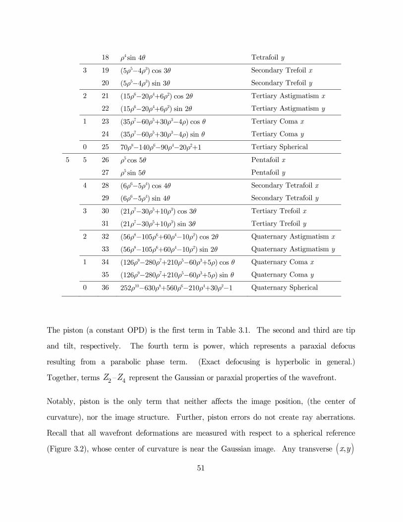
51
18 r4 sin 4q Tetrafoil y
3 19 (5r5-4r3) cos 3q Secondary Trefoil x
20 (5r5-4r3) sin 3q Secondary Trefoil y
2 21 (15r6-20r4+6r2) cos 2q Tertiary Astigmatism x
22 (15r6-20r4+6r2) sin 2q Tertiary Astigmatism y
1 23 (35r7-60r5+30r3-4r) cos q Tertiary Coma x
24 (35r7-60r5+30r3-4r) sin q Tertiary Coma y
0 25 70r8-140r6-90r4-20r2+1 Tertiary Spherical
5 5 26 r5cos 5q Pentafoil x
27 r5sin 5q Pentafoil y
4 28 (6r6-5r4) cos 4q Secondary Tetrafoil x
29 (6r6-5r4) sin 4q Secondary Tetrafoil y
3 30 (21r7-30r5+10r3) cos 3q Tertiary Trefoil x
31 (21r7-30r5+10r3) sin 3q Tertiary Trefoil y
2 32 (56r8-105r6+60r4-10r2) cos 2q Quaternary Astigmatism x
33 (56r8-105r6+60r4-10r2) sin 2q Quaternary Astigmatism y
1 34 (126r9-280r7+210r5-60r3+5r) cos q Quaternary Coma x
35 (126r9-280r7+210r5-60r3+5r) sin q Quaternary Coma y
0 36 252r10-630r8+560r6-210r4+30r2-1 Quaternary Spherical
The piston (a constant OPD) is the first term in Table 3.1. The second and third are tip
and tilt, respectively. The fourth term is power, which represents a paraxial defocus
resulting from a parabolic phase term. (Exact defocusing is hyperbolic in general.)
Together, terms 2Z – 4Z represent the Gaussian or paraxial properties of the wavefront.
Notably, piston is the only term that neither affects the image position, (the center of
curvature), nor the image structure. Further, piston errors do not create ray aberrations.
Recall that all wavefront deformations are measured with respect to a spherical reference
(Figure 3.2), whose center of curvature is near the Gaussian image. Any transverse ( ),x y

52
displacement with respect to the Gaussian image appears as a wavefront tilt and any
longitudinal ( )z displacement appears as a defocusing term. To completely define a
spherical reference, the position of center of curvature and the radius of curvature are also
needed. Any change in this radius of curvature introduces a modification in the piston term,
a constant. The tilt terms represent a shift of focus but do not imply departure from
sphericity. They can be eliminated by appropriate choice of focus, which corresponds to a
shift at the center of the reference sphere.
The next five terms of the series are the so-called third-order aberrations, because of their
relation to Seidel (classical) and 3rd order transverse aberrations. They are Zernike terms:
5Z and 6Z (classical astigmatism plus defocus made up of one or more classical
aberrations); 7Z and 8Z (classical primary coma plus tilt); and 9Z (third-order classical
primary spherical term 4r combined with defocus term 2r ).
In all cases, with the exception of the piston term, image quality will be degraded compared
to that of an equivalent unaberrated system. The piston term is simply a constant phase
shift across the pupil, and the PSF is the same as that of an unaberrated system. It does
not affect the shape of the wavefront and, consequently, has no effect on image. The tilt
modes are linear phase gradients across the pupil and result in an x or y shift in the PSF,
but do not affect its size or shape.
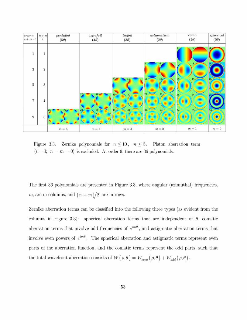
Figure
( 1i =
The first
m, are in
Zernike a
columns
aberratio
involve e
parts of
the total
3.3. Zern
; n m= =
t 36 polynom
n columns, a
aberration t
in Figure
on terms tha
even powers
the aberrat
wavefront a
nike polynom
0) is exclud
mials are pr
and (n m+
erms can be
3.3): sphe
at involve o
s of ime q . T
tion function
aberration c
mials for n
ded. At orde
resented in F
) 2 are in r
e classified i
erical aberra
odd frequenc
The spherica
n, and the c
consists of W
53
10n £ , m £
er 9, there ar
Figure 3.3, w
rows.
into the foll
ation terms
cies of ime q
al aberratio
comatic ter
( ),W Wr q =
5£ . Pisto
re 36 polyno
where angu
lowing three
s that are i
, and astigm
on and astig
rms represen
( ),evenW r q
on aberratio
omials.
ular (azimut
e types (as e
independent
matic aberra
gmatic term
nt the odd
( ,oddW r q+
on term
hal) frequen
evident from
t of q, com
ation terms
s represent
parts, such
)q .
ncies,
m the
matic
that
even
that

54
Characterizing aberrations in groups, up to and including a certain order (e.g., with primary
aberrations, which are the terms up to the third order) is convenient. Succeeding groups of
higher order terms are, again, fifth, seventh and ninth order aberrations, corresponding to
rows in the structure of Figure 3.3. The order of a certain term is given by the value
1n m+ - . It can be shown that the order is always odd. There are five aberration terms
of third order, which are 5Z through 9Z . There are seven aberration terms of fifth order
( 10Z — 16Z ). Likewise, terms 17Z through 25Z represent seventh-order aberrations; terms
26Z through 36Z represent ninth order aberrations, and so on.
Figure 3.4 offers another useful view of the Zernike polynomial functions ( ),iZ r q recast
such that the radial degree, n , changes vertically, and angular frequency, m, changes
horizontally. This form offers the same geometry as found in the definition in Equation
(3.4).
It will be shown next that it is also possible to classify Zernike polynomials according to
parity.
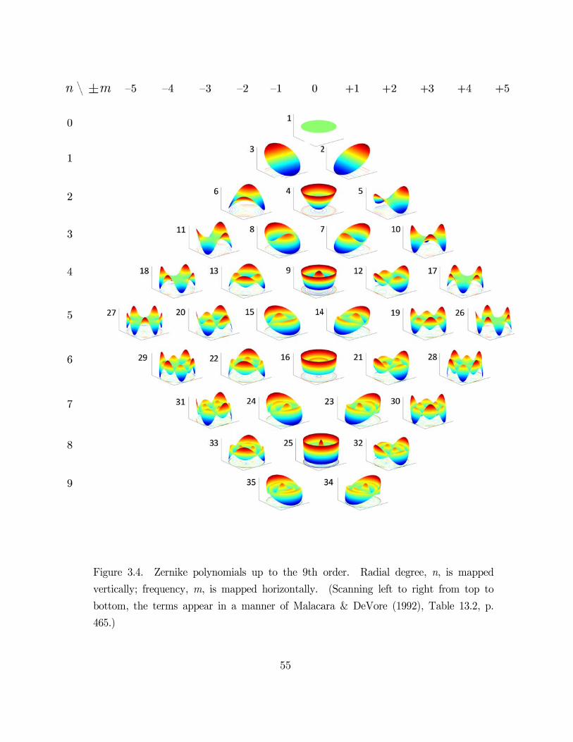
Fig
ver
bot
465
gure 3.4. Z
tically; frequ
ttom, the te
5.)
ernike polyn
uency, m, is
erms appear
nomials up
s mapped h
in a manne
55
to the 9th
orizontally.
er of Malaca
order. Rad
(Scanning
ara & DeVo
dial degree,
left to righ
ore (1992),
n, is mapp
ht from top
Table 13.2,
ped
to
p.
56
3.2.2 Rotation through parity states
Symmetrical versus antisymmetrical aberrations grouping is brought about by the parity
property of the Zernike polynomials.
Let { }P ⋅ be a parity operator which acts upon a function, f . If the function, f , has a
definite state of parity then it can be represented as ( ) ( ){ }f x P f x = ; { }P ⋅ has a
multiplicative action of either 1 or –1. If ( ) ( )f x f x- = , the function is even; and if
( ) ( )f x f x- = - , the function is odd.
Any function, ( )g x , can be resolved into two parity components, where ( )g x+ is even and
( )g x- is odd, according to:
The sum of the even and odd components restores the original component.
Recall that the Euler identity cos sinixe x i x= + resolves the complex exponential into
functions of cosine (even) and sine (odd) parity. Similarly, a complex exponential equation,
( ),lnV r q , is resolved into two distinct parity states:
where m l= . Consequently, Zernike polynomials are paired functions of opposite parity
(see Table 3.2 below), except for rotationally invariant polynomials, ( )0 ,nU r q , that do not
have parity partners. An example of parity states is given in Figure 3.5.
( )3.7( ) ( ) ( ) ( ) ( ) ( )1 1and .
2 2g x g x g x g x g x g x+ -é ù é ù= + - = - -ë û ë û
( )3.8( ) ( ) ( ) ( ), cos and , sin ,m m m mn n n nU R m U R mr q r q r q r q-= =
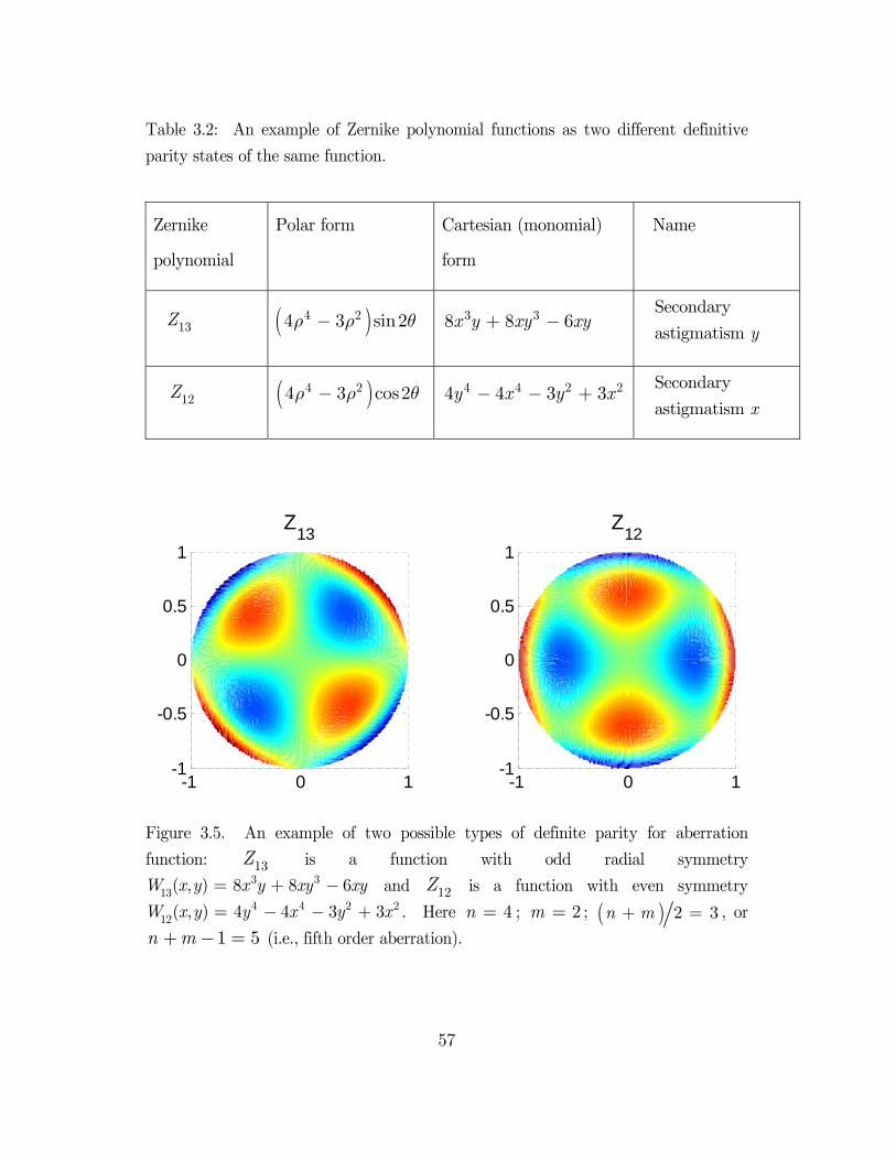
57
Table 3.2: An example of Zernike polynomial functions as two different definitive
parity states of the same function.
Zernike
polynomial
Polar form Cartesian (monomial)
form
Name
Secondary
astigmatism y
Secondary
astigmatism x
Figure 3.5. An example of two possible types of definite parity for aberration
function: 13Z is a function with odd radial symmetry 3 3
13( , ) 8 8 6W x y x y xy xy= + - and 12Z is a function with even symmetry 4 4 2 2
12( , ) 4 4 3 3W x y y x y x= - - + . Here 4n = ; 2m = ; ( ) 2 3n m+ = , or
1 5n m+ - = (i.e., fifth order aberration).
-1 0 1-1
-0.5
0
0.5
1
Z12
-1 0 1-1
-0.5
0
0.5
1
Z13
( )4 24 3 sin2r r q-
( )4 24 3 cos2r r q-
13Z
12Z
3 38 8 6x y xy xy+ -
4 4 2 24 4 3 3y x y x- - +
58
Compared to 12Z , there is no simple symmetry in the 13Z surface about the x and y axes:
However, there is a more subtle symmetry with
which follows from the aberration function separability in polar coordinates ( ),r q .
This odd/even parity describes rotational symmetry of aberration function due to its
frequency, m , being odd/even. As we consider the structure of an image within an
aberrated system, both even and odd aberrations in terms of frequency, m , are classified as
such, due to the z or ( ),x y effect on image symmetry. When 0m = , there is rotational
symmetry in xy , but the diffraction image is not symmetrical with respect to the plane
0z = . When m is odd, the intensity distribution is symmetrical with respect to the plane
0z = , and the z -axis is the m -fold axis of symmetry with respect to the pattern in plane
0z = . When m is even, the z -axis is a 2m -fold axis of symmetry with respect to a
pattern in the plane 0z = , and the intensity is a result of reflection in plane 0z = and
additional rotation at an angle p/m about the z -axis (Born & Wolf, 1999).
If we consider the amplitude and intensity scans of the 3D PSF, we will see that symmetrical
aberrations like spherical impede the longitudinal ( )z symmetry of the 3D PSF, while
asymmetrical aberrations like coma impede the transverse ( ),x y symmetry. For example,
intensity (amplitude distribution) through focus is bent to the shape of a banana for 7Z
(Flagello et al., 1997).
( )3.9( ) ( ), ( , ), , ( , ).W x y W x y W x y W x y¹ - ¹ -
( )3.10( ) ( ), ( , ), , ( , ),W x y W x y W x y W x y= - - - = -
59
3.2.3 Orthogonality property
The Zernike polynomials are often used because of their unique and desirable properties
derived from their orthogonality.
These polynomials form complete orthonormal sets over the unit circle (exit pupil with
radius one) (Born & Wolf, 1999). The Zernike polynomials are complete in the sense that
any wavefront function ( ),W r q of degree n can be expressed as a linear combination of
Zernike circular polynomials. Polynomials ( ),mnU r q are orthogonal functions over the unit
circle in a continuous fashion that satisfy
with r being the normalized radial coordinate. The Kronecker delta, nnd ¢ , is zero if n is
different from n ¢ . Because the angular functions, ime q , are already orthogonal, it follows
that radial functions must satisfy the following orthogonality (and normalization) condition:
The average value of each term over the unit circle is zero. It should be pointed out that
these polynomials are orthogonal only if the pupil is circular and without obscuration. Since
the Zernike polynomials are orthogonal, their partial derivatives in x and y are orthogonal.
Their Fourier transforms are also orthogonal (Dai, 2006).
In addition to orthogonality and the above mentioned simple rotational symmetry properties
of Zernike polynomials, another useful property is that the mathematical form of the
polynomial is preserved when a rotation with a pivot at the center of the unit circle is
( )3.11( ) ( ) ( )1 2
0 0, , ,
2 1m mn n nn mmU U d d
n
p pr q r q r r q d d¢
¢ ¢ ¢=+ò ò
( )3.12( ) ( ) ( )1
0
1.
2 1m mn n nnR R d
nr r r r d¢
¢ ¢=+ò

60
applied to the wavefront function. Specifically, the polynomial is invariant in form with
respect to rotation of the axes about the origin, i.e. about the optical axis.
3.2.4 Image quality criteria with aberrations
Where, again, W is the wave aberration function, and F the phase function:
The amount of aberration that can be tolerated in a certain optical system depends on the
criteria used for image quality. A simple criterion is the Strehl ratio, which represents the
effect of aberration on central irradiance. It is defined as the ratio of irradiance at the center
of a reference sphere (with respect to which the aberration is defined) with and without
aberration:
where IF is the value at zero of a diffraction pattern formed by an aberrated system and
0IF= is that of an image in an aberration-free system. Strehl intensity is the on-axis
intensity in an optical system with aberration. The point of maximum intensity (peak
intensity) in a given aberrated system is not necessarily the Strehl intensity; diffraction focus
does not necessarily occur on axis.
The Strehl normalized intensity, S , in the image region, may be written as
( )3.13( ) ( )2, , .W
pr q r q
lF =
( )3.14( )
( )0
0,
0
IS
IF
F=
=
61
which is an approximate form for the Strehl ratio as given by Nijboer (1943).
The average value of the nth power of W is
Because the wavefront aberration is nominal, the third and higher powers of kW can be
neglected, and we can write
where l is the wavelength, W is mean wavefront OPD relative to spherical wave,
2W is the expected value of 2W , and 2
W is the square of the expected value of the
aberration function W . The quantity in the square brackets is the mean-square deformation
of the wavefront or the variance of the aberration function:
Equation (3.17) can be rewritten as
( )3.15( )
( ) ( )
21 2
20 0
2
20
22
2
1
1 1
!
1 1 11 ,
2 !
ikW
n
n
n
S e d d
ikW d dn
ikW ikW ikW d dn
p
r r qp
r r qp
r r qp
¥
=
=
é ùê ú= ê úê úë û
é ùê ú= + + + + +ê úë û
ò ò
åòò
òò
( )3.16( )
1 2
1 20 0
1 2 0 0
0 0
, 1, 1,2.
n
n nW d d
W W d d nd d
pp
p
r q r r qr r q
pr r q= = =
ò òò ò
ò ò
( )3.172 2
22 2 21 21 1 ,
2S ik W k W W W
pl
æ ö é ù÷ç» + - » - -÷ç ê ú÷÷ç ë ûè ø
( )3.182 2 22 2 22 .W W W W W W W W Ws é ù= - = + - = -ë û
62
Given that 1) the deviation from the unit Strehl ratio for small aberrations is the variance
2sF of the phase departure, F , of the focusing wave over the exit pupil of the optical system;
2) the orthogonality of the individual aberrations simplifies the calculations that involve
integration over pupil area; and 3) 2Ws is a simple weighted sum of squares of the Zernike
expansion coefficients, the Equation (3.19) can be rewritten as
Because the wavefront variance is equal to the sum of the Zernike coefficients squared,
Equation (3.20) shows that the Strehl ratio is expressed in terms of the expansion coefficients
in Equation (3.2) and that each individual aberration reduces the Strehl ratio independently.
The amounts of different aberrations corresponding to a Strehl level will vary, but an
approximation is sufficient where any combination of aberrations must correspond to a
mean-square wavefront aberration of ( )250l or less for the state-of-the art high-resolution
lithographic objective.
In lithography, the system aberration tolerance is mainly set with following three metrics of
system performance: Strehl criterion, the peak-to-valley (PV), and root-mean-square
wavefront error (RMS OPD). PV quantity is simply the difference between the maximum
and the minimum values of the phase (or a total range), and RMS OPD is the average phase
difference over the aperture area (departure of wavefront from a reference sphere). The
RMS wavefront error is determined by 2W and is equal to the standard deviation Ws
only when 0W = . The RMS OPD wavefront error is measured in wavelengths. The
total RMS wavefront error value is directly related to the Zernike coefficients, ia , which are
( )3.192
2 221 1 .WS
ps s
l F
æ ö÷ç- = -÷ç ÷÷çè ø
( )3.202
2
2
21 .i
i
Sp
al
¥
=
æ ö÷ç= - ÷ç ÷÷çè ø å

63
related to image quality via the Strehl ratio, S . For a given value of Strehl ratio, the
tolerance for an aberration increases as its standard deviation decreases. Note also for a
given RMS wavefront error level, the PSF usually worsens as the term order increases.

64
4. Phase wheel aberration monitor
4.1 Overview
Having discussed geometric aberration theory in Chapter 3, in the present chapter we
consider the diffraction theory of aberrations, a necessary part of system evaluation.
Analysis in §3.1 introduced the basic concept of the wavefront in the pupil, which now needs
to be extended to image evaluation to allow us to quantify the contribution of a particular
aberration to the image.
Section 4.1, starts with some considerations concerning the general problem of image
evaluation in the lithographic image. Section 4.1.1 looks at how imaging characteristics can
be evaluated on the basis of wavefront aberrations in lens pupil, in order to obtain a
qualitative measure for the discrepancy between the actual image and the unaberrated
image. Some frequently used image quality criteria are properties of the complex pupil
function; others are obtained from the optical transfer function (OTF) or the point spread
function (PSF). This discussion will be the subject of Sections 4.1.2, 4.1.3, and 4.1.4. In
§4.1.2, linear systems analysis is outlined, and in §4.1.3, consideration of partial coherence is
given. In §4.1.4, the special case of image of a strong phase edge for system identification is
treated.
65
Although the Zernike aberrations give an idea of the overall capability of the system, the
individual aberrations are nontrivial to identify from the final image. By examining the
effect that an optical system has on select objects, such as point objects, periodic objects
(line gratings), radial gratings (Siemens star), line objects, or edge objects, etc. an evaluation
of the system performance can be made. These concepts will be applied to the design of
phase wheel test targets and their properties and relevance to system evaluation discussed in
§§4.1.5 – 4.1.6.
In Section 4.2, the starting point of the phase wheel monitor concept is set forth. Section
4.2.1 gives image formation steps and Section 4.2.2 gives details on the parameterized
description of phase wheel images. Section 4.3 contains the application details of phase
wheel monitor concept; special emphasis is given to the image processing of phase wheel
images. The final section, §4.4, gives a summary of this image based concept.
4.1.1 Image evaluation
This imaging problem deals with images that have been degraded by the presence of
aberrations as well as by the limited resolution of the system due to diffraction.
This can be illustrated in terms of an image produced by the system of a grating object with
sinusoidal intensity distribution. Let the intensity transmittance associated with such an
object be
Where x is a coordinate in the object plane and 0x is a spatial frequency. Then the
diffraction image of this sinusoidal object will be of the form
( )4.1( ) { }0 0, 1 cos2 ,I x y I xpx= +
66
where quantity 0I ¢ is the average image irradiance, m is modulation or contrast, 0y is
arbitrary phase constant. The intensity distribution that appears in image is similar to the
object but reduced in contrast according to the factor 1m < , due to a modulation transfer
function (MTF), and its phase is shifted by the amount 0y , due to a phase transfer function
(PTF). The phase shift has the effect of distorting the relative position of image features
such as edges rather than simply blurring them. The image quality can thus be specified by
the factors m and 0y , or more generally, by an optical transfer function ( )H x :
where the modulation transfer function is the modulus of the OTF and the phase transfer
function is its argument, both linked to aberrations associated with the system. The
reduction in contrast and changes in the phase of the sinusoidal spatial frequency
components contribute to the overall image degradation. Thus, the system OTF is a
complete measure of image quality in terms of contrast and resolution in the presence of
aberrations. This is true even if the system is aberration free, in which case the OTF is real
and the PTF is zero. The OTF is a function of the spatial frequency x as well as of the
focal setting (defocusing) and illumination bandwidth.
The condition under which Equation (4.2) represents the image intensity distribution is that
the illumination in the object is perfectly incoherent, in other words when it is a linear
system. The physical models of optical imaging aim, whenever possible, to provide a linear
systems description. We will consider both linear and nonlinear system description aspects
next.
( )4.2( ) ( ){ }0 0 0, 1 cos2 ,I x y I m xpx y¢¢ = + +
( )4.3( ) ( ) ( ) ( ) ( )0 0
0, , ,im H H H e xx x x x
x y x x x Y= =
= = Y =
67
4.1.2 Linear system description – the incoherent and coherent limits
Imaging systems where diffraction effects are important are called diffraction-limited.
Diffraction-limited imaging systems are typically treated by Fourier optics, where an optical
system is viewed as a linear system or a black box fully characterized by its impulse response
(or point spread function).
The one-dimensional linear transformation describing the transition from object to image has
the form
where f is the input signal which represents an object distribution, g is the output signal
which represents an image distribution and ( )1h x is the impulse response of the optical
system, i.e. the output at x due to an impulse at 1x . This description is correct in the case
of completely coherent or completely incoherent illumination (Saleh, 1979). In an optical
system that uses incoherent illumination, f and g denote light intensities. If spatially
coherent illumination is used, f and g denote optical fields.
With coherent optical imaging, field distribution in the image plane is the object field
convolved with the ( )h x function:
where the symbol Ä denotes a convolution operation. The ( )g x is complex disturbance;
however, the detection process can only measure the image intensity given by the square
modulus of the complex amplitude:
( )4.4( ) ( ) ( )1 1 1 ,g x f x x h x dx+¥
-¥
= -ò
( )4.5( ) ( ) ( ),g x f x h x= Ä

68
For coherent imaging there is no linear relation between image intensity ( )I x and the
object intensity ( ) 2f x .
In the case of incoherent illumination, the image formation can be described as
which is equivalent to a linear system whose PSF is ( ) 2h x and input is ( ) 2
f x . That is,
for an incoherent image, intensity in the image plane results from a convolution of intensity
in the object plane with the PSF of the optical system:
Hence, this system is linear with respect to the light intensity.
If by ( )h x we denote the coherent PSF of the system, we have the incoherent PSF of the
same system as ( ) ( ) ( )2h x h x h x*= . Mathematically it is the complex square of the
amplitude distribution in the image. The point spread function describes the optical system
response to an impulse, the actual image produced for a point object, and fully accounts for
the effects of both diffraction and aberrations. It will be shown next that PSF is a function
of the wavefront aberration and can be obtained by taking inverse Fourier transform of the
complex pupil function ( ),x hP on the exit pupil:
where the integration is made over the exit pupil area S , and ( ),x y are coordinates in the
focal plane. It effectively describes the magnitude and phase of the light at the focal plane.
( )4.6( ) ( ) ( ) ( )2 2.I x g x f x h x= = Ä
( )4.7( ) ( ) ( )2 21 1 1 ,g x f x x h x dx
¥
-¥
= -ò
( )4.8( ) ( ) ( ) ( )2 2.I x g x f x h x= = Ä
( )4.9( ) ( ) ( )2, , ,i x yh x y e d dp x hx h x h+ +
S
= òò P
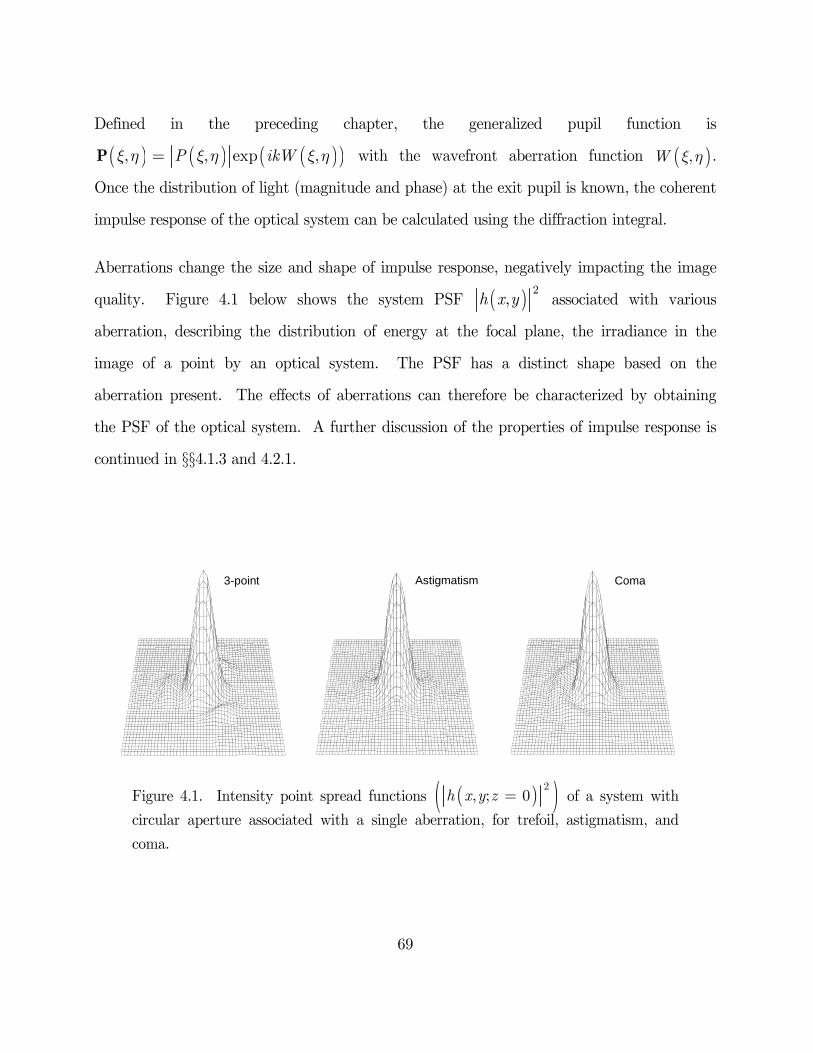
69
Defined in the preceding chapter, the generalized pupil function is
( ) ( ) ( )( ), , exp ,P ikWx h x h x h=P with the wavefront aberration function ( ),W x h .
Once the distribution of light (magnitude and phase) at the exit pupil is known, the coherent
impulse response of the optical system can be calculated using the diffraction integral.
Aberrations change the size and shape of impulse response, negatively impacting the image
quality. Figure 4.1 below shows the system PSF ( ) 2,h x y associated with various
aberration, describing the distribution of energy at the focal plane, the irradiance in the
image of a point by an optical system. The PSF has a distinct shape based on the
aberration present. The effects of aberrations can therefore be characterized by obtaining
the PSF of the optical system. A further discussion of the properties of impulse response is
continued in §§4.1.3 and 4.2.1.
Figure 4.1. Intensity point spread functions ( )( )2, ; 0h x y z = of a system with
circular aperture associated with a single aberration, for trefoil, astigmatism, and
coma.
3-point Coma Astigmatism
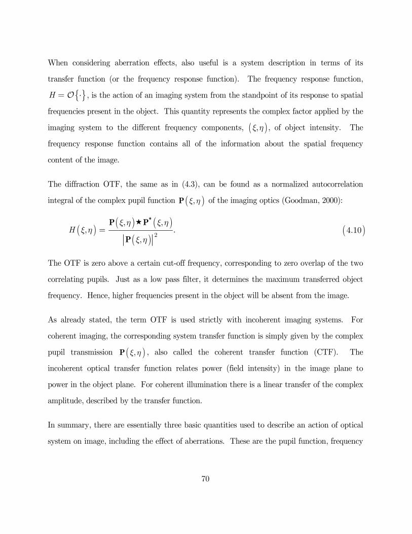
70
When considering aberration effects, also useful is a system description in terms of its
transfer function (or the frequency response function). The frequency response function,
{ }H = ⋅ , is the action of an imaging system from the standpoint of its response to spatial
frequencies present in the object. This quantity represents the complex factor applied by the
imaging system to the different frequency components, ( ),x h , of object intensity. The
frequency response function contains all of the information about the spatial frequency
content of the image.
The diffraction OTF, the same as in (4.3), can be found as a normalized autocorrelation
integral of the complex pupil function ( ),x hP of the imaging optics (Goodman, 2000):
The OTF is zero above a certain cut-off frequency, corresponding to zero overlap of the two
correlating pupils. Just as a low pass filter, it determines the maximum transferred object
frequency. Hence, higher frequencies present in the object will be absent from the image.
As already stated, the term OTF is used strictly with incoherent imaging systems. For
coherent imaging, the corresponding system transfer function is simply given by the complex
pupil transmission ( ),x hP , also called the coherent transfer function (CTF). The
incoherent optical transfer function relates power (field intensity) in the image plane to
power in the object plane. For coherent illumination there is a linear transfer of the complex
amplitude, described by the transfer function.
In summary, there are essentially three basic quantities used to describe an action of optical
system on image, including the effect of aberrations. These are the pupil function, frequency
( )4.10( )( ) ( )
( ) 2
, ,, .
,H
x h x hx h
x h=
*P P
P
71
response function, and impulse response function. The relationships among these different
functions and computational domains are illustrated in Figure 4.2 below.
Figure 4.2. Relations that hold between the various 1st order optical functions used
for describing the linear optical systems. If partial coherence of illumination must be
taken into account, nonlinear system representations must be considered (§4.1.3).
The pupil function ( ),x hP describes the magnitude and phase of the light in the pupil
plane. The modulus squared of ( ),x hP gives the radiance distribution of light over the
pupil. The phase of the pupil function is proportional to the wavefront OPD. It is the
frequency response for coherent illumination. The optical transfer function ( ),H x h is the
normalized autocorrelation of the complex pupil function; it is also the Fourier transform of
the incoherent system PSF. Whereas the CTF is the Fourier transform of the coherent PSF,
the OTF is the Fourier transform of the squared amplitude of the PSF of the system. For
these operations the linearity condition is fulfilled and a Fourier transform is a mutual
relation between the main functions.
( )( ) ( ) ( )
( ) ( )2
Autocorrelation,
1
2
,,
,
, ,
ikW HP e
h x y h x y
x h
x hx h
x h
-
=¾¾¾¾¾¾
¾¾¾¾¾¾
P
72
The effect of aberrations on the PSF is to reduce the magnitude of the central peak, with
extra energy being distributed into the diffraction rings, so the contrast of the diffraction
image is further reduced. The effect of aberrations on the OTF is to reduce contrast at
every spatial frequency above the diffraction limit at that frequency. This is because the
OTF describes the amplitude with which each frequency is transferred, and thus, the
contrast of the object details formed by that frequency. The effect of aberrations in the
incoherent case is not simply a phase modulation as in the coherent one,—the aberrations
can also produce variations of the modulus of the OTF.
One approach for describing the system OTF is by taking the image measurements and
studying the contribution of aberration types to the distortions in image. Careful
consideration is needed when selecting the objects for system characterization, because it
impacts how the aberration measurement is done. For example, if an object considered
consisted of all spatial frequencies, then the OTF is the Fourier transform of the image.
Such an object is called a point object and its image is the PSF.
A further complication encountered in testing is that the image is generally not given by a
simple Fourier transformation of the transfer function multiplied by the object spectrum.
Rather, in many cases, and these include examples in lithography, the transfer of
modulations involves a number of nonlinear processes. The coherence properties of the light
source, i.e. the illumination conditions, have to be considered. Illumination has a significant
influence on imaging. Image formation can be treated as linear only when illumination is
fully coherent or incoherent, however, the case of partially coherent illumination is the more
frequent one in lithography, and the effect of coherence must be discussed together with the
effect of aberration (Singer, Totzek, & Gross, 2005).
73
The mathematical conditions for applying the Fourier transform to calculate system transfer
function include linearity assumption, which breaks down when the phase in beam from one
source point depends on another source point (coherence). Partial coherence will tend to
violate the conditions necessary (linearity assumption) for applying the Fourier transform to
calculate the OTF. Nonlinear formalism is needed for model of a system. A class of
nonlinear transformations, called bilinear, must be considered (Saleh, 1979).
The overall object–image relation is highly nonlinear. In addition to the partially coherent
imaging process being nonlinear, the photoresist detection step is also considered nonlinear.
The significance of nonlinear system description is discussed in the following section.
4.1.3 Nonlinear system description – the effect of partial coherence on
imaging
We will now consider a system producing partial coherent images. We assume that the
system is space-invariant; in practice, optical lithography imaging systems are seldom space-
invariant over the full image field (Singer et al., 2005). It is possible to derive a model for
the image formation in cases where there is coherence between the various image
contributions using a nonlinear system description. The mathematical descriptions of a
partially coherent imaging system in the two domains are the following.
The 1D imaging equation is given by a two-dimensional convolution integral
where the 2-nd order kernel ( )1 2,k x x is a higher-order impulse response of the system. The
input ( )f x is generally complex, but output ( )g x is real. It is a model for nonlinear
( )4.11( ) ( ) ( ) ( )1 2 1 2 1 2, ,g x f x x f x x k x x dx dx+¥
*
-¥
= - -ò ò
74
behavior of many optical transformations. It is well generalized for higher dimensions and
can represent a wide range of systems (Saleh, 1979).
In a partially coherent system, the double impulse response depends on the degree of
coherence of the illumination in the object plane ( )xg and the coherent impulse response
( )h x of the system:
Equation (4.12) represents the kernel of a system that describes diffraction of partially
coherent light of degree of coherence ( )xg . If ( )1 2 1x xg - = , i.e. coherence function
degenerates to a constant, we recover Equation (4.6). Incoherent illumination gives a special
case of ( ) ( )1 2 1 2x x x xg d- = - and we recover Equation (4.8).
A complete (meaning for any input) partially coherent system description cannot be given
by a 1D transfer function. That is for a 1D nonlinear system, a 2D transfer function is
needed, which depends on optical system as well as on illumination. This bilinear transfer
function (BTF) is defined as
The depends on the imaging system coherent transfer function ( )xP and the
illumination cross-spectral density ( )xG , which is a Fourier transform of ( )xg . It is a
generalization of the idea of a transfer function in linear system. It is also called the
“transmission cross-coefficient” (TCC) (Hopkins, 1953). Since is a 2D function for a 1D
object, i.e. is a function of 2 frequencies, it is 4D for a 2D object and consequently is more
difficult to treat.
( )4.12( ) ( ) ( ) ( )1 2 1 2 1 2, .k x x h x h x x xg*= -
( )4.13( ) ( ) ( ) ( )1 2 1 2, .dx x x x x x x x+¥
*
-¥
= G - +ò P P
75
The 1D image ( )g x that depends bilinearly on the object transmission spectrum can be
rewritten as
And we have the imaging system that is characterized completely by the bilinear transfer
function ( )1 2,x x , whose 2D Fourier inverse is the double-impulse response function
( )1 2,k x x .
Analysis of TCC in frequency domain proves insightful (Saleh, 1979). For coherent light,
( ) ( ) ( )1 2 1 2,x x x x*= -P P and k factorizes in the form ( ) ( ) ( )1 2 1 2,k x x h x h x*= . For
incoherent light, ( ) ( )1 2 1 2, Hx x x x= + , where ( )H x is a Fourier transform of ( ) 2h x ,
and ( ) ( ) ( ) ( )1 2 1 2 1 2,k x x h x h x x xd*= - (i.e. the double-impulse response is zero unless
the 2 impulses coincide). The ( ), 0x is the so-called linear part of TCC and gives the
OTF (incoherent transfer function). Unlike the OTF, one cannot characterize a bilinear
transfer function by use of pure sinusoidal inputs. In reality this amounts to saying that one
cannot characterize a nonlinear system with a single linear transfer function. Note that
( ) ( ) ( ) 2,x x x x- = G Ä P represents a uniform term that results from a harmonic input.
It is independent of the phase of ( )xP , that is independent of defocusing and aberration in
an optical system. Explicitly recognizing this fact and the nonlinearity in , one needs to
use special targets and setup for the purpose of studying a nonlinear response of the system
with aberration to a given input. Wavefront errors, in general, lead to a complex TCC and
cause additional phase modulations in image intensity (Singer et al., 2005).
Partially coherent imaging system description is typically difficult to treat analytically.
Since ( )I x varies in a fairly complicated way, and the formulae that describe the partial
coherent imaging have a quite complicated nature, the resultant integration cannot, as a
( )4.14( ) ( ) ( ) ( ) ( )1 221 2 1 2 1 2, .ixg x F F e d dp x xx x x x x x
+¥+ -*
-¥
= ò ò
76
rule, be carried out explicitly and use of numerical integration techniques is necessary. But
for a few simple cases we can perform exact calculations (as in §4.1.4).
We can now formulate the wavefront reconstruction problem. Our objective is to study the
problem of nonlinear system identification, i.e. finding a pupil distribution that corresponds
to a given image distribution in the presence of aberrations. The measured values of the
image ( )g x consist of squared-magnitude (intensity), thresholded by the photoresist film
detector. When we include the photoresist in the imaging system and regard the resist
image as the final output image, we encounter another case of nonlinear imaging where
output is nonlinearly related to the detected optical intensity. Thus we have a nonlinear
(partial coherent) system followed by a nonlinear detector. The overall object–image
relation is nonlinear, and needs to be included when modeling the system. To examine the
nonlinearity of the image formation due to the partially coherent optical system and the
effects of phase variations in the pupil, the test objects will be tailored to characterize the
system. Because the second-order system response cannot be analyzed a single-frequency
sinusoidal object, a phase object of constant amplitude and only phase variations is better
suited for system characterization.
4.1.4 Imaging of a phase edge
Certain phase objects can be very sensitive to aberrations, provided the phase difference is
not small and a low coherence illumination is used. Thus, by using strong phase objects as
test patterns, it may be possible to reconstruct the phase error in the pupil. In the
incoherent image, the phase structure cannot be resolved, but when illumination is
increasingly more coherent it is possible to achieve high contrast images of strong phase
objects. Sensitivity of the phase edge is expected to be greater than of any binary edge. The
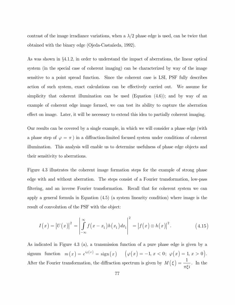
77
contrast of the image irradiance variations, when a l/2 phase edge is used, can be twice that
obtained with the binary edge (Ojeda-Castañeda, 1992).
As was shown in §4.1.2, in order to understand the impact of aberrations, the linear optical
system (in the special case of coherent imaging) can be characterized by way of the image
sensitive to a point spread function. Since the coherent case is LSI, PSF fully describes
action of such system, exact calculations can be effectively carried out. We assume for
simplicity that coherent illumination can be used (Equation (4.6)); and by way of an
example of coherent edge image formed, we can test its ability to capture the aberration
effect on image. Later, it will be necessary to extend this idea to partially coherent imaging.
Our results can be covered by a single example, in which we will consider a phase edge (with
a phase step of j p= ) in a diffraction-limited focused system under conditions of coherent
illumination. This analysis will enable us to determine usefulness of phase edge objects and
their sensitivity to aberrations.
Figure 4.3 illustrates the coherent image formation steps for the example of strong phase
edge with and without aberration. The steps consist of a Fourier transformation, low-pass
filtering, and an inverse Fourier transformation. Recall that for coherent system we can
apply a general formula in Equation (4.5) (a system linearity condition) where image is the
result of convolution of the PSF with the object:
As indicated in Figure 4.3 (a), a transmission function of a pure phase edge is given by a
signum function ( ) ( ) ( )signi xm x e xj= =
( ) ( )( )1, 0; 1, 0x x x xj j= - < = > .
After the Fourier transformation, the diffraction spectrum is given by ( ) 1M
ix
px= . In the
( )4.15( ) ( ) ( ) ( ) ( ) ( )2
2 21 1 1 .I x U x f x x h x dx f x h x
¥
-¥
Ä= = - =ò
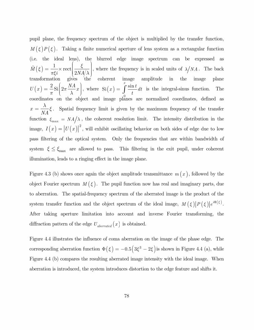
78
pupil plane, the frequency spectrum of the object is multiplied by the transfer function,
( ) ( )M Px x . Taking a finite numerical aperture of lens system as a rectangular function
(i.e. the ideal lens), the blurred edge image spectrum can be expressed as
( ) 1rect
2M
i NA
xx
px l
æ ö÷ç ÷ç= ´ ÷ç ÷ç ÷çè ø , where the frequency is in scaled units of NAl . The back
transformation gives the coherent image amplitude in the image plane
( ) 2Si 2
NAU x xp
p l
æ ö÷ç= ÷ç ÷÷çè ø, where ( )
0
sinSi
xt
x dtt
= ò is the integral-sinus function. The
coordinates on the object and image planes are normalized coordinates, defined as
xNA
lx= . Spatial frequency limit is given by the maximum frequency of the transfer
function max NAx l= , the coherent resolution limit. The intensity distribution in the
image, ( ) ( ) 2I x U x= , will exhibit oscillating behavior on both sides of edge due to low
pass filtering of the optical system. Only the frequencies that are within bandwidth of
system maxx x£ are allowed to pass. This filtering in the exit pupil, under coherent
illumination, leads to a ringing effect in the image plane.
Figure 4.3 (b) shows once again the object amplitude transmittance ( )m x , followed by the
object Fourier spectrum ( )M x . The pupil function now has real and imaginary parts, due
to aberration. The spatial-frequency spectrum of the aberrated image is the product of the
system transfer function and the object spectrum of the ideal image, ( ) ( ) ( )iM P e xx x F .
After taking aperture limitation into account and inverse Fourier transforming, the
diffraction pattern of the edge ( )aberratedU x is obtained.
Figure 4.4 illustrates the influence of coma aberration on the image of the phase edge. The
corresponding aberration function ( ) ( )30.5 3 2x x xF = - - is shown in Figure 4.4 (a), while
Figure 4.4 (b) compares the resulting aberrated image intensity with the ideal image. When
aberration is introduced, the system introduces distortion to the edge feature and shifts it.
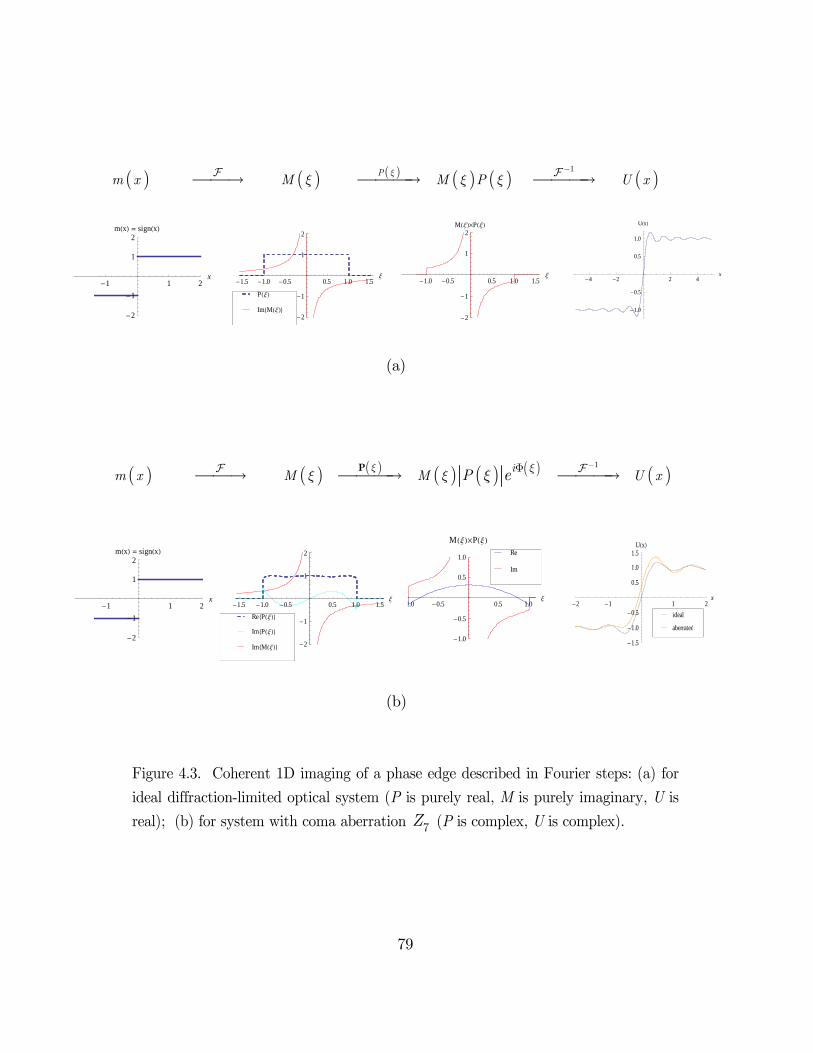
79
(a)
(b)
Figure 4.3. Coherent 1D imaging of a phase edge described in Fourier steps: (a) for
ideal diffraction-limited optical system (P is purely real, M is purely imaginary, U is
real); (b) for system with coma aberration 7Z (P is complex, U is complex).
-2 -1 1 2x
-1.5
-1.0
-0.5
0.5
1.0
1.5Ux
aberrated
ideal
-4 -2 2 4x
-1.0
-0.5
0.5
1.0
Ux
-1.5 -1.0 -0.5 0.5 1.0 1.5x
-2
-1
1
2
ImMxPx
-1 1 2x
-2
-1
1
2mx = signx
-1.0 -0.5 0.5 1.0 1.5x
-2
-1
1
2MxμPx
-1.0 -0.5 0.5 1.0x
-1.0
-0.5
0.5
1.0
MxμPx
Im
Re
-1 1 2x
-2
-1
1
2mx = signx
-1.5 -1.0 -0.5 0.5 1.0 1.5x
-2
-1
1
2
ImMxImPxRePx
( ) ( ) ( ) ( ) ( ) ( )1P
m x M M P U xx
x x x-
¾¾ ¾¾¾ ¾¾¾
( ) ( ) ( ) ( ) ( ) ( ) ( )1i
m x M M U xP ex xx x x
-F¾¾ ¾¾¾ ¾¾¾P
80
(a)
(b)
Figure 4.4. Phase edge with aberrations: (a) pupil phase function for the case
depicted in Figure 4.3b; (b) comparison of edge diffraction image intensities obtained
from the coherent image amplitudes obtained in Figure 4.3. The aberrated edge
centroid is shifted relative to the ideal position, according to PSF of a coma.
-2 -1 1 2x
0.5
1.0
1.5
Ix = UxUx
aberrated
ideal
-1.0 -0.5 0.5 1.0x
-1.0
-0.5
0.5
1.0Fx
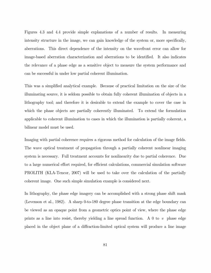
81
Figures 4.3 and 4.4 provide simple explanations of a number of results. In measuring
intensity structure in the image, we can gain knowledge of the system or, more specifically,
aberrations. This direct dependence of the intensity on the wavefront error can allow for
image-based aberration characterization and aberrations to be identified. It also indicates
the relevance of a phase edge as a sensitive object to measure the system performance and
can be successful in under low partial coherent illumination.
This was a simplified analytical example. Because of practical limitation on the size of the
illuminating source, it is seldom possible to obtain fully coherent illumination of objects in a
lithography tool; and therefore it is desirable to extend the example to cover the case in
which the phase objects are partially coherently illuminated. To extend the formulation
applicable to coherent illumination to cases in which the illumination is partially coherent, a
bilinear model must be used.
Imaging with partial coherence requires a rigorous method for calculation of the image fields.
The wave optical treatment of propagation through a partially coherent nonlinear imaging
system is necessary. Full treatment accounts for nonlinearity due to partial coherence. Due
to a large numerical effort required, for efficient calculations, commercial simulation software
PROLITH (KLA-Tencor, 2007) will be used to take over the calculation of the partially
coherent image. One such simple simulation example is considered next.
In lithography, the phase edge imagery can be accomplished with a strong phase shift mask
(Levenson et al., 1982). A sharp 0-to-180 degree phase transition at the edge boundary can
be viewed as an opaque point from a geometric optics point of view, where the phase edge
prints as a line into resist, thereby yielding a line spread function. A 0 to p phase edge
placed in the object plane of a diffraction-limited optical system will produce a line image
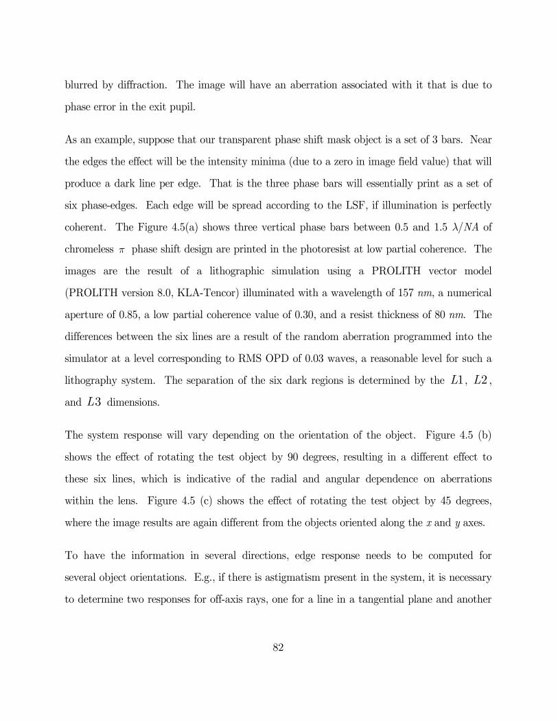
82
blurred by diffraction. The image will have an aberration associated with it that is due to
phase error in the exit pupil.
As an example, suppose that our transparent phase shift mask object is a set of 3 bars. Near
the edges the effect will be the intensity minima (due to a zero in image field value) that will
produce a dark line per edge. That is the three phase bars will essentially print as a set of
six phase-edges. Each edge will be spread according to the LSF, if illumination is perfectly
coherent. The Figure 4.5(a) shows three vertical phase bars between 0.5 and 1.5 l/NA of
chromeless p phase shift design are printed in the photoresist at low partial coherence. The
images are the result of a lithographic simulation using a PROLITH vector model
(PROLITH version 8.0, KLA-Tencor) illuminated with a wavelength of 157 nm, a numerical
aperture of 0.85, a low partial coherence value of 0.30, and a resist thickness of 80 nm. The
differences between the six lines are a result of the random aberration programmed into the
simulator at a level corresponding to RMS OPD of 0.03 waves, a reasonable level for such a
lithography system. The separation of the six dark regions is determined by the 1L , 2L ,
and 3L dimensions.
The system response will vary depending on the orientation of the object. Figure 4.5 (b)
shows the effect of rotating the test object by 90 degrees, resulting in a different effect to
these six lines, which is indicative of the radial and angular dependence on aberrations
within the lens. Figure 4.5 (c) shows the effect of rotating the test object by 45 degrees,
where the image results are again different from the objects oriented along the x and y axes.
To have the information in several directions, edge response needs to be computed for
several object orientations. E.g., if there is astigmatism present in the system, it is necessary
to determine two responses for off-axis rays, one for a line in a tangential plane and another
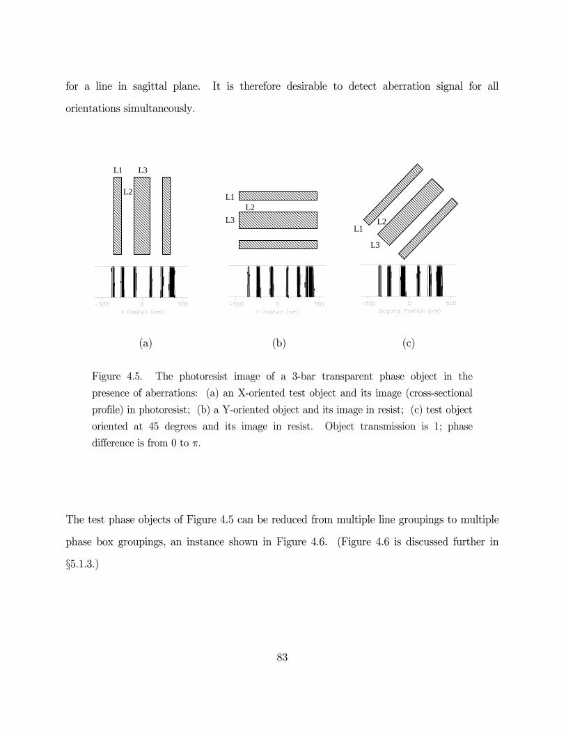
83
for a line in sagittal plane. It is therefore desirable to detect aberration signal for all
orientations simultaneously.
(a) (b) (c)
Figure 4.5. The photoresist image of a 3-bar transparent phase object in the
presence of aberrations: (a) an X-oriented test object and its image (cross-sectional
profile) in photoresist; (b) a Y-oriented object and its image in resist; (c) test object
oriented at 45 degrees and its image in resist. Object transmission is 1; phase
difference is from 0 to p.
The test phase objects of Figure 4.5 can be reduced from multiple line groupings to multiple
phase box groupings, an instance shown in Figure 4.6. (Figure 4.6 is discussed further in
§5.1.3.)
L1
L2
L3
L1L2
L3L1
L2
L3
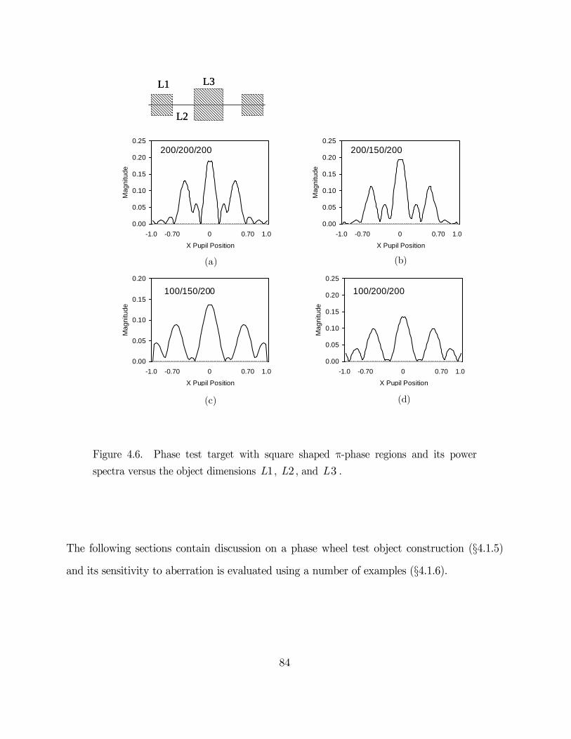
84
Figure 4.6. Phase test target with square shaped p-phase regions and its power
spectra versus the object dimensions 1L , 2L , and 3L .
The following sections contain discussion on a phase wheel test object construction (§4.1.5)
and its sensitivity to aberration is evaluated using a number of examples (§4.1.6).
0.00
0.05
0.10
0.15
0.20
0.25
X Pupil Position
Mag
nitu
de
-1.0 -0.70 0 0.70 1.0
0.00
0.05
0.10
0.15
0.20
0.25
X Pupil Position
Mag
nitu
de
-1.0 -0.70 0 0.70 1.0
0.00
0.05
0.10
0.15
0.20
0.25
X Pupil Position
Mag
nitu
de
-1.0 -0.70 0 0.70 1.0
0.00
0.05
0.10
0.15
0.20
0.25
X Pupil Position
Mag
nitu
de
-1.0 -0.70 0 0.70 1.0
0.00
0.05
0.10
0.15
0.20
X Pupil Position
Mag
nitu
de
-1.0 -0.70 0 0.70 1.0
0.00
0.05
0.10
0.15
0.20
X Pupil Position
Mag
nitu
de
-1.0 -0.70 0 0.70 1.0
0.00
0.05
0.10
0.15
0.20
0.25
X Pupil Position
Mag
nitu
de
-1.0 -0.70 0 0.70 1.0
0.00
0.05
0.10
0.15
0.20
0.25
X Pupil Position
Mag
nitu
de
-1.0 -0.70 0 0.70 1.0
L1
L2
L3L1
L2
L3
200/200/200 200/150/200
100/150/200 100/200/200
(b)(a)
(d)(c)
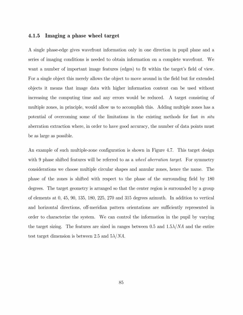
85
4.1.5 Imaging a phase wheel target
A single phase-edge gives wavefront information only in one direction in pupil plane and a
series of imaging conditions is needed to obtain information on a complete wavefront. We
want a number of important image features (edges) to fit within the target’s field of view.
For a single object this merely allows the object to move around in the field but for extended
objects it means that image data with higher information content can be used without
increasing the computing time and any errors would be reduced. A target consisting of
multiple zones, in principle, would allow us to accomplish this. Adding multiple zones has a
potential of overcoming some of the limitations in the existing methods for fast in situ
aberration extraction where, in order to have good accuracy, the number of data points must
be as large as possible.
An example of such multiple-zone configuration is shown in Figure 4.7. This target design
with 9 phase shifted features will be referred to as a wheel aberration target. For symmetry
considerations we choose multiple circular shapes and annular zones, hence the name. The
phase of the zones is shifted with respect to the phase of the surrounding field by 180
degrees. The target geometry is arranged so that the center region is surrounded by a group
of elements at 0, 45, 90, 135, 180, 225, 270 and 315 degrees azimuth. In addition to vertical
and horizontal directions, off-meridian pattern orientations are sufficiently represented in
order to characterize the system. We can control the information in the pupil by varying
the target sizing. The features are sized in ranges between 0.5 and 1.5l/NA and the entire
test target dimension is between 2.5 and 5l/NA.
86
Figure 4.7. Layout of a test target with multiple p-phase regions. Wheel aberration
target with 0°–180°, 90°–270°, 45°–225°, and 135°–315° azimuthal orientations.
Chromeless p phase shift design, i.e. the test target is a phase object where we have
variations in phase but not in amplitude.
The grouping of the features is not limited to the described example. The test structure can
also take on forms different than that shown in Figure 4.5 through Figure 4.7. Targets may
consist of various groupings of phase features of various sizing. The shape of the phase
features within the test target need not be square or circle. The shape of the features within
the target is less critical than the sizing and spacing since the detailed structure of the
features is likely beyond the resolution of the lithography system. The target in Figure 4.7
will produce similar intensity profiles along a central region of a multiple pattern grouping as
target in Figure 4.6. The transmission of the zones can be varied; the transmission of all
9045
0
315270
225
180
135
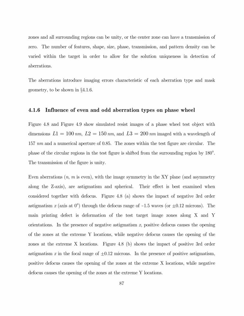
87
zones and all surrounding regions can be unity, or the center zone can have a transmission of
zero. The number of features, shape, size, phase, transmission, and pattern density can be
varied within the target in order to allow for the solution uniqueness in detection of
aberrations.
The aberrations introduce imaging errors characteristic of each aberration type and mask
geometry, to be shown in §4.1.6.
4.1.6 Influence of even and odd aberration types on phase wheel
Figure 4.8 and Figure 4.9 show simulated resist images of a phase wheel test object with
dimensions 1 100L = nm, 2 150L = nm, and 3 200L = nm imaged with a wavelength of
157 nm and a numerical aperture of 0.85. The zones within the test figure are circular. The
phase of the circular regions in the test figure is shifted from the surrounding region by 180.
The transmission of the figure is unity.
Even aberrations (n, m is even), with the image symmetry in the XY plane (and asymmetry
along the Z-axis), are astigmatism and spherical. Their effect is best examined when
considered together with defocus. Figure 4.8 (a) shows the impact of negative 3rd order
astigmatism x (axis at 0) through the defocus range of ~1.5 waves (or ±0.12 microns). The
main printing defect is deformation of the test target image zones along X and Y
orientations. In the presence of negative astigmatism x, positive defocus causes the opening
of the zones at the extreme Y locations, while negative defocus causes the opening of the
zones at the extreme X locations. Figure 4.8 (b) shows the impact of positive 3rd order
astigmatism x in the focal range of ±0.12 microns. In the presence of positive astigmatism,
positive defocus causes the opening of the zones at the extreme X locations, while negative
defocus causes the opening of the zones at the extreme Y locations.
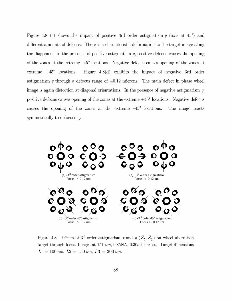
88
Figure 4.8 (c) shows the impact of positive 3rd order astigmatism y (axis at 45) and
different amounts of defocus. There is a characteristic deformation to the target image along
the diagonals. In the presence of positive astigmatism y, positive defocus causes the opening
of the zones at the extreme –45 locations. Negative defocus causes opening of the zones at
extreme +45 locations. Figure 4.8(d) exhibits the impact of negative 3rd order
astigmatism y through a defocus range of ±0.12 microns. The main defect in phase wheel
image is again distortion at diagonal orientations. In the presence of negative astigmatism y,
positive defocus causes opening of the zones at the extreme +45 locations. Negative defocus
causes the opening of the zones at the extreme –45 locations. The image reacts
symmetrically to defocusing.
Figure 4.8. Effects of 3rd order astigmatism x and y ( 5Z , 6Z ) on wheel aberration
target through focus. Images at 157 nm, 0.85NA, 0.30s in resist. Target dimensions
1 100L = nm, 2 150L = nm, 3 200L = nm.
(a) -3rd order astigmatism Focus +/- 0.12 um
(b) +3rd order astigmatism Focus +/- 0.12 um
(c) +3rd order 45° astigmatism Focus +/- 0.12 um
(d) -3rd order 45° astigmatism Focus +/- 0.12 um
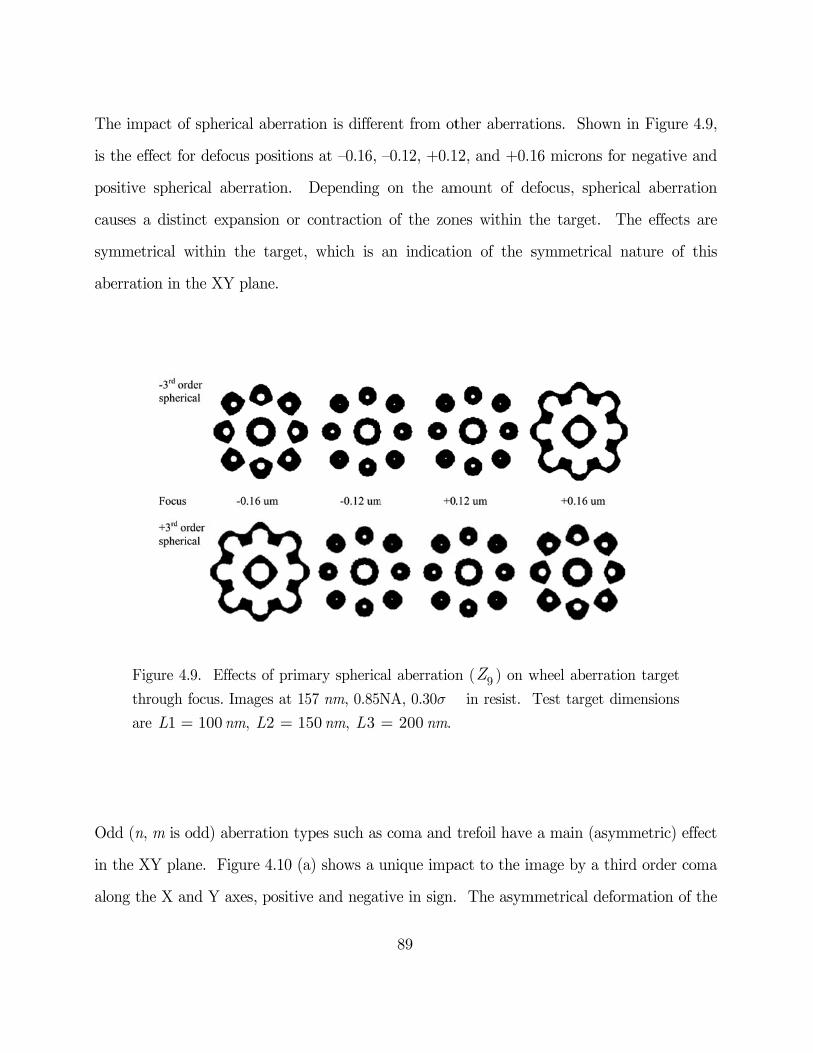
The imp
is the eff
positive
causes a
symmetr
aberratio
Fig
thro
are
Odd (n,
in the XY
along the
act of spher
fect for defo
spherical ab
distinct ex
rical within
on in the XY
gure 4.9. Eff
ough focus.
1 100L = n
m is odd) a
Y plane. Fi
e X and Y a
rical aberrat
cus position
berration.
xpansion or
the target
Y plane.
ffects of prim
Images at 1
nm, 2 1L =
berration ty
igure 4.10 (a
axes, positiv
tion is differ
ns at –0.16,
Depending
contraction
, which is
mary spheric
57 nm, 0.85N
150 nm, 3L
ypes such as
a) shows a u
ve and negat
89
rent from ot
–0.12, +0.1
on the am
n of the zon
an indicatio
al aberration
NA, 0.30s �
200= nm.
s coma and
unique impa
tive in sign.
ther aberrat
12, and +0.1
mount of de
nes within t
on of the s
n ( 9Z ) on w
in resist. T
trefoil have
act to the im
The asym
tions. Show
16 microns f
efocus, sphe
the target.
symmetrical
wheel aberra
Test target
a main (asy
mage by a t
mmetrical de
wn in Figure
for negative
erical aberra
The effects
l nature of
ation target
dimensions
ymmetric) e
third order c
formation o
e 4.9,
e and
ation
s are
f this
effect
coma
of the

90
image of the test target is seen for all orientations. The direction of vectors connecting
centers of inner and outer rings can be used as visual indicators of the aberration under
study. For each individual ring, a vector connecting the centers of inner and outer
boundary, can be used as indicator of deformation. The combination of all nine vectors can
be uniquely connected to the type of aberration present. Coma aberration results in image
where zones are opened and oriented toward a point, much like the familiar ray intersection
patterns (ray spot diagrams) for coma. The outermost zone along the direction of the coma
aberration, and opposite in sign, remains closed.
Figure 4.10 (b) shows the impact of the trefoil aberration x and y ( 10Z , 11Z ). The test
structures respond uniquely in all orientations. Trefoil aberration leaves the zones that are
opened and oriented toward a point. Unlike the coma aberration effects, the influence of
trefoil is a deformation of all zones and a convergence of vectors corresponding to a 120
degree symmetry of the aberration.
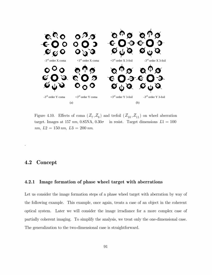
91
Figure 4.10. Effects of coma ( 7Z , 8Z ) and trefoil ( 10Z , 11Z ) on wheel aberration
target. Images at 157 nm, 0.85NA, 0.30s �in resist. Target dimensions 1 100L =nm, 2 150L = nm, 3 200L = nm.
.
4.2 Concept
4.2.1 Image formation of phase wheel target with aberrations
Let us consider the image formation steps of a phase wheel target with aberration by way of
the following example. This example, once again, treats a case of an object in the coherent
optical system. Later we will consider the image irradiance for a more complex case of
partially coherent imaging. To simplify the analysis, we treat only the one-dimensional case.
The generalization to the two-dimensional case is straightforward.
-3rd order X coma +3rd order X coma+3rd order X 3-foil -3rd order X 3-foil
-3rd order X coma +3rd order X coma
-3rd order Y coma +3rd order Y coma
+3rd order X 3-foil -3rd order X 3-foil
+3rd order Y 3-foil -3rd order Y 3-foil
(a) (b)
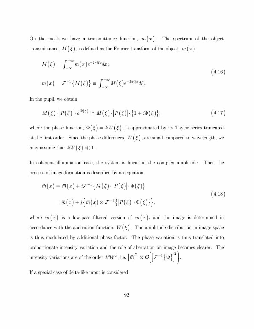
92
On the mask we have a transmittance function, ( )m x . The spectrum of the object
transmittance, ( )M x , is defined as the Fourier transform of the object, ( )m x :
In the pupil, we obtain
where the phase function, ( ) ( )kWx xF = , is approximated by its Taylor series truncated
at the first order. Since the phase differences, ( )W x , are small compared to wavelength, we
may assume that ( ) 1kW x .
In coherent illumination case, the system is linear in the complex amplitude. Then the
process of image formation is described by an equation
where ( )m x is a low-pass filtered version of ( )m x , and the image is determined in
accordance with the aberration function, ( )W x . The amplitude distribution in image space
is thus modulated by additional phase factor. The phase variation is thus translated into
proportionate intensity variation and the role of aberration on image becomes clearer. The
intensity variations are of the order 2 2k W , i.e. { }22 1m -æ öé ù ÷çµ F ÷ç ê ú ÷ç ë ûè ø
.
If a special case of delta-like input is considered
( )4.17( ) ( ) ( ) ( ) ( ) ( ){ }1 ,iM P e M P ixx x x x xF⋅ ⋅ @ ⋅ ⋅ + F
( )4.16
( ) ( )
( ) ( ){ } ( )
2
1 2
;
.
i x
i x
M m x e dx
m x M M e d
p x
p x
x
x x x
+¥ -
-¥
+¥- +-¥
=
= º
ò
ò
( )4.18
( ) ( ) ( ) ( ) ( ){ }
( ) ( ) ( ) ( ){ }{ }
1
1 ,
m x m x i M P
m x i m x P
x x x
x x
-
-
= + ⋅ ⋅ F
= + Ä ⋅ F

93
then ( )M x is equal to unity and the resulting field distribution in image is given by
Up to the first order in ( )kW x , we obtained the image that consists of a dominating real
part given by diffraction PSF, ( )h x , and an imaginary part, the disturbance given by the
Fourier inverse of the phase, ( )xF . The first term, ( )h x , is the unaberrated PSF, and the
second term is purely associated with aberration (as will be shown in Figure 4.12, middle
row).
The image, additionally superposed by a pattern due to phase part of the pupil, thus
becomes a sum of two terms. This introduces a linear phase factor in the complex amplitude
of the PSF, which is not present in the aberration-free PSF, and aberration gives rise to a
complex amplitude in image. The inverse Fourier transform is the difference between ideal
and aberrated PSF before it is multiplied by its complex conjugate (squared). The intensity
is proportional to h h* . Field signal is therefore proportional to pupil aberration and the
phase function can be made visible. The resulting wafer image intensity (squared modulus)
will show a difference between unaberrated and aberrated system PSFs.
It is clear from our simple analysis that the distortion caused by inclusion of aberration
presents itself in the shape proportional to the IFT of the wavefront itself. It has been
shown that the IFT’s of specific Zernikes are orthogonal (Dai, 2006) in space domain, and
therefore we can study the impact of each individual aberration term to understand the
impact of an arbitrary wavefront.
( )4.19( ) ( ),m x xd=
( )4.20
( ) ( ) ( ) ( ){ }
( ) ( ) ( ) ( ){ }
1
1
;
.aberrated ideal
m x h x i P
h x h x i P
x x
x x
-
-
= + ⋅ F
= + ⋅ F
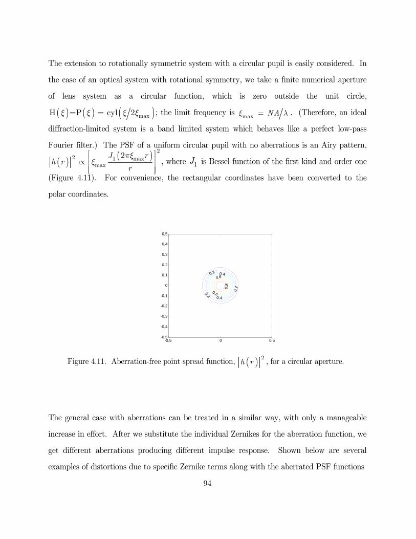
94
The extension to rotationally symmetric system with a circular pupil is easily considered. In
the case of an optical system with rotational symmetry, we take a finite numerical aperture
of lens system as a circular function, which is zero outside the unit circle, ( ) ( ) ( )maxH =P cyl 2x x x x= ; the limit frequency is
max NAx l= . (Therefore, an ideal
diffraction-limited system is a band limited system which behaves like a perfect low-pass
Fourier filter.) The PSF of a uniform circular pupil with no aberrations is an Airy pattern,
( ) ( ) 22 1 max
max
2J rh r
r
pxx
é ùê úµ ê úê úë û
, where 1J is Bessel function of the first kind and order one
(Figure 4.11). For convenience, the rectangular coordinates have been converted to the
polar coordinates.
Figure 4.11. Aberration-free point spread function, ( ) 2h r , for a circular aperture.
The general case with aberrations can be treated in a similar way, with only a manageable
increase in effort. After we substitute the individual Zernikes for the aberration function, we
get different aberrations producing different impulse response. Shown below are several
examples of distortions due to specific Zernike terms along with the aberrated PSF functions
0.2
0.2
0.2
0.4
0.4
0.6
0.6
0.8
-0.5 0 0.5-0.5
-0.4
-0.3
-0.2
-0.1
0
0.1
0.2
0.3
0.4
0.5
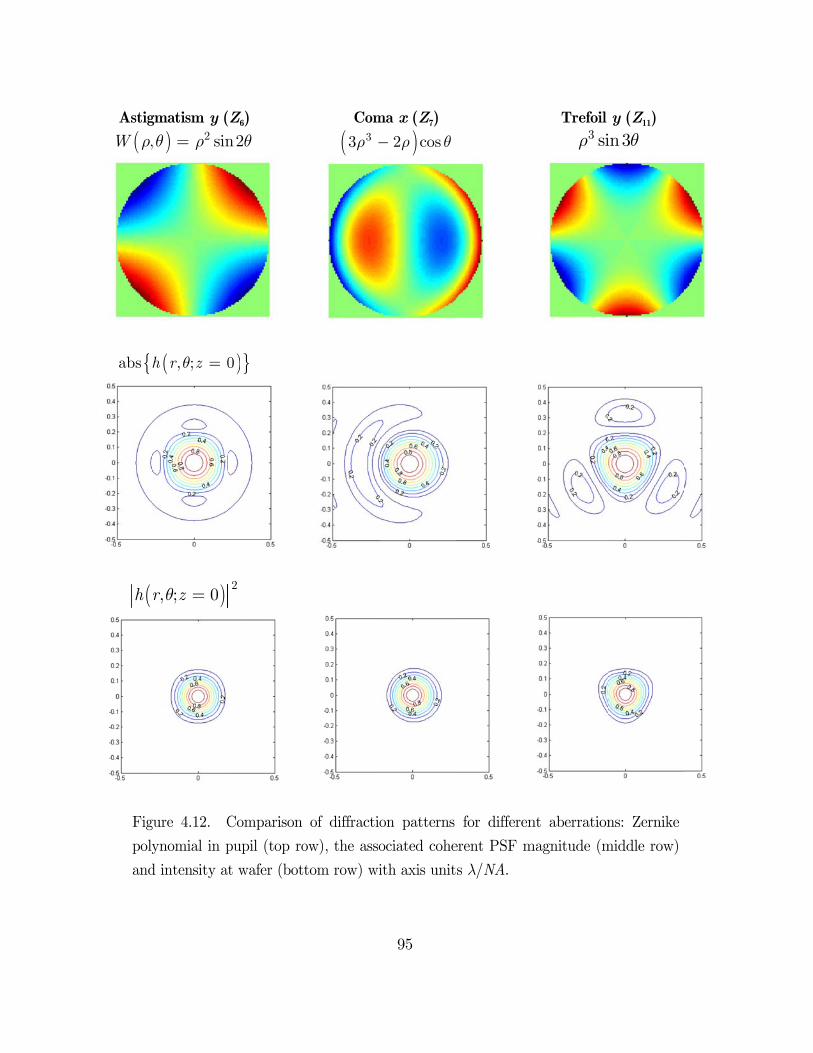
Astig
( ,W r
{abs
(h
Fig
poly
and
gmatism y (
) 2, sinq r=
( , ; 0h r zq =
), ; 0r zq =
gure 4.12. C
ynomial in p
d intensity at
Z6)
n2q
)}0
2
Comparison
pupil (top ro
t wafer (bott
Com
( 33r -
of diffractio
ow), the asso
tom row) wi
95
ma x (Z7)
)2 cosr q-
on patterns
ociated cohe
ith axis unit
for differen
erent PSF m
s l/NA.
Trefoil 3 sir
nt aberration
magnitude (m
y (Z11)
in3q
ns: Zernike
middle row)
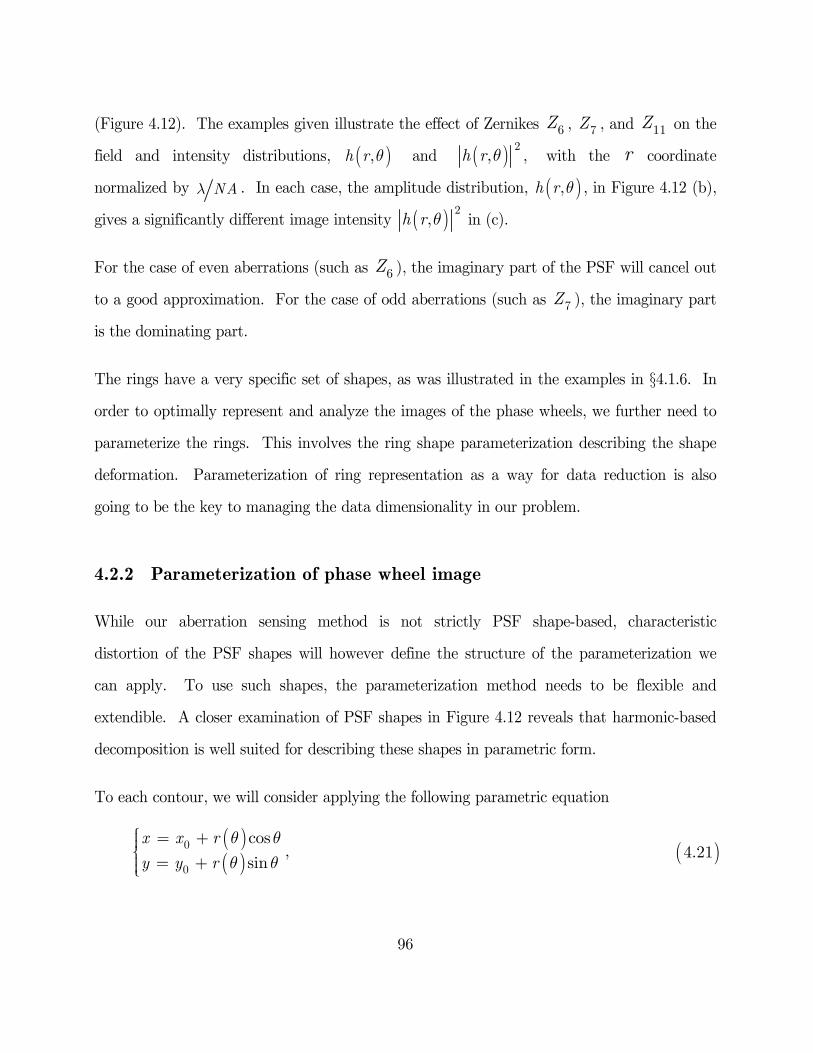
96
(Figure 4.12). The examples given illustrate the effect of Zernikes 6Z , 7Z , and 11Z on the
field and intensity distributions, ( ),h r q and ( ) 2,h r q , with the r
coordinate
normalized by NAl . In each case, the amplitude distribution, ( ),h r q , in Figure 4.12 (b),
gives a significantly different image intensity ( ) 2,h r q in (c).
For the case of even aberrations (such as 6Z ), the imaginary part of the PSF will cancel out
to a good approximation. For the case of odd aberrations (such as 7Z ), the imaginary part
is the dominating part.
The rings have a very specific set of shapes, as was illustrated in the examples in §4.1.6. In
order to optimally represent and analyze the images of the phase wheels, we further need to
parameterize the rings. This involves the ring shape parameterization describing the shape
deformation. Parameterization of ring representation as a way for data reduction is also
going to be the key to managing the data dimensionality in our problem.
4.2.2 Parameterization of phase wheel image
While our aberration sensing method is not strictly PSF shape-based, characteristic
distortion of the PSF shapes will however define the structure of the parameterization we
can apply. To use such shapes, the parameterization method needs to be flexible and
extendible. A closer examination of PSF shapes in Figure 4.12 reveals that harmonic-based
decomposition is well suited for describing these shapes in parametric form.
To each contour, we will consider applying the following parametric equation
( )4.21( )( )
0
0
cos,
sin
x x r
y y r
q qq q
ì = +ïïíï = +ïî
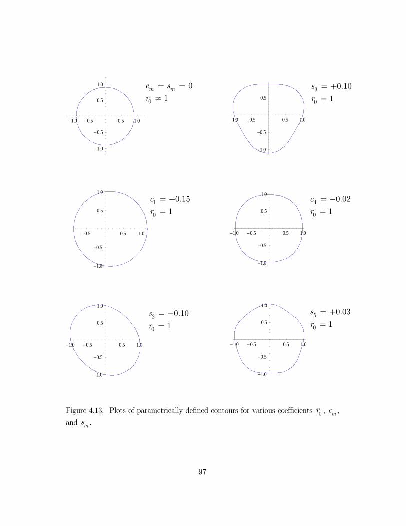
97
Figure 4.13. Plots of parametrically defined contours for various coefficients 0r , mc ,
and ms .
-1.0 -0.5 0.5 1.0
-1.0
-0.5
0.5
1.0
-0.5 0.5 1.0
-1.0
-0.5
0.5
1.0
-1.0 -0.5 0.5 1.0
-1.0
-0.5
0.5
1.0
-1.0 -0.5 0.5 1.0
-1.0
-0.5
0.5
-1.0 -0.5 0.5 1.0
-1.0
-0.5
0.5
1.0
-1.0 -0.5 0.5 1.0
-1.0
-0.5
0.5
1.0
0
0
1m mc s
r
= =¹
1
0
0.15
1
c
r
= +=
2
0
0.10
1
s
r
= -=
3
0
0.10
1
s
r
= +=
4
0
0.02
1
c
r
= -=
5
0
0.03
1
s
r
= +=
98
where
In Figure 4.13, examples of contours are given for different ring coefficients. The first one
corresponds to original circular shape, whose r coordinate does not depend on q . Other
plots show various shapes due to single non-zero parameters, mc or ms .
By this simple transformation, we can take the collection of ,x y ring contour points and
turn it into a parameterized description in polar coordinates with up to 13 parameters, for
each of the 18 rings in the target. Essentially, this is a coordinate transformation as well,
going from Cartesian to polar space. If radius is constant then only 3 parameters are
required and the ring is a perfect circle, these are the radius, 0r , and the center coordinates,
0 0,x y , of that ring.
Therefore, a ring shape can be compactly represented by a few (as few as 13) nonzero
coefficients. This form also allows us to decrease or increase the sample density accuracy of
the image.
4.2.3 Synthetic phase wheel images
The procedure of obtaining “synthetic” or simulated rings involves precisely modeling the
propagation of light from target to the detector in an image-forming system, and
subsequently measuring the simulated images. In lithography, the image measurements may
be derived either from the image intensity or from the image in photoresist. The Figure 4.14
( ) ( )
()
0 01
0 1 2 3 4 5
1 2 3 4 5
cos sin
1 cos cos2 cos 3 + cos 4 cos5
sin sin2 sin 3 sin 4 sin5 .
m mm
r r r c m s m
r c c c c c
s s s s s
q q q
q q q q q
q q q q q
=
= + +
= + + + +
+ + + + + +
å
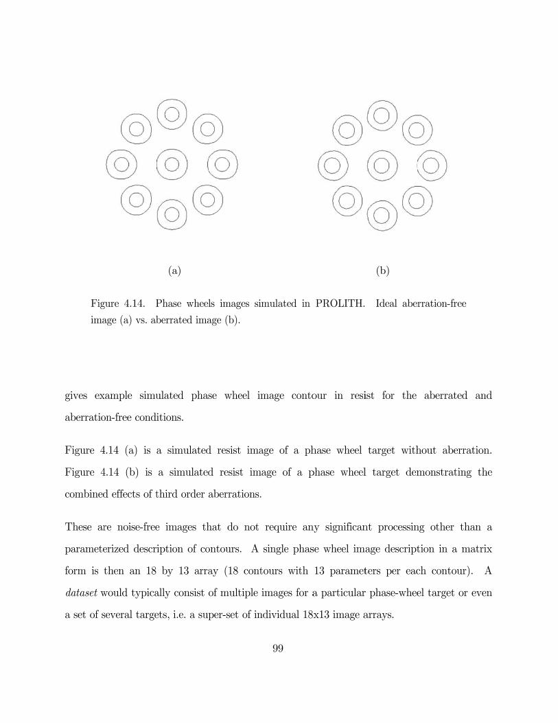
Fig
ima
gives ex
aberratio
Figure 4
Figure 4
combined
These ar
paramete
form is t
dataset w
a set of s
gure 4.14. P
age (a) vs. ab
xample simu
on-free cond
4.14 (a) is
4.14 (b) is
d effects of t
re noise-free
erized descr
then an 18
would typica
several targe
(a)
Phase wheel
berrated ima
ulated phas
itions.
a simulated
a simulated
third order a
e images th
iption of co
by 13 arra
ally consist o
ets, i.e. a sup
ls images si
age (b).
se wheel im
d resist ima
d resist im
aberrations.
hat do not
ontours. A
ay (18 cont
of multiple
per-set of in
99
mulated in
mage conto
age of a ph
mage of a p
.
require an
single phas
tours with
images for a
ndividual 18
PROLITH.
our in resi
hase wheel
phase wheel
ny significan
se wheel ima
13 paramet
a particular
x13 image a
(b)
Ideal aber
ist for the
target with
l target dem
nt processin
age descript
ters per eac
r phase-whee
arrays.
rration-free
aberrated
hout aberra
monstrating
ng other th
tion in a m
ch contour)
el target or
and
ation.
g the
han a
matrix
. A
even
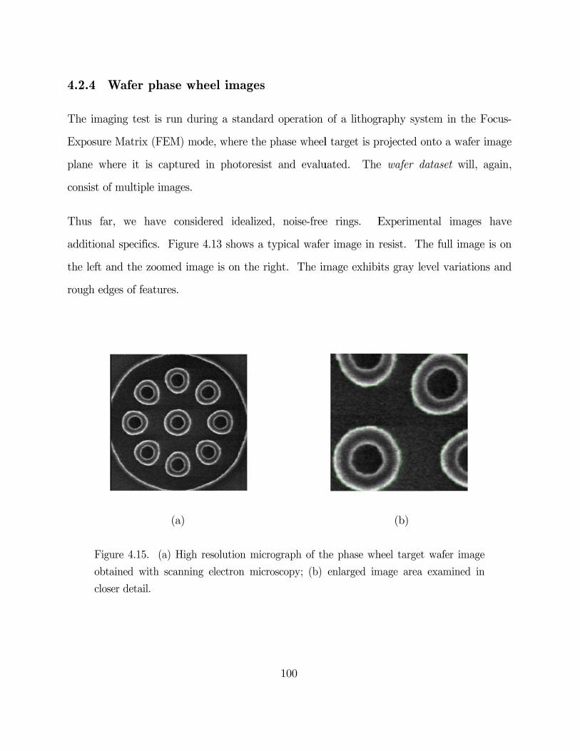
4.2.4 W
The ima
Exposure
plane wh
consist o
Thus fa
additiona
the left a
rough ed
Fig
obt
clos
Wafer ph
ging test is
e Matrix (F
here it is c
f multiple im
r, we have
al specifics.
and the zoom
dges of featu
gure 4.15. (a
tained with
ser detail.
hase wheel
run during
EM) mode,
captured in
mages.
e considere
Figure 4.13
med image
res.
(a)
a) High reso
scanning ele
l images
g a standard
where the p
photoresist
ed idealized
3 shows a t
is on the rig
olution micro
ectron micro
100
d operation
phase wheel
t and evalu
d, noise-free
ypical wafer
ght. The im
ograph of th
oscopy; (b)
of a lithogr
l target is pr
uated. The
e rings. E
r image in r
mage exhibi
he phase wh
enlarged im
raphy system
rojected ont
e wafer dat
Experimenta
resist. The
its gray leve
(b)
heel target w
mage area ex
m in the Fo
to a wafer im
aset will, a
al images
full image
el variations
wafer image
xamined in
ocus-
mage
again,
have
is on
s and
101
4.3 Analysis of experimental wafer image data
There are additional digital processing tasks that must be performed when dealing with
experimental resist images compared to the synthetic images. The high resolution wafer
images are obtained via the scanning electron microscopy (SEM). The origin of such images
is the scattered electron signal of low energies as collected by a detector. Low e-beam energy
is used to minimize charging of photoresist substrate but inevitably result in low image
contrast and low signal-to-noise ratio. SEM images typically show large variations in
brightness between different images, operating environments, and metrology equipment. We
anticipate the phase wheel edge regions to be significantly brighter than the other parts of
the SEM image due to higher density regions of back scattered electrons, however this object
delineation is not always clear cut. SEM usually has three or four different imaging modes.
In some cases the SEM image is already high-passed. Developing the computer code to
handle the extraction of resist edges is a necessary step to improve repeatability across
metrology tool sets by removing SEM algorithm influences from the aberration
measurement.
SEM image are typically 8-bit (256 gray levels) and at least 480x480 pixels in size or larger.
The field of view is on the order of 1 to 2 microns.
4.3.1 Image processing aspects
In order to be able to handle a large number of images in input data, we need to automate
the image and data processing. First, we need an automated way of segmenting the image
into regions and identifying ring objects in image, calculating the edge contour and ring
tracking. The typical steps requiring automation include: (1) image pre-processing (removal
of noise and edge roughness artifacts, low-level image processing operations); (2) edge

102
detection to help extract features within the target (image segmentation with edge-based
methods or thresholding, etc.), and (3) post processing (edge smoothing, pixel-to-physical
coordinate transformation, image registration, centering, scale and rotation).
Next, a description of different aspects of image segmentation will be given, namely:
A combination of methods that was considered to find local peak intensity and
thresholding; and morphological processing of images.
An optimization of wheel detection algorithm (Hough transform and active
contouring for edge detection).
The image segmentation stage required a lot of pre-processing and a number of digital image
processing techniques. See Gonzalez & Woods (2002) for an in-depth discussion on different
digital image processing concepts that have been considered. MATLAB® Image Processing
ToolboxTM environment was used for developing majority of the processing tasks (Gonzalez,
Woods, & Eddins, 2004). The papers by Li et al. (2005) and Tao et al. (2006) provide
implementation details on adapted algorithms, combination of which was found to give the
most reliable image segmentation result.
Image segmentation algorithms determine region boundaries in an image. We explored
several different approaches to image segmentation, including thresholding, edge-based
methods, and morphology-based methods. Some images at representative processing steps
are shown in Figure 4.16. The algorithms tested include: 1) the Canny method (see Figure
b, the Canny edge detection result); 2) thresholding of the original image (Figure c and
resulting edges highlighted around all elements in Figure d). The final result should look like
Figure e. Figure f also shows detail near the edge, exhibiting the edge roughness inherent in
resist imaging.
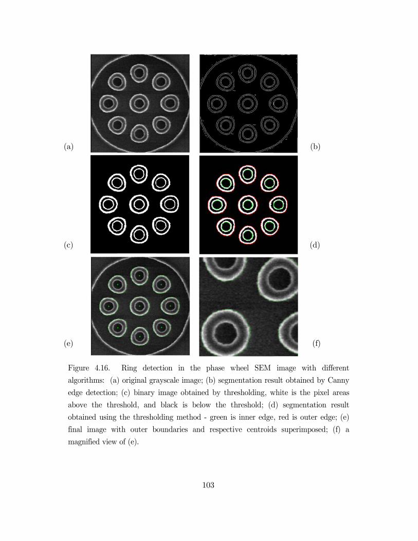
(a)
(c)
(e)
Fig
algo
edg
abo
obt
fina
ma
gure 4.16.
orithms: (a)
ge detection;
ove the thre
tained using
al image wi
gnified view
Ring dete
) original gra
(c) binary
eshold, and
the thresho
ith outer b
of (e).
ction in th
ayscale imag
image obtai
black is b
olding metho
oundaries a
103
he phase w
ge; (b) segm
ined by thre
below the th
od - green is
and respecti
wheel SEM
mentation res
esholding, w
hreshold; (d
s inner edge
ve centroid
(
(
image with
sult obtained
white is the
d) segmenta
, red is oute
s superimpo
(b)
d)
(f)
h different
d by Canny
pixel areas
ation result
er edge; (e)
osed; (f) a
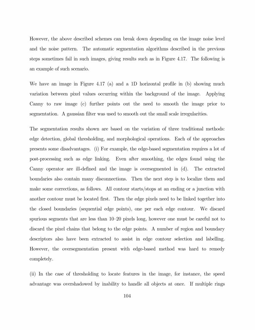
104
However, the above described schemes can break down depending on the image noise level
and the noise pattern. The automatic segmentation algorithms described in the previous
steps sometimes fail in such images, giving results such as in Figure 4.17. The following is
an example of such scenario.
We have an image in Figure 4.17 (a) and a 1D horizontal profile in (b) showing much
variation between pixel values occurring within the background of the image. Applying
Canny to raw image (c) further points out the need to smooth the image prior to
segmentation. A gaussian filter was used to smooth out the small scale irregularities.
The segmentation results shown are based on the variation of three traditional methods:
edge detection, global thresholding, and morphological operations. Each of the approaches
presents some disadvantages. (i) For example, the edge-based segmentation requires a lot of
post-processing such as edge linking. Even after smoothing, the edges found using the
Canny operator are ill-defined and the image is oversegmented in (d). The extracted
boundaries also contain many disconnections. Then the next step is to localize them and
make some corrections, as follows. All contour starts/stops at an ending or a junction with
another contour must be located first. Then the edge pixels need to be linked together into
the closed boundaries (sequential edge points), one per each edge contour. We discard
spurious segments that are less than 10–20 pixels long, however one must be careful not to
discard the pixel chains that belong to the edge points. A number of region and boundary
descriptors also have been extracted to assist in edge contour selection and labelling.
However, the oversegmentation present with edge-based method was hard to remedy
completely.
(ii) In the case of thresholding to locate features in the image, for instance, the speed
advantage was overshadowed by inability to handle all objects at once. If multiple rings

105
with different contrasts were present in the input pattern, it was difficult or impossible to
segment the desired features by thresholding alone. As can be seen in Figure (e), the circles
in the raw image have pixel gray scale differences along the edges, which could lead to faults
in local maxima detection. Here, the threshold properly locates the outer bright edges but
misses the fainter inner edges. If the threshold were set at a lower level to detect the fainter
edges, then the outer edges of some objects will be missed.
(iii) Figure 4.17 (f) shows the final result of a series of morphological operations applied to
input image for feature extraction, that result in some missing contours as well as partial
contour. A morphological approach works fairly well on good images yet some unpredictable
behavior is seen in (f), where one of rings will not be correctly identified. Groups of pixels
from two different edges are connected and identified as a single object. Figure (f) shows
how it will influence the final result.
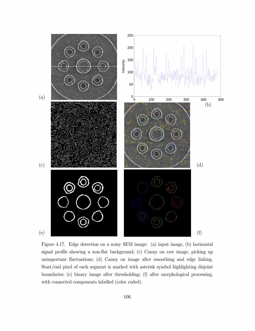
106
(a)
(b)
(c) (d)
(e) (f)
Figure 4.17. Edge detection on a noisy SEM image: (a) input image, (b) horizontal
signal profile showing a non-flat background; (c) Canny on raw image, picking up
unimportant fluctuations; (d) Canny on image after smoothing and edge linking.
Start/end pixel of each segment is marked with asterisk symbol highlighting disjoint
boundaries; (e) binary image after thresholding; (f) after morphological processing,
with connected components labelled (color coded).
0 100 200 300 400 5000
50
100
150
200
250
X
Inte
nsity

107
The examples shown in Figure 4.15 point out a number of weaknesses in the segmentation
approaches that worked reasonably well for the kind of image in Figure 4.13, which needed
to be addressed. The results were dramatically different on these two different kinds of
images.
The active contour approach was used for image segmentation in an effort to find a method
more robust to the presence of weak boundaries and strong noise. Active contours, or
snakes, are computer-generated spline curves (or active surfaces in 3D) that move within the
image to find object boundaries under the influence of internal and external forces by means
of energy minimization (Kass, Witkin, & Terzopoulos, 1987). The model applies the force on
the contour for it to evolve. A number of active contouring models exist that differ in their
implementation. Particular implementation followed here is that of Li et al. (2005), where
the active contour technique utilizes a zero level contour of a level set function defined in a
higher dimension, such as image gradient vector field, and evolves that function according to
a partial differential equation.
Due to a higher CPU load involved, the active contour algorithm can benefit from a proper
starting region. Minimum and maximum radii of the circles to be searched can provide
initial location for the active contour. The Hough transformation process was used to detect
circular shapes within the original grayscale image. Figure 4.18 (a) shows an image example
with the circles’ center positions and radii, as resolved by Hough transform. Main purpose of
computing the Hough projection is to produce 9 center locations (ignoring the radius or how
many rings) for the areas of interest. Binary mask obtained using circular Hough transform
result is used to initialize the active contour (Figure 4.18b).
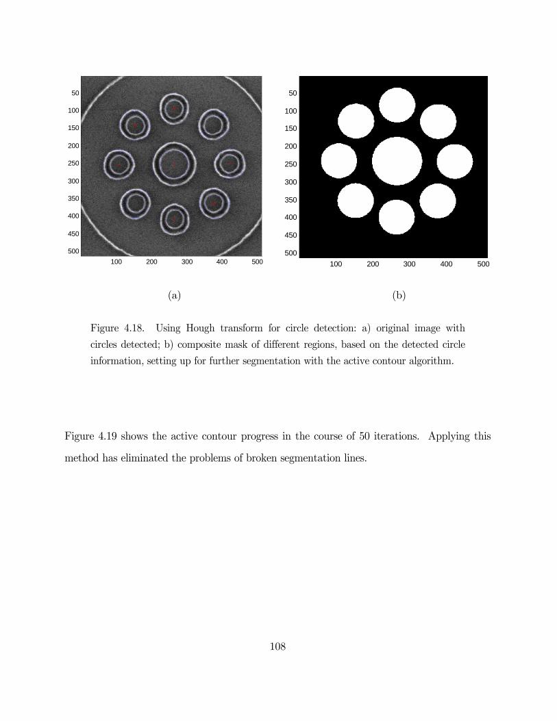
108
(a) (b)
Figure 4.18. Using Hough transform for circle detection: a) original image with
circles detected; b) composite mask of different regions, based on the detected circle
information, setting up for further segmentation with the active contour algorithm.
Figure 4.19 shows the active contour progress in the course of 50 iterations. Applying this
method has eliminated the problems of broken segmentation lines.
100 200 300 400 500
50
100
150
200
250
300
350
400
450
500
100 200 300 400 500
50
100
150
200
250
300
350
400
450
500
109
2 iterations 25 iterations
50 iterations
Figure 4.19. Segmentation result with active contour algorithm. Active contour
evolution of a center ring object in the course of 50 iterations.
50 100 150 200 250 300 350 400 450 500
50
100
150
200
250
300
350
400
450
500
50 100 150 200 250 300 350 400 450 500
50
100
150
200
250
300
350
400
450
500
50 100 150 200 250 300 350 400 450 500
50
100
150
200
250
300
350
400
450
500
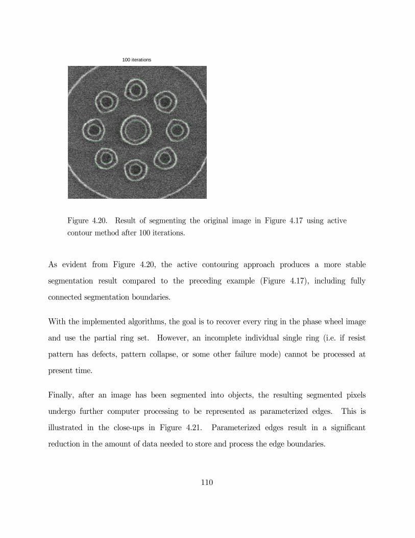
110
Figure 4.20. Result of segmenting the original image in Figure 4.17 using active
contour method after 100 iterations.
As evident from Figure 4.20, the active contouring approach produces a more stable
segmentation result compared to the preceding example (Figure 4.17), including fully
connected segmentation boundaries.
With the implemented algorithms, the goal is to recover every ring in the phase wheel image
and use the partial ring set. However, an incomplete individual single ring (i.e. if resist
pattern has defects, pattern collapse, or some other failure mode) cannot be processed at
present time.
Finally, after an image has been segmented into objects, the resulting segmented pixels
undergo further computer processing to be represented as parameterized edges. This is
illustrated in the close-ups in Figure 4.21. Parameterized edges result in a significant
reduction in the amount of data needed to store and process the edge boundaries.
100 iterations
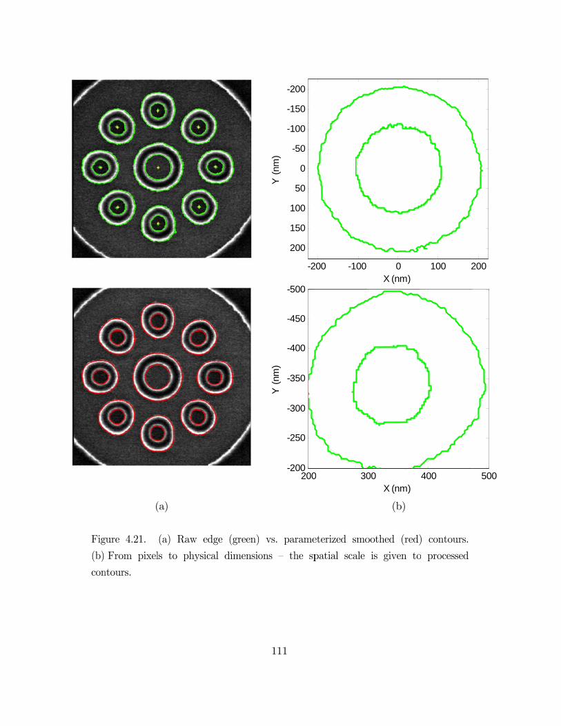
Fig
(b)
con
(
gure 4.21.
From pixel
ntours.
(a)
(a) Raw ed
ls to physic
dge (green)
cal dimensio
111
vs. parame
ons – the sp
-2
-200
-150
-100
-50
0
50
100
150
200
Y (
nm)
200
-500
-450
-400
-350
-300
-250
-200
Y (
nm)
eterized smo
patial scale
200 -100
0 30
(b)
oothed (red)
is given to
0X (nm)
00X (nm)
) contours.
o processed
100 2
400
200
500
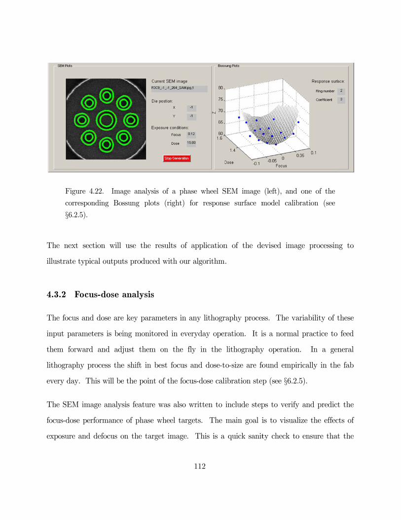
Fig
corr
§6.2
The nex
illustrate
4.3.2 F
The focu
input pa
them for
lithograp
every day
The SEM
focus-dos
exposure
gure 4.22. I
responding
2.5).
xt section w
e typical out
Focus-dos
us and dose
arameters is
rward and
phy process
y. This will
M image ana
se performan
and defocu
Image analy
Bossung pl
will use the
tputs produc
se analysi
are key par
being moni
adjust them
the shift in
l be the poin
alysis featur
nce of phas
us on the ta
ysis of a ph
lots (right)
e results of
ced with ou
is
rameters in
itored in ev
m on the
n best focus
nt of the foc
re was also
se wheel tar
arget image.
112
ase wheel S
for respons
application
r algorithm
any lithogr
veryday oper
fly in the
and dose-t
cus-dose cali
written to
rgets. The
. This is a
SEM image
se surface m
n of the de
.
raphy proces
ration. It i
lithography
o-size are fo
ibration step
include step
main goal i
quick sanit
(left), and
model calibr
evised imag
ss. The var
is a normal
y operation
ound empir
p (see §6.2.5
ps to verify
is to visuali
ty check to
one of the
ration (see
ge processin
riability of t
practice to
. In a ge
ically in the
5).
and predict
ize the effec
ensure that
ng to
these
feed
neral
e fab
t the
cts of
t the
113
images being fed into the system are being processed correctly. This is done by constructing
a family of curves, the so-called Bossung plots (Bossung, 1977).
Each SEM picture from Figure 4.23 is parameterized and analyzed as a function of exposure,
defocus, (and aberration), as demonstrated in Figure 4.25. The edges are extracted,
denoised, and superimposed over the SEM image. After performing image analysis, the
Focus-Exposure window of the phase wheel target parameters can be visualized, and used to
describe the edges in the test target (see §4.2.2), such as ring radius, width, etc.
Recall that each measured ring in a dataset is represented by 13 parameters that describe its
shape. Each coefficient in a dataset has a specific sensitivity to dose and focus as well as to
Zernike coefficients (to be discussed in Chapter 6). Visualizations, including familiar
Bossung-type plots help consolidate large amounts of information and facilitate the model
building process. Below is an example of such analysis.
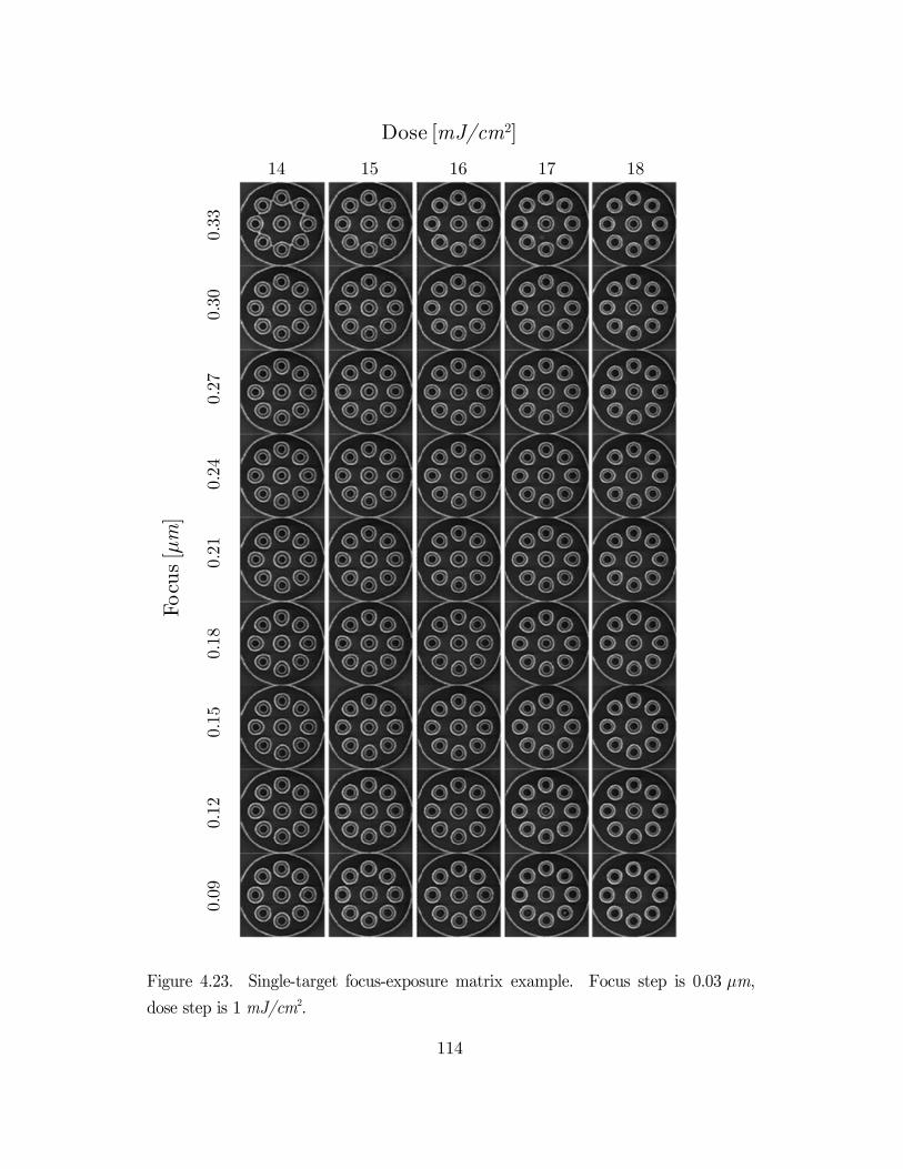
Fig
dos
Focu
s [μ
m]
gure 4.23. S
se step is 1 m
Focu
s [μ
m]
0.09
0.1
2
0.1
5
0.1
8
0.2
10.
24
0
.27
0.
30
0.
33
Single-target
mJ/cm2.
14
focus-expos
Dose
15
114
sure matrix
e [mJ/cm2
16
example. F
2]
17
Focus step i
18
is 0.03 μm,
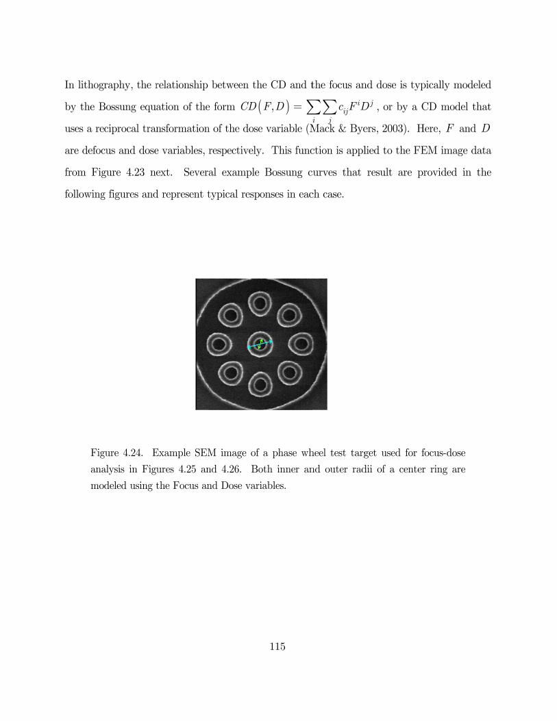
In lithogr
by the B
uses a re
are defoc
from Fig
following
Fig
ana
mo
raphy, the r
Bossung equ
ciprocal tran
cus and dose
gure 4.23 ne
g figures and
gure 4.24. E
alysis in Fig
deled using t
relationship
ation of the
nsformation
e variables,
ext. Sever
d represent t
Example SEM
ures 4.25 an
the Focus an
between th
e form (CD
n of the dose
respectively
al example
typical respo
M image of
nd 4.26. Bo
nd Dose vari
115
he CD and t
( ),i
F D = åe variable (M
y. This func
Bossung c
onses in eac
a phase wh
oth inner an
iables.
the focus an
iij
i j
c F DååMack & Bye
ction is appl
curves that
ch case.
heel test targ
nd outer rad
nd dose is ty
jD , or by a
ers, 2003).
lied to the F
result are
get used for
dii of a cent
ypically mod
a CD model
Here, F an
FEM image
provided in
r focus-dose
ter ring are
deled
that
nd D
data
n the
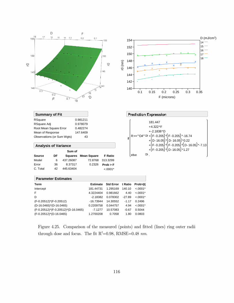
116
Figure 4.25. Comparison of the measured (points) and fitted (lines) ring outer radii
through dose and focus. The fit R2=0.98, RMSE=0.48 nm.
140
142
144
146
148
150
152
154
0.1 0.15 0.2 0.25 0.3 0.35
F (microns)
14
15
16
17
18
If
else
R=="'O4'"
181.447
+4.322*F
+-2.1838*D
+ F-0.205 * F-0.205 *-16.74
+ D-16.05 * D-16.05 *0.22
+ F-0.205 * F-0.205 * D-16.05 *-7.13
+ F-0.205 * D-16.05 *1.27
.
Intercept
F
D
(F-0.20512)*(F-0.20512)
(D-16.0465)*(D-16.0465)
(F-0.20512)*(F-0.20512)*(D-16.0465)
(F-0.20512)*(D-16.0465)
Term
181.44731
4.3224404
-2.18382
-16.73944
0.2209758
-7.1277
1.2700208
Estimate
1.295169
0.981662
0.078302
14.30552
0.044757
10.57083
0.7058
Std Error
140.10
4.40
-27.89
-1.17
4.94
-0.67
1.80
t Ratio
<.0001*
<.0001*
<.0001*
0.2496
<.0001*
0.5044
0.0803
Prob>|t|
Parameter Estimates
RSquare
RSquare Adj
Root Mean Square Error
Mean of Response
Observations (or Sum Wgts)
0.981211
0.978079
0.482274
147.6409
43
Summary of Fit
Model
Error
C. Total
Source
6
36
42
DF
437.26087
8.37317
445.63404
Sum of
Squares
72.8768
0.2326
Mean Square
313.3299
F Ratio
<.0001*
Prob > F
Analysis of Variance
D (mJ/cm2)
r0 (
nm)
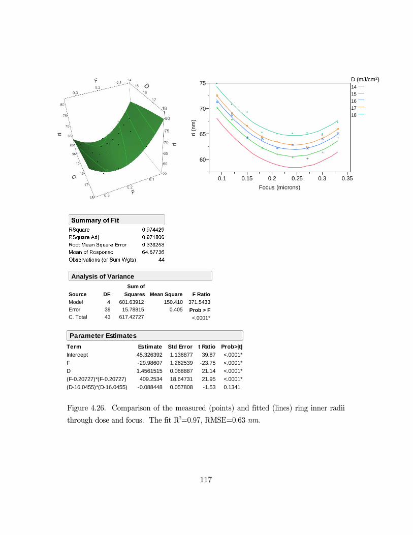
117
Figure 4.26. Comparison of the measured (points) and fitted (lines) ring inner radii
through dose and focus. The fit R2=0.97, RMSE=0.63 nm.
60
65
70
75
0.1 0.15 0.2 0.25 0.3 0.35
Focus (microns)
14
15
16
17
18
Intercept
F
D
(F-0.20727)*(F-0.20727)
(D-16.0455)*(D-16.0455)
Term
45.326392
-29.98607
1.4561515
409.2534
-0.088448
Estimate
1.136877
1.262539
0.068887
18.64731
0.057808
Std Error
39.87
-23.75
21.14
21.95
-1.53
t Ratio
<.0001*
<.0001*
<.0001*
<.0001*
0.1341
Prob>|t|
Parameter Estimates
Model
Error
C. Total
Source
4
39
43
DF
601.63912
15.78815
617.42727
Sum of
Squares
150.410
0.405
Mean Square
371.5433
F Ratio
<.0001*
Prob > F
Analysis of Variance
D (mJ/cm2)
ri(n
m)
ri
ri
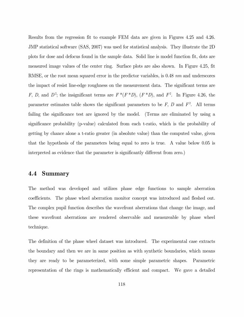
118
Results from the regression fit to example FEM data are given in Figures 4.25 and 4.26.
JMP statistical software (SAS, 2007) was used for statistical analysis. They illustrate the 2D
plots for dose and defocus found in the sample data. Solid line is model function fit, dots are
measured image values of the center ring. Surface plots are also shown. In Figure 4.25, fit
RMSE, or the root mean squared error in the predictor variables, is 0.48 nm and underscores
the impact of resist line-edge roughness on the measurement data. The significant terms are
F, D, and D 2; the insignificant terms are F *(F *D), (F *D), and F 2. In Figure 4.26, the
parameter estimates table shows the significant parameters to be F, D and F 2. All terms
failing the significance test are ignored by the model. (Terms are eliminated by using a
significance probability (p-value) calculated from each t-ratio, which is the probability of
getting by chance alone a t-ratio greater (in absolute value) than the computed value, given
that the hypothesis of the parameters being equal to zero is true. A value below 0.05 is
interpreted as evidence that the parameter is significantly different from zero.)
4.4 Summary
The method was developed and utilizes phase edge functions to sample aberration
coefficients. The phase wheel aberration monitor concept was introduced and fleshed out.
The complex pupil function describes the wavefront aberrations that change the image, and
these wavefront aberrations are rendered observable and measureable by phase wheel
technique.
The definition of the phase wheel dataset was introduced. The experimental case extracts
the boundary and then we are in same position as with synthetic boundaries, which means
they are ready to be parameterized, with some simple parametric shapes. Parametric
representation of the rings is mathematically efficient and compact. We gave a detailed
119
example in §4.2 regarding the use of those expressions. Parameterized edge description
presents a unified way to analyze the shape of any (synthetic and empirical) boundary. In
this way, a highly efficient, compressed representation is achieved.
Also discussed, in §4.3, is the analysis of wafer rings and the problem of segmenting regions
out of an image. A technique for automatic segmentation of a phase wheel image has been
developed. Segmentation is a challenging task, particularly with noisy images. It is sensitive
to LER present in resist image. If simple threshold or edge detection routines fail, more
sophisticated approaches are needed that work with low contrast SEM images of resist.
SEM image processing is a combination of active contour and Hough transform methods
resulting in a more reliable edge placement, making the SEM processing algorithms robust.
The active contour (aka the snake) algorithm is tuned for SEM images to allow detection of
borders between poorly distinguished image areas that contain similar pixel values. It
provides a high reliability in detecting edges of image objects. The analysis of SEM images
has been reduced to an automated procedure. The image processing and the related
algorithms were implemented in MATLAB. Operations shown in §4.3.1 demonstrate what is
possible with the written tool kit.

120
5. Phase wheel experimental testing
5.1 Approach
Following the concept testing phase in Chapter 4, this chapter examines the lithographic
experimental setup including: design and fabrication of test structures; target selection;
optimization; and print tests. In §5.2, two kinds of aberration extraction feasibility studies
were performed based on early experimental imaging tests and simulations. While §5.2.1
addresses methods for estimation from intensity image data and the error, §5.2.2 discusses
extensions of the method to the resist test.
The simulation study is described in §5.2.1; proof of concept is given. Model aliasing aspect
is briefly mentioned in §5.2.1, as well. Subsequently, the real experiment example of this is
given in §5.2.2, and §5.2.3 contains a summary of method and results discussion.
5.1.1 Aberration test implementation
Experimental implementation requires producing a varying intensity signal at the image
plane. The phase wheel target implementation is made possible through a standard phase
shift mask with chromeless p-phase shifted regions defining the test object structure in
121
complex amplitude. The shape of a target is etched into the reticle substrate. A 0/180°
phase-edge target provides maximum contrast at the wafer for resist as detector.
The image testing procedure is a standard operation of a lithography system where the
phase wheel target is projected onto a wafer image plane where it is captured in photoresist
and evaluated. The target is exposed at a single illumination setting (maximum NA and low
s) through focus and dose. Images of the pattern are formed in a thin layer of conventional,
high contrast resist with the scanner operating in a standard focus exposure matrix (FEM)
mode, where exposure dose and focus are changed by column and row. An SEM is used to
collect and store digitized images for use in the image processing step.
The aberration effects on the image are estimated by studying the image intensity changes
coupled with defocus. The main image is the in-focus image that has been degraded by the
unknown aberrations. Additional images of the same object are formed by perturbing these
aberrations with a known amount of phase error, such as defocus. The relative phase
difference introduced between the wavefronts is encoded within each corresponding image’s
signal.
Aberration analysis (see §5.2.2) is carried out through the use of lithography modeling, where
simulated images can be produced without aberration and with various levels of lens
aberrations. A lens aberration detection is based on the identification of deviations that
occur between images printed with a test target and images that would be produced in the
absence of aberrations. Printed resist images are compared to simulated resist images, while
coefficient values for primary Zernike aberrations are varied. (A more rigorous mathematical
analysis of images using a fitting algorithm is possible for aberration parameter fitting and
will be explored in Chapter 6.) For lenses with large aberrations, the detection of specific
122
aberration types and trends, as well as levels of aberrations, is possible though a visual
inspection due to the ease with which aberrations can be distinguished.
The extraction of aberration information is a critical step in this process because of the often
subtle shape deformation that is introduced into the ring images with small levels of
aberration. As covered in §4.3, such analysis needs to be robust and efficient.
The target dimensions, structures, orientations, and placement are optimized to
accommodate specific imaging conditions (l and NA). To optimize the parameters of
suitable test structures, an analysis is performed using a lithographic simulator for design
and layout.
5.1.2 Mask design
The phase wheel target object is implemented as a photomask which is fabricated using
methods that are common to phase-shift photomask fabrication. Transmission of the test
object is controlled through patterning of the masking layer. The routine steps involved in
the fabrication of the photomask include: (i) the layout of the test object using computer
aided design or other methods; (ii) exposing a sensitized polymer film coated over a quartz
plate which may also have a masking film; (iii) developing the exposed image; and (iv)
transferring the pattern onto the photomask using a dry or wet pattern transfer process.
The phase definition (the phase shift within the regions of the test object) is achieved
through etching of the quartz substrate to a depth corresponding to a 180° phase shift, with
possible depth correction incorporated to account for phase effects of the relief structure of
the mask.
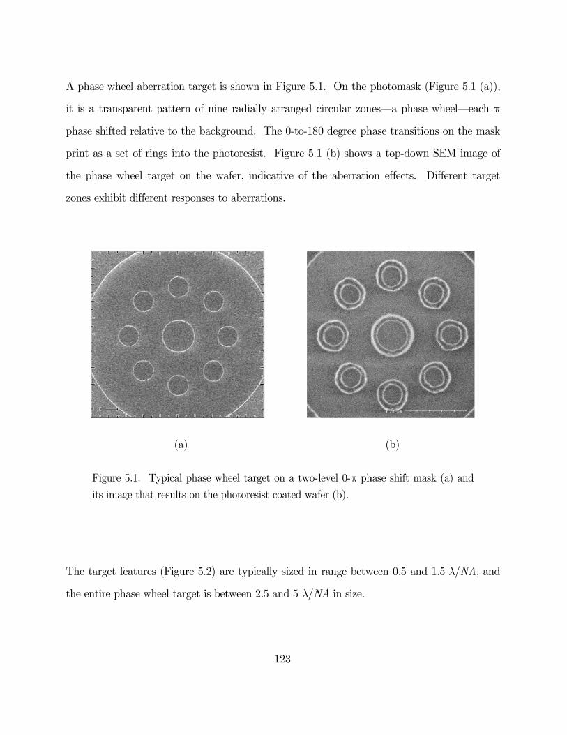
A phase
it is a tr
phase shi
print as
the phas
zones exh
Fig
its
The targ
the entir
wheel aberr
ransparent p
ifted relativ
a set of ring
se wheel tar
hibit differen
gure 5.1. Ty
image that r
get features
e phase whe
ration target
pattern of n
ve to the bac
gs into the
rget on the
nt responses
(a)
ypical phase
results on th
(Figure 5.2)
eel target is
t is shown i
nine radially
ckground. T
photoresist.
wafer, indi
s to aberrati
wheel targe
he photoresis
) are typica
between 2.5
123
in Figure 5.
y arranged c
The 0-to-180
. Figure 5.1
icative of th
ions.
et on a two-
t coated waf
ally sized in
5 and 5 l/N
1. On the p
circular zon
0 degree ph
1 (b) shows
he aberratio
level 0-p ph
fer (b).
range betw
NA in size.
photomask
nes—a phase
hase transitio
s a top-down
on effects.
(b)
hase shift ma
ween 0.5 and
(Figure 5.1
e wheel—ea
ons on the m
n SEM ima
Different ta
ask (a) and
d 1.5 l/NA,
(a)),
ach p
mask
age of
arget
, and
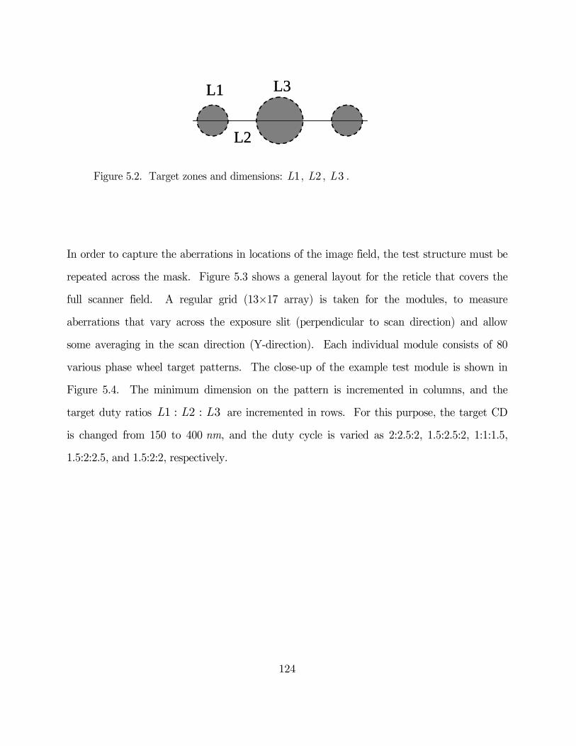
124
Figure 5.2. Target zones and dimensions: 1L , 2L , 3L .
In order to capture the aberrations in locations of the image field, the test structure must be
repeated across the mask. Figure 5.3 shows a general layout for the reticle that covers the
full scanner field. A regular grid (13×17 array) is taken for the modules, to measure
aberrations that vary across the exposure slit (perpendicular to scan direction) and allow
some averaging in the scan direction (Y-direction). Each individual module consists of 80
various phase wheel target patterns. The close-up of the example test module is shown in
Figure 5.4. The minimum dimension on the pattern is incremented in columns, and the
target duty ratios 1 : 2 : 3L L L are incremented in rows. For this purpose, the target CD
is changed from 150 to 400 nm, and the duty cycle is varied as 2:2.5:2, 1.5:2.5:2, 1:1:1.5,
1.5:2:2.5, and 1.5:2:2, respectively.
L1
L2
L3L1
L2
L3
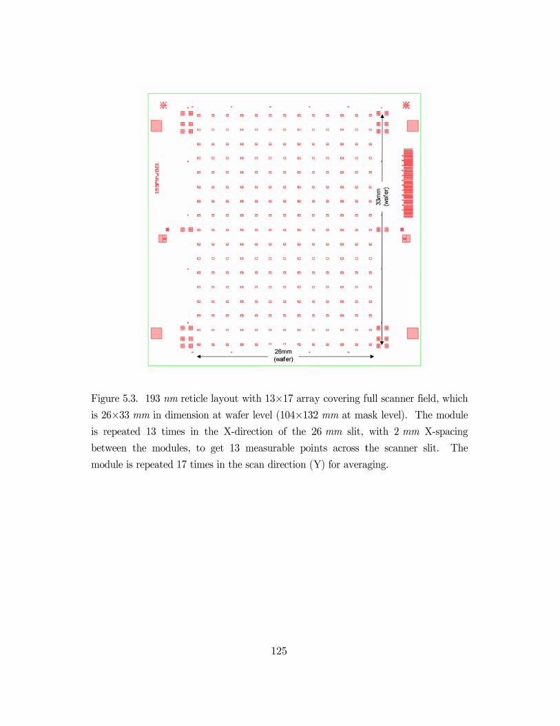
Fig
is 2
is r
bet
mo
gure 5.3. 193
26×33 mm in
repeated 13
ween the m
dule is repea
3 nm reticle
n dimension
times in th
modules, to
ated 17 time
layout with
at wafer lev
he X-directi
get 13 mea
s in the scan
125
13×17 arra
vel (104×132
ion of the 2
asurable poin
n direction (Y
ay covering f
2 mm at ma
26 mm slit,
nts across t
Y) for avera
full scanner f
ask level). T
with 2 mm
the scanner
aging.
field, which
The module
m X-spacing
slit. The
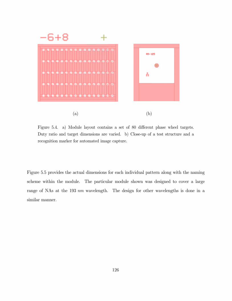
Fig
Dut
reco
Figure 5.
scheme w
range of
similar m
gure 5.4. a)
ty ratio and
ognition mar
.5 provides
within the
NAs at th
manner.
(a)
) Module la
d target dim
rker for auto
the actual d
module. T
he 193 nm w
ayout contai
mensions are
omated imag
dimensions f
The particul
wavelength.
126
ns a set of
varied. b)
ge capture.
for each ind
lar module
The desig
(b)
80 different
Close-up of
dividual patt
shown was
gn for other
t phase whe
a test struc
tern along w
s designed t
r wavelengt
eel targets.
cture and a
with the nam
to cover a
ths is done
ming
large
in a
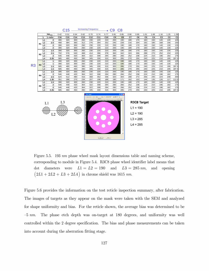
Fig
corr
dot
(2L
Figure 5.
The imag
for shape
–5 nm.
controlle
into acco
R
R
R
R
R
R3
gure 5.5. 19
responding t
t diameters
1 2 2L L+ +
.6 provides
ges of targe
e uniformity
The phase
d within the
ount during
NAmax 0
L L-ratio CL1 2 3L2 2.5 4L3 2 3L4 2 3
L1 1.5 3L2 2.5 7L3 2 5L4 2.25 5
L1 1 3L2 1 3L3 1.5 5L4 1.5 5
L1 1.5 3L2 2 5L3 2.5 6L4 1.35 3
L1 1.5 3L2 2 5L3 2 5L4 2.25 5
R5
R1
R2
R3
R4
3 nm phase
to module in
s were L
3 2 4L L+ +
the informa
ets as they a
y and bias.
e etch dept
e 2 degree s
the aberrat
.42 0.51 0.54
C16 C15 C14390 320 300468 384 360390 320 300390 320 300390 320 300702 576 540546 448 420585 480 450390 320 300390 320 300585 480 450585 480 450390 320 300546 448 420624 512 480351 288 270390 320 300546 448 420546 448 420585 480 450
C15 I
wheel mask
n Figure 5.4.
1 2L L= =
) in chrome
ation on the
appear on t
For the ret
th was on-t
specification
ion fitting s
0.62 0.70 0.
C13 C12 C260 230 2312 276 2260 230 2260 230 2260 230 2468 414 3364 322 3390 345 3260 230 2260 230 2390 345 3390 345 3260 230 2364 322 3416 368 3234 207 1260 230 2364 322 3364 322 3390 345 3
Increasing Frequency
127
k layout dim
R3C8 phas
190 and
e shield was
test reticle
the mask w
icle shown,
target at 1
n. The bias
stage.
.74 0.77 0.81
C11 C10 C9220 210 200264 252 240220 210 200220 210 200220 210 200396 378 360308 294 280330 315 300220 210 200220 210 200330 315 300330 315 300220 210 200308 294 280352 336 320198 189 180220 210 200308 294 280308 294 280330 315 300
C9y
mensions tabl
se wheel iden
3 28L = 1615 nm.
inspection
were taken w
the average
180 degrees,
and phase m
0.85 0.90 0.
C8 C7190 180 1228 216 2190 180 1190 180 1190 180 1342 324 3266 252 2285 270 2190 180 1190 180 1285 270 2285 270 2190 180 1266 252 2304 288 2171 162 1190 180 1266 252 2266 252 2285 270 2
C8
le and nami
ntifier label m
85 nm, and
summary, a
with the SEM
e bias was d
, and unifo
measuremen
95 1.01 1.08
C6 C5 C470 160 150
204 192 18070 160 15070 160 15070 160 150
306 288 270238 224 210255 240 22570 160 15070 160 150
255 240 225255 240 22570 160 150
238 224 210272 256 24053 144 13570 160 150
238 224 210238 224 210255 240 225
ng scheme,
means that
d opening
after fabrica
M and anal
determined t
ormity was
nts can be t
1.16 1.25 1.
C3 C2 C140 130 1168 156 1140 130 1140 130 1140 130 1252 234 2196 182 1210 195 187140 130 1140 130 1210 195 187210 195 187140 130 1196 182 1224 208 2126 117 112140 130 1196 182 1196 182 1210 195 187
ation.
lyzed
to be
well
taken
35
C125502525252575
7.52525
7.57.5257500
2.5257575
7.5
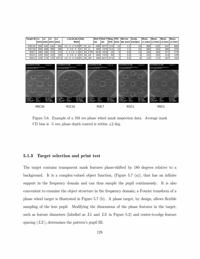
R
Fig
CD
5.1.3 T
The targ
backgrou
support
convenien
phase wh
sampling
such as f
spacing (
Target ID L(
R5C16:R1C16:
R3C7:R1C1:R5C1:
R5C16
gure 5.6. Ex
D bias is –5 n
Target se
get contains
und. It is a
in the frequ
nt to exami
heel target i
g of the lens
feature diam
( 2L ), deter
L1 (nm)
L2 (nm)
L3 (nm)
L(n
390 546 546390 468 390180 180 270125 150 125125 175 175
R1C16
xample of a 1
nm; phase de
lection an
s transparen
a complex-v
uency doma
ne the objec
is illustrated
s pupil. M
meters (labe
mines the p
L4 nm)
L1/L2/L3R
585 1.5 : 2 : 2: 2390 2 : 2.5 : 270 1 : 1: 1.5 125 2 : 2.5 :
187.5 1.5 : 2 : 2: 2
193 nm phas
epth control
nd print t
nt mask fea
valued objec
ain and can
ct structure
d in Figure
Modifying th
lled as 1L
pattern’s pup
3/L4 Ratio
Site
2.25 F1_S1_UL2 : 2 F1_S2_LL: 1.5 F1_S3_CTR2 : 2 F1_S4_LR2.25 F1_S5_UR
128
R3C7
se wheel ma
is within ±2
test
atures phase
ct function,
n thus samp
in the frequ
5.7 (b). A
he dimension
and 3L in
pil fill.
Waf X um
Waf Y um
Mag(kX)
-599 8277 12.-600 7475 12.39.8 7876 2600 7475 5600 8277 37.
R1C
ask inspection
2 deg.
e-shifted by
(Figure 5.7
ple the pup
uency doma
phase targe
ns of the ph
Figure 5.2)
g )
FOV (um)
Micron bar (um)
5 12 1.25 12 1.25 6 0.60 3 0.35 4 0.4
C1
n data. Ave
y 180 degre
7 (a)), that
pil continuo
ain; a Fourie
et, by design
hase feature
) and center
Scale (nm/pix)
Meas L1 (nm)
24 38524 38512 184
6 1158 115
R5C1
erage mask
ees relative
t has an inf
ously. It is
er transform
n, allows fle
es in the ta
r-to-edge fea
)Meas L2 (nm)
Meas L3 (nm)
5 522 5475 444 3854 183 2775 154 1135 172 167
to a
finite
also
m of a
exible
arget,
ature
)Meas L4 (nm)
7 5825 3757 2733 1207 181
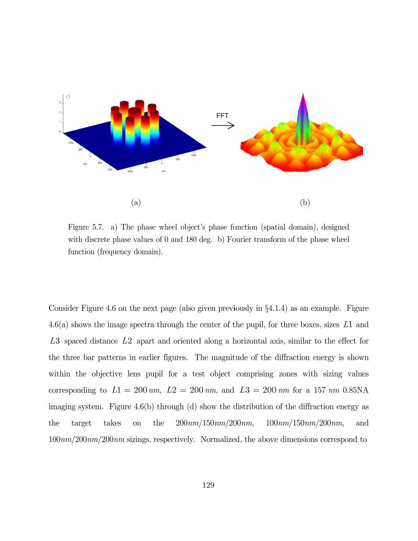
Fig
wit
fun
Consider
4.6(a) sh
3L spac
the three
within t
correspon
imaging
the ta
100nm/2
f
gure 5.7. a)
h discrete ph
nction (freque
r Figure 4.6
hows the ima
ced distance
e bar patter
the objectiv
nding to L
system. Fig
arget take
200nm/200n
(a)
The phase
hase values o
ency domain
on the next
age spectra
e 2L apart
rns in earlie
ve lens pup
1 200= nm
gure 4.6(b)
es on th
nm sizings, r
wheel objec
of 0 and 180
n).
t page (also
through the
and oriente
er figures. T
pil for a t
m, 2 20L =
through (d)
he 200nm
respectively.
129
ct’s phase fu
0 deg. b) Fo
given previ
e center of t
ed along a h
The magnit
est object
00 nm, and
) show the d
m/150nm/20
Normalize
FFT
unction (spa
ourier transfo
iously in §4.
the pupil, fo
horizontal a
tude of the
comprising
3 200L =
distribution
00nm, 10
ed, the abov
(b)
atial domain
orm of the p
.1.4) as an e
or three box
axis, similar
diffraction
zones wit
0 nm for a
of the diffr
0nm/150nm
ve dimension
n), designed
phase wheel
example. F
xes, sizes 1L
to the effec
energy is sh
th sizing v
157 nm 0.8
raction energ
m/200nm,
ns correspon
igure
1 and
ct for
hown
alues
85NA
gy as
and
nd to
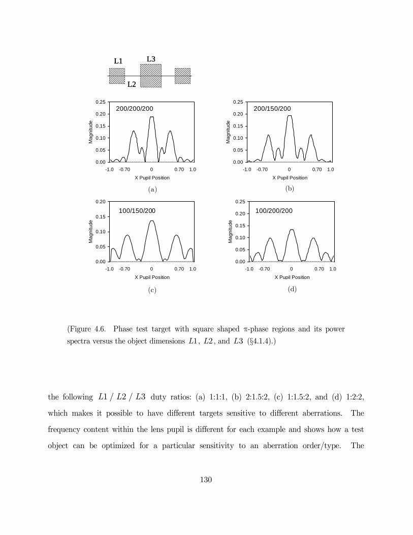
130
(Figure 4.6. Phase test target with square shaped p-phase regions and its power
spectra versus the object dimensions , , and (§4.1.4).)
the following 1 / 2 / 3L L L duty ratios: (a) 1:1:1, (b) 2:1.5:2, (c) 1:1.5:2, and (d) 1:2:2,
which makes it possible to have different targets sensitive to different aberrations. The
frequency content within the lens pupil is different for each example and shows how a test
object can be optimized for a particular sensitivity to an aberration order/type. The
1L 2L 3L
0.00
0.05
0.10
0.15
0.20
0.25
X Pupil Position
Mag
nitu
de
-1.0 -0.70 0 0.70 1.0
0.00
0.05
0.10
0.15
0.20
0.25
X Pupil Position
Mag
nitu
de
-1.0 -0.70 0 0.70 1.0
0.00
0.05
0.10
0.15
0.20
0.25
X Pupil Position
Mag
nitu
de
-1.0 -0.70 0 0.70 1.0
0.00
0.05
0.10
0.15
0.20
0.25
X Pupil Position
Mag
nitu
de
-1.0 -0.70 0 0.70 1.0
0.00
0.05
0.10
0.15
0.20
X Pupil Position
Mag
nitu
de
-1.0 -0.70 0 0.70 1.0
0.00
0.05
0.10
0.15
0.20
X Pupil Position
Mag
nitu
de
-1.0 -0.70 0 0.70 1.0
0.00
0.05
0.10
0.15
0.20
0.25
X Pupil Position
Mag
nitu
de
-1.0 -0.70 0 0.70 1.0
0.00
0.05
0.10
0.15
0.20
0.25
X Pupil Position
Mag
nitu
de
-1.0 -0.70 0 0.70 1.0
L1
L2
L3L1
L2
L3
200/200/200 200/150/200
100/150/200 100/200/200
(b)(a)
(d)(c)

131
diffraction energy distribution of Figure 4.6(c), for example, is most sensitive to third order
(or primary) aberrations.
Since aberrations are unique in ways they influence specific portions of a lens pupil, designing
an aberration test target so that it will sample a lens pupil in the most effective way is
possible. The objective is to determine the optimum combination of features that fully
samples a pupil. The test target can be designed so that it is most sensitive to particular
aberration types and order.
Several factors are considered in designing the optimal target design such that a target image
yields a high level of correlation with as many aberrations as possible. Ideally, the method
must work with a target that has both a high sensitivity to aberrations and a low cross-
correlation between different fit parameters. The method does not impose a restriction on
the target choice, so long as the pupil is adequately sampled. Target sensitivities can be
determined with print tests or by simulation. A print test example is shown in Figure 5.8.
A combination of imaging test structures with a linear model makes it possible to obtain a
theoretical function (sensitivity) of shape parameter to aberration. The theoretical
sensitivity is calculated using the PROLITH program (KLA-Tencor, 2007), a commercial
software package for optical lithography simulation. In order to increase the sensitivity of
detection method to higher order aberrations, flexibility is needed to selectively change the
targets used.
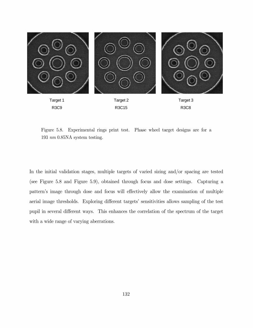
Fig
193
In the in
(see Figu
pattern’s
aerial im
pupil in
with a w
Target 1
R3C9
gure 5.8. E
3 nm 0.85NA
nitial valida
ure 5.8 and
s image thro
mage thresho
several diffe
wide range of
Experimental
A system test
ation stages,
d Figure 5.9
ough dose
olds. Explor
erent ways.
f varying ab
Ta
R3
rings print
ting.
, multiple t
9), obtained
and focus w
ring differen
This enha
berrations.
132
arget 2
3C15
t test. Pha
targets of va
d through f
will effective
nt targets’ s
ances the co
ase wheel ta
aried sizing
focus and d
ely allow th
sensitivities
orrelation of
Target
R3C8
arget designs
g and/or sp
dose settings
he examina
allows sam
f the spectru
t 3
8
s are for a
acing are te
s. Capturi
ation of mul
mpling of the
um of the ta
ested
ing a
ltiple
e test
arget
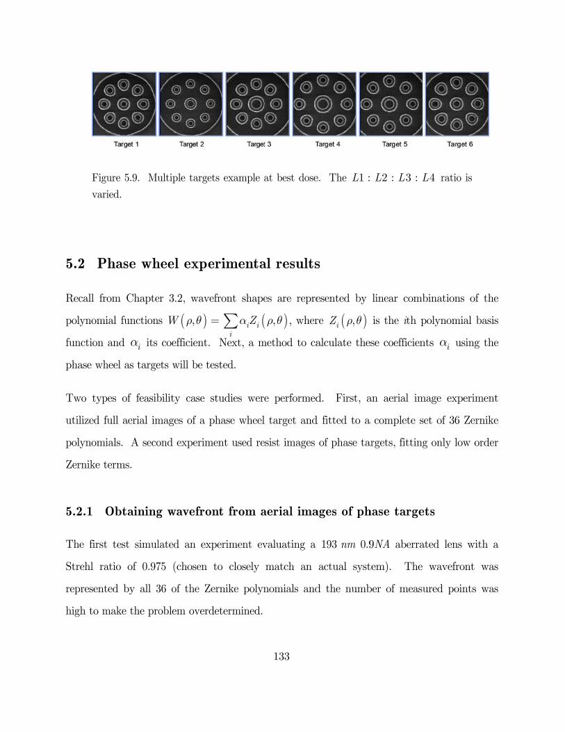
Fig
var
5.2 P
Recall fr
polynom
function
phase wh
Two typ
utilized f
polynom
Zernike t
5.2.1 O
The first
Strehl ra
represent
high to m
gure 5.9. Mu
ried.
Phase wh
rom Chapte
ial function
and ia its
heel as targe
pes of feasib
full aerial im
ials. A seco
terms.
Obtaining
t test simul
atio of 0.97
ted by all 3
make the pro
ultiple targe
heel expe
er 3.2, wave
s ( ),W r q =
coefficient.
ets will be te
bility case s
mages of a p
ond experim
g wavefro
lated an exp
75 (chosen
36 of the Ze
oblem overd
ets example a
erimenta
efront shape
(i ii
Za= å Next, a m
ested.
studies wer
phase wheel
ment used re
nt from a
periment ev
to closely
ernike polyn
determined.
133
at best dose
al results
es are repre
( ),r q , wher
method to ca
e performed
l target and
esist images
aerial ima
valuating a
match an
nomials and
e. The 1 :L
s
esented by
re ( ),iZ r q
alculate the
d. First, a
d fitted to a
of phase ta
ages of ph
193 nm 0.9
actual syst
d the numb
2 : 3 :L L L
linear comb
is the ith p
ese coefficien
an aerial im
a complete s
argets, fitting
hase targe
9NA aberra
tem). The
ber of measu
4L ratio is
binations of
polynomial
nts ia using
mage experim
set of 36 Zer
g only low o
ets
ated lens wi
wavefront
ured points
f the
basis
g the
ment
rnike
order
ith a
was
s was
134
The input to the model was a 2D aerial image intensity degraded by a known amount of
aberration. Simulated aerial images were taken from a single target, with single illumination
condition (s=0.3) and at three planes of focus.
As shown in Figure 5.10, one input image is the in-focus image while the remainders are at
0.15 microns to either side of the best focus. To improve the stability of method, additional
image information from several image planes in the focal region was incorporated,
reminiscent of the phase diversity method by Gonsalves (1982). Defocusing perturbs an
image with an additional known phase error. The relative quadratic phase difference that
results is encoded within the each image.
The procedure involved precisely modeling the propagation of light from the mask to the
wafer using PROLITH, and subsequently comparing the simulated images of phase wheels
against the synthetic images.
As the fitting procedure was performed to determine the coefficients, the response at three
focal planes was minimized jointly. The purpose of the fit was to find the aberration
polynomial coefficients that best represent the measured image data. This example explored
two best-fit numerical solutions for 36 parameters simultaneously. A large-scale gradient-
based method was used (see Chapter 7.3). Also, a simplex search method that minimized
differences without using derivatives (while more computationally intensive) also performed
well. In this first experiment, the first 36 Zernike terms up through the 9th order, excluding
the piston term were determined. The coefficients for tilts x and y ( 2Z and 3Z ,
respectively) were kept zero.
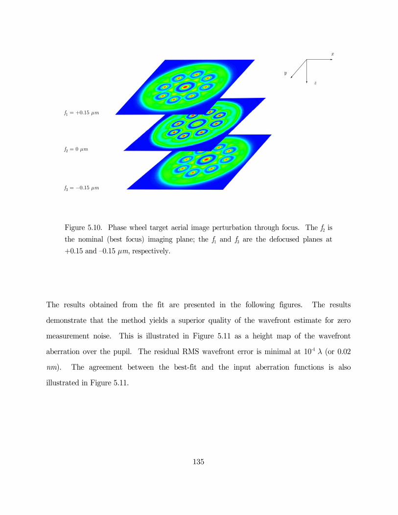
135
Figure 5.10. Phase wheel target aerial image perturbation through focus. The f2 is
the nominal (best focus) imaging plane; the f1 and f3 are the defocused planes at
+0.15 and –0.15 μm, respectively.
The results obtained from the fit are presented in the following figures. The results
demonstrate that the method yields a superior quality of the wavefront estimate for zero
measurement noise. This is illustrated in Figure 5.11 as a height map of the wavefront
aberration over the pupil. The residual RMS wavefront error is minimal at 10-4 l (or 0.02
nm). The agreement between the best-fit and the input aberration functions is also
illustrated in Figure 5.11.
y
x
z
f1 = +0.15 mm
f2 = 0 mm
f3 = -0.15 mm
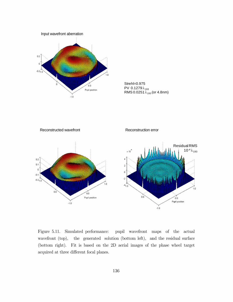
In
Re
Fig
wav
(bo
acq
nput wavefront
econstructed w
gure 5.11. S
vefront (top
ottom right)
quired at thr
t aberration
wavefront
Simulated p
), the ge
. Fit is ba
ee different f
performance:
nerated sol
ased on the
focal planes.
136
Rec
pupil w
lution (botto
2D aerial i
StrePV RMS
construction e
wavefront m
om left), an
images of th
hl=0.9750.1279 193
S 0.0251 193 (
error
maps of t
nd the resid
he phase w
R
(or 4.8nm)
the actual
dual surface
wheel target
Residual RMS10-4 193
S
3
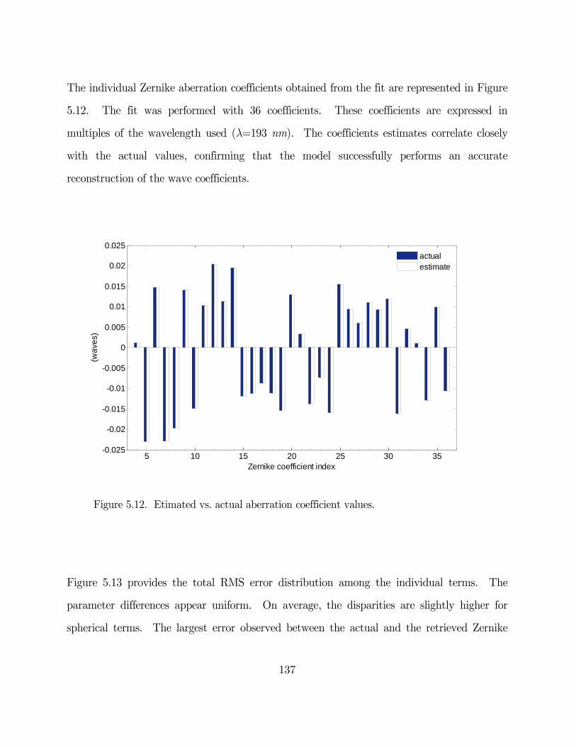
137
The individual Zernike aberration coefficients obtained from the fit are represented in Figure
5.12. The fit was performed with 36 coefficients. These coefficients are expressed in
multiples of the wavelength used (l=193 nm). The coefficients estimates correlate closely
with the actual values, confirming that the model successfully performs an accurate
reconstruction of the wave coefficients.
Figure 5.12. Etimated vs. actual aberration coefficient values.
Figure 5.13 provides the total RMS error distribution among the individual terms. The
parameter differences appear uniform. On average, the disparities are slightly higher for
spherical terms. The largest error observed between the actual and the retrieved Zernike
5 10 15 20 25 30 35-0.025
-0.02
-0.015
-0.01
-0.005
0
0.005
0.01
0.015
0.02
0.025
Zernike coefficient index
(wa
ves)
actualestimate
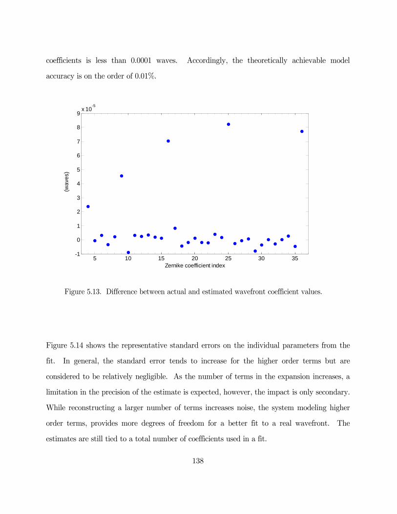
138
coefficients is less than 0.0001 waves. Accordingly, the theoretically achievable model
accuracy is on the order of 0.01%.
Figure 5.13. Difference between actual and estimated wavefront coefficient values.
Figure 5.14 shows the representative standard errors on the individual parameters from the
fit. In general, the standard error tends to increase for the higher order terms but are
considered to be relatively negligible. As the number of terms in the expansion increases, a
limitation in the precision of the estimate is expected, however, the impact is only secondary.
While reconstructing a larger number of terms increases noise, the system modeling higher
order terms, provides more degrees of freedom for a better fit to a real wavefront. The
estimates are still tied to a total number of coefficients used in a fit.
5 10 15 20 25 30 35-1
0
1
2
3
4
5
6
7
8
9x 10
-5
Zernike coefficient index
(wa
ves)
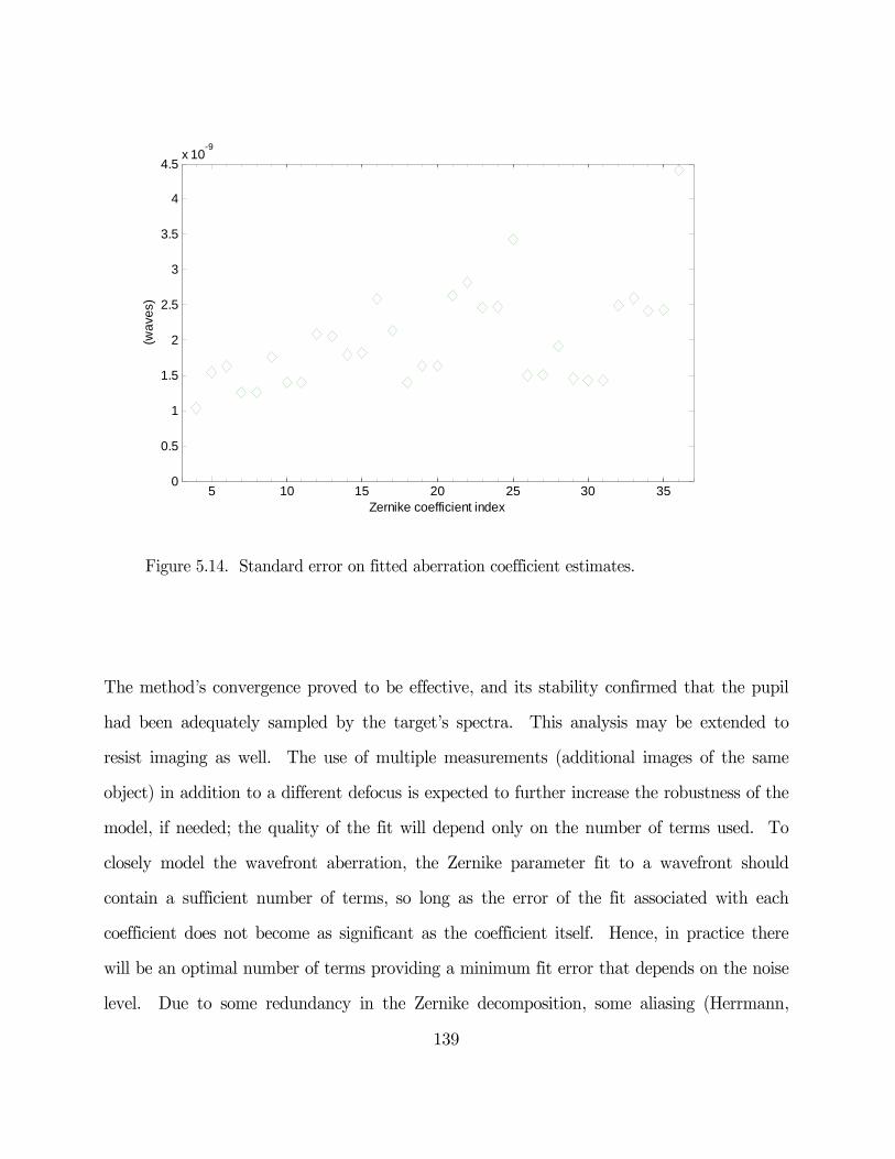
139
Figure 5.14. Standard error on fitted aberration coefficient estimates.
The method’s convergence proved to be effective, and its stability confirmed that the pupil
had been adequately sampled by the target’s spectra. This analysis may be extended to
resist imaging as well. The use of multiple measurements (additional images of the same
object) in addition to a different defocus is expected to further increase the robustness of the
model, if needed; the quality of the fit will depend only on the number of terms used. To
closely model the wavefront aberration, the Zernike parameter fit to a wavefront should
contain a sufficient number of terms, so long as the error of the fit associated with each
coefficient does not become as significant as the coefficient itself. Hence, in practice there
will be an optimal number of terms providing a minimum fit error that depends on the noise
level. Due to some redundancy in the Zernike decomposition, some aliasing (Herrmann,
5 10 15 20 25 30 350
0.5
1
1.5
2
2.5
3
3.5
4
4.5x 10
-9
Zernike coefficient index
(wa
ves)
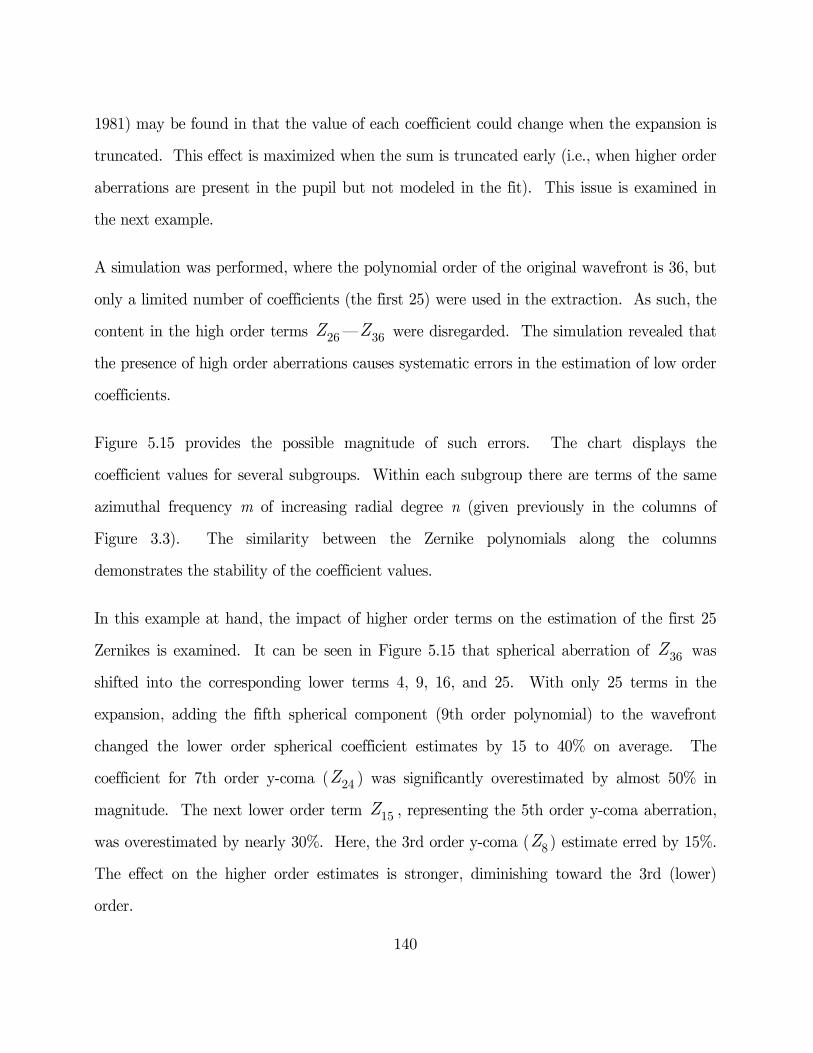
140
1981) may be found in that the value of each coefficient could change when the expansion is
truncated. This effect is maximized when the sum is truncated early (i.e., when higher order
aberrations are present in the pupil but not modeled in the fit). This issue is examined in
the next example.
A simulation was performed, where the polynomial order of the original wavefront is 36, but
only a limited number of coefficients (the first 25) were used in the extraction. As such, the
content in the high order terms 26Z — 36Z were disregarded. The simulation revealed that
the presence of high order aberrations causes systematic errors in the estimation of low order
coefficients.
Figure 5.15 provides the possible magnitude of such errors. The chart displays the
coefficient values for several subgroups. Within each subgroup there are terms of the same
azimuthal frequency m of increasing radial degree n (given previously in the columns of
Figure 3.3). The similarity between the Zernike polynomials along the columns
demonstrates the stability of the coefficient values.
In this example at hand, the impact of higher order terms on the estimation of the first 25
Zernikes is examined. It can be seen in Figure 5.15 that spherical aberration of 36Z was
shifted into the corresponding lower terms 4, 9, 16, and 25. With only 25 terms in the
expansion, adding the fifth spherical component (9th order polynomial) to the wavefront
changed the lower order spherical coefficient estimates by 15 to 40% on average. The
coefficient for 7th order y-coma ( 24Z ) was significantly overestimated by almost 50% in
magnitude. The next lower order term 15Z , representing the 5th order y-coma aberration,
was overestimated by nearly 30%. Here, the 3rd order y-coma ( 8Z ) estimate erred by 15%.
The effect on the higher order estimates is stronger, diminishing toward the 3rd (lower)
order.
141
This phenomenon affects each Zernike group more or less equally and increases the total
RMS wavefront error by 1.6 nm as well. Depending on the amount of high order aberration
present, the error in extracted coefficients is expected to rise to 100% (as in the m = 3
subgroup). This behavior results in the form of aliasing, which in this context is a low order
aberration estimated in the presence of higher order errors occurring with the truncated fits.
But, as confirmed by the first experimental study, this error can be corrected by extracting a
complete set of 36 Zernike coefficients. Consequently, because high order aberrations are
always present, calculations of both low and high order Zernike terms are necessary for
accurate fit.
Selecting an appropriate number of fit parameters is critical to final accuracy. The accuracy
of the model will depend on the number of coefficients in the fit and may include a loss-
benefit between validity and noise. A large enough number of Zernike coefficients in the
modeled wavefront is essential to distinguish the magnitude of aberration terms in lenses
with significant amounts of higher order aberrations (see example supplied in §6.5.1).
142
Figure 5.15. In this example, we check the validity of truncating the fit, which could
lead to interaction between orders. The wavefront solution is given when expansion
is truncated at index i=25. Higher order coefficients ( 26a — 36a ) while present were
excluded from the fit. Charted by subgroup (about the individual columns in
Fig. 3.3), m=0 represents spherical aberration terms (4, 9, 16, and 25), m=1 comatic
x terms (7, 14, 23, and 34), m=2 astigmatic, and so on. The effect of high orders
aberration is noticeable at low orders. The solution is generally unsatisfactory and
higher order coefficients must be included in the fit.
4 9 16 25 36-0.02
0
0.02
m=
0
7 14 23 34
-0.02
0
0.02
m=
1
8 15 24 35
-0.02
0
0.02
m=
1
5 12 21 32
-0.02
0
0.02
m=
2
6 13 22 33-0.02
0
0.02
m=
2
10 19 30
-0.02
0
0.02
m=
3
11 20 25 31-0.02
0
0.02
Zernike coefficient index
m=
3
actual
truncated fit
143
5.2.2 Obtaining wavefront from resist images of phase targets
In the second feasibility case study, the method was tested in a projection exposure tool
using image measurements in resist. A high numerical aperture, small-field 157 nm
lithography lens was evaluated. The information about lens errors was extracted from
multiple SEM images of the phase wheel object taken at the ~0.3l defocus step (phase
difference). The wavefront decomposition was performed on a restricted wavefront (primary
spherical, astigmatism, coma, and trefoil only) on a circular aperture using PROLITH
v.9.3.2.2 full vector simulation. A simple photoresist development model was used, known as
the threshold model, to relate the image intensity distribution to the printed photoresist
dimension. This model is valid in the limit of very thin and very high contrast photoresist.
The evaluation involved experiments with different relative target dimensions. The 1:1.5:2,
2:2.5:2, 1.5:2.5:2 and 1:1:1.5 target sensitivities were explored. In general, smaller target sizes
tend to create increased sensitivity to both projection lens aberration and illumination errors.
Figure 5.16 shows a subset of printed resist patterns and corresponding fit contours in the
focal plane as well as out-of-focus planes. Seven SEM images, covering a range of defocus
from –0.15 to +0.15 μm, are shown. The data was used to analyze the low order aberrations
only.
The fitted wavefront estimated by low order Zernike polynomials is shown in Figure 5.17.
Figure 5.17a is a plot of the resulting aberration phase map with piston, tilts, and defocus
removed. It was established that the lens wavefront dominant aberrations were astigmatism
5Z and 6Z , followed at a much lower level by spherical ( 9Z ) and trefoil y ( 11Z ). For this
0.90NA lens, the Strehl ratio is 0.927, demonstrating the ability to characterize diffraction-
limited optics using the phase wheel test. The total wavefront aberration in this example is
0.04wave RMS OPD. The phase wheel target was capable of detecting a variety of
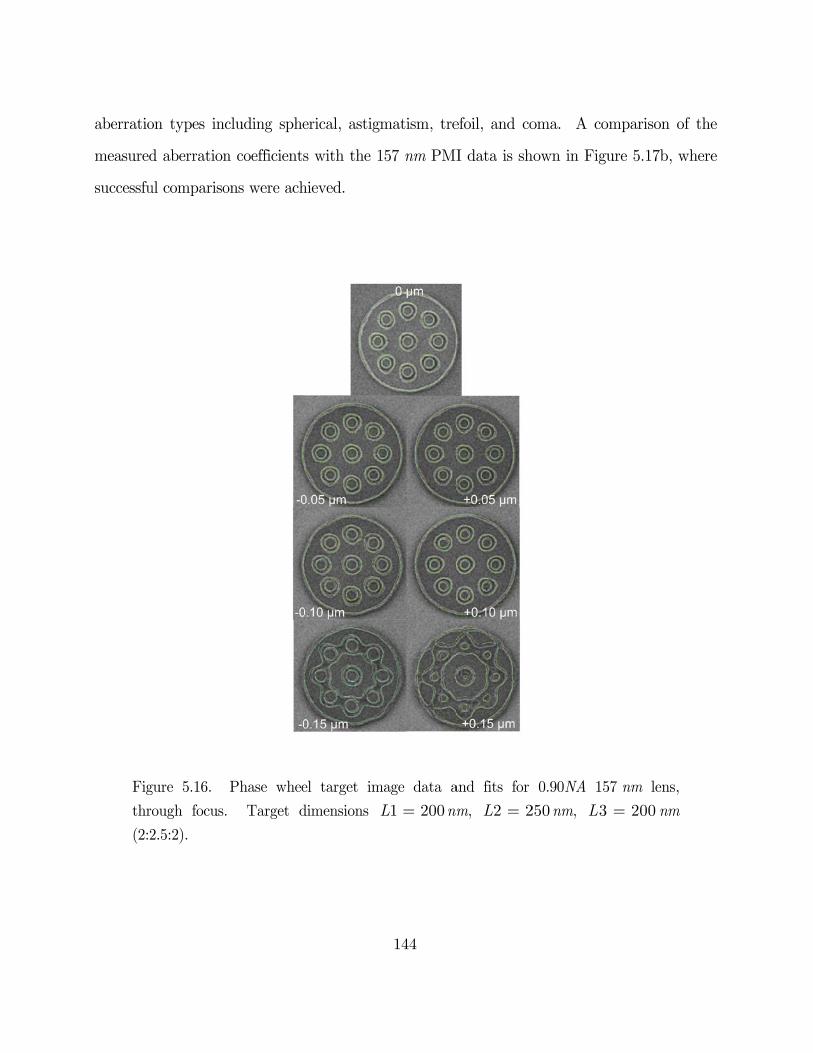
aberratio
measured
successfu
Fig
thro
(2:2
on types inc
d aberration
ul compariso
gure 5.16.
ough focus.
2.5:2).
cluding sphe
n coefficients
ons were ach
Phase whee
Target d
erical, astigm
s with the 1
hieved.
el target im
dimensions
144
matism, tre
157 nm PMI
mage data a
1 200L = n
efoil, and co
I data is sh
and fits for
m, 2 2L =
oma. A co
hown in Figu
0.90NA 15
250nm, 3L
mparison o
ure 5.17b, w
57 nm lens,
200= nm
f the
where
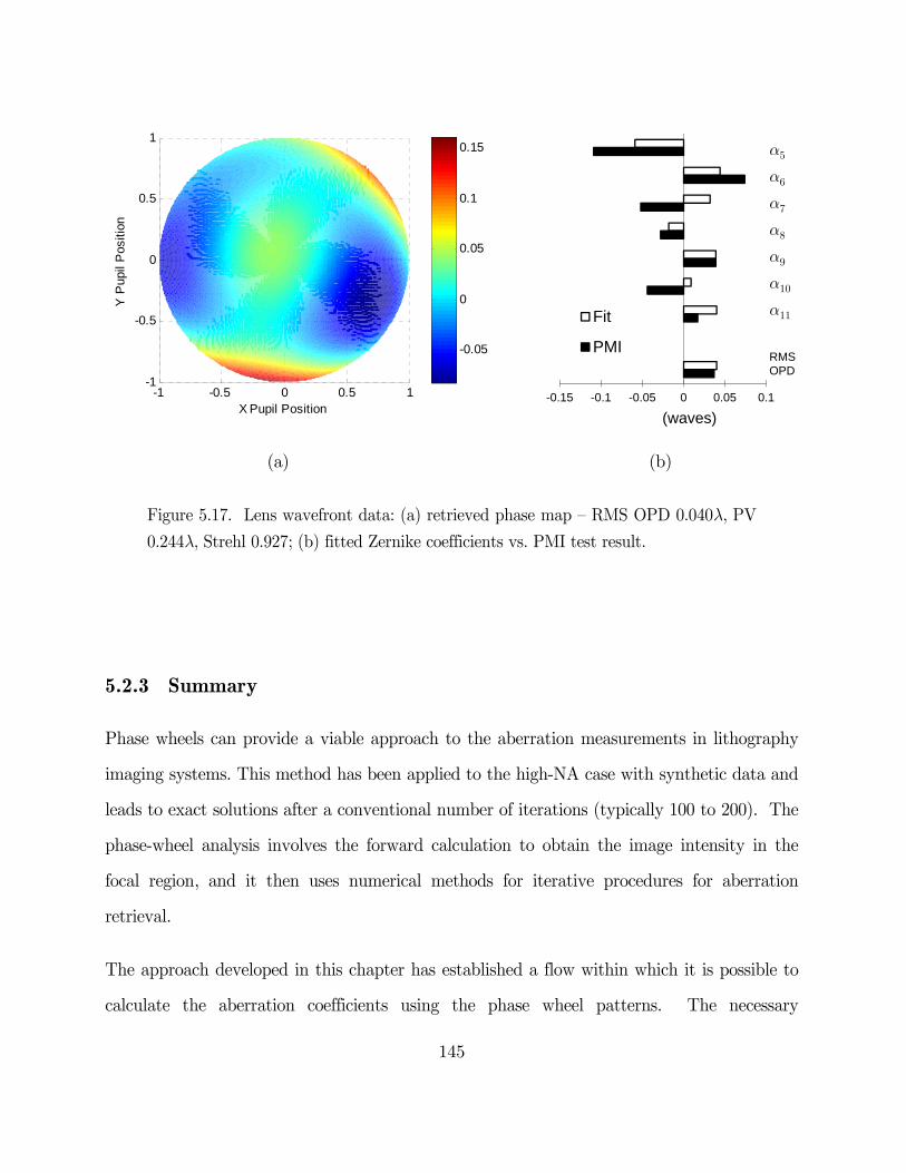
145
(a) (b)
Figure 5.17. Lens wavefront data: (a) retrieved phase map – RMS OPD 0.040l, PV
0.244l, Strehl 0.927; (b) fitted Zernike coefficients vs. PMI test result.
5.2.3 Summary
Phase wheels can provide a viable approach to the aberration measurements in lithography
imaging systems. This method has been applied to the high-NA case with synthetic data and
leads to exact solutions after a conventional number of iterations (typically 100 to 200). The
phase-wheel analysis involves the forward calculation to obtain the image intensity in the
focal region, and it then uses numerical methods for iterative procedures for aberration
retrieval.
The approach developed in this chapter has established a flow within which it is possible to
calculate the aberration coefficients using the phase wheel patterns. The necessary
-1 -0.5 0 0.5 1-1
-0.5
0
0.5
1
X Pupil Position
Y P
upil
Pos
ition
-0.05
0
0.05
0.1
0.15
-0.15 -0.1 -0.05 0 0.05 0.1
(waves)
Fit
PMI
a5
a6
a7
a8
a9
a10
a11
RMSOPD

146
benchmark was to ensure that masks designs could be fabricated and tested effectively in
resist. The experimental data and analysis described in this chapter confirmed the viability
for proceeding to full scale implementation and model formulation based on statistical
modeling.
147
6. Models and experimental
implementation
6.1 Comparison of parametric and physical models
In order to solve for unknown aberration coefficients encoded in a formed image of phase
wheels target, accurate and parsimonious models needed to be created that correlate phase
wheel image structure to aberration function. While a direct physical simulation (using
PROLITH lithography software) has been tested and rigorously describes the behavior of a
lithography imaging system, the method is not computationally efficient for use with
numerical optimization methods when solving for multiple unknowns. The lithography
process description is typically very complex requiring the comprehensive description of
physical, optical, and photochemical processes that obey Maxwell’s theory of radiative
transfer (EM equations), boundary conditions, kinetics laws of photoresist exposure reaction
and thermal reaction diffusion laws, kinetic development theory, etc. (Suzuki & Smith,
2007). Lithography simulation packages include all such mechanisms into algorithms based
on constructing equivalent mathematical models, and model parsimony is not a requirement.
A physics-based treatment is computationally intensive however, and renders its use for
148
optimization over broad multidimensional sample space impractical. Our strategy was to
build a compact approximation model that is practical for fast calculations of image
characteristics. This required the use of more simple models that are higher level
abstractions of physical models.
This chapter concerns meta-modeling (the concept of models of models) that spans from a
complex physics-based model to a regression-based model, tuned appropriately to the
aberration extraction task for which it is constructed. A meta-model is a model of
approximating the implicit input/output function characterizing relationships between inputs
and outputs in much simpler terms than full physical simulations. A common meta-
modeling technique is polynomial regression.
It is possible to build such a regression model, or response surface, matching a physical
model based strictly on feasible inputs. Here, the meta-models are based on physical
simulations and statistical analysis. This study uses a large parameter model that connects
real empirical data with multiple levels of models in between. The starting point is a
PROLITH simulation (e.g., §4.2.2. and §5.2), which is later replaced by a model that is more
efficient, mathematically compact, and deterministic. The parameterized descriptions of
phase wheels is a polynomial response function of input factors such as Zernike coefficients,
focus, and dose. Model inputs are assumed to be ideal, however, system non-idealities
and/or fabrication errors may still be included.
By their nature, interpolating models are accurate within a specified design space only. In
order for a model to have minimal error in the range and sample space being investigated,
the focus, dose and Zernike parameter space are chosen such that the actual predictive
capability of the model falls within a similar range in space. Accordingly, this response
surface model may be thought of as a simplified model based on a Taylor series
149
approximation, assuming small deviation of the solution point about the zero point. While
Zernike factors need to capture a relatively small range of values, the term allowed to have
the largest (1.0 wave) deviation from zero will be the focus term; therefore, focus is expected
to be included in many terms of the model equation. The useable focus range is mapped as
±l/NA2, the exposure range is ±10% from the nominal dose, and aberration coefficients for
Zernike polynomials 4Z through 36Z are selected, each within a 50 mwave interval. When
solving for aberration coefficients, the optimization constraints will be set based on the above
value span. The range of aberrations and the values of fixed settings (target, NA, s, etc.)
determine the application. A single NA and s setting are applied.
The remainder of this Chapter shows how parametric models are constructed and used for
computation of edge-contour functions, the implication being that it is now much more
practical to solve this large-scale estimation problem as current numerical techniques allow.
6.2 Model generation
Recall that each ring in the image set is represented by 13 parameters that describe its shape
(see Equation 4.24). Each shape parameter has a specific sensitivity to various Zernike
coefficients (to be shown in §6.2.4), as a function of dose and focus. The regression analysis
must formulate how each image shape characteristic relates to different inputs.
A response surface model is a multiple polynomial model. In its general form, the nth order
parametric model equation with multiple predictors is
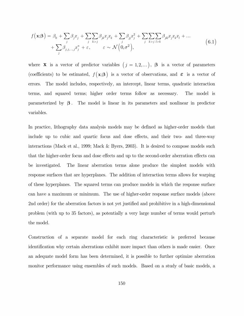
150
where x is a vector of predictor variables ( )1,2,j = , b is a vector of parameters
(coefficients) to be estimated, ( );f x b is a vector of observations, and e is a vector of
errors. The model includes, respectively, an intercept, linear terms, quadratic interaction
terms, and squared terms; higher order terms follow as necessary. The model is
parameterized by b . The model is linear in its parameters and nonlinear in predictor
variables.
In practice, lithography data analysis models may be defined as higher-order models that
include up to cubic and quartic focus and dose effects, and their two- and three-way
interactions (Mack et al., 1999; Mack & Byers, 2003). It is desired to compose models such
that the higher-order focus and dose effects and up to the second-order aberration effects can
be investigated. The linear aberration terms alone produce the simplest models with
response surfaces that are hyperplanes. The addition of interaction terms allows for warping
of these hyperplanes. The squared terms can produce models in which the response surface
can have a maximum or minimum. The use of higher-order response surface models (above
2nd order) for the aberration factors is not yet justified and prohibitive in a high-dimensional
problem (with up to 35 factors), as potentially a very large number of terms would perturb
the model.
Construction of a separate model for each ring characteristic is preferred because
identification why certain aberrations exhibit more impact than others is made easier. Once
an adequate model form has been determined, it is possible to further optimize aberration
monitor performance using ensembles of such models. Based on a study of basic models, a
( )6.1( )
( )
20
, , ,2
;
, ,0,
j j jk j k jj j jkl j k lj j k j j j k j l k
nj j j j
j
f x x x x x x x
x
b b b b b
b e e s> > >
= + + + + +
+ +
å åå å ååå
å
x
b

151
more fundamental complicated model function can be developed that is comprehensive and
mathematically more convenient. Given these considerations, a univariate multiple linear
regression model of third-order for each ring parameter as a response was chosen. The
ensembles of models for each image characteristic were then formed into one meta-model.
6.2.1 Desired regression models
Particular features of the desired model are as follows. The parameterized rings are the
response variables. The main predictor variables under study are Zernike coefficients, Zi .
(Here, the symbol Zi is used to define factor names in regression models. The symbol ia , a
notation adopted in §3.2, will continue to be used interchangeably with the Zi symbol.)
Dose, D , and defocus, F , must also be included as predictors. As indicated by the success
of the aerial-image based approach (§5.2.1), the image data must be taken through focus and
dose (i.e., taking into account the aerial image slope).
The special nature of lithography models is that focus and dose are always important, with
the need for third, sometimes fourth, order effects included in the model. Here, the model is
anticipated to be cubic in F and D terms (based on Mack (1999) lithography modeling
paper, who determined the F-D models to be 4th or 3rd order). The model is quadratic in Zi
terms.
When trying to build a simplified model, some important assumptions must also be made
about the interactions put into the model. Treating the lithographic system as a black box
implies experimentation with a model. Allowing for second and third order terms may help
resolve important interactions and improve the model. More levels of interaction are
explicitly added between dose and focus factors as well as interactions of dose/focus with all

152
aberration factors. The interactions between aberration terms are also coupled with focus
and dose to ensure occurrences of non-trivial effects were not overlooked.
The desired terms and interactions are summarized in Table 6.1.
Table 6.1. Table of desired effects and interactions.
Focus & Dose
Zernike coefficients
(i Î 4 .. 36)
1 Zi Zi2 Zi*Zj (ij)
1 X X X X
F X X X X
D X X X X
F*D X X
F2 X X
D2 X
F2*D X
D2*F X
F3 X
D3 X
As an example, to explore a 3rd order wavefront aberration (i.e., a model with ,F D , and 13
low-order Zernike coefficients ( 4Z – 16Z ) as variables), a model composed of up to 361 terms
is obtained. A custom cubic polynomial of 15 variables has 361 terms, including the desired
effects and interactions. To investigate higher order wavefront aberrations, the design

153
matrix size must be 901 for F , D , 4Z – 25Z (22 Zernike coefficients up to 7th order); and
1891 for F , D , 4Z – 36Z (33 Zernike coefficients up to 9th order).
To study this large number of effects (up to 33 Zernike factors, focus, and dose), the models
are built using an experimental design approach. The design must be adequate to
accommodate the custom cubic model with 35 main effects and 325+ higher order terms and
interactions.
6.2.2 Design generation
A response model incorporates a large number of terms and requires a design appropriate to
minimize the build cycle. To allow estimation of full third-order model for experiment
involving a large number of factors (over 30 factors), the custom cubic design provides a
reasonable response surface design option. The basic steps taken of building a custom design
are now described.
To be able to estimate the quadratic aberration effects, i.e. jjb in Equation (6.1), we need
at least three values per factor. Here we can use a Box-Behnken design (Box & Behnken,
1960), which is a common second-order design. Because we also need to consider all 3 factor
interactions, we want a custom cubic model; that is we want to construct a custom design
where we add runs to the BBD design. Other designs are perceived as too restrictive for a
very large number of factors such as we have here. The base design for Zernike coefficients,
Zi , is Box-Behnken, augmented by the addition of a full factorial in Focus and Dose F×D
for each point.
To systematically vary experimental factors, we assign each factor a discrete set of (coded)
levels. The designs are visualized in Figure 6.2.
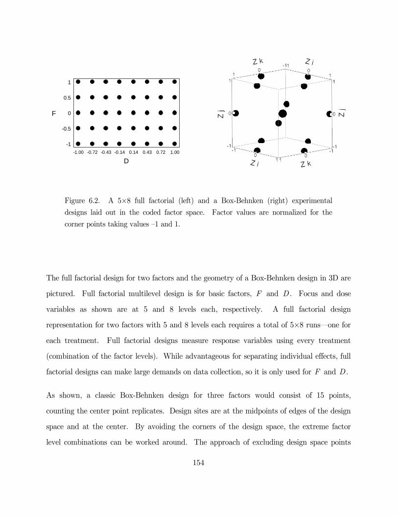
154
Figure 6.2. A 5×8 full factorial (left) and a Box-Behnken (right) experimental
designs laid out in the coded factor space. Factor values are normalized for the
corner points taking values –1 and 1.
The full factorial design for two factors and the geometry of a Box-Behnken design in 3D are
pictured. Full factorial multilevel design is for basic factors, F and D . Focus and dose
variables as shown are at 5 and 8 levels each, respectively. A full factorial design
representation for two factors with 5 and 8 levels each requires a total of 5×8 runs—one for
each treatment. Full factorial designs measure response variables using every treatment
(combination of the factor levels). While advantageous for separating individual effects, full
factorial designs can make large demands on data collection, so it is only used for F and D .
As shown, a classic Box-Behnken design for three factors would consist of 15 points,
counting the center point replicates. Design sites are at the midpoints of edges of the design
space and at the center. By avoiding the corners of the design space, the extreme factor
level combinations can be worked around. The approach of excluding design space points
-1
-0.5
0
0.5
1
F
-1.00 -0.72 -0.43 -0.14 0.14 0.43 0.72 1.00
D
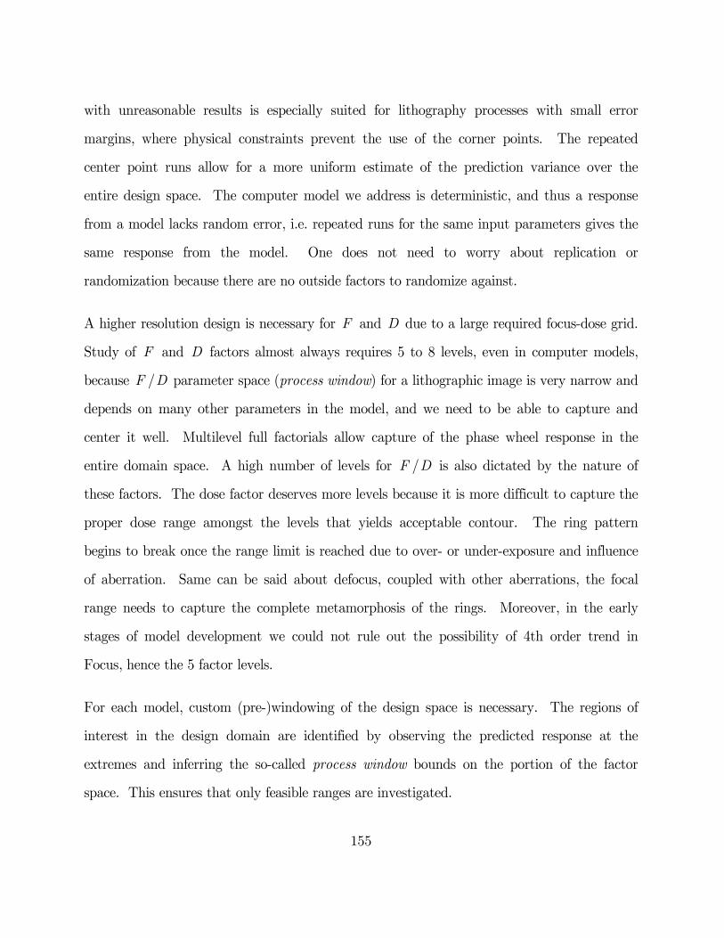
155
with unreasonable results is especially suited for lithography processes with small error
margins, where physical constraints prevent the use of the corner points. The repeated
center point runs allow for a more uniform estimate of the prediction variance over the
entire design space. The computer model we address is deterministic, and thus a response
from a model lacks random error, i.e. repeated runs for the same input parameters gives the
same response from the model. One does not need to worry about replication or
randomization because there are no outside factors to randomize against.
A higher resolution design is necessary for F and D due to a large required focus-dose grid.
Study of F and D factors almost always requires 5 to 8 levels, even in computer models,
because F /D parameter space (process window) for a lithographic image is very narrow and
depends on many other parameters in the model, and we need to be able to capture and
center it well. Multilevel full factorials allow capture of the phase wheel response in the
entire domain space. A high number of levels for F /D is also dictated by the nature of
these factors. The dose factor deserves more levels because it is more difficult to capture the
proper dose range amongst the levels that yields acceptable contour. The ring pattern
begins to break once the range limit is reached due to over- or under-exposure and influence
of aberration. Same can be said about defocus, coupled with other aberrations, the focal
range needs to capture the complete metamorphosis of the rings. Moreover, in the early
stages of model development we could not rule out the possibility of 4th order trend in
Focus, hence the 5 factor levels.
For each model, custom (pre-)windowing of the design space is necessary. The regions of
interest in the design domain are identified by observing the predicted response at the
extremes and inferring the so-called process window bounds on the portion of the factor
space. This ensures that only feasible ranges are investigated.

156
The design sizes (number of scenarios simulated) are: 324 design points for 13 Zernike terms,
936 design points for 22 Zernike terms, and 2124 for 33 Zernike terms, replicated for each
Focus/Dose level.
The 13-factor BBD design with 3 levels has 313 design points across the whole factor space.
The number of runs in the BBD design are 925 and 2113, for 22 and 33 factors, respectively.
Multiplying the number of Zernike levels by 5×8 Focus/Dose levels yields the total number
of simulation runs in the custom design: 12,520, 37,000, 84,520, for 13, 22 and 33 factors
respectively. To be able to handle such a large number (up to 1891) design points, the
design generation procedure was programmed in MATLAB (MathWorks, 2007).
Each submodel (response), once it is constructed, includes several hundred parameters to be
estimated to identify active factors in the design table.
6.2.3 Model selection
When building a regression model, we must consider model selection where it is investigated
how many parameters should be included in a model. The first step toward obtaining a
reduced-term response surface model is a systematic selection procedure. A stepwise
procedure was chosen for this task and a screening platform was scripted interfacing JMP
software (SAS, 2007) to streamline the model screening and analysis dealing with very large
datasets.
Since no direct knowledge of the actual form exists, a full model must be constructed and
evaluated. The assumed model consists of primary terms and potential terms and the goal
of stepwise regression technique is to eliminate unimportant terms from the model with little
or no effect on the error. The stepwise regression works by eliminating some portion of the
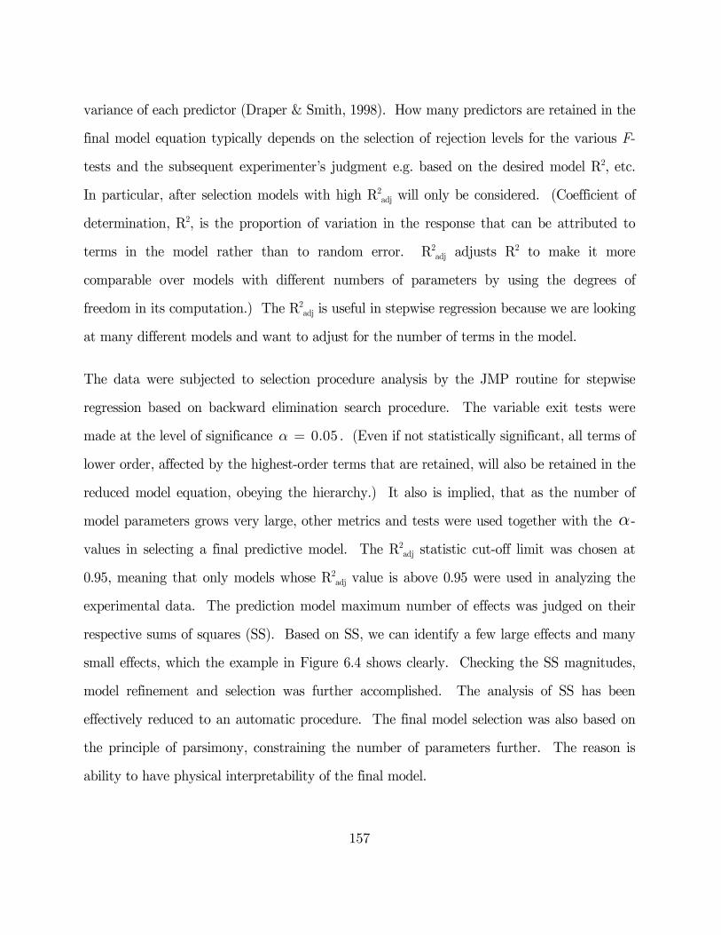
157
variance of each predictor (Draper & Smith, 1998). How many predictors are retained in the
final model equation typically depends on the selection of rejection levels for the various F-
tests and the subsequent experimenter’s judgment e.g. based on the desired model R2, etc.
In particular, after selection models with high R2adj will only be considered. (Coefficient of
determination, R2, is the proportion of variation in the response that can be attributed to
terms in the model rather than to random error. R2adj adjusts R2 to make it more
comparable over models with different numbers of parameters by using the degrees of
freedom in its computation.) The R2adj is useful in stepwise regression because we are looking
at many different models and want to adjust for the number of terms in the model.
The data were subjected to selection procedure analysis by the JMP routine for stepwise
regression based on backward elimination search procedure. The variable exit tests were
made at the level of significance 0.05a = . (Even if not statistically significant, all terms of
lower order, affected by the highest-order terms that are retained, will also be retained in the
reduced model equation, obeying the hierarchy.) It also is implied, that as the number of
model parameters grows very large, other metrics and tests were used together with the a-
values in selecting a final predictive model. The R2adj statistic cut-off limit was chosen at
0.95, meaning that only models whose R2adj value is above 0.95 were used in analyzing the
experimental data. The prediction model maximum number of effects was judged on their
respective sums of squares (SS). Based on SS, we can identify a few large effects and many
small effects, which the example in Figure 6.4 shows clearly. Checking the SS magnitudes,
model refinement and selection was further accomplished. The analysis of SS has been
effectively reduced to an automatic procedure. The final model selection was also based on
the principle of parsimony, constraining the number of parameters further. The reason is
ability to have physical interpretability of the final model.

158
The stepwise analysis has proved very effective in solving the problem of choosing a model.
From a large number of predictors, it was found effective in producing a satisfactory subset
that exhibits the strongest effects. Before model selection we started out with the full model
containing over 350 effects; after stepwise and final selection steps the reduced model had as
few as 5 terms. Response surfaces obtained after the stepwise step are shown in next
section.
6.2.4 Model analysis
Next we give several response surface model examples. The example shown in Figures 6.3
and 6.4 is the regression analysis applied to the simulated phase wheel image data,
establishing the association between ring parameter, 4s , and trefoil aberration coefficient,
11Z . A variable selection method based on stepwise (§6.2.3) was used to obtain a subset of
the predictor variables to be included in the regression model of the ring data.
When trying to determine relationships between the predictors, it is helpful to evaluate the
geometry of the response surface. Since the number of predictors makes it impossible to
visualize the entire response surface, we will use 3-, and 2-dimensional slices to obtain local
views, two factors at a time. Such low-dimensional model representation is fairly intuitive to
the lithographer accustomed to working with the Bossung plots (Bossung, 1977) and also
serves as the fit diagnostic tool.
In Figure 6.3, parameterized model is visualized in 3 dimensions. Plotted on the z-axis is 4s ,
one of several parameters (responses) used to describe the printed target. The use of a cubic
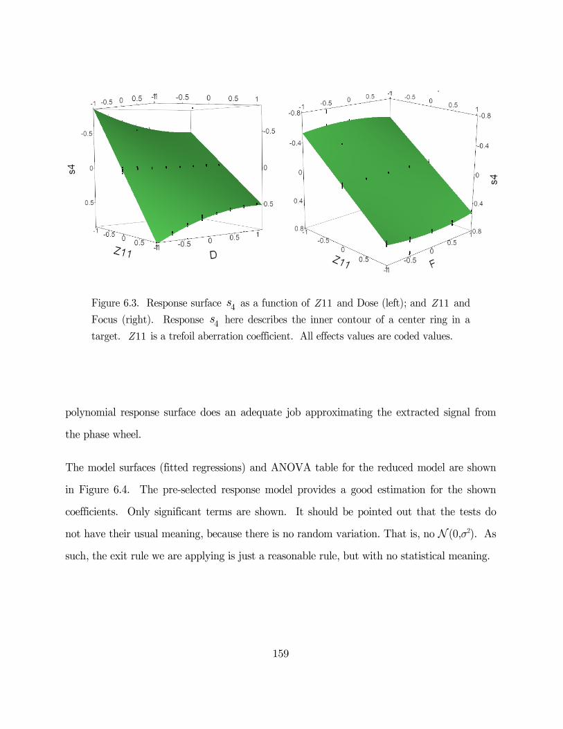
159
Figure 6.3. Response surface 4s as a function of 11Z and Dose (left); and 11Z and
Focus (right). Response 4s here describes the inner contour of a center ring in a
target. 11Z is a trefoil aberration coefficient. All effects values are coded values.
polynomial response surface does an adequate job approximating the extracted signal from
the phase wheel.
The model surfaces (fitted regressions) and ANOVA table for the reduced model are shown
in Figure 6.4. The pre-selected response model provides a good estimation for the shown
coefficients. Only significant terms are shown. It should be pointed out that the tests do
not have their usual meaning, because there is no random variation. That is, no (0,s2). As
such, the exit rule we are applying is just a reasonable rule, but with no statistical meaning.
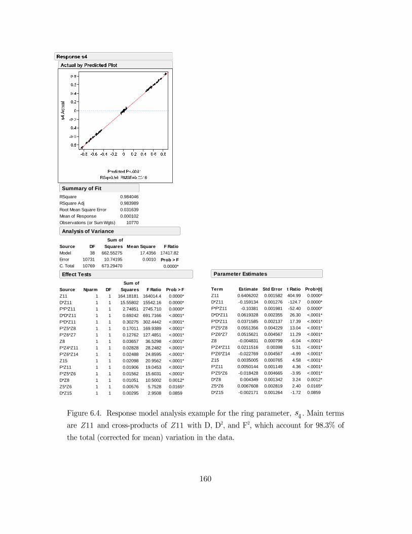
160
Figure 6.4. Response model analysis example for the ring parameter, 4s . Main terms
are 11Z and cross-products of 11Z with D, D2, and F2, which account for 98.3% of
the total (corrected for mean) variation in the data.
Z11
D*Z11
F*F*Z11
D*D*Z11
F*D*Z11
F*Z5*Z8
F*Z6*Z7
Z8
F*Z4*Z11
F*Z6*Z14
Z15
F*Z11
F*Z5*Z6
D*Z8
Z5*Z6
D*Z15
Source
1
1
1
1
1
1
1
1
1
1
1
1
1
1
1
1
Nparm
1
1
1
1
1
1
1
1
1
1
1
1
1
1
1
1
DF
164.18181
15.55802
2.74851
0.69242
0.30275
0.17011
0.12762
0.03657
0.02828
0.02488
0.02098
0.01906
0.01562
0.01051
0.00576
0.00295
Sum of
Squares
164014.4
15542.16
2745.710
691.7166
302.4442
169.9389
127.4851
36.5298
28.2482
24.8595
20.9562
19.0453
15.6031
10.5002
5.7528
2.9508
F Ratio
0.0000*
0.0000*
0.0000*
<.0001*
<.0001*
<.0001*
<.0001*
<.0001*
<.0001*
<.0001*
<.0001*
<.0001*
<.0001*
0.0012*
0.0165*
0.0859
Prob > F
Effect Tests
Z11
D*Z11
F*F*Z11
D*D*Z11
F*D*Z11
F*Z5*Z8
F*Z6*Z7
Z8
F*Z4*Z11
F*Z6*Z14
Z15
F*Z11
F*Z5*Z6
D*Z8
Z5*Z6
D*Z15
Term
0.6406202
-0.159134
-0.10381
0.0619328
0.0371585
0.0551356
0.0515621
-0.004831
0.0211516
-0.022769
0.0035005
0.0050144
-0.018428
0.004349
0.0067608
-0.002171
Estimate
0.001582
0.001276
0.001981
0.002355
0.002137
0.004229
0.004567
0.000799
0.00398
0.004567
0.000765
0.001149
0.004665
0.001342
0.002819
0.001264
Std Error
404.99
-124.7
-52.40
26.30
17.39
13.04
11.29
-6.04
5.31
-4.99
4.58
4.36
-3.95
3.24
2.40
-1.72
t Ratio
0.0000*
0.0000*
0.0000*
<.0001*
<.0001*
<.0001*
<.0001*
<.0001*
<.0001*
<.0001*
<.0001*
<.0001*
<.0001*
0.0012*
0.0165*
0.0859
Prob>|t|
Parameter Estimates
RSquare
RSquare Adj
Root Mean Square Error
Mean of Response
Observations (or Sum Wgts)
0.984046
0.983989
0.031639
0.000102
10770
Summary of Fit
Model
Error
C. Total
Source
38
10731
10769
DF
662.55275
10.74195
673.29470
Sum of
Squares
17.4356
0.0010
Mean Square
17417.82
F Ratio
0.0000*
Prob > F
Analysis of Variance
161
And so, we have described the model in a select number of terms. Interestingly, the
interactions that were found significant include those of similar aberration types, for
example, comatic terms ( 5Z , 6Z ), etc. When the model is further reduced and finalized,
special care will be taken to select among only significant effects.
Figures 6.5 and 6.6 graphically display our two other example models in three dimensions
with a surface plot, visualizing two regressors at a time. Figure 6.5 shows relationships
between 1c , F , and 5Z . Observed points (values) using 1c , F , and 5Z with the predicted
surface of fit are shown. The fit surface represents a least squares regression surface. Figure
6.6 displays a 3-dimensional surface of the 0y , 8Z , and 15Z data, at fixed values of the
other predictors.
These response surface investigations provide the initial step in a more fundamental
understanding of the system under study. Such analysis is extremely useful and enables us
to grasp the system’s behavior (via its effect on image) when many aberrations are involved.
The fact that we built a simplified model that describes a fairly complex system such as a
lithography system and solves a problem of describing arbitrary image shapes is a step
forward in our understanding how different Zernikes influence the image and is an important
learning instrument. A useful property of the regression parameters b is that they become
the so-called aberration sensitivity coefficients.
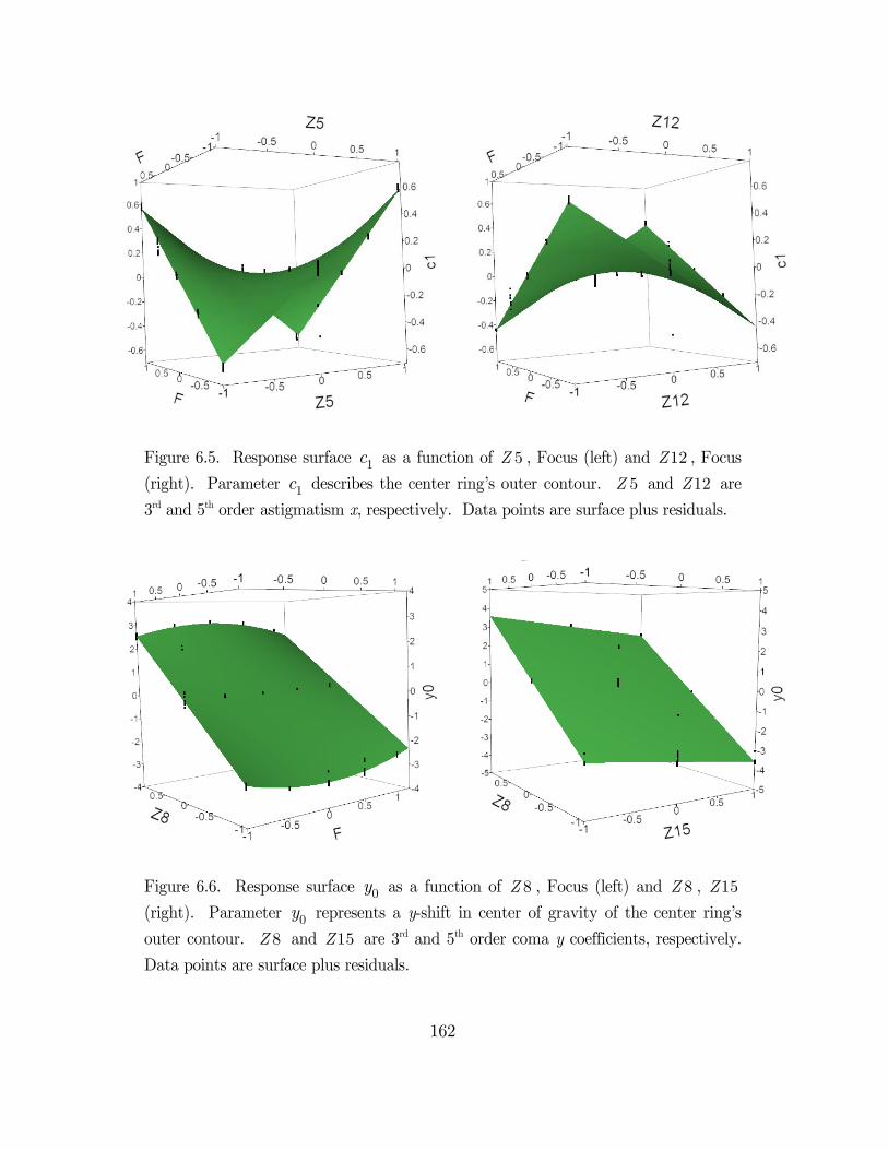
162
Figure 6.5. Response surface as a function of 5Z , Focus (left) and 12Z , Focus
(right). Parameter describes the center ring’s outer contour. 5Z and 12Z are
3rd and 5th order astigmatism x, respectively. Data points are surface plus residuals.
Figure 6.6. Response surface as a function of 8Z , Focus (left) and 8Z , 15Z
(right). Parameter represents a y-shift in center of gravity of the center ring’s
outer contour. 8Z and 15Z are 3rd and 5th order coma y coefficients, respectively.
Data points are surface plus residuals.
1c
1c
0y
0y
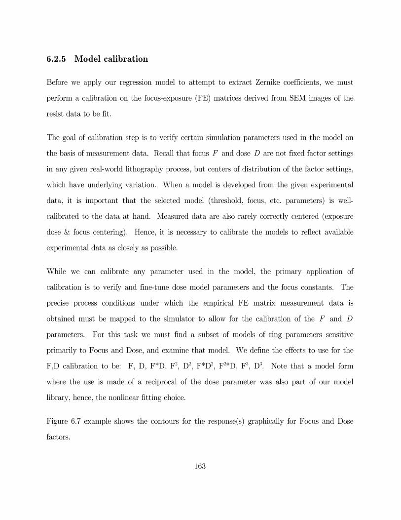
163
6.2.5 Model calibration
Before we apply our regression model to attempt to extract Zernike coefficients, we must
perform a calibration on the focus-exposure (FE) matrices derived from SEM images of the
resist data to be fit.
The goal of calibration step is to verify certain simulation parameters used in the model on
the basis of measurement data. Recall that focus F and dose D are not fixed factor settings
in any given real-world lithography process, but centers of distribution of the factor settings,
which have underlying variation. When a model is developed from the given experimental
data, it is important that the selected model (threshold, focus, etc. parameters) is well-
calibrated to the data at hand. Measured data are also rarely correctly centered (exposure
dose & focus centering). Hence, it is necessary to calibrate the models to reflect available
experimental data as closely as possible.
While we can calibrate any parameter used in the model, the primary application of
calibration is to verify and fine-tune dose model parameters and the focus constants. The
precise process conditions under which the empirical FE matrix measurement data is
obtained must be mapped to the simulator to allow for the calibration of the F and D
parameters. For this task we must find a subset of models of ring parameters sensitive
primarily to Focus and Dose, and examine that model. We define the effects to use for the
F,D calibration to be: F, D, F*D, F2, D2, F*D2, F2*D, F3, D3. Note that a model form
where the use is made of a reciprocal of the dose parameter was also part of our model
library, hence, the nonlinear fitting choice.
Figure 6.7 example shows the contours for the response(s) graphically for Focus and Dose
factors.
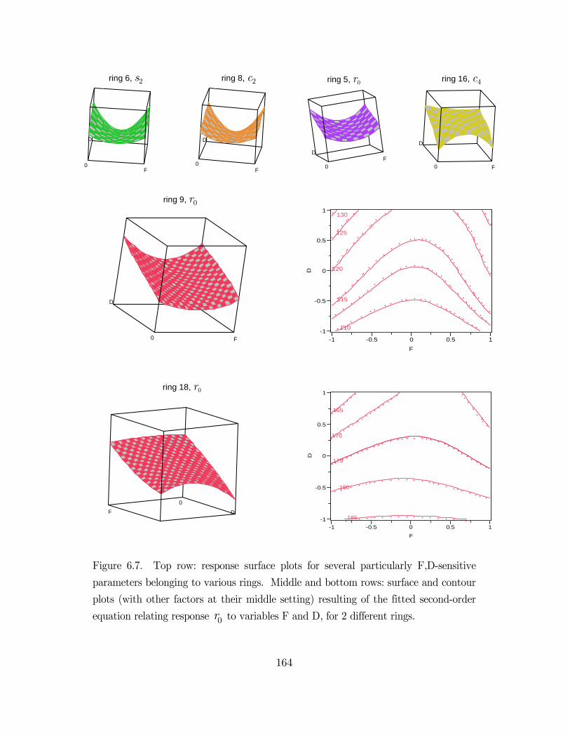
164
Figure 6.7. Top row: response surface plots for several particularly F,D-sensitive
parameters belonging to various rings. Middle and bottom rows: surface and contour
plots (with other factors at their middle setting) resulting of the fitted second-order
equation relating response 0r to variables F and D, for 2 different rings.
0F
D
R06C09
0F
D
R08C05
0F
D
R05C03
0 F
D
R16C07
0 F
D
R09C03
-1
-0.5
0
0.5
1
D
110
115
120
125
130
-1 -0.5 0 0.5 1
F
0
F D
R18C03
-1
-0.5
0
0.5
1
D
180
175
170
165
185
-1 -0.5 0 0.5 1
F
ring 6, s2 ring 8, c2 ring 16, c4ring 5, r0
ring 9, r0
ring 18, r0
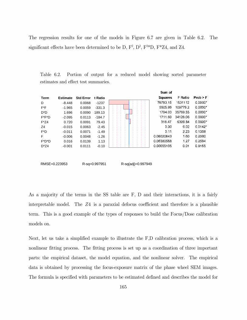
165
The regression results for one of the models in Figure 6.7 are given in Table 6.2. The
significant effects have been determined to be D, F2, D2, F2*D, F*Z4, and Z4.
Table 6.2. Portion of output for a reduced model showing sorted parameter
estimates and effect test summaries.
RMSE=0.223953 R-sq=0.997951 R-sq(adj)=0.997949
As a majority of the terms in the SS table are F, D and their interactions, it is a fairly
interpretable model. The 4Z is a paraxial defocus coefficient and therefore is a plausible
term. This is a good example of the types of responses to build the Focus/Dose calibration
models on.
Next, let us take a simplified example to illustrate the F,D calibration process, which is a
nonlinear fitting process. The fitting process is set up as a coordination of three important
parts: the empirical dataset, the model equation, and the nonlinear solver. The empirical
data is obtained by processing the focus-exposure matrix of the phase wheel SEM images.
The formula is specified with parameters to be estimated defined and describes the model for
D
F*F
D*D
F*F*D
F*Z4
Z4
F*D
F
F*D*D
D*Z4
Term
-8.448
-1.965
1.696
-2.095
0.720
-0.015
-0.011
-0.006
0.016
-0.001
Estimate
0.0068
0.0059
0.0090
0.0113
0.0091
0.0063
0.0071
0.0048
0.0139
0.0111
Std Error
-1237
-331.3
189.13
-184.7
79.43
-2.45
-1.49
-1.26
1.13
-0.10
t Ratio
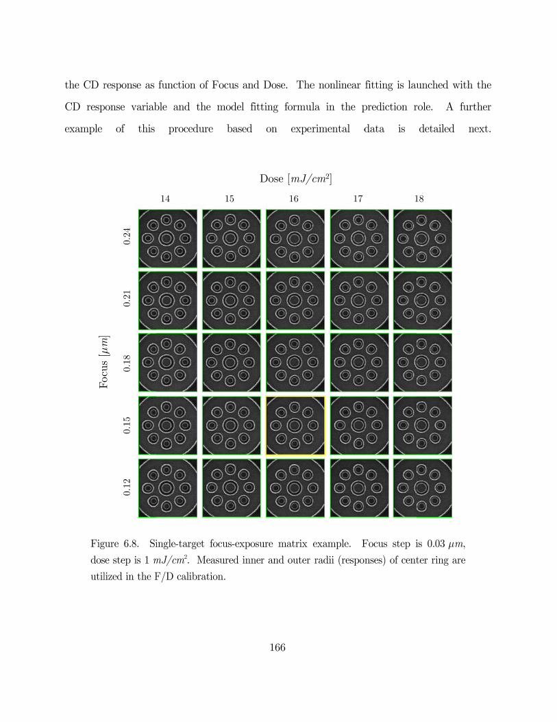
the CD r
CD resp
example
Fig
dos
util
Foc
us
[μm
]
response as
ponse variab
of this
gure 6.8. Si
se step is 1 m
lized in the F
Foc
us
[μm
]
0.12
0.15
0.
18
0
.21
0
.24
function of
ble and the
procedur
ingle-target
mJ/cm2. Me
F/D calibrat
14
f Focus and
e model fit
e based
focus-exposu
easured inne
tion.
D
15
166
Dose. The
ting formul
on exper
ure matrix
r and outer
Dose [mJ/c
16
e nonlinear
la in the p
rimental d
example. F
radii (respon
cm2]
17
fitting is lau
prediction r
data is
Focus step i
nses) of cent
1
unched with
role. A fu
detailed n
is 0.03 μm,
ter ring are
18
h the
rther
next.

167
The set of 25 images from the FEM, shown in Figure 6.8, is the empirical validation set used
on the calibration model we developed. Representative data illustrating the calibration
procedure are shown in Figure 6.9.
Suppose our response model is constructed as
The calibration model for empirical data is then
The parameter 0c is the intercept. The parameters 0f and 0d estimate the shift in nominal
focus F and dose D, respectively. The parameter 0b estimates the slope in dose
transformation. Parameter 0a should not be necessary, since it is expected to be unity. The
goal of calibration is therefore to find calibration parameters 0 0 0 0; ; ; f d b aé ùë û .
Figure 6.9 illustrates the fitting process described above. The initial values for calibration
parameters are chosen as [0, 0, 1, 1]. The nonlinear fitting process technique is very similar
to the one that will be described in §6.3 and will be omitted in this section. The final
calibration parameter estimates are 0 0 0 00.189; 36.31; 0.014; 1f d b aé ù= = = - =ë û . In
this example, the dose value of 16 mJ/cm2 corresponds to the threshold of 0.287. The plane
of best focus is found to correspond to a tool setting of 0.19 μm. The quality of the
calibration fit is excellent (R2adj is above 0.98), and thus the confidence in our image model
has been confirmed. The points on the plots in Figure 6.9 are the measured SEM image
data, and the fits are the threshold prediction by the response model. We can see that
response is reasonably close to the real values. These data suggests that the thresholded
( )6.220 1 2 1ˆ .r c f F f F d D= + * + * + * +
( )6.3( ) ( )( )
20 1 0 0 2 0 0
1 0 0
( ) ( )
( )
r c f F f a f F f a
d D d b
¢= + * - * + * - * +* - * +
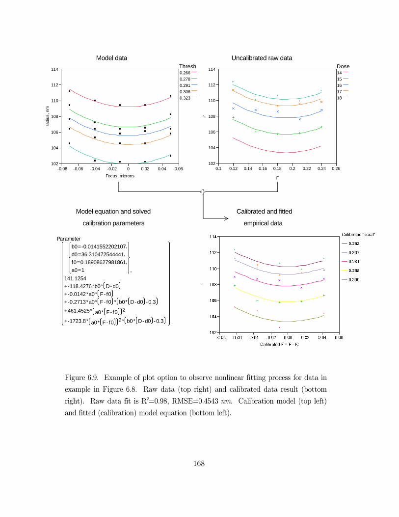
168
Model data Uncalibrated raw data
Model equation and solved Calibrated and fitted
calibration parameters empirical data
Figure 6.9. Example of plot option to observe nonlinear fitting process for data in
example in Figure 6.8. Raw data (top right) and calibrated data result (bottom
right). Raw data fit is R2=0.98, RMSE=0.4543 nm. Calibration model (top left)
and fitted (calibration) model equation (bottom left).
102
104
106
108
110
112
114
r'
0.1 0.12 0.14 0.16 0.18 0.2 0.22 0.24 0.26
F
14
15
16
17
18
Parameter
b0=-0.0141552202107,
d0=36.310472544441,
f0=0.18908627981861,
a0=1 ,
141.1254
+-118.4276*b0* D-d0
+-0.0142*a0* F- f0
+-0.2713*a0* F- f0 * b0* D-d0 -0.3
+461.4525* a0* F- f0 2
+-1723.8* a0* F- f0 2* b0* D-d0 -0.3
102
104
106
108
110
112
114
radi
us, n
m
-0.08 -0.06 -0.04 -0.02 0 0.02 0.04 0.06
Focus, microns
0.266
0.278
0.291
0.306
0.323
DoseThresh
169
aerial image model is working reasonably well and it is sufficient for building a resist model
on. This is a first in series of validation steps used to evaluate the predictive ability of this
new model.
This is an important step designed to calibrate the regression model. Recall this particular
model uses aerial image information while measured data is obtained from images measured
by SEM in photoresist. A calibration step is needed in order to correlate the aerial image
threshold from the model with dose used on the exposure tool. Similarly, the focus offset of
experimental images is calibrated based on a subset of data. The best focus aerial image is
matched with the best focus resist image.
The simple procedure developed here is very effective; Figure 6.10 illustrates the sample
calibration plots for dose and defocus with other models in Figure 6.7. (The regression
analysis for dose and focus parameters only (aberration-free case) was performed and only
rings parameters with R2adj greater than 0.95 are selected.) These are calibration plots
between the measurement point and the fit to help visualize the results of the calibration
run.
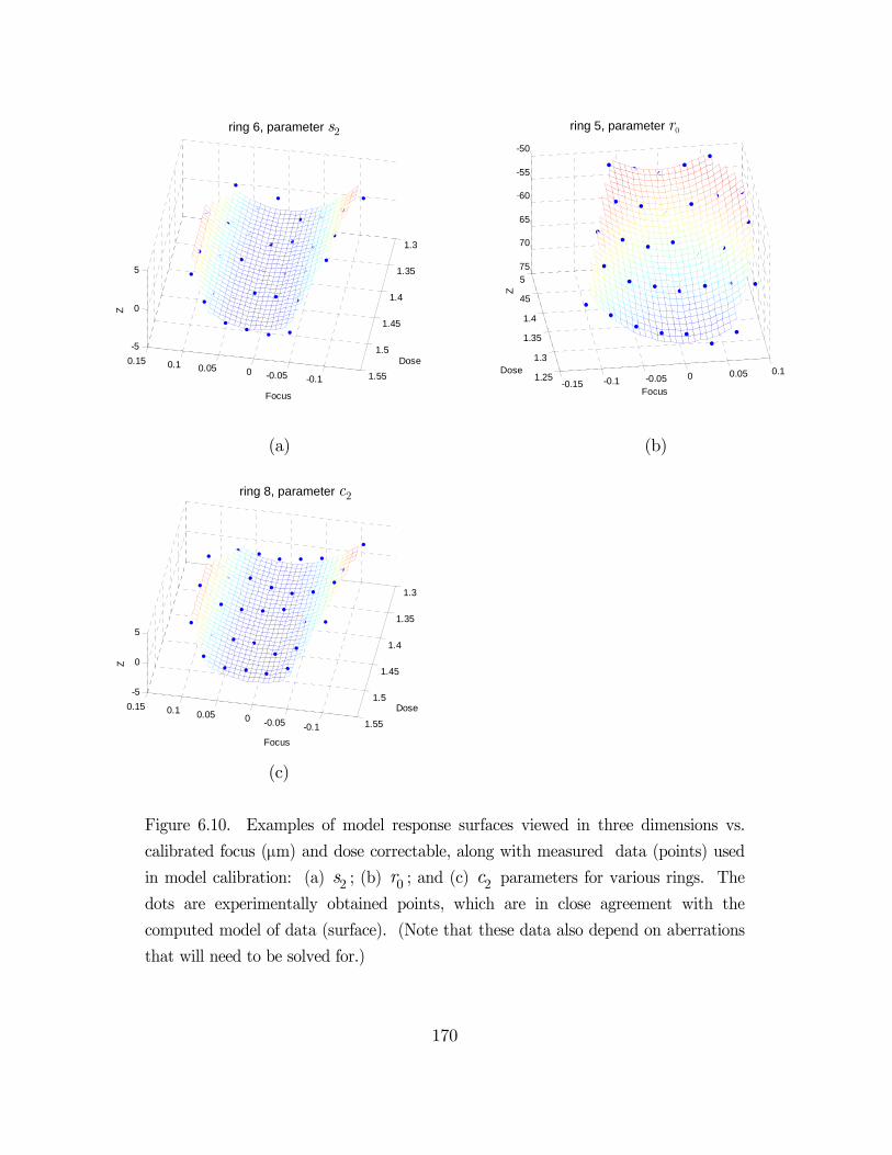
170
(a) (b)
(c)
Figure 6.10. Examples of model response surfaces viewed in three dimensions vs.
calibrated focus (μm) and dose correctable, along with measured data (points) used
in model calibration: (a) 2s ; (b) 0r ; and (c) 2c parameters for various rings. The
dots are experimentally obtained points, which are in close agreement with the
computed model of data (surface). (Note that these data also depend on aberrations
that will need to be solved for.)
-0.15 -0.1 -0.05 0 0.05 0.11.25
1.3
1.35
1.4
1.45
1.5-75
-70
-65
-60
-55
-50
Focus
Dose
Z
-0.1-0.0500.050.10.15
1.3
1.35
1.4
1.45
1.5
1.55
-5
0
5
Dose
Focus
R06C09Z
R05C03
Z
-0.1-0.0500.050.10.15
1.3
1.35
1.4
1.45
1.5
1.55
-5
0
5
Dose
Focus
R08C05
Zring 6, parameter s2
ring 8, parameter c2
ring 5, parameter r0

171
Focus and dose need to be calibrated for each photoresist process; therefore a calibration
model is built along with each aberration model. The calibration step is automatically
performed every time a dataset is analyzed. The focus-exposure lookup table created based
on this calibration fit is fed back in to the response model to tune the optimization model.
6.3 Optimization problem for aberration retrieval
Due to the way our meta-model has been constructed, Zernike parameter estimation is an n-
dimensional problem requiring a nonlinear optimization algorithm to find a numeric solution.
Since the meta-model of the optical system is not invertible, a numerical approach must be
used. Thus numerical methods are required to find a solution for estimates iteratively.
The optimization algorithm works by cancellation of errors, that is it estimates the
aberration coefficients by finding a minimum norm solution to a nonlinear least squares
problem. The evaluation metric are residuals from fit (that quantify the difference between
experimental and model-generated data), which depends on a number of iterations (function
evaluations) during the course of optimization.
The computational aspects of the optimization problem are as follows. Suppose that
( );f x a is the model. Then the nonlinear algorithm attempts to minimize the cost function
written as
where ( )o ⋅ function is squared-residuals, which is the error between the predicted value and
the actual value
( )6.4( ) ( )( )1
; ,i
N
i
L fo=
= å x aa
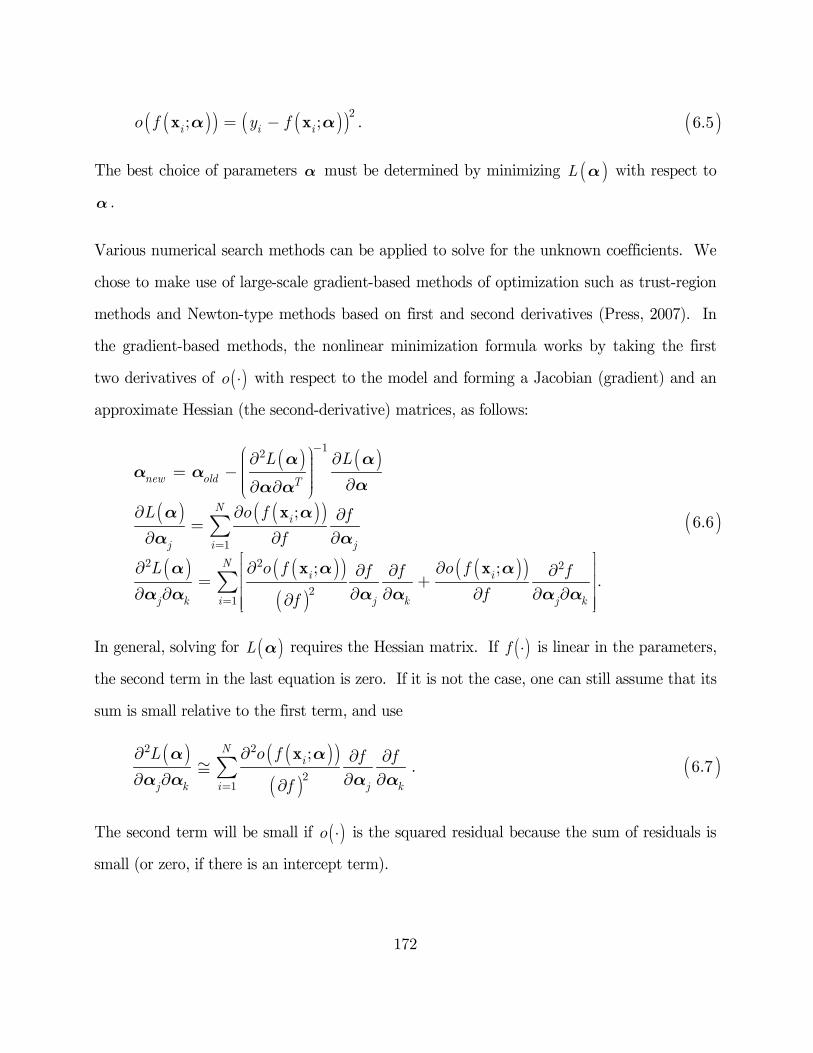
172
The best choice of parameters a must be determined by minimizing ( )L a with respect to
a .
Various numerical search methods can be applied to solve for the unknown coefficients. We
chose to make use of large-scale gradient-based methods of optimization such as trust-region
methods and Newton-type methods based on first and second derivatives (Press, 2007). In
the gradient-based methods, the nonlinear minimization formula works by taking the first
two derivatives of ( )o ⋅ with respect to the model and forming a Jacobian (gradient) and an
approximate Hessian (the second-derivative) matrices, as follows:
In general, solving for ( )L a requires the Hessian matrix. If ( )f ⋅ is linear in the parameters,
the second term in the last equation is zero. If it is not the case, one can still assume that its
sum is small relative to the first term, and use
The second term will be small if ( )o ⋅ is the squared residual because the sum of residuals is
small (or zero, if there is an intercept term).
( )6.5( )( ) ( )( )2; .;ii if y fo = -x xa a
( )6.6
( ) ( )
( ) ( )( )
( ) ( )( )( )
( )( )
12
1
2 2 2
21
;
;.
;
new old T
N
ij j
N
ij k j k
i
i i
j k
L L
L f f
f
L f ff f f
ff
o
o o
-
=
=
æ ö¶ ¶÷ç ÷ç= - ÷ç ÷ç ¶÷ç ¶ ¶è ø¶ ¶ ¶
=¶ ¶ ¶
é ù¶ ¶ ¶¶ ¶ ¶ê ú= +ê ú
¶ ¶ ¶ ¶ ¶ ¶ ¶ê ú¶ê úë û
å
å
x
x x
a aa a
aa aa
a a
a a aa a a a a a
a
( )6.7( ) ( )( )
( )
2 2
21
;.
N
ij k j k
iL f f f
f
o
=
¶ ¶ ¶ ¶@
¶ ¶ ¶ ¶¶å
xa aa a a a
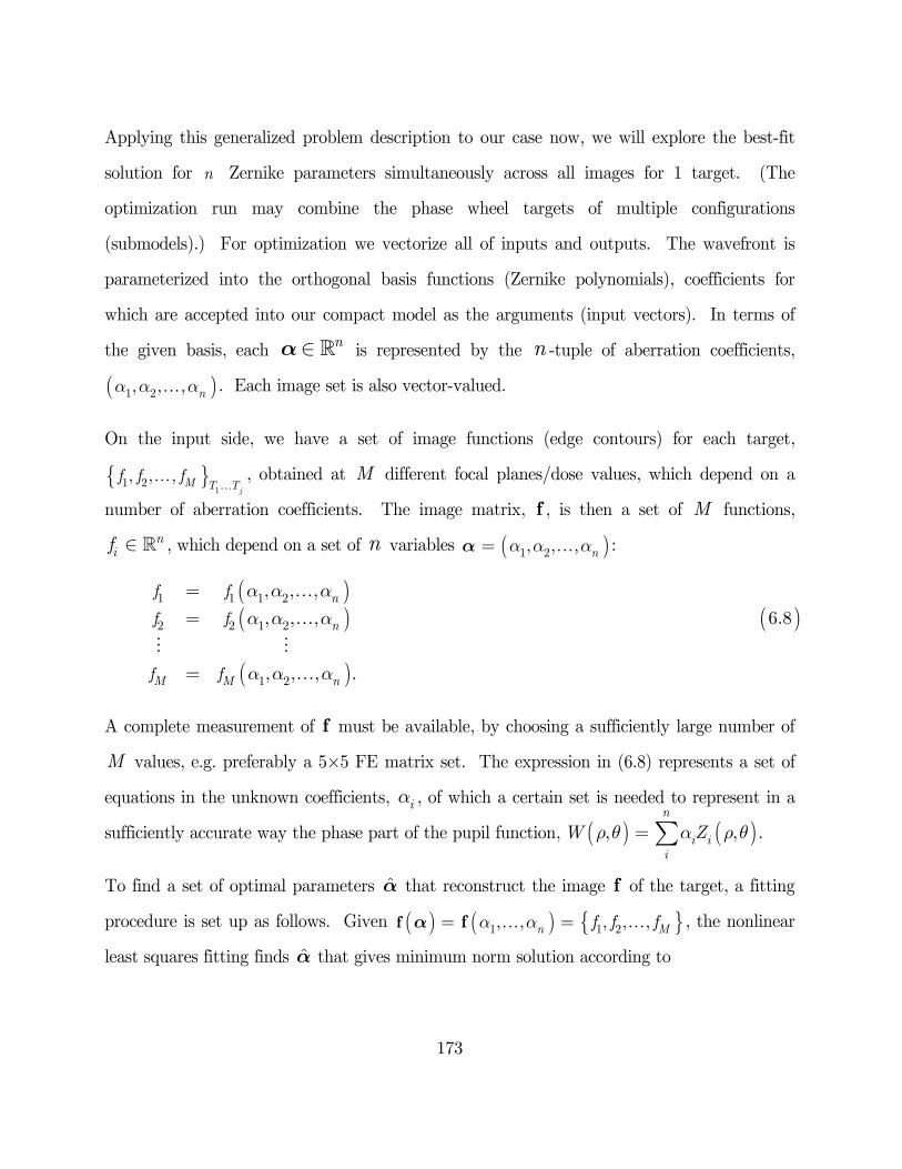
173
Applying this generalized problem description to our case now, we will explore the best-fit
solution for n Zernike parameters simultaneously across all images for 1 target. (The
optimization run may combine the phase wheel targets of multiple configurations
(submodels).) For optimization we vectorize all of inputs and outputs. The wavefront is
parameterized into the orthogonal basis functions (Zernike polynomials), coefficients for
which are accepted into our compact model as the arguments (input vectors). In terms of
the given basis, each nÎ a is represented by the n -tuple of aberration coefficients,
( )1 2, , , na a a . Each image set is also vector-valued.
On the input side, we have a set of image functions (edge contours) for each target,
{ }1
1 2, , ,j
M T Tf f f
, obtained at M different focal planes/dose values, which depend on a
number of aberration coefficients. The image matrix, f , is then a set of M functions,
nif Î , which depend on a set of n variables ( )1 2, , , na a a= a :
A complete measurement of f must be available, by choosing a sufficiently large number of
M values, e.g. preferably a 5×5 FE matrix set. The expression in (6.8) represents a set of
equations in the unknown coefficients, ia , of which a certain set is needed to represent in a
sufficiently accurate way the phase part of the pupil function, ( ) ( ), ,n
i ii
W Zr q a r q= å .
To find a set of optimal parameters a that reconstruct the image f of the target, a fitting
procedure is set up as follows. Given ( ) ( ) { }1 1 2, , , , ,n Mf f fa a= =f f a , the nonlinear
least squares fitting finds a that gives minimum norm solution according to
( )6.8
( )( )
( )
1 1 1 2
2 2 1 2
1 2
, , ,
, , ,
, , , .
n
n
M M n
f f
f f
f f
a a aa a a
a a a
==
=
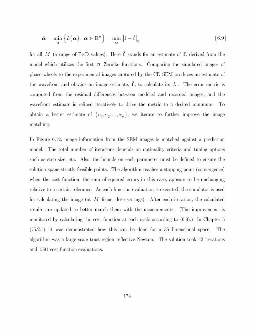
174
for all M (a range of F×D values). Here f stands for an estimate of f , derived from the
model which utilizes the first n Zernike functions. Comparing the simulated images of
phase wheels to the experimental images captured by the CD SEM produces an estimate of
the wavefront and obtains an image estimate, f , to calculate its L . The error metric is
computed from the residual differences between modeled and recorded images, and the
wavefront estimate is refined iteratively to drive the metric to a desired minimum. To
obtain a better estimate of ( )1 2, , , na a a , we iterate to further improve the image
matching.
In Figure 6.12, image information from the SEM images is matched against a prediction
model. The total number of iterations depends on optimality criteria and tuning options
such as step size, etc. Also, the bounds on each parameter must be defined to ensure the
solution spans strictly feasible points. The algorithm reaches a stopping point (convergence)
when the cost function, the sum of squared errors in this case, appears to be unchanging
relative to a certain tolerance. As each function evaluation is executed, the simulator is used
for calculating the image (at M focus, dose settings). After each iteration, the calculated
results are updated to better match them with the measurements. (The improvement is
monitored by calculating the cost function at each cycle according to (6.9).) In Chapter 5
(§5.2.1), it was demonstrated how this can be done for a 35-dimensional space. The
algorithm was a large scale trust-region reflective Newton. The solution took 42 iterations
and 1591 cost function evaluations.
( )6.9( ){ } 2ˆˆ min , minnL= Î = -f f
a aa a a
175
6.4 Solution flow overview
The full aberration extraction flow (algorithm) was exercised as outlined in Figure 6.11
below. It is subdivided into three main parts. In general, the method follows the steps of
data preparation, data analysis, modeling, and solving of an optimization problem.
The model building part of the procedure (aerial image fitting) involves precisely modeling
the propagation of light from the mask to the wafer using a lithography simulator
PROLITH, and subsequently building a meta-model.
The experimental part of the phase wheel procedure involves the generation of a focus-
exposure (FE) matrix wafer. The user performs experiment, collects the SEM data, and
feeds the images into the phase wheels software code for image processing and analysis.
The solution part requires first a F/D calibration step. In this next step, the model
calibration is based on parameters of the dataset that are independent of aberrations.
Finally, the fitting of the dataset to the supplied model is performed. The output of this is a
visualized wavefront along with the predicted Zernike coefficient. As we solve for Zernike
coefficient values, the aberration extraction is approached as an optimization problem solved
by employing numerical search methods, according to method outlined in §6.3. Using a
metamodel in multiple dimensions requires use of an optimization method to search
iteratively for the solution (fitted wavefront). The numerical fitting algorithm includes the
nonlinear optimization of the fit parameters to find the best match between model and
measured resist edges. The parameters that are known about the system a priori are used as
constraints. Once the initial (set of) images are compared, the iterative algorithm is
deployed to arrive at an estimate of Zernike aberration coefficients that give the best match
between the model and the measured image data. The error for the fit is taken as the
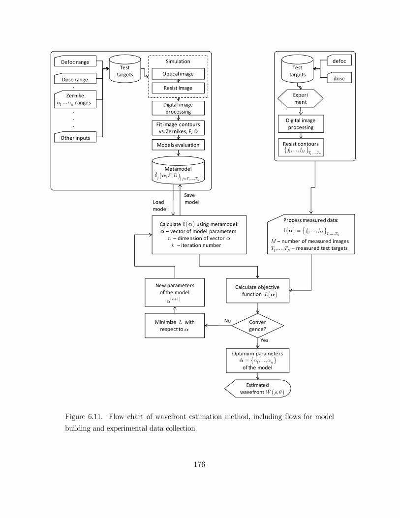
176
Figure 6.11. Flow chart of wavefront estimation method, including flows for model
building and experimental data collection.
Convergence?
Estimated wavefront W^
Process measured data:
n – number of measured imagesM – measured test targets
Calculate objective function L(a)
Minimize L( with respect to a
Optimum parameters
of the model
New parameters of the model
a^(k)
Calculate {fM} using metamodel:a – vector of model parameters
n – dimension of vector a– iteration number
Optical image
Resist image
Digital image processing
Digital image processing
Resist contours fj(F,E)
Simulation
Fit image contours vs. Zernikes, F, D
MetamodelT1…TN fj
Models evaluation
Test targets
Other inputs
ZernikeZ1… ranges
Defoc range
Dose range
SaveLoad modelmodel
Test targets
defoc
dose
.
.
.
.
Experiment
( )L a
Yes
NoL
a
( )1k +a
{ }1ˆ , , na a= a
( )ˆ ,W r q
1, , NT TM
( ) { }1
1 , ,, ,
NM T T
f f=f
aan
a( )f a
( ){ }1, ,ˆ , ,
Nj j T T
F D=
f
a
1 na a
{ }1
1 , ,, ,
NM T T
f f
k

177
difference between the experimental and reconstructed edge functions in a given dataset.
Including an initial guess for Zernike polynomial coefficients improves the fit and helps
converge faster, but is not required.
The entire fitting procedure is implemented in MATLAB as well as the rest of the code that
performs image processing and calculations and is interfaced with the lithography simulator.
MATLAB code was written to also interface JMP statistical engine (software by SAS) that
is used for model building.
The framework of computer code was developed with the goal to easily define models, gather
data, automate data processing, manage model formulations, analyze results, and perform
visualization tasks. The final program code implements the algorithms outlined in §4.2 and
§§6.1–6.3, and integrates the key steps.
The method has potential to be further refined. In addition to Zernike coefficients, the
important degrees of freedom of the imaging model include the illumination coherence factor,
numerical aperture, focus offset, target geometry, etc. All but the Zernike coefficients are
usually known for the system or, in practice, can be determined from independent
measurements. Additional flexibility can be gained in the model by including the variation
in any of these – a partial coherence, for instance. This would then take into account an
uncertainty in the partial coherence measurement.
A preliminary results assessment of fits performed using this full flow can be found in the
next section.
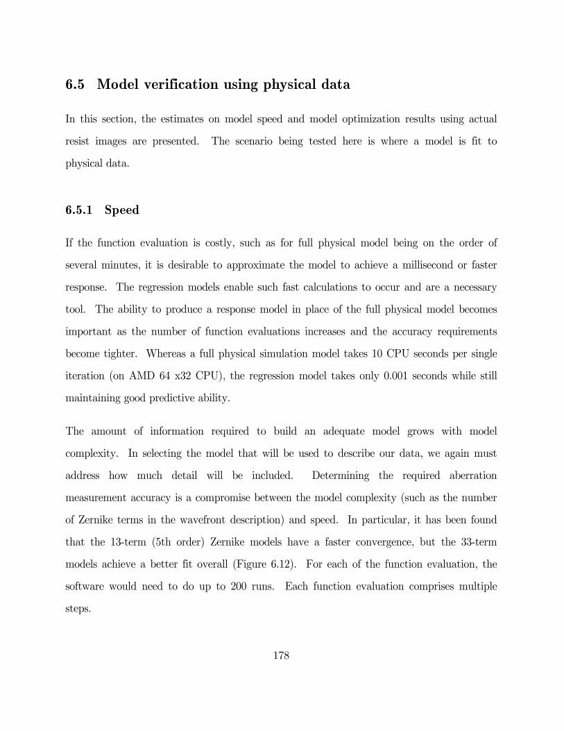
178
6.5 Model verification using physical data
In this section, the estimates on model speed and model optimization results using actual
resist images are presented. The scenario being tested here is where a model is fit to
physical data.
6.5.1 Speed
If the function evaluation is costly, such as for full physical model being on the order of
several minutes, it is desirable to approximate the model to achieve a millisecond or faster
response. The regression models enable such fast calculations to occur and are a necessary
tool. The ability to produce a response model in place of the full physical model becomes
important as the number of function evaluations increases and the accuracy requirements
become tighter. Whereas a full physical simulation model takes 10 CPU seconds per single
iteration (on AMD 64 x32 CPU), the regression model takes only 0.001 seconds while still
maintaining good predictive ability.
The amount of information required to build an adequate model grows with model
complexity. In selecting the model that will be used to describe our data, we again must
address how much detail will be included. Determining the required aberration
measurement accuracy is a compromise between the model complexity (such as the number
of Zernike terms in the wavefront description) and speed. In particular, it has been found
that the 13-term (5th order) Zernike models have a faster convergence, but the 33-term
models achieve a better fit overall (Figure 6.12). For each of the function evaluation, the
software would need to do up to 200 runs. Each function evaluation comprises multiple
steps.
179
Figure 6.12. Convergence of model solution during search iterations: 13 vs. 33 Z-
term model. The extended model is more computationally costly (to build) but
performs an order of magnitude closer reconstruction of the input function than the
short model.
6.5.2 Predictive power
To check the predictive ability of our regression model, we applied a 13-term model to the
dataset that originated in the experiment performed on a state-of-the-art step-and-scan
system. The optical system under evaluation was a l=193 nm, NA=0.85 scanner that
required astigmatism aberration characterization and correction. Most of the contribution
on image from a large third order 45 astigmatism comes as an orientation dependent best
focus position that results in the horizontal to vertical CD difference; hence, the 5Z
100
1,000
10,000
100,000
1,000,000
0 100 200 300 400 500
Number of function evaluations
33-term model
13-term modelR
MS
E f
rom
fit (
a.u.
)
180
correction was desired. Phase wheel measurements were collected before and after
astigmatism correction. The correction involved changing the position of the movable lens
elements resulting in the astigmatism term, 5Z , to be corrected by 10 mwaves – a major
adjustment. Other adjustable aberrations were unchanged.
For the case shown in Figure 6.13 we examine a set of data to which a third-order model
was fitted. The goal was to detect and quantify astigmatism that was adjusted on the tool
and compare wavefronts before and after correction. The approach was to use multiple
targets at multiple exposures through focus. Data was modeled on the 13 aberrations ( 4Z
through 16Z ) and process variables (dose and defocus).
Setting 1 represents the lens state before astigmatism 5Z correction, setting 2 is after. We
see that Zernike 5Z is the largest term for setting 1. For setting 2, the 5Z aberration has
been corrected, as also evidenced in the difference surface, which has a characteristic
astigmatism shape.
Depicted in Figure 6.13 (top left) is the wavefront before the correction. Figure 6.13 (top
right) is the fitted wavefront after the 5Z correction. For both wavefronts, the fifth order
model consisting of 13 terms ( 4Z - 16Z ) was used from three different phase wheel targets
simultaneously at a single dose through focus. Figure 6.13 bar plot (bottom right) compares
the two wavefronts term-by-term; units on the Y-axis are waves. Setting 2 aberration
magnitudes are nearly unchanged for all Zernike terms relative to setting 1, except for a 5Z
astigmatism where there is a 0.01 wave delta observed. Figure 6.13 (bottom left) displays
the amount of aberration error removed from lens by going from setting 1 to setting 2 state.
The difference between the two wavefronts highlights the astigmatism signature that has
been successfully removed upon the lens adjustment. It was independently confirmed (by
ILIAS test) that it was the astigmatism aberration 5Z , with the other Zernike variables
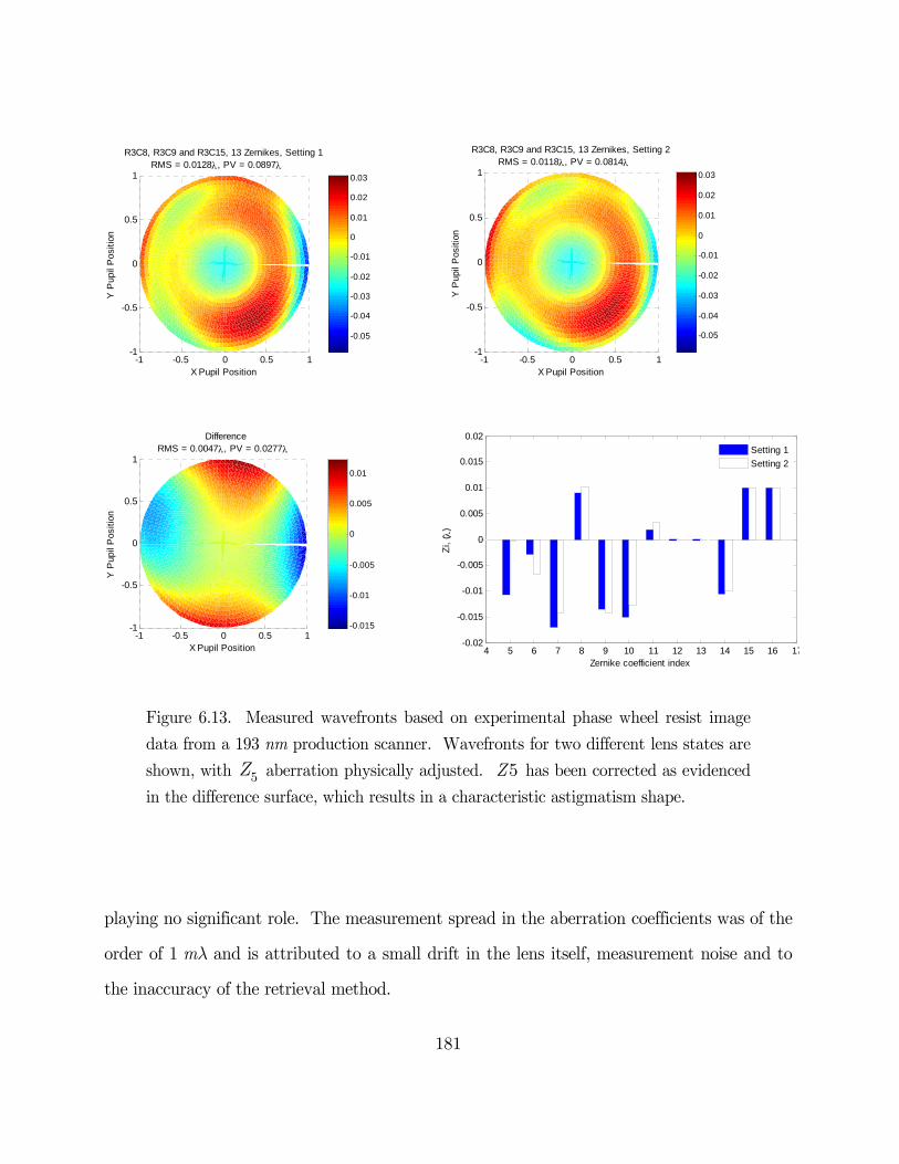
181
Figure 6.13. Measured wavefronts based on experimental phase wheel resist image
data from a 193 nm production scanner. Wavefronts for two different lens states are
shown, with 5Z aberration physically adjusted. 5Z has been corrected as evidenced
in the difference surface, which results in a characteristic astigmatism shape.
playing no significant role. The measurement spread in the aberration coefficients was of the
order of 1 ml and is attributed to a small drift in the lens itself, measurement noise and to
the inaccuracy of the retrieval method.
-1 -0.5 0 0.5 1-1
-0.5
0
0.5
1
X Pupil Position
R3C8, R3C9 and R3C15, 13 Zernikes, Setting 1RMS = 0.0128, PV = 0.0897
Y P
upil
Pos
ition
-0.05
-0.04
-0.03
-0.02
-0.01
0
0.01
0.02
0.03
-1 -0.5 0 0.5 1-1
-0.5
0
0.5
1
X Pupil Position
R3C8, R3C9 and R3C15, 13 Zernikes, Setting 2RMS = 0.0118, PV = 0.0814
Y P
upil
Pos
ition
-0.05
-0.04
-0.03
-0.02
-0.01
0
0.01
0.02
0.03
-1 -0.5 0 0.5 1-1
-0.5
0
0.5
1
Difference RMS = 0.0047, PV = 0.0277
X Pupil Position
Y P
upil
Pos
ition
-0.015
-0.01
-0.005
0
0.005
0.01
4 5 6 7 8 9 10 11 12 13 14 15 16 17-0.02
-0.015
-0.01
-0.005
0
0.005
0.01
0.015
0.02
Zernike coefficient index
Zi,
( )
Setting 1
Setting 2

182
This result indicates that our model is repeatable but the accuracy requires investigation,
which will be the focus of Chapter 7.
6.6 Summary
This chapter outlined the construction of physical and statistical models that intake a
wavefront and produce a dataset. An example was given for model validation using
empirical data. Using the extracted information from image measurements and the
simulation and statistical analysis engines, we were able to develop a compact mathematical
representation of the system.
The use of meta-modeling was shown to provide several advantages over the physical
models: (1) models were simplified substantially with a more efficient representation of the
phase wheel response by a polynomial; (2) global optimization became affordable, enabling
the high dimensional problem solution; (3) use of statistical methods has potential to be used
to estimate the average error in the data. The concept of taking the input datasets and
iteratively solving for a wavefront (vary wavefront until it finally matches the actual
dataset) was tried successfully.
To replace costly simulations, design of experiments theory and response surface modeling
were used to build compact polynomial response surface models that describe lithographic
imaging of the phase wheels. The focus, dose, and Zernike coefficients are variables, and
phase wheel edges are the modeled responses. In addition to faster computation (1 msec vs.
10 sec), the advantage of response model over the full physical model is that the important
contributions from the multitude of variables can be easily identified. Once built, they are
easy to use and distribute, without additional need for the full lithography simulator. The
use of response surface techniques allows for numerical optimization over 35 variables where

183
a large number of function evaluations are needed in order to find global optima. However,
the drawback is the rigid structure of the preselected polynomial model, which may not be
flexible enough to accommodate excursions of tool physical parameters or major process
excursions. The model is defined for a fixed set of non-varying parameters (i.e., the tool).
Apart from this minor disadvantage, small fluctuations in parameters can be accounted for
by a model pre-calibration step (§6.2.5).
Illustration of the algorithm was given in §6.5. The full detailed description of solving
techniques was given. We presented the flow and described in detail the most relevant
features from each module of the process, in an attempt to convey the basic idea of the
method. The overall process was given in §6.4. The framework of computer code was
developed in MATLAB and JMP with the goal to easily define models, gather data,
automate data processing, manage model formulations, analyze results, and perform
visualization tasks.

184
7. Implementation results
7.1 The system representation
In Chapter 6, a computer representation of the system was developed. As a result of the
experimental work presented in Chapters 5 and 6, a framework of computer code was built
that allows to create, calibrate, and test numerically efficient regression-based models. The
flow allows to calculate some aspects of wafer image, based on inputs such as Zernike
coefficients, focus, and dose, for a given test target. The fact that these models are efficient
and fast in the solution of the forward problem (meaning going from a given wavefront to a
phase wheel wafer image) allows us to use them in optimization-style solution of the inverse
problem, meaning that given an observed wafer image, we can solve for a full set of Zernike
coefficients (up to the 9th order) that were present in the system by minimizing the
difference between actual image and simulated image (i.e. by matching them).
7.1.1 Data generation
The inputs and outputs in our model take form of the wavefronts and datasets. The dataset
encompasses all physical resist images observed on wafers as a result of lithographic
exposures through dose and focus or as a result of rigorous physical computer simulation of
185
such exposures. More specifically, the dataset is a parameterized description of the phase
wheel resist image contours.
For ease of use, each dataset object takes shape of an independent vector. If working with
multiple targets, a single wavefront produces multiple datasets and dataset vectors are added
together. The wavefront is represented as a vector also, consisting of coefficients in Zernike
expansion (see Chapter 3).
The generation of synthetic datasets (simulated examples) is performed in a way that closely
resembles the treatment of experimental data. This is accomplished via the lithography
simulation software PROLITH.
7.1.2 Physical and statistical models
We must distinguish between forward and inverse problems. In the forward direction, the
Zernike expansion of aberrated wavefront is used to produce the synthetic dataset. The fully
rigorous physical model for calculating the images of phase wheels is done in the lithography
simulator. This physical model is used as the analytical basis for building a simplified
statistical model to enable fast and efficient forward calculations, and to be practical for
numerical work.
In the reverse direction, obtaining the wavefront description in the form of Zernike
coefficients is accomplished by numerically solving for the observed experimental dataset.
Since the model of the optical system cannot be inverted, a nonlinear optimization method is
used to converge to a numerical solution (see Chapter 6 for the search algorithms used).
Starting with the experimental dataset obtained from a real optical system, we iteratively
solve for the wavefront (Zernike coefficients) imparted on the phase wheels in that dataset.

186
At each iteration, the forward calculation is made and the difference between the calculated
dataset and the observed dataset is calculated. Then a decision is made on the next
iteration on the wavefront that minimizes the residual difference between the datasets. The
process continues until a wavefront solution is found, meaning that the simulated dataset
fully matches the observed dataset.
The statistical model creation is approached as a collection of univariate multiple regression
models.
In next section, the final model quality after the calibration is discussed.
7.2 Main results
Here we attempt to solve the problem of aberration retrieval multiple times using a known
dataset. The dataset is not observed experimentally but is created with a full physical
simulator using a known wavefront. The goal is to see how well the regression-based simple
model performs at solving the inverse problem. This procedure must be repeated multiple
times, starting with new wavefront.
The model assessment was carried out with the Monte Carlo (MC) technique. For the
purpose of handling a system of up to 40 unknowns in a reasonable time, where all the
possible cases combinations cannot be handled, Monte Carlo provides such possibility.
Generally speaking, Monte Carlo methods are statistical experiments when certain quantities
of the model are randomly selected. The method applied here was used to obtain random
wavefront inputs into the model. The seed wavefront average RMS OPD was on the order
of 10–20 ml, chosen to correspond to the wavefront aberrations levels typical in a 193 nm
very high NA lithography imaging system.

187
The use of a Monte Carlo method in model calibration is demonstrated by the following
three examples. The examples below calculate the possible model inaccuracy for different
levels of model complexity. The errors are evaluated.
7.2.1 Multiple targets, 13 Zernikes
We start with a simple low order only Zernike model. The model was built on four test
phase-wheel targets (R3C8+R3C9+R3C10+R3C11) and included 13 Zernike coefficients in
predictors. The Monte Carlo trials also used a low order Zernike description (13 terms – 4Z
through 16Z ) for the generated wavefronts. A number of datasets (one per each target)
were synthesized for each of the wavefronts under investigation using the full physical
simulator PROLITH.
The solution results are summarized in Figure 7.1. Reported is an average error after 3
Monte Carlo runs against each Zernike term where we average the contribution to that error
after each run. When we compare multiple datasets to the calculated datasets, we take the
total error combined over multiple datasets. The average error in coefficient estimates is
0.0006 waves. The largest error is in the spherical terms ( 4Z , 9Z , 16Z ).
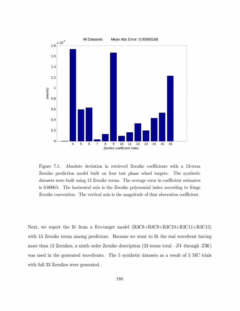
188
Figure 7.1. Absolute deviation in retrieved Zernike coefficients with a 13-term
Zernike prediction model built on four test phase wheel targets. The synthetic
datasets were built using 13 Zernike terms. The average error in coefficient estimates
is 0.0006l. The horizontal axis is the Zernike polynomial index according to fringe
Zernike convention. The vertical axis is the magnitude of that aberration coefficient.
Next, we report the fit from a five-target model (R3C8+R3C9+R3C10+R3C11+R3C15)
with 13 Zernike terms among predictors. Because we want to fit the real wavefront having
more than 13 Zernikes, a ninth order Zernike description (33 terms total – 4Z through 36Z )
was used in the generated wavefronts. The 5 synthetic datasets as a result of 5 MC trials
with full 33 Zernikes were generated.
4 5 6 7 8 9 10 11 12 13 14 15 160
0.2
0.4
0.6
0.8
1
1.2
1.4
1.6
1.8x 10
-3
Zernike coefficient index
(wav
es)
All Datasets Mean Abs Error: 0.00060168
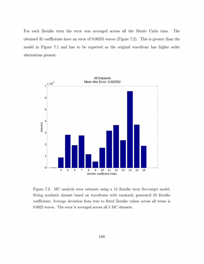
189
For each Zernike term the error was averaged across all the Monte Carlo runs. The
obtained fit coefficients have an error of 0.00255 waves (Figure 7.2). This is greater than the
model in Figure 7.1 and has to be expected as the original wavefront has higher order
aberrations present.
Figure 7.2. MC analysis error estimate using a 13 Zernike term five-target model,
fitting synthetic dataset based on wavefronts with randomly generated 33 Zernike
coefficients. Average deviation from true to fitted Zernike values across all terms is
0.0025 waves. The error is averaged across all 5 MC datasets.
4 5 6 7 8 9 10 11 12 13 14 15 160
1
2
3
4
5
6
7x 10
-3
All DatasetsMean Abs Error: 0.002552
Zernike coefficient index
(wav
es)

190
The individual submodel mean absolute errors (averaged over across all 5 MC datasets) for
R3C8, R3C9, R3C10, R3C11 & R3C15 were 0.00375, 0.00426, 0.0032786, 0.00263, &
0.0027137 waves, respectively. The combined error is smaller than each individual submodel
error.
When using a 5-target model, the Monte Carlo generated wavefronts each were as follows.
Original wavefront RMS OPD were at 0.0174, 0.0187, 0.0147, 0.0162, 0.0117 waves.
Residual wavefront RMS were at 0.0043, 0.0031, 0.0046, 0.0049, 0.0027 waves.
Figure 7.3 below is a typical individual fit (wavefront reconstruction) example from a single
MC iteration. The low order terms fit well. The maximum coefficient deviation is below
4 ml. The mean absolute error is 1.9 ml. The residual wavefront highlights the higher
order aberration present that was not fit.
The model accuracy depends on the choice and the number of test targets. Adding more
targets yields some improvement, with the average residual error further reduced by 0.35
mwaves. We also expect that multi-target models will work better in presence of noise. But
the benefit of adding more targets for accuracy is less practical and is outweighed by the
need for added CPU resources and data collection effort.
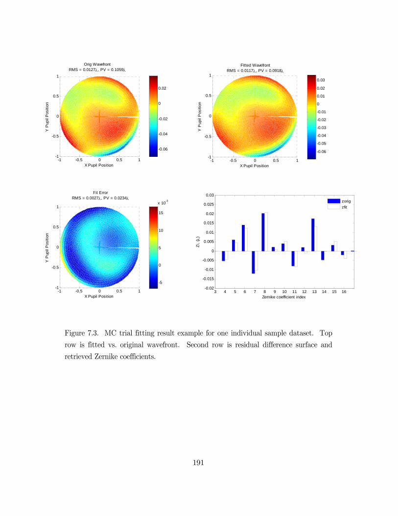
191
Figure 7.3. MC trial fitting result example for one individual sample dataset. Top
row is fitted vs. original wavefront. Second row is residual difference surface and
retrieved Zernike coefficients.
-1 -0.5 0 0.5 1-1
-0.5
0
0.5
1
X Pupil Position
Orig WavefrontRMS = 0.0127, PV = 0.1059
Y P
upil
Pos
ition
-0.06
-0.04
-0.02
0
0.02
-1 -0.5 0 0.5 1-1
-0.5
0
0.5
1
Fitted WavefrontRMS = 0.0117, PV = 0.0918
X Pupil Position
Y P
upil
Pos
ition
-0.06
-0.05
-0.04
-0.03
-0.02
-0.01
0
0.01
0.02
0.03
-1 -0.5 0 0.5 1-1
-0.5
0
0.5
1
Fit ErrorRMS = 0.0027, PV = 0.0234
X Pupil Position
Y P
upil
Pos
ition
-5
0
5
10
15
x 10-3
3 4 5 6 7 8 9 10 11 12 13 14 15 16-0.02
-0.015
-0.01
-0.005
0
0.005
0.01
0.015
0.02
0.025
0.03
Zernike coefficient index
Zi,
( )
zorig
zfit

192
7.2.2 Quality of fit versus aberration order
Of great interest to our study is finding out how a linear model with finite number of
predictors will perform on a real wavefront which theoretically has infinite number of
Zernikes present in lens. Scanner manufacturers typically choose to lump all aberrations
after 36 into residual wavefront but aberrations up to 36 always present in any lens and
their errors contribute significantly to the wavefront RMS.
Wavefront comparison fitting a 13 and 22 Zernike-term models is performed next,
illustrating the model fit result vs. number of terms in model.
Wavefront analysis of two fitted wavefronts is given in Figure 7.4 for the original pupil
defined with 4Z - 36Z aberrations. Fitted wavefront surface using 13 Zernike coefficients
(top left) is compared to the wavefront fitted with 22 Zernike terms (top right). Both
models provide a reasonable fit to the data, as the difference plot between the two
wavefronts (bottom left) shows. The fit differences are mainly in the outer portion of the
pupil, which highlights the need to include high-order Zernike polynomial terms in the
wavefront description. Also in Figure 7.4, a direct comparison for each Zernike coefficient is
made with original wavefront (bottom right). The coefficients predicted with the 22-term
model more closely match the actual coefficients. The 13-term model did not predict the
coefficients as accurately as the 22 model did. The 22-term model error is attributed to
other factors that were not explicitly considered in this model. The cross-talk (§5.2.1)
manifested in the 13-term model result is improved by adding more actual terms with 22-
term model. The residual error is dominated by higher order Zernike coefficients ( 26Z and
up), hence, the surface error is evident in areas around the pupil edge.
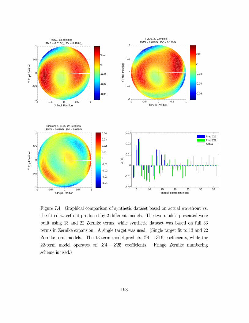
193
Figure 7.4. Graphical comparison of synthetic dataset based on actual wavefront vs.
the fitted wavefront produced by 2 different models. The two models presented were
built using 13 and 22 Zernike terms, while synthetic dataset was based on full 33
terms in Zernike expansion. A single target was used. (Single target fit to 13 and 22
Zernike-term models. The 13-term model predicts 4Z — 16Z coefficients, while the
22-term model operates on 4Z — 25Z coefficients. Fringe Zernike numbering
scheme is used.)
-1 -0.5 0 0.5 1-1
-0.5
0
0.5
1
R3C9, 13 Zernikes RMS = 0.0174, PV = 0.1094
X Pupil Position
Y P
upil
Pos
ition
-0.06
-0.04
-0.02
0
0.02
-1 -0.5 0 0.5 1-1
-0.5
0
0.5
1
X Pupil Position
R3C9, 22 Zernikes RMS = 0.0182, PV = 0.1260
Y P
upil
Pos
ition
-0.06
-0.04
-0.02
0
0.02
-1 -0.5 0 0.5 1-1
-0.5
0
0.5
1
Difference, 13 vs. 22 Zernikes RMS = 0.0107, PV = 0.0890
X Pupil Position
Y P
upil
Pos
ition
-0.04
-0.03
-0.02
-0.01
0
0.01
0.02
0.03
0.04
5 10 15 20 25 30 35-0.02
-0.01
0
0.01
0.02
0.03
Zernike coefficient index
Zi,
( )
Pred Z13
Pred Z22Actual

194
The accuracy that can be gained from a 22-term model is obvious, where the largest error in
the coefficients is 0.004 waves. Using a single target at multiple dose and focus settings is
effective in fitting of additional Zernike terms, including those terms with higher power in
the radial term. The coefficients of certain high order terms are more difficult to fit
compared to others. As power of the radial term in Zernike polynomial is increasing and the
angular frequency is increasing, the shapes of the terms get more complicated to reconstruct
without revising the partial coherence setting or adding more targets to the model. The
optimization effort was focused on fitting all terms, particularly these higher order radial
terms. If we look at Zernike basis functions’ radial component and the frequency
component, using the ordering scheme in Figure 3.4, we see that all these terms are
increasingly difficult to resolve if full image intensity is not available. The range of doses is
needed. The dose is indeed the key factor in the model that helps resolve the offending
terms. The accuracy is expected to further improve when we include a second target. The
goal is to keep the number of targets to a minimum for a manageable data collection cycle.
7.2.3 Single target, 33 Zernikes
It took 53,100 runs to generate the data in order to build this model.
Model prediction result, fitting 33 Zernike coefficients on 3 synthetic datasets is shown in
Figure 7.5. Reported is an average error after 3 Monte Carlo runs against each Zernike
term. The single target (R3C9) model produces a 1.59 mwave error on average across 33
Zernike terms ( 4Z — 36Z ).
The accuracy that can be gained from using a single target with a 33 predictor model is
shown in Figure 7.5, where the largest error in the coefficients is 0.004 waves. It is possible
to achieve a 0.00159 wave error on average, across all Zernike coefficients. Two thirds of the
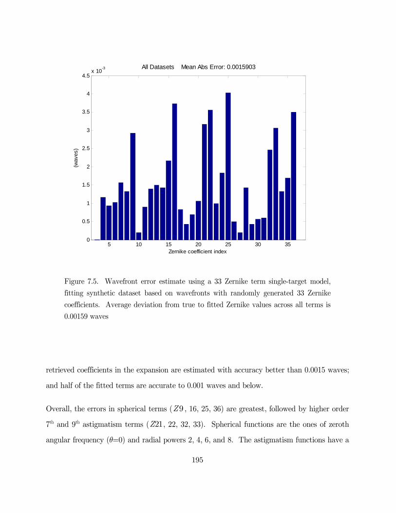
195
Figure 7.5. Wavefront error estimate using a 33 Zernike term single-target model,
fitting synthetic dataset based on wavefronts with randomly generated 33 Zernike
coefficients. Average deviation from true to fitted Zernike values across all terms is
0.00159 waves
retrieved coefficients in the expansion are estimated with accuracy better than 0.0015 waves;
and half of the fitted terms are accurate to 0.001 waves and below.
Overall, the errors in spherical terms ( 9Z , 16, 25, 36) are greatest, followed by higher order
7th and 9th astigmatism terms ( 21Z , 22, 32, 33). Spherical functions are the ones of zeroth
angular frequency (q=0) and radial powers 2, 4, 6, and 8. The astigmatism functions have a
5 10 15 20 25 30 350
0.5
1
1.5
2
2.5
3
3.5
4
4.5x 10
-3 All Datasets Mean Abs Error: 0.0015903
Zernike coefficient index
(wav
es)

196
2q angular dependence and radial powers of 6 and 8. These are all so-called even aberrations
with rotational symmetry (or xy-symmetry) that manifest themselves through-focus. The
coefficients of certain high order terms are more difficult to fit compared to others, including
those terms with higher power in the radial term. As power of the radial term in Zernike
polynomial is increasing and the angular frequency is increasing, the shapes of the terms get
more complicated. The optimization effort was focused on fitting all terms, particularly
these higher order radial terms. The accuracy is expected to further improve when we
include a second target. However, the goal is to keep the number of targets to a minimum
for a manageable data collection cycle.
7.3 Implementation results summary
To validate the regression model and its predictive ability the Monte Carlo method was
applied. Using the approach described in experimental sections (Chapters 5 and 6), multiple
regression models were created that estimate wafer image based on wavefront input. These
models varied in complexity, i.e. the order of the wavefront they operate on and also in the
number of targets they could predict simultaneously. Among the models created were single
and multi-target models supporting wavefronts of varying sets of orders, meaning models
operating on 13, 22, and 33 predictors.
Wavefronts for testing were randomly created using Monte Carlo seeds. Experimental
datasets from these wavefronts were generated using forward calculations in the full rigorous
simulator PROLITH. The optimization approach was then used to produce an estimate of
the original wavefront from the datasets using the regression (high-speed) models.
In the example in §7.2.1 we considered a multi-target model with 13 Zernike terms (plus
dose and focus) as predictors, illustrating the level of accuracy possible in the estimation of
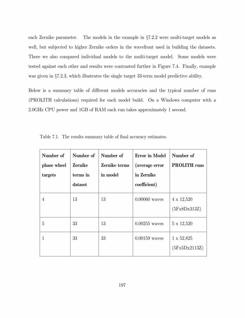
197
each Zernike parameter. The models in the example in §7.2.2 were multi-target models as
well, but subjected to higher Zernike orders in the wavefront used in building the datasets.
There we also compared individual models to the multi-target model. Some models were
tested against each other and results were contrasted further in Figure 7.4. Finally, example
was given in §7.2.3, which illustrates the single target 33-term model predictive ability.
Below is a summary table of different models accuracies and the typical number of runs
(PROLITH calculations) required for each model build. On a Windows computer with a
2.0GHz CPU power and 1GB of RAM each run takes approximately 1 second.
Table 7.1. The results summary table of final accuracy estimates.
Number of
phase wheel
targets
Number of
Zernike
terms in
dataset
Number of
Zernike terms
in model
Error in Model
(average error
in Zernike
coefficient)
Number of
PROLITH runs
4 13 13 0.00060 waves 4 x 12,520
(5Fx8Dx313Z)
5 33 13 0.00255 waves 5 x 12,520
1 33 33 0.00159 waves 1 x 52,825
(5Fx5Dx2113Z)

198
7.4 Discussion
We showed that the method works and discussed efficient estimation of parameters for a
given model. A simple 13-term model based on a single target provides vector estimates
with smallest average mean squared error. It is accurate to 0.6 mwaves. The observed
residual error is smallest when fitting to a low order wavefront (13 terms). The model with
13 terms achieves 2.5 mwave accuracy on a full wavefront (§7.2.1). As expected, models
with 13 terms have been found to be very robust.
Large models are very promising. As shown in §7.2.3, even with 1 target, the 33-term model
is a fully capable model at 1.6 mwaves accuracy. Observed error was strongest about the
spherical aberration group, followed by astigmatism. The greatest challenge was in
retrieving spherical aberration terms. Multiple targets help with spherical (where variations
within the other Zernike groups depend on high orders).
Overall, the models appear to work as desired. Low order Zernike models seem to have
more error than wanted when analyzed with full wavefront. The error went up to 2.5
mwave but is still within goals. It is very encouraging that the high order Zernike model
could fit 33 aberration coefficients with the same error, as this is evidence of well-calibrated
model, and it is possible to achieve the desired accuracy. The more sophisticated the model
is, the more carefully it needs to be calibrated. Shorter models have been built with 4 or 5
targets at a time, but they suffer from accuracy trade-off.
Through focus spherical ( 9Z , 16Z , 25Z ) and high order astigmatism were found to have
lower accuracy compared to other terms due to partial coherence setting of 0.3 being
relatively high.

199
An issue may arise when the actual wavefront contains more orders than those accounted for
by the model (§5.2.2). However, it can be argued that the imaging effects from higher order
Zernike terms being lumped (or their respective errors being redistributed into low orders)
must be very similar. The model verification has been performed to better understand the
capabilities of models of varying complexity.
The results of the Monte Carlo study have validated the chosen regression model versus the
full physical model. These results are promising, suggesting significant improvement in
coefficient estimation when including through dose information. In general, an optimum
convergence is obtained with this approach. In order to keep measurement and simulation
burdens realistic, two paradigms were considered. In one scenario, multiple targets were
used. In a second scenario, a single target was analyzed through dose and focus. The
substantial advantage is seen with multiple targets.
200
8. Conclusions
Aberration monitoring represents a complex problem in modern microlithography. The
imaging tools are performing to the diffraction resolution limit as close as possible, with
aberrations significantly influencing the image formation. It is difficult to measure
aberrations once the lens has been assembled inside the tool. Various existing methods all
have their drawbacks and research continues to be of significant interest. The proposed
method of computer assisted analysis of images produced by phase wheel targets has been
developed and demonstrated. This method differs from most other aberration methods in
that it can be used after the lens has been installed in the tool while still providing high
sensitivity and accuracy.
The proposed method consists of a carefully optimized set of test targets combined with
computer assisted data analysis and fitting method. The fast regression model combines
accuracy of the physical model and speed at the cost of being limited to the targets selected
in their subspaces. The approach is predicated on the ability to parameterize the outputs—
the experimentally observed two-dimensional images. The parameterization scheme was
developed and tested on a large number of images produced with several types of scanning
electron microscopes. The image processing algorithm is flexible and has been fine tuned to
account for the differences in image capturing techniques.
201
The core of the method is computer optimization of the imaging properties of the
lithography system given a set of observed images. A nonlinear optimization scheme was
used to minimize the difference between the simulated and the parameterized observed wafer
data, and the approach converged to solutions on multiple sets of experimental data.
Lithographic processing has hundreds of parameters and analyzing and capturing all
interactions is a daunting task. Accurate models for image response were constructed and
their use for aberration retrieval has been demonstrated. The fact that the method was
successful in achieving the goal of building a polynomial model of such a complex system and
a problem that handles shapes of arbitrary complexity is a step forward in building a unified
system. The model is a tremendous learning instrument of how different aberrations impact
the image shapes. This model and methodology has potential for much wider application.
The key to the highest accuracy is a well calibrated physical model. Steps that allow doing
such model calibration very efficiently were developed.
The data approach was tested both on aerial images at the wafer level and on latent resist
images. Feasibility was shown with intensity images and with wafer images. This was one
milestone in development of the method. Another milestone was learning on the image
processing of SEM images.
Accuracy and repeatability of the aberration retrieval was studied using a Monte Carlo
approach where pre-generated datasets based on a random set of system Zernike parameters
took the place of the experimental data and the fitting results were compared to the original
true set of Zernikes. The final chapter (§7) applies the procedure to a synthetic Monte Carlo
example; its numerical results are encouraging. Zernike recovery capability appears to have
satisfied the goal set out in the program inception and therefore was successful.
202
The specific milestones covered in Chapters 4 through 7 were as follows.
In §4, an efficient target design capable of accurate phase measurement is demonstrated.
The design is relatively simple making this test suitable for a broad range of measurement
applications and wavelengths. In §4.2, general analysis of the method is presented. The
method combines some of the good qualities such as speed and the possibility of qualitative
information due to sensitivity to certain aberration types. The method generally involves a
combination of both computation and visualization. The phase wheel aberration monitor is
a useful tool for estimating and correcting the phase errors in the projection tool setup.
Since the test also establishes unique associations between the various aberrations, the phase
wheel is a good choice as a monitoring tool capable of providing rapid feedback. Phase
aberrations may be inferred directly from the image data. Targets can be included on all
PSMs as aberration monitors. Qualitative and quantitative analysis is possible, with small
aberration effects becoming obvious. In §4.3.1, several improvements on the edge extraction
algorithm have been realized, allowing more reliable, robust detection for a variety of SEM
tools and increased accuracy.
In §5, the target was applied to testing of aberrations in 157 and 193 nm projection
lithography systems. Simulation results using synthetic images show that Zernike aberration
coefficients can be recovered from intensity information, given appropriate target choice.
The results indicate that it is feasible to use the phase wheel aberration monitor for
characterizing the high order Zernike space (33 terms). The model has been validated to
provide a high sensitivity (wave errors at l193/100) as well as high accuracy. This
performance compares favorably with other methods. In the noiseless case, the fitting error
as predicted is less than 0.01%, which is below the typical noise level of any current system.
The method is extendible to incorporate resist imaging into the model, and is capable of
203
using SEM images in resist for fitting the aberrations. In §5.2.2, an approach for fitting
aberrations based on wafer-level data has been developed, a significant extension to the
aerial-image based method presented in §5.2.1.
In §6, a technique for automated aberration extraction has been further developed. The
fitting algorithm includes the nonlinear optimization of the fit parameters. (Nonlinear
optimization proved useful for fitting a variety of targets.) The method has been optimized
using a compact response surface model in conjunction with optical lithography simulation.
A stand-alone aberration analysis application has been developed in MATLAB that supports
the entire phase wheel data analysis process and provides a flexible environment for the
large-scale problems modeled. Computational efficiency of the approach has been a
paramount goal, and a less than one hour convergence time has been achieved. In §§6.3–6.5,
algorithms for fitting empirical data have been identified, tested, and shown to produce
1-mwave average accuracy across 35 aberration terms. Phase wheel targets provide high
sensitivity and yield good results. The example for the method was given, characterizing a
typical 193 nm lens.
In §7, we have presented detailed accuracy analysis of the phase wheel aberration extraction
method. The wavefronts have been fit using up to 36 Zernike terms, incorporating image
processing, calibration, edge extraction and wavefront surface fitting. The phase wheel
aberration extraction method has been demonstrated as viable and practical for 1-mwave
accuracy. Better than 0.7 nm (0.0035 l) of accuracy with less than 0.4 nm (0.002 l) of
repeatability at 193 nm in photoresist has been achieved.

204
References
Born, M., & Wolf, E. (1997). Principles of optics : electromagnetic theory of propagation, interference and diffraction of light (6th corrected ed.). Cambridge, UK ; New York: Cambridge University Press.
Born, M., & Wolf, E. (1999). Principles of optics : electromagnetic theory of propagation, interference and diffraction of light (7th expanded ed.). Cambridge ; New York: Cambridge University Press.
Bossung, J. W. (1977). Projection printing characterization. Developments in Semiconductor Microlithography II, SPIE Proceedings. 80.
Box, G. E. P., & Behnken, D. W. (1960). Some new three level designs for the study of quantitative variables. Technometrics, 2(4), 455-475.
Braat, J., & Janssen, A. J. E. M. (1999). Improved Ronchi test with extended source. J. Opt. Soc. Am. A, 16(1), 131-140.
Braat, J. J. M., Dirksen, P., Janssen, A. J. E. M., & van de Nes, A. S. (2003). Extended Nijboer-Zernike representation of the vector field in the focal region of an aberrated high-aperture optical system. J. Opt. Soc. Am. A, 20(12), 2281-2292.
Brunner, T. A., Martin, A. L., Martino, R. M., Ausschnitt, C. P., Newman, T. H., & Hibbs, M. S. (1994). Quantitative stepper metrology using the focus monitor test mask. Optical/Laser Microlithography VII. San Jose, CA, USA: SPIE. 541-549.
Cornejo-Rodriquez, A. (1992). Ronchi test. In D. Malacara (Ed.), Optical shop testing. New York: Wiley, p. 321-66.
Dai, G.-m. (2006). Zernike aberration coefficients transformed to and from Fourier series coefficients for wavefront representation. Optics Letters, 31(4), 501-503.
Dirksen, P., Braat, J., Janssen, A. J. E. M., & Juffermans, C. (2003a). Aberration retrieval using the extended Nijboer-Zernike approach. Journal of Microlithography, Microfabrication, and Microsystems, 2(1), 61-68.
Dirksen, P., Braat, J. J., Janssen, A. J., & Leeuwestein, A. (2005). Aberration retrieval for high-NA optical systems using the extended Nijboer-Zernike theory. Optical Microlithography XVIII. San Jose, CA, USA: SPIE. 262-273.

205
Dirksen, P., Braat, J. J. M., M., J. A. J. E., Juffermans, C. A. H., & Leeuwestein, A. (2003b). Experimental determination of lens aberrations from the intensity point-spread function in the focal region. Optical Microlithography XVI. Santa Clara, CA, USA: SPIE. 1-10.
Dirksen, P., Juffermans, C. A. H., Engelen, A., De Bisschop, P., & Muellerke, H. (2000). Impact of high-order aberrations on the performance of the aberration monitor. Optical Microlithography XIII. Santa Clara, CA, USA: SPIE. 9-17.
Dirksen, P., Juffermans, C. A. H., Pellens, R. J. M., Maenhoudt, M., & De Bisschop, P. (1999). Novel aberration monitor for optical lithography. Optical Microlithography XII. Santa Clara, CA, USA: SPIE. 77-86.
Draper, N. R., & Smith, H. (1998). Applied regression analysis (3rd ed.). New York: Wiley.
Farrar, N. R., Smith, A. H., Busath, D. R., & Taitano, D. (2000). In-situ measurement of lens aberrations. Optical Microlithography XIII. Santa Clara, CA, USA: SPIE. 18-29.
Flagello, D. G., de Klerk, J., Davies, G., Rogoff, R., Geh, B., Arnz, M., Wegmann, U., & Kraemer, M. (1997). Toward a comprehensive control of full-field image quality in optical photolithography. Optical Microlithography X. Santa Clara, CA, USA: SPIE. 672-685.
Flagello, D. G., & Geh, B. (1998). The influence of lens aberrations in lithography. Microlithography World. USA: PennWell Publishing Company, 11-17.
Foucault, L. (1859). Memoire sur la construction des telescopes en verre argente. Annales de l'Observatoire de Paris, 5, 197-237.
Ghozeil, I. (1992). Hartmann and other screen tests. In D. Malacara (Ed.), Optical shop testing. New York: Wiley, p. 367-96.
Goldberg, K. A., Naulleau, P., Bokor, J., Chapman, H. N., & Barty, A. (2002). Testing extreme ultraviolet optics with visible-light and extreme ultraviolet interferometry. Journal of Vacuum Science & Technology B, 20(6), 2834-2839.
Gonsalves, R. A. (1982). Phase retrieval and diversity in adaptive optics. Optical Engineering, 21, 829-832.
Gonzalez, R. C., & Woods, R. E. (2002). Digital image processing (2nd ed.). Upper Saddle River, N.J.: Prentice Hall.
Gonzalez, R. C., Woods, R. E., & Eddins, S. L. (2004). Digital Image processing using MATLAB. Upper Saddle River, NJ: Pearson/Prentice Hall.
Goodman, J. W. (1996). Introduction to Fourier optics (2nd ed.). New York: McGraw-Hill.
Goodman, J. W. (2000). Statistical optics (Wiley classics library ed.). New York: Wiley.
Greivenkamp, J. E., & Bruning, J. H. (1992). Phase shifting interferometry. In D. Malacara (Ed.), Optical shop testing. New York: Wiley, p. 501-98.
206
Hartmann, J. (1904). Objektuvuntersuchungen. Zeitschrift für Instrumentenkunde, 24(1-2), 1-47.
Hegeman, P., Christmann, X., Visser, M., & Braat, J. (2001). Experimental study of a shearing interferometer concept for at-wavelength characterization of extreme-ultraviolet optics. Appl. Opt., 40(25), 4526-4533.
Herrmann, J. (1981). Cross coupling and aliasing in modal wave-front estimation. J. Opt. Soc. Am., 71(8), 989.
Hopkins, H. H. (1953). On the Diffraction Theory of Optical Images. Proceedings of the Royal Society of London. Series A, Mathematical and Physical Sciences, 217(1130), 408-432.
Intel.com (2010) Intel Itanium® 9300 Processor Raises Bar for Scalable, Resilient Mission-Critical Computing, accessed 21 April 2010, [available at http://www.intel.com/pressroom/archive/releases/20100208comp.htm].
ITRS (2009). 2009 EDITION : LITHOGRAPHY. In International Roadmap Committee (Ed.), INTERNATIONAL TECHNOLOGY ROADMAP FOR SEMICONDUCTORS, http://public.itrs.net/reports.html.
Janssen, A. J. E. M. (2002). Extended Nijboer-Zernike approach for the computation of optical point-spread functions. J. Opt. Soc. Am. A, 19(5), 849-857.
Kaise, K., Tsukakoshi, T., & Hayashi, T. (2001). Method for the measurement of aberration of optical projection system. US Patent No. 6,296,977. Nikon Corporation.
Kass, M., Witkin, A., & Terzopoulos, D. (1987). Snakes: active contour models. Proceedings - First International Conference on Computer Vision. London, Engl: IEEE. 259-268.
Kim, J.-C., & Shannon, R. R. (1987). Catalog of Zernike polynomials. In R. R. Shannon, & J. C. Wyant (Eds.), Applied Optics and Optical Engineering. New York: Academic Press, p. 193-221.
Kirk, J. P., & Progler, C. J. (1999). Application of blazed gratings for determination of equivalent primary azimuthal aberrations. Optical Microlithography XII. Santa Clara, CA, USA: SPIE. 70-76.
KLA-Tencor (2007). PROLITH/9.3.2.2. © 2007 KLA-Tencor Corp., Milpitas, CA, USA. http://www.kla-tencor.com/lithography-modeling/chip-prolith.html.
Levenson, M. D., Viswanathan, N. S., & Simpson, R. A. (1982). Improving resolution in photolithography with a phase-shifting mask. Electron Devices, IEEE Transactions on, 29(12), 1828-1836.
Li, C., Xu, C., Gui, C., & Fox, M. D. (2005). Level set evolution without re-initialization: a new variational formulation. Computer Vision and Pattern Recognition 2005, IEEE Computer Society Conference on CVPR. 430-436.

207
Loomis, J. (1978). A computer program for analysis of interferometric data. Optical Interferograms—Reduction and Interpretation. Philadelphia, PA: American Society for Testing and Materials. 71-86.
Mack, C. A., & Byers, J. D. (2003). New model for focus-exposure data analysis. Metrology, Inspection, and Process Control for Microlithography XVII. Santa Clara, CA, USA: SPIE. 396-405.
Mack, C. A., Jug, S., & Legband, D. A. (1999). Data analysis for photolithography. Metrology, Inspection, and Process Control for Microlithography XIII. Santa Clara, CA, USA: SPIE. 415-434.
Mahajan, V. N. (1991). Aberration theory made simple. Bellingham, Wash., USA: SPIE Optical Engineering Press.
Malacara, D. (1992). Optical shop testing (2nd ed.). New York: Wiley.
Malacara, D., & DeVore, S. L. (1992). Interferogram evaluation and wavefront fitting. In D. Malacara (Ed.), Optical shop testing. New York: Wiley, p. 455-99.
MathWorks (2007). MATLAB® 7.4 (R2007a). © 2007 The MathWorks Inc., Natick, MA, USA. http://www.mathworks.com.
Medecki, H., Tejnil, E., Goldberg, K. A., & Bokor, J. (1996). Phase-shifting point diffraction interferometer. Opt. Lett., 21(19), 1526.
Moers, M. H. P., van der Laan, H., Zellenrath, M., de Boeij, W., Beaudry, N. A., Cummings, K. D., van Zwol, A., Brecht, A., & Willekers, R. (2001). Application of the aberration ring test (ARTEMIS) to determine lens quality and predict its lithographic performance. Optical Microlithography XIV. Santa Clara, CA, USA: SPIE. 1379-1387.
Moore, G. E. (1965). Cramming more components onto integrated circuits. Electronics, 38(8).
Naulleau, P., Goldberg, K. A., Anderson, E. H., Batson, P., Denham, P. E., Jackson, K. H., Gullikson, E. M., Rekawa, S., & Bokor, J. (2001). At-wavelength characterization of the extreme ultraviolet Engineering Test Stand Set-2 optic. Journal of Vacuum Science & Technology B, 19(6), 2396-2400.
Naulleau, P. P., & Goldberg, K. A. (1999). Dual-domain point diffraction interferometer. Appl. Opt., 38(16), 3523-3533.
Neureuther, A. R., Adam, K., Robins, G. C., & Gennari, F. E. (2006). Characterizing aberrations in an imaging lens and applications to visual testing and integrated circuit mask analysis. US Patent No. 7,030,997. The Regents of the University of California.
Nijboer, B. R. A. (1942). The diffraction theory of aberrations, Thesis, University of Groningen : Netherlands.
Nijboer, B. R. A. (1943). The diffraction theory of optical aberrations: Part I: General discussion of the geometrical aberrations. Physica, 10, 679-692.
208
Noll, R. J. (1976). Zernike polynomials and atmospheric turbulence. J. Opt. Soc. Am., 66(3), 207-211.
Ojeda-Castañeda, J. (1992). Foucault, wire, and phase modulation tests. In D. Malacara (Ed.), Optical shop testing. New York: Wiley, p. 265-320.
Partlo, W. N., Fields, C. H., & Oldham, W. G. (1993). Direct aerial image measurement as a method of testing high numerical aperture microlithographic lenses. Journal of Vacuum Science Technology B: Microelectronics and Nanometer Structures, 11, 2686-2691.
Press, W. H. (2007). Numerical recipes : the art of scientific computing (3rd ed.). Cambridge, UK ; New York: Cambridge University Press.
Robins, G., Adam, K., & Neureuther, A. (2002). Measuring optical image aberrations with pattern and probe based targets. Journal of Vacuum Science & Technology B: Microelectronics and Nanometer Structures, 20(1), 338-343.
Robins, G., & Neureuther, A. (2003a). Pattern and probe-based aberration monitors for the human eye. Journal of Vacuum Science & Technology B, 21(6), 2922-2925.
Robins, G. C. (2005). Interferometric pattern and probe-based aberration monitors, Thesis, University of California, Berkeley.
Robins, G. C., Dusa, M., Geh, B., & Neureuther, A. R. (2003). Interferometric-probe aberration monitors: aerial image and in-resist performance. 23rd Annual BACUS Symposium on Photomask Technology. Monterey, CA, USA: SPIE. 309-317.
Robins, G. C., & Neureuther, A. R. (2003b). Experimental assessment of pattern and probe-based aberration monitors. Optical Microlithography XVI. Santa Clara, CA, USA: SPIE. 1420-1431.
Robins, G. C., & Neureuther, A. R. (2005). Are pattern and probe aberration monitors ready for prime time? Optical Microlithography XVIII. San Jose, CA, USA: SPIE. 1704-1715.
Robins, G. C., Neureuther, A. R., Dusa, M., & Kye, J. (2004). Interferometric-probe aberration monitor performance in the production environment. Optical Microlithography XVII. Santa Clara, CA, USA: SPIE. 1971-1982.
Roddier, F., & Roddier, C. (1991). Wavefront reconstruction using iterative Fourier transforms. Appl. Opt., 30(11), 1325-1327.
Ronchi, V. (1964). Forty Years of History of a Grating Interferometer. Appl. Opt., 3(4), 437-451.
Saleh, B. E. A. (1979). Optical Bilinear Transformations: General Properties. Optica Acta: International Journal of Optics, 26(6), 777 - 799.
SAS (2007). JMP® 7.0.1 software. Copyright © 2007, SAS Institute Inc., Cary, NC, USA. http://www.jmp.com.

209
Schuster, K.-H., & Epple, A. (2006). Lithographic objective having a first lens group including only lenses having a positive refractive power. US Patent No. 7,023,627 B2. Carl Zeiss SMT AG.
Schwider, J. (1981). Single sideband Ronchi test. Appl. Opt., 20(15), 2635-2642.
Seong, N., Yeo, G., Cho, H., & Moon, J.-T. (2000). Measurement of lens aberration by using in-situ interferometer and classification of lens for correct application. Optical Microlithography XIII. Santa Clara, CA, USA: SPIE. 30-39.
Shack, R. V., & Platt, B. C. (1971). Production and use of a lenticular Hartmann screen. J. Opt. Soc. Am., 61, 656.
Singer, W., Totzek, M., & Gross, H. (2005). Handbook of Optical Systems : Physical Image Formation. Weinheim: Wiley-VCH.
Smith, A. H., McArthur, B. B., & Hunter, R. O. J. (1999). Apparatus method of measurement and method of data analysis for correction of optical system. US Patent No. 5,978,085. Litel Instruments.
Smith, B. W. (1999). Variations to the influence of lens aberration invoked with PSM and OAI. Optical Microlithography XII. Santa Clara, CA, USA: SPIE. 330-346.
Sueda, T., & Yoshii, M. (1987). Aberration measuring method. US Patent No. 4,641,962. Canon Kabushiki Kaisha.
Suzuki, K., & Smith, B. W. (Eds.) (2007). Microlithography : science and technology (2nd ed.). Boca Raton: CRC Press.
Tao, P., Balijepalli, A., Gupta, S. K., & LeBrun, T. W. (2006). Algorithms for on-line monitoring of components in an optical tweezers-based assembly cell. Proceedings of the ASME Design Engineering Technical Conference. New York, NY, USA: American Society of Mechanical Engineers. 13.
Taylor, H. D. (1896). On the adjustment and testing of telescopic objectives (2nd ed.). York: T. Cooke & Sons.
Töpler, A. (1864). Beobachtungen nach einer neuen optischen methode. Bonn: Maximilian Cohen und Sohn.
van de Kerkhof, M. A., de Boeij, W., Kok, H., Silova, M., Baselmans, J., & Hemerik, M. (2004). Full optical column characterization of DUV lithographic projection tools. Optical Microlithography XVII. Santa Clara, CA, USA: SPIE. 1960-1970.
van der Laan, H., Dierichs, M., van Greevenbroek, H., McCoo, E., Stoffels, F., Pongers, R., & Willekers, R. (2001). Aerial image measurement methods for fast aberration set-up and illumination pupil verification. Optical Microlithography XIV. Santa Clara, CA, USA: SPIE. 394-407.
van der Laan, H., & Moers, M. H. (2005). Method of measuring aberration in an optical imaging system. US Patent No. 6,897,947. ASML Netherlands B.V.
210
Venkataraman, P., & Smith, B. W. (2000). Aberrations of steppers using phase-shifting point diffraction interferometry. Optical Microlithography XIII. Santa Clara, CA, USA: SPIE. 1245-1249.
Williamson, D. M. (1994). The elusive diffraction limit. OSA proceedings on extreme ultraviolet lithography. Monterey, CA, USA: Optical Society of America. 68-86.
Williamson, D. M. (2005). Remaining challenges in microlithographic optical design. Current Developments in Lens Design and Optical Engineering VI. San Diego, CA, USA: SPIE. 58740N-12.
Wolter, H. (1956). Schlieren-, Phasenkontrast- und Lichtschnittverfahren. In S. Flügge (Ed.), Handbuch der Physik. Berlin: Springer, 555-645.
Wyant, J. C. (1973). Double frequency grating lateral shear interferometer. Appl. Opt., 12(9), 2057-2060.
Wyant, J. C., & Creath, K. (1992). Basic wavefront aberration theory for optical metrology. In R. R. Shannon, & J. C. Wyant (Eds.), Applied Optics and Optical Engineering. New York: Academic Press, p. 1-53.
Yeung, M. S. (2000). Measurement of wave-front aberrations in high-resolution optical lithographic systems from printed photoresist patterns. Semiconductor Manufacturing, IEEE Transactions on, 13(1), 24-33.
Zernike, v. F. (1934). Beugungstheorie des schneidenver-fahrens und seiner verbesserten form, der phasenkontrastmethode. Physica, 1(7-12), 689-704.