measuring credit risk in a large banking system: econometric modeling and empirics - andre lucas,...
TRANSCRIPT
Measuring credit risk in a large banking
system: econometric modeling and
empirics*
SYstemic Risk TOmography:
Signals, Measurements, Transmission
Channels, and Policy Interventions
F.E.B.S., 3rd annual conference
June 7, 2013
Andre Lucas, Bernd Schwaab, Xin ZhangVU University Amsterdam / ECB / Riksbank
*: Not necessarily the views of ECB or Sveriges Riksbank

Intro Model Empirics Conclusion
Outline
Intro
Model
Empirics
Conclusion
1 / 37

Intro Model Empirics Conclusion
Motivation
Since 2007, financial stability surveillance and assessment have become
key priorities in central banks, in addition to monetary policy.
Prudential mandate entails a high-dimensional problem. For example,
FDIC oversees > 7000 U.S. banks. SSM ≈ 130 + 5800 European banks.
Objective: Develop framework to give model-based answers to what is
financial sector joint tail risk? Tail risk conditional on one default?
Useful for counterparty credit risk management, and assessing the impact
of monetary policy measures on euro area financial sector (tail) risk.
2 / 37

Intro Model Empirics Conclusion
Contributions
We develop a novel non-Gaussian, high-dimensional framework to infer
conditional and joint measures of financial sector risk.
Derive a conditional LLN to compute risk measures without simulation.
Based on a multivariate skewed–t density, with tv volatilities and
dependence. Fits large cross-section due to a parsimonious factor
structure.
Model is sufficiently flexible for frequent re-calibration to market data.
Works well with unbalanced data/missing values.
Application to euro area financial firms from 1999M1 to 2013M3.
3 / 37

Intro Model Empirics Conclusion
Two problems...and answers
P1: Financial sector comprises many firms. Joint risk assessment is a
high-dimensional & non-Gaussian problem.
A1: GHST handles non-Gaussian features and DECO the large cross
section. The cLLN facilitates computation of joint and conditional risk
measures.
P2: Stress dependence is time-varying and not directly observed. In bad
times, both uncertainty/volatility and dependence increase. Time varying
parameters required.
A2: Either a non-Gaussian state space model, using simulation methods,
or a observation driven/GAS model, using standard Maximum Likelihood.
Thus, high-dimensional non-normal time-varying parameter model, with
unobserved factors.
4 / 37
Intro Model Empirics Conclusion
Literature
1. Portfolio credit risk and loss asymptotics: Vasicek (1977), Lucas,
Straetmans, Spreij, Klaasen (2001), Gordy (2003), Koopman, Lucas, Schwaab
(2011, 2012).
2. Market risk methods (volatility & NG dependence): Engle
(2002), Demarta and McNeil (2005), Creal, Koopman, and Lucas (2011),
Zhang, Creal, Koopman, Lucas (2011).
3. Observation-driven time-varying parameter models: Creal,
Koopman, and Lucas (2013), Creal, Schwaab, Koopman, Lucas (2013), Harvey
(2012), Patton and Oh (2013).
4. Financial sector risk assessment/systemic risk: Most related are
Hartmann, Straetman, de Vries (2005), Malz (2012), Suh (2012), and Black,
Correa, Huang, Zhou (2012).
5 / 37

Intro Model Empirics Conclusion
Market risk - credit risk link
In a Merton (1974) model for i = 1, 2 firms,
dV i,t = Vi,t· (µidt+ σidWi,t) ,
yi,t = log (V i,t/V i,t−1) ∼ N(µi−σ2i /2, σ
2i ),
where Vi,t is the asset value firm i at time t, and dW1,tW2,t = ρdt.
In a Levy-driven model (Bibby and Sorensen (2001)),
dV i,t =1
2v(Vi,t) [log(f(Vi,t)v(Vi,t))]
′dt+
√v(Vi,t)dWi,t,
yi,t = log (V i,t/V i,t−1) ∼ GHST(σ2i , γi, υ),
where v(Vi,t) and f(Vi,t) are real-valued functions.
6 / 37

Intro Model Empirics Conclusion
The GH (skewed t) copula model
Firm defaults iff its log asset value (yit) falls below a threshold (y∗it),where
yit = (ςt − µς)Litγ +√ςtLitεt, i = 1, ..., n,
εt ∼N(0, In) is a vector of risk factors,
Lit contains risk factor loadings, γ ∈ Rn determines skewness,
ςt ∼ IG(ν2 ,ν2 ) is an additional risk factor.
A default occurs with probability pit, where
pit = Pr[yit < y∗it] = Fit(y∗it) ⇔ y∗it = F−1it (pit),
where Fit is the GHST-CDF of yit.
Focus on conditional probabilities Pr[yit < y∗it|yjt < y∗jt], i 6= j, ...
7 / 37

Intro Model Empirics Conclusion
A factor copula model
Consider a two-factor model with common factor κt ∼N(0, 1), common
tail risk factor ςt ∼ IG(ν2 ,ν2 ), and idiosyncratic εt ∼N(0, IN ),
yit = (ςt − µς)γit +√ςtzit, i = 1, ..., N.
zit = ηitκt + λitεit,
where γit = Litγ, E[ςt] = µς and Var[ςt] = σ2ς .
λit =√
1− ρ2it, and ηit=ρit.
Remark: vector ηt∈ RNx1and matrix Λt = diag(λit)∈ RNxN are
functions of ρt (to be estimated later).
8 / 37
Intro Model Empirics Conclusion
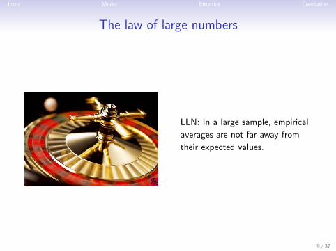
The law of large numbers
LLN: In a large sample, empirical
averages are not far away from
their expected values.
9 / 37

Intro Model Empirics Conclusion
The conditional Law of Large Numbers (1)
The portfolio default fraction at time t is
cN,t=1
N
N∑i=1
1{yi,t< y∗i,t}.
As 1{yi,t< y∗i,t|κt, ςt} are conditionally independent, as N →∞,
cN,t ≈1
N
N∑i=1
E[1{yi,t < y∗i,t|κt, ςt}
]=
1
N
N∑i=1
Pr(yi,t < y∗i,t|κt, ςt
):= CN,t.
10 / 37

Intro Model Empirics Conclusion
The conditional Law of Large Numbers (2)
Two remarks:
• CN,t= 1N
∑Ni=1 Pr
(yi,t < y∗i,t|κt, ςt
)is random because κt, ςt are
random, not because of εt or yi,t.
•
Pr(yi,t < y∗i,t|κt, ςt
)= Φ
((y∗i,t+µςγit−ςtγit)/
√ςt−ηi,tκt
λt
∣∣∣∣κt, ςt) ,where Φ(·) denotes the standard normal CDF.
Given this, a joint tail risk measure (TRMt) is
pt= Pr (CN,t(κt, ςt) > c),
i.e. the probability that the default rate in the portfolio exceeds a fixed
fraction c ∈ [0, 1].
11 / 37

Intro Model Empirics Conclusion
The conditional Law of Large Numbers (3)
CN,t(κt, ςt) is monotonically decreasing in κt for any fixed ςt.
We use this to efficiently compute threshold levels κ∗t,N (c, ς) for each
value of ς by solving CN,t(κ∗t,N (c, ς), ς) ≡ c.
As a result, we can compute the joint tail risk measure (TRMt) very
quickly based on 1-dimensional numerical integration
pt= Pr(CN,t > c) =
∫Pr (κt< κ∗t,N (c, ςt))p(ςt)dςt.
This is a cause for celebration: works within seconds!
12 / 37

Intro Model Empirics Conclusion
The conditional Law of Large Numbers (4)A systemic influence measure (SIMi,t) is given by
Pr (C(−i)N−1,t> c(−i)|yi,t< y∗i,t)
= p−1it Pr(C(−i)N−1,t > c(−i), yi,t < y∗i,t)
= p−1it
∫Pr (κt< κ∗N−1,t(c
(−i), ςt), yi,t < y∗i,t|ςt)p(ςt)dςt
= p−1it
∫Φ2
(κ∗N−1,t(c
(−i), ςt), z∗i,t(·); ηi,t
)p(ςt)dςt,
where c(−i) is a fixed fraction in the portfolio abstracting from firm i,and z∗i,t(y
∗i,t, ςt) = (y∗i,t − (ςt − µς)γi,t)/
√ςt.
Remark: This is close to Hartmann, Straetman, de Vries (2005)’s Multivariate
Extreme Spillovers; but now time-varying at a high frequency.
13 / 37

Intro Model Empirics Conclusion
The conditional Law of Large Numbers (5)
Two final remarks:
1. “Connectedness” := 1N
∑Ni=1SIMi,t
2. SIMi,t without tail risk factor, only common factor exposure
= p−1it Pr(κt < κ∗t,N (c(−i), ςt), yi,t < y∗i,t|ςt)∣∣∣ςt≡1
The difference to full SIMi,t is dependence in excess of what is
implied by common factor exposure.
14 / 37
Intro Model Empirics Conclusion
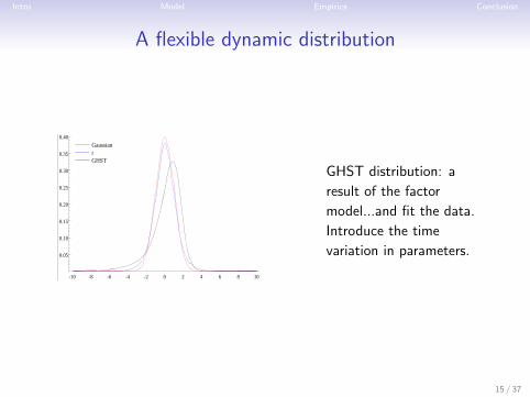
A flexible dynamic distribution
C:\RESEARCH\StabilityMeasure\TexAndOthers\Tex\Presentations\MySlides\graphics\DensGH.eps 12/10/13 17:07:58
Page: 1 of 1
Gaussian t GHST
-10 -8 -6 -4 -2 0 2 4 6 8 10
0.05
0.10
0.15
0.20
0.25
0.30
0.35
0.40
Gaussian t GHST
GHST distribution: a
result of the factor
model...and fit the data.
Introduce the time
variation in parameters.
15 / 37

Intro Model Empirics Conclusion
The dynamic GHST distribution
The GHST pdf nests symmetric-t and normal.
p(yt; ·) =υυ2 21−
υ+n2
Γ(υ2
)πn2
∣∣∣Σt
∣∣∣ 12 ·Kυ+n
2
(√d(yt) · (γ
′γ)
)eγ′L−1t (yt−µt)
(d(yt) · (γ
′γ))−υ+n
4 d(yt)υ+n2
,
where ...
d(yt) = υ + (yt−µt)′Σ−1t (yt−µt),
µt = −υ/(υ − 2) Ltγ,
Σt = LtL′t.
16 / 37

Intro Model Empirics Conclusion
Time varying parameters
A score-driven model ...
Σt = DtRtDt
= Dt(f t)Rt(f t)Dt(f t)
ft+1 = ω+∑p−1
i=0Aist−i+
∑q−1
j=0Bjft−j ,
where st = St∇t is the scaled score
∇t = ∂ ln p(yt; Σ(f t), γ, υ)/∂f tSt = Et−1[∇t∇
′t|yt−1, yt−2, ...]
−1scaling matrix.
See CKL (JAE 2013) for overview and BKL (2012) for stationarity
discussion.
17 / 37

Intro Model Empirics Conclusion
Impact curve: robust to outliers
Figure 1: News impact curve under the Student t score-based conditional variancemodel
−4 −2 0 2 4
05
1015
y
w[v
](y)
y2ν=∞ν=10ν=4
3.2 Model for the conditional copula density function
All assets considered here are major US deposit banks. For such a homogeneous
group of assets, it is reasonable to assume that the correlation parameter in the
copula density function is the same for all pairs of stocks. This so-called “dynamic
equicorrelation parameter” has been extensively studied by Engle and Kelly (2012),
under the assumption that there are no shifts in the unconditional equicorrelation.
In our application on financial institutions, this assumption is likely to be violated.
Because of the interconnectedness between financial institutions, episodes of high
systemic risk are characterized by dramatic changes in the volatility and correlations
of financial institutions. See e.g. the recent empirical evidence in Leonidas and
Italo de Paula (2011) and the review in Section 2. Ang and Chen (2002) find that
10
18 / 37
Intro Model Empirics Conclusion
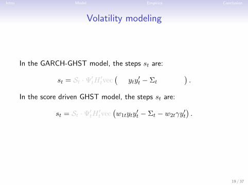
Volatility modeling
In the GARCH-GHST model, the steps st are:
st = St ·Ψ′tH ′tvec(
yty′t − Σt
).
In the score driven GHST model, the steps st are:
st = St ·Ψ′tH ′tvec(w1tyty
′t − Σt − w2tγy
′t
).
19 / 37

Intro Model Empirics Conclusion
Volatility modeling: a comparison
C:\RESEARCH\First Paper\Mphil\2010GASGHST\MGASGHSTFinal\FourSeries\Output\ForSoFiE\VolCompare.gwg 06/13/11 18:09:43
Page: 1 of 1
2002 2003 2004 2005 2006
0.01
0.02
0.03
0.04
0.05
0.06
0.07DCC-GHST Volatility: 03/01/1989 to 01/01/2010
Coca-Cola Merck
IBM JP Morgan
2002 2003 2004 2005 2006
0.01
0.02
0.03
0.04
0.05
0.06
0.07DGH-GHST Volatility: 03/01/1989 to 01/01/2010
Coca-Cola Merck
IBM JP Morgan
20 / 37
Intro Model Empirics Conclusion
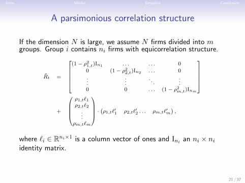
A parsimonious correlation structure
If the dimension N is large, we assume N firms divided into mgroups. Group i contains ni firms with equicorrelation structure.
Rt =
(1− ρ21,t)In1 . . . . . . 0
0 (1− ρ22,t)In2 . . . 0
......
. . ....
0 0 . . . (1− ρ2m,t)Inm
+
ρ1,t`1ρ2,t`2
...ρm,t`m
· (ρ1,t`′1 ρ2,t`′2 . . . ρm,t`′m),
where `i ∈ Rni×1 is a column vector of ones and Ini an ni × niidentity matrix.
21 / 37

Intro Model Empirics Conclusion
Speeding up the score computation
Even medium size dimensions are a severe problem for most multivariate
dependence models (think DCC and N = 30).
The matrix calculation in large dimension can be done analytically.
22 / 37

Intro Model Empirics Conclusion
Proposition 1Let yt follow a GHST distribution p(yt; Σt, γ, υ) with zero mean, where
Σt(ft) is driven by the GAS transition equation. Then the dynamic score
is
ft+1 = ω +ASt∇t +Bft,
∇t = Ψ′tH′tvec
{wtyty
′t − Σt −
(1− υ
υ − 2wt
)Ltγy
′t
}Ht = a messy expression (in paper),
Ψt = ∂vech(Σt)′/∂f ′t ,
wt =υ + n
2 · d(yt)−k′v+n
2
(√d(yt) · (γ
′γ)
)√d(yt)/γ
′γ, k′a(b) =
∂ lnKa(b)
∂b.
23 / 37

Intro Model Empirics Conclusion
Proposition 2If yt follows a GHST distribution and the time varying correlation matrix
has equicorrelation structure Rt = (1− ρt)I + ρtll′ and ρt = ft, then
the dynamic score is
ft+1 = ω +ASt∇t +Bft,
∇t = Ψ′tH′tvec
(wt · yty′t − Σt −
(1− ν
ν − 2wt
)Ltγy
′t
),
Ht = (Σ−1t ⊗ Σ−1t )(Lt ⊗ Ik),
Ψt =exp(−ft)
(1 + exp(−ft))2(− ρ0,t√
1− ρ20,tvec(Ik)
+
ρ0,t
k√
1− ρ20,t+
(k − 1)ρ0,t
k√
1− ρ20,t + kρ20,t
`k2).
24 / 37

Intro Model Empirics Conclusion
Proposition 3
If yt follows a GHST distribution where the covariance matrix Σt = R
contains m×m blocks with ρi = (1 + exp(−fi,t))−1 for i = 1, · · · ,m,
ft is a m× 1 vector driven by the dynamic score model
ft+1 = ω +ASt∇t +Bft,
∇t = Ψ′tH′tvec
(wt · yty′t − Σt −
(1− ν
ν − 2wt
)Ltγy
′t
),
Ht = (Σ−1t ⊗ Σ−1t )(Lt ⊗ Ik),
Ψt =∂vec(Lt)
′
∂ft=∂vec(Lt)
′
∂ρt
dρ′tdft
,
where Ψt are certain block-structured matrix.
25 / 37

Intro Model Empirics Conclusion
Proposition 3: continued
dρ′tdft
= diag
(exp(−f1,t)
(1 + exp(−f1,t))2, · · · ,
exp(−fm,t)(1 + exp(−fm,t))2
),
∂vec(Lt)′
∂ρt=
vec
I1 0 . . . 0
.
.
.
.
.
.. . .
.
.
.0 0 . . . 00 0 . . . 0
, · · · , vec0 0 . . . 0
.
.
.
.
.
.. . .
.
.
.0 0 . . . 00 0 . . . Im
· diag
−ρ1,t√1−ρ21,t
.
.
.−ρm,t√1−ρ2m,t
+
vec
J1,1 0 . . . 0
.
.
.
.
.
.. . .
.
.
.0 0 . . . 00 0 . . . 0
, · · · , vec0 0 . . . 0
.
.
.
.
.
.. . .
.
.
.0 0 . . . 00 0 . . . Jm,m
·
∂c′ii,t
∂ρt
+
vec
0 J1,2 . . . 0
J2,1 0 . . . 0
.
.
.
.
.
.. . .
.
.
.0 0 . . . 0
, · · · , vec0 0 . . . 0
.
.
.
.
.
.. . .
.
.
.0 0 . . . Jm−1,m0 . . . Jm,m−1 0
·
∂c′ij,t
∂ρt,
where cii,t, cij,t are certain scalars (in paper).
26 / 37

Intro Model Empirics Conclusion
Illustration with a small dataset
10 banks in Euro Area:Bank of Ireland, Banco Comercial Portugues, Santander, UniCredito,National Bank of Greece,
BNP Paribas, Deutsche Bank, Dexia, Erste Group, ING.
Data: January 1999 - March 2013,
monthly equity returns and EDF observations.
Risk measures: 10,000,000 simulation based, and/or LLN approximations.
27 / 37

Intro Model Empirics Conclusion
Joint tail risk
Pr(3 or more defaults from 10), DECO, simulated
1999 2001 2003 2005 2007 2009 2011 2013
0.05
0.10
0.15Pr(3 or more defaults from 10), DECO, simulated Pr(3 or more defaults from 10), Full Corr, simulated
1999 2001 2003 2005 2007 2009 2011 2013
0.05
0.10
0.15Pr(3 or more defaults from 10), Full Corr, simulated
Pr(3 or more defaults from 10), DECO, LLN approximation
1999 2001 2003 2005 2007 2009 2011 2013
0.05
0.10
0.15Pr(3 or more defaults from 10), DECO, LLN approximation Pr(3 or more defaults from 10), DECO, sim
Pr(3 or more defaults from 10), Full Corr, sim Pr(3 or more defaults from 10), DECO, LLN
1999 2001 2003 2005 2007 2009 2011 2013
0.05
0.10
0.15 Pr(3 or more defaults from 10), DECO, sim Pr(3 or more defaults from 10), Full Corr, sim Pr(3 or more defaults from 10), DECO, LLN
Equity and EDF measures for ten banks: Bank of Ireland, Banco Comercial Portugues, Santander, UniCredito,
National Bank of Greece, BNP Paribas, Deutsche Bank, Dexia, Erste Group, ING.
28 / 37

Intro Model Empirics Conclusion
Conditional tail risk
Intro Financial framework LLN Estimation/DECO App1, N=10 App2, N=73 Conclusion
Systemic Risk Measuresin euro area financial sector, ten banks, 1999 onwards
SRM, Full Corr, SimSRM, DECO, SimSRM, DECO, LLN
2000 2005 2010
0.5
1.0 Bank of IrelandSRM, Full Corr, SimSRM, DECO, SimSRM, DECO, LLN
Banco Comr. PortuguesSIMFullBanco Comr. PortuguesSIMBanco Comr. PortuguesLLN
2000 2005 2010
0.5
1.0 Banco Com ercial PortuguesBanco Comr. PortuguesSIMFullBanco Comr. PortuguesSIMBanco Comr. PortuguesLLN
SantanderSIMFullSantanderSIMSantanderLLN
2000 2005 2010
0.5
1.0 Santander
SantanderSIMFullSantanderSIMSantanderLLN
UniCreditoSIMFullUniCreditoSIMUniCreditoLLN
2000 2005 2010
0.5
1.0 UniCreditoUniCreditoSIMFullUniCreditoSIMUniCreditoLLN
National Bank of GreeceSIMFullNational Bank of GreeceSIMNational Bank of GreeceLLN
2000 2005 2010
0.5
1.0 National Bank of GreeceNational Bank of GreeceSIMFullNational Bank of GreeceSIMNational Bank of GreeceLLN
BNP ParibasSIMFullBNP ParibasSIMBNP ParibasLLN
2000 2005 2010
0.5
1.0 BNP ParibasBNP ParibasSIMFullBNP ParibasSIMBNP ParibasLLN
DBSIMFullDBSIMDBLLN
2000 2005 2010
0.5
1.0 Deutsche BankDBSIMFullDBSIMDBLLN
DexiaSIMFullDexiaSIMDexiaLLN
2000 2005 2010
0.5
1.0 DexiaDexiaSIMFullDexiaSIMDexiaLLN
ERSTE GROUP BANKSIMFullERSTE GROUP BANKSIMERSTE GROUP BANKLLN
2000 2005 2010
0.5
1.0 Eerste Group BankERSTE GROUP BANKSIMFullERSTE GROUP BANKSIMERSTE GROUP BANKLLN
INGSIMFullINGSIMINGLLN
2000 2005 2010
0.5
1.0 INGINGSIMFullINGSIMINGLLN
Ten banks: Bank of Ireland, Banco Comercial Portugues, Santander, UniCredito, National Bank of Greece,
BNP Paribas, Deutsche Bank, Dexia, Erste Group, ING.
Equity and EDF measures for ten banks: Bank of Ireland, Banco Comercial Portugues, Santander, UniCredito,
National Bank of Greece, BNP Paribas, Deutsche Bank, Dexia, Erste Group, ING.
29 / 37

Intro Model Empirics Conclusion
A study of 73 European financial firms
73 European large financial firms: European banks, insurance companies
and investment companies.
Data: January 1999 - March 2013,
monthly equity return and EDF.
Unbalanced Panel: longest time series contains 172 observations and the
shortest one has 10 observations.
Risk measures: Only LLN approximations.
30 / 37

Intro Model Empirics Conclusion
Joint tail risk
5 or more defaults 7 or more defaults 10 or more defaults
1999 2001 2003 2005 2007 2009 2011 2013
0.1
0.2
0.35 or more defaults 7 or more defaults 10 or more defaults
31 / 37

Intro Model Empirics Conclusion
Average SIM
Avg SIM: Pr[7 or more firms default | firm i defaults]
1999 2001 2003 2005 2007 2009 2011 2013
0.4
0.6
0.8Avg SIM: Pr[7 or more firms default | firm i defaults]
32 / 37

Intro Model Empirics Conclusion
Observed and unobserved risk factors
Which common factors drive stock returns, idiosyncratic volatilities, as
well as stock return correlations, see for example Hou et al. (2011) and
Bekaert et al. (2010).
Observed factors:(i) Euribor-EONIA – measure of liquidity and credit risk,(ii) S&P index return – state of equity markets,
(iii) VSTOXX – indicator of market turbulence.
Equicorrelation handles large cross sections: ρt = ft + βXt.
33 / 37
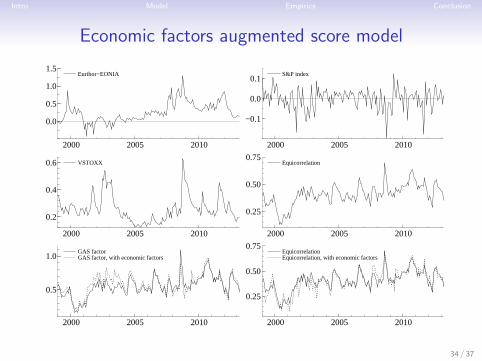
Intro Model Empirics Conclusion
Economic factors augmented score model
Euribor−EONIA
2000 2005 2010
0.0
0.5
1.0
1.5Euribor−EONIA S&P index
2000 2005 2010
−0.1
0.0
0.1S&P index
VSTOXX
2000 2005 2010
0.2
0.4
0.6 VSTOXX Equicorrelation
2000 2005 2010
0.25
0.50
0.75Equicorrelation
GAS factor GAS factor, with economic factors
2000 2005 2010
0.5
1.0GAS factor GAS factor, with economic factors
Equicorrelation Equicorrelation, with economic factors
2000 2005 2010
0.25
0.50
0.75Equicorrelation Equicorrelation, with economic factors
34 / 37
Intro Model Empirics Conclusion
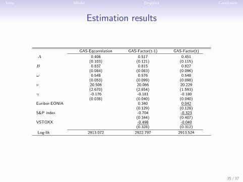
Estimation results
GAS-Eqcorrelation GAS-Factor(t-1) GAS-Factor(t)
A 0.406 0.517 0.451(0.103) (0.121) (0.115)
B 0.837 0.815 0.827(0.084) (0.083) (0.096)
ω 0.548 0.576 0.548(0.053) (0.099) (0.098)
ν 20.506 20.066 20.229(2.670) (2.654) (1.593)
γ -0.176 -0.181 -0.180(0.038) (0.040) (0.040)
Euribor-EONIA 0.340 0.042(0.129) (0.128)
S&P index -0.704 -0.323(0.344) (0.407)
VSTOXX -0.498 -0.040(0.328) (0.312)
Log-lik 2913.072 2922.797 2913.524
35 / 37

Intro Model Empirics Conclusion
Conclusion
How to obtain estimates of financial sector joint tail risk, and tail risk
conditional on a default, if the cross section is very large?
A: GHST-GAS-DECO, a non-Gaussian high-dimensional framework.
Equicorrelation handles large cross sections; works with unbalanced data.
cLLN permits to compute risk measures quickly, without simulation.
Application to euro area financial firms from 1999M1 to 2013M3.
36 / 37

This project is funded by the European Union
under the 7th Framework Programme
(FP7-SSH/2007-2013) Grant Agreement n°320270
www.syrtoproject.eu