American Economic Review 2016, 106(6): 1476–1494 http://dx.doi.org/10.1257/aer.20150208

1476

Measuring Discounting without Measuring Utility†

By Arthur E. Attema, Han Bleichrodt, Yu Gao, Zhenxing Huang, and Peter P. Wakker*

We introduce a new method to measure the temporal discounting of money. Unlike preceding methods, our method requires neither knowledge nor measurement of utility. It is easier to implement, clearer to subjects, and requires fewer measurements than existing methods. (JEL C91, D11, D12, D91)

Discounted utility is the most widely used model to analyze intertemporal deci-sions. It evaluates future outcomes by their utility weighted by a discount factor. Measuring discount factors is difficult because they interact with utility. Most mea-surements simply assume that utility is linear,1 which is unsatisfactory for many economic applications. Frederick, Loewenstein, and O’Donoghue (2002, p. 382), therefore, suggested measuring utility through risky choices while assuming expected utility, as in Chapman (1996), and then to use these utilities to measure discount factors. In the health domain, this method had been used before for flow (continuous) variables (Stiggelbout et al. 1994). In economics, Andersen et al. (2008) and Takeuchi (2011) used this method for discrete outcomes.

The aforementioned method has two limitations. First, expected utility is often violated (Starmer 2000), which distorts utility measurements. Second, the trans-fer of risky cardinal utility to riskless intertemporal choice is controversial (Luce and Raiffa 1957, Fallacy 3; Camerer 1995; Moscati 2013). Andreoni and Sprenger (2012b) and Abdellaoui et al. (2013) provided empirical evidence against such a transfer. When introducing discounted utility, Samuelson (1937, last paragraph) immediately warned that cardinal intertemporal utility may differ from other kinds of cardinal utility. To avoid these two difficulties, some studies elicited both utility and discounting from intertemporal choices (Abdellaoui, Attema, and Bleichrodt 2010; Andreoni and Sprenger 2012a,b; Abdellaoui, Bleichrodt, and l’Haridon 2013;

1 See Warner and Pleeter (2001); Frederick, Loewenstein, and O’Donoghue (2002, p. 381); Tanaka, Camerer, and Nguyen (2010); and Sutter et al. (2013).

* Attema: Institute of Health and Policy Management (iBMG), Erasmus University, PO Box 1738, 3000 DR Rotterdam, the Netherlands (e-mail: attema@bmg.eur.nl); Bleichrodt: Erasmus School of Economics, Erasmus University Rotterdam, PO Box 1738, 3000 DR Rotterdam, the Netherlands (e-mail: bleichrodt@ese.eur.nl); Gao: Department of Management, Economics and Industrial Engineering (DIG), Polytechnic University of Milan, Via Lambruschini 4/b, 20156, Milan, Italy (e-mail: yu.gao@polimi.it); Huang: School of Economics, Shanghai University of Finance and Economics, 111 Wuchuan Road, 200433, Shanghai, China (e-mail: ybhzxadam@gmail.com); Wakker: Erasmus School of Economics, Erasmus University Rotterdam, PO Box 1738, 3000 DR Rotterdam, the Netherlands (e-mail: wakker@ese.eur.nl). The authors declare that they have no relevant or material financial interests that relate to the research described in this paper.

† Go to http://dx.doi.org/10.1257/aer.20150208 to visit the article page for additional materials and author disclosure statement(s).

1477ATTEMA ET AL.: MEASURING DISCOUNTING WITHOUT MEASURING UTILITYVOL. 106 NO. 6

Epper and Fehr-Duda 2015). Such elicitations are complex and susceptible to col-linearities between utility and discounting.

This paper presents a tractable method to measure discounting that requires no knowledge of utility. We adapt a recently introduced method for flow variables in health (Attema, Bleichrodt, and Wakker 2012) to discrete monetary outcomes in economics. Flow variables, such as quality of life, are continuous in time and are consumed per time unit. Whereas theoretical economic studies sometimes take money as a flow variable, experimental studies of discounting invariably take it as discrete, received at discrete time points, and we will do so here. Because our method directly measures discounting, and utility plays no role, we call it the direct method (DM).

The basic idea of the DM is as follows. Assume that a decision maker is indiffer-ent between: (i) an extra payment of $10 per week during weeks 1–30; and (ii) the same extra payment during weeks 31–65. Then the total discount weight of weeks 1–30 is equal to that of weeks 31–65. We can derive the entire discount function from such equalities. Knowledge of utility is not required because it drops from the equations. Even though this method is elementary, it has not been known before.

The DM is easy to implement and subjects can easily understand it. In an exper-iment, we compare it with a traditional, utility-based method (UM). In our com-parison, we use the implementation of the UM by Epper, Fehr-Duda, and Bruhin (2011)—henceforth, EFB—which is based on prospect theory, currently the most accurate descriptive theory of risky choice. We show that the DM needs fewer ques-tions than the UM but gives similar results.

I. Theory

We assume a preference relation ≽ over discrete outcome streams ( x 1 , … , x T ) , yielding outcome (money amount) x j at time t j , for each j ≤ T . For ease of presen-tation, we consider the stimuli used in our experiment, where T = 52 and the unit of time is one week. Thus, ( x 1 , … , x 52 ) yields x j at the end of week j , for each j . Discounted utility holds if preferences maximize the discounted utility of outcome stream x ,

(1) ∑ j=1

52

d j U( x j ) .

Here, U is the subjective utility function, which is strictly increasing and sat-isfies U(0) = 0 , and 0 < d j is the subjective discount factor of week j . For E ⊂ {1, … , 52} , α E β denotes the outcome stream that gives outcome α at all time points in E and outcome β at all other time points. C(E) denotes the cumulative sum ∑ j∈E

d j and reflects the total time weight of E . C(k) denotes C({1, … , k}) . C is

called the cumulative (discount) weight. The proof of the following result clarifies why we do not require utility: it drops from the equations.

OBSERVATION 1: Assume discounted utility, and α > β . Then

(2) α A β ≻ α B β ⇔ ∑ j∈A d j > ∑ j∈B

d j (i.e., C(A) > C(B)) ;

1478 THE AMERICAN ECONOMIC REVIEW JUNE 2016

(3) α A β ∼ α B β ⇔ ∑ j∈A d j = ∑ j∈B

d j (i.e., C(A) = C(B)) ;

(4) α A β ≺ α B β ⇔ ∑ j∈A d j < ∑ j∈B

d j (i.e., C(A) < C(B)) .

PROOF. The preference and two inequalities in equation (2) are each equivalent to

C(A)(U(α) − U(β)) + C({1, … , 52})U(β) > C(B)(U(α) − U(β))

+ C({1, … , 52})U(β) .

The other results follow from similar derivations. ∎

Using Observation 1, we can derive equalities of sums of d j s, which, in turn, define the function C on {1, … , 52} and all the d j s. This procedure does not require any knowledge of utility and is therefore called the direct method (DM).

In the mathematical analysis, we also consider a continuous extension of C , defined on all of (0, 52] , and also called the cumulative (discount) weight. At the time points 1, … , 52 it agrees with C defined above. In the continuous extension, any payoff x j is a salary received during week j . Receiving a salary of x j per week during week j amounts to receiving x j at time j . We equate j with ( j − 1, j ] here. Salary can also be received during part of a week. In the continuous extension, C(t)U(α) is the subjective value of receiving α during period (0, t] , where C(t) = C(0, t] and t may be a noninteger, 0 ≤ t ≤ T . Then C(t, 52] = C(0, 52] − C(0, t] also for nonintegers t . In all the empirical estimations reported later, we extend C from integers to nonintegers using linear interpolations. Given the small time interval of a week, a piecewise linear approximation is satisfactory. The following remark shows that the d j s serve as discretized approximations of the derivative of C .

REMARK 1: d( j) = C( j) − C( j − 1) is the average of the derivative C′ over the interval ( j − 1, j ] . Thus, d j is approximately C′(t) at t = j .

II. Measuring Discounting Using the Direct Method

We now explain how C can be measured up to any degree of precision using the DM. Of course, C(0) = 0 . We normalize C(52) = d 1 + ⋯ + d 52 = 1 . We write c p = C −1 ( p) . Then c 0 = 0 and c 1 = 52 . We take any α > 0 and measure c 1 _ 2 such that α (0, c 1 _ 2 ] 0 ∼ α ( c 1 _ 2 , 52] 0 . By Observation 1, C ( (0, c 1 _ 2 ] ) = C ( ( c 1 _ 2 , 52] )

= 1 _ 2 . Once we know c 1 _ 2 , we can measure c 1 _ 4 and c 3 _ 4 by eliciting indifferences

α (0, c 1 _ 4 ] 0 ∼ α ( c 1 _ 4 , c 1 _ 2 ] 0 and α ( c 1 _ 2 , c 3 _ 4 ] 0 ∼ α ( c 3 _ 4 , 52] 0 . It follows that C ( c 1 _ 4 ) = 1 _ 4 and

C ( c 3 _ 4 ) = 3 _ 4 . In general, we measure subjective midpoints s of time intervals (q, t] by eliciting indifferences α (q, s] β ∼ α (s, t] β (α > β) . By doing this repeatedly, we can measure the cumulative function C to any desired degree of precision. We can then derive the discount factors from C .

1479ATTEMA ET AL.: MEASURING DISCOUNTING WITHOUT MEASURING UTILITYVOL. 106 NO. 6

The DM assumes discounted utility. Its most critical property is separability: a preference ( x 1 , … , x 52 ) ≽ ( y 1 , … , y 52 ) with a common outcome x i = y i = c is not affected if this common outcome is replaced by another common outcome x i = y i = c′ . By repeated application, preference then is independent of any num-ber of common outcomes.

The next proposition shows that the DM permits a simple test of separability, which we implemented in our experiment. The proposition holds for any out-come α > 0 and, more generally, for any pair of outcomes α > β with β instead of 0. The proof is in the Appendix.

PROPOSITION 1: Under weak ordering and separability, we must have

(i) α ( c 1 _ 4 , c 1 _ 2 ] 0 ∼ α ( c 1 _ 2 , c 3 _ 4 ] 0 ;

(ii) α (0, c 1 _ 4 ] 0 ∼ α ( c 3 _ 4 , 52] 0 .

III. The Traditional Utility-Based Method

Our experiment compares the DM with a traditional utility(-based ) method (UM), replicating the implementation by EFB. We first measured prospect theory’s utility function from elicited certainty equivalents of 20 risky options. Next, we measured the money amount λ such that

(5) 9 0 3 0 ∼ λ j 0 ,

where λ j 0 stands for receiving λ at time (week) j and 0 at all other times. Unlike the DM, the UM only involves one-time payments. We chose 9 0 3 0 (and avoided time 0 ) to have stimuli similar to those of the DM. Using the measured utility function U and equation (1) (discounted utility), we derive from equation (5),

(6) d j

u __

d 3 u =

U(90) ______ U(λ) .

Here d j u is the discrete utility based discount factor of week j . We usually normal-

ized d 3 u = 1 .

IV. Experiment

Subjects.—We recruited 104 students (61 percent male; median age 21), mostly economics or finance bachelors, from Erasmus University Rotterdam. The exper-iment was run at the EconLab of Erasmus School of Economics. The data were collected in five sessions. Seven subjects gave erratic answers2 and their data were excluded from the analyses.

2 Debriefings revealed that at least two of these subjects ignored all future payoffs because they had no bank account.

1480 THE AMERICAN ECONOMIC REVIEW JUNE 2016

Incentives.—Each subject was paid a €5 participation fee immediately after the experiment. In addition, we randomly selected (by bingo machine) one subject in each session and then one of his choices to be played out for real. The selections were made in public. We transferred the amount won to the subject’s bank account at the dates specified in the outcome streams. In the DM, subjects made choices between streams of money. Consequently, if one of the DM questions was played out for real, we made bank transfers during several weeks. The five subjects who played for real earned €290 on average. Over the whole group, the average payment per subject was €18.70.

Procedure.—The experiment was computerized. Subjects sat in cubicles to avoid interactions. They could ask questions at any time during the experiment. The exper-iment took 45 minutes on average.

The first part of the experiment consisted of the DM questions, and the second and third part consisted of the UM questions. Subjects could only start each part after they had correctly answered two comprehension questions. Training questions familiarized subjects with the stimuli.

Stimuli: Part 1.—Part 1 consisted of five questions to measure discounting using the DM and two questions to test separability. To measure discounting, we elic-ited c 1 _ 2 , c 1 _ 4 , c 3 _ 4 , c 1 _ 8 , and c 7 _ 8 from the following indifferences:

(7) α (0, c 1 _ 2 ] 0 ∼ α ( c 1 _ 2 , 52] 0, α (0, c 1 _ 4 ] 0 ∼ α ( c 1 _ 4 , c 1 _ 2 ] 0, α ( c 1 _ 2 , c 3 _ 4 ] 0 ∼ α ( c 3 _ 4 , 52] 0,

α (0, c 1 _ 8 ] 0 ∼ α ( c 1 _ 8 , c 1 _ 4 ] 0, and α ( c 3 _ 4 , c 7 _ 8 ] 0 ∼ α ( c 7 _ 8 , 52] 0 .

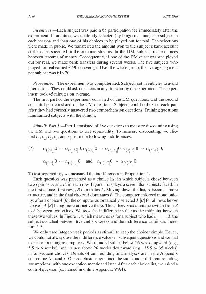
To test separability, we measured the indifferences in Proposition 1.Each question was presented as a choice list in which subjects chose between

two options, A and B , in each row. Figure 1 displays a screen that subjects faced. In the first choice (first row), B dominates A . Moving down the list, A becomes more attractive, and in the final choice A dominates B . The computer enforced monotonic-ity: after a choice A [B] , the computer automatically selected A [B] for all rows below [above], A [B] being more attractive there. Thus, there was a unique switch from B to A between two values. We took the indifference value as the midpoint between these two values. In Figure 1, which measures c 1 _ 8 for a subject who had c 1 _ 4 = 13 , the subject switched between five and six weeks and the indifference value was there-fore 5.5.

We only used integer-week periods as stimuli to keep the choices simple. Hence, we could not always use the indifference values in subsequent questions and we had to make rounding assumptions. We rounded values below 26 weeks upward (e.g., 5.5 to 6 weeks), and values above 26 weeks downward (e.g., 35.5 to 35 weeks) in subsequent choices. Details of our rounding and analyses are in the Appendix and online Appendix. Our conclusions remained the same under different rounding assumptions, with one exception mentioned later. After each choice list, we asked a control question (explained in online Appendix WA4).

1481ATTEMA ET AL.: MEASURING DISCOUNTING WITHOUT MEASURING UTILITYVOL. 106 NO. 6

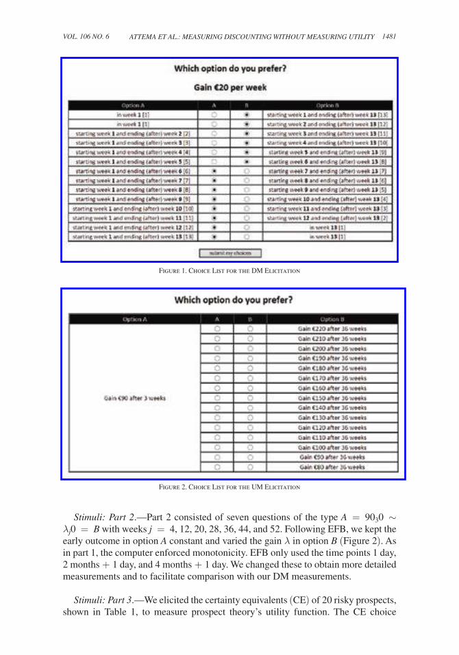
Stimuli: Part 2.—Part 2 consisted of seven questions of the type A = 9 0 3 0 ∼ λ j 0 = B with weeks j = 4, 12, 20, 28, 36, 44, and 52. Following EFB, we kept the early outcome in option A constant and varied the gain λ in option B (Figure 2). As in part 1, the computer enforced monotonicity. EFB only used the time points 1 day, 2 months + 1 day, and 4 months + 1 day. We changed these to obtain more detailed measurements and to facilitate comparison with our DM measurements.

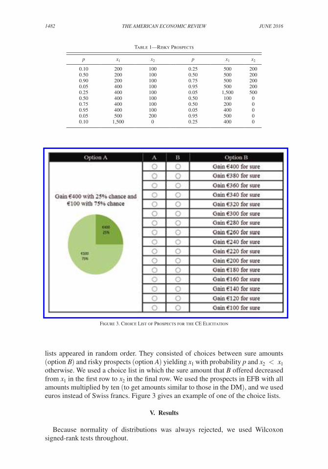
Stimuli: Part 3.—We elicited the certainty equivalents (CE) of 20 risky prospects, shown in Table 1, to measure prospect theory’s utility function. The CE choice

Figure 1. Choice List for the DM Elicitation

Figure 2. Choice List for the UM Elicitation

1482 THE AMERICAN ECONOMIC REVIEW JUNE 2016

lists appeared in random order. They consisted of choices between sure amounts (option B ) and risky prospects (option A ) yielding x 1 with probability p and x 2 < x 1 otherwise. We used a choice list in which the sure amount that B offered decreased from x 1 in the first row to x 2 in the final row. We used the prospects in EFB with all amounts multiplied by ten (to get amounts similar to those in the DM), and we used euros instead of Swiss francs. Figure 3 gives an example of one of the choice lists.

V. Results

Because normality of distributions was always rejected, we used Wilcoxon signed-rank tests throughout.

Table 1—Risky Prospects

p x 1 x 2 p x 1 x 2

0.10 200 100 0.25 500 2000.50 200 100 0.50 500 2000.90 200 100 0.75 500 2000.05 400 100 0.95 500 2000.25 400 100 0.05 1,500 5000.50 400 100 0.50 100 00.75 400 100 0.50 200 00.95 400 100 0.05 400 00.05 500 200 0.95 500 00.10 1,500 0 0.25 400 0

Figure 3. Choice List of Prospects for the CE Elicitation

1483ATTEMA ET AL.: MEASURING DISCOUNTING WITHOUT MEASURING UTILITYVOL. 106 NO. 6

A. Results for the DM

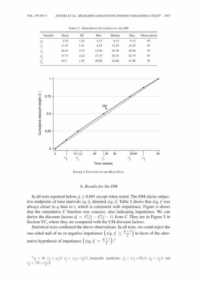
In all tests reported below, p ≤ 0.001 except when noted. The DM elicits subjec-tive midpoints of time intervals (q, t] , denoted s(q, t] . Table 2 shows that s(q, t] was always closer to q than to t , which is consistent with impatience. Figure 4 shows that the cumulative C function was concave, also indicating impatience. We can derive the discount factors d j = C( j) − C( j − 1) from C . They are in Figure 5 in Section VC, where they are compared with the UM discount factors.

Statistical tests confirmed the above observations. In all tests, we could reject the

one-sided null of no or negative impatience (s(q, t] ≥ q + t

____ 2 ) in favor of the alter-

native hypothesis of impatience (s(q, t] < q + t

____ 2 ) .3

3 c 1 __ 2

< 26 , c 1 __ 4

< c 1 __ 2

/2 , c 1 __ 2

< ( c 1 __ 4

+ c 3 __ 4

)/2 (marginally significant), c 3 __ 4 < ( c 1 __

2 + 52)/2 , c 1 __

8 < c 1 __

4 /2 , and

c 7 __ 8

< (52 + c 3 __ 4

)/2 .

0

0.25

0.5

0.75

1

Cum

ulat

ive

disc

ount

wei

ght (

C)

0 5210 20 30 4026

Time (weeks)

13 39

DM

c 18

c14

c12

c34

c 78

Table 2—Descriptive Statistics of the DM

Variable Mean SD Min Median Max Observations

c 1 _ 8 5.55 1.25 2.13 6.13 9.13 97

c 1 _ 4 11.47 1.91 4.25 12.25 15.25 97

c 1 _ 2 24.47 2.72 14.50 25.50 29.50 97

c 3 _ 4 37.77 2.22 27.75 38.75 42.75 97

c 7 _ 8 44.5 1.45 39.88 44.88 47.88 97

Figure 4. Function of the Mean Data

1484 THE AMERICAN ECONOMIC REVIEW JUNE 2016

Decreasing impatience, found in many studies, implies that c 1 _ 2 /2 − c 1 _ 4 > ( c 1 _ 2 + 52) /2 − c 3 _ 4 and c 1 _ 4 /2 − c 1 _ 8 > ( c 3 _ 4 + 52) /2 − c 7 _ 8 . The evidence on decreas-ing impatience was mixed and depended on the rounding assumption used (see the online Appendix). Under one rounding assumption, we found decreasing impa-tience in the comparison between (0, c 1 _ 2 ] and ( c 1 _ 2 , 52] and increasing impatience in

the comparison between (0, c 1 _ 4 ] and ( c 3 _ 4 , 52] . Under another rounding assumption,4 the null of constant impatience could not be rejected. For all other tests in this paper, the rounding assumptions were immaterial.

To test separability condition (i) in Proposition 1, we directly measured the sub-jective midpoint s 1 _ 2 of ( c 1 _ 4 , c 3 _ 4 ] . That is, α ( c 1 _ 4 , s 1 _ 2 ] 0 ∼ α ( s 1 _ 2 , c 3 _ 4 ] 0 . By condition (i), s 1 _ 2

should equal c 1 _ 2 . To test separability condition (ii) in Proposition 1, we directly mea-sured the value s 3 _ 4 such that α (0, c 1 _ 4 ] 0 ∼ α ( s 3 _ 4 , 52] 0 . This second measurement is of a

different nature than the questions asked in the rest of the experiment, because now a lower point of an interval is determined rather than a midpoint. By condition (ii), s 3 _ 4 should equal c 3 _ 4 .

Separability was rejected in the first test ( p < 0.01 two-sided), but not in the second. Even in the first test, we found few violations of separability at the individ-ual level. Separability was satisfied exactly for 54 out of 97 subjects. Moreover, s 1 _ 2 and c 1 _ 2 differed by 1 at most for 80 subjects. In the second test, separability could not hold exactly due to rounding, but 55 subjects had the minimal difference of 0.5, and 76 subjects had the difference 1.5 or less.

B. Results for the UM

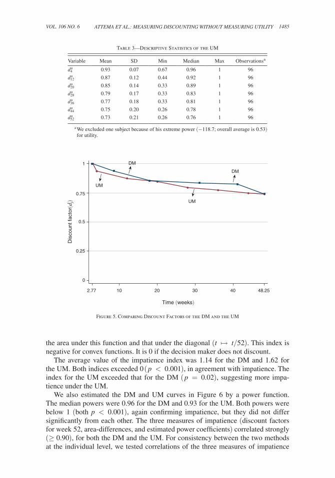
Table 3 summarizes the descriptive statistics of the discount factors d j u under the

normalization d 3 u = 1 , the discount factor of the shortest delay in the UM. Comparing

pairs of consecutive discount factors confirmed impatience (always p < 0.001 ). We derived the cumulative function C u ( j) = ∑ i=1

j d i

u from the discount factors. For easy comparison with the DM, we renormalized C u (52) = 1 for C u .

C. Comparing Discounting and Impatience under the DM and the UM

Figure 5 shows the discount factors of the DM and the UM. For easy comparison, we normalized both to 1 at week three here. Both discount factors were decreasing, confirming impatience. The DM discount factors slightly exceeded the UM discount factors, but not significantly (tests provided later). According to both methods, the annual discount rate was 35 percent, assuming continuous compounding e −r t with t in years.

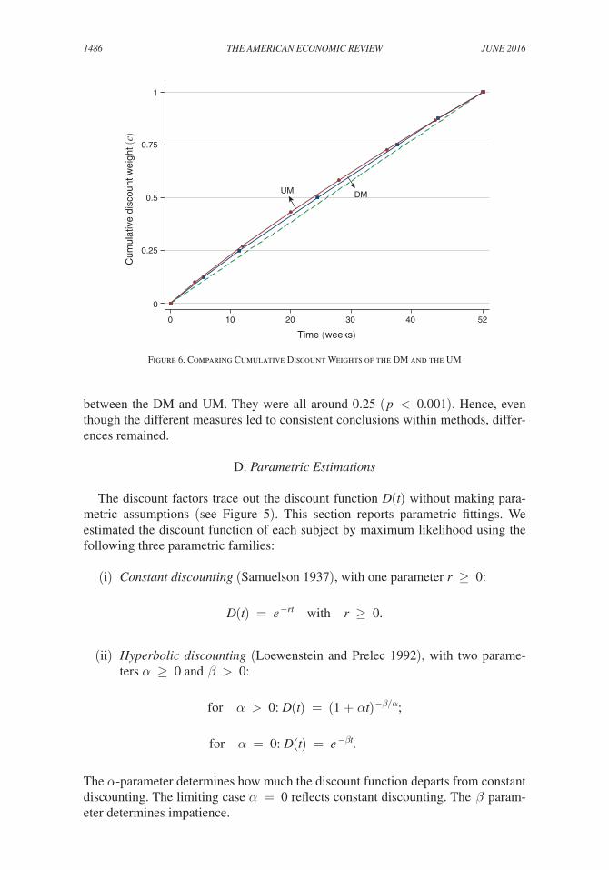
Figure 6 shows the cumulative functions of the DM and the UM, using linear interpolation to obtain general values d j

u from the seven measured d j u s. We measured

impatience (= concavity) for each cumulative function by the difference between

4 A large middle group ( n = 37 ) gave answers as close as possible to constant discounting. The first rounding takes them as slightly impatient. It can also be argued that the null of constant discounting should be accepted for them (our second rounding).

1485ATTEMA ET AL.: MEASURING DISCOUNTING WITHOUT MEASURING UTILITYVOL. 106 NO. 6

the area under this function and that under the diagonal ( t ↦ t/52 ). This index is negative for convex functions. It is 0 if the decision maker does not discount.

The average value of the impatience index was 1.14 for the DM and 1.62 for the UM. Both indices exceeded 0 ( p < 0.001 ), in agreement with impatience. The index for the UM exceeded that for the DM ( p = 0.02 ), suggesting more impa-tience under the UM.

We also estimated the DM and UM curves in Figure 6 by a power function. The median powers were 0.96 for the DM and 0.93 for the UM. Both powers were below 1 (both p < 0.001 ), again confirming impatience, but they did not differ significantly from each other. The three measures of impatience (discount factors for week 52, area-differences, and estimated power coefficients) correlated strongly (≥ 0.90), for both the DM and the UM. For consistency between the two methods at the individual level, we tested correlations of the three measures of impatience

0

0.25

0.5

0.75

1

Dis

coun

t fac

tor(

d j)

2.77 48.2510 20 30 40

Time (weeks)

UM

UM

DM

DM

Table 3—Descriptive Statistics of the UM

Variable Mean SD Min Median Max Observationsa

d 4 u 0.93 0.07 0.67 0.96 1 96

d 12 u 0.87 0.12 0.44 0.92 1 96

d 20 u 0.85 0.14 0.33 0.89 1 96

d 28 u 0.79 0.17 0.33 0.83 1 96

d 36 u 0.77 0.18 0.33 0.81 1 96

d 44 u 0.75 0.20 0.26 0.78 1 96

d 52 u 0.73 0.21 0.26 0.76 1 96

a We excluded one subject because of his extreme power (−118.7; overall average is 0.53) for utility.

Figure 5. Comparing Discount Factors of the DM and the UM

1486 THE AMERICAN ECONOMIC REVIEW JUNE 2016

between the DM and UM. They were all around 0.25 ( p < 0.001). Hence, even though the different measures led to consistent conclusions within methods, differ-ences remained.

D. Parametric Estimations

The discount factors trace out the discount function D(t) without making para-metric assumptions (see Figure 5). This section reports parametric fittings. We estimated the discount function of each subject by maximum likelihood using the following three parametric families:

(i) Constant discounting (Samuelson 1937), with one parameter r ≥ 0 :

D(t) = e −rt with r ≥ 0 .

(ii) Hyperbolic discounting (Loewenstein and Prelec 1992), with two parame-ters α ≥ 0 and β > 0 :

for α > 0: D(t) = (1 + αt ) −β/α ;

for α = 0: D(t) = e −βt .

The α -parameter determines how much the discount function departs from constant discounting. The limiting case α = 0 reflects constant discounting. The β param-eter determines impatience.

0

0.25

0.5

0.75

1

Cum

ulat

ive

disc

ount

wei

ght (

c)

0 5210 20 30 40

Time (weeks)

UM DM

Figure 6. Comparing Cumulative Discount Weights of the DM and the UM

1487ATTEMA ET AL.: MEASURING DISCOUNTING WITHOUT MEASURING UTILITYVOL. 106 NO. 6

(iii) Unit-invariance discounting,5 with two parameters r > 0 and d :

for d > 1 , D(t) = exp (r t 1−d ) (only if t = 0 is not considered);

for d = 1 , D(t) = t −r (only if t = 0 is not considered);

for d < 1 , D(t) = exp (−r t 1−d ) .

The r -parameter determines impatience and the d -parameter determines departure from constant discounting, interpreted as sensitivity to time by Ebert and Prelec (2007). The common empirical finding is d ≤ 1 , reflecting insensitivity.

Hyperbolic discounting can only account for decreasing impatience. However, empirical studies have observed that a substantial proportion of subjects are not decreasingly, but increasingly impatient (references in Section VE). Unit-invariance discounting can account for both decreasing and increasing impatience. We can use the entire unit-invariance family because our domain does not contain t = 0 (explained in the discussion section). The exclusion of t = 0 also implies that the popular quasihyperbolic family coincides with constant discounting for our stimuli.

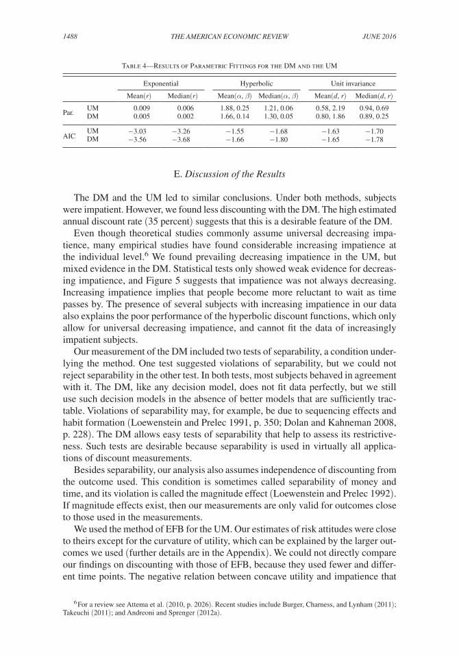
Table 4 shows the estimated parameters. The exponential discounting parameters differed between the UM and the DM ( p < 0.001 ), reflecting more discounting for the UM. The parameters of hyperbolic discounting and unit-invariance discounting did not differ significantly ( p > 0.2 ).

The final two rows of Table 4 show the goodness-of-fit of the three discount fami-lies by the Akaike information criterion (AIC). More-negative values indicate better fit. The DM with exponential discounting fitted better than the UM with exponential discounting ( p < 0.001 ), and gave the best fit overall. The DM also seemed to fit better for hyperbolic discounting and unit invariance, but these differences were not significant. Of the three parametric families, exponential discounting fitted best for both the DM and the UM (both p < 0.001 ). For the UM, hyperbolic discounting gave the worst fit ( p < 0.001 ). For the DM we found no significant difference between unit invariance and hyperbolic discounting ( p = 0.22 ). In the absence of the immediacy effect, exponential discounting performed well, which also supports quasihyperbolic discounting. The online Appendix gives further details.

We, finally, investigated the relation between impatience (concavity of C and C u ) and risk attitudes, controlling for demographic variables (age, gender, and foreign versus domestic—Dutch). Impatience under the UM was negatively related with concavity of utility, which is not surprising because the UM measurements were based on utility. Under the DM, impatience was not related with utility, suggesting that these are independent components. Impatience under the UM was also nega-tively related with risk aversion in the form of pessimism of probability weighting, in contrast to impatience under the DM. Age was positively related with UM impa-tience. Other relations were not significant. Details are in the online Appendix.

5 Read (2001, equation 16) first suggested this family. Ebert and Prelec (2007) called it constant sensitivity, and Bleichrodt, Rohde, and Wakker (2009) called it constant relative decreasing impatience. Bleichrodt et al. (2013) proposed the term unit invariance.

1488 THE AMERICAN ECONOMIC REVIEW JUNE 2016

E. Discussion of the Results

The DM and the UM led to similar conclusions. Under both methods, subjects were impatient. However, we found less discounting with the DM. The high estimated annual discount rate (35 percent) suggests that this is a desirable feature of the DM.

Even though theoretical studies commonly assume universal decreasing impa-tience, many empirical studies have found considerable increasing impatience at the individual level.6 We found prevailing decreasing impatience in the UM, but mixed evidence in the DM. Statistical tests only showed weak evidence for decreas-ing impatience, and Figure 5 suggests that impatience was not always decreasing. Increasing impatience implies that people become more reluctant to wait as time passes by. The presence of several subjects with increasing impatience in our data also explains the poor performance of the hyperbolic discount functions, which only allow for universal decreasing impatience, and cannot fit the data of increasingly impatient subjects.

Our measurement of the DM included two tests of separability, a condition under-lying the method. One test suggested violations of separability, but we could not reject separability in the other test. In both tests, most subjects behaved in agreement with it. The DM, like any decision model, does not fit data perfectly, but we still use such decision models in the absence of better models that are sufficiently trac-table. Violations of separability may, for example, be due to sequencing effects and habit formation (Loewenstein and Prelec 1991, p. 350; Dolan and Kahneman 2008, p. 228). The DM allows easy tests of separability that help to assess its restrictive-ness. Such tests are desirable because separability is used in virtually all applica-tions of discount measurements.

Besides separability, our analysis also assumes independence of discounting from the outcome used. This condition is sometimes called separability of money and time, and its violation is called the magnitude effect (Loewenstein and Prelec 1992). If magnitude effects exist, then our measurements are only valid for outcomes close to those used in the measurements.

We used the method of EFB for the UM. Our estimates of risk attitudes were close to theirs except for the curvature of utility, which can be explained by the larger out-comes we used (further details are in the Appendix). We could not directly compare our findings on discounting with those of EFB, because they used fewer and differ-ent time points. The negative relation between concave utility and impatience that

6 For a review see Attema et al. (2010, p. 2026). Recent studies include Burger, Charness, and Lynham (2011); Takeuchi (2011); and Andreoni and Sprenger (2012a).

Table 4—Results of Parametric Fittings for the DM and the UM

Exponential Hyperbolic Unit invariance

Mean( r ) Median( r ) Mean( α, β ) Median( α, β ) Mean( d, r ) Median( d, r )

Par.UM 0.009 0.006 1.88, 0.25 1.21, 0.06 0.58, 2.19 0.94, 0.69DM 0.005 0.002 1.66, 0.14 1.30, 0.05 0.80, 1.86 0.89, 0.25

AICUM −3.03 −3.26 −1.55 −1.68 −1.63 −1.70DM −3.56 −3.68 −1.66 −1.80 −1.65 −1.78

1489ATTEMA ET AL.: MEASURING DISCOUNTING WITHOUT MEASURING UTILITYVOL. 106 NO. 6

we found for the UM is not surprising because utility plays a central role in the UM. Concave utility increases the ratio in equation (6) and thus decreases impatience. The negative relation between impatience and probability weighting suggests that this component of risk attitude also affects the UM measurements. Our findings suggest that there is collinearity between utility/risk attitude and discounting in the UM, but not in the DM.

Our implementation of the DM is adaptive, with answers to questions influencing the stimuli in later questions. Theoretically, this may offer scope for manipulation: responding untruthfully to some questions may improve later stimuli. However, according to the Bardsley et al. (2010, p. 265) classification, this possibility is only theoretical and is no cause for concern in our experiment. First, it was vir-tually impossible for subjects to realize that questions were adaptive because of the roundings used. Second, we expect that even readers who like us, are aware of the adaptive nature and even of the stimuli of our experiment beforehand, are not likely to see how the loss of wrongly answering one question could be compensated by advantages in follow-up questions. This would be impossible for our subjects. Online Appendix WE gives details. For these two reasons, manipulation is only a theoretical concern for our experiment.

The DM can be implemented nonadaptively. For example, we can select a num-ber of outcome streams α A j β and time points s j beforehand, and measure the time points t j such that α A j β ∼ α ( s j , t j ] β for all j . Observation 1 still gives equalities C ( A j ) = C ( s j , t j ] . We can use these in parametric fittings of C or in tests of prop-erties such as decreasing impatience, without requiring knowledge about U . A drawback of this nonadaptive procedure is that we then cannot readily draw a con-nected C -curve as in Figures 4 and 6, where we needed no parametric assumption (other than linear interpolation).

The DM always had a better fit than the UM, and exponential discounting always fitted best, with unit invariance second best. Exponential discounting could perform well because we did not include the present t = 0 in our stimuli, where most vio-lations are found due to the immediacy effect (Attema 2012). Although this effect is important and deserves further study, we decided to focus our first implementa-tion of the DM on a better understood empirical domain, which we could compare directly with EFB. In this regard, we follow many other studies in the literature that use front-end delays.

The DM can readily investigate the immediacy effect and discrete outcomes at t = 0 . The latter are then interpreted as salaries paid at the beginning, instead of at the end of periods (weeks in our case). Given that the relations that we made with flow variables only served as intermediate tools in our mathematical analysis, and played no role in the stimuli or results, we can use the interpretation mentioned. Quasihyperbolic discounting then implies a high weight for the first week of salary (now mathematically representing the present rather than the time point one week ahead), and moderate weights for the other weeks.

VI. General Discussion

Attema et al. (2010) measured discounting up to a power without the need to know utility, but needed separate measurements to identify the power. Unlike the

1490 THE AMERICAN ECONOMIC REVIEW JUNE 2016

DM but like the UM, their measurements did not need time separability, but they could not test it either. In a mathematical sense, our method is similar to the mea-surement of subjective probability based on equal likelihood assessments, where utility also drops from the equations and separability (now over events) is assumed (Baillon 2008).

Subjective midpoints, used by the DM to measure discounting, have a long tradi-tion in psychophysics (bisection; Stevens 1936) and mathematics ( quasi-arithmetic mean; Aczél 1966). Condition (i) in Proposition 1, a necessary condition of a quasi-arithmetic mean, is a special case of autodistributivity (Aczél 1966, equation (6.4.2.3), for t the midpoint of x and y ).

To our best knowledge, all experimental measurements of money discounting have used discrete outcomes. Real-life decisions often involve flow outcomes that are repeated per time unit. Examples are salary payments, pension saving plans, and mortgage debt repayments. In such contexts, the DM is more natural than discrete methods such as the UM. For discrete outcomes, the DM can be an alternative to the UM if the payments are sufficiently frequent and the periods are sufficiently fine, as in our experiment. However, the DM is less useful for decisions in which outcomes occur infrequently, such as for single-outcome decisions.

In the DM, subjects only make trade-offs between periods. In the UM, subjects make trade-offs both between outcomes and between periods, which is more com-plex. Hence, the DM is easier for subjects. Our experiment gave indirect support: we found a positive correlation between utility curvature and discounting for the UM, but not for the DM, showing that outcome trade-offs impact time trade-offs in the UM but not in the DM.

The DM is also easier to use for researchers, because of the elementary nature of Observation 1. In the DM, we only used seven questions. In the UM, we also used seven questions7 to elicit discounting, but we needed additional questions to elicit utility. The DM took much less time.

The DM can be analyzed using parametric econometric fittings (Section VD), as can all existing methods, but, unlike most methods, the DM can also be analyzed in a parameter-free way (Section VA). This reveals the correct discount function with-out a commitment to a parametric family of discount functions. The DM can also be used for interactive prescriptive measurements in consultancy applications (Keeney and Raiffa 1976).

VII. Conclusion

This paper has introduced a new method to measure the discounting of money, the direct method. This method is simpler than existing methods because it does not need information about utility. Consequently, the experimental tasks are easier for subjects, researchers have to ask fewer questions, and the measurements are not dis-torted by biases in utility. An experiment confirms the implementability and validity of the direct method.

7 We used the same numbers of questions to make the methods comparable. In fact, two DM questions tested separability. The DM derived the discount functions from only five measurements.

1491ATTEMA ET AL.: MEASURING DISCOUNTING WITHOUT MEASURING UTILITYVOL. 106 NO. 6

Appendix A: Proofs

PROOF OF PROPOSITION 1: This proof is elementary in not using technical assumptions such as con-

tinuity. The proof only uses the two outcomes used in the preferences, being α and 0 . For deriving the first indifference, we denote outcome streams as quadru-ples ( x 1 , x 2 , x 3 , x 4 ) , with x 1 received in (0, c 1 _ 4 ] , x 2 in ( c 1 _ 4 , c 1 _ 2 ] , x 3 in ( c 1 _ 2 , c 3 _ 4 ] , and x 4 in

( c 3 _ 4 , 52] . We only use the following parts of equation (7): (α, α, 0, 0) ∼ (0, 0, α, α) (1), (α, 0, 0, 0) ∼ (0, α, 0, 0) (2), and (0, 0, α, 0) ∼ (0, 0, 0, α) (3). Assume, for contradiction, that (i) is violated, say (0, α, 0, 0) ≻ (0, 0, α, 0) (4). This, (2), (3), and transitivity, imply (α, 0, 0, 0) ≻ (0, 0, 0, α) (5). By separability, (4) implies (α, α, 0, 0) ≻ (α, 0, α, 0) , and (5) implies (α, 0, α, 0) ≻ (0, 0, α, α) . By transitivity, (α, α, 0, 0) ≻ (0, 0, α, α) , contradicting (1). Reversing all preferences shows that (0, α, 0, 0) ≺ (0, 0, α, 0) implies the contradictory (α, α, 0, 0) ≺ (0, 0, α, α) . The indifference in (i) has been proved. The second indifference fol-lows from the first, (2), (3), and transitivity. ∎

Appendix B: Details of the DM

Preferences α {1, … , j} 0 ≺ α { j+1, … , 52} 0 and α {1, … , j+1} 0 ≻ α { j+2, … , 52} 0 reveal that c 1 _ 2 is in the interval ( j, j + 1) . We then estimate c 1 _ 2 = j + 1 _ 2 . For the DM, we used the following roundings to derive the discount factors from the C function (Figure 5). For each of the six periods considered (bounded by t = 0 , the five c p values that we measured, and t = 52 ), we divided the increase of C over this period by the length of the period to obtain the average week-weight d over this period. We assigned this d value to the midpoint of the period, and we used linear interpolation between these midpoints. We normalized (setting d = 1 ) at the smallest positive time point considered, being c 1 _ 8 /2. Its average (2.75) was approximately 3, leading to about the same normalization as with the UM. Thus, we obtained a d -function over the interval (3, 48.25], with 48.25 the average midpoint of the last interval ( c 7 _ 8 , 52] .

Because we only presented integer-week periods to subjects, and estimates of c p were usually nonintegers, we could not present exact c p values to our sub-jects in our adaptive experiment. For example, to find the subjective midpoint c 1 _ 4

of (0, c 1 _ 2 ] , we rounded c 1 _ 2 and took (assuming it is below 26) the smallest larger

integer, denoted j + 1 here, and then found the subjective midpoint x of (0, j + 1] . To derive c 1 _ 4 from this midpoint x , we corrected for the roundings. Because we had used j + 1 instead of c 1 _ 2 , which on average is an overestimation of c 1 _ 2 by 1 _ 2 , and half of it will propagate into x , we subtracted 1 _ 4 from x to get c 1 _ 4 . In all other estimations of values c p , we similarly used roundings and corrections. Complete details of the roundings and corrections for all c p are in the online Appendix.

1492 THE AMERICAN ECONOMIC REVIEW JUNE 2016

Appendix C: Details of the UM

Following EFB, we adopted power utility (Wakker 2008) and Prelec’s (1998) two-parameter probability weighting:

If η > 0 , then u(x) = x η ;

If η = 0 , then u(x) = ln(x) ;

If η < 0 , then u(x) = − x η ;

w( p) = e −β(−ln( p) ) α .

For convenience, x is generic for outcomes in this Appendix. The average value of the utility parameter η was 0.47 (in EFB, η = 0.87 ), which reflects concavity.8 The difference found can be explained by the higher outcomes we used. The average insensitivity index α was 0.55 (in EFB, α = 0.51 ), indicating departure from linear probability weighting. The average estimates for the pessimism index β was 0.94 (in EFB, β = 0.97 ).

In equation (6) we should have U(0) = 0 , which agrees with prospect theory’s scaling. Following EFB, the estimation of utility is carried out after shifting all out-comes by one unit of money, so as to avoid mathematical complications of logarith-mic or negative-power utility at x = 0 .

We followed EFB in using choice lists to elicit λ in equation (5) (details are in the online Appendix). If the largest value in a choice list was still too small to lead to preference, we assumed preference to switch in the first higher value to follow. We thus use censored data. It gives a smaller bias than dropping these subjects, the most impatient ones, as done by EFB, and it keeps more subjects for other measurements. The DM measurements need no censoring of data because the indifference points are always between extremes of the choice lists.

REFERENCES

Abdellaoui, Mohammed, Arthur E. Attema, and Han Bleichrodt. 2010. “Intertemporal Tradeoffs for Gains and Losses: An Experimental Measurement of Discounted Utility.” Economic Journal 120 (545): 845–66.

Abdellaoui, Mohammed, Han Bleichrodt, and Olivier l’Haridon. 2013. “Sign-Dependence in Inter-temporal Choice.” Journal of Risk and Uncertainty 47 (3): 225–53.

Abdellaoui, Mohammed, Han Bleichrodt, Olivier L’Haridon, and Corina Paraschiv. 2013. “Is There One Unifying Concept of Utility? An Experimental Comparison of Utility under Risk and Utility over Time.” Management Science 59 (9): 2153–69.

Aczél, János. 1966. Lectures on Functional Equations and Their Applications. New York: Academic Press.

Andersen, Steffen, Glenn W. Harrison, Morten I. Lau, and E. Elisabet Rutström. 2008. “Eliciting Risk and Time Preferences.” Econometrica 76 (3): 583–618.

Andreoni, James, and Charles Sprenger. 2012a. “Estimating Time Preference from Convex Budgets.” American Economic Review 102 (7): 3333–56.

8 The average value of the parameters in our analysis is based on 96 subjects (including subjects who have missing values). EFB removed all subjects with missing values.

1493ATTEMA ET AL.: MEASURING DISCOUNTING WITHOUT MEASURING UTILITYVOL. 106 NO. 6

Andreoni, James, and Charles Sprenger. 2012b. “Risk Preferences Are Not Time Preferences.” Amer-ican Economic Review 102 (7): 3357–76.

Attema, Arthur E. 2012. “Developments in Time Preference and Their Implications for Medical Deci-sion Making.” Journal of the Operational Research Society 63 (10): 1388–99.

Attema, Arthur E., Han Bleichrodt, Yu Gao, Zhenxing Huang, and Peter P. Wakker. 2016. “Measur-ing Discounting without Measuring Utility: Dataset.” American Economic Review. http://dx.doi.org/10.1257/aer.20150208.

Attema, Arthur E., Han Bleichrodt, Kirsten I. M. Rohde, and Peter P. Wakker. 2010. “Time-Tradeoff Sequences for Analyzing Discounting and Time Inconsistency.” Management Science 56 (11): 2015–30.

Attema, Arthur E., Han Bleichrodt, and Peter P. Wakker. 2012. “A Direct Method for Measuring Dis-counting and QALYs more Easily and Reliably.” Medical Decision Making 32 (4): 583–93.

Baillon, Aurélien. 2008. “Eliciting Subjective Probabilities through Exchangeable Events: An Advan-tage and a Limitation.” Decision Analysis 5 (2): 76–87.

Bardsley, Nicholas, Robin Cubitt, Graham Loomes, Peter Moffat, Chris Starmer, and Robert Sugden. 2010. Experimental Economics: Rethinking the Rules. Princeton, NJ: Princeton University Press.

Bleichrodt, Han, Amit Kothiyal, Drazen Prelec, and Peter P. Wakker. 2013. “Compound Invariance Implies Prospect Theory for Simple Prospects.” Journal of Mathematical Psychology 57 (3–4): 68–77.

Bleichrodt, Han, Kirsten I. M. Rohde, and Peter P. Wakker. 2009. “Non-Hyperbolic Time Inconsis-tency.” Games and Economic Behavior 66 (1): 27–38.

Burger, Nicholas, Gary Charness, and John Lynham. 2011. “Field and Online Experiments on Self-Control.” Journal of Economic Behavior & Organization 77 (3): 393–404.

Camerer, Colin F. 1995. “Individual Decision Making.” In Handbook of Experimental Economics, edited by John H. Kagel and Alvin E. Roth, 587–703. Princeton, NJ: Princeton University Press.

Chapman, Gretchen B. 1996. “Expectations and Preferences for Sequences of Health and Money.” Organizational Behavior and Human Decision Processes 67 (1): 59–75.

Dolan, Paul, and Daniel Kahneman. 2008. “Interpretations of Utility and Their Implications for the Valuation of Health.” Economic Journal 118 (525): 215–34.

Ebert, Jane E. J., and Drazen Prelec. 2007. “The Fragility of Time: Time-Insensitivity and Valuation of the Near and Far Future.” Management Science 53 (9): 1423–38.

Epper, Thomas, and Helga Fehr-Duda. 2015. “Risk Preferences Are Not Time Preferences: Balancing on a Budget Line: Comment.” American Economic Review 105 (7): 2261–71.

Epper, Thomas, Helga Fehr-Duda, and Adrian Bruhin. 2011. “Viewing the Future through a Warped Lens: Why Uncertainty Generates Hyperbolic Discounting.” Journal of Risk and Uncertainty 43 (3): 163–203.

Frederick, Shane, George Loewenstein, and Ted O’Donoghue. 2002. “Time Discounting and Time Preference: A Critical Review.” Journal of Economic Literature 40 (2): 351–401.

Keeney, Ralph L., and Howard Raiffa. (1976) 1993. Decisions with Multiple Objectives: Preferences and Value Tradeoffs. 2nd ed. Cambridge, UK: Cambridge University Press.

Loewenstein, George F., and Drazen Prelec. 1991. “Negative Time Preference.” American Economic Review 81 (2): 347–52.

Loewenstein, George F., and Drazen Prelec. 1992. “Anomalies in Intertemporal Choice: Evidence and an Interpretation.” Quarterly Journal of Economics 107: 573–97.

Luce, R. Duncan, and Howard Raiffa. 1957. Games and Decisions. New York: Wiley.Moscati, Ivan. 2013. “How Cardinal Utility Entered Economic Analysis, 1909–1944.” European Jour-

nal of the History of Economic Thought 20 (6): 906–39.Prelec, Drazen. 1998. “The Probability Weighting Function.” Econometrica 66 (3): 497–527.Read, Daniel. 2001. “Is Time-Discounting Hyperbolic or Subadditive?” Journal of Risk and Uncer-

tainty 23 (1): 5–32.Samuelson, Paul A. 1937. “A Note on Measurement of Utility.” Review of Economic Studies 4 (2):

155–61.Starmer, Chris. 2000. “Developments in Non-Expected Utility Theory: The Hunt for a Descriptive

Theory of Choice under Risk.” Journal of Economic Literature 38 (2): 332–82.Stevens, Stanley S. 1936. “A Scale for the Measurement of a Psychological Magnitude: Loudness.”

Psychological Review 43 (5): 405–16.Stiggelbout, Anne M., Gwendoline M. Kiebert, Job Kievit, Jan W. H. Leer, Gerrit Stoter, and Hanneke

C. J. M. de Haes. 1994. “Utility Assessment in Cancer Patients: Adjustment of Time Tradeoff Scores for the Utility of Life Years and Comparison with Standard Gamble Scores.” Medical Deci-sion Making 14 (1): 82–90.

1494 THE AMERICAN ECONOMIC REVIEW JUNE 2016

Sutter, Matthias, Martin G. Kocher, Daniela Glätzle-Rüetzler, and Stefan T. Trautmann. 2013. “Impa-tience and Uncertainty: Experimental Decisions Predict Adolescents’ Field Behavior.” American Economic Review 103 (1): 510–31.

Takeuchi, Kan. 2011. “Non-Parametric Test of Time Consistency: Present Bias and Future Bias.” Games and Economic Behavior 71 (2): 456–78.

Tanaka, Tomomi, Colin F. Camerer, and Quang Nguyen. 2010. “Risk and Time Preferences: Linking Experimental and Household Survey Data from Vietnam.” American Economic Review 100 (1): 557–71.

Wakker, Peter P. 2008. “Explaining the Characteristics of the Power (CRRA) Utility Family.” Health Economics 17 (12): 1329–44.

Warner, John T., and Saul Pleeter. 2001. “The Personal Discount Rate: Evidence from Military Down-sizing Programs.” American Economic Review 91 (3): 33–53.