measuring expectations from household surveys: …€¦ · measuring expectations from household...
TRANSCRIPT

MEASURING EXPECTATIONS FROM HOUSEHOLD SURVEYS: NEW RESULTS ON SUBJECTIVE PROBABILITIES OF FUTURE HOUSE PRICES
Olympia Bover
Documentos de Trabajo N.º 1535
2015

MEASURING EXPECTATIONS FROM HOUSEHOLD SURVEYS:
NEW RESULTS ON SUBJECTIVE PROBABILITIES OF FUTURE HOUSE PRICES

Documentos de Trabajo. N.º 1535
2015
(*) This paper was written as a lecture for presentation as the Presidential Address to the Congress of the Spanish Economic Association in Vigo, December 2012. I am grateful to an anonymous referee and the Editor for their helpful comments.
Olympia Bover
BANCO DE ESPAÑA
MEASURING EXPECTATIONS FROM HOUSEHOLD SURVEYS:
NEW RESULTS ON SUBJECTIVE PROBABILITIES OF FUTURE
HOUSE PRICES (*)

The Working Paper Series seeks to disseminate original research in economics and fi nance. All papers have been anonymously refereed. By publishing these papers, the Banco de España aims to contribute to economic analysis and, in particular, to knowledge of the Spanish economy and its international environment.
The opinions and analyses in the Working Paper Series are the responsibility of the authors and, therefore, do not necessarily coincide with those of the Banco de España or the Eurosystem.
The Banco de España disseminates its main reports and most of its publications via the Internet at the following website: http://www.bde.es.
Reproduction for educational and non-commercial purposes is permitted provided that the source is acknowledged.
© BANCO DE ESPAÑA, Madrid, 2015
ISSN: 1579-8666 (on line)

Abstract
I analyse new data on subjective probabilistic expectations on house prices collected in
the Spanish Survey of Household Finances. Households are asked to distribute ten points
among fi ve different scenarios for the change in the price of their homes over the next 12
months. This paper is the fi rst empirical study to document the beliefs of a representative
sample of households about the future value of their homes. It also reviews the methodology
of expectation measurement and recent work on household subjective probabilities. I model
individual subjective probability densities using splines, construct quantiles from those
densities, and analyse how the heterogeneity in the individual distributions relates to differences
in housing and household characteristics. An important result of the paper is that women are
more optimistic about the evolution of house prices than men. Location at the postal code level
accounts for a large fraction of the variation in the subjective distributions across households.
Finally, I provide some results on how subjective expectations matter for predicting spending
behaviour. Housing investment and car purchases are negatively associated with pessimistic
expectations about future house price changes and with uncertainty about those expectations.
Keywords: household subjective probabilistic expectations, house price expectations, gender
bias, consumption, portfolio decisions.
JEL classifi cation: C81, D84, D12, D14, R21.

Resumen
Analizo nuevos datos acerca de las expectativas probabilísticas subjetivas de precios de la
vivienda recogidos en la Encuesta Financiera de las Familias (EFF). Se pide a los hogares
que repartan diez puntos entre cinco escenarios distintos relativos al cambio en el precio de
sus viviendas durante los próximos doce meses. Este trabajo es el primer estudio empírico
en documentar las creencias de una muestra representativa de hogares acerca del valor
futuro de sus viviendas. El trabajo también describe la metodología de la medición de
expectativas e investigaciones recientes sobre probabilidades subjetivas de los hogares.
Modelizo las funciones de densidad de probabilidad subjetiva individuales utilizando una
interpolación lineal con intervalos, construyo cuantiles basados en esas funciones y analizo
cómo la heterogeneidad en las distribuciones individuales se relaciona con diferencias
en características de la vivienda y del hogar. Un resultado importante del trabajo es que
las mujeres son más optimistas acerca de la evolución del precio de la vivienda que los
hombres. La localización geográfi ca de la vivienda a escala de código postal explica una gran
parte de la variación entre hogares en las distribuciones subjetivas. Finalmente, proporciono
algunos resultados acerca de cómo las expectativas subjetivas importan para predecir el
comportamiento del gasto. Invertir en vivienda y comprar un coche se asocian de forma
negativa con expectativas pesimistas acerca de los cambios en los precios de la vivienda
futuros y con incertidumbre en esas expectativas.
Palabras clave: expectativas probabilísticas subjetivas de los hogares, expectativas acerca
del precio de la vivienda, sesgo de género, consumo, decisiones de cartera.
Códigos JEL: C81, D84, D12, D14, R21.
BANCO DE ESPAÑA 7 DOCUMENTO DE TRABAJO N.º 1535
1. Introduction
This lecture is concerned with household subjective expectations. Its central theme is the
analysis of new data on subjective probabilistic expectations on house prices collected in the
Spanish Survey of Household Finances (EFF). As a front-end, I first provide a review of the
methodology of expectation measurement and of some recent work that use household
subjective probabilities. Finally, as a back-end I provide some results on how subjective
expectations matter for predicting consumption behavior.
Despite widespread agreement on the fundamental role of expectations in explaining behavior,
direct measurement of individual expectations is a relatively recent activity. The standard
practice in the economics of the last century was to infer the individuals’ decision process from
their observed choices. Following this revealed preference analysis, both preferences and the
uncertainty about the future are identified from data on choices and market outcomes alone.
Such strategy requires strong assumptions. For example, assuming individuals have rational
expectations as well as knowledge of the model may be needed despite that this has often not
been credible. In his seminal paper Manski (2004) strongly advocated for collecting self
reported expectation data and using those jointly with observed choice data. The hope is this
would improve economists’ credibility and ability to predict behavior. But are household
expectations collected through surveys trustworthy? Do subjective household survey
expectations really improve the ability to predict behavior? To help put these questions in
context, I begin by reviewing basic concepts of the methodology of expectation measurement
as well as recent work on the elicitation and use of household subjective expectations.
The EFF is a representative survey of the Spanish population that contains detailed information
on household assets, debts, income and consumption. Data have been collected every three
years since 2002. Starting in 2011, the EFF introduced a new question to elicit household
house price probabilistic expectations. Households were asked to distribute ten points among
five different scenarios concerning the price change of their homes over the next 12 months. In
this way respondents provide information not only about point expectations but also about the
probabilities they assign to different future outcomes.
One motivation for introducing this question in the EFF is the importance of real estate assets
in the wealth of Spanish households (80% of the value of household assets) all along the
wealth distribution (88% for the bottom quartile and 67.5% for the top decile). Aside from a
high proportion of owner occupier households (83%), 36% of Spanish households hold some
other real estate property.
It is also a timely question due to the housing market collapse that shattered house price
expectations after 2007 in Spain. The number of households buying housing dropped
dramatically from an overall annual average rate of 2.3% between 2002 and 2005 to 1.1% in
2011. According to the data I analyze in this paper, in 2011 over 23% of households expected
a large drop (of over 6%) in the future price of their homes. Moreover, among households
expecting such large drops, the fraction who bought a car was half the fraction in the total
population (4.5% instead of 9.4%).
This paper is one of the first empirical studies to document the beliefs of households about the
future value of their homes, and the first one that uses a representative sample of households.
Questions on probabilistic house price expectations have only recently been introduced in
household surveys, as detailed in section 3. Niu and van Soest (2014) have independently

BANCO DE ESPAÑA 8 DOCUMENTO DE TRABAJO N.º 1535
obtained results that are complementary to ours using newly collected house price
expectations data from the Rand American Life Panel.
I start by analyzing patterns of the answers provided by the EFF2011 respondents to the house
price probabilistic expectation question to assess the coherency of responses. These include
bunching, number of intervals used, and their association with the extent of non-response.
Next I model individual probability densities and analyze how the heterogeneity in the individual
distributions relates to differences in housing properties and in the characteristics of
households.
An important result of the paper is that women are more optimistic about the evolution of
house prices than men. Being a woman is associated with a positive shift in the median and
the quartiles of the subjective distributions. I further examined potential differences in asset
valuations by gender by considering self-assessed values of other assets reported in the EFF. I
find that women tend to provide higher estimates for the value of their home compared to men
but lower ones when it comes to value their financial assets.
Location at the postal code level accounts for a large fraction of the variation in the subjective
distributions across households. Importantly, in the absence of postal code fixed effects the
estimated effects of demographics on house price expectations would be biased. For example,
the result on gender would not be found. Moreover, the location effects that emerge from the
subjective probability data are meaningful and respond to economic fundamentals. In
particular, estimated location fixed effects respond to past local house prices and
unemployment rates.
Finally, I study whether reported household expectations predict household expenditure
decisions. This is of substantive interest to understand household behavior and also a further
step in the validation of the house price expectation responses. I exploit the availability in the
EFF of information about purchases of secondary housing, cars, other big ticket items, and
food. These data allow me to uncover some novel findings about correlations of house price
expectations and their uncertainty with those purchases and expenditures. I find that housing
investment and car purchases are negatively associated with pessimistic expectations about
future house price changes and with uncertainty about those expectations. Moreover, these
effects depend on household wealth. Specifically, the negative effects of holding very
pessimistic house price expectations on secondary housing purchases are more pronounced
at the top of the wealth distribution than at the median, while the opposite is true for car
purchases.
The paper is structured as follows. In section 2 the work on elicitation and use of household
expectations is reviewed. I discuss the specificities in implementing expectation questions in
household surveys and the validation of such questions. I also discuss some specific uses of
subjective expectations, work on expectation formation, and some enlightening experiments
conducted within expectation surveys. Section 3 contains the analysis of the house price
expectations data in the EFF. First I describe the formulation of the question and I examine the
quality of the responses. Next I estimate a probability density for each respondent, which I use
to document the extent of heterogeneity in beliefs. Based on these individual densities I
compute various quantiles and measures of dispersion, and study their association with
respondent and house characteristics. Finally, section 4 reports the results on the relation
between house price expectations and expenditure decisions. I present predictive results for
the probabilities of purchasing secondary housing, an automobile, and other big ticket items.

BANCO DE ESPAÑA 9 DOCUMENTO DE TRABAJO N.º 1535
2. The quantification of human uncertainty from social surveys
2.1. Preliminaries
After years of distrust, the measurement of individual expectations is becoming a very active
topic in economics, both for research and for immediate policy use. Since the 1990s an
increasing number of household surveys have been collecting data on subjective probabilistic
expectations.1 Expectation questions may be about future outcomes concerning the individual
(e.g. own income, health, death, job security, home value, pension benefits, bequests) or about
future aggregate conditions (e.g. inflation, house prices, stock market).
There are two important distinctions when considering asking expectations questions. First,
whether the question is about eliciting point expectations as, for example, asking for the
expected number of children, or about eliciting probabilistic expectations. A probabilistic
counterpart to the previous example would be to ask about the probability of having no
children, of having one child, of having two children, etc.
The second important distinction when considering eliciting expectations is whether the
answer we seek is qualitative or quantitative. Qualitative questions to measure expectations
have been used for some time. An example of qualitative question is as follows:
“Thinking about the next 12 months how likely do you think it is that you will lose your job?
Possible answers: Very likely, fairly likely, not too likely, not at all likely”.
An alternative probabilistic question on the same subject is:
“Using a scale from 0 to 100 what is the percent chance that you lose your job in the next 12
months?”.
This type of probabilistic questions are usually preceded by some explanations and examples
about the meaning of probabilities (e.g. using examples about the probability of rain) and/or
accompanied by some visual aid (e.g. a ruler).
Two limitations of verbal expressions of expectations (of the type “very likely”, “fairly likely”,
“not too likely”) are that different respondents may interpret them differently and that they
convey limited information about respondents’ expectations. In fact, Dominitz and Manski
(1997, 2004) blame the early use of verbal expectations for the economists’ distrust of
expectations data. In particular, they cite a controversy in the 1950s and 1960s about the
usefulness of elicited verbal assessments of expected consumer finances in the Federal
Reserve Board Survey of Consumer Finances conducted by the University of Michigan Survey
Research Center. The debate had George Katona2 as the leading proponent of qualitative
1 Some of the most prominent are the US Health and Retirement Survey (HRS) and its UK counterpart the
English Longitudinal Study of Ageing (ELSA), the US Survey of Economic Expectations, the American Life
Panel (ALP), some Household Wealth Surveys (in particular the Italian SHIW, the Dutch VSB Panel, and
the Spanish EFF).
2See Katona (1957).

BANCO DE ESPAÑA 10 DOCUMENTO DE TRABAJO N.º 1535
attitudinal questions vs. Thomas Juster who did not find them useful in predicting behavior.3
This debate would have left economists suspicious of any expectation data for a while.
The advantages of asking probabilistic expectations are that numeric answers are comparable
across persons and over time, algebra may be used to examine consistency, and they allow
respondents to express uncertainty or risk.
Measuring probabilistic expectations about future continuous outcomes entails obtaining each
respondent’s subjective probability distribution. An early example is the following question
about earnings uncertainty included in the 1989 Survey of Household Income and Wealth
(Banca d’Italia):
“We are interested in knowing your opinion about labor earnings or pensions twelve months
from now. Suppose now that you have 100 points to be distributed between these intervals (a
table is shown to the person interviewed). Are there intervals which you definitely exclude?
Assign zero points to these intervals. How many points do you assign to each of the remaining
intervals?”.
A different formulation with the same objective could be
“How likely do you think it is that your income in the coming year will be higher than ___
(A/B/C) Rupees?”
as adopted in Attanasio and Augsburg (2011), where A, B, and C are different income
thresholds. The information is elicited in the form of a probability density in the first case and of
a cumulative distribution in the second.
Despite some potential added difficulty for the respondent in answering questions in a
probabilistic form, most of the evidence shows that respondents are willing to answer
probabilistic questions and that their responses are generally sensible and internally
consistent. This is so when the questions concern well defined events that relate to
respondents’ lives (see for example evidence cited in Manski, 2004 and in van der Klaauw et
al., 2008).
Recently probabilistic expectations data have also been collected in developing countries (see
Attanasio, 2009, and Attanasio and Augsburg, 2012) where getting sensible answers to such
questions has also proved feasible. Some controversy however remains related to Tversky and
Kahneman (1974) randomized experiments, which reveal that individuals often use heuristic
methods rather than Bayes theorem.
3 See Juster (1964). Juster (1966) proposed eliciting probabilistic expectations by linking verbal
expressions with numerical probabilities. His formulation of a purchase probability question regarding
automobiles and other household appliances reads as follows (as reported in Manski, 2004):
Taking everything into account, what are the prospects that some member of your family will buy a ___
sometime during the next ___ months, between now and ___?
Certainly, Practically Certain (99 in 100); Almost Sure (9 in 10); Very Probably (8 in 10); Probably (7 in 10);
Good Possibility (6 in 10); Fairly Good Possibility (5 in 10); Fair Possibility (4 in 10); Some Possibility (3 in
10); Slight Possibility (2 in 10); Very Slight Possibility (1 in 10); No Chance, Almost No Chance (1 in 100).

BANCO DE ESPAÑA 11 DOCUMENTO DE TRABAJO N.º 1535
Studies on decision making under ambiguity take probability expectations one step further.
Ambiguity arises when individuals do not hold a single subjective distribution but may hold a
set of them. In the case of binary events this would translate into allowing answers in intervals
of probabilities instead of only point probabilities (for an extended explanation see Manski,
2004). Manski (2004) provides the following example in the case of binary events: “What do
you think is the percent chance that event A will occur? Please respond with a particular value
or a range of values, as you see fit.” He comments that this formulation enables respondents to
express uncertainty or ambiguity. For example, complete ignorance may be expressed by
reporting "0 to 100 percent," bounded ambiguity by reporting "30 to 70 percent," uncertainty
by reporting "60 percent," or certainty by reporting "100 percent."
2.2. Elicitation methodology
Asking for uncertainty requires a process of elicitation. It is not like asking for age. Hence
elicitation methods matter to what gets elicited. Understanding this is important but does not
necessarily render the request for elicitation meaningless.
Wording. A substantial amount of work has been produced to try to minimize bias and
systematic error by refining the way information is elicited. This is relevant since even
apparently minimal differences in wording may produce different interpretations of the
question.
A salient example is the experiment conducted by the Federal Reserve Bank of New York, as
part of their Household Inflation Expectations Project, on the effects of alternative wordings for
eliciting inflation expectations. One conclusion is that reported expectations were higher when
the question asked was about expectations of “prices in general” (as in the long standing
Michigan Survey question) than when the formulation was in terms of “inflation” expectations
(see for example Bruine de Bruin et al., 2011b and 2012). These authors report that question
about “prices in general” and “prices you pay” focus respondents more on personal price
experience and since these may be driven by prices of different goods over time the answers
may be less comparable than the ones prompted by an “inflation” formulation.
More generally, the wording used in eliciting subjective probabilities has to convey the concept
of probability in a manner the respondent understands, so that he is able to express his
probabilistic beliefs. In developed countries the usual wording is “percent chance” or “how
likely”, while in developing countries respondents are often given a number of beans or balls
they are asked to distribute.4 Delavande et al. (2011) compare distributing balls across bins to
the percent chance approach. In their Indian setting beans generate usable answers for almost
all respondents while a percent chance formulation produced a significant fraction of
inconsistent answers.5 A practical consideration is the number of beans respondents are given
to distribute. Greater accuracy may be expected the larger this number is but with too many
beans eventually proving difficult to handle by the respondent.
4 But see Delavande and Rohwedder (2011) who ask Internet respondents in the US to allocate 20 balls
across seven bins to express their beliefs about their future Social Security benefits.
5 Along the same lines, Manski (2004) reports evidence that respondents perform much better when
statistics are presented in the form of natural frequencies (e.g. 30 out of 10,000 cases) rather than in the
form of objective probabilities (0.3% of cases).

BANCO DE ESPAÑA 12 DOCUMENTO DE TRABAJO N.º 1535
Visual aids are often employed to help respondents. In particular, a ruler may be used to
explain the percent chance scale from 0% to 100%. Visual aids have also proven useful in
internet administered surveys in the US (see Delavande and Rohwedder, 2011).6 Often, time is
also spent in providing examples about probability statements (for example, the probability of
rain tomorrow) to try and make sure respondents understand probabilistic statements.7
Eliciting subjective distributions: range of variation. Various elements need to be specified
when formulating questions to obtain subjective distributions. The first consideration is to
establish the range of variation of the outcome of interest. This may be obtained by asking the
respondent to report the maximum and minimum possible outcome in a couple of preliminary
questions. Alternatively the support may be chosen by the developer of the questionnaire and
to be the same for all respondents.8 The first option is now routinely used when the outcome is
household or individual specific (e.g. own income) because it decreases the natural focus of
the respondent on central tendencies and avoids that pre-established reference values
influence his answers (also known as anchoring problem).9 Predetermined ranges are
predominant when eliciting expectations about aggregate outcomes (e.g. inflation). Once the
range of variation is established it is divided in intervals (not necessarily equally wide) and
corresponding cut-off points are determined. Presenting a large number of intervals may
subsequently allow for more precise statistics but be more cognitively demanding on the
7 In the Health and Retirement Survey for example the explanations given are as follows: “Next we would
like to ask your opinion about how likely you think various events might be. When I ask a question I’d like
for you to give me a number from 0 to 100, where “0” means that you think there is absolutely no chance,
and “100” means that you think the event is absolutely sure to happen. For example, no one can ever be
sure about tomorrow’s weather, but if you think that rain is very unlikely tomorrow, you might say that
there is a 10% chance of rain. If you think there is a very good chance that it will rain tomorrow, you might
say that there is an 80% chance of rain.”
8 Dominitz and Manski (1997) warn against interpreting the answers on minimum and maximum outcomes
as absolute minimum and maximum possible outcomes and recommend using these only to help
determine the range as opposed to fully determine it. Their suggestion would help overcome the problem
discussed in Delavande et al. (2011) that self-reported ranges often produce less rounded interval bounds
than would be the case with predetermined support. Non-rounded intervals are likely to be harder to think
about for the respondent.
9See Delavande et al. (2011) for an attempt to compare the sensitivity of the results to differences in the
specification of support.
6
BANCO DE ESPAÑA 13 DOCUMENTO DE TRABAJO N.º 1535
respondent. More intervals may be needed for individual outcomes with predetermined
supports than with self-anchored ones to allow for individual heterogeneity in outcomes.10
Eliciting subjective distributions: cdf vs. pdf. A third consideration when devising subjective
distribution questions is whether to elicit the information in the form of a probability density
(pdf) or a cumulative distribution (cdf). With a pdf format the respondent is faced with
assessing the probabilities that the outcome lies in each interval (e.g. the 1989 SHIW question
cited earlier) while with a cdf format he has to assess the probabilities that the outcome does
not exceed the sequence of thresholds (e.g. as in Attanasio and Augsburg, 2011; also the
question cited in the introduction).
Most studies have been eliciting cdfs although lately an increasing number of questions are
being framed as pdfs (for examples of pdf questioning see Arrondel et al., 2011, the New York
Federal Reserve inflation question in Bruine de Bruin et al., 2011b, and Delavande et al., 2011).
Morgan and Henrion (1990) cite experimental evidence reporting that individuals find it easier
to deal with pdfs that allow an easier visualization of certain properties of the distribution like
location and symmetry. Traditionally, the larger probabilities involved in cdfs was thought to
help respondents.
An alternative to eliciting probabilities in the form of cdfs or pdfs is to ask for quantiles of the
distribution, for example, the respondent is prompted to provide a value X such that there is a
25% chance of her income being less than X. Early on both Morgan and Henrion (1990) and
Dominitz and Manski (1997) rejected eliciting quantiles citing evidence that probabilities
assessed in this way match less well empirical frequencies.
Last but not least, knowledge about the subject matter. There are two basic considerations for
successfully eliciting probabilistic expectations. The respondent should have knowledge about
the event or outcome to be assessed as well as some skills in expressing beliefs in
probabilistic form.11 Although the later condition may often seem difficult to satisfy, there have
been advances in learning forms of elicitation that may be easier for the respondent as we
have discussed above. However, lack of knowledge about the subject matter may prove more
difficult to overcome. This may be the case, for example, when trying to elicit stock market
return expectations from low income and low education households. For many people mutual
fund returns are not part of their lives and hence they lack knowledge of the subject matter
which is a necessary condition for individuals to be able to express meaningful beliefs about it.
Subjects in general know a lot about themselves but much less about aggregate
circumstances.
2.3. Validation diagnostics
Response rates. Individuals are willing to answer probabilistic expectation questions.
Response rates in many cases are high (e.g. 97% in Attanasio and Augsburg, 2012, 99% in
10Delavande et al. (2011) use 20 intervals with predetermined support and 4 with a self-anchored one
when eliciting expectations about the respondent’s expected fish catch. Attanasio and Augsburg (2012)
work with four intervals and self-anchored support when eliciting the cdf of expected individual income.
Both studies were done in India. Hurd et al. (2011) and van der Klaauw et al. (2008) elicit expectations
about aggregate variables (Dutch stock returns and U.S. inflation, respectively) and define eight intervals
with predetermined support.
11 See Delavande et al. (2011) for examples of supporting evidence.

BANCO DE ESPAÑA 14 DOCUMENTO DE TRABAJO N.º 1535
Bruine de Bruin et al., 2011a, 79% to 87% in Hurd et al., 2010) and higher than for actual or
historical outcomes in the same surveys. But non-response varies substantially with the matter
being elicited. For example, in the 2006 HRS non-response was 4% for the expected survival
probability question but 24% for the expected gain in the stock market.12
Coherence. However, a major concern has been whether the answers obtained could really be
interpreted as the respondent’s subjective beliefs about uncertain outcomes. Therefore, in all
studies some time is spent analyzing coherence of the responses in various ways. In the first
place, checks to verify compliance with basic probability laws are usually reported. Authors
working with cdf formulation type questions report a varying degree of monotonicity violations.
In some cases high compliance is achieved with the help of a programmed automatic
prompting in case of violation. Dominitz and Manski (1997) report around 10% of monotonicity
violations before the prompt and 5% afterwards while Attanasio and Augsburg (2012) report
1% without the help of such prompting. Automatic warnings for additivity violation (i.e. if
probabilities or beans do not sum up to the required amount) in pdf questions are also useful.13
Bruine de Bruin et al. (2011a) report other checks to support the validity of responses like the
fraction of respondents who put positive probability mass in more than one bin (96.4%) or the
low fraction who put positive probability mass in non-contiguous bins (1.3%) although some
people may have bimodal beliefs.
Correlations and predictive power. Correlations with other survey variables may sometimes
provide information about the soundness of expectation answers. Attanasio and Augsburg
(2012) make use of the standard preliminary question about the likelihood of rain. This question
is often carried out to convey the idea of probability to respondents to further check the
expected income distribution data they obtain from households in rural India. They find a
significant correlation between the answers to the likelihood of rain and expected income for
households whose main income is derived from agriculture and no significant correlation for
those that do not. More routinely, assessing how answers to subjective probabilities vary with
socio-demographic characteristics of the respondent (i.e. compliance with prior beliefs about
correlates of expectations), is often seen as part of the validation of the data.
Predictive power is a desirable feature for the credibility of elicited expectations. However,
beliefs may be inaccurate but nevertheless be the relevant measure behind observed
behaviour. In many different surveys individual expectations about stock market gains have
been found to be substantially lower than what observed past (and future) averages would
justify. Additionally, young educated males are found to systematically hold more optimistic
expectations about the stock market than other groups (see Hurd, 2009, for this and other
examples). Moreover, beliefs about stock market gains correlate with ownership of stocks.
Rounding. Rounding of responses to the nearest 5% is often reported although at the tails
respondents may round to the nearest 1% (see for example Dominitz and Manski, 1997,
Hudomiet, Kézdi and Willis, 2011, and Attanasio and Augsburg, 2012). Rounding may be
influenced to some extent by the design of the visual aid attached to the question, for example,
marks on a ruler.
12 As expected, non-response is lower for stockholders (11%) than for those not owning stocks (29%).
13To some extent the need for prompts is a reflection of the limitations of the device used in
implementing the question. For example, a prompt would not be necessary if the respondents were
actually given ten balls to distribute using a mechanical or an electronic device.

BANCO DE ESPAÑA 15 DOCUMENTO DE TRABAJO N.º 1535
Epistemic uncertainty (ignorance about probabilities). More importance has been given to the
bunching of responses at 50% for the expected probability of a binary event (e.g. the percent
chance of a positive stock market return or the probability for a 70 years old person to live to at
least the age of 80). Psychologists have reported that a 50% reply may disguise a “don’t
know” answer and reflect epistemic uncertainty, that is, the tendency to choose towards the
middle of a scale when the respondent is not able to provide an answer or does not
understand the question. Alternatively, such answers could reflect a genuine belief that the
event is equally likely to occur or not to occur (see Fishoff and Bruine de Bruin, 1999, for an
early paper on the subject).
In order to disentangle responses that reflect a genuine probability belief from those reflecting
epistemic uncertainty some studies have included a follow up question in the case of a 50%
answer. In 2006 the HRS added such an epistemic follow up question to some of the
probability questions, which revealed that, for example, the fraction of 50% answers to the
survival probability question being simply ignorance (i.e. being unsure about the chances) was
as high as 60%. The HRS formulation of the follow up question for the percent chance of an
increase in the value of mutual fund shares was: “Do you think that it is about equally likely that
these mutual fund shares will increase in worth as it is that they will decrease in worth by this
time next year or are you just unsure about the chance?”.
In contrast, Dominitz and Manski (2007) provide some evidence that such answers could
reflect a genuine belief that the event is equally likely to occur or not to occur. In particular,
they show that persons answering 50% to the 2004 HRS question about their perceived
percent chance of a positive stock return hold more stocks than persons with lower expected
probabilities but less than persons with higher expected probabilities. They infer therefore that
such answers reflect a higher perceived chance of a positive stock return than less than 50%
answers but lower perceived chance of a positive stock return than more than 50% answers.
Heaping. Heaping at 0 and 100 percent chance is also often reported but this is usually less
problematic than at 50%. A high number of 0 and 100 responses probably reflects absence of
precise beliefs and therefore some uncertainty. However, they convey the information that the
chances of the event occurring are thought to be extremely low or extremely high. In any case
focal answers at 0, 50, 100 reflect less precisely known probabilities than non-focal ones.
Lillard and Willis (2001) find that the tendency to give focal answers is associated with lower
cognitive ability. Hurd et al. (2011) find in their data a fraction of “50%-respondents” lower than
in many other surveys and attribute this to the fact that Dutch CentER Panel members are
experienced survey respondents.
In the context of eliciting expected distributions of continuous variables (either cdf or pdf
formulation) too many answers of 0% (100%) chance of the outcome to be higher than the
lowest (highest) threshold may sometimes indicate that the chosen range is not adequate.
Addressing Kahneman’s critique. One critique to collecting subjective probabilistic
expectations is that respondents would not apply much effort and hence would not provide
thoughtful answers. In Kahneman’s dual system terminology, respondents will tend to use
intuition (system 1) and not reasoning (system 2). Gouret and Hollard (2011) take this criticism
seriously and try to separate the fraction of respondents that do provide valuable information
about expected mutual fund return distribution. To achieve this they construct a coherency
measure and show that only for the most coherent individuals there is a significant monotonic
relationship between expected returns and perceived risk. They find that their measure of
coherency correlates with education and income.

BANCO DE ESPAÑA 16 DOCUMENTO DE TRABAJO N.º 1535
In contrast, the results in Zafar (2011), analyzing a panel dataset of Northwestern University
undergraduates that contains subjective expectations about major specific outcomes, support
the hypothesis that students exert sufficient mental effort when reporting their beliefs.
However, in some cases, the problem may not lay in not exerting enough mental effort but in
the wording of survey questions making it easy for some respondents to express their
probability beliefs.
2.4. Some uses of subjective probability questions
An important motivation for introducing expectation questions in household surveys is to help
explain household choices. Another still undeveloped use of individual responses is the
construction of statistics like, for example, statistics about inequality in expected survival
probabilities.14
Although there are already important studies that make use of subjective probabilities to
explain economic behavior, a large proportion of the literature to date has focused on
assessing the properties of the elicited information and establishing its validity. Further to the
basic validation checks described previously, this literature has analyzed variation in subjective
probabilities across individuals and their predictive power on outcomes.
To illustrate research work that uses subjective expectations survey data, I will briefly review
findings regarding three questions: survival probability, probability of positive stock return, and
expected inflation distribution.15
Survival probability. The expected probability of survival to age 75 was introduced early on in
the 1992 HRS.16 Data from the first wave did show that the average survival probability was
very similar to the 1990 survival rate from life tables. Once a second wave was available in
1994 subjective survival probabilities elicited in 1992 were proved to be a good predictor of
mortality for the period between the two waves. This has been also true in the European
SHARE (see Winter, 2008). Moreover, after few years, it was established that elicited survival
probabilities and actual mortality data correlate with variables like education, wealth, income
etc. in a similar way. In general, as Hurd (2009) points out, subjective probabilities have
“predictive power” when individuals have considerable private information about the subject
matter. Indeed, predictive power in itself may not be as interesting as indirectly getting insight
about private information.
Some work has also been done on using expected survival probability to explain economic
behaviour. For example, Hurd et al. (1998), using the survey of the Asset and Health Dynamics
among the Oldest Old (AHEAD), find that the probability of saving correlates in a significant
and substantial way with individual subjective beliefs about their own mortality risk but not,
when jointly included, with life-table probabilities. Using the HRS, Hurd et al. (2004) study
14It would be interesting for example to see if heterogeneity in household expected survival probabilities
is very different to heterogeneity in realized mortality.
15 See Manski (2004) and Hurd (2009) for more detailed reviews on uses of expectation questions.
16 Other subjective probability questions introduced in the 1992 HRS wave dealt with expectations about
retirement age, health limitations, inflation, health care expenditures, unemployment, housing prices,
Social Security benefits, giving financial help, and economic depression. A question about the expected
probability of a positive stock return was added in 2002.
BANCO DE ESPAÑA 17 DOCUMENTO DE TRABAJO N.º 1535
whether individuals who expect to be long-lived claim Social Security benefits later than those
expecting to be more short-lived. Although they find effects in the expected direction, their size
is modest in general but increases with education. Finally, Gan et al. (2004) compare the ability
of expected survival probability in predicting out of sample wealth with life-tables using a life-
cycle model of consumption.
Expectations about stock market return. Subjective expectations about stock market returns
have proven to be useful in helping resolve the stock holding puzzle. Under the traditional
assumption of rational and homogeneous expectations, observed low rates of stockholding
would be attributed to high risk aversion. However, elicited data show that subjective stock
return expectations are very heterogeneous and that this heterogeneity helps explain
participation in the stock market (while there is no evidence of a risk aversion effect).17
Individuals having more optimistic beliefs about returns are more likely to hold stocks. This
effect was first found in Dominitz and Manski (2007) and has been confirmed by other authors
in various contexts (Hurd et al., 2011, Kézdi and Willis, 2011, and Arrondel et al., 2011).
Importantly, those heterogeneous beliefs seem to present systematic biases. Individuals are
found to be more pessimistic about rates of return than the historical performance of the stock
market (see evidence in Hurd et al, 2011 for the Netherlands and Kézdi and Willis, 2008, for the
U.S.) and men are consistently found to be more optimistic than women. Observed
heterogeneity in stock market expectations raises an important question about how beliefs are
formed and what are the reasons behind such systematic differences given that information
about stock prices is public and there is no private information.
Inflation expectations. Household expected inflation is assumed to feed into realized prices if
households take inflation into account when deciding about their purchase of large durables,
saving instruments, wage negotiations, etc. Given this role of inflation expectations in the
monetary transmission mechanism it is widely agreed that in order to control inflation it is
important to learn about people’s beliefs concerning future inflation.
For a long time many household surveys have asked point forecasts of expected inflation (e.g.
the Michigan Panel, the Bank of England/NOP Inflation Attitudes Survey) but without eliciting
related uncertainty. 18, 19 For example, the Bank of England/NOP survey question is the
following:
“How much would you expect prices in the shops generally to change over the next 12
months?”.
In 2007 the Federal Reserve Bank of New York (FRBNY) began to develop a survey to measure
and analyse consumers’ inflation expectations.20 In this survey, carried out every six weeks
approximately, the full expected distribution is elicited asking respondents about the percent
17 Uncertainty about those expectations is also found to be heterogeneous when data about expected
distributions are available.
18 An exception is the Bank of Italy Survey of Household Income and Wealth who elicited the expected
inflation distribution in their 1989 and 1991 waves.
19 There are also indirect ways to infer inflation expectations from the term structure of interest rates or
from financial instruments but with some strong modelling assumptions.
20 Until 2012 the survey was conducted over the internet with RAND’s American Life Panel.

BANCO DE ESPAÑA 18 DOCUMENTO DE TRABAJO N.º 1535
chance of inflation in the next 12 months being in 8 separate intervals. After instructions, the
wording of the question is as follows:
“What do you think is the percent chance that, during the next 12 months, the following things
will happen? Prices in general will:
go up by 12% or more _____ percent chance
go up by 8% to 12% _____ percent chance
go up by 4% to 8% _____ percent chance
go up by 2% to 4% _____ percent chance
go up by 0% to 2% _____ percent chance
go down by 0% to 2% _____ percent chance
go down by 2% to 4% _____ percent chance
go down by 4% or more _____ percent chance
(100 % Total)”
Armentier et al. (2013) present various validation diagnostics for this question. For their
experimental panel survey, non-response rate is less than half a percentage point, the
proportion with positive probability in more than one bin is 89.4% and the proportion with
positive probability in non-contiguous bins is 1.6%.
There is considerable heterogeneity across respondents in median forecasts which are higher
for respondents who are women, less educated, poorer, single, or older. When conditioning for
all demographics only education remains significant but when further controlling for financial
literacy the effect of education is reduced.
Moreover, as we will see in detail below in section 2.6, the authors find coherency between
individual inflation expectations and financial choices. Related with the findings on the effect of
education and literacy, these data reveal the inability of some groups of the population to form
sensible expectations. The results are also indicative of the economic effects expectations of
poor quality may have.
Uncertainty about future inflation is positively related to mean and median expected inflation.
Moreover, using the panel dimension of the survey, respondents who are more uncertain are
found to make larger revisions to their expectations in the next survey (see Bruine de Bruin et
al., 2011a, and van der Klaauw et al., 2008).
2.5. Expectation formation
The availability of data on individual subjective expectations has prompted renewed interest in
analyzing their determinants and the amount of information households use when forming
those expectations.
Testing for Rational Expectations. There has been work with individual expectations data
testing models of the way expectations are formed and in particular testing for rational
expectations. When considering expectations over variables for which the individual has
substantial private information (e.g. educational attainment, mortality risk) and in some cases

BANCO DE ESPAÑA 19 DOCUMENTO DE TRABAJO N.º 1535
are under his control up to some extent (e.g. retirement age) the rational expectations
hypothesis cannot be rejected.21 Benítez-Silva et al. (2008) test for rational expectations in the
formation of retirement and longevity expectations using the Health and Retirement Study
(1992 to 2002) and of educational attainment expectations using the National Longitudinal
Survey of Youth (1979 to 2000). In their framework this amounts to testing that differences in
expectations in successive periods cannot be forecast.22 Using instrumental variables for
measurement error and accounting for sample selection the authors cannot reject the rational
expectations hypothesis.
Following a similar methodology Das and Donkers (1999) analyze the answers about expected
income growth in the Netherland’s Socio-Economic Panel but they reject the hypothesis that
these expectations are rational and find instead that households are excessively pessimistic
about their future income growth. However, the force of the evidence is limited by the fact that
expectations in that survey are elicited in a more qualitative way than in the HRS or the NLSY.
In particular the set of possible answers are: “strong decrease”, “decrease”, “no change”,
“increase”, “strong decrease”.
House price change is a relevant variable for the macroeconomy that has been elicited in a few
household surveys. The question may refer to house prices at the national level or at a more
disaggregate level (area, own house) for which households may have more information. Case,
Shiller and Thompson (2012) test rationality of area house price expectations by regressing
future house price change on the expected change. One-year price expectations are found to
under-react to information while ten-year expectations seem likely to have been over-reacting
although this longer term rationality is still difficult to assess with the authors survey data for
the 2003-2012 period.
Expectations about macro variables. A recent literature on this topic has been focusing on the
study of individual expectations (or “sentiment”) about macroeconomic variables where there
is public information but no individual information (e.g. inflation, house prices, stock returns). In
those cases expectations are found to be systematically biased and the literature has unveiled
heterogeneity in various dimensions.23 Men, individuals who are young, highly educated, with
high income are more optimistic and believe inflation will rise at a slower pace (Bruine de Bruin
et al., 2010). However, these systematic biases in people´s expectations are not constant over
time (Souleles, 2004). Similar findings are obtained by looking at expected stock returns
(Dominitz and Manski, 2007): there is variation in the empirical distributions over time and men
report higher expected returns than women (and the young higher than the old).
A relevant question is therefore what could explain these demographic differences in
expectations. Regarding inflation we have learned (see for example Bruine de Bruin et al.,
2010) that inflation expectations are higher among respondents who thought relatively more
about how to cover expenses and about specific prices, and among those with low financial
literacy. Perceptions of past inflation are a major determinant of inflation expectations (see
Blanchflower and MacCoille, 2009, using UK data) but this is less so for individuals with high
21 For a detailed exposition of using survey expectation data for testing models of expectation formation
see Pesaran and Weale (2006).
22However, a model free test may not be easy to perform.
23There are older well known applications of the idea that individual agents may have incomplete
aggregate information (Phelps, 1970, Lucas, 1973).

BANCO DE ESPAÑA 20 DOCUMENTO DE TRABAJO N.º 1535
education. Cavallo et al. (2014) find that an individual’s expectations are influenced both by
inflation statistics and supermarket prices albeit more by the latter that are less costly to
understand. Another finding regarding heterogeneity and biases in household inflation
expectation is that individuals report biased beliefs on inflation in part because they use their
price memories or other private information rather than inflation statistics. Moreover, this would
mean that observed heterogeneity in household expectations reflects heterogeneity in
individual beliefs rather than measurement error.
Differences between consumers and professional forecasters. There have also been some
results about patterns in individual expectations over time abstracting from the cross-sectional
dimension of the data. Carroll (2003) finds that differences between professional forecasters
and consumers narrow when inflation is more significant, probably due to increased coverage
of the matter in the media and increased household interest who would improve their
expectations when inflation matters. An alternative sticky-information model explanation (in
Mankiw et al., 2003), by which economic agents do not update their information continuously
because of the cost of collecting and processing the information, does not explain the positive
association found between the level of inflation and the extent of the disagreement between
consumers and professional forecasters.
2.6. Expectation experiments
Do individuals act on their inflation beliefs? To validate elicitation of inflation expectations data
one would like to have evidence that reported beliefs on future inflation help explain financial
decisions. This is especially relevant in a low inflation environment. Indeed, it may be argued
that consumers may not act on their inflation beliefs because the impact of future inflation is
not sufficiently salient or because they may suffer from money illusion.
In an innovative paper Armantier et al. (2013) compare the behavior of consumers in a
financially incentivized investment experiment with the beliefs they self-report in an inflation
expectation survey. More precisely, respondents are first asked about their inflation beliefs as
usually elicited in the FRBNY Survey. Several questions later they are asked to chose among
different investment options in which the payoffs depend on future inflation. In particular, for
each of the ten available choices, they are presented with two options: one where the payoff
depends on inflation over the next 12 months and another where the payoff is fixed. The idea is
to look at how reported expectations in the survey correlate with their decisions in the
investment experiment.
The experiment was incentivized. Two participants randomly chosen would be paid one year
later according to the investment choices they made in the experiment (which in turn were
influenced by their inflation expectations).
An important characteristic of the design of this experiment is that when respondents reported
their inflation expectations they were not aware of the experiment in which payoffs depend on
future inflation.
Data on numeracy and financial literacy as well as a self-reported measure of risk tolerance are
also collected as part of the survey.
The conclusion is that on average there is a high correspondence between reported beliefs and
behavior in the experiment, and the substantial amount of heterogeneity across respondents
can largely be explained by the respondent’s self-reported risk tolerance. Moreover, when
BANCO DE ESPAÑA 21 DOCUMENTO DE TRABAJO N.º 1535
considering changes in beliefs over time for the same respondent, the adjustment in
experimental behavior is mostly consistent with expected utility theory. Finally but importantly,
individuals whose behavior is difficult to rationalize tend to obtain low scores on numeracy and
financial literacy questions and are less educated.
Revising expectations. Research that analyzes revisions to expectations in association with
interim events or information may provide clues about how people form their expectations (as
first advocated by Manski, 2004). Armantier et al. (2013) carry out an information experiment
embedded in one of the regular New York Federal Reserve Bank Surveys along those lines.
They first elicit expectations for future inflation, then randomly provide a subset of respondents
with information relevant to inflation (either past-year average food price inflation or
professional economists’ median forecast of the year ahead inflation), and finally expectations
are re-elicited from all respondents. The findings are that respondents do revise their inflation
expectations in response to information and that they do so in a meaningful way. In particular
revisions are in the direction of the information provided and proportional to the prior
perception gap and to the uncertainty of initial expectations. Moreover, updating behavior is
heterogeneous with women updating more substantially than men and individuals with low
education, low income, low financial literacy being more responsive to information treatment
than their counterparts. These are the demographic groups who initially had the higher
perception gaps and the more uncertain expectations. This leads the authors to advocate for a
potential role for policies that incorporate public information campaigns.

BANCO DE ESPAÑA 22 DOCUMENTO DE TRABAJO N.º 1535
3. Subjective house price expectations in the Spanish Survey of Household Finances
3.1. The EFF and its house price expectation question formulation
The Spanish Survey of Household Finances contains detailed information on household assets,
debts, income and consumption and has now been conducted on five occasions (2002, 2005,
2008, 2011, and 2014).24 The EFF was specially designed for the study of household wealth.
While providing a representative picture of the structure of household assets and debt it
incorporates an oversampling of wealthy households based on individual wealth tax files. In
addition, there is an important panel component while the sample is being refreshed at each
wave to maintain current population representativity. The sample size is around 6,000
households, the exact number depending on the wave. Questions on assets, debts,
consumption refer to the household as a whole while demographics and labour income
information is available for each of its members. The person answering the survey is the one
who is most knowledgeable about the household finances although very often help is provided
from other members to answer individual specific information. The survey is administered by a
computer assisted face to face interview.
Starting in the EFF2011 a new question to elicit household house price expectations was
introduced. The motivation behind is the importance of real estate assets in household wealth
(80% of the value of household assets) all along the wealth distribution (88% for the bottom
quartile and 67.5% for the top decile). Aside from a high proportion of owner occupier
households (83%), 36% of Spanish households hold some other real estate property.
Aggregate expectations about rates of return on housing have been found to be an important
determinant of house purchase (see Bover, 2010). Moreover, uncertainty about that return has
also been found to play a role. Learning about household house price expectations at the
individual level may be therefore useful in understanding portfolio composition as well as
consumption behavior.
Other surveys eliciting subjective expectations about house prices are the HRS and ELSA
targeted to the over 50 years of age households, the NYFRB internet survey, and the Asset
Price and Expectations module in the ALP. The introduction of this question is in all cases very
recent: 2011 in the ALP module and 2010 in the case of the HRS and the NYFRB survey. This
paper is one of the first attempts to analyze answers to this type of questions.25
The person answering the 2011 EFF questionnaire was asked the following:26
24 Typically the fieldwork takes place during the last three months of the named year and the first four
months of the next one with at least half of the interviews being conducted before the end of the named
year.
25After writing and presenting the first version of this paper I learned of independent work in Niu and van
Soest (2014).
26The original Spanish formulation is as follows:
“Estamos interesados en conocer cómo cree usted que evolucionará el valor de su vivienda en los
próximos doce meses:
Reparta 10 puntos entre las cinco posibilidades siguientes, asignando más puntos a los escenarios que
crea más probables (asigne cero puntos si alguno le parece imposible):

BANCO DE ESPAÑA 23 DOCUMENTO DE TRABAJO N.º 1535
We are interested in knowing how you think the price of your home will evolve in the next 12
months: Distribute 10 points among the following 5 possibilities, assigning more points to the
scenarios you think are more likely (assign 0 if a scenario looks impossible)
Large drop (more than 6%)
Moderate drop (around 3%)
Approximately stable
Moderate increase (around 3%)
Large increase (more than 6%)
Don’t know
No answer
Several comments are in order. The question refers to the price of the household main
residence because of the belief that households have more information about their own house
than about prices of houses in the area or nationwide. Moreover, answers provide information
about unobservables and heterogeneity in the housing market even if people were to have
plenty of information about aggregates. A sentiment about house prices nationwide could be
inferred by aggregating from a representative sample like the EFF although these are of course
different questions. The question was posed to all households and not only to home owners.
When eliciting the subjective distribution numerical answer options are provided together with
verbal descriptions. The number of intervals among which the probability mass is distributed is
five and it was preferred to offer the respondent 10 points to distribute as opposed to 100
because it is cognitively less demanding. For the same reason it was chosen to elicit the
distribution using a density formulation rather than a cumulative distribution. Respondents are
also handed out a sheet of paper containing the question and the response options on which
they could draft their answers. Explanations are provided by the interviewer when needed.
Finally, an automatic prompt would appear on the screen whenever the answers entered in the
computer by the interviewer do not add up to 10. In such cases the household and the
interviewer are asked to revise the answers.
The elicitation specificities in other surveys containing house price expectation questions are
diverse. The HRS asks about own house price expectations (to owners only) using a cdf
formulation with 4 cut-off points. The ALP module refers to house price in the area for renters
Caída grande (más de 6%)
Caída moderada (en torno a 3%)
Aproximadamente estable
Subida moderada (en torno a 3%)
Subida grande (más de 6%)
No sabe
No contesta”

BANCO DE ESPAÑA 24 DOCUMENTO DE TRABAJO N.º 1535
and own home values for owners and has a pdf type of question with three intervals (two of
them open ended). Finally the NYFRB survey asks about prices of a typical home in their zip
code and follows their usual ten interval pdf formulation.
With the exception of the ALP, the previous surveys formulate their house price expectation
question in terms of rates of change (as opposed to levels). In the EFF given that households
provide a self-assessed current value for their home one could also derive the expected level
of house price in twelve months time using the expected rate of change.
3.2. Item non-response
Only 4.1% of households who participated in the EFF2011 did not answer the house price
expectation question.27 Table 1 (columns 2 and 3) provides some breakdown by demographic
characteristics of the respondent. Sample shares are discussed in the text but the
corresponding estimated shares for the population are also contained in Table 1 columns 3
and 5.
This percentage is higher for non-owner occupiers (10.7%) than for owners of their main
residence (3.2%). In any case it compares favorably with the 2006 HRS response rates to an
expected stock returns question, to which 24% of households did not respond, suggesting
how unfamiliar the stock market is for many households. Even among stockholders non
response was 11% (and 29% for non-stock holders).
Men are more prone to answering the question than women (2.8% vs. 6.2% non-response)
and non-response rates decrease with education (7% for individuals with up to primary
education, 2.3% for those with secondary education, and 1.4% in case of holding a university
degree). By age, the non-response of the over 64 stands out. Table 2 (column 1) presents
results from a multiple regression including income and wealth variables as well.
In the EFF I construct various measures to assess the amount of questions the household has
provided an answer for. Among others, I calculate the percentage of monetary questions that
have been answered with a point value (as opposed to an interval) as the ratio of exact
answers to total questions posed to the households. The correlation of this precise information
ratio with not having answered the house price expectations question is -0.10 (-0.17 with a t-
ratio of 8.2 in a simple regression). Not answering the house price expectation question also
correlates significantly with not having been able to provide an estimate of the current value of
their home (0.10; 0.05 with a t-ratio of 7.4 in a simple regression).28
3.3. Coherency analysis
Bunching in the middle of the scale. The percentage of respondents placing all ten points in the
middle-of-the-scale option is 18.8%. For reference, in the 2006 HRS 23% of respondents
chose the middle of the scale to the question on survival probability to age 75 and 30% chose
it as a response to a question about the probability of stock market gains.29
27Taking into account population weights the estimated percentage in the population is 5%.
28 Only homeowners are asked to provide an estimate of how much their house is worth.
29 In the HRS survival probability question answering the middle of the scale corresponds to a 50%
chance answer.
BANCO DE ESPAÑA 25 DOCUMENTO DE TRABAJO N.º 1535
There is certain heterogeneity by demographic groups (see Table 1, columns 4 and 5). Among
home-owners 18.4% chose this answer while the share among non home owners is 21.1%.
There is also some variation by education (varying from 19.5% for respondents with no
secondary education to 17.8% in the ca.se of University educated respondents). By gender
there are some differences as well (18.2% in the case of men, 19.6% for women). Differences
by age are less noticeable (ranging from 16.8% among the under 34 to 20% among the over
64). In a multiple regression (see Table 2, column 2) only being aged over 64 has a significant
(positive) effect on bunching. All in all these are small differences across groups, which is
suggestive of bunching driven by beliefs more than by ignorance, except may be for the older
respondents.
The correlation between the constructed information ratio variable and choosing to put all ten
points in the middle of the scale is not significant (0.004 and 0.01 with a t-ratio of 0.31 in a
simple regression). Along the same lines, the correlation with not being able to provide a value
of their home is not significant either (-0.002 and -0.002 with a t-ratio of 0.13 in a simple
regression).
The effects of demographic variables do not work in the same direction as in the case of non-
response and are much less significant in this case despite the sizeable number of such
respondents (Table 2, column 2). This may indicate that there are different factors at work.
Namely, while a fraction of individuals giving all ten points to the approximately no house price
change option may do so because they are unable to express beliefs about the future path of
house prices there are others who strongly believe (i.e. put all 10 points) that the price of their
house will experience no change over the next 12 months (see more details on epistemic
uncertainty in section 2.3). The absence of correlation with the information ratio and with not
answering the current value of their house points in this direction as well. Unfortunately, I
cannot separate the two types of answers because in the EFF the house price expectation
question is not followed by one trying to disentangle ignorance from genuine belief of no
change in house prices.
Number of intervals used. 61% of the respondents express uncertainty and put some
probability mass in more than one interval while 28% of all respondents use more than two
intervals (see Table 3). Only 6.32% use all five intervals.
Using non-adjacent intervals. There is a very small fraction of respondents (1.6%) that assign
non-zero probabilities to non-adjacent intervals.
3.4. Preliminary analysis
Average histogram and most frequent answers. Figure 1 shows an average histogram showing
the percentage probability mass in each of the 5 predefined intervals of the density function.
The figure shows that respondents overwhelmingly put most of the probability mass in the
expected drop-in-price region. Therefore, Spanish households at the end of 2011 were in
general not expecting increases in the price of their homes over the next 12 months.30 But
importantly, around this average of distributions there is a large heterogeneity in individual
subjective probability distributions. To provide more detail about the pattern of answers, Table
4 shows the most frequent answers up to 90% of the cumulative sample distribution. The ten
most frequent answers collectively account for 60% of the sample.
30 Aggregate house prices had been falling in Spain since 2007.
BANCO DE ESPAÑA 26 DOCUMENTO DE TRABAJO N.º 1535
Probability of a positive return. I calculate the respondent probability of a positive change in
house prices as the sum of the number of points attributed to intervals 4 and 5 (i.e. to a
moderate increase of around 3% and a large increase of over 6%). A fraction of 15.7% of
respondents put some probability mass to an increase in house price and 3% (2.5% of men,
4.1% of women) believe this probability exceeds 50%.
The demographic characteristics behind the likelihood attributed to an increase are analyzed
by reporting linear regression results for the probability of a positive return (Table 2, column
3).31 The positive effect of having bought the main residence recently stands out. Other
noticeable effects are the negative effects of age and having a University degree although
these are not precisely estimated.
Probability of a negative return. The respondent’s probability of a negative change in house
prices is calculated as the sum of the number of points attributed to intervals 1 and 2 (i.e. to a
moderate drop of around 3% and a large drop of over 6%). The results (Table 2 column 4)
show no significant association of such beliefs with household characteristics, except for a not
very precise positive effect of household income. Negative house price expectations were
therefore widespread across groups of the population at the end of 2011.
No uncertainty. 32.7% of respondents believe the price of their homes will drop for sure during
2012 (i.e. they distribute all points between intervals 1 and 2 –large drop over 6%, moderate
drop around 3%). Over half of them (57.2%) attribute all ten points to one of the two price drop
alternatives and hence answer without uncertainty. The results in the fifth column of Table 2
are an attempt to uncover demographic differences associated with these “no uncertainty”
answers. The only significant difference between these no-uncertainty respondents and the
rest of respondents expecting a drop is gender and owning other housing.32 According to
these results, women are less likely than men to give a 100% probability to one of the two
drop-in-price scenarios (and hence more likely than men to distribute the chances among the
two alternatives). Additionally, households owning other housing aside from their main
residence are more likely to believe in a drop with no uncertainty about its magnitude.
Analyzing answers without uncertainty in the expected positive domain is not undertaken
because it is hampered by the small number of observations.
3.5. Fitting subjective house price distributions
Calculating individual distributions. As seen above, subjects are asked to distribute 10 points
among 5 possible changes to the price of their homes over the next year. I use the subject
responses to fit a saturated probability distribution for each respondent. This is useful because
it facilitates the calculation of comparable measures of position, uncertainty, and quantiles for
all individuals. Using a saturated distribution avoids placing restrictions on the form of the
distribution relative to the information in the data.
31The sum of points is multiplied by 10 to provide results in percentage points.
32This analysis is conditioned on expecting a drop because I do not wish to mix determinants of certainty
with determinants of expecting a rise. Given the macroeconomic scenario, respondents that are certain of
a rise are few and probably with special characteristics. As for those putting all points to the “more or less
the same“ option we have already analyzed their characteristics above.
BANCO DE ESPAÑA 27 DOCUMENTO DE TRABAJO N.º 1535
I assume that the probability distributions have a pre-specified support and a pre-specified
neighborhood around zero for the no-change category. Having specified end-points and an
interval around zero, to get a full cdf I connect the observed points using straight lines so that
the cdf is piece-wise linear and the density is flat within segments. This allows calculating all
quantiles by linear extrapolation.
Figure 2 illustrates the estimation of the probability distribution for a respondent having
distributed his ten points as follows: 1 point to a drop of more than 6%, 6 points to a drop of
around 3%, 1 point to more or less the same, 1 point to an increase of around 3% and 1 point
to an increase larger than 6%. The limits of the support are defined to be -15% and +15% and
the interval around zero for the non-change category to be between -1% and +1%. To obtain
the -quantile q i for some (zli , z(l+1)i ) we use:
q i = qzli + [( - zl i )/(z(l +1)i - zl i )](qz(l+1)i - qzli )
where the zl i are cumulative probabilities and qzli the corresponding quantiles for l = 0, 1, …,
5, which are given by (-15, -6, -1, 1, 6, 15).
Quantile regressions from subjective quantile variables. Measured quantiles q i are to be
interpreted as conditional quantiles given characteristics of the individual and the house, both
observable and unobservable. To look at the variablility in these distributions, I estimate least
squares regressions of individual quantiles on measured characteristics and postal code
dummies (that is within postal code quantile estimates). These quantile regressions are very
different from ordinary quantile regressions where one fits a quantile model to data that are
sample draws from the distribution. Here the left hand side variable consists of direct
measures of the conditional quantiles.
A factor model for unobserved heterogeneity in subjective quantiles. The quantile regression
errors capture unobservable heterogeneity in the subjective probability distributions (except for
functional form approximation errors). I estimate a random effects model for the errors of
different quantiles to see to what extent a single factor captures the unobserved heterogeneity
in the distributions.
Consider for example regressions for q.25i , q.50i , q.75i
q.25i = x’ .25 + u.25i
q.50i = x’ .50 + u.50i
q.75i = x’ .75 + u.75i
The factor model is:
u i = i + i = 0.25, 0.5, 0.75
I estimate the variance of the common factor i , the variances of the random errors i and
the factor loadings subject to 0.5 = 1 and the assumption that i and the i are mutually
independent.

BANCO DE ESPAÑA 28 DOCUMENTO DE TRABAJO N.º 1535
Individual density position measures and demographics. I examine the association between
quantiles at various points of the estimated individual densities and demographics, within
postal codes.33 In particular I consider the individual median and the 10th, 25th, 75th, and 90th
percentiles as distributional measures for each respondent. Multiple regression results for
those variables on demographics may be found in Table 5.
The regression equations are of the form:
q i = Xi + Zi +
where Xi is a vector of household characteristics such as age, education, gender, income and
wealth. Moreover, Zi is a vector of house characteristics, which includes postal code dummies,
log (price/square meter) and in some cases also an indicator of age of the house.
The results include the household estimated price (per square meter) of their home.
Interestingly, the self-assessed house price of a household is not a significant predictor of the
expected evolution of the price of its home conditional on postal code dummies (and the rest
of included controls).
We observe lower expected declines in the lower part of the distribution as age increases. This
relates to the finding by Malmendier and Nagel (2013) that experience of older individuals draw
on longer history of data when forming their expectations while expectations of younger ones
are dominated by more recent data. In Spain in 2011 the house price drops experienced since
2007 came after decades of rising house prices.
Blue collar workers are associated with more optimistic expectations all over the distribution
while for the self-employed there is a negative shift in the upper part of the distribution.
Households in the middle-upper part of the wealth distribution have their expectation
distribution shifted upwards (more pronounced in the lower part).
Interestingly, there is a positive effect for those households who bought their main residence
recently (in the last six years). Moreover, this effect is quite uniform across the whole range of
the distribution although more precise in the upper part of the distribution. Recent buyers may
be more reluctant to accept a prospect of no house price increases as compared to non-
recent buyers who have experienced sizeable house price returns. This effect may also reflect
reverse causality, that is, buyers who expected higher house price changes than the rest were
the ones who bought recently. Table A1 presents results omitting this variable and the results
are unchanged (columns 1 and 2). The same result is obtained if instead a variable reflecting
that the house was built in the last 6 years is included. These could be taken as suggesting
that the previous result does not seem to be driven by reverse causality.
The results on gender stand up. Being a woman produces a positive shift that is particularly
noticeable at the median and at the top quartile. This is difficult to explain in terms of
differences in information as one may do with occupation or age. It does not seem to be
33There are 1,094 postal codes in our data, 212 of them have only one household and 71 have 10 or
more.
3.6. Relating heterogeneity in expectations to housing and household
characteristics

BANCO DE ESPAÑA 29 DOCUMENTO DE TRABAJO N.º 1535
related to risk aversion either. Indeed, I have also included a measure of risk aversion available
in the EFF but the results are unchanged (see Table A1 columns 3 and 4).34
What these results say is that there is a difference by gender among the respondents to the
survey (controlling for postal code and other covariates), who are meant to be the most
knowledgeable about the household finances, as explained earlier. Whether these differences
would still hold for randomly selected individuals cannot be answered on the current data.
To check the robustness of the gender result I estimated an Abadie-Imbens (2006) matching
estimator of the gender average treatment effect which uses the control variables in a non-
parametric way. This produces similar results both in magnitude and significance. The same
result is also found estimating the gender average treatment effect by weighting on the
propensity score. This is at odds with the generally accepted finding that women tend to be
less optimistic than men (see for example Balasuriya et al., 2010).
To further assess potential differences in asset valuations by gender we regressed self-
assessed values of different assets reported in the EFF on the same demographic and socio-
economic characteristics. The results in Table A2 show that women tend to provide higher
estimates for the value of their home compared to men but lower ones when it comes to value
their financial assets.
An open research question in economic psychology is to what extent people’s price
perceptions and expectations are mediated by psychological variables like emotions and
attitudes (see for example Ranyard et al., 2008). One hypothesis for further research that could
explain our results would be that women positive affective feelings for their home (and its
value) are stronger than for men and that these preferences affect the judgment of men and
women. For a detailed description and evidence see Slovic et al. (2002).
Are women more optimistic, or simply more realistic? A bold answer to this question can be
based on the aggregate of counterfactual point predictions of house price changes across all
households as if all were male respondents. Using the median as a point forecast measure, the
estimation results inform us that the counterfactual female aggregate is 0.4 percentage points
higher than the corresponding male aggregate. We can now look at the actual aggregate
house price change between 2011 and 2012 to find out which one of the two genders was
closer to the truth. The national house price change December 2011-December 2012 for
second hand housing was around -10 percent. 35 The counterfactual aggregate male and
female point forecasts are -3 and -2.6 percent respectively. Even if the position of the
subjective probability distribution may be affected by framing, the distance between actual and
34We classify as risk lover those individuals answering options 1 or 2 to the following question:
Which of the following statements do you feel best describes your household in terms of the amount of financial risk you are willing to run when you make an investment?
Take on a lot of risk in the expectation of obtaining a lot of profit 1 Take on a reasonable amount of risk in the expectation of obtaining an above-normal profit 2 Take on a medium level of risk in the expectation of obtaining an average profit 3 You are not willing to take on financial risk 4 Don’t know 98 No answer 99
35 It was 14 percent according to the index from the National Statistics Office (INE) and 10 percentaccording to the Ministry of Public Works and online search sites based on asking price data.
BANCO DE ESPAÑA 30 DOCUMENTO DE TRABAJO N.º 1535
predicted changes is sufficiently large to conclude that women were more optimistic rather
than more realistic by comparison with men.
Uncertainty and demographics. As a first measure of individual forecast uncertainty I consider
the inter-quartile range. I also analyze the range given by the difference between the 90th and
the 10th percentiles. Heterogeneity in self-reported uncertainty is examined in Table 6. A
distinct effect on uncertainty in a multiple correlation context is age. Older people express less
uncertain expectations. Households in the middle-upper part of the wealth distribution are also
less uncertain about their expectations. In line with other authors (see for example Bruine de
Bruin et al., 2011a) I also find that differences in uncertainty across demographic groups are
smaller than those in central tendency forecasts.
Are people with more certain expectations more accurate? Since older people have more
certain expectations, we can answer the question with relation to age. This is relevant because
age is the main observable associated with differences in the degree of certainty in
expectations. It turns out that age does not have a significant effect on point-forecasts as
measured by the subjective median. Therefore, there is no evidence of differences in predictive
accuracy according to the degree of certainty as captured by age.
As another indicator of the potential association between accuracy and certainty I calculated
the correlation between the median and the inter-quartile range of the individual subjective
distributions. It turns out to be -0.4. Therefore, more certain individuals tend to predict lower
falls in house prices. Given the actual declines described above, such negative correlation
would suggest that more certain expectations are less accurate. This result is consistent with
recent evidence in psychology that superforecasters are more uncertain about their forecasts
(Tetlock and Gardner, 2015).
Robustness to alternative cutting points and to bunching. As explained above, the individual
densities required specifying values for various cutting points in the probability density. We
analyzed the determinants of robustness of the analysis of beliefs and their uncertainty to
alternative values of the cutting points. Table A1 (columns 5 and 6) presents results obtained
increasing the minimum and maximum values of the support (from -+15 to -+20). As we can
see the results are qualitatively robust to these alternative ways of fitting the distribution. The
size of the effects varies depending on the cutting point but relative effects as well as
significance are maintained. The conclusions hold for other changes in these values and in the
interval chosen around zero.
As a further robustness check I estimate the models in Tables 5 and 6 dropping those
respondents who put all ten points in the “more or less the same” alternative. The results (not
shown) are similar except for the various effects of age that mostly disappear. This is not
surprising given the estimates presented in Table 2 column 2 about the factors influencing the
probability of assigning all 10 points to the middle interval.
Importance of detailed location of the house. Table 7 highlights the central importance of the
detailed location of the house and in particular of introducing postal code information.
Location at the postal code level accounts for 97% of the observed variation in the estimated
median expectation and for 95% of the variation in uncertainty across households (as
measured by the inter-quartile range). More aggregate location information like municipality or
province do not do such a good job, as one would expect. Municipality dummies account for
66% of explained variation in the median (and 80% in the inter-quartile range).

BANCO DE ESPAÑA 31 DOCUMENTO DE TRABAJO N.º 1535
Table A3 (columns 1 to 3) presents some of the regressions reported in Tables 5 and 6 but
without location information. This shows how misleading the estimated effects of other
variables could be in the absence of location information. In particular, the gender effect would
not be found. Municipality dummies produce results more similar to estimates that control for
postal code dummies but still quite different (Table A3 columns 4 to 6). As expected, it is
location at a very disaggregate level that matters for house prices.
Relating expectations to local housing and labour markets. Inspection of the estimated postal
code effects estimated in Tables 5 and 6 indicate that respondents expect the price of their
home to grow more in areas where housing prices are already high. Figure 3 plots the
estimated postal code effects for Barcelona and Madrid sorted in ascending order. The highest
postal code effects in both cities correspond to sought-after areas. The opposite is true at the
other end of the scale.
In Tables 8 and 9 estimated postal code fixed effects are regressed on housing and labour
market variables, in particular rates of return on housing and unemployment rates at the
province level. The results show that when forming expectations about the future price of their
home respondents extrapolate the recent evolution of the province labour and housing
markets. This is true both for the location of the distribution and for the measure of uncertainty.
For example, an increase in the unemployment rate in the previous year of 1 percentage point
leads to a decrease of 0.18 percentage point in expected median house price and to an
increase of 0.1 point in uncertainty as measured by the inter-quartile range.
Quantile error structure. The first principal component of the (.1, .5, .9) quantile residuals
explains 99% of total variation in a model with postal code dummies, and 98% with province
dummies. When five residuals are used (.1, .25, .5, .75, .9) the variation captured by the first
principal component is 91% with postal code dummies and 89% with province dummies.
Estimation of the random effects model produces an estimated residual variance at the zero
boundary (a Heywood case), which is not surprising given the high correlation among
residuals. The estimated factor loadings for 0.25 and 0.75 in the 3 error specification are close
to unity (0.94 and 0.95) with corresponding residual variances in the 0.10 range. Relative to
those residuals the single common factor explains 97% of total variation.
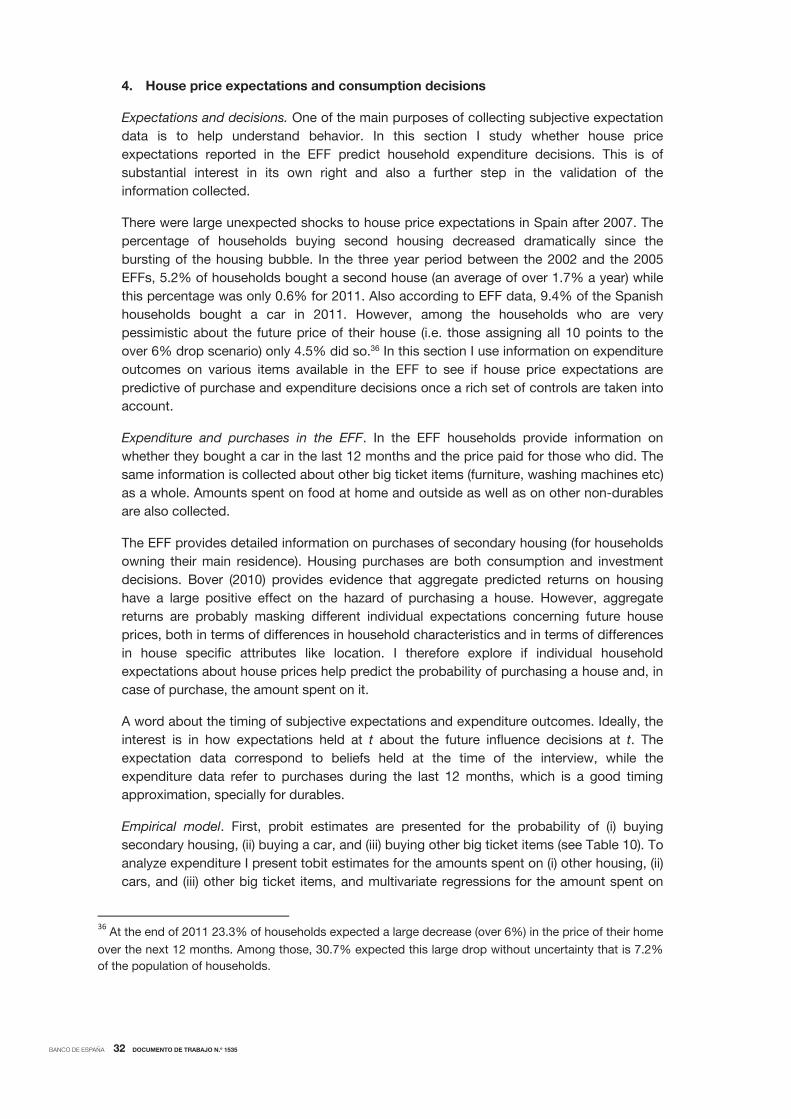
BANCO DE ESPAÑA 32 DOCUMENTO DE TRABAJO N.º 1535
4. House price expectations and consumption decisions
Expectations and decisions. One of the main purposes of collecting subjective expectation
data is to help understand behavior. In this section I study whether house price
expectations reported in the EFF predict household expenditure decisions. This is of
substantial interest in its own right and also a further step in the validation of the
information collected.
There were large unexpected shocks to house price expectations in Spain after 2007. The
percentage of households buying second housing decreased dramatically since the
bursting of the housing bubble. In the three year period between the 2002 and the 2005
EFFs, 5.2% of households bought a second house (an average of over 1.7% a year) while
this percentage was only 0.6% for 2011. Also according to EFF data, 9.4% of the Spanish
households bought a car in 2011. However, among the households who are very
pessimistic about the future price of their house (i.e. those assigning all 10 points to the
over 6% drop scenario) only 4.5% did so.36 In this section I use information on expenditure
outcomes on various items available in the EFF to see if house price expectations are
predictive of purchase and expenditure decisions once a rich set of controls are taken into
account.
Expenditure and purchases in the EFF. In the EFF households provide information on
whether they bought a car in the last 12 months and the price paid for those who did. The
same information is collected about other big ticket items (furniture, washing machines etc)
as a whole. Amounts spent on food at home and outside as well as on other non-durables
are also collected.
The EFF provides detailed information on purchases of secondary housing (for households
owning their main residence). Housing purchases are both consumption and investment
decisions. Bover (2010) provides evidence that aggregate predicted returns on housing
have a large positive effect on the hazard of purchasing a house. However, aggregate
returns are probably masking different individual expectations concerning future house
prices, both in terms of differences in household characteristics and in terms of differences
in house specific attributes like location. I therefore explore if individual household
expectations about house prices help predict the probability of purchasing a house and, in
case of purchase, the amount spent on it.
A word about the timing of subjective expectations and expenditure outcomes. Ideally, the
interest is in how expectations held at t about the future influence decisions at t. The
expectation data correspond to beliefs held at the time of the interview, while the
expenditure data refer to purchases during the last 12 months, which is a good timing
approximation, specially for durables.
Empirical model. First, probit estimates are presented for the probability of (i) buying
secondary housing, (ii) buying a car, and (iii) buying other big ticket items (see Table 10). To
analyze expenditure I present tobit estimates for the amounts spent on (i) other housing, (ii)
cars, and (iii) other big ticket items, and multivariate regressions for the amount spent on
36At the end of 2011 23.3% of households expected a large decrease (over 6%) in the price of their home
over the next 12 months. Among those, 30.7% expected this large drop without uncertainty that is 7.2%
of the population of households.

BANCO DE ESPAÑA 33 DOCUMENTO DE TRABAJO N.º 1535
(iv) food and other non durables (see Table 11A). As is well-known, tobit estimates rely on
the assumption that the same relationship holds both for the decision to purchase and for
the amount spent. To check how restrictive this assumption is here the implied tobit
estimates for the various purchase probabilities are also be provided (see Table 11B) and
compared with the probit estimates.
In the empirical models I include two variables measuring household beliefs about future
house prices. To reflect the location of those expectations, a 0/1 dummy is defined taking
the value 1 for people expecting a large certain drop with certainty (i.e. people who assign
all 10 points to the option “more than 6%” drop). To capture uncertainty about the
expectation location another 0/1 dummy is defined taking the value 1 for respondents
assigning points to more than one option. Note that these indicators are constructed
directly from the household responses, and not from fitted individual probability
distributions.
A potential concern of reverse causality is that the uncertainty about the future price of the
main residence may be reduced by investment in information associated with the purchase
of other housing. However, the results in Table 6 indicate a lack of association between
uncertainty and having bought the main residence recently, which suggests that
endogenous reductions in uncertainty may not be very important.
Importantly, I am able to control for expectations about future household income and
hence identify house price expectations net of income expectations. In the EFF2011
expectations about future household income are collected albeit in a qualitative way.
Households are asked whether, compared to their current income, they believe their
income in the future will be higher, lower, or approximately the same. Two indicators are
constructed containing such that information. 37
Additionally, the occurrence of positive or negative income shocks is controlled for by
exploiting the information provided by a question in the EFF on whether current household
income is higher than usual, lower than usual or as usual.
Other variables included in the estimated models are: log net household wealth and its
interactions with the house price expectations dummies, respondent gender, age (six
interval variables), number of persons in the household (six 0/1 dummies), couple dummy,
children dummy, labour status dummies for respondent (four categories) and partner (if
any).
Regarding location variables two sets of results are presented: controlling for municipality
size (seven categories) or by postal code. However, probit estimates controlling for postal
codes rely on a significantly reduced number of observations because of the requirement
of observing households who buy and households who do not buy at postal code level
(columns 2, 4, and 6 in Table 10). Those results therefore cannot be taken as
representative of the population of households. This is not the case for the tobit estimates
in Tables 11A and 11B.
Results. The results in Table 10 (column 1) show that the most pessimistic households
have a significantly lower probability of buying a house than the rest. The reduction in
37Starting from the 2014 wave the EFF includes a question on probabilistic expectations about future
total household income.

BANCO DE ESPAÑA 34 DOCUMENTO DE TRABAJO N.º 1535
probability is of 0.8 percentage point at the median level of wealth but higher (1.24 pp) at
the 80th wealth percentile. Uncertainty about the evolution of future house prices is also
associated with reductions in the probability of buying a house. The magnitude of this
reduction is 0.63 pp at the median and 0.8 at the 80th percentile. Larger effects at the top
of the wealth distribution appear sensible as those are the households most prone to
buying second housing.
Expecting a large drop in house prices is also associated with a 4.5 pp smaller probability
of buying a car at the median level of wealth but not for wealthier households. However,
uncertain expectations are positively correlated with the probability of buying a car and,
mostly, with other big ticket items. These results could reflect some substitution effects.
Table 11A shows the estimates for the various expenditures. Again, the larger and most
significant effects are the reduction in the amounts spent when buying second housing for
households expecting a large drop in the price of their house or for those being uncertain
about the evolution of the value of their home. For these households the amounts spent
when buying a car are also significantly lower (-13,000 € at median wealth). These
conclusions hold when postal code dummies are included.
Similarly to the results on purchase probabilities, there seem to be some evidence of some
substitution effects for expenditures on other big ticket items and on food and other non-
durables among wealthy households uncertain about future house prices. However, these
results do not hold when controlling for postal code.
Finally, Table 11B reports the probabilities of purchase of the various items obtained from
the tobit model. These are very much in line with those obtained with the probit model (see
Table 10). Furthermore, in this case estimates of the probabilities controlling for postal
code can be obtained for the whole sample and confirm the results in columns 1, 3, and 5
of Tables 10 and 11B.
BANCO DE ESPAÑA 35 DOCUMENTO DE TRABAJO N.º 1535
5. Conclusions
Household predictive probability distributions play an important role in explaining behavior in
many contexts. Not only the location of these distributions but also the uncertainty with which
households hold their beliefs is relevant. It is therefore important to have at our disposal
measures of such probabilistic expectations directly collected from households.
In this paper I have first reviewed recent work about expectations elicited in household
surveys. In particular, I have described relevant implementation specificities as well as
reviewed various uses of subjective probabilistic expectation questions.
Second, I have analyzed the answers to a question recently introduced in the EFF on
probabilistic house price expectations. This analysis shows that asking such type of questions
to Spanish households is feasible (as long as respondents are familiar with the subject matter),
as shown by the high response rate and the results of a coherency analysis.
The results show significant heterogeneity in house price expectations across respondents.
Heterogeneity is found to be significant both for the location of such expectations as well as
for the amount of uncertainty around them. I find that women and blue collar workers are more
optimistic about the evolution of house prices for 2012, and older respondents are more
certain.
The results also provide valuable information about heterogeneity in the housing market.
Location of the house at the postal code level is shown to explain most of the observed
heterogeneity in expectations. Moreover, past returns to housing and unemployment rates are
found to be strong determinants of the estimated effects of location.
Furthermore, the results show that in the absence of controlling for detailed location
information about the house the estimated effects of demographic characteristics on house
price expectations are biased and misleading.
I also exploit the availability of information about various durable and non-durable expenditures
in the EFF and present some novel findings about the association between house price
probabilistic expectations (location and uncertainty) and various durable expenditures. The
results show that households holding pessimistic expectations have significantly lower
probabilities of buying a house and of buying a car. Moreover, the amounts spent on those
items by buyers are also smaller than in the absence of such negative expectations. However, I
find no association between house price expectations and expenditure on other big ticket
items, nor on food and other nondurable expenditure.
Finally, greater uncertainty in house price expectations is associated with a lower probability of
buying a secondary house (as well as with smaller amounts spent) but not with the purchase or
the amount spent in other goods.

BANCO DE ESPAÑA 36 DOCUMENTO DE TRABAJO N.º 1535
REFERENCES
Abadie, A., and G. Imbens (2006): “Large Sample Properties of Matching Estimators for
Average Treatment Effects,” Econometrica, Vol. 74, pp. 235–267.
Armantier, O., Bruine de Bruin, W., Potter, S., Topa, G., van der Klaauw, W. and B. Zafar
(2013): Measuring Inflation Expectations, Annual Review of Economics, vol. 5(1), pp. 273-301
Arrondel, L. Calvo-Pardo, H., and D. Tas (2011): Subjective stock market expectations,
information and stock market participation: evidence from France, mimeo.
Attanasio, O. (2009): Expectations and perceptions in developing countries: their measurement
and their use, American Economic Review: Papers and Proceedings, vol. 99, pp. 87-92.
Attanasio, O. and B. Augsburg (2012): Subjective expectations and income process in rural
India, mimeo.
Balasuriya, J., Muradoglu, G. and P. Ayton (2010): Optimism and portfolio choice, mimeo.
Benítez-Silva, H., Dwyer, D. S., Gayle, W., and T. J. Muench (2008): Expectations in Micro
Data: Rationality Revisited, Empirical Economics, vol. 34, nº 2, pp.381-416
Blanchflower, D. G. and C. MacCoille (2009): The formation of inflation expectations: an
empirical analysis for the UK, NBER Working Paper Nº 15388
Bover, O. (2010): Housing Purchases and the Dynamics of Housing Wealth, CEPR Discussion
Paper Nº 8128, Banco de España Working Paper 1036
Bruine de Bruin, W., van der Klaauw, W., Downs, J., Fischhoff, B., Topa, G. and O. Armantier
(2010): Expectations of inflation: the role of demographic variables, expectation formation, and
financial literacy, The Journal of Consumer Affairs, vol. 44, nº 2, pp. 381-402
Bruine de Bruin, W., Manski, C.F., Topa, G., and W. Van der Klaauw (2011a): Measuring
consumer uncertainty about future inflation, Journal of Applied Econometrics, vol. 26, pp. 454-
478
Bruine de Bruin, W., van der Klaauw, W., and G. Topa (2011b): Expectations of inflation: the
biasing effect of thoughts about specific prices, Journal of Economic Psychology, vol. 32, pp.
834-845
Bruine de Bruin, W., van der Klaauw, W., Downs, J., Fischhoff, B., Topa, G. and O. Armantier
(2012): The effect of question wording on reported expectations and perceptions of inflation,
Journal of Economic Psychology, vol. 33, pp. 749-757
Carroll, C. D. (2003): Macroeconomic Expectations of Households and Professional
Forecasters, Quarterly, Quarterly Journal of Economics, vol.118, nº1, pp.269-298
Case, K. E., Shiller R. J., and A. Thompson (2012): What have they been thinking? Home buyer
behavior in hot and cold markets, NBER Working Paper Nº 18400
Cavallo, A., Cruces, G. and R. Pérez-Truglia (2014): Inflation expectations, learning and
supermarket prices: evidence from field experiments, NBER WP 20576.
Das, M. And B. Donkers (1999): How certain are Dutch households about future income? An
empirical analysis, Review of Income and Wealth, vol. 45, nº 3, pp. 325-338

BANCO DE ESPAÑA 37 DOCUMENTO DE TRABAJO N.º 1535
Delavande, A. Giné, X. and D. McKenzie (2011): Eliciting probabilistic expectations with visual
aids in developing countries: how sensitive are answers to variations in elicitation design?,
Journal of Applied Econometrics, vol. 26, pp.479-497
Delavande, A. and S. Rohwedder (2011): Individuals’ uncertainty about future social security
benefits and portfolio choice, Journal of Applied Econometrics, vol. 26, pp. 498-519
Dominitz, J. and C. F. Manski (1997): Using expectations data to study subjective income
expectations, Journal of the American Statistical Association, vol. 92, nº 439, pp. 855-867
Dominitz, J. and C. F. Manski (2004): How should we measure consumer confidence?, Journal
of Economic Perspectives, vol. 18, nº 2, pp. 51-66
Dominitz, J. and C. F. Manski (2007): Expected equity returns and portfolio choice: evidence
from the Health and Retirement Study, Journal of the European Economic Association, vol. 5,
nº 2/3, Papers and Proceedings, pp. 369-379
Fischhoff, B. and W. Bruine de Bruin (1999): Fifty-fifty=50%? Journal of Behavioral Decision
Making, vol. 12, pp. 149-163
Gan L., Gong G., Hurd M., and D. McFadden (2004): Subjective mortality risk and bequests,
NBER Working Paper No. 10789
Gouret, F. And G. Hollard (2011): When Kahneman meets Manksi: using dual systems of
reasoning to interpret subjective expectations of equity returns, Journal of Applied
Econometrics, 26, pp. 371-392
Hudomiet, P., Kézdi, G. and R. J. Willis (2011): Stock market crash and expectations of
American households, Journal of Applied Econometrics, vol. 26, pp. 393-415
Hurd, M. (2009): Subjective probabilities in household surveys, Annual Review of Economics,
vol.1, pp. 543-562
Hurd, M., McFadden, D. and L. Gan (1998): “Subjective Survival Curves and Life Cycle Saving
Behavior.” In David Wise, ed., Inquiries in the Economics of Aging. The University of Chicago
Press, pp. 259-305.
Hurd M., Smith J., and J. Zissimopoulos (2004): The effects of subjective survival on retirement
and Social Security claiming, Journal of Applied Econometrics, 19, pp. 761–75
Hurd, M. D., van Rooij, M. and J. Winter (2011): Stock market expectations of Dutch
households, Journal of Applied Econometrics, 26, pp. 416-436
Juster, F. T. (1964): Anticipations and Purchases: An Analysis of Consumer Behavior, Princeton
University Press.
Juster, F. T.(1966): Consumer Buying Intentions and Purchase Probability: An Experiment in
Survey Design, Journal of the American Statistical Association, vol. 61, pp. 658-696
Katona, G. (1957): Federal Reserve Board Committee Reports on Consumer Expectations and
Savings Statistics, Review of Economics and Statistics, vol. 39, pp. 40-46
Kézdi, G. and J. Willis (2008): Stock market expectations and portfolio choice of American
households, mimeo

BANCO DE ESPAÑA 38 DOCUMENTO DE TRABAJO N.º 1535
Lillard, L. A. and R. J. Willis (2001): Cognition and wealth: the importance of probabilistic
thinking, mimeo.
Lucas, R. E. (1973): Some International Evidence on Output-Inflation Tradeoffs, American
Economic Review, vol. 63, pp. 326-34
Malmendier, U. And S. Nagel (2013): Learning from inflation experiences, mimeo.
Mankiw, N. G., Reis, R. and J. Wolfers (2003): Disagreement about inflation expectations,
NBER Working Paper Nº 9796
Manski, C. F. (2004): Measuring expectations, Econometrica, vol. 72, nº5, pp. 1329-1376
Morgan, G., and M. Henrion (1990): Uncertainty: A Guide to Dealing with Uncertainty in
Quantitative Risk and Policy Analysis, New York: Cambridge University Press.
Niu, G. and A. van Soest (2014): House price expectations, IZA DP Nº 8536.
Pesaran, H. and M. Weale (2006): Survey expectations, in Handbook of Econometric
Forecasting, G. Elliott, C.W. Granger, and A. Timmermann (eds.), vol.1, pp.715-776, North
Holland
Phelps, E. S. (1970), Money-Wage Dynamics and Labor-Market Equilibrium, in E. S Phelps et
al., Microeconomic Foundations of Employment and Inflation Theory, New York: Norton.
Ranyard, R., Del Missier, F., Bonini, N., Duxbury, D. And B. Summers (2008): Perceptions and
expectations of price changes and inflation: A review and conceptual work, Journal of
Economic Psychology, vol. 29, pp. 378-400.
Slovic, P., Finucane, M., Peters, E. And D. MacGregor (2001): The affect heuristic, in T.
Gilovich, D. Griffin, and D. Kahneman, eds, Heuristic and biases: The psychology of intuitive
judgment, pp. 397-420, New York, Cambridge University Press.
Souleles, N. S. (2004): Expectations, heterogeneous forecast errors and consumption: micro
evidence from the Michigan Consumer Sentiment Survey, Journal of Money, Credit and
Banking, vol. 36, pp.39-72.
Tetlock, Ph. and D. Gardner (2015): Superforecasting: The Art and Science of Prediction,
Random House Books.
Tversky, A. and D. Kahneman (1974): Judgement under uncertainty: heuristics and biases,
Science, vol. 185, pp. 1124-113
van der Klaauw, W., Bruine de Bruin, W., Topa, G., Potter, S., and M. Bryan (2008): Rethinking
the measurement of household inflation expectations: preliminary findings, Federal Reserve
Bank of New York Staff Report nº 359
Winter, J. (2008): Expectations and attitudes, Expectations and attitudes, in: A. Borsch-Supan,
A. Brugiavini, H. Jurges, A. Kapteyn, J. Mackenbach, J. Siegrist, G. Weber, eds., First Results
from the Survey of Health, Ageing and Retirement in Europe 2004-2007, pp. 306-11.
Mannheim: Mannheim Research Institute for the Economics of Aging
Zafar, B. (2011): Can subjective expectations data be used in choice models? Evidence on
cognitive biases, Journal of Applied Econometrics, vol. 26, pp. 520-544
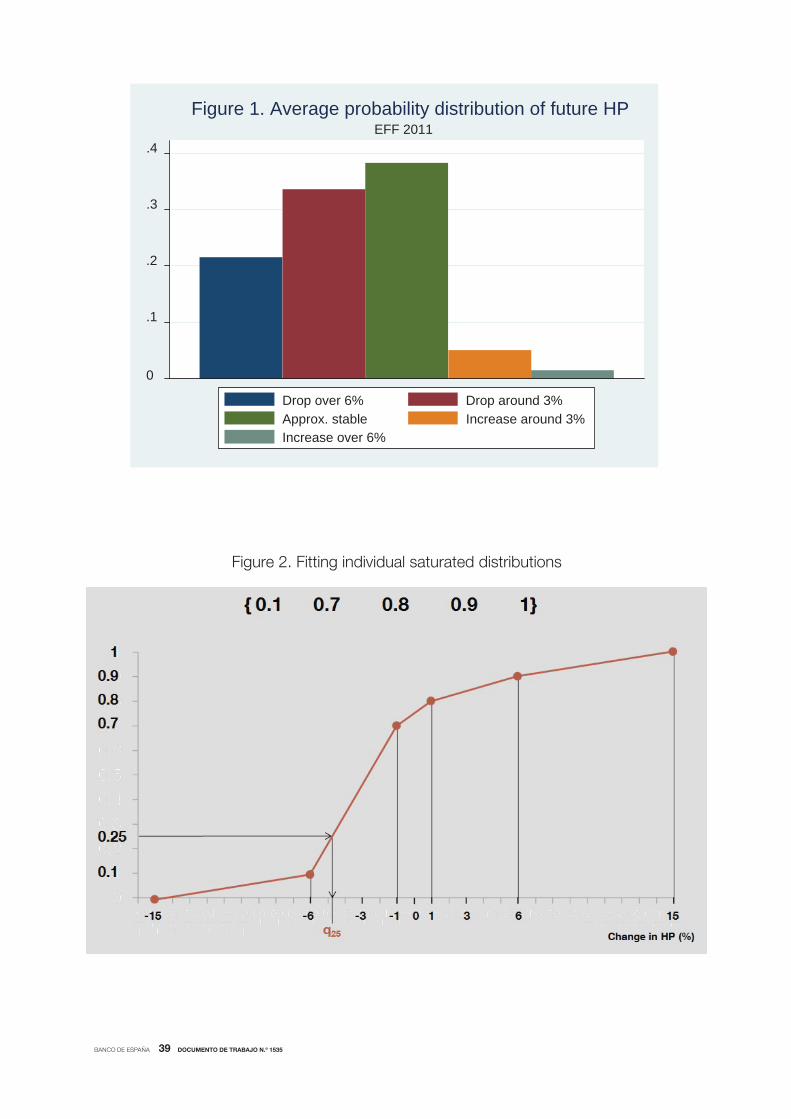
BANCO DE ESPAÑA 39 DOCUMENTO DE TRABAJO N.º 1535
0
.1
.2
.3
.4EFF 2011
Figure 1. Average probability distribution of future HP
Drop over 6% Drop around 3%Approx. stable Increase around 3% Increase over 6%
Figure 2. Fitting individual saturated distributions
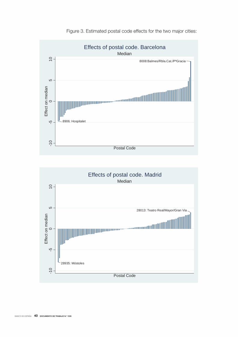
BANCO DE ESPAÑA 40 DOCUMENTO DE TRABAJO N.º 1535
Figure 3. Estimated postal code effects for the two major cities:
8906: Hospitalet
8008:Balmes/Rbla.Cat./PºGracia
-10
-50
510
Effe
ct o
n m
edia
n
Postal Code
MedianEffects of postal code. Barcelona
28013: Teatro Real/Mayor/Gran Via
28935: Móstoles
-10
-50
510
Effe
ct o
n m
edia
n
Postal Code
MedianEffects of postal code. Madrid
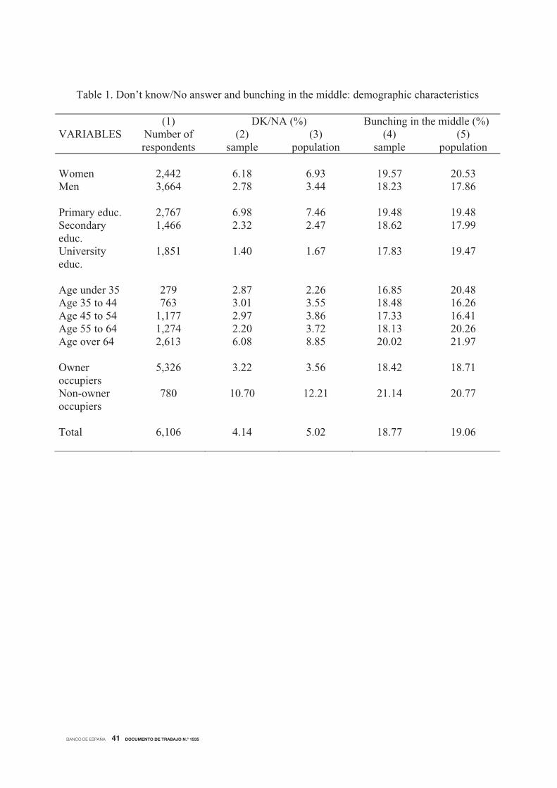
BANCO DE ESPAÑA 41 DOCUMENTO DE TRABAJO N.º 1535
Table 1. Don’t know/No answer and bunching in the middle: demographic characteristics
(1) Number of respondents
DK/NA (%) Bunching in the middle (%) VARIABLES (2)
sample (3)
population(4)
sample (5)
population Women 2,442 6.18 6.93 19.57 20.53 Men 3,664 2.78 3.44 18.23 17.86 Primary educ. 2,767 6.98 7.46 19.48 19.48 Secondaryeduc.
1,466 2.32 2.47 18.62 17.99
Universityeduc.
1,851 1.40 1.67 17.83 19.47
Age under 35 279 2.87 2.26 16.85 20.48 Age 35 to 44 763 3.01 3.55 18.48 16.26 Age 45 to 54 1,177 2.97 3.86 17.33 16.41 Age 55 to 64 1,274 2.20 3.72 18.13 20.26 Age over 64 2,613 6.08 8.85 20.02 21.97 Owneroccupiers
5,326 3.22 3.56 18.42 18.71
Non-owneroccupiers
780 10.70 12.21 21.14 20.77
Total 6,106 4.14 5.02 18.77 19.06
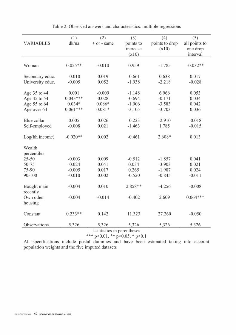
BANCO DE ESPAÑA 42 DOCUMENTO DE TRABAJO N.º 1535
Table 2. Observed answers and characteristics: multiple regressions
(1) (2) (3) (4) (5) VARIABLES dk/na + or - same points to
increase (x10)
points to drop (x10)
all points to one drop interval
Woman 0.025** -0.010 0.959 -1.785 -0.032** Secondary educ. -0.010 0.019 -0.661 0.638 0.017 University educ. -0.005 0.052 -1.938 -2.218 -0.028 Age 35 to 44 0.001 -0.009 -1.148 6.966 0.053 Age 45 to 54 0.043*** 0.028 -0.694 -0.171 0.034 Age 55 to 64 0.034* 0.086* -1.906 -3.583 0.042 Age over 64 0.061*** 0.081* -3.105 -3.703 0.036 Blue collar 0.005 0.026 -0.223 -2.910 -0.018 Self-employed -0.008 0.021 -1.463 1.785 -0.015 Log(hh income) -0.020** 0.002 -0.461 2.608* 0.013 Wealth percentiles
25-50 -0.003 0.009 -0.512 -1.857 0.041 50-75 -0.024 0.041 0.034 -3.903 0.021 75-90 -0.005 0.017 0.265 -1.987 0.024 90-100 -0.010 0.002 -0.520 -0.845 -0.011 Bought main recently
-0.004 0.010 2.858** -4.256 -0.008
Own other housing
-0.004 -0.014 -0.402 2.609 0.064***
Constant 0.233** 0.142 11.323 27.260 -0.050 Observations 5,326 5,326 5,326 5,326 5,326
t-statistics in parentheses *** p<0.01, ** p<0.05, * p<0.1
All specifications include postal dummies and have been estimated taking into account population weights and the five imputed datasets

BANCO DE ESPAÑA 43 DOCUMENTO DE TRABAJO N.º 1535
Table 3. Bins used (%)
Nº of bins used Sample Population 1 38.55 36.17 2 33.62 35.01 3 17.13 16.26 4 4.37 5.31 5 6.32 7.24
Using non-adjacent bins 1.59 1.66

BANCO DE ESPAÑA 44 DOCUMENTO DE TRABAJO N.º 1535
Table 4. Most frequent answers to probabilistic expectations of future house prices
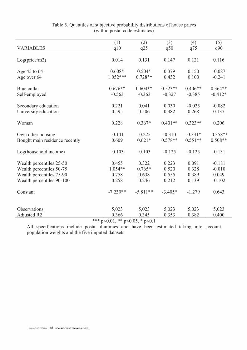
BANCO DE ESPAÑA 45 DOCUMENTO DE TRABAJO N.º 1535
Table 5. Quantiles of subjective probability distributions of house prices (within postal code estimates)
(1) (2) (3) (4) (5) VARIABLES q10 q25 q50 q75 q90 Log(price/m2) 0.014 0.131 0.147 0.121 0.116 Age 45 to 64 0.608* 0.504* 0.379 0.150 -0.087 Age over 64 1.052*** 0.728** 0.432 0.100 -0.241 Blue collar 0.676** 0.604** 0.523** 0.406** 0.364** Self-employed -0.563 -0.363 -0.327 -0.385 -0.412* Secondary education 0.221 0.041 0.030 -0.025 -0.082 University education 0.595 0.506 0.382 0.268 0.137 Woman 0.228 0.367* 0.401** 0.323** 0.206 Own other housing -0.141 -0.225 -0.310 -0.331* -0.358** Bought main residence recently 0.609 0.621* 0.578** 0.551** 0.508** Log(household income) -0.103 -0.103 -0.125 -0.125 -0.131 Wealth percentiles 25-50 0.455 0.322 0.223 0.091 -0.181 Wealth percentiles 50-75 1.054** 0.765* 0.520 0.328 -0.010 Wealth percentiles 75-90 0.758 0.638 0.555 0.389 0.049 Wealth percentiles 90-100 0.258 0.246 0.212 0.139 -0.102 Constant -7.230** -5.811** -3.405* -1.279 0.643 Observations 5,023 5,023 5,023 5,023 5,023 Adjusted R2 0.366 0.345 0.353 0.382 0.400
*** p<0.01, ** p<0.05, * p<0.1 All specifications include postal dummies and have been estimated taking into account population weights and the five imputed datasets
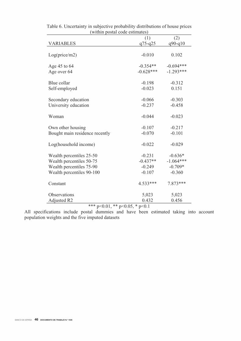
BANCO DE ESPAÑA 46 DOCUMENTO DE TRABAJO N.º 1535
Table 6. Uncertainty in subjective probability distributions of house prices (within postal code estimates)
(1) (2) VARIABLES q75-q25 q90-q10 Log(price/m2) -0.010 0.102 Age 45 to 64 -0.354** -0.694*** Age over 64 -0.628*** -1.293***
Blue collar -0.198 -0.312 Self-employed -0.023 0.151 Secondary education -0.066 -0.303 University education -0.237 -0.458 Woman -0.044 -0.023 Own other housing -0.107 -0.217 Bought main residence recently -0.070 -0.101 Log(household income) -0.022 -0.029 Wealth percentiles 25-50 -0.231 -0.636* Wealth percentiles 50-75 -0.437** -1.064*** Wealth percentiles 75-90 -0.249 -0.709* Wealth percentiles 90-100 -0.107 -0.360 Constant 4.533*** 7.873*** Observations 5,023 5,023 Adjusted R2 0.432 0.456
*** p<0.01, ** p<0.05, * p<0.1 All specifications include postal dummies and have been estimated taking into account population weights and the five imputed datasets
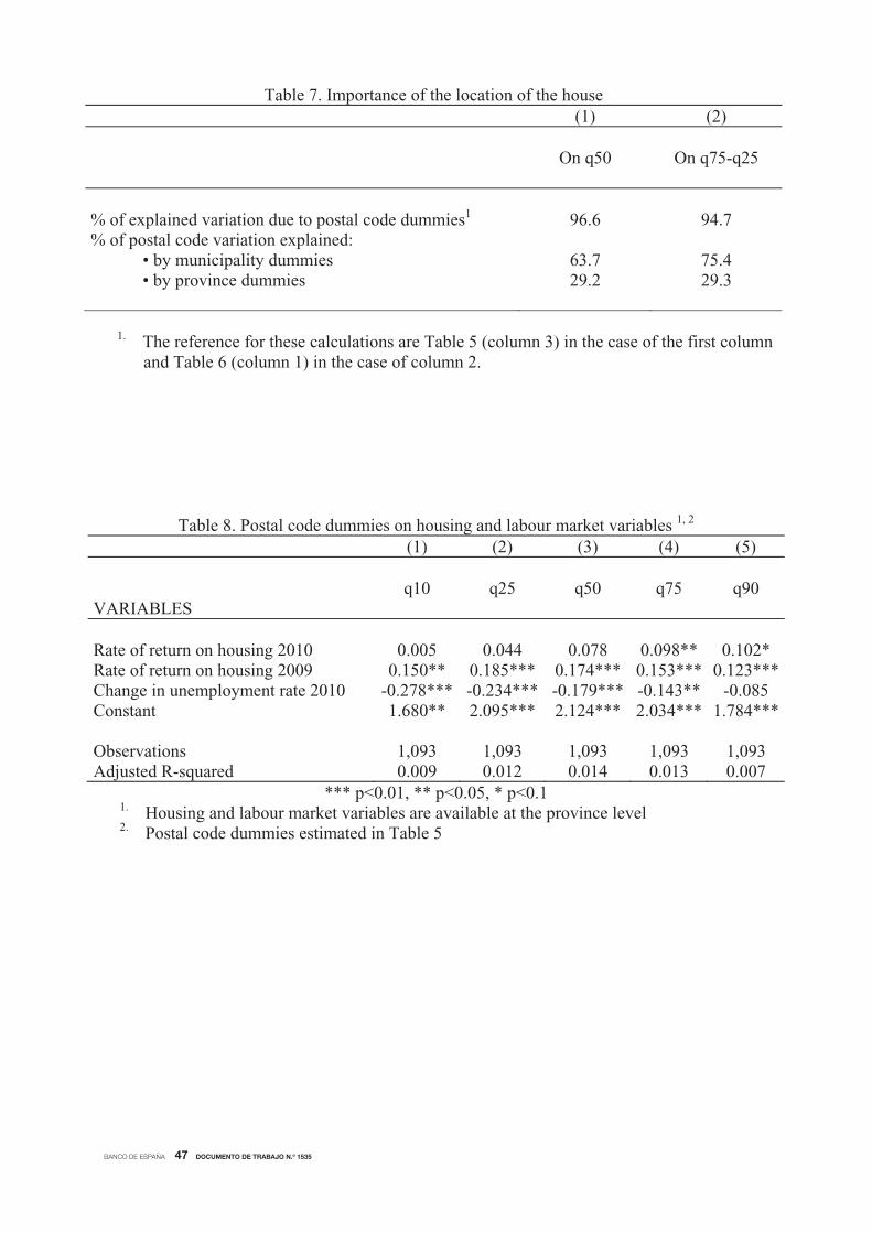
BANCO DE ESPAÑA 47 DOCUMENTO DE TRABAJO N.º 1535
Table 7. Importance of the location of the house (1) (2) On q50 On q75-q25 % of explained variation due to postal code dummies1 96.6 94.7 % of postal code variation explained:
• by municipality dummies 63.7 75.4 • by province dummies 29.2 29.3
1. The reference for these calculations are Table 5 (column 3) in the case of the first column and Table 6 (column 1) in the case of column 2.
Table 8. Postal code dummies on housing and labour market variables 1, 2
(1) (2) (3) (4) (5) q10 q25 q50 q75 q90 VARIABLES Rate of return on housing 2010 0.005 0.044 0.078 0.098** 0.102* Rate of return on housing 2009 0.150** 0.185*** 0.174*** 0.153*** 0.123***Change in unemployment rate 2010 -0.278*** -0.234*** -0.179*** -0.143** -0.085 Constant 1.680** 2.095*** 2.124*** 2.034*** 1.784*** Observations 1,093 1,093 1,093 1,093 1,093 Adjusted R-squared 0.009 0.012 0.014 0.013 0.007
*** p<0.01, ** p<0.05, * p<0.1 1. Housing and labour market variables are available at the province level2. Postal code dummies estimated in Table 5

BANCO DE ESPAÑA 48 DOCUMENTO DE TRABAJO N.º 1535
Table 9. Postal code dummies on housing and labour market variables 1, 2
(1) (2) q75-q25 q90-q10 VARIABLES Change in rate of return on housing 2010 0.042* 0.029 Change in unemployment rate 2010 0.097** 0.114*** Constant -0.210* -3.307*** Observations 1,093 1,093 Adjusted R-squared 0.006 0.006
*** p<0.01, ** p<0.05, * p<0.11. Housing and labour market variables are available at the province level2. Postal code dummies estimated in Table 6
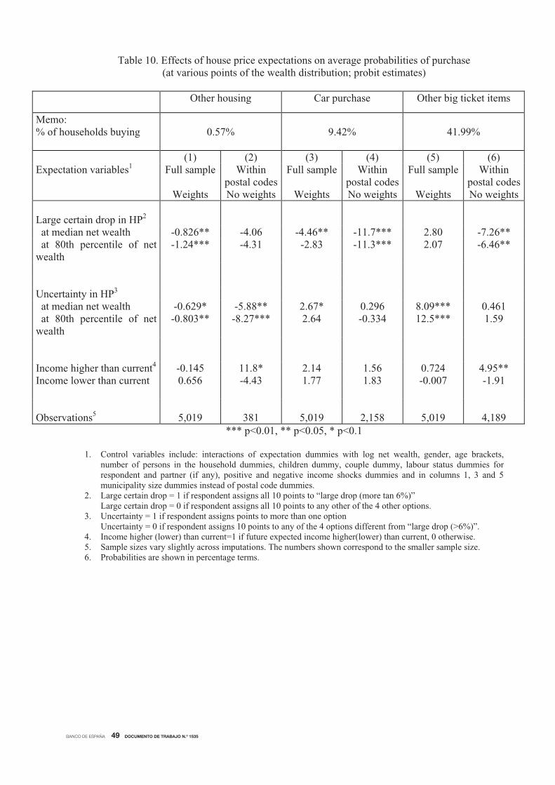
BANCO DE ESPAÑA 49 DOCUMENTO DE TRABAJO N.º 1535
Table 10. Effects of house price expectations on average probabilities of purchase(at various points of the wealth distribution; probit estimates)
Other housing Car purchase Other big ticket items
Memo: % of households buying 0.57% 9.42% 41.99%
(1) (2) (3) (4) (5) (6) Expectation variables1 Full sample
Weights
Within postal codesNo weights
Full sample
Weights
Within postal codes No weights
Full sample
Weights
Within postal codesNo weights
Large certain drop in HP2
at median net wealth -0.826** -4.06 -4.46** -11.7*** 2.80 -7.26** at 80th percentile of net wealth
-1.24*** -4.31 -2.83 -11.3*** 2.07 -6.46**
Uncertainty in HP3
at median net wealth -0.629* -5.88** 2.67* 0.296 8.09*** 0.461 at 80th percentile of net wealth
-0.803** -8.27*** 2.64 -0.334 12.5*** 1.59
Income higher than current4 -0.145 11.8* 2.14 1.56 0.724 4.95** Income lower than current 0.656 -4.43 1.77 1.83 -0.007 -1.91 Observations5 5,019 381 5,019 2,158 5,019 4,189
*** p<0.01, ** p<0.05, * p<0.1
1. Control variables include: interactions of expectation dummies with log net wealth, gender, age brackets, number of persons in the household dummies, children dummy, couple dummy, labour status dummies for respondent and partner (if any), positive and negative income shocks dummies and in columns 1, 3 and 5 municipality size dummies instead of postal code dummies.
2. Large certain drop = 1 if respondent assigns all 10 points to “large drop (more tan 6%)” Large certain drop = 0 if respondent assigns all 10 points to any other of the 4 other options.
3. Uncertainty = 1 if respondent assigns points to more than one option Uncertainty = 0 if respondent assigns 10 points to any of the 4 options different from “large drop (>6%)”.
4. Income higher (lower) than current=1 if future expected income higher(lower) than current, 0 otherwise. 5. Sample sizes vary slightly across imputations. The numbers shown correspond to the smaller sample size. 6. Probabilities are shown in percentage terms.
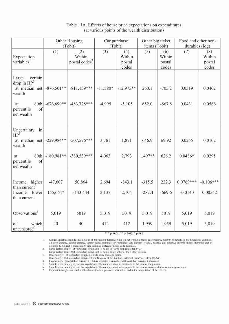
BANCO DE ESPAÑA 50 DOCUMENTO DE TRABAJO N.º 1535
Table 11A. Effects of house price expectations on expenditures(at various points of the wealth distribution)
Other Housing (Tobit)
Car purchase (Tobit)
Other big ticket items (Tobit)
Food and other non-durables (log)
(1) (2) (3) (4) (5) (6) (7) (8) Expectationvariables1
Within postal codes7
Within postalcodes
Within postalcodes
Within postalcodes
Large certain drop in HP2
at median net wealth
-876,501** -811,159*** -11,580* -12,975** 260.1 -705.2 0.0319 0.0402
at 80th percentile of net wealth
-676,699** -483,728*** -4,995 -5,105 652.0 -667.8 0.0431 0.0566
Uncertainty in HP3
at median net wealth
-229,984** -507,576*** 3,761 1,871 646.9 69.92 0.0255 0.0102
at 80th percentile of net wealth
-180,981** -380,539*** 4,063 2,793 1,497** 626.2 0.0486* 0.0295
Income higher than current4
-47,607 50,864 2,694 -843.1 -315.5 222.3 0.0769*** -0.106***
Income lower than current
155,664* -143,444 2,137 2,104 -282.4 -669.6 -0.0140 0.00542
Observations5 5,019 5019 5,019 5019 5,019 5019 5,019 5,019
of which uncensored6
40 40 412 412 1,959 1,959 5,019 5,019
*** p<0.01, ** p<0.05, * p<0.1
1. Control variables include: interactions of expectation dummies with log net wealth, gender, age brackets, number of persons in the household dummies, children dummy, couple dummy, labour status dummies for respondent and partner (if any), positive and negative income shocks dummies and in columns 1, 3, 5 and 7 municipality size dummies instead of postal code dummies.
2. Large certain drop = 1 if respondent assigns all 10 points to “large drop (more tan 6%)” Large certain drop = 0 if respondent assigns all 10 points to any other of the 4 other options.
3. Uncertainty = 1 if respondent assigns points to more than one option Uncertainty = 0 if respondent assigns 10 points to any of the 4 options different from “large drop (>6%)”.
4. Income higher (lower) than current=1 if future expected income higher(lower) than current, 0 otherwise. 5. Sample sizes vary slightly across imputations. The numbers shown correspond to the smaller sample size. 6. Sample sizes vary slightly across imputations. The numbers shown correspond to the smaller number of uncensored observations. 7. Population weights are used in all columns (both in parameter estimation and in the computation of the effects).
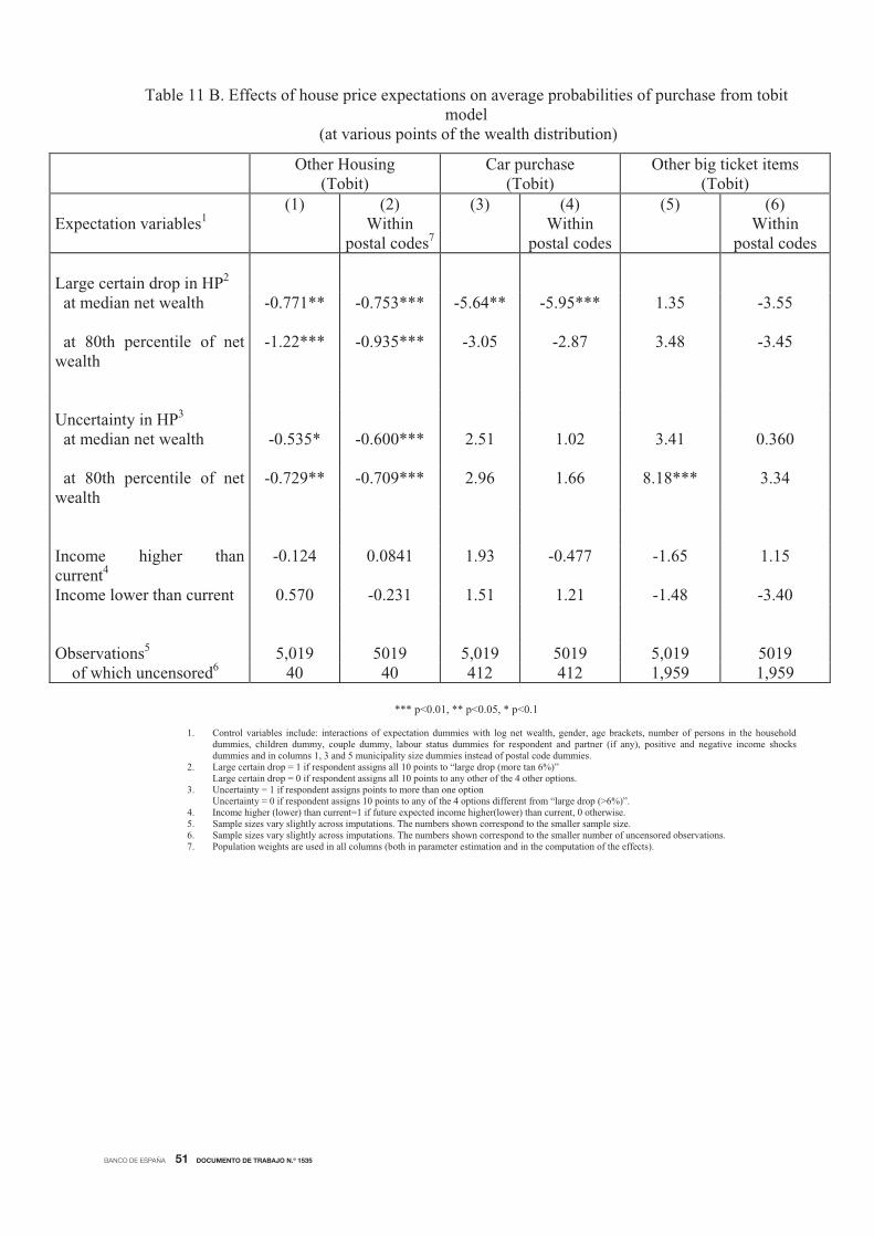
BANCO DE ESPAÑA 51 DOCUMENTO DE TRABAJO N.º 1535
Table 11 B. Effects of house price expectations on average probabilities of purchase from tobit model
(at various points of the wealth distribution)
*** p<0.01, ** p<0.05, * p<0.1
1. Control variables include: interactions of expectation dummies with log net wealth, gender, age brackets, number of persons in the household dummies, children dummy, couple dummy, labour status dummies for respondent and partner (if any), positive and negative income shocks dummies and in columns 1, 3 and 5 municipality size dummies instead of postal code dummies.
2. Large certain drop = 1 if respondent assigns all 10 points to “large drop (more tan 6%)” Large certain drop = 0 if respondent assigns all 10 points to any other of the 4 other options.
3. Uncertainty = 1 if respondent assigns points to more than one option Uncertainty = 0 if respondent assigns 10 points to any of the 4 options different from “large drop (>6%)”.
4. Income higher (lower) than current=1 if future expected income higher(lower) than current, 0 otherwise. 5. Sample sizes vary slightly across imputations. The numbers shown correspond to the smaller sample size. 6. Sample sizes vary slightly across imputations. The numbers shown correspond to the smaller number of uncensored observations. 7. Population weights are used in all columns (both in parameter estimation and in the computation of the effects).
Other Housing (Tobit)
Car purchase (Tobit)
Other big ticket items (Tobit)
(1) (2) (3) (4) (5) (6) Expectation variables1 Within
postal codes7 Within
postal codes Within
postal codes Large certain drop in HP2 at median net wealth -0.771** -0.753*** -5.64** -5.95*** 1.35 -3.55
at 80th percentile of net wealth
-1.22*** -0.935*** -3.05 -2.87 3.48 -3.45
Uncertainty in HP3 at median net wealth -0.535* -0.600*** 2.51 1.02 3.41 0.360
at 80th percentile of net wealth
-0.729** -0.709*** 2.96 1.66 8.18*** 3.34
Income higher than current4
-0.124 0.0841 1.93 -0.477 -1.65 1.15
Income lower than current 0.570 -0.231 1.51 1.21 -1.48 -3.40 Observations5 5,019 5019 5,019 5019 5,019 5019 of which uncensored6 40 40 412 412 1,959 1,959
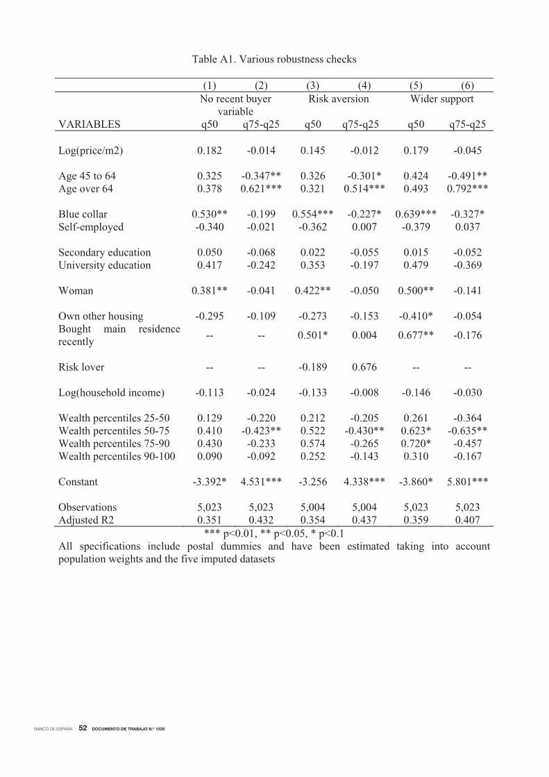
BANCO DE ESPAÑA 52 DOCUMENTO DE TRABAJO N.º 1535
Table A1. Various robustness checks
(1) (2) (3) (4) (5) (6) No recent buyer
variableRisk aversion Wider support
VARIABLES q50 q75-q25 q50 q75-q25 q50 q75-q25 Log(price/m2) 0.182 -0.014 0.145 -0.012 0.179 -0.045 Age 45 to 64 0.325 -0.347** 0.326 -0.301* 0.424 -0.491** Age over 64 0.378 0.621*** 0.321 0.514*** 0.493 0.792*** Blue collar 0.530** -0.199 0.554*** -0.227* 0.639*** -0.327* Self-employed -0.340 -0.021 -0.362 0.007 -0.379 0.037 Secondary education 0.050 -0.068 0.022 -0.055 0.015 -0.052 University education 0.417 -0.242 0.353 -0.197 0.479 -0.369 Woman 0.381** -0.041 0.422** -0.050 0.500** -0.141 Own other housing -0.295 -0.109 -0.273 -0.153 -0.410* -0.054 Bought main residence recently
-- -- 0.501* 0.004 0.677** -0.176
Risk lover -- -- -0.189 0.676 -- -- Log(household income) -0.113 -0.024 -0.133 -0.008 -0.146 -0.030 Wealth percentiles 25-50 0.129 -0.220 0.212 -0.205 0.261 -0.364 Wealth percentiles 50-75 0.410 -0.423** 0.522 -0.430** 0.623* -0.635** Wealth percentiles 75-90 0.430 -0.233 0.574 -0.265 0.720* -0.457 Wealth percentiles 90-100 0.090 -0.092 0.252 -0.143 0.310 -0.167 Constant -3.392* 4.531*** -3.256 4.338*** -3.860* 5.801*** Observations 5,023 5,023 5,004 5,004 5,023 5,023 Adjusted R2 0.351 0.432 0.354 0.437 0.359 0.407
*** p<0.01, ** p<0.05, * p<0.1 All specifications include postal dummies and have been estimated taking into account population weights and the five imputed datasets
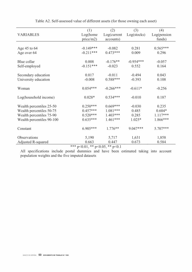
BANCO DE ESPAÑA 53 DOCUMENTO DE TRABAJO N.º 1535
Table A2. Self-assessed value of different assets (for those owning each asset)
(1) (2) (3) (4) VARIABLES Log(home
price/m2) Log(currentaccounts)
Log(stocks) Log(pension funds)
Age 45 to 64 -0.149*** -0.082 0.281 0.565*** Age over 64 -0.211*** 0.473*** 0.009 0.296 Blue collar 0.008 -0.176** -0.954*** -0.057 Self-employed -0.151*** -0.023 0.552 0.164 Secondary education 0.017 -0.011 -0.494 0.043 University education -0.008 0.588*** -0.393 0.108 Woman 0.054*** -0.266*** -0.611* -0.256 Log(household income) 0.028* 0.534*** -0.010 0.187 Wealth percentiles 25-50 0.250*** 0.669*** -0.030 0.235 Wealth percentiles 50-75 0.457*** 1.081*** 0.485 0.604* Wealth percentiles 75-90 0.520*** 1.403*** 0.285 1.117*** Wealth percentiles 90-100 0.635*** 1.461*** 1.025* 1.866*** Constant 6.905*** 1.776** 9.047*** 5.707*** Observations 5,190 5,717 1,631 1,858 Adjusted R-squared 0.663 0.447 0.673 0.584
*** p<0.01, ** p<0.05, ** p<0.1 All specifications include postal dummies and have been estimated taking into account population weights and the five imputed datasets

BANCO DE ESPAÑA 54 DOCUMENTO DE TRABAJO N.º 1535
Table A3. Some quantile measures of subjective probability distributions of house prices:(i) no location information, (ii) municipality dummies
(1) (2) (3) (4) (5) (6) No location information Municipality dummies VARIABLES q25 q50 q75-q25 q25 q50 q75-q25 Log(price/m2) -0.237 -0.074 0.256*** -0.142 -0.019 0.148 Age 45 to 64 0.079 0.113 -0.061 0.281 0.272 -0.157 Age over 64 0.398 0.114 -0.621*** 0.645** 0.481* -0.473*** Blue collar 0.423 0.387* -0.118 0.464* 0.412* -0.188 Self-employed -0.395 -0.444 -0.171 -0.315 -0.217 0.032 Secondary education -0.295 -0.286 -0.009 -0.124 -0.102 -0.028 University education 0.421 0.345 -0.199 0.454 0.396 -0.177 Woman 0.294 0.226 -0.161 0.269 0.313* -0.001 Own other housing -0.102 -0.236 -0.174 -0.123 -0.217 -0.116 Bought main residence recently 0.878** 0.605* -0.437** 0.753** 0.639** -0.166 Log(household income) -0.071 -0.144 -0.108 -0.121 -0.132 -0.021 Wealth percentiles 25-50 0.635 0.221 -0.650*** 0.652* 0.316 -0.471** Wealth percentiles 50-75 1.024** 0.474 -0.833*** 1.056*** 0.583* -0.642***Wealth percentiles 75-90 0.954** 0.425 -0.764*** 0.891** 0.474 -0.531** Wealth percentiles 90-100 0.719 0.304 -0.537* 0.546 0.178 -0.396 Constant -3.939* -1.508 4.314*** 0.723 0.777 0.736 Observations 5,023 5,023 5,023 5,023 5,023 5,023 Adjusted R2 0.0116 0.00988 0.0218 0.208 0.209 0.318
*** p<0.01, ** p<0.05, * p<0.1 All specifications have been estimated taking into account population weights and the five imputed datasets. Columns 1 to 3 include no location dummies and columns 4 to 6 include municipality dummies.

BANCO DE ESPAÑA PUBLICATIONS
WORKING PAPERS
1416 DIEGO J. PEDREGAL, JAVIER J. PÉREZ and A. JESÚS SÁNCHEZ-FUENTES: A toolkit to strengthen government
budget surveillance.
1417 J. IGNACIO CONDE-RUIZ, and CLARA I. GONZÁLEZ: From Bismarck to Beveridge: the other pension reform in Spain.
1418 PABLO HERNÁNDEZ DE COS, GERRIT B. KOESTER, ENRIQUE MORAL-BENITO and CHRISTIANE NICKEL:
Signalling fi scal stress in the euro area: a country-specifi c early warning system.
1419 MIGUEL ALMUNIA and DAVID LÓPEZ-RODRÍGUEZ: Heterogeneous responses to effective tax enforcement:
evidence from Spanish fi rms.
1420 ALFONSO R. SÁNCHEZ: The automatic adjustment of pension expenditures in Spain: an evaluation of the 2013
pension reform.
1421 JAVIER ANDRÉS, ÓSCAR ARCE and CARLOS THOMAS: Structural reforms in a debt overhang.
1422 LAURA HOSPIDO and ENRIQUE MORAL-BENITO: The public sector wage premium in Spain: evidence from
longitudinal administrative data.
1423 MARÍA DOLORES GADEA-RIVAS, ANA GÓMEZ-LOSCOS and GABRIEL PÉREZ-QUIRÓS: The Two Greatest. Great
Recession vs. Great Moderation.
1424 ENRIQUE MORAL-BENITO and OLIVER ROEHN: The impact of fi nancial (de)regulation on current account balances.
1425 MAXIMO CAMACHO and JAIME MARTINEZ-MARTIN: Real-time forecasting US GDP from small-scale factor models.
1426 ALFREDO MARTÍN OLIVER, SONIA RUANO PARDO and VICENTE SALAS FUMÁS: Productivity and welfare: an
application to the Spanish banking industry.
1427 JAVIER ANDRÉS and PABLO BURRIEL: Infl ation dynamics in a model with fi rm entry and (some) heterogeneity.
1428 CARMEN BROTO and LUIS MOLINA: Sovereign ratings and their asymmetric response to fundamentals.
1429 JUAN ÁNGEL GARCÍA and RICARDO GIMENO: Flight-to-liquidity fl ows in the euro area sovereign debt crisis.
1430 ANDRÈ LEMELIN, FERNANDO RUBIERA-MOROLLÓN and ANA GÓMEZ-LOSCOS: Measuring urban agglomeration.
A refoundation of the mean city-population size index.
1431 LUIS DÍEZ-CATALÁN and ERNESTO VILLANUEVA: Contract staggering and unemployment during the Great Recession:
evidence from Spain.
1501 LAURA HOSPIDO and EVA MORENO-GALBIS: The Spanish productivity puzzle in the Great Recession.
1502 LAURA HOSPIDO, ERNESTO VILLANUEVA and GEMA ZAMARRO: Finance for all: the impact of fi nancial literacy training
in compulsory secondary education in Spain.
1503 MARIO IZQUIERDO, JUAN F. JIMENO and AITOR LACUESTA: Spain: from immigration to emigration?
1504 PAULINO FONT, MARIO IZQUIERDO and SERGIO PUENTE: Real wage responsiveness to unemployment in Spain:
asymmetries along the business cycle.
1505 JUAN S. MORA-SANGUINETTI and NUNO GAROUPA: Litigation in Spain 2001-2010: Exploring the market
for legal services.
1506 ANDRES ALMAZAN, ALFREDO MARTÍN-OLIVER and JESÚS SAURINA: Securitization and banks’ capital structure.
1507 JUAN F. JIMENO, MARTA MARTÍNEZ-MATUTE and JUAN S. MORA-SANGUINETTI: Employment protection legislation
and labor court activity in Spain.
1508 JOAN PAREDES, JAVIER J. PÉREZ and GABRIEL PEREZ-QUIRÓS: Fiscal targets. A guide to forecasters?
1509 MAXIMO CAMACHO and JAIME MARTINEZ-MARTIN: Monitoring the world business cycle.
1510 JAVIER MENCÍA and ENRIQUE SENTANA: Volatility-related exchange traded assets: an econometric investigation.
1511 PATRICIA GÓMEZ-GONZÁLEZ: Financial innovation in sovereign borrowing and public provision of liquidity.
1512 MIGUEL GARCÍA-POSADA and MARCOS MARCHETTI: The bank lending channel of unconventional monetary policy:
the impact of the VLTROs on credit supply in Spain.
1513 JUAN DE LUCIO, RAÚL MÍNGUEZ, ASIER MINONDO and FRANCISCO REQUENA: Networks and the dynamics of
fi rms’ export portfolio.
1514 ALFREDO IBÁÑEZ: Default near-the-default-point: the value of and the distance to default.
1515 IVÁN KATARYNIUK and JAVIER VALLÉS: Fiscal consolidation after the Great Recession: the role of composition.
1516 PABLO HERNÁNDEZ DE COS and ENRIQUE MORAL-BENITO: On the predictability of narrative fi scal adjustments.
1517 GALO NUÑO and CARLOS THOMAS: Monetary policy and sovereign debt vulnerability.
1518 CRISTIANA BELU MANESCU and GALO NUÑO: Quantitative effects of the shale oil revolution.
1519 YAEL V. HOCHBERG, CARLOS J. SERRANO and ROSEMARIE H. ZIEDONIS: Patent collateral, investor commitment
and the market for venture lending.

1520 TRINO-MANUEL ÑÍGUEZ, IVAN PAYA, DAVID PEEL and JAVIER PEROTE: Higher-order risk preferences, constant
relative risk aversion and the optimal portfolio allocation.
1521 LILIANA ROJAS-SUÁREZ and JOSÉ MARÍA SERENA: Changes in funding patterns by Latin American banking systems:
how large? how risky?
1522 JUAN F. JIMENO: Long-lasting consequences of the European crisis.
1523 MAXIMO CAMACHO, DANILO LEIVA-LEON and GABRIEL PEREZ-QUIROS: Country shocks, monetary policy
expectations and ECB decisions. A dynamic non-linear approach.
1524 JOSÉ MARÍA SERENA GARRALDA and GARIMA VASISHTHA: What drives bank-intermediated trade fi nance?
Evidence from cross-country analysis.
1525 GABRIELE FIORENTINI, ALESSANDRO GALESI and ENRIQUE SENTANA: Fast ML estimation of dynamic bifactor
models: an application to European infl ation.
1526 YUNUS AKSOY and HENRIQUE S. BASSO: Securitization and asset prices.
1527 MARÍA DOLORES GADEA, ANA GÓMEZ-LOSCOS and GABRIEL PEREZ-QUIROS: The Great Moderation in historical
perspective. Is it that great?
1528 YUNUS AKSOY, HENRIQUE S. BASSO, RON P. SMITH and TOBIAS GRASL: Demographic structure and
macroeconomic trends.
1529 JOSÉ MARÍA CASADO, CRISTINA FERNÁNDEZ and JUAN F. JIMENO: Worker fl ows in the European Union during
the Great Recession.
1530 CRISTINA FERNÁNDEZ and PILAR GARCÍA PEREA: The impact of the euro on euro area GDP per capita.
1531 IRMA ALONSO ÁLVAREZ: Institutional drivers of capital fl ows.
1532 PAUL EHLING, MICHAEL GALLMEYER, CHRISTIAN HEYERDAHL-LARSEN and PHILIPP ILLEDITSCH: Disagreement
about infl ation and the yield curve.
1533 GALO NUÑO and BENJAMIN MOLL: Controlling a distribution of heterogeneous agents.
1534 TITO BOERI and JUAN F. JIMENO: The unbearable divergence of unemployment in Europe.
1535 OLYMPIA BOVER: Measuring expectations from household surveys: new results on subjective probabilities of future
house prices.
Unidad de Servicios AuxiliaresAlcalá, 48 - 28014 Madrid
E-mail: [email protected]