measuring inflation - about - unison investment …€¦ · · 2018-02-18measuring inflation ......
TRANSCRIPT

Measuring Inflation Political Bias and the Descent of Home Ownership
Brad Lookabaugh, MFE; Brodie Gay, MFE; Rayan Rafay, CFAJanuary 31, 2018


Table of Contents
Executive Summary 4
A Background on Inflation 8
How is Inflation Measured Today? 10
Index Composition and Geographic Definitions 10 Cost of Goods and Services (Excluding Housing) 12Cost of Housing 16Higher Level Index Aggregation 20
A Short History of Housing and Inflation 22
Before the Benchmark Years (1950–1983) 22Fine Tuning OER (1983–1999) 25Through the Housing Boom and Bust 28 and Beyond (1999–Present)
Concerns with Current Methodology 30
Does Housing Drive Inflation? 32
A Tale of Two Households 34
Conclusion 36
Appendices 38
Appendix I: Measuring Inflation 38 CPI Geographic Definitions 38 Telephone Point of Purchase Survey (TPOPS) 39 Relevant Equations 40Appendix II: Alternative Methods for 44 Calculating Homeownership Costs Appendix III: The Phillips Curve 47Appendix IV: What is PCE and how does it 48 differ from CPI?

Measuring Inflation | January 31, 2018
4 |
A scale is a sacred symbol. It represents balance, justice, and accuracy. Over thousands of years, societies have come up with agreed upon units and measures for concepts as varied as temperature, weight, and space. While economic measures have benefited from the high regard in which society holds balances and measures, economic measures are not like measurements of time or weight. Economic measures are subject to significant judgment, discretion, and errors in methodology.
No economic measure should be relied upon for business or political decisions if the measure, its strengths, and its weaknesses are not appropriately understood. Since it was first uncovered in 2008, the LIBOR scandal has resulted in $5B in fines. Though more assets are sensitive to LIBOR than to any other economic measure in the world, it—and the risks associated with its pricing—are rarely understood outside of a small inner circle of the financial sector. LIBOR was manipulated because the incentives to do so were in place, and the incentives for its manipulation continue to remain in place. Despite the scandal, which Andrew Lo of MIT claimed “dwarfs by orders of magnitude any financial scam in the history of markets,” most investors still do not understand how LIBOR is tabulated and set.
Second to LIBOR, there is perhaps no more important financial measure in the world today than the Consumer Price Index (CPI), which is the measure of inflation. The most important inflation benchmark in the world is the US CPI-U (U for urban consumers). Despite the fact that pension plans, endowments, foundations, unions, and governments are impacted by inflation, CPI’s strengths and weaknesses are not well understood. The opacity of CPI’s relationship to inflation, the control policy makers have over CPI’s construction, and the incentive to achieve a low and stable rate of inflation commingle to produce a moral hazard. After all, an agent who controls the measure of his own success will never fail.
Executive Summary

Unison Investment Management
5 |
While we believe that all economic measures should be well understood by investors, we place a particular importance on understanding CPI. This paper addresses the largest component of inflation (housing), how inflation as a whole is calculated, and how changes to CPI are not necessarily driven by intellectual vigor or accurate measure. Housing is the largest asset class on earth. Housing is also the largest component of CPI, which means that housing has the largest impact on our measure of inflation.
Approximately one-third of all federal government spending is indexed to inflation. Most pension plans are exposed to inflation, either by explicit COLA (cost-of-living adjustment) provisions or by salary increases tied to inflation. Changes in inflation, or adjustments to the measure of inflation, cause impacts on social security benefits, wages, pension fund obligations, income tax brackets, spending on national parks, and a whole host of other critical items. Inflation has been politicized so that, despite the better efforts of the career bureaucrats at the Bureau of Labor Statistics (BLS), any changes to CPI become an issue for the Capitol and the White House. Just as there is a separation of state and religion, so too should there be a separation of politics and economics.
We believe that, due to the way the housing component of inflation is determined, the inflation measure has underreported true inflation for the past 34 years. Before 1983, housing inflation was determined using five factors:
› Property Taxes › Insurance › Maintenance and Repairs
› House Prices › Mortgage Interest Costs
After 1983, CPI was changed to look at the cost of housing from what is known as an Owners’ Equivalent Rent (OER) basis. This approach is itself questionable, but—regardless of its merits—it is currently being calculated in an antiquated way that is wholly inappropriate for the 21st century United States; this methodology is labor intensive, overly-complicated, and does not utilize technology to its full benefit.
Underreporting of inflation has resulted in an estimated 20% gap between actual underlying inflation and the official measure. For example, in 1980 the median household income was $16,671; using official measures to adjust for inflation, that would be equal to a household income of $48,462 in 2014. When compared to the reported median household income of $53,013 in 2014, this suggests that the median household in 2014 had 9% more income than the median American household in 1980. However, if our measure of the true level of inflation is used, then a family in 1980 was making $58,154 in 2014 dollars, or was 10% better off than a family in 2014, 34 years later. The deteriorating economic situation for Americans is evidenced in data showing that expenses for US renters have increased by 30% over the past 10 years. In addition, while homeowners have had a positive savings rate, renters in the United States have experienced negative savings rates for the last three years (spending more than income). What follows is a background on inflation, including a walkthrough on how inflation is calculated, an abridged history of housing and inflation, a look at how housing drives inflation, and an illustration of the divergent paths of homeowners and renters.


Measuring Inflation | January 31, 2018
8 |
A Background on Inflation
The modern market economy is highly sensitive to government control of the money supply, interest rates, and—consequently—inflation. Inflation captures the decline in the buying power of money. Specifically, when inflation is high, increasingly more money is required to purchase a constant basket of basic goods and services.
Commodity money (i.e., gold) has historically been more resistant to inflation. However, commodity money can result in an economy that is vulnerable to price swings when a large amount of the metal used for currency enters the market. Two examples from history highlight this mechanism. When the Malian king, Mansa Musa, journeyed to Mecca, he had each of his accompanying 12,000 servants carry approximately four pounds of gold. The gold-based economy in Egypt and Mecca took a decade to recover from the supply shock1. Europe endured a similar hardship when gold and silver began arriving to Spain from Latin America2.
Fiat money, which derives its value from a government declaring it legal tender and requiring taxes to be paid in said fiat currency, provides superior control over inflation, interest rates, and money supply. A responsible authority, such as a Central Bank, can solve many of the problems faced by commodity money economies by setting monetary policy to buffer large supply and demand money shocks. In addition to reducing the currency volatility, many economists believe that some level of inflation promotes appropriate incentives for agents in an economy. For example, in a highly deflationary environment, market participants may delay consumption today, hoping to take advantage of future increases in buying power.
The superior control provided by fiat currency is by no means a “free lunch.” Many economists are skeptical of the ability for any authority to properly modulate monetary policy. Open market operations and the use of unconventional tools, such as Quantitative Easing, by the Federal Reserve are often criticized for appealing to short-term, popular objectives while discounting long-term consequences. Despite these reproaches, fiat currency has emerged as the predominate currency in the developed world.
Two kinds of inflation have been traditionally identified: supply-side (push) and demand-side (pull). In the former, there is an increase in the price of market inputs like capital, wages, and raw materials, resulting in a price increase. The latter represents a general increase in demand across the economy. The buying power of an individual’s wages directly impacts the standard of living that one achieves. For this reason— when looked at in conjunction with other factors such as unemployment, wage growth, interest rates, and credit growth—inflation is a critical measure of the health of an economy.
1. Alejandro Vidal Crespo, “Gold as a stable currency … or not. Mansa Musa’s Journey,” Banca March, 2014 (http://www.bancamarch.es/recursos/doc/bancamarch/20141027/2014/a-brief-historical-background-gold-as-a-stable-currencyor-not-mansa-musas-journe.pdf)
2. Earl J. Hamilton, American Treasure and the Price Revolution in Spain, 1501–1650 (Cambridge, Massachusetts: Harvard University Press, 1934)
Unison Investment Management
9 |
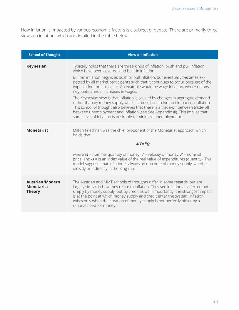
How inflation is impacted by various economic factors is a subject of debate. There are primarily three views on inflation, which are detailed in the table below.
School of Thought View on Inflation
Keynesian Typically holds that there are three kinds of inflation: push and pull inflation, which have been covered, and built-in inflation.
Built-in inflation begins as push or pull inflation, but eventually becomes ex-pected by all market participants such that it continues to occur because of the expectation for it to occur. An example would be wage inflation, where unions negotiate annual increases in wages.
The Keynesian view is that inflation is caused by changes in aggregate demand rather than by money supply which, at best, has an indirect impact on inflation. This school of thought also believes that there is a trade-off between trade-off between unemployment and inflation (see See Appendix III). This implies that some level of inflation is desirable to minimize unemployment.
Monetarist Milton Friedman was the chief proponent of the Monetarist approach which holds that:
where M = nominal quantity of money, V = velocity of money, P = nominal price, and Q = is an index value of the real value of expenditures (quantity). This model suggests that inflation is always an outcome of money supply, whether directly or indirectly in the long run.
Austrian/Modern Monetarist Theory
The Austrian and MMT schools of thoughts differ in some regards, but are largely similar in how they relate to inflation. They see inflation as affected not simply by money supply, but by credit as well. Importantly, the strongest impact is at the point at which money supply and credit enter the system. Inflation exists only when the creation of money supply is not perfectly offset by a rational need for money.
MV=PQ

Measuring Inflation | January 31, 2018
10 |
How is Inflation Measured Today?
During World War I, prices of a wide variety of goods, specifically market inputs like raw materials and fixed capital, increased rapidly. The CPI was devised to determine a consistent measure of how much money a consumer would need to buy a similar basket of basic goods, year-over-year. Since that time, the CPI has become a very popular measure of inflation. Each month, the BLS crunches the numbers on thousands of items purchased by consumers, ranging from toothpaste to automobiles.
While measuring prices at two discrete time periods and determining a price change is a simple concept, the conditions of the real-world present numerous challenges. Under the following constraints, the BLS aims to provide an accurate measure of consumer price increases:
› A lack of perfect and complete data › Fixed resources
› Constantly changing consumer preferences › Latent goods substitution
› Political oversight
The following section will provide an overview of how the CPI is calculated today.
Index Composition and Geographic Definitions
CPI-U is an index that measures inflation (CPI) for urban consumers. CPI-U, which includes food and energy costs, is the index that determines changes in social security, federal retirement benefits, individual income tax parameters, and Treasury Inflation-Protected Securities (TIPS)3. Today, CPI-U covers nearly 87% of the US population and a wide range of consumer goods. These goods can be summarized in a few overall expenditure categories. Figure 1 illustrates the current relevance weights by these expenditure categories. Note, however, that these weights are updated as new expenditure survey data becomes available, reflecting changes in consumer spending behavior.
Housing is by far the largest component, accounting for over 42% of the index. In particular, Shelter, which includes both owner-occupied and renter-occupied costs, represents more than a third of the index. This expenditure category has increased from just over 20% of the index in 1982 to nearly 34% today.
Figure 1. CPI Expenditure Category Relevance Weights (December 2016)
3. “Consumer Price Index: Frequently Asked Questions,” Bureau of Labor Statistics, U.S. Department of Labor https://www.bls.gov/cpi/questions-and-answers.htm
Housing; Shelter
Transportation Food & Beverages Education & Communication
Apparel, Recreation & Other House; Other Medical Care
33.7% 15.2% 14.7% 11.9% 9.0% 8.5% 7.0%

Unison Investment Management
11 |
It is important to note that there are a number of expenditures not included in the index. The following categories are excluded from CPI:
› Investments, such as stocks and bonds, business expenses, and life insurance
› Employer in-kind benefits, including employer-paid health insurance
› Taxes
› Government-provided and government-subsidized items
› Purchase of homes or other items that can be viewed as an investment
The BLS uses a defined set of geographies to create representative samples at the metro level. These also inform index contributions, or weights, for the national level indexes. The Census Bureau has divided the nation into nine major regions, which the BLS then sub-divides into Primary Sampling Units (PSUs). The PSU geographies are based on the definitions of Core-Based Statistical Areas (CBSAs), as defined by the U.S. office of Management and Budget (OMB). The BLS identifies PSUs as class A or B, depending on the size of the metro4. These are the geographic building blocks of all BLS inflation measurements. Figure 2 illustrates the distribution of class A and B PSUs across the nine regions.
PSUs are designed to achieve a sample that is well-distributed across the nation in terms of geography, population, and demographics. Further details on the geographic definitions process can be found in Appendix I.
Figure 2. The BLS Divisions for CPI (number of A and B PSUs within each region)
4. This approach – using nine major regions and only A or B areas – will begin to take effect in 2018. The current methodology only utilizes four regions and puts PSUs in three classes (A, B, and C areas).
Mountain (2A, 4B)
East North Central (2A, 8B)
Pacific (7A, 4B)
South Atlantic (5A, 12B)
Middle Atlantic (2A, 4B)
West North Central (2A, 4B)
West South Central (2A, 8B)
East South Central (6B)
New England (1A, 2B)

Measuring Inflation | January 31, 2018
12 |
Cost of Goods and Services (Excluding Housing)
Approximately 400 BLS field agents visit nearly 30,000 stores and collect prices on over 80,000 commodities and services each month. While the process of generating, maintaining, and collecting data for this sample of goods and services may be prone to error, it is vital for estimating the CPI.
Identifying ProductsThe CPI goods and services are mapped to a hierarchy with eight major groups, ranging from high-level categories (e.g., Apparel) down to specific entry-level items (ELIs: e.g., women’s dresses). The ELIs represent the units that are ultimately sampled. They are the lowest level category definition from which BLS field agents collect data at selected stores and outlets.
Examples of items and categories found in each of these levels is shown in the table below:
Figure 3. Hierarchy of Goods and Services Types (Count)
Major Groups (8)
Expenditure Classes (8)
Item Strata (211)
Entry-Level Items (Varies)
Major Groups Food and Beverages Apparel Housing
Expenditure Classes Cereals and Bakery Products
Women’s and Girls’ Apparel
Household Furnishings and Operations
Item Strata Bakery Products Women’s Apparel Furniture and Bedding
Entry-Level Items (ELI) Bread
Cakes, Cupcakes, and Cookies
Women’s Dresses
Women’s Suits and Separates
Bedroom Furniture
Other Furniture

Unison Investment Management
13 |
Item strata and ELIs essentially comprise the “consumer basket.” The items comprising this basket are updated over time as the Census Bureau conducts its Telephone Point of Purchase Survey (TPOPS)5, which is used to aggregate information on where consumers are shopping and what they are buying. Separately, the BLS collects expenditure data as a part of the Consumer Expenditure (CEX) survey6.
Ultimately, the BLS needs to obtain a list of stores to visit and entry-level items to price quote (i.e. ELI-store matches). Since it is infeasible for the BLS to sample every item from each of the item strata in every store across the nation, they use a model to find optimal combinations to sample from across the geographic regions and item strata7. This model is recalibrated twice a year. Figure 4 depicts the entire process, from data capturing through ELI-store matches.
Figure 4. How the BLS Determines ELI-Store Pairs
5. See Appendix I for more information.
6. This survey captures spending, income, and other demographic data of consumers in the US and is one of the more important data sources the BLS uses in the construction of CPI and other indexes.
7. Specifically, the BLS includes explicit budget constraints in the CPI estimation procedure. For a given budget, an optimal number of ELIs and regional stores are selected for sampling with the objective of minimizing CPI estimation variance. This optimization is performed over a combined 195 PSU-item strata grouping pairs (15 PSU groups and 13 item strata groups).
The Consumer Expenditure (CEX) Survey also captures
spending habits.
CEX survey and TPOPS data define the consumer basket.
This data updates the consumer basket.
TPOPS panel respondents report transactions quarterly.
Specific ELI-store matches that field agents will attempt to quote, such as women’s dresses + Macy’s
Reported expenditure data and outputs from the
item/store allocation are used to sample ELIs and
outlets.
The BLS uses a model to determine the number of items and stores per PSU to include in the pricing sample. This balances
price index variance and BLS organizational butdget. It is
updated semi-annually.
The Census Bureau conducts Telephone Point-of-Purchase
Survey (TPOPS) to collect expenditure data from roughly
200–400 people per PSU.

Measuring Inflation | January 31, 2018
14 |
The field agents work with store representatives to organize products into categories based on brand or packaging. Selection probabilities are assigned to each item group based on sales volume. A group is randomly selected and those items are stratified further into common groups. Probabilities are weighted by volume. This iterates until a single item is selected. One feature of this process is that two different items may be used to represent the same ELI in different outlets or index areas, since the random selection processes are independent.
Survey data and reported transactions serve as a feedback loop to update the consumer basket. This data and the BLS model inform which stores and items will be quoted and tracked in the index.
Data CollectionThe next step involves selecting the individual products that represent the ELIs and setting up a recurring process to collect price quotes over time. Yet another probability based, recursive sampling technique is required to determine the individual items. A large variety of goods can exist within a given ELI. For instance, there are diverse types women’s dresses that come in various colors, styles, and price points.
Figure 5. Process for Arriving at a Single Item to Quote for a Given ELI-Store Pair
This process is repeated, resulting in fewer items per
group in each iteration. A single item is eventually sampled.
Field agents start with a broad range of items in an ELI-Store combination.
The items are sorted into groups based on
brand and other simlarities.
A group of items is sampled, with
probabilities bassed on sales volume.
This process helps ensure a distribution of ELI item
sampling across stores and geographies.
p3p2p1
+

Unison Investment Management
15 |
The BLS notes that this helps reduce variance within an index component and correlations across regions. After this process is completed, the prices for the selected items are collected on a monthly or bi-monthly basis.
Field agents visit stores and record information on the products being tracked. Price, quantity, size, and sales tax are recorded. Product changes are also tracked and substitutions may occur due to:
› The release of a new, identical product of much better quality for the same or lower price.
› Trends in consumer purchases of a similar product that is offered at a lower price. These may be older or under a different brand.
› The increase in demand for a product that is quite different, yet offers the same consumer utility.
› Unexpected—and hard to detect—general changes in consumer preferences.
The BLS tackles these substitutions by: 1) assuming the products are essentially perfect substitutes; 2) attempting to use data from other products or regions to compute the price change; or 3) estimating the quality difference between one product and another. Manufacturing production data and various in-house hedonic models are used to measure the quality adjustments. Quality adjustments are often necessary, and several important CPI changes over the years were aimed at improving this process for specific items. These include changes in the quality adjustment calculations of Used Cars (1987), Apparel (1990), Personal Computers (1998), and TVs (1999). In addition, a geometric mean formula was introduced into the price relative estimation for some item indexes to better capture substitution effects (1999).
Adding It UpThe recorded price quotes, generated by the process described above, serve to calculate the relative price changes over time. Supplemental data is used to handle unique items, such as air and train fares, and special treatment is required for the pricing of various categories, including medical care, health insurance, and vehicles. In addition, other adjustments are necessary to account for discounts, sales, and rebates8.
Price relatives for most CPI items are defined as the weighted geometric average of the item’s current price divided by its previous price (the item’s price ratio). These price relatives are calculated for each item-area combination, taking into account different prices in different areas, with each price ratio scaled by the item’s expenditure weight. Each item-area price relative can then be used to move CPI “elementary” indexes from month-to-month or year-to-year. See Appendix I for the relevant equations.
8. For a full list and description of these special treatment items, refer to the BLS Handbook of Methods, Chapter 17, pages 22–28.

Measuring Inflation | January 31, 2018
16 |
Cost of Housing
Housing is by far the largest component of the CPI. Shelter alone accounts for over a third of the overall index. The housing-related expenses explicitly covered include:
› Cost of shelter (rent and owner-occupied)
› Energy and utilities
› Furnishings, appliances, and other operations
› Miscellaneous supplies, such as tools and cleaning products
Many housing related items can be treated with the standard procedure. However, the cost of shelter, particularly owner-occupied housing and rent, as measured by Owners’ Equivalent Rent of Primary Residences (OER) and Rent of Primary Residences (Rent), respectively, present unique challenges. This section focuses on how the BLS measures the cost of owner-occupied and rental housing services.
The BLS implements a three-step sampling procedure before rolling the estimates of the OER into the CPI, estimating:
1. the OER and rent percentage contribution to total spending (survey based);
2. the geographic sampling rates (regression based);
3. the price changes over time (market based).
Percentage of Total SpendingFirst, the BLS determines what percentage of a family’s expenditures is allocated to rent. This percentage is estimated by asking homeowners the following question:
“If someone were to rent your home today, how much do you think if would rent for monthly, unfurnished and without utilities?”
An analogous question is posed to renters:
“What is the rental charge to your [household] for this unit, including any extra charges for garage and parking facilities? Do not include direct payments by local, state, or federal agencies. What period of time does this cover?”
When rolled into the final CPI, the weights of these item categories—namely OER and Rent—are estimated based on the responses to these questions. A considerable risk of sampling bias and observation noise is introduced by polling, rather than observing market rents. It assumes that homeowners can generate strong signals of the latent rents they are implicitly paying to live in their homes.
An alternative calculation could take a regionwide median (or average) market rent divided by average (or median) total spending. However, in an economy with relatively poorer renters and wealthier homeowners, observable markets rents might exhibit a downward bias. This framework would consistently underrepresent housing expenses as a function of total spending in regions with high inequality of wealth and/or income.
9. Census Block Groups are Census defined geographic identifiers, between Census Tracts and Census Blocks in size. Each Block Group typically has a population of 600-3,000 people.

Unison Investment Management
17 |
The problem of estimating the rent component of spending each year is far from trivial, and there is a good reason to sample these percentage contributions to overall spending on an individual-by-individual basis.
Geographic Sampling RateThe current methodology for housing unit sample generation was first used in 1998 to create a 25,000-unit housing sample using 1990 decennial Census data. A recycle process initiated in 2012 has replaced and expanded most of this sample by leveraging data from the 2000 decennial Census. The units are spread across the all PSUs in distinct segments made up of one or more Census Block Groups9. Each Block Group in the larger and smaller PSUs contained, respectively, at least 50 and 30 housing units. Each segment was designed to have an average of 150 units. A subset of the more than 200,000 Census Block Groups were sampled with a probability proportional to the estimated Total Cost (TC) of housing in each segment. To ensure this sample was geographically representative on the national level, as well as on that of the PSU, each PSU was split into six separate sections that each contained roughly one-sixth of the PSU housing stock. The segments within each section were then rank ordered by county and average rent level before being sampled. An example of this outcome is shown in Figure 6 for the Las Vegas metro area.
10. This is strictly for illustration purposes and does not depict actual BLS sampling results for the Las Vegas area.
Figure 6. Example of the Block Group Sampling Process10.
› The PSU is split into six sections, each containing approximately the same amount of housing stock.
› Block Groups are sampled (shown in blue).
› Properties in these areas will be screened for sample eligibility.

Measuring Inflation | January 31, 2018
18 |
TC was the primary driver of the sampling process. It is defined as the sum of average rent and implicit rent, scaled by the number of rental units and owner-occupied units, respectively. Formal definitions of TC, imputed rents, and the selection probabilities can be found in Appendix I.
Once the segments are selected, field agents travel to the neighborhoods and “tag” the housing units by creating a list of all addresses. Until recently, field agents had to physically add all addresses to the database manually and had no information regarding the occupancy status of the home. Now, the BLS uses purchased address lists to increase the efficiency of selecting eligible properties and reduce the burden on its resources. Once the list is created, a subset of these addresses is generated by yet another sampling algorithm to determine which units would be approached by the field agents to screen for eligibility.
If the home is eligible, the field agent would begin collecting information from the homeowner, tenant, or landlord. In-scope properties11 must:
› Be renter-occupied
› Be the primary residence of the occupant
› Not have tenants that are relatives of the landlord
› Not be institutional, public, or assisted-living housing
In-scope units continue to the “initiation” phase, at which point information is gathered, including the amount of rent paid and any housing services, subsidies, or extra charges (e.g., parking) associated with rent. The BLS aims to have at least five in-scope units in each segment at all times. This minimum has not always been met for all segments.
11. Note that rent-controlled units are eligible for the sample. The index calculation excludes these units from having an impact on the OER (by applying an individual unit owner-occupied weight of 0), but these units’ price movements, or lack thereof, do affect the Rent index.
Figure 7. Housing Sample Data Collection Process
Field agents tag all housing units in the segment neighborhoods. Today, they use purchased address lists to assist them in this task.
A sampling algorithm selects housing units for field agents to check eligibility.
Eligible units must meet specific conditions, such as being renter-occupied, and not institutional, public, or assisted-living housing.
The previous national sample was initially ~25,000 units. It was enhanced over time with new construction and the other units to nearly 35,000. The national sample is currently being refreshed.
Eligible sample units are split into six panels. Only one group is surveyed each month, with data collected for each on a semi-annual basis.
JanJuly
FebAug
MarSept
AprOct
MayNov
JuneDec

Unison Investment Management
19 |
Because the BLS finds that rents are not as volatile as other consumer goods, they do not collect data on all housing units each month. Instead, segments within a PSU are split into six panels. In any given month, only one panel is surveyed, such that data is recorded for each panel twice a year (every six months). This also implies that each month the national OER and Rent indexes are estimated with data from only one-sixth of the total housing sample, or approximately 6,000 units. For comparison, as of 2016, there were roughly 42.2 million renter-occupied and 74.7 million owner-occupied units in the US12.
At every six-month visit, the field agent confirms the unit is still eligible and can remain in-scope. They also document the rent that is being paid, any changes to services, and any interior alterations made to the home, such as increased square footage or bed/bath count. These changes in service and quality adjustments affect the final value of the rent used in the index construction.
Price Change over TimeThe actual paid rent values disclosed by the surveyed tenants are first normalized to convert all values to monthly rents, and used to estimate the change in price levels over time. The BLS computes Economic Rents by accounting for age and changes in quality or services from one measurement period to the next. The age bias and other adjustment types are summarized in the table below. Economic Rents and the weights associated with the units are the building blocks for the Rent price relatives.
Adjustment Description
Age Bias The BLS accounts for depreciation due to age by adjusting the prior period’s ER downward. A hedonic regression model was used to estimate the size of this bias. The results show that the age bias slightly varies across PSUs, but the annual impact is approximately 0.3% for both Rent and OER indexes.
Structural Changes
Includes remodeling done to unit, such as added square footage, additional bedrooms or bathrooms, or new A/C units. The same hedonic regression model estimates these adjustment factors.
Utilities Changes Accounts for changes in energy, water, and sewer provided services.
Facility Changes Accounts for changes in parking, A/C, or other building facilities.
Analyst Discretion Manual adjustments made by field agent if it is determined an adjustment is not captured by the other categories.
Pure Rents are used for the OER price relatives and are identical to Economic Rents, save one key distinction. Since homeowners pay their own utilities, these costs are excluded from Pure Rents. Rents and weights are then used to compute the OER price relatives.
12. Census Bureau American Community Survey (ACS) 2015 5-year estimates.

Measuring Inflation | January 31, 2018
20 |
With the necessary ingredients for each segment—average and imputed rents, distribution of rental and owner-occupied units, and Economic and Pure Rents—the OER and Rent price relatives and indexes can be generated. Rental and owner-occupied weights for a segment are simply the geographic weight of that segment scaled by the number of rental and owner-occupied units, respectively, in the segment. In addition, the owner-occupied weight is influenced by the ratio of imputed to average rents. The higher the segment’s imputed rent, relative to the average rent, the larger the weight. The six-month Rent (OER) price relative is defined as the weighted sum of this measurement period’s Economic Rent (Pure Rent) relative to that of the previous measurement period. These are transformed into one-month price relatives13 to match those of other goods and services. Each one-month area price relative is then used to move CPI elementary Rent and OER indexes, as with other item-area combinations.
Higher Level Index Aggregation
Once all 8,000+ basic item-area indexes are computed, they are aggregated using the values of the elementary indexes and aggregated expenditure weights.
Estimated prices and quantities for item-area combinations (e.g., apparel cost in a neighborhood of San Francisco) determine the aggregate (i.e., relevance) weights representing consumer preferences. Previously, these estimates were refreshed on a decennial basis, but the BLS now rebases them on a more frequent schedule—once every two years—using CEX survey data. Weights are now computed using item-area price changes. The implied relevance weights are free to change between rebase periods14.
The Laspeyres price formula is used in the aggregation formula. Intuitively, the formula estimates the price change of a constant basket of goods. Mechanically, the index change is calculated as a weighted average change in the sub-indexes. The weights of each of the sub-indexes are only updated at the beginning of a new rebase period. This can be generally defined as follows:
Where:
Finally, the resulting index values are used to compute the month-on-month or year-on-year CPI changes.
Inflation and Its Impact on Real Estate | October 31, 2017
Intellectual property of Unison Investment Management Proprietary and confidential Page 19 of 56
With the necessary ingredients for each segment—average and imputed rents, distribution of rental and owner-occupied units, and Economic and Pure Rents—the OER and Rent price relatives and indexes can be generated. Rental and owner-occupied weights for a segment are simply the geographic weight of that segment scaled by the number of rental and owner-occupied units, respectively, in the segment. In addition, the owner-occupied weight is influenced by the ratio of imputed to average rents. The higher the segment’s imputed rent, relative to the average rent, the larger the weight. The six-month Rent (OER) price relative is defined as the weighted sum of this measurement period’s Economic Rent (Pure Rent) relative to that of the previous measurement period. These are transformed into one-month price relatives13 to match those of other goods and services. Each one-month area price relative is then used to move CPI elementary Rent and OER indexes, as with other item-area combinations.
Higher Level Index Aggregation
Once all 8,000+ basic item-area indexes are computed, they are aggregated using the values of the elementary indexes and aggregated expenditure weights. Estimated prices and quantities for item-area combinations (e.g., apparel cost in a neighborhood of San Francisco) determine the aggregate (i.e., relevance) weights representing consumer preferences. Previously, these estimates were refreshed on a decennial basis, but the BLS now rebases them on a more frequent schedule—once every two years—using CEX survey data. Weights are now computed using item-area price changes. The implied relevance weights are free to change between rebase periods14. The Laspeyres price formula is used in the aggregation formula. Intuitively, the formula estimates the price change of a constant basket of goods. Mechanically, the index change is calculated as a weighted average change in the sub-indexes. The weights of each of the sub-indexes are only updated at the beginning of a new rebase period. This can be generally defined as follows: Equation 1
𝐼𝐼𝐼𝐼𝑋𝑋-,/0,1,2 = 𝐼𝐼𝐼𝐼𝑋𝑋-,3
0,1,2 ×∑ 𝐴𝐴𝑊𝑊8
9,:,2 × 𝐼𝐼𝐼𝐼𝑋𝑋/9,:∈(0,1)
∑ 𝐴𝐴𝑊𝑊89,:,2 × 𝐼𝐼𝐼𝐼𝑋𝑋39,:∈(0,1)
Where:
› 𝐼𝐼, 𝐴𝐴 = the set of elementary items. This is all elementary items for CPI-U. › 𝐴𝐴 = the set of elementary areas. This is all elementary areas (US city average) for CPI-U. › 𝑝𝑝 = population › 𝑖𝑖, 𝑎𝑎 = elementary item and area, respectively
13 This also has the effect of smoothing the series. 14 To reduce expenditure weight variance for the elementary item-area combinations, the BLS employs some smoothing techniques when computing the aggregation weights. For more details, see Exhibit 3 of the BLS Handbook of Methods, Chapter 17.
Inflation and Its Impact on Real Estate | October 31, 2017
Intellectual property of Unison Investment Management Proprietary and confidential Page 20 of 56
› 𝑏𝑏 = aggregated index base period. This is 1982–84 for CPI-U. › 𝑣𝑣 = year/month just prior to expenditure weights rebase period 𝛽𝛽 › 𝐴𝐴𝑊𝑊8 = aggregate weight from rebase period 𝛽𝛽 › 𝐼𝐼𝐼𝐼𝑋𝑋/ = the lower-level index price change from the index’s base year to month 𝑡𝑡 › 𝐼𝐼𝐼𝐼𝑋𝑋3 = the lower-level index price change from the index’s base year to rebase month 𝑣𝑣
Finally, the resulting index values are used to compute the month-on-month or year-on-year CPI changes.
Inflation and Its Impact on Real Estate | October 31, 2017
Intellectual property of Unison Investment Management Proprietary and confidential Page 19 of 56
With the necessary ingredients for each segment—average and imputed rents, distribution of rental and owner-occupied units, and Economic and Pure Rents—the OER and Rent price relatives and indexes can be generated. Rental and owner-occupied weights for a segment are simply the geographic weight of that segment scaled by the number of rental and owner-occupied units, respectively, in the segment. In addition, the owner-occupied weight is influenced by the ratio of imputed to average rents. The higher the segment’s imputed rent, relative to the average rent, the larger the weight. The six-month Rent (OER) price relative is defined as the weighted sum of this measurement period’s Economic Rent (Pure Rent) relative to that of the previous measurement period. These are transformed into one-month price relatives13 to match those of other goods and services. Each one-month area price relative is then used to move CPI elementary Rent and OER indexes, as with other item-area combinations.
Higher Level Index Aggregation
Once all 8,000+ basic item-area indexes are computed, they are aggregated using the values of the elementary indexes and aggregated expenditure weights. Estimated prices and quantities for item-area combinations (e.g., apparel cost in a neighborhood of San Francisco) determine the aggregate (i.e., relevance) weights representing consumer preferences. Previously, these estimates were refreshed on a decennial basis, but the BLS now rebases them on a more frequent schedule—once every two years—using CEX survey data. Weights are now computed using item-area price changes. The implied relevance weights are free to change between rebase periods14. The Laspeyres price formula is used in the aggregation formula. Intuitively, the formula estimates the price change of a constant basket of goods. Mechanically, the index change is calculated as a weighted average change in the sub-indexes. The weights of each of the sub-indexes are only updated at the beginning of a new rebase period. This can be generally defined as follows: Equation 1
𝐼𝐼𝐼𝐼𝑋𝑋-,/0,1,2 = 𝐼𝐼𝐼𝐼𝑋𝑋-,3
0,1,2 ×∑ 𝐴𝐴𝑊𝑊8
9,:,2 × 𝐼𝐼𝐼𝐼𝑋𝑋/9,:∈(0,1)
∑ 𝐴𝐴𝑊𝑊89,:,2 × 𝐼𝐼𝐼𝐼𝑋𝑋39,:∈(0,1)
Where:
› 𝐼𝐼, 𝐴𝐴 = the set of elementary items. This is all elementary items for CPI-U. › 𝐴𝐴 = the set of elementary areas. This is all elementary areas (US city average) for CPI-U. › 𝑝𝑝 = population › 𝑖𝑖, 𝑎𝑎 = elementary item and area, respectively
13 This also has the effect of smoothing the series. 14 To reduce expenditure weight variance for the elementary item-area combinations, the BLS employs some smoothing techniques when computing the aggregation weights. For more details, see Exhibit 3 of the BLS Handbook of Methods, Chapter 17.
› › › › › › › › ›
13. This also has the effect of smoothing the series.
14. To reduce expenditure weight variance for the elementary item-area combinations, the BLS employs some smoothing techniques when computing the aggregation weights. For more details, see Exhibit 3 of the BLS Handbook of Methods, Chapter 17.


Measuring Inflation | January 31, 2018
22 |
A Short History of Housing and Inflation
The most relevant CPI component to our analysis has also arguably been the most scrutinized one over the last 60 years. Housing comprises over 42% of the CPI-U All Items index. Shelter alone accounts for nearly one-third, with the important indexes of Rent of Primary Residences (Rent) and Owners’ Equivalent Rent of Primary Residences (OER) accounting for 7.9% and 24.6%, respectively15. Computing the change in the cost of shelter is by no means trivial, and, given the fact these components are such a large portion of CPI, these two indexes have drawn much attention over the years from researchers, politicians, organized labor groups, and investors. This section will track the evolution of the CPI methodology used to measure the cost of rental and owner-occupied housing, highlighting important changes and sources of weakness.
Before the Benchmark Years (1950–1983)
In the early 1950s, the BLS began using a Cost of Purchase (Asset Price) method to determine the cost of owner-occupied housing. This approach considers the purchase of a home as the purchase of a non-durable good, with the full cost of the good accounted for in the period the home is purchased. This definition includes goods purchased on credit, such as a home using a mortgage. To measure the month-to-month change in the cost of housing, the BLS assessed five expense factors of homeownership:
› Property Taxes › Insurance › Maintenance and Repairs
› House Prices › Mortgage Interest Costs
Weights for these five factors were derived from past CEX surveys. The first three general recurring expenses were gathered through standard surveying procedures. The last two—house prices and mortgage interest costs—were influenced by recent home sales and mortgage rates. Despite being a reasonable approach to capture the cost of homeownership at a given point in time, criticism grew through the next two decades, leading to substantial efforts by the BLS to research and implement alternative methods.
The 1961 Stigler Report16, commissioned by the Bureau of the Budget, formally documented deficiencies in the CPI at the time. The report put forth a fundamental concern with respect to how the cost of housing was accounted for in the index, asserting that the Asset Price methodology failed to properly isolate the flow of services consumers yield from housing. Specifically, a home can be viewed as both an asset that can be purchased and resold later (realizing a capital gain or loss) and as a durable good through which an owner consumes housing. Unlike a meal at a restaurant, these services are not consumed immediately, but are enjoyed over an extended period. The CPI is theoretically intended to reflect changes in consumption; thus, investments, such as stocks and bonds, are intentionally excluded. The critical question here is to what extent is a home an investment and to what extent is it an item of consumption.
15. “Relative importance of components in the Consumer Price Indexes: US city average, December 2016.” Page 2. https://www.bls.gov/cpi/relative-importance-2016.pdf.
16. George Stigler, ed., “’The Price Statistics of the Federal Government,” Report to the Office of Statistical Standards, Bureau of the Budget. (New York: National Bureau of Economic Research, 1961)

Unison Investment Management
23 |
The authors of the Stigler Report were concerned about the faultiness of this method of calculating CPI and urged the BLS to move to an alternative, endorsing a rental equivalence method. By the late 1970s, much internal research and deliberation had occurred on rental equivalence and user cost methods17, but no consensus had been arrived at. In addition to internal division, the BLS received pressure from various political agencies, task forces, and labor union representatives, including those from the American Federation of Labor and Congress of Industrial Organizations (AFL-CIO). The use of CPI indexation grew, leading more parties with vested interests to join the shelter methodology debate. The following developments transpired from 1975–81 and cemented CPI’s status as a political tool:
› Starting in 1975 Social Security benefits, including disability insurance, was pegged to CPI.
› Nearly one out of every three dollars the federal government spent was directly linked to CPI by 1981. At that time, introducing new indexed expenditures could have impacted over half of the federal budget.
› Income tax brackets became tied to the index in 1981 through the Economic Recovery Tax Act.
› Numerous wage contracts and collective bargaining agreements were indexed to CPI.
At the time, changes in the CPI had a substantial effect on government payments, with a 1% rise in the CPI corresponding to an approximate $2B increase in federal outlays ($5.25B in 2017, adjusted for the change in the value of gold18). It was no longer a theory vs. practice consideration, but one of significant political and budgetary importance. It was in the government’s best interest to keep inflation low and volatility down.
Large, sharp increases to outlays due to indexation would result in ripple effects, not the least of which involved the risk of deficit financing. On the other side of the equation, labor unions strongly opposed any changes to the shelter methodology. Increases in CPI led to wage contract escalations for their constituents. These groups were clearly aware of the prospect of unfavorable results from altering a component that made up a quarter of the overall index and was undoubtedly the driving force in the late 1970s–early 1980s sharp rise in CPI as house prices and mortgage rates rose rapidly. As this spike in inflation developed, calls for changes increased from government bodies, including the Council of Economic Advisors and the Congressional Budget Office.
The market dynamics of the time exposed some of the shortcomings of the Asset Price method. Critics pointed to five major drawbacks:
1. Investment-like features: Accounting for net sales of homes in each period implicitly includes capital gains accrued on these sold homes. Proponents of alternative cost measures of owner-occupied housing insisted that the Asset Price method included both consumption and investment aspects of housing, which is counter to CPI’s intended design of excluding investments.
17. See Appendix II for details on the user cost method.
18. Authors’ Note: The intention of this paper is to provide insight into how CPI is calculated; specifically, the housing component of CPI. The tabulation and methodology of inflation is being questioned within this paper, and we determined that another measure

Measuring Inflation | January 31, 2018
24 |
2. House Price Data: The BLS utilized FHA (Federal Housing Administration) home sales data for monthly estimates of home prices and sales. Homes purchased above the FHA qualifying maximum loan amount were excluded, resulting in a downward bias. In addition, as more mortgage products were being introduced to consumers, FHA loans were becoming a smaller portion of the market. Relying solely on the FHA data gave the BLS a shrinking perspective on monthly home sales.
3. Housing Expenditure Weights: The 1981 expenditure weights for the five housing factors were derived from the 1972–73 CEX survey. This survey was not only nearly ten years old at this time, it also offered a questionable home purchase expenditure weight. Only 3% of the survey population purchased a house during the survey period. Further, only the costs associated with home and mortgage purchase contributed to the weights. Those households that already owned a home (and were making mortgage payments) were not considered. In other words, 97% of the survey population had no contribution to the weightings of two of the five homeownership expense factors.
4. Current Mortgage Rate: The CPI did not assume that all homeowners (re)purchase their homes each month; they only assessed the index based on homes purchased in the given month at the prevailing mortgage rate. Homeowners that had purchased a home in prior periods, possibly at a different mortgage rate, were not considered, even though they were presumably making monthly mortgage payments.
5. Volatility: Since the owner-occupied cost index was a large portion of the overall CPI and was constructed using current mortgage rates, changes in the index were strongly tied to mortgage rate movements. Sharp changes in mortgage rates and house prices led to higher CPI volatility, variation that is generally deemed undesirable.
The BLS attempted to stand their ground through the criticism. The then BLS Commissioner, Janet Norwood, stressed that the root of these concerns was political and best resolved in that manner. She put it this way when testifying before Congress:
“Some people would like an index that doesn’t go up so much, and other people would like an index that goes up more. And when they don’t have that which they want, they feel there must be something wrong with the indicator itself.”19
The Bureau continued to research alternatives and began publishing experimental CPI indexes. These indexes showed what CPI would have been were different homeownership cost approaches used, including OER and user cost measures. The user cost method suffered from poor house price data and led to an unusable index, as home transactions were projected to stall when mortgage rates rose to extreme levels.
The experimental index leveraging the OER method had the lowest average annual inflation and resulted in a less volatile series than the official CPI. In addition, it was nearly 2% lower than the official index by the early 1980s. These findings, coupled with continual pressure to implement change, led the BLS to replace the Asset Price process with an OER methodology. This major revision was made effective January 1983 and coincided with the current benchmark years of 1982–84 (when prices were indexed to 100).
19. Darren Rippey, “The first hundred years of the Consumer Price Index: a methodological and political history,” Monthly Labor Review, Bureau of Labor Statistics, 2014, https://www.bls.gov/opub/mlr/2014/article/the-first-hundred-years-of-the-consumer-price-index.htm
Unison Investment Management
25 |
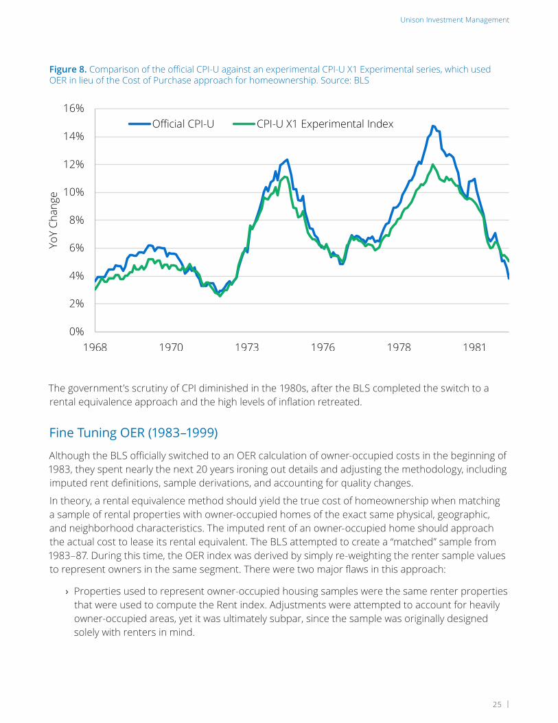
Figure 8. Comparison of the official CPI-U against an experimental CPI-U X1 Experimental series, which used OER in lieu of the Cost of Purchase approach for homeownership. Source: BLS
The government’s scrutiny of CPI diminished in the 1980s, after the BLS completed the switch to a rental equivalence approach and the high levels of inflation retreated.
Fine Tuning OER (1983–1999)
Although the BLS officially switched to an OER calculation of owner-occupied costs in the beginning of 1983, they spent nearly the next 20 years ironing out details and adjusting the methodology, including imputed rent definitions, sample derivations, and accounting for quality changes.
In theory, a rental equivalence method should yield the true cost of homeownership when matching a sample of rental properties with owner-occupied homes of the exact same physical, geographic, and neighborhood characteristics. The imputed rent of an owner-occupied home should approach the actual cost to lease its rental equivalent. The BLS attempted to create a “matched” sample from 1983–87. During this time, the OER index was derived by simply re-weighting the renter sample values to represent owners in the same segment. There were two major flaws in this approach:
› Properties used to represent owner-occupied housing samples were the same renter properties that were used to compute the Rent index. Adjustments were attempted to account for heavily owner-occupied areas, yet it was ultimately subpar, since the sample was originally designed solely with renters in mind.
Inflation and Its Impact on Real Estate | October 31, 2017
Intellectual property of Unison Investment Management Proprietary and confidential Page 25 of 56
Figure 8. Comparison of the official CPI-U against an experimental CPI-U X1 Experimental series, which used OER in lieu of the Cost of Purchase approach for homeownership. Source: BLS
Fine Tuning OER (1983–1999)
Although the BLS officially switched to an OER calculation of owner-occupied costs in the beginning of 1983, they spent nearly the next 20 years ironing out details and adjusting the methodology, including imputed rent definitions, sample derivations, and accounting for quality changes. In theory, a rental equivalence method should yield the true cost of homeownership when matching a sample of rental properties with owner-occupied homes of the exact same physical, geographic, and neighborhood characteristics. The imputed rent of an owner-occupied home should approach the actual cost to lease its rental equivalent. The BLS attempted to create a “matched” sample from 1983–87. During this time, the OER index was derived by simply re-weighting the renter sample values to represent owners in the same segment. There were two major flaws in this approach:
› Properties used to represent owner-occupied housing samples were the same renter properties that were used to compute the Rent index. Adjustments were attempted to account for heavily owner-occupied areas, yet it was ultimately subpar, since the sample was originally designed solely with renters in mind.
0%
2%
4%
6%
8%
10%
12%
14%
16%
1968 1970 1973 1976 1978 1981
YoY
Chan
ge
Official CPI-U CPI-U X1 Experimental Index

Measuring Inflation | January 31, 2018
26 |
› The same rent values were used for both Rent and OER price differentials. These Economic Rents included ancillary services, such as utilities, and ideally would not be used for OER.
January 1987 marked the first changes made to the OER methodology with the introduction of new rent values excluding utilities (Pure Rents) for OER and the use of a new 20,000 owner-occupied unit sample. In addition, owner-occupied weights for the geographic segments were updated with 1980 Census values. The OER index calculation now worked as follows:
› Each homeowner was asked to estimate the implicit rental value of their home. This served as the base value for the individual unit.
› An algorithm was used to match renter units to individual owner-occupied units, based on structural features, age, the number of units, and location characteristics.
› Changes in the Pure Rent of these matched renters were used to move the implicit rent of the owner, initially set by the estimate from the homeowner. These changes were subsequently weighted by the owner weights and used to adjust the OER index.
This process remained in place for the next twelve years. During that time, several other changes were made, including:
› Quality adjustments to individual units based on a hedonic regression model, which specifically focused on the effects of age. A version of this was first implemented in 1988. The regression model was updated in 1999, and currently includes 28 variables. Results have led to an annual age adjustment in the Rent and OER indexes of roughly 0.3%. Other structural and service change adjustments (e.g., for number of beds/baths, the inclusion of gas or parking, etc.) are also derived from this model.
› Modifications made to the matching algorithm and formulas used to move the implicit rents.
› Introduction of a six-month chained price differential from a one-month composite.
Matching rental samples with owner-occupied units was a valiant attempt at producing a theoretically sound OER index; however, the resources and time required to source and maintain this method became overwhelming for the BLS. Finding matched renter-owner sets proved to be quite challenging. Relaxing property characteristic constraints in the algorithm resulted in poor matches. The matching method was also resource intensive. They discontinued the process and reverted to the re-weighting method in 1999. Eliminating the owner sample resulted in less work for BLS field agents and easier data maintenance. The sample was refreshed using data from the 1990 Census, replacing the housing units and weights derived over 15 years prior.
With the reversion back to the re-weighting process, the BLS also decided to use changes in Pure Rents, rather than implicit rents, as the basis for the OER price differential. This was an important, yet subtle, change. Previously, homeowners in the owner-occupied sample were asked to offer an implicit rent for their home. This value was used as the base rent, and changes in the Pure Rents of the rental units were used to adjust this base value. The implicit rent collection was discontinued with the changes in 1999. Changes in Pure Rents were no longer moving base values provided by owner-occupied residents in the sample.

Unison Investment Management
27 |
This 20-year period highlighted some shortcomings of the change to an OER method. Aside from the attempt at a theoretically sound sample for a rental equivalence measure, which was abandoned in the late 1990s, other potential drawbacks of the methodology are noteworthy:
› Sample Deficiencies: The lack of sample refresh is woefully apparent. The first sample in the 1983–87 period attempted to augment a full renter sample with more renter samples in owner-occupied concentrated areas to improve the weights. The 1987 revision yielded a full refresh using 1980 Census data. At that point, the survey data was seven years old. All units (rental and owner-occupied) in the sample were built before 1980. This sample would persist until the refresh in 1999. It follows, therefore, that the vast majority of the housing sample units in the years leading up to the refresh were at least 20 years old.
› Implicit Rent Weights: Housing unit sampling is the way the BLS estimated the total housing costs, which is simply the sum of the estimated rental and owner costs in a given area. An important variable in the Total Cost definition is an estimate of average owners’ equivalent (imputed) rent. For the better part of 15 years, the BLS used a nonlinear regression method, fitted to 1990 Census Block data. Average rent and average estimated owner value were used as variables to estimate average imputed rent. This estimation procedure changed drastically in the 2000s. The model specification was changed to a linear regression, more regressors were added, and the geographic reach of the underlying data was expanded20. Such a dramatic alteration in the estimation model indicates insurmountable challenges in estimating the implicit rent.
20. See equation A5 in Appendix I.
Figure 9. Owners’ Equivalent Rent (OER) series stayed in a tight range while national house prices, as measured by the National Case-Shiller index (National C-S), went through a full cycle (1984–1999).
Inflation and Its Impact on Real Estate | October 31, 2017
Intellectual property of Unison Investment Management Proprietary and confidential Page 27 of 56
Relaxing property characteristic constraints in the algorithm resulted in poor matches. The matching method was also resource intensive. They discontinued the process and reverted to the re-weighting method in 1999. Eliminating the owner sample resulted in less work for BLS field agents and easier data maintenance. The sample was refreshed using data from the 1990 Census, replacing the housing units and weights derived over 15 years prior. With the reversion back to the re-weighting process, the BLS also decided to use changes in Pure Rents, rather than implicit rents, as the basis for the OER price differential. This was an important, yet subtle, change. Previously, homeowners in the owner-occupied sample were asked to offer an implicit rent for their home. This value was used as the base rent, and changes in the Pure Rents of the rental units were used to adjust this base value. The implicit rent collection was discontinued with the changes in 1999. Changes in Pure Rents were no longer moving base values provided by owner-occupied residents in the sample. Figure 9. Owners’ Equivalent Rent (OER) series stayed in a tight range while national house prices, as measured by the National Case-Shiller index (National C-S), went through a full cycle (1984–1999).
This 20-year period highlighted some shortcomings of the change to an OER method. Aside from the attempt at a theoretically sound sample for a rental equivalence measure, which was abandoned in the late 1990s, other potential drawbacks of the methodology are noteworthy:
-4%
-2%
0%
2%
4%
6%
8%
10%
1984 1986 1989 1992 1994 1997
YoY
Chan
ge
National C-S CPI-U OER

Measuring Inflation | January 31, 2018
28 |
Since this estimation is a key input in segment sampling and the eventual sample weighting in the construction of the index, there are adverse downstream consequences if it is not estimated accurately.
› More Political Meddling: In 1995, then Federal Reserve Chairman Alan Greenspan spoke in front of the House and Senate Budget Committees and claimed that CPI overestimated annual inflation by 0.5 to 1.5%. The Committees were concerned about deficit reductions, and Mr. Greenspan offered a helpful suggestion by saying that Congress could save up to $5B over the next five years if more changes were made to the way CPI was calculated. Although former Chairman Greenspan did not specifically call out housing costs in his testimony, this event is another illustration of political intrusion over the years. Producing the best possible cost of living index for the US citizens and markets has clearly not been a priority for the US government. It has had the motivation of keeping inflation, and indexed government costs, artificially low.
Through the Housing Boom and Bust and Beyond (1999–Present)
Few changes have been made to the OER computations in the past 15–20 years; however, important sampling technique adjustments were made in 2012 and are in use today. Comparing the current state with previous sample characteristics illustrates not only the challenges the BLS faces in sample construction, but also the consequential impact the issues with sample have on the practicality of a true OER. Sample details and attempted remedies before the 2012 refresh include:
› Size: The 1999 refresh, using 1990 Census data, fell incredibly short of its 50,000-unit goal. The result was a sample of only about 25,000 eligible properties. This was augmented to roughly 34,000 by adding recently constructed units and older eligible units. Yet this was still only two-thirds the size of the target sample. When you consider the paneling structure of the data collection, only one-sixth of these 25,000–34,000 contributed to the housing index in a given month. In other words, the monthly Rent and OER indexes for a nation with about 100mm properties was estimated with a sample of ~6,000 units.
› Composition: The BLS has designed the sampling procedure to generate a set of rentals and owner-occupied units that are geographically distributed in proportion to total housing cost. In addition, the distribution of rentals vs. owner-occupied in each region is intended to be representative of the number of rentals and owner-occupied units in that geography. The actual composition of the sample used throughout the 2000s had a deficiency in the low-percent rent segments. By the end of 2004, those segments with 0-10% rental units represented only 5% of the total sample. In other words, neighborhoods that had the highest concentration of owner-occupied dwellings had a low contribution to the indexes. Moreover, units in areas with higher concentration of owner-occupied homes (70–100%) tended to fall out of the sample (i.e., become ineligible) more frequently. Only approximately 60% of the sample of homes in these buckets were still eligible six years after being added to the sample. Properties currently being rented in highly concentrated owner-occupied regions have a higher probability of transitioning from a rental to an owner-occupied dwelling. Attribution issues were very prominent in these categories, which comprised nearly 40% of the total housing sample.

Unison Investment Management
29 |
› Age: A glaring issue with the sample construction was the use of lagged data to compute the segment rental and owner weights and the lack of recently constructed units in the sample. The 1980 Census was used in the sample construction of 1987, which lasted until 1999. The refresh in 1999 leveraged the 1990 Census and was not fully recycled until after 2012. The insight here is that by the end of the sample’s life, the weightings used in the price differentials were derived using data collected nearly 20 years before. Housing and demographic changes are slow moving tides, but much can transpire over two decades, particularly at the neighborhood or census block level. As an example, Las Vegas’ population increased 226% between the 1990 and 2010 censuses21. Furthermore, the weighted-average age of the units themselves would be at least 20 years old. All units included in the sample at the point of refresh were to be built prior to the decennial census used. Very few newly constructed units were added to augment the sample over time. The BLS does account for quality changes associated with age and structure changes at the unit level, but it is an imperfect process and the sample construction fails to account for changing consumer preferences and costs associated with them. New construction styles and quality fail to make it into the indexes while units of outdated styles and features persist.
Housing refreshes (weights and units) were updated once every ten years, following the update frequency of other CPI categories, including consumer preferences, items, and stores; geographic definitions; and collection and estimation methods. In 2002, the update frequency was increased for several of these categories, yet changes to housing did not begin until 2010. The sample improvements were slated to occur in multiple stages. The first two stages cycled in units from the 2000 Census to replace those from the 1990 Census. This process took six years, and May 2016 was the first month in which the entire sample was drawn from the 2000 Census. This means the “new” data is already sixteen years old.
The final planned stage is to implement a more continuous replacement process that will leverage the 2010 Census and more frequent American Community Survey (ACS) data. This is currently in process and is planned to be completed in 2022.
A more frequent resampling process should alleviate some of the age issues of the sample. The BLS has redefined the geographic coverage of a segment to be comprised of one or more Census Block Groups, rather than Census Blocks. Census Block Groups are made up of multiple Census Blocks, and thus cover more area, containing, on average, 3–4 times more housing units. Purchased address lists are now used by the BLS to assist in the identification and outreach of eligible units. These two changes have the intended effect of improving the quality and size of the housing sample.
It is worthwhile to review the changes in CPI, OER, and house prices over this time period. House prices continued to rise rapidly in the run up to the financial crisis. During that time, both overall inflation and the OER portion of the index remained muted in a range of 1–5% for the monthly year-over-year rate. It is not necessarily surprising, given the way OER is computed, that the OER index and headline CPI did not track house prices. Yet, it is difficult to ignore the fact that the disconnect between the series implies two completely different realities. The desire to limit volatility and sharp rises in inflation led the BLS to measure homeowner costs through OER.
21. “Geographic Identifiers: 2010 Demographic Profile Data (G001): Las Vegas city, Nevada; count revision of 01-07-2013,” American Factfinder, U.S. Census Bureau, Retrieved March 9, 2012. https://factfinder.census.gov/faces/nav/jsf/pages/index.xhtml.

Measuring Inflation | January 31, 2018
30 |
Figure 10. The Global Financial Crisis had little impact on the Owners’ Equivalent Rent (OER) series, while house prices, as measured by the National Case-Shiller index (National C-S), fell sharply (2000-2015).
Inflation and Its Impact on Real Estate | October 31, 2017
Intellectual property of Unison Investment Management Proprietary and confidential Page 31 of 56
house price movements in the owner-occupied component of the index, monetary policy and political agendas might have played out quite differently. Figure 10. Global Financial Crisis had little impact on the Owners’ Equivalent Rent (OER) series, while house prices, as measured by the National Case-Shiller index (National C-S), fell sharply (2000-2015).
-15%
-10%
-5%
0%
5%
10%
15%
2000 2002 2005 2008 2010 2013
YoY
Chan
ge
National C-S CPI-U OER
This had the unanticipated consequence of missing signs of elevated homeownership costs through increasing costs to purchase during the early 2000s. In the late 1970s, both house prices and mortgage rates rose to extremely high levels. The house price boom in the early 2000s differed in that mortgage rates did not skyrocket, as the 30-year fixed rate remained in a range of 5-7% between 2003 and 2007. To be sure, many market dynamics were at play in these years. But, had the CPI been able to capture the house price movements in the owner-occupied component of the index, monetary policy and political agendas might have played out quite differently.
Concerns with Current Methodology
The cost of housing methodology changes introduced in 1983 have had dramatic influences on the measure of price changes over the last three decades. One could argue that these impacts have permeated beyond the bipartisan econometrics realm and into the political and societal spheres, resulting in deep structural changes for US markets and people. Several conclusions can be drawn from the descriptions and analysis presented above.
CPI cannot be considered a purely unbiased metric. Over the years, there have been numerous examples of political interference with CPI calculation. Even with good intentions in mind, the commissioned reports and positions from various political figures and groups reveal the perceived benefits of lower reported inflation.

Unison Investment Management
31 |
A study in 1998 shows that individual major changes over the years had the effect of lowering calculated inflation, in some cases dramatically, across all major item categories except transportation. Nearly every change made to the index, regardless of whether it was housing related, had the effect of lower reported annual inflation than if the changes had not been made.
The BLS has been unable to embrace new technology or complement their techniques with innovative methods. The technological developments of the past two decades have created new data sources and collection methods. The data landscape is nothing like that of the 1980s, when most of the currently used housing methodologies were implemented. The housing sample used in the CPI contains mostly old housing stock. Little new construction is included. The unit sampling procedure and manual process of confirming in-scope properties is inefficient and resulted in a sample size that was half of the target, which represented less than 0.03% of the US housing stock. The expenditure weights are the direct reflection of a single survey—the CEX—and imputed rent estimations. More thorough and timely expenditure data exists and would provide deeper insight into housing costs trends and shifts in the consumer basket composition.
Financial services and technology firms are collecting information regarding massive amounts of actual purchases, as opposed to store quoted prices and survey responses, that cover more products and firms and can do so in an automated fashion. Leveraging this data would multiply the CPI sample and breadth of items—for goods, services, and housing. It would also help the BLS better capture changes in the consumer basket.
Both the Headline CPI and CPI Shelter series substantially diverged from traditional measures of residential real estate prices. The divergence clearly began with the 1983 methodology changes, and has been particularly pronounced over the past 20 years. The BLS attempted to implement a theoretically sound rental equivalence method, but the results of this experiment demonstrate that the theoretically useful outcomes of this approach are unattainable in practice.
The change to an OER series was driven by the desire to explicitly remove any investment-like features from the cost of housing. It was argued that the inclusion of market factors, such as interest rates and actual sales, resulted in a series that represented these market movements more than the cost homeowners had to bear. Transitioning to a methodology with a foundation based on the rental markets—using rental properties, costs, and services included in lease agreements—seemed to shift the owner-occupied cost series from reflecting market movements to following rent movements. In fact, the difference between the two series is quite negligible, based primarily on the presence of utilities, rent controls, and other local idiosyncrasies that are largely independent of the housing market.
Computing the cost of owner-occupied housing is a challenging task. In addition to the obvious sampling and survey design difficulties, the added constraint of excluding home purchases on the grounds they are theoretically investments makes an accurate representation of the cost of homeownership nearly impossible to achieve. Following the major CPI changes in 1983, the BLS continued to alter the way the cost of owner-occupied housing is measured—from revamping imputed rent and quality adjustment models to changing sample and data collection methods.

Measuring Inflation | January 31, 2018
32 |
Does Housing Drive Inflation?
The approach to OER is predicated on the idea that a home is an investment and that change in the value of investments should not be an input factored into determining inflation. This line of discourse is theoretically defensible: while homeownership may be a large part of the American Dream, it is certainly a luxury, not a staple. It is also practically promotive of a low-inflation mandate, since home price growth has typically outpaced rent grown.
Figure 11. Before 1983, US Home Prices (HPI) and the Consumer Price Index were tightly correlated. A structural break occurs in 1983. Thereafter, HPI substantially outpaces CPI.
Since 1983, there has been a notable divergence between the housing component of the CPI and HPI. Put another way, US home values are increasing much more quickly than the sample of OER estimates from the BLS. This phenomenon can be weakly explained by 30 years of decreasing interest rates. As borrowing (mortgage) rates fall, home prices have room to expand without the need to increase rents. This effect is also seen in the stock market, where share prices have outpaced dividend yields, largely because of cheap credit (low interest rates). Although this effect can explain some of the disconnects between the CPI and HPI, it remains surprising that, post 1983, no statistically significant correlation can be observed.
Inflation and Its Impact on Real Estate | October 31, 2017
Intellectual property of Unison Investment Management Proprietary and confidential Page 34 of 56
Does Housing Drive Inflation?
The approach to OER is predicated on the idea that a home is an investment and that change in the value of investments should not be an input factored into determining inflation. This line of discourse is theoretically defensible: while homeownership may be a large part of the American Dream, it is certainly a luxury, not a staple. It is also practically promotive of a low-inflation mandate, since home price growth has typically outpaced rent grown. Figure 11. Before 1983, the US Home Prices (HPI) and the Consumer Price Index were tightly correlated. A structural break occurs in 1983. Thereafter, HPI substantially outpaces CPI.
Since 1983, there has been a notable divergence between the housing component of the CPI and HPI. Put another way, US home values are increasing much more quickly than the sample of OER estimates from the BLS. This phenomenon can be weakly explained by 30 years of decreasing interest rates. As borrowing (mortgage) rates fall, home prices have room to expand without the need to increase rents. This effect is also seen in the stock market, where share prices have outpaced dividend yields, largely because of cheap credit (low interest rates). Although this effect can explain some of the disconnects between the CPI and HPI, it remains surprising that, post 1983, no statistically significant correlation can be observed.
0
10
20
30
40
50
60
1890 1900 1910 1920 1930 1940 1950 1960 1970 1980 1990 2000 2010
Inde
x Va
lue
HPI CPI-UCPI methodology undergoes
major changes

Unison Investment Management
33 |
In Figure 13, the dotted line shows an estimate of CPI if home price appreciation, as measured by the Case-Shiller National Index, had been used as the measure of the cost of owner-occupied housing. By excluding factors that imply a market cost of housing, and instead using OER and rents, the CPI has lagged by a total of 20% over the past 30 years.
In summary, it appears that housing is no longer a driving force of inflation. The average American is no longer seen as a homeowner through the lens of modern political economists and policy makers, but rather as a renter.
Figure 12. CPI-U shows no statistically significant correlation to home prices (HPI) after 1983.
Figure 13. Projected CPIs—the official measure (CPI-U) and a hypothetical index that substitutes OER with HPI (CPI-U with HPI)—from 1983 to 2016. The difference accounts for a 50bp per year reduction in measured inflation (almost 20% over the 30-year period).
Inflation and Its Impact on Real Estate | October 31, 2017
Intellectual property of Unison Investment Management Proprietary and confidential Page 35 of 56
Figure 12. CPI-U shows no statistically significant correlation to home prices (HPI) after 1983.
Figure 13. Projected CPIs—the official measure (CPI-U) and a hypothetical index that substitutes OER with HPI (CPI-U with HPI)—from 1983 to 2016. The difference accounts for a 50bp per year reduction in measured inflation (almost 20% over the 30-year period).
-20%
-15%
-10%
-5%
0%
5%
10%
15%
20%
25%
-15% -10% -5% 0% 5% 10% 15% 20%
Chan
ge in
HPI
Change in CPI-U
Pre-1983 Post-1983
Period Correlation
Pre-1983 0.43
Post-1983 0.07
Full Period 0.39
Inflation and Its Impact on Real Estate | October 31, 2017
Intellectual property of Unison Investment Management Proprietary and confidential Page 36 of 56
In Figure 13, the dotted line shows an estimate of CPI if home price appreciation, as measured by the Case-Shiller National Index, had been used as the measure of the cost of owner-occupied housing. By excluding factors that imply a market cost of housing, and instead using OER and rents, the CPI has lagged by a total of 20% over the past 30 years. In summary, it appears that housing is no longer a driving force of inflation. The average American is no longer seen as a homeowner through the lens of modern political economists and policy makers, but rather as a renter.
A Tale of Two Households
Figure 14. Annual expenditures of the median renter household. Renters have seen an increase in expenditures of about 31% from 2005 to 2015 despite a reported CPI increase of only 20%. Specifically, housing expenses for renters are up 40% while the rent component of CPI is up only 31%.
291.24309.62
100
150
200
250
300
350
400
450
1980 1985 1990 1995 2000 2005 2010 2015
Inde
x Va
lue
(log
scal
e)
CPI-U CPI-U with HPI National C-S

Measuring Inflation | January 31, 2018
34 |
Figure 14. Annual expenditures of the median renter household. Renters have seen an increase in expenditures of about 31% from 2005 to 2015 despite a reported CPI increase of only 20%. Specifically, housing expenses for renters are up 40% while the rent component of CPI is up only 31%.
A Tale of Two Households
Figure 15. Housing and Rental Spending Compared with Owners’ Equivalent Rent (OER) and Rent CPI Series
Ideally, the CPI aims to capture market-wide price increases of goods and services, regardless of the consumer class. However, it is also clear that the basket of goods and services included in the estimation of CPI has been tilted towards basic needs, not luxury items or investment assets. It is, therefore, reasonable to assume the spending patterns of renters are much more correlated to CPI than that of homeowners. This is empirically true for almost every spending category except housing.
Inflation and Its Impact on Real Estate | October 31, 2017
Intellectual property of Unison Investment Management Proprietary and confidential Page 37 of 56
Ideally, the CPI aims to capture market-wide price increases of goods and services, regardless of the consumer class. However, it is also clear that the basket of goods and services included in the estimation of CPI has been tilted towards basic needs, not luxury items or investment assets. It is, therefore, reasonable to assume the spending patterns of renters are much more correlated to CPI than that of homeowners. This is empirically true for almost every spending category except housing. Figure 15. Housing and Rental Spending Compared with Owners’ Equivalent Rent (OER) and Rent CPI Series
$10,838
$15,187
$0
$10,000
$20,000
$30,000
$40,000
$50,000
2005 2015
Income Tax
Healthcare
Personal insuranceand pensions Food
Transportation
Savings
Housing
Other
40% increase in
housing expenses
Inflation and Its Impact on Real Estate | October 31, 2017
Intellectual property of Unison Investment Management Proprietary and confidential Page 38 of 56
According to household spending data published annually by the Panel Study of Income Dynamics (PSID), renters are spending 40% more on housing in 2015 than they were in 2005. The rent index used by the BLS shows only a 30% increase over the same period. Most notably, the change in housing expenditure explains almost half of the increase in the renters’ budgets. Conversely, the BLS seems to be overestimating the increase in owner-occupied housing spending. OER also failed to capture any of the homeowner spending decreases observed through the 2008 financial crisis.
117.91
140.13
123.65
130.70
100
105
110
115
120
125
130
135
140
145
2005 2006 2007 2008 2009 2010 2011 2012 2013 2014 2015
Inde
x Va
lue
Housing Spending Renter Housing Spending OER Rent

Unison Investment Management
35 |
According to household spending data published annually by the Panel Study of Income Dynamics (PSID), renters are spending 40% more on housing in 2015 than they were in 2005. The rent index used by the BLS shows only a 30% increase over the same period. Most notably, the change in housing expenditure explains almost half of the increase in the renters’ budgets.
Conversely, the BLS seems to be overestimating the increase in owner-occupied housing spending. OER also failed to capture any of the homeowner spending decreases observed through the 2008 financial crisis.
Figure 16. Total Count of US Renter and Homeowner Households
Another striking observation from the PSID is the complete disappearance of growth in homeownership. On an absolute net basis, no new homeowner households have emerged since 2005. Today, almost 40% of households are renter households. However, the Rent index only contributes to ~8% of the overall CPI, while the OER index represents nearly a quarter of the total. This large discrepancy highlights a serious problem in the survey-based estimation of the OER and rent percentage contributions to total spending.
Inflation and Its Impact on Real Estate | October 31, 2017
Intellectual property of Unison Investment Management Proprietary and confidential Page 39 of 56
Figure 16. Total Count of US Renter and Homeowner Households
Another striking observation from the PSID is the complete disappearance of growth in homeownership. On an absolute net basis, no new homeowner households have emerged since 2005. Today, almost 40% of households are renter households. However, the Rent index only contributes to ~8% of the overall CPI, while the OER index represents nearly a quarter of the total. This large discrepancy highlights a serious problem in the survey-based estimation of the OER and rent percentage contributions to total spending.
40
60
80
100
120
140
2005 2006 2007 2008 2009 2010 2011 2012 2013 2014 2015
Hou
seho
lds
(mill
ions
)
Homeowner Renter

Measuring Inflation | January 31, 2018
36 |
Conclusion
Every investor who invests in assets sensitive to inflation—such as fixed income, real estate, infrastructure, timberland, or farmland—owes it to themselves to understand inflation so they can realistically identify opportunities and manage risk.
Those investors who are managing assets for the purposes of meeting a liability must understand inflation and its composition if they are to invest prudently. For example, a pension plan that benchmarks itself to CPI may miss rampant health care inflation because CPI does not factor employer-paid benefits.
The political nature of how CPI is compiled and calculated suggests a long-term disconnect between actual inflation and reported inflation. The government can control its spending and limit the benefits it pays out by ensuring that inflation is “under control”. At the same time, workers whose wages are tied to inflation suffer a declining standard of living, as evidenced by the growing number of US renters with increasingly negative savings rates. It would be political suicide to adjust inflation and observe the economy temporarily dip due to increased expenses, and it would challenge the government’s ability to service its debt.
Over the long term, housing and inflation are cointegrated regardless of the extent of gaming that has occurred with the Owners’ Equivalent Rent index. This means that investments in residential real estate are likely to track inflation over the long-term.


Measuring Inflation | January 31, 2018
38 |
AppendicesAppendix I: Measuring Inflation
CPI Geographic DefinitionsIn order to generate a sample of representative consumers, the index splits the US into 38 geographic regions. Each region has 211 item categories called strata, resulting in a total of about 8,000 item-area combinations. Each item-area combination carries its own index and is aggregated into higher-level summary indexes. The All Items CPI-U city-average is the highest aggregation.
The geographically sampled regions are typically revised only decennially, coinciding with each decennial Census, which often carry Census geographic boundary alterations that impact the BLS definitions. The next geographic revision in 2018 will be the first since 1998.
The following steps summarize the geographic stratification procedure:
1. Construct Primary Sampling Units (PSUs)
2. Aggregate PSUs into clusters
3. Select sample of PSUs from clusters
The Census Bureau has divided the nation into nine major regions, which the BLS will then sub-divide into classes of PSUs (A and B metro areas), which are based on the definitions of Core-Based Statistical Areas (CBSAs), as defined by the U.S. office of Management and Budget (OMB). This approach will begin to take effect in 2018. The current methodology only utilized four regions and puts PSUs in three classes (A, B, and C areas).
These CBSAs are groupings of US counties based on population, economies, and social cohesion. CBSAs can come in two flavors: Metropolitan Statistical Areas (MSAs) and Micropolitan Statistical Areas (MuSAs), which have urban core populations of at least 50,000 and 10,000 people, respectively. Furthermore, some neighboring MSAs and MuSAs are clustered together to form much larger Combined Statistical Areas (CSAs). The two classes of PSUs and CBSAs are outlined below.
Definition Description Examples Count
A-Sized (large self-representing)
These are the largest group that most closely resemble some CSAs and larger CBSAs. All A- sized PSUs cover a population of at least 1.5 million. Very large CBSAs can be split into multiple PSUs.
Los Angeles City
Los Angeles Suburbs
Boston-Brockton-Nashua
Dallas-Fort Worth
San Francisco-Oakland-San Jose
23
B-Sized(small & medium non- self-representing)
These map to MSAs. Raleigh-Durham-Chapel Hill
San Antonio
Las Vegas
Mount Vernon Bend-Richmond
52

Unison Investment Management
39 |
Figure A1. How PSUs are Comprised and the Basis on Which Areas are Selected and Sampled
Telephone Point of Purchase Survey (TPOPS)The TPOPS survey is conducted by the Census Bureau, on behalf of the BLS, to aggregate information on where consumers are shopping and what they are buying. The survey is structured as 16 rotating questionnaires. Every four years a given PSU is either refreshed or will have a full new sample of data collected.
A new TPOPS survey is initiated every quarter and run for four consecutive quarters. It selects 100–500 respondents (depending on PSU size) by randomly sampling phone numbers (landline and cellular). At each survey point, the respondents are asked to recall purchases made at various points in the past. These recall points range from as recently as the prior week to as long as five years before. The length of the recall window typically depends on the context of the good or service purchased (e.g., cars are purchased less frequently than groceries). Respondents are asked to report the amount of the purchase, the store name, and its location. The responses to this relatively small sample (20,000–40,000 people) produce the universe of store outlets from which the BLS samples22. Furthermore, the outlets selected are directly proportional to the size of the expenditures at these outlets.
After the TPOPS data is cleaned and trimmed to remove outliers, store outlets are sampled by revenue weighting. The sample is supplemented with non-TPOPS outlets (e.g., electricity providers). Finally, sampled ELIs are matched with the sampled outlets. This gives specific item-outlet pairs to which field agents can assign price quotes collections.
A(Large Metros)
B(Smaller Metros)
PSUs(75 Metros)
All A metros are included as Primary Sampling Units (PSUs).B metros are selected and grouped based on the following:
Changes are made every 20 years; sampling B PSUs is done with the Ernst Procedure, using linear programming
Medianproperty value
Latitude Longitude Medianincome
The figure below summarizes the geographic selection process that will be used over the next six years with the 2018 revision.
22. According to the BLS Handbook of Methods, the target number of respondents for each PSU is 200–400.
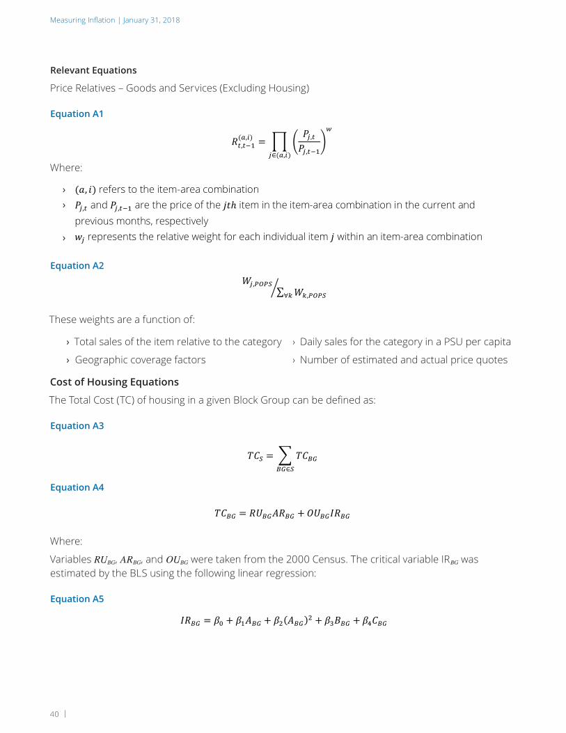
Measuring Inflation | January 31, 2018
40 |
Relevant Equations
Price Relatives – Goods and Services (Excluding Housing)
Equation A1
Where:
Equation A2
These weights are a function of:
› Total sales of the item relative to the category › Daily sales for the category in a PSU per capita
› Geographic coverage factors › Number of estimated and actual price quotes
Cost of Housing Equations
The Total Cost (TC) of housing in a given Block Group can be defined as:
Equation A3
Equation A4
Where:
Variables RUBG, ARBG, and OUBG were taken from the 2000 Census. The critical variable IRBG was estimated by the BLS using the following linear regression:
Equation A5
Inflation and Its Impact on Real Estate | October 31, 2017
Intellectual property of Unison Investment Management Proprietary and confidential Page 43 of 56
Telephone Point of Purchase Survey (TPOPS) The TPOPS survey is conducted by the Census Bureau, on behalf of the BLS, to aggregate information on where consumers are shopping and what they are buying. The survey is structured as 16 rotating questionnaires. Every four years a given PSU is either refreshed or will have a full new sample of data collected. A new TPOPS survey is initiated every quarter and run for four consecutive quarters. It selects 100–500 respondents (depending on PSU size) by randomly sampling phone numbers (landline and cellular). At each survey point, the respondents are asked to recall purchases made at various points in the past. These recall points range from as recently as the prior week to as long as five years before. The length of the recall window typically depends on the context of the good or service purchased (e.g., cars are purchased less frequently than groceries). Respondents are asked to report the amount of the purchase, the store name, and its location. The responses to this relatively small sample (20,000–40,000 people) produce the universe of store outlets from which the BLS samples22. Furthermore, the outlets selected are directly proportional to the size of the expenditures at these outlets. After the TPOPS data is cleaned and trimmed to remove outliers, store outlets are sampled by revenue weighting. The sample is supplemented with non-TPOPS outlets (e.g., electricity providers). Finally, sampled ELIs are matched with the sampled outlets. This gives specific item-outlet pairs to which field agents can assign price quotes collections.
Relevant Equations Price Relatives – Goods and Services (Excluding Housing) Equation A1
𝑅𝑅/,/FG(:,9) = H I
𝑃𝑃J,/𝑃𝑃J,/FG
KL
J∈(:,9)
Where: › (𝑎𝑎, 𝑖𝑖) refers to the item-area combination › 𝑃𝑃J,/ and 𝑃𝑃J,/FG are the price of the 𝑗𝑗𝑗𝑗ℎ item in the item-area combination in the current and
previous months, respectively › 𝑤𝑤J represents the relative weight for each individual item 𝑗𝑗 within an item-area combination
22 According to the BLS Handbook of Methods, the target number of respondents for each PSU is 200–400.
› ›
›
Inflation and Its Impact on Real Estate | October 31, 2017
Intellectual property of Unison Investment Management Proprietary and confidential Page 44 of 56
Equation A2
𝑊𝑊J,PQPR∑ 𝑊𝑊S,PQPR∀S
U
These weights are a function of:
› Total sales of the item relative to the category
› Daily sales for the category in a PSU per capita
› Geographic coverage factors
› Number of estimated and actual price quotes
Cost of Housing Equations The Total Cost (TC) of housing in a given Block Group can be defined as: Equation A3
𝑇𝑇𝐶𝐶R = X 𝑇𝑇𝐶𝐶YZYZ∈R
Equation A4
𝑇𝑇𝐶𝐶YZ = 𝑅𝑅𝑈𝑈YZ𝐴𝐴𝑅𝑅YZ + 𝑂𝑂𝑈𝑈YZ𝐼𝐼𝑅𝑅YZ Where:
› 𝑅𝑅𝑈𝑈YZ is the number of rental units in the Block Group
› 𝐴𝐴𝑅𝑅YZ is the average rent paid of the rental units in the Block Group
› 𝑂𝑂𝑈𝑈YZ is the number of owner-occupied units in the Block Group
› 𝐼𝐼𝑅𝑅YZ is the average imputed rent of the owner-occupied units in the Block Group as computed
by the BLS
Inflation and Its Impact on Real Estate | October 31, 2017
Intellectual property of Unison Investment Management Proprietary and confidential Page 45 of 56
Variables 𝑅𝑅𝑈𝑈YZ, 𝐴𝐴𝑅𝑅YZ,and 𝑂𝑂𝑈𝑈YZ were taken from the 2000 Census. The critical variable 𝐼𝐼𝑅𝑅YZ was estimated by the BLS using the following linear regression: Equation A5
𝐼𝐼𝑅𝑅YZ = 𝛽𝛽_ + 𝛽𝛽G𝐴𝐴YZ + 𝛽𝛽`(𝐴𝐴YZ)` + 𝛽𝛽a𝐵𝐵YZ + 𝛽𝛽c𝐶𝐶YZ
Where:
› 𝐴𝐴YZ is the average property value of owner-occupied housing units in the Block Group
› 𝐵𝐵YZ is the median income of homeowners in the Block Group
› 𝐶𝐶YZ is the average number of rooms for owner-occupied housing in the Block Group
Coefficients for this model were determined uniquely for each PSU. The regression step has the effect of smoothing out idiosyncrasies between individual blocks within a PSU. Specifically, it implies that rent can be reduced to a function of property value (with a square term to dampen rent for very high value homes with lower cap rates), income, and home size. These are likely adequate variables for explaining the majority variability in rent prices and will be robust to block level shocks. The probability of selection and index weighting of the segments are the inverse of one another: Equation A6
𝑃𝑃R =def∗hifj∑ deff∈ifj
and 𝑊𝑊R =∑ deff∈ifjdef∗hifj
Where 𝑛𝑛PRl is the number of segments to be chosen from each PSU. This implies that segments with high total housing costs have a higher probability of being selected and a lower weight. This has the effect of increasing the incidence of sampling geographical segments with a lot of market activity (and likely higher signal integrity). However, by increasing the incidence of these locales, a statistical increase in weight emerges. The inverse weighting step corrects those deviations, normalizing the sample. The importance of the 𝐼𝐼𝑅𝑅YZ estimation is also evident. It directly impacts the TC calculation, and thus segment selection probabilities and weights, which, as discussed below, are used to construct the OER index.

Unison Investment Management
41 |
Where:
› ABG is the average property value of owner-occupied housing units in the Block Group
› BBG is the median income of homeowners in the Block Group
› CBG is the average number of rooms for owner-occupied housing in the Block Group
Coefficients for this model were determined uniquely for each PSU. The regression step has the effect of smoothing out idiosyncrasies between individual blocks within a PSU. Specifically, it implies that rent can be reduced to a function of property value (with a square term to dampen rent for very high value homes with lower cap rates), income, and home size. These are likely adequate variables for explaining the majority variability in rent prices and will be robust to block level shocks.
The probability of selection and index weighting of the segments are the inverse of one another:
Equation A6
Where nPSU is the number of segments to be chosen from each PSU.
This implies that segments with high total housing costs have a higher probability of being selected and a lower weight. This has the effect of increasing the incidence of sampling geographical segments with a lot of market activity (and likely higher signal integrity). However, by increasing the incidence of these locales, a statistical increase in weight emerges. The inverse weighting step corrects those deviations, normalizing the sample.
› RUBG is the number of rental units in the Block Group
› ARBG is the average rent paid of the rental units in the Block Group
› OUBG is the number of owner-occupied units in the Block Group
› IRBG is the average imputed rent of the owner-occupied units in the Block Group as computed by the BLS
The importance of the IRBG estimation is also evident. It directly impacts the TC calculation, and thus segment selection probabilities and weights, which, as discussed below, are used to construct the OER index.
Economic and Pure Rents are defined as:
Equation A7
ERt = normalized rent ± other adjustments
ERt–6 = ERt – age bias ± analyst discretions
Equation A8
PRt = normalized rent – cost of utilites ± other adjustments
Inflation and Its Impact on Real Estate | October 31, 2017
Intellectual property of Unison Investment Management Proprietary and confidential Page 45 of 56
Variables 𝑅𝑅𝑈𝑈YZ, 𝐴𝐴𝑅𝑅YZ,and 𝑂𝑂𝑈𝑈YZ were taken from the 2000 Census. The critical variable 𝐼𝐼𝑅𝑅YZ was estimated by the BLS using the following linear regression: Equation A5
𝐼𝐼𝑅𝑅YZ = 𝛽𝛽_ + 𝛽𝛽G𝐴𝐴YZ + 𝛽𝛽`(𝐴𝐴YZ)` + 𝛽𝛽a𝐵𝐵YZ + 𝛽𝛽c𝐶𝐶YZ
Where:
› 𝐴𝐴YZ is the average property value of owner-occupied housing units in the Block Group
› 𝐵𝐵YZ is the median income of homeowners in the Block Group
› 𝐶𝐶YZ is the average number of rooms for owner-occupied housing in the Block Group
Coefficients for this model were determined uniquely for each PSU. The regression step has the effect of smoothing out idiosyncrasies between individual blocks within a PSU. Specifically, it implies that rent can be reduced to a function of property value (with a square term to dampen rent for very high value homes with lower cap rates), income, and home size. These are likely adequate variables for explaining the majority variability in rent prices and will be robust to block level shocks. The probability of selection and index weighting of the segments are the inverse of one another: Equation A6
𝑃𝑃R =def∗hifj∑ deff∈ifj
and 𝑊𝑊R =∑ deff∈ifjdef∗hifj
Where 𝑛𝑛PRl is the number of segments to be chosen from each PSU. This implies that segments with high total housing costs have a higher probability of being selected and a lower weight. This has the effect of increasing the incidence of sampling geographical segments with a lot of market activity (and likely higher signal integrity). However, by increasing the incidence of these locales, a statistical increase in weight emerges. The inverse weighting step corrects those deviations, normalizing the sample. The importance of the 𝐼𝐼𝑅𝑅YZ estimation is also evident. It directly impacts the TC calculation, and thus segment selection probabilities and weights, which, as discussed below, are used to construct the OER index.

Measuring Inflation | January 31, 2018
42 |
Equation A9
PRt–6 = PRt – age bias ± analyst discretions
The following are estimated for each segment:
› Imputed Rents (IR) › Average Rents (AR)
› Counts of Rental Units (RU) › Counts of Owner-Occupied Units (OU)
› Economic Rents (ER, over time) › Pure Rents (PR, over time)
The renter weight for a given unit is simply the segment weight (the weight of that geographic location) times the number of renters in the segment:
Equation A10
The owner weight is conceptually similar to the renter weight, but is scaled by the segment ratio of estimated average imputed rent of owner-occupied units to the average rent of a rental:
Equation A11
The definition of OWS reiterates the importance in the estimation of the imputed rent. It is present twice in the equation, explicitly in the scaling ratio and in WS, which is a function of TC. Intuitively, the weights ensure that the changes in price levels by sample are properly allocated between renters and owners.
Finally, the price relatives are defined as the weighted sum of this measurement period’s rents relative to that of the previous measurement period. In particular, for a given CPI area (PSU or higher level):
Equation A12
Equation A13
These six-month relatives are then transformed to one-month relatives by taking the sixth root. This also has the effect of smoothing the series.
Inflation and Its Impact on Real Estate | October 31, 2017
Intellectual property of Unison Investment Management Proprietary and confidential Page 46 of 56
Economic and Pure Rents are defined as: Equation A7
𝐸𝐸𝑅𝑅/ = 𝑛𝑛𝑛𝑛𝑛𝑛𝑛𝑛𝑛𝑛𝑛𝑛𝑛𝑛𝑛𝑛𝑛𝑛𝑛𝑛𝑛𝑛𝑛𝑛𝑛𝑛𝑟𝑟 ± 𝑛𝑛𝑟𝑟ℎ𝑛𝑛𝑛𝑛𝑛𝑛𝑛𝑛𝑎𝑎𝑎𝑎𝑎𝑎𝑟𝑟𝑛𝑛𝑛𝑛𝑛𝑛𝑟𝑟𝑎𝑎 𝐸𝐸𝑅𝑅/Fx = 𝐸𝐸𝑅𝑅/ − 𝑛𝑛𝑎𝑎𝑛𝑛𝑏𝑏𝑛𝑛𝑛𝑛𝑎𝑎 ± 𝑛𝑛𝑛𝑛𝑛𝑛𝑛𝑛𝑎𝑎𝑎𝑎𝑟𝑟𝑛𝑛𝑛𝑛𝑎𝑎𝑑𝑑𝑛𝑛𝑛𝑛𝑟𝑟𝑛𝑛𝑛𝑛𝑛𝑛𝑎𝑎
Equation A8
𝑃𝑃𝑅𝑅/ = 𝑛𝑛𝑛𝑛𝑛𝑛𝑛𝑛𝑛𝑛𝑛𝑛𝑛𝑛𝑛𝑛𝑛𝑛𝑛𝑛𝑛𝑛𝑛𝑛𝑛𝑛𝑟𝑟 − 𝑑𝑑𝑛𝑛𝑎𝑎𝑟𝑟𝑛𝑛𝑜𝑜𝑎𝑎𝑟𝑟𝑛𝑛𝑛𝑛𝑛𝑛𝑟𝑟𝑛𝑛𝑎𝑎 ± 𝑛𝑛𝑟𝑟ℎ𝑛𝑛𝑛𝑛𝑛𝑛𝑛𝑛𝑎𝑎𝑎𝑎𝑎𝑎𝑟𝑟𝑛𝑛𝑛𝑛𝑛𝑛𝑟𝑟𝑎𝑎
Equation A9
𝑃𝑃𝑅𝑅/Fx = 𝑃𝑃𝑅𝑅/ − 𝑛𝑛𝑎𝑎𝑛𝑛𝑏𝑏𝑛𝑛𝑛𝑛𝑎𝑎 ± 𝑛𝑛𝑛𝑛𝑛𝑛𝑛𝑛𝑎𝑎𝑎𝑎𝑟𝑟𝑛𝑛𝑛𝑛𝑎𝑎𝑑𝑑𝑛𝑛𝑛𝑛𝑟𝑟𝑛𝑛𝑛𝑛𝑛𝑛𝑎𝑎 The following are estimated for each segment:
› Imputed Rents (IR) › Average Rents (AR) › Counts of Rental Units (RU) › Counts of Owner-Occupied Units (OU) › Economic Rents (ER, over time) › Pure Rents (PR, over time)
The renter weight for a given unit is simply the segment weight (the weight of that geographic location) times the number of renters in the segment: Equation A10
𝑅𝑅𝑊𝑊R = 𝑊𝑊R𝑅𝑅𝑅𝑅R The owner weight is conceptually similar to the renter weight, but is scaled by the segment ratio of estimated average imputed rent of owner-occupied units to the average rent of a rental: Equation A11
𝑂𝑂𝑊𝑊R = 𝑊𝑊R𝑂𝑂𝑅𝑅R ~𝐼𝐼𝑅𝑅R𝐴𝐴𝑅𝑅R
�
The definition of 𝑂𝑂𝑊𝑊R reiterates the importance in the estimation of the imputed rent. It is present twice in the equation, explicitly in the scaling ratio and in 𝑊𝑊R, which is a function of TC. Intuitively, the weights ensure that the changes in price levels by sample are properly allocated between renters and owners.
Inflation and Its Impact on Real Estate | October 31, 2017
Intellectual property of Unison Investment Management Proprietary and confidential Page 47 of 56
Finally, the price relatives are defined as the weighted sum of this measurement period’s rents relative to that of the previous measurement period. In particular, for a given CPI area (PSU or higher level): Equation A12
𝑅𝑅𝑅𝑅𝑙𝑙1ÄÅ:,/,/FxÇÉÑd =∑ (∑ 𝑅𝑅𝑅𝑅R𝐸𝐸𝑅𝑅R,9,/)9∈RR∈1ÄÅ:∑ (∑ 𝑅𝑅𝑅𝑅R𝐸𝐸𝑅𝑅R,9,/Fx)9∈RR∈1ÄÅ:
Equation A13
𝑅𝑅𝑅𝑅𝑙𝑙1ÄÅ:,/,/FxQÉÇ =∑ (∑ 𝑂𝑂𝑅𝑅R𝑃𝑃𝑅𝑅R,9,/)9∈RR∈1ÄÅ:∑ (∑ 𝑂𝑂𝑅𝑅R𝑃𝑃𝑅𝑅R,9,/Fx)9∈RR∈1ÄÅ:
These six-month relatives are then transformed to one-month relatives by taking the sixth root. This also has the effect of smoothing the series. Equation A14
𝑅𝑅𝑅𝑅𝑙𝑙1ÄÅ:,/,/FGÇÉÑd = Ö𝑅𝑅𝑅𝑅𝑙𝑙1ÄÅ:,/,/FGÇÉÑdÜ
Equation A15
𝑅𝑅𝑅𝑅𝑙𝑙1ÄÅ:,/,/FGQÉÇ = Ö𝑅𝑅𝑅𝑅𝑙𝑙1ÄÅ:,/,/FGQÉÇÜ
Vacant sample units that were previously occupied and non-interviewed units are factored in to the above derivation. Vacant unit rents are imputed by assuming a jump rate that can vary based on location. Non-interviewed unit rents are also imputed by assuming an average continuous rate of rent change at one of three different rent-level categories (high, medium, or low). The one-month price relatives are then used to move the CPI elementary indexes, as with other item-area combinations. Equation A16
𝐼𝐼𝐼𝐼𝑋𝑋1ÄÅ:,/0 = 𝐼𝐼𝐼𝐼𝑋𝑋1ÄÅ:,/FG0 𝑅𝑅𝐸𝐸𝐿𝐿1ÄÅ:,/,/FG0 𝐼𝐼 ∈ 𝑅𝑅𝐸𝐸𝑅𝑅𝑅𝑅,𝑂𝑂𝐸𝐸𝑅𝑅 These are then aggregated up to yield the final CPI-U Rent and OER indexes.
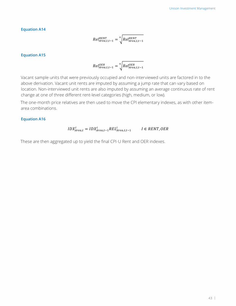
Unison Investment Management
43 |
Inflation and Its Impact on Real Estate | October 31, 2017
Intellectual property of Unison Investment Management Proprietary and confidential Page 47 of 56
Finally, the price relatives are defined as the weighted sum of this measurement period’s rents relative to that of the previous measurement period. In particular, for a given CPI area (PSU or higher level): Equation A12
𝑅𝑅𝑅𝑅𝑙𝑙1ÄÅ:,/,/FxÇÉÑd =∑ (∑ 𝑅𝑅𝑅𝑅R𝐸𝐸𝑅𝑅R,9,/)9∈RR∈1ÄÅ:∑ (∑ 𝑅𝑅𝑅𝑅R𝐸𝐸𝑅𝑅R,9,/Fx)9∈RR∈1ÄÅ:
Equation A13
𝑅𝑅𝑅𝑅𝑙𝑙1ÄÅ:,/,/FxQÉÇ =∑ (∑ 𝑂𝑂𝑅𝑅R𝑃𝑃𝑅𝑅R,9,/)9∈RR∈1ÄÅ:∑ (∑ 𝑂𝑂𝑅𝑅R𝑃𝑃𝑅𝑅R,9,/Fx)9∈RR∈1ÄÅ:
These six-month relatives are then transformed to one-month relatives by taking the sixth root. This also has the effect of smoothing the series. Equation A14
𝑅𝑅𝑅𝑅𝑙𝑙1ÄÅ:,/,/FGÇÉÑd = Ö𝑅𝑅𝑅𝑅𝑙𝑙1ÄÅ:,/,/FGÇÉÑdÜ
Equation A15
𝑅𝑅𝑅𝑅𝑙𝑙1ÄÅ:,/,/FGQÉÇ = Ö𝑅𝑅𝑅𝑅𝑙𝑙1ÄÅ:,/,/FGQÉÇÜ
Vacant sample units that were previously occupied and non-interviewed units are factored in to the above derivation. Vacant unit rents are imputed by assuming a jump rate that can vary based on location. Non-interviewed unit rents are also imputed by assuming an average continuous rate of rent change at one of three different rent-level categories (high, medium, or low). The one-month price relatives are then used to move the CPI elementary indexes, as with other item-area combinations. Equation A16
𝐼𝐼𝐼𝐼𝑋𝑋1ÄÅ:,/0 = 𝐼𝐼𝐼𝐼𝑋𝑋1ÄÅ:,/FG0 𝑅𝑅𝐸𝐸𝐿𝐿1ÄÅ:,/,/FG0 𝐼𝐼 ∈ 𝑅𝑅𝐸𝐸𝑅𝑅𝑅𝑅,𝑂𝑂𝐸𝐸𝑅𝑅 These are then aggregated up to yield the final CPI-U Rent and OER indexes.
Equation A14
Equation A15
Vacant sample units that were previously occupied and non-interviewed units are factored in to the above derivation. Vacant unit rents are imputed by assuming a jump rate that can vary based on location. Non-interviewed unit rents are also imputed by assuming an average continuous rate of rent change at one of three different rent-level categories (high, medium, or low).
The one-month price relatives are then used to move the CPI elementary indexes, as with other item-area combinations.
Equation A16
These are then aggregated up to yield the final CPI-U Rent and OER indexes.
Inflation and Its Impact on Real Estate | October 31, 2017
Intellectual property of Unison Investment Management Proprietary and confidential Page 47 of 56
Finally, the price relatives are defined as the weighted sum of this measurement period’s rents relative to that of the previous measurement period. In particular, for a given CPI area (PSU or higher level): Equation A12
𝑅𝑅𝑅𝑅𝑙𝑙1ÄÅ:,/,/FxÇÉÑd =∑ (∑ 𝑅𝑅𝑅𝑅R𝐸𝐸𝑅𝑅R,9,/)9∈RR∈1ÄÅ:∑ (∑ 𝑅𝑅𝑅𝑅R𝐸𝐸𝑅𝑅R,9,/Fx)9∈RR∈1ÄÅ:
Equation A13
𝑅𝑅𝑅𝑅𝑙𝑙1ÄÅ:,/,/FxQÉÇ =∑ (∑ 𝑂𝑂𝑅𝑅R𝑃𝑃𝑅𝑅R,9,/)9∈RR∈1ÄÅ:∑ (∑ 𝑂𝑂𝑅𝑅R𝑃𝑃𝑅𝑅R,9,/Fx)9∈RR∈1ÄÅ:
These six-month relatives are then transformed to one-month relatives by taking the sixth root. This also has the effect of smoothing the series. Equation A14
𝑅𝑅𝑅𝑅𝑙𝑙1ÄÅ:,/,/FGÇÉÑd = Ö𝑅𝑅𝑅𝑅𝑙𝑙1ÄÅ:,/,/FGÇÉÑdÜ
Equation A15
𝑅𝑅𝑅𝑅𝑙𝑙1ÄÅ:,/,/FGQÉÇ = Ö𝑅𝑅𝑅𝑅𝑙𝑙1ÄÅ:,/,/FGQÉÇÜ
Vacant sample units that were previously occupied and non-interviewed units are factored in to the above derivation. Vacant unit rents are imputed by assuming a jump rate that can vary based on location. Non-interviewed unit rents are also imputed by assuming an average continuous rate of rent change at one of three different rent-level categories (high, medium, or low). The one-month price relatives are then used to move the CPI elementary indexes, as with other item-area combinations. Equation A16
𝐼𝐼𝐼𝐼𝑋𝑋1ÄÅ:,/0 = 𝐼𝐼𝐼𝐼𝑋𝑋1ÄÅ:,/FG0 𝑅𝑅𝐸𝐸𝐿𝐿1ÄÅ:,/,/FG0 𝐼𝐼 ∈ 𝑅𝑅𝐸𝐸𝑅𝑅𝑅𝑅,𝑂𝑂𝐸𝐸𝑅𝑅 These are then aggregated up to yield the final CPI-U Rent and OER indexes.
Measuring Inflation | January 31, 2018
44 |
Appendix II: Alternative Methods for Calculating Homeownership Costs
Several methods for measuring the cost of owner-occupied housing have been researched over the years. The BLS tested experimental CPI indexes that included variations of the User Cost and OER approaches in the early 1980s. Before switching to an OER method, the BLS employed a Cost of Purchase method, which is utilized by Australia and New Zealand in their measures of inflation. More than a third of OECD countries use a rental equivalence approach, while nine simply exclude owner-occupied housing from CPI.
User Cost ApproachA User Cost approach to measure owner-occupied housing costs sets up a one-period framework in which a household:
› Purchases a home at t=0
› Consumes the services the home provides and incurs costs due to maintenance and taxes
› Sells the home at t=T
The household has a net consumption yield over the period, and experiences a small capital gain or loss at the end of the period through the resale of the home. The spirit of this model is commonly used in other settings, such as capital asset pricing. Assuming a frictionless world, the User Cost can be defined as:
Equation A17
Where:
The theory implies that, at equilibrium in this frictionless world, owner-occupied user costs should equal the rental price of the home. This value should also be equivalent to the rent received (paid) by the landlord (tenant). Yet, the frictions of the real-world introduce several challenges. Variables such as expected home price appreciation, depreciation, tax treatments, and nominal interest rate, among others, must be estimated or identified. Depending on these assumptions, user costs can be highly volatile. They can even be negative if expected HPA is substantially higher than the nominal interest rate, which is not unrealistic in certain regions given today’s low-rate environment.
Debate over whether the method is conceptually appropriate for a CPI measure also exists. This is an outgrowth of the fact that interest rates and home prices (investment-like features) are reflected in this framework. Moreover, utilizing this method requires finding a balance between an intractable complex model, which is infeasible to implement, and a simplified version, such as the one defined above, that requires an unreasonable number of assumptions and yields counterintuitive results.
Inflation and Its Impact on Real Estate | October 31, 2017
Intellectual property of Unison Investment Management Proprietary and confidential Page 48 of 56
Appendix II: Alternative Methods for Calculating Homeownership Costs Several methods for measuring the cost of owner-occupied housing have been researched over the years. The BLS tested experimental CPI indexes that included variations of the User Cost and OER approaches in the early 1980s. Before switching to an OER method, the BLS employed a Cost of Purchase method, which is utilized by Australia and New Zealand in their measures of inflation. More than a third of OECD countries use a rental equivalence approach, while nine simply exclude owner-occupied housing from CPI. User Cost Approach
A User Cost approach to measure owner-occupied housing costs sets up a one-period framework in which a household:
› Purchases a home at t=0
› Consumes the services the home provides and incurs costs due to maintenance and taxes
› Sells the home at t=T
The household has a net consumption yield over the period, and experiences a small capital gain or loss at the end of the period through the resale of the home. The spirit of this model is commonly used in other settings, such as capital asset pricing. Assuming a frictionless world, the User Cost can be defined as: Equation A177
𝑈𝑈𝐶𝐶/ = 𝑃𝑃/(𝑟𝑟/ + 𝛾𝛾 − 𝔼𝔼[𝑝𝑝]) Where:
› 𝑃𝑃/ is the value of the home › 𝑟𝑟/ is the nominal interest rate › 𝛾𝛾 is a catchall for depreciation, maintenance, and tax rates › 𝔼𝔼[𝑝𝑝] is the expected appreciation of the home over the period
The theory implies that, at equilibrium in this frictionless world, owner-occupied user costs should equal the rental price of the home. This value should also be equivalent to the rent received (paid) by the landlord (tenant). Yet, the frictions of the real-world introduce several challenges. Variables such as expected home price appreciation, depreciation, tax treatments, and nominal interest rate, among others, must be estimated or identified. Depending on these assumptions, user costs can be highly
› › › ›
Inflation and Its Impact on Real Estate | October 31, 2017
Intellectual property of Unison Investment Management Proprietary and confidential Page 48 of 56
Appendix II: Alternative Methods for Calculating Homeownership Costs Several methods for measuring the cost of owner-occupied housing have been researched over the years. The BLS tested experimental CPI indexes that included variations of the User Cost and OER approaches in the early 1980s. Before switching to an OER method, the BLS employed a Cost of Purchase method, which is utilized by Australia and New Zealand in their measures of inflation. More than a third of OECD countries use a rental equivalence approach, while nine simply exclude owner-occupied housing from CPI. User Cost Approach
A User Cost approach to measure owner-occupied housing costs sets up a one-period framework in which a household:
› Purchases a home at t=0
› Consumes the services the home provides and incurs costs due to maintenance and taxes
› Sells the home at t=T
The household has a net consumption yield over the period, and experiences a small capital gain or loss at the end of the period through the resale of the home. The spirit of this model is commonly used in other settings, such as capital asset pricing. Assuming a frictionless world, the User Cost can be defined as: Equation A177
𝑈𝑈𝐶𝐶/ = 𝑃𝑃/(𝑟𝑟/ + 𝛾𝛾 − 𝔼𝔼[𝑝𝑝]) Where:
› 𝑃𝑃/ is the value of the home › 𝑟𝑟/ is the nominal interest rate › 𝛾𝛾 is a catchall for depreciation, maintenance, and tax rates › 𝔼𝔼[𝑝𝑝] is the expected appreciation of the home over the period
The theory implies that, at equilibrium in this frictionless world, owner-occupied user costs should equal the rental price of the home. This value should also be equivalent to the rent received (paid) by the landlord (tenant). Yet, the frictions of the real-world introduce several challenges. Variables such as expected home price appreciation, depreciation, tax treatments, and nominal interest rate, among others, must be estimated or identified. Depending on these assumptions, user costs can be highly

Unison Investment Management
45 |
Much research has already been done on this method as it relates to accounting for owner-occupied housing costs in inflation. Some consider it the only reasonable alternative to a rental equivalency method, yet more work is needed before this approach becomes a serious contender for use in CPI. The idea of an “Opportunity Cost” approach—one in which a hypothetical homeowner is faced with the choice of either continuing to own or rent out her residence over a given period—has been researched in recent years. It is a combination of rental equivalency and a variation of the User Cost method. Each is used to produce, respectively, a rental opportunity cost index (ROC) and an owner-occupied opportunity cost index (OOC). Since the hypothetical homeowner is assumed to be rational, they will choose the best option between renting and continue to own. Thus, the owner-occupied cost index in a given period is the maximum of ROC and OOC.
Cost of Purchase: Asset Price RevisitedMany researchers and academics support the change to an OER measure and feel that it was a dramatic improvement over the previous Asset Price method. However, several issues associated with the former approach could be considered by-products of the times. The method could be substantially improved if implemented today, because of the following:
› House Price Data Availability: At the time when the Asset Price method was abandoned, Case and Shiller had yet to publish their seminal paper on house price indexes constructed using repeat sales. Today, countless house price indexes are produced on a monthly basis. Despite having known limitations, Case-Shiller repeat sales indexes for the nation and select CBSAs are readily available. Freddie Mac and other government agencies release similar series on a wider geography. Companies, such as Black Knight and CoreLogic, produce indexes on more focused geographic areas (e.g., zip codes, Census Tracts, etc.). More companies are entering this space, combining alternative data sets with sales transactions to design the next best index or valuation model. Moreover, MLS and appraisal data has become more accessible and can provide the most up-to-date information on markets from national down to neighborhood geographies.
› Weight Calibration: The expenditure weights used in the 1970s were outdated and arguably flawed in their construction. With more data available, both on macro (through aggregated accounts) and micro levels (through more frequent and better designed surveys), the expenditure weights for housing could be updated more frequently. The BLS still seems to struggle with this; the BEA supplements CEX data with American Housing Survey (AHS) and American Community Survey (ACS) data. These surveys are conducted more frequently than the CEX and capture important housing expenditure information.
› Sample Size: The sample in the old method was limited to a subset of only those who purchased a home in a measurement month. Those who had previously purchased a home were not included in the cost calculation, yet they were most likely making mortgage payments. New data sources could be leveraged to creatively expand this sample. Loan level data reveals recent purchases of homes, including the type of mortgage product and interest rate. In addition, the data shows payment patterns of previous purchasers. Since a relatively small number of households purchase a home in a given month, including this additional data would expand the sample to compute the costs borne by the average homeowner.

Measuring Inflation | January 31, 2018
46 |
› Volatility: Interest rate movements continue to add volatility to the overall price index. Smoothing methods, such as taking a moving average, have been experimented with in the past. Using any type of smoothing technique would result in a trade-off of reduced volatility for a slight bias in the measure of current costs for homeowners. Using the prevailing market rate for the month could also be considered. Even today, the volatile food and energy components of CPI-U are commonly removed to provide a “Core” CPI number.
Intuitively, required down payment and anticipated monthly mortgage payments should be considered in the cost of homeownership. The concept of “home affordability” precisely attempts to measure this at any given time. Naturally, these factors should be included in an index that measures consumer prices, and the Cost of Purchase method achieves this.

Unison Investment Management
47 |
Appendix III: The Phillips Curve
W.H. Phillips studied wage inflation and unemployment in the United Kingdom from 1861 to 1957. From his work, he established the existence of a significant and material inverse relationship between inflation and unemployment. This makes intuitive sense and has been the bedrock of US Fiscal Policy for many decades.
Over the years, the Phillips Curve has been examined from several different perspectives. In 1968, Milton Friedman called the Phillips Curve nonsense23. He believed that it was only valid in nominal terms, if at all, and that rational workers should be fixated on the real rate of wages rather than nominal levels of wages. Keynesians, upon whose philosophy the Phillips Curve is built, believed that there were no circumstances under which an economy could experience both high unemployment and high inflation. This was proved to be incorrect in 1970.
However, the Phillips Curve established that there is likely a level of unemployment which can be maintained if inflation is low and stable. This forms the basis of modern Fed policy. The challenges of what constitutes inflation and how that relates to wage inflation and unemployment are debatable.
Source: Economics Discussion – The Phillips Curve Explained
23. John Phelan, “Milton Friedman and the rise and fall of the Phillips Curve,” the commentator, 2012 http://www.thecommentator.com/article/1895/milton_friedman_and_the_rise_and_fall_of_the_phillips_curve

Measuring Inflation | January 31, 2018
48 |
Appendix IV: What is PCE and how does it differ from CPI?
The Personal Consumption Expenditure (PCE) price index is another measure of the change in prices for consumers. It is maintained by the US Bureau of Economic Analysis (BEA) and is an input in
the US GDP figure. The PCE index draws much attention since its core version (excluding food and fuel) is the preferred measure of inflation of the Federal Reserve. The PCE index and CPI are highly correlated, with a coefficient of nearly 1.0; the elementary indexes of the CPI-U are used as inputs in the PCE index construction. However, there exist important differences between the two that lead to divergences of the series over long periods of time.
In general, the annual growth rate of the CPI has been higher than that of the PCE index. CPI has, however, shown prices falling faster in times when inflation rapidly decreases, as in 2015, or during periods of deflation, as in 2009. These differences can be attributed to:
› Formula Effects › Differences in Weights
› Mismatch of Scoped Items
Formula EffectsThe CPI uses a version of the Laspeyres price formula, which measures the price relative by setting the quantity of goods in the measurement period as that in the base period. Using Q as the base period, this is formally defined as:
Equation A18
Figure A2. PCE and CPI Monthly YoY Percent Change
Inflation and Its Impact on Real Estate | October 31, 2017
Intellectual property of Unison Investment Management Proprietary and confidential Page 52 of 56
Appendix IV: What is PCE and how does it differ from CPI?
The Personal Consumption Expenditure (PCE) price index is another measure of the change in prices for consumers. It is maintained by the US Bureau of Economic Analysis (BEA) and is an input in the US GDP figure. The PCE index draws much attention since its core version (excluding food and fuel) is the preferred measure of inflation of the Federal Reserve. The PCE index and CPI are highly correlated, with a coefficient of nearly 1.0; the elementary indexes of the CPI-U are used as inputs in the PCE index construction. However, there exist important differences between the two that lead to divergences of the series over long periods of time. Figure A2. PCE and CPI Monthly YoY Percent Change
In general, the annual growth rate of the CPI has been higher than that of the PCE index. CPI has, however, shown prices falling faster in times when inflation rapidly decreases, as in 2015, or during periods of deflation, as in 2009. These differences can be attributed to:
› Formula Effects
› Differences in Weights
› Mismatch of Scoped Items
-3%
-2%
-1%
0%
1%
2%
3%
4%
5%
6%
2000
2001
2002
2003
2004
2005
2006
2007
2008
2009
2010
2011
2012
2013
2014
2015
2016
2017
YoY
Chan
ge
Delta CPI-U PCE
Inflation and Its Impact on Real Estate | October 31, 2017
Intellectual property of Unison Investment Management Proprietary and confidential Page 53 of 56
Formula Effects
The CPI uses a version of the Laspeyres price formula, which measures the price relative by setting the quantity of goods in the measurement period as that in the base period. Using 𝑡𝑡 as the base period, this is formally defined as: Equation A188
𝐿𝐿/,/çG =∑ 𝑃𝑃9,/çG𝑄𝑄9,/9∑ 𝑃𝑃9,/𝑄𝑄9,/9
The base period is updated every two years for most elementary CPI indexes. The PCE price index utilizes the Fisher-Ideal formulation, which is a weighted average of the Laspeyres and Paasche price relatives. While the Laspeyres uses the base period quantity, the Paasche assumes 𝑄𝑄 to be the quantity in the measurement period. Equation A19
𝑃𝑃/,/çG =∑ 𝑃𝑃9,/çG𝑄𝑄9,/çG9∑ 𝑃𝑃9,/𝑄𝑄9,/çG9
And yields: Equation A190
𝐹𝐹/,/çG = è𝐿𝐿/,/çG𝑃𝑃/,/çGêG/`
Since the PCE index is chained, the relatives are multiplied together to yield the index level. Equation A201
𝐹𝐹/çG = 𝐹𝐹_,G𝐹𝐹G,` …𝐹𝐹/FG,/𝐹𝐹/,/çG The chaining of the Fisher-Ideal price relatives will generally lead to a smaller change, since the Laspeyres type price relative is usually higher than the Paasche version. This effect accounts for almost half of the difference in growth rates between CPI and the PCE. The use of the Fisher-Ideal is intended to better capture substitution effects since quantities of goods in the measurement period (t+1) are accounted for through the Paasche price relative; however, these data are hard to gather and are

Unison Investment Management
49 |
Equation A19
And yields:
Equation A20
Since the PCE index is chained, the relatives are multiplied together to yield the index level.
Equation A21
The chaining of the Fisher-Ideal price relatives will generally lead to a smaller change, since the Laspeyres type price relative is usually higher than the Paasche version. This effect accounts for almost half of the difference in growth rates between CPI and the PCE. The use of the Fisher-Ideal is intended to better capture substitution effects since quantities of goods in the measurement period (t+1) are accounted for through the Paasche price relative; however, these data are hard to gather and are oftentimes unavailable.
Differences in WeightsThe two indexes leverage different data sources when computing expenditure weights, which ultimately contribute slight variation in index levels. The BLS uses the CEX to base the CPI relative weights, while the BEA uses several business surveys, including Census Bureau retail surveys and the Quarterly Services Survey. The base surveys used to weight the indexes vary in terms of respondents (strictly consumers vs. some business owner contribution) as well as survey release frequency. The difference in the Rent of Shelter component relative weights accounts for a significant amount of overall discrepancy between the two series. This is not surprising given that Rent of Shelter is a sizeable proportion of the overall price index and any deviation would have a noticeable impact.
Mismatch of Scoped ItemsThe item coverage of the two series does not perfectly overlap. The CPI attempts to measure consumer expenditures of urban households. The PCE index also factors in the expenditures of nonprofit institutions, and measures this consumption in a way that is rolled into the BEA GDP calculation. This leads to the inclusion of some items in one index and not the other. Examples range from the inconsequential—Food away from home (CPI) vs. Food on farms (PCE)—to fundamental: the inclusion of employer-paid medical benefits and net foreign remittances (PCE).
Other notable effects also contribute to the difference between the two series. These include differences in the construction of specific components and the way seasonality is handled. Regarding the cost of owner-occupied housing, the BEA leverages the same rental equivalence method that the BLS uses in the CPI. As mentioned above, the BEA uses alternative surveys as data sources. For Rent of Shelter, they use rents from the Residential Finance Survey and the home values American Housing Surveys. In addition to using the same methodology, the BLS OER series is itself used in the construction of the BEA series, so the two series are very closely related.
Inflation and Its Impact on Real Estate | October 31, 2017
Intellectual property of Unison Investment Management Proprietary and confidential Page 53 of 56
Formula Effects
The CPI uses a version of the Laspeyres price formula, which measures the price relative by setting the quantity of goods in the measurement period as that in the base period. Using 𝑡𝑡 as the base period, this is formally defined as: Equation A188
𝐿𝐿/,/çG =∑ 𝑃𝑃9,/çG𝑄𝑄9,/9∑ 𝑃𝑃9,/𝑄𝑄9,/9
The base period is updated every two years for most elementary CPI indexes. The PCE price index utilizes the Fisher-Ideal formulation, which is a weighted average of the Laspeyres and Paasche price relatives. While the Laspeyres uses the base period quantity, the Paasche assumes 𝑄𝑄 to be the quantity in the measurement period. Equation A19
𝑃𝑃/,/çG =∑ 𝑃𝑃9,/çG𝑄𝑄9,/çG9∑ 𝑃𝑃9,/𝑄𝑄9,/çG9
And yields: Equation A190
𝐹𝐹/,/çG = è𝐿𝐿/,/çG𝑃𝑃/,/çGêG/`
Since the PCE index is chained, the relatives are multiplied together to yield the index level. Equation A201
𝐹𝐹/çG = 𝐹𝐹_,G𝐹𝐹G,` …𝐹𝐹/FG,/𝐹𝐹/,/çG The chaining of the Fisher-Ideal price relatives will generally lead to a smaller change, since the Laspeyres type price relative is usually higher than the Paasche version. This effect accounts for almost half of the difference in growth rates between CPI and the PCE. The use of the Fisher-Ideal is intended to better capture substitution effects since quantities of goods in the measurement period (t+1) are accounted for through the Paasche price relative; however, these data are hard to gather and are

Measuring Inflation | January 31, 2018
50 |
ReferencesThe BLS Handbook of Methods, “Chapter 17. The Consumer Price Index (Updated 06/2015),” U.S. Bureau of Labor Statistics, June 2015, https://www.bls.gov/opub/hom/pdf/homch17.pdf.
Cagan, Phillip and Moore, Geoffrey H., “Some proposals to improve the Consumer Price Index,” The Consumer Price Index: Issues and Alternatives, American Enterprise Institute for Public Policy Research, September 1981, https://www.bls.gov/opub/mlr/1981/09/art3full.pdf.
Church, Jonathan, “Explaining the 30-year shift in consumer expenditures from commodities to services, 1982–2012,” Monthly Labor Review, U.S. Bureau of Labor Statistics, April 2014, https://doi.org/10.21916/mlr.2014.17.
Concepts and Methods of the U.S. National Income and Product Accounts. “Chapter 5: Personal Consumption Expenditures,” U.S. Bureau of Economic Analysis, October 2016. https://bea.gov/national/pdf/chapter5.pdf.
Díaz, Antonia, Luengo-Prado, María José, “On the user cost and homeownership,” Review of Economic Dynamics, Volume 11, Issue 3, 2008, Pages 584-613, ISSN 1094-2025, http://dx.doi.org/10.1016/j.red.2007.12.002.
Diewert, W. Erwin and Nakamura, Alice Orcutt, “Accounting for Housing in a CPI,” FRB of Philadelphia Working Paper No. 09-4, 1999, Available at SSRN: https://ssrn.com/abstract=1367631.
The Economist, “Measuring Inflation: How much is that doggy?” The Economist print edition, Finance and economics, March 17, 2016.
The Economist, “Measuring economies: The trouble with GDP,” The Economist print edition, Briefing, April 30, 2016.
Garner, Thesia I., Verbrugge, Randal, “The Puzzling Divergence of U.S. Rents and User Costs, 1908-2004: Summary and Extensions,” BLS Working Papers, U.S. Bureau of Labor Statistics, October 2007.
Lane, Walter F., Randolph, William C., and Berenson, Stephen A., “Adjusting the CPI shelter index to compensate for effect of depreciation,” BLS Handbook of Methods, Technical Notes, U.S. Bureau of Labor Statistics, pages 34-37. October 2010, https://www.bls.gov/opub/mlr/1988/10/rpt1full.pdf.
Mayerhauser, N. and Reinsdorf, M., “Housing Services in the National Economic Accounts,” U.S. Bureau of Economic Analysis, Updated as of September, 2007.
McCully, Clinton P., Moyer, Brian C., and Stewart, Kenneth J., “Comparing the Consumer Price Index and the Personal Consumption Expenditures Price Index,” U.S. Bureau of Economic Analysis, November, 2007, https://www.bea.gov/scb/pdf/2007/11%20November/1107_cpipce.pdf.
____ “A reconciliation between the Consumer Price Index and the Personal Consumption Expenditures price index,” U.S. Bureau of Economic Analysis and U.S. Bureau of Labor Statistics, September 2007, https://www.bea.gov/papers/pdf/cpi_pce.pdf.
Norwood, Janet L., “Two Consumer Price Index issues: weighting and homeownership,” The Anatomy of Price Change, U.S. Bureau of Labor Statistics, March 1981, pages 58-59, https://www.bls.gov/opub/mlr/1981/03/rpt1full.pdf.
Reed, Stephen, “One hundred years of price change: the Consumer Price Index and the American inflation experience,” Monthly Labor Review, U.S. Bureau of Labor Statistics, April 2014, https://doi.org/10.21916/mlr.2014.14.
Rippy, Darren, “The first hundred years of the Consumer Price Index: a methodological and political history,” Monthly Labor Review, U.S. Bureau of Labor Statistics, April 2014, https://doi.org/10.21916/mlr.2014.13.
Paben, Steven, Johnson, William, and Schilp, John, “The 2018 revision of the Consumer Price Index geographic sample,” Monthly Labor Review, U.S. Bureau of Labor Statistics, October 2016, https://doi.org/10.21916/mlr.2016.47.
Poole, Robert, Ptacek, Frank, and Verbrugge, Randal, “Treatment of Owner-Occupied Housing in the CPI,” Office of Prices and Living Conditions, Washington DC: Bureau of Labor Statistics, 2005.
Ptacek, Frank, “Updating the rent sample for the CPI Housing Survey,” Monthly Labor Review, U.S. Bureau of Labor Statistics, August 2013, https://doi.org/10.21916/mlr.2013.25.
____ and Baskin, Robert M., “Revision of the CPI housing sample and estimators,” Monthly Labor Review, Bureau of Labor Statistics, December 1996, https://www.bls.gov/opub/mlr/1996/12/art5full.pdf.
Stewart, Kenneth J. and Reed, Stephen B., “CPI research series using current methods, 1978-1998,” Monthly Labor Review, Bureau of Labor Statistics, June 1999, https://www.bls.gov/opub/mlr/1999/06/cpimlr.pdf.
U.S. Bureau of Labor Statistics, “How the CPI measures price change of Owners’ equivalent rent of primary residence (OER) and Rent of primary residence (Rent),” April 2009, https://www.bls.gov/cpi/factsheet-owners- equivalent-rent-and-rent.pdf.


Unison Investment Management650 California Street, Suite 1800San Francisco, CA 94108
[email protected] unisonim.com