measuring luminance with a digital cameraphiscock/astronomy/light-pollution/... · measuring...

Measuring Luminance with a Digital Camera

Peter D. Hiscocks, P.Eng

Syscomp Electronic Design Limited

[email protected]

www.syscompdesign.com

February 16, 2014

Contents

1 Introduction 2

2 Luminance Standard 3

3 Camera Calibration 7

4 Example Measurement: LED Array 10

5 Appendices 12

3.1 Typical Values of Luminance . . . . . . . . . . . . . . . . . . . . . . . . . . . . . . . . . . . . 12

3.2 Accuracy of Photometric Measurements . . . . . . . . . . . . . . . . . . . . . . . . . . . . . . 12

3.3 Perception of Brightness by the Human Vision System . . . . . . . . . . . . . . . . . . . . . . 13

3.4 Comparing Illuminance Meters . . . . . . . . . . . . . . . . . . . . . . . . . . . . . . . . . . . 14

3.5 Frosted Incandescent Lamp Calibration . . . . . . . . . . . . . . . . . . . . . . . . . . . . . . 15

3.6 Luminance Calibration using Moon, Sun or Daylight . . . . . . . . . . . . . . . . . . . . . . . 17

3.7 ISO Speed Rating . . . . . . . . . . . . . . . . . . . . . . . . . . . . . . . . . . . . . . . . . . 18

3.8 Work Flow Summary . . . . . . . . . . . . . . . . . . . . . . . . . . . . . . . . . . . . . . . . 18

3.9 Using ImageJ To Determine Pixel Value . . . . . . . . . . . . . . . . . . . . . . . . . . . . . . 19

3.10 Using ImageJ To Generate a Luminance-Encoded Image . . . . . . . . . . . . . . . . . . . . . 20

3.11 Field of View of Digital Camera . . . . . . . . . . . . . . . . . . . . . . . . . . . . . . . . . . 20

3.12 EXIF Data . . . . . . . . . . . . . . . . . . . . . . . . . . . . . . . . . . . . . . . . . . . . . . 20

References 22

1 Introduction

(a) Lux meter

(b) Luminance Meter

(c) Digital Camera: Canon

SX120IS

Figure 1: Light Measuring Devices

There is growing awareness of the problem of light pollution, and with

that an increasing need to be able to measure the levels and distribution

of light. This paper shows how such measurements may be made with a

digital camera.

Light measurements are generally of two types: illuminance and lumi-

nance.

Illuminance is a measure of the light falling on a surface, measured in

lux. Illuminance is widely used by lighting designers to specify light levels.

In the assessment of light pollution, horizontal and vertical measurements

of illuminance are used to assess light trespass and over lighting.

Luminance is the measure of light radiating from a source, measured

in candela per square meter. Luminance is perceived by the human viewer

as the brightness of a light source. In the assessment of light pollution,

luminance can be used to assess glare, up-light and spill-light1.

A detailed explanation of of illuminance and luminance is in [1]. Typ-

ical values of luminance are shown in section 3.1 on page 12.

An illuminance meter is an inexpensive instrument, costing about $60.

See for example the Mastech LX1330B [2], figure 1(a). A luminance meter

is a much more expensive device. For example the Minolta LS-100 Lumi-

nance Meter shown in figure 1(b) costs about $3500 [3]. Both measure-

ments are useful in documenting incidents of light pollution but luminance

measurements are less common in practice – understandably, give the cost

of the instrument.

The pixel values in an image from a digital camera are proportional

to the luminance in the original scene. so a digital camera can act as a

luminance meter. In effect – providing they can be calibrated – each of the

millions of pixels in the light sensor becomes a luminance sensor.

There are significant advantages using a digital camera for measure-

ment of luminance [4]:

• A digital camera captures the luminance of an entire scene. This

speeds up the measuring process and allows multiple measurements

at the same instant.

• The surroundings of the luminance measurement are recorded,

which puts the measurement in context.

• For luminance measurement, the field of view (FOV) of the sensor

must be smaller than the source. The FOV of a luminance meter is

about 1. The FOV of a digital camera pixel is on the order of 150

times smaller, so it can measure small area light sources such as in-

dividual light emitting diodes (see section 3.11 on page 20). These

sources are difficult or impossible to measure with a luminance me-

ter.

1Up-light is wasted light that contributes to sky glow. Spill light refers to unnecessary light that is produced from a building or otherstructure, that contributes to over-lighting and bird strikes.

2

To use a digital camera for measurement of luminance, one photographs a source of known luminance and

thereby obtains the conversion factor that links luminance (in candela per square meter) to the value of a pixel in

an image. In the following section, we describe the selection of a luminance standard for camera calibration. Then

we describe the calibration of the camera, the interpretation of the image data and an example. The appendices

elaborate on some of the topics.

2 Luminance Standard

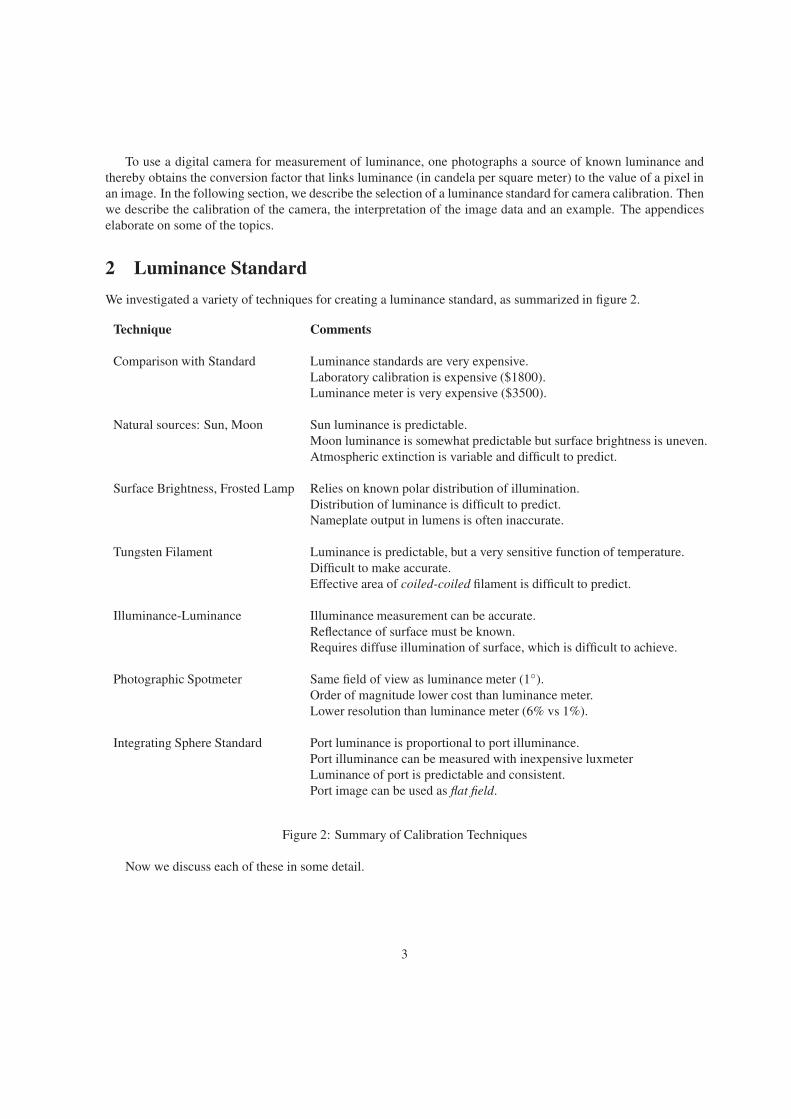
We investigated a variety of techniques for creating a luminance standard, as summarized in figure 2.

Technique Comments

Comparison with Standard Luminance standards are very expensive.

Laboratory calibration is expensive ($1800).

Luminance meter is very expensive ($3500).

Natural sources: Sun, Moon Sun luminance is predictable.

Moon luminance is somewhat predictable but surface brightness is uneven.

Atmospheric extinction is variable and difficult to predict.

Surface Brightness, Frosted Lamp Relies on known polar distribution of illumination.

Distribution of luminance is difficult to predict.

Nameplate output in lumens is often inaccurate.

Tungsten Filament Luminance is predictable, but a very sensitive function of temperature.

Difficult to make accurate.

Effective area of coiled-coiled filament is difficult to predict.

Illuminance-Luminance Illuminance measurement can be accurate.

Reflectance of surface must be known.

Requires diffuse illumination of surface, which is difficult to achieve.

Photographic Spotmeter Same field of view as luminance meter (1).

Order of magnitude lower cost than luminance meter.

Lower resolution than luminance meter (6% vs 1%).

Integrating Sphere Standard Port luminance is proportional to port illuminance.

Port illuminance can be measured with inexpensive luxmeter

Luminance of port is predictable and consistent.

Port image can be used as flat field.

Figure 2: Summary of Calibration Techniques

Now we discuss each of these in some detail.

3

Comparison with Standard

Professional caliber luminance meters and laboratory-calibrated luminance sources are far too expensive for gen-

eral purpose use by those working in light pollution abatement. For example, the new cost of a Minolta LS-100 is

$3500. The National Research Council of Canada quoted $1800 to calibrate a luminance meter2.

Natural Sources

Some natural sources (the sun, moon and stars) have a predictable luminance. The problem, as detailed in section

3.6, is atmospheric extinction, the attenuation of light in the atmosphere, which is not easily determined with

precision. The luminance of clear or overcast sky is variable over time and viewing angle [8].

A standard candle illuminates white paper at 1 ft-lambert (3.44 cd/m2) [5]. Unfortunately, readily available

candles have significant differences in light output and vary substantially over time [9].

Surface Brightness of Frosted Lamp

It is possible to relate the total output flux of a lamp (in lumens, specified on the package) to the brightness of

the surface of the lamp. For this to work, one must have an accurate map of the radiation pattern. This would

be straightforward if the lamp had a spherical radiation pattern, but that’s not usually the case. The luminance at

the top of the bulb, or at the side in line with the filament, is quite noticeably less than other areas of the bulb.

Furthermore, the nameplate flux may be significantly different than the actual flux.

Another approach is to measure the illuminance at some distance from the lamp and then calculate the lumi-

nance of the source. Again, that approach requires accurate knowledge of the radiation pattern.

The details and an example are in section 3.5.

Tungsten Filament

The luminance of the tungsten filament in an incandescent lamp is a predictable function of its temperature. The

filament temperature can be determined from its resistance, which in turn depend on the operating current and

voltage. In theory, this makes the basis a luminance standard [10].

This approach is attractive because the filament temperature can be related to the luminous output of the lamp,

which is a useful check on the calculations.

There are two complications. First, the luminance is a 9th power function of filament temperature. A 1%

error in temperature results in a 9% error in luminance. Consequently, the accuracy requirement for temperature

is very stringent. Second, the luminance may be affected by a light recycling effect resulting from the complex

coiled-coiled shape of the filament.

The tungsten filament is a small target. It does not fill the entire aperture of a luminance meter such as the

Tektronix J-16 with 6503 probe. This would require a correction factor, another possible source of error. On the

other hand, a digital camera could be used to record the luminance of a filament, assuming that the area of the

filament completely covers several pixels.

A tungsten filament could be useful as a luminance standard, but it needs to be verified by other methods.

Illuminance to Luminance

Under the right circumstances, the luminance L of a surface is related to the illuminance E and reflectance ρ by

equation 1.

2There are some bargains to be had. The author obtained a Tek J-16 Photometer with various measuring heads, including the J6503luminance probe, from eBay [6]. However, the unit required some repair work and the age of the unit (1985) suggested that the calibration

was not reliable.

4

L =Eρ

πcandela/meter2 (1)

where the quantities are

L Luminance emitted from the surface candela/meter2

E Illuminance of light falling on the surface lux

ρ Reflectance (dimensionless)

The device used to measure E – an illuminance meter or luxmeter – is readily available and inexpensive.

Determining the reflectance of a surface is a bit more complicated [11], [12], but it can be done. The grey card

popular in photography – readily available at low cost – has a known reflectance of 18% and can be used as a

standard for comparison.

The challenge in this method is properly illuminating the surface. It must be illuminated uniformly and equally

from all directions. In other words, the illuminating field must be diffuse. It turns out that this is very difficult to

achieve in a laboratory setting with conventional lighting sources. However, a diffuse field is achievable inside an

integrating sphere, as described below, and under those circumstances this becomes a practical technique.

Photographic Spotmeter

A photographic spotmeter is a narrow field of view exposure meter used in photography. The spotmeter is avail-

able from a number of manufacturers. We’ll focus on the Minolta Spotmeter F, which is similar in appearance to

the Minolta LS-100 luminance meter shown in figure 1(b) on page 2.

A photographic spotmeter displays exposure value [15]. The exposure value is the degree of exposure of the

camera film or sensor. Various combinations of aperture and shutter speed can be used to obtain the same exposure

value, according to equation 2.

2EV =N2

t(2)

where the quantities are:

EV Exposure Value

N Aperture number (F-Stop)

t Exposure time, seconds

It can also be shown [16] that scene luminance and exposure value are related according to equation 3.

2EV =Ls S

Km

(3)

where the quantities are:

EV Exposure Value, as before

S ISO setting (see section 3.7, page 18)

Ls Scene Luminance, candela/meter2

Km Calibration constant for the meter, equal to 14 for Minolta

Equation 3 provides us with a route to measuring luminance. Typically, the spotmeter displays EV units at an

assumed ISO of 100. A written table in the meter operating manual or software in the unit incorporates the meter

constant (14 for Minolta) and uses equation 3 to convert exposure value to luminance.

5

To get some idea of the advantages and limitations of a photographic spotmeter, it’s worthwhile to compare

the Minolta LS-100 luminance meter [17] and Minolta F photographic spotmeter [18].

Minolta LS-100 Luminance Meter Minolta F Spotmeter

Field of View 1 degree 1 degree

Range 0.001 to 300,000 cd/meter2 0.29 to 831,900 cd/meter2

Accuracy 2% 7%

Resolution 0.1% 6%

Price $3500.00 (New) $2500 (Used) $339.00 (Used)

The resolution and accuracy of the spotmeter are more than satisfactory for photographic use, but rather coarse

for for a precise measurement of luminance. That said, it may be useful to rent a photographic spotmeter for a

modest fee3, in order to do a sanity check on a luminance calibration source.

Because luminance is an exponential function of exposure value, it’s very sensitive to small changes in ex-

posure value. The limited resolution of the spotmeter means that there is significant uncertainty in a luminance

reading. For example, when the exposure value changes from 11 to 11.1, (1%) the luminance value changes by

7%.

Integrating Sphere

Figure 3: Light Integrating Sphere

The port of a light integrating sphere has a

luminance that is a simple function of illu-

minance. As shown in [13], the luminance

at the port is given by:

L =E

π(4)

Figure 3 shows the 14 inch diame-

ter light integrating sphere that was con-

structed for these measurements. Con-

struction and use of the sphere is described

in reference [13].

In operation, one measures the illumi-

nance of the light field exiting the port and

applies equation 4. (Notice the illuminance

meter to the left of the sphere in figure 3).

In figure 3, the Tektronix J-16 Photometer

with 6503 Luminance Probe is located at the sphere port to measure the luminance. One could then adjust the

luminance meter to display the calculated value of luminance.

The measurement is dependent on the sphere functioning correctly, that is, providing a uniform and diffuse

field of light. This is easy to confirm with measurements at the port.

• The accuracy of the method depends on the accuracy of the luxmeter. It is relatively inexpensive to have a

luxmeter calibrated, about $200 is quoted in advertisements [14].

• The port provides a large area of uniform illumination. It is a suitable target for luminance meter (because

it fills the entire measurement aperture) or as the flat field image for a digital camera.

3In Toronto, Vistek will rent a Minolta F spotmeter for $15 per day.

6

3 Camera Calibration

Luminance to Pixel Value

The digital camera turns an image into a two dimensional array of pixels. Ignoring the complication of colour,

each pixel has a value that represents the light intensity at that point.

The amount of exposure (the brightness in the final image) is proportional to the number of electrons that are

released by the photons of light impinging on the sensor4. Consequently, it’s proportional to the illuminance (in

lux) times the exposure time, so the brightness is in lux-seconds. Invoking the parameters of the camera, we have

in formula form [16]:

Nd = Kc

(

t S

fs2

)

Ls (5)

where the quantities are

Nd Digital number (value) of the pixel in the image

Kc Calibration constant for the camera

t Exposure time, seconds

fs Aperture number (f-stop)

S ISO Sensitivity of the film (section 3.7, page 18)

Ls Luminance of the scene, candela/meter2

The digital number (value) Nd of a pixel is determined from an analysis of the image, using a program like

ImageJ [19]. Pixel value is directly proportional to scene luminanceLs. It’s also dependent on the camera settings.

For example, if the luminance is constant while the exposure time or film speed are doubled, the pixel value

should also double. If the aperture number fs is increased one stop (a factor of 1.4), the area of the aperture is

reduced by half so the pixel value will also drop by half [20].

In theory, to calibrate the camera one photographs a known luminance, plugs values for luminance, exposure

time, film speed and aperture setting into equation 5, and calculates the calibration constant Kc.

It should then be possible to use the camera at other settings of exposure time, film speed and aperture setting.

One determines the pixel value in the image and then runs equation 5 in the other direction to calculate an unknown

luminance.

Maximum Pixel Value

The pixel values are represented inside the camera as binary numbers. The range for the pixel value Nd is from

zero to Nmax, where:

Nmax = 2B − 1 (6)

where B is the number of bits in the binary numbers. For example, for a 16 bit raw image, the range of values

is from zero to 216 − 1 = 65535. For an 8 bit JPEG image, the range of values is considerably smaller, from zero

to 28−1 = 255. In order not to lose information in the image the exposure must be adjusted so that the maximum

pixel value is not exceeded.

4Clark [7] calculates for the Canon D10 DSLR camera at ISO 400, that each digital count in a pixel value is equivalent to 28.3 photons.

7

Vignetting

(1/1000 sec) (1/100 sec)

F4.0

F5.0

F6.3

Ls: 499 candela/metre^2F: 5.0ISO: 200

0

5000

10000

15000

20000

25000

30000

35000

40000

45000

50000

0 2 4 6 8 10

Pixel Value

Exposure Time, mSec

(a) Pixel Value vs Exposure Time

8.0

5.6

4.5

2.8

3.2

3.5

4.0

5.0

7.16.3

Ls: 499 cd/metre^2t: 1/200 secISO: 200

0

10000

20000

30000

40000

50000

0 0.02 0.04 0.06 0.08 0.1 0.12 0.14

Pixel Value

1/Aperture^2

(b) Pixel Value vs Aperture

Ls: 499 candela/metre^2t: 1/800 secF: 5.0

0

2000

4000

6000

8000

10000

12000

14000

16000

18000

0 100 200 300 400 500 600 700 800 900ISO

Pixel Value

(c) Pixel Value vs ISO

Figure 4: Canon SX120IS Camera Calibration

The light transmission of the camera lens tends to decrease to-

ward the edges of the lens, an effect known as vignetting. The

effect can be quantified in equation form. However it is more

practical to photograph an image with uniform brightness (a

so-called flat field). Then use an image analysis program to

check pixel value near the centre and near the edge5 The exit

port of the integrating sphere used for these measurements is

a suitable flat field. It’s illumination has been measured with a

narrow field luminance meter and determined to be reasonably

uniform.

Image File Format: Raw, DNG, JPEG and TIFF

Image formats fall into two categories: raw (lossless) and

compressed (lossy).

A raw image file stores the pixel values exactly as they

are generated by the image sensor. Each camera manufacturer

uses a different raw format and image processing programs in

general cannot accept proprietary format files. Consequently,

it is usual to convert raw format to some more universal for-

mat, such as TIFF (tagged image file format). A TIFF format-

ted file can contain all the information of the original so it can

also be a lossless format6.

Raw and TIFF have the advantage that no information is

lost, but the files are very large. For example, a Canon raw

format (DNG) is typically about 15 MBytes per image. A

TIFF formatted file is larger, in the order of 60 MBytes per

image. These are colour images. If a TIFF file is processed to

monochrome (which is the case for luminance measurements),

then the file size drops to about 20MBytes per image.

It turns out that raw format images are overkill for many

applications. There is redundant information in most images

and with careful processing, the numerical representation of

each pixel value can be reduced from 16 bits to 8 bits. To a hu-

man observer, there is little or no difference between raw and

compressed versions of an image. Compressing an image is

lossy – the process cannot be reversed to reconstitute the orig-

inal raw image. However, the size is reduced tremendously

which saves on storage space and speeds up image transfer.

A typical JPEG-compressed image file is about 71 KBytes in

size, a factor of 800 smaller than the comparable TIFF image.

Compressed images permit many more images in a given

storage space and transfer more quickly between camera and

5In the case of the Canon SX-120IS point-and-shoot camera, it appears that vignetting is absent, possibly by compensation by the camera

computer.6The TIFF file format has the capability of using no compression, lossless compression and lossy compression. It’s frequently used in

lossless mode.

8

computer.

High end digital cameras such as digital single-lens reflex (DSLR) cameras can produce images in raw or

compressed (JPEG) format. Most point-and-shoot cameras can only produce compressed format7.

Image File Format and Luminance Measurement

A JPEG formatted image has a non-linear relationship between exposure value and pixel code. In calibrating a

camera for luminance measurement is necessary to determine this relationship and account for its effect under

conditions of different aperture, exposure interval, and ISO number. This greatly complicates the analysis.

A raw formatted image, on the other hand, uses equation 5 (page 5) directly. Image pixel value is directly or

inversely proportional to the camera parameters and the scene luminance. For example, a plot of pixel value vs

exposure interval is a straight line that passes through the origin.

In theory, both raw and compressed format images can be used for luminance measurement. Jacobs [22],

Gabele-Wuller [24], [4] used JPEG formatted images. Craine [23] and Flanders [27] used JPEG format images,

but restricted the exposure range to minimize the non-linearity of JPEG compression. Meyer [25] and Hollan [26]

used raw format.

Initially we worked with JPEG formatted images and then subsequently switched to raw format. Raw format

images simplified the process and generated results that were more predictable and consistent.

Settings and Measurements

In the ideal case, the camera calibration relationship (equation 5 on page 7) would apply exactly to the camera.

In that case, one measurement would be sufficient to determine the value of the calibration constant. One would

photograph some source of known luminance Ls, determine the equivalent value Nd of the pixels in the image,

and note the camera settings for ISO, exposure time and aperture. Plug these values into equation 5 and solve for

the calibration constant Kc.

For that approach to work, the settings for shutter speed, aperture and ISO must be reflected accurately in the

operation of the camera hardware.

Figure 4(a) shows this is the case for camera shutter speed, where pixel value increases linearly with exposure

time (inversely with shutter speed)8.

Figure 4(b) shows the relationship between pixel value and aperture. At large apertures, above F 4.0, the

relationship becomes non-linear. One would either avoid those aperture values or determine the specific value for

the calibration constant at each aperture.

Figure 4(c) shows the relationship between pixel value and ISO9. As expected, the digital number is a linear

function of the ISO over the range shown on the graph10.

With a large number of measurements in hand at various values of shutter speed, aperture and ISO, excluding

values where the relationship is non-linear, we used a spreadsheet to solve for the corresponding value of the

7Canon point-and-shoot cameras can be modified with the so-called CHDK software [21], which enables them to produce raw format

images. The Canon G15 and G15 point-and-shoot cameras can produce raw format images.8Debevec [28] has an interesting comment on shutter speed: Most modern SLR cameras have electronically controlled shutters which give

extremely accurate and reproducible exposure times. We tested our Canon EOS Elan camera by using a Macintosh to make digital audio

recordings of the shutter. By analyzing these recordings we were able to verify the accuracy of the exposure times to within a thousandth of a

second.

Conveniently, we determined that the actual exposure times varied by powers of two between stops ( 1/64, 1/32, 1/16, 1/8, 1/4, 1/2, 1, 2, 4,

8, 16, 32), rather than the rounded numbers displayed on the camera readout ( 1/60, 1/30, 1/15, 1/8, 1/4, 1/2, 1, 2, 4, 8, 15, 30).9ISO number is referred to as film speed in film cameras. In a digital camera, it is a function of the amplification applied to the pixel value

after capture.10This camera provides an additional ISO setting of 1600, but the increase in digital number for that ISO setting is not proportional at all,

which makes the setting unsuitable for luminance measurement. In light pollution work, the intensity of sources makes it unlikely that ISO

1600 would be useful. It could however be of interest to someone documenting sky glow, which is relatively faint.

9

camera constant Kc in equation 5. For the SX120IS camera, using 55 different combinations of settings we

measured a camera constant value Kc of 815 with an RMS deviation11 of 4.7%.

Magnification

(a) LED Array

(b) Image

(c) Profile Plot

Figure 5: Light Emitting Diode Array

Many sources of light pollution form a small camera image,

so it is very useful to be able to magnify the image using the

camera lens zoom function. The Canon SX120IS used in this

exercise has a zoom range of ×1 to ×10. The CHDK software

extends this to ×23. (Also helpful in the case of the Canon

SX120IS is the electronic image stabilization feature, which

allows one to take hand-held pictures at the maximum zoom

setting).

If the camera zoom lens setting is changed, does that have

an effect on the luminance measurement? At first thought

that would seem to be the case, since luminance is measured

in candela per square metre, and the area of observation has

changed. However, the luminous power in candela is mea-

sured in lumens per steradian (solid angle). A change of mag-

nification alters the area and solid angle such that the two ef-

fects cancel. In an ideal system, where there are no losses,

luminance is invariant [29], [30] .

We checked this by taking images of the integrating sphere

port from a distance of 6.25 meters, at zoom settings of ×1,

×10 and ×23. The average digital number in the image of the

illuminated sphere port was constant for the three images, to

within 2%.

This is very convenient, since the same camera calibration

constant applies regardless of the camera zoom lens setting.

4 Example Measurement: LED Array

We use the light emitting diode (LED) array of figure 5(a) to

illustrate the process of using a digital photograph to measure

the luminance of the individual LEDs. This cannot be done

easily using the Tek J-16 luminance meter or Minolta Spot-

meter M because their sensor field of view is much larger than

the light emitting source, and a measurement will underesti-

mate the luminance.

The array was photographed with the camera in Manual

mode to establish the shutter speed, aperture and ISO, keep-

ing an eye on the camera real-time histogram display to ensure

that the image was not overexposed. The camera CHDK soft-

ware generates two images, a Canon RAW format image and

11RMS: Root Mean Square. The deviation values are first squared. Then one takes the average of these squares. Finally, one takes the

square root of the average. The result is an indication of the typical value of a deviation, while ignoring the effect of the sign of the deviation.

10

a JPEG formatted image. The RAW format image was processed to monochrome TIFF format, as described in

Work flow, section 3.8, page 18.

An image of the illuminated array is shown in figure 5(b). The TIFF version of the image was analysed in

ImageJ. A profile line was drawn through three of the LEDs to determine the corresponding pixel values, using

the profile analysis tool. The resultant plot is shown in figure 5(c).

The EXIF file from the JPEG image was used to confirm the camera settings. The camera constant was deter-

mined earlier, page 10. The image information is summarized as follows:

Quantity Symbol Value

Maximum Pixel Value Nd 64197

Shutter Speed t 1/2500 sec

Aperture (F-Stop) fs 8.0

ISO Setting S 80

Camera Constant Kc 815

Rearranging equation 5 (page 7) to solve for luminance, we have:

Ls =Nd f

2

s

Kc t S

=64197× 8.02

815×1

2500× 80

= 157, 538 candela/metre2

According to the table of luminances in section 3.1 (page 12), 50,000 candela/metre2 is Maximum Visual

Tolerance. This makes the unshielded LED array a potential source of glare.

Extending Luminance Range

The pixel value in the previous example is very close to the allowable maximum, 65536 (216). The camera settings

are at their limit (fastest shutter speed, minimum aperture, minimum ISO) for the camera to minimize exposure.

Is it possible to photograph images of greater luminance?

There are two possible solutions.

• The CHDK software on a Canon point-and-shoot camera supports custom exposure settings up to 1/100k

seconds [31], [32], so you could increase the shutter speed (ie, decrease the shutter interval). CHDK also

supports custom ISO values, starting at 1, so you could reduce the ISO setting.

In general, these options are not available to unmodified DSLR (digital single-lens reflex) cameras.

• A neutral density filter can reduce the luminance of the image. For example, an ND4 filter reduces the

luminance by a factor of 4. Neutral density filters are readily available for DSLR cameras.

Both methods should be calibrated. With an inexpensive set of neutral density filters we found that the actual

attenuation was as much as 30% different from the labeled value.

11

5 Appendices

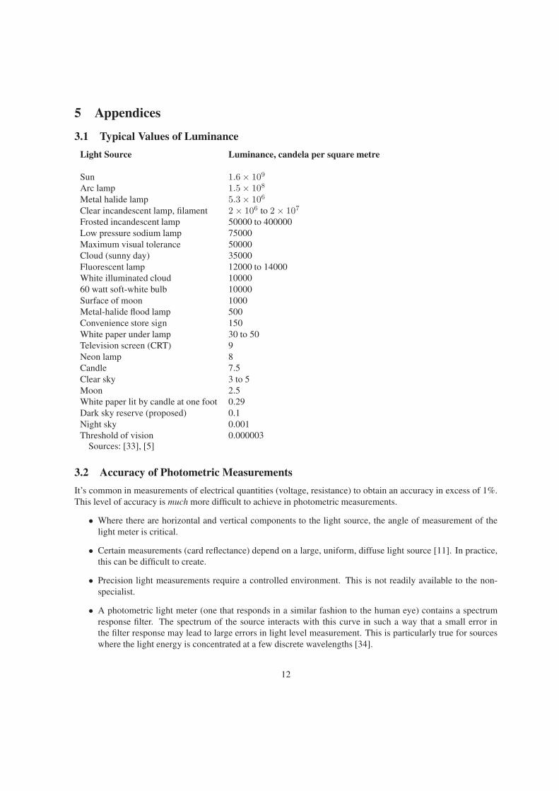
3.1 Typical Values of Luminance

Light Source Luminance, candela per square metre

Sun 1.6× 109

Arc lamp 1.5× 108

Metal halide lamp 5.3× 106

Clear incandescent lamp, filament 2× 106 to 2× 107

Frosted incandescent lamp 50000 to 400000

Low pressure sodium lamp 75000

Maximum visual tolerance 50000

Cloud (sunny day) 35000

Fluorescent lamp 12000 to 14000

White illuminated cloud 10000

60 watt soft-white bulb 10000

Surface of moon 1000

Metal-halide flood lamp 500

Convenience store sign 150

White paper under lamp 30 to 50

Television screen (CRT) 9

Neon lamp 8

Candle 7.5

Clear sky 3 to 5

Moon 2.5

White paper lit by candle at one foot 0.29

Dark sky reserve (proposed) 0.1

Night sky 0.001

Threshold of vision 0.000003Sources: [33], [5]

3.2 Accuracy of Photometric Measurements

It’s common in measurements of electrical quantities (voltage, resistance) to obtain an accuracy in excess of 1%.

This level of accuracy is much more difficult to achieve in photometric measurements.

• Where there are horizontal and vertical components to the light source, the angle of measurement of the

light meter is critical.

• Certain measurements (card reflectance) depend on a large, uniform, diffuse light source [11]. In practice,

this can be difficult to create.

• Precision light measurements require a controlled environment. This is not readily available to the non-

specialist.

• A photometric light meter (one that responds in a similar fashion to the human eye) contains a spectrum

response filter. The spectrum of the source interacts with this curve in such a way that a small error in

the filter response may lead to large errors in light level measurement. This is particularly true for sources

where the light energy is concentrated at a few discrete wavelengths [34].

12

The specified and measured accuracies of four illuminance meters is shown in section 3.4 on page 14. With

specified accuracies in the order of 5% and measured deviations from the average value in the order of 7%, an

overall measurement accuracy of 10% is reasonably achievable12.

Fortunately, the variability of light level measurements is mitigated to some extent by the non-linear response

of the human eye to different light levels, as we document in section 3.3. For example, a 25% change in brightness

is just detectable by the human vision system.

3.3 Perception of Brightness by the Human Vision System

According to Steven’s Law [36], brightness increases as a 0.33 power of the luminance13. In formula form:

S = K L0.33 (7)

where S is the perceived brightness (the sensation), K is a constant and L is the luminance.

Since the exponent is less than unity, the equation has the effect of reducing errors in luminance measurement.

We illustrate this with an example.

Example

Suppose that a luminance measurement is in error by +10%. What is the brightness perception of that error?

Solution

Call the correct sensation and luminance S and L. Call the measured sensation and luminance Sm and Lm.

Define the ratio R: Lm = R L.

Then from equation 7 we have:

S = K L 0.33Sm = K Lm0.33 = K (RL) 0.33 = K R 0.33L 0.33

Now find the ratio of the measured and true sensation:

Sm

S=

K R 0.33L 0.33

KL 0.33= R 0.33

The measured luminance is 10% larger than the actual luminance, so R = 1.10.

Then:

Sm

S= R 0.33 = 1.10 0.33 = 1.03

That is, the perception of the brightness is only 3% high when the actual luminance is 10% high.

The just noticeable difference for brightness is 7.9%, [37] so the 3% difference would be undetectable.

Using equation 7, one can show that a just noticeable change in brightness requires a luminance increase of

25%. A perceived doubling of brightness requires a luminance increase of approximately 8 times (800%).

12It may be possible to check the calibration of an illuminance meter by measuring the horizontal illuminance from the sun at noon. A table

of solar illuminance for various elevations of the sun above the horizon is in reference [35].13This greatly simplifies a complex situation. The perception of brightness is strongly determined by the size of the source and its surround-

ings. However, it illustrates the concept and is roughly true for a small source against a dark background.

13

3.4 Comparing Illuminance Meters

To determine the relative consistency of illuminance readings, the readings of four illuminance meters. The meter

sensor was placed in exactly the same position each time, and care taken not to shadow the sensor.

Meter Range Accuracy Reference

Tek J10 with J6511 Probe 0.01 to 19,990 lux ±5% [38]

Amprobe LM-80 0.01 to 20,000 lux ±3% [39]

Mastech LX1330B 1 to 200,000 lux ±3% ±10 digits [40]

Extech 401025 1 to 50,000 lux ±5% [41]

The measurement results are shown in figure 6.

10

100

1000

10 100 1000

Mea

sure

d

Average

Tek J16 with J6511 ProbeAmprobe LM−80

Mastech LX1330BExtech 401025

Figure 6: Four Illuminance Meters: Tek J10 with J6511 Probe, Amprobe LM-80, Mastech LX1330B, Extech

401025

The measured RMS deviations from the average were:

Meter RMS Deviation from Average

Tek J10 with J6511 Probe 6.9%

Amprobe LM-80 6.4%

Mastech LX1330B 8.1%

Extech 401025 12.4%

On the basis of the specified accuracy and measured deviation from average, an overall measurement accuracy

of ±10% is a reasonable goal.

14

3.5 Frosted Incandescent Lamp Calibration

Luminance from Total Output Flux

Knowing the total light output in lumens of a frosted incandescent lamp on can in theory determine the surface

brightness of the lamp. We can predict surface luminance as follows:

1. Total luminous flux Φ in lumens is known from the label on the box.

2. The bulb radiates through some solid angle Ω steradians.

3. Then the luminous intensity I is given by

I =Φ

ΩCandela (8)

4. The luminance of the bulb is equal to the luminous intensity I Candela divided by the surface area of the

bulb Ab meters2.

L =I

Ab

Candela/meters2 (9)

Example: Surface Luminance from Nameplate Output

The Sylvania DoubleLife 60 watt lamp has a total output of 770 lumens. The bulb diameter is 6cm. What is the

luminance of the bulb surface?

Solution

1. The total flux output is:

Φ = 770 lumens

2. Assume that the radiating pattern is a sphere, with 13% removed to account for the base. Then the radiating

angle Ω is:

Ω = 4× π × (1− 0.13) = 10.92 steradians

3. The luminous intensity I is given by equation 8 above:

I =Φ

Ω=

770

10.92= 70.51 candela

4. The surface area of the bulb Ab is approximately a sphere of radius r = 3 centimeters:

Ab = 4πr2 = 4× π ×

(

3

100

)2

= 0.0113 meters2

The luminance is the luminous intensity I divided by the bulb surface area Ab (equation 9 above).

L =I

Ab

=70.51

0.0113= 6240 candela/meters2

15

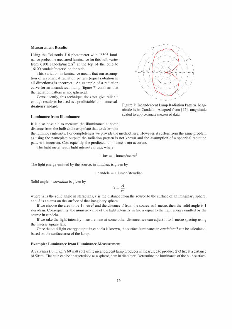
Measurement Results

40 206080100

Figure 7: Incandescent Lamp Radiation Pattern. Mag-

nitude is in Candela. Adapted from [42], magnitude

scaled to approximate measured data.

Using the Tektronix J16 photometer with J6503 lumi-

nance probe, the measured luminance for this bulb varies

from 6100 candela/meters2 at the top of the bulb to

16100 candela/meters2 on the side.

This variation in luminance means that our assump-

tion of a spherical radiation pattern (equal radiation in

all directions) is incorrect. An example of a radiation

curve for an incandescent lamp (figure 7) confirms that

the radiation pattern is not spherical.

Consequently, this technique does not give reliable

enough results to be used as a predictable luminance cal-

ibration standard.

Luminance from Illuminance

It is also possible to measure the illuminance at some

distance from the bulb and extrapolate that to determine

the luminous intensity. For completeness we provide the method here. However, it suffers from the same problem

as using the nameplate output: the radiation pattern is not known and the assumption of a spherical radiation

pattern is incorrect. Consequently, the predicted luminance is not accurate.

The light meter reads light intensity in lux, where

1 lux = 1 lumen/metre2

The light energy emitted by the source, in candela, is given by

1 candela = 1 lumen/steradian

Solid angle in steradian is given by

Ω =A

r2

where Ω is the solid angle in steradians, r is the distance from the source to the surface of an imaginary sphere,

and A is an area on the surface of that imaginary sphere.

If we choose the area to be 1 metre2 and the distance d from the source as 1 metre, then the solid angle is 1

steradian. Consequently, the numeric value of the light intensity in lux is equal to the light energy emitted by the

source in candela.

If we take the light intensity measurement at some other distance, we can adjust it to 1 metre spacing using

the inverse square law.

Once the total light energy output in candela is known, the surface luminance in candela/m2 can be calculated,

based on the surface area of the lamp.

Example: Luminance from Illuminance Measurement

A Sylvania DoubleLife 60 watt soft white incandescent lamp produces is measured to produce 273 lux at a distance

of 50cm. The bulb can be characterised as a sphere, 6cm in diameter. Determine the luminance of the bulb surface.

16

Solution

1. Adjust the reading in lux to a distance of 1 metre:

E1

E2

=

(

l2l1

)2

E2 = E1

(

l1l2

)2

= 273×

(

0.5

1.0

)2

= 68.25 lux, or lumens/m2

2. This is at a distance of 1 metre, so the source is emitting total energy of the same amount, 68.25 candela

(lumen/steradian).

3. The surface area of a sphere is given by S = 4πr2, where r is the physical radius of the lamp, 3 centimeters.

S = 4πr2 = 4× 3.14×

(

3

100

)2

= 0.0113 meters2

4. Now we can calculate the luminance in candela/metre2.

L =C

S=

68.25

0.0113= 6039 candela/m2

Light level measurements of the incandescent lamp should be taken under the following conditions:

• Other light sources should be turned off or it should be established that they are dim enough that they do

not materially affect the measurement.

• The light source and meter should be arranged so that the direct light from the lamp predominates. That

requires reflecting surfaces to be as far away as possible and if necessary cloaked with light absorbing

material.

• Ryer [43] suggests setting up an optical bench with a series of baffles. Each baffle is a black opaque sheet

mounted at right angles to the optical path. A hole in each baffle is centred on the optical path. This prevents

stray light, from a similar direction as the source, from reaching the detector.

• There is a 20% decrease in light output from the side of an incandescent lamp to the top. Consequently,

whatever orientation is used for the measurement of light level should also be used for luminance.

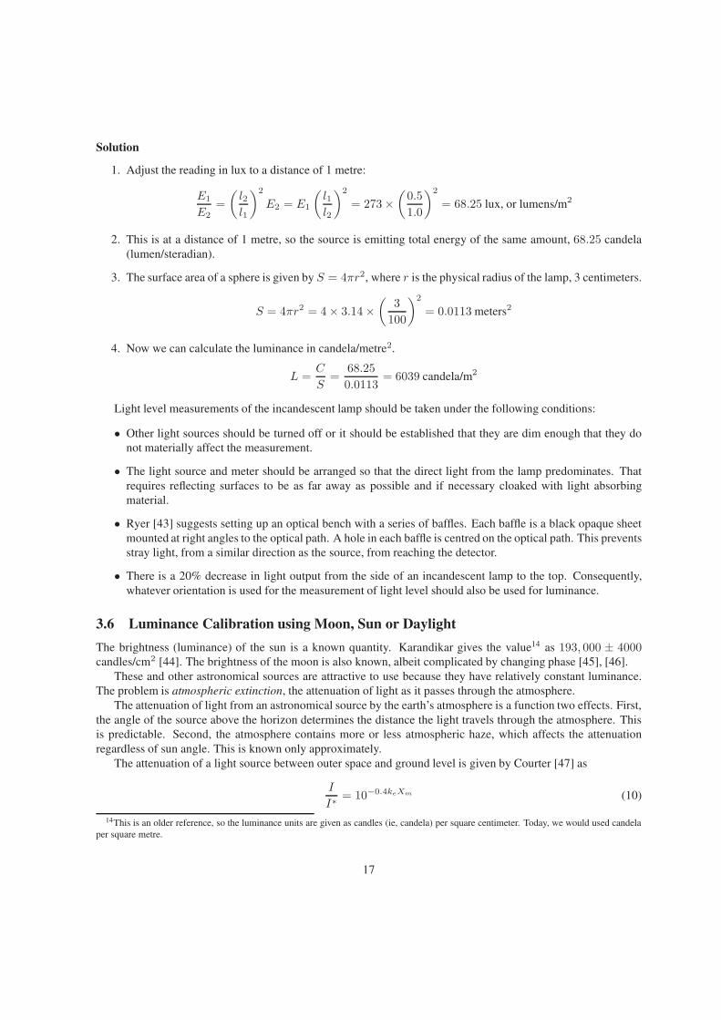
3.6 Luminance Calibration using Moon, Sun or Daylight

The brightness (luminance) of the sun is a known quantity. Karandikar gives the value14 as 193, 000 ± 4000candles/cm2 [44]. The brightness of the moon is also known, albeit complicated by changing phase [45], [46].

These and other astronomical sources are attractive to use because they have relatively constant luminance.

The problem is atmospheric extinction, the attenuation of light as it passes through the atmosphere.

The attenuation of light from an astronomical source by the earth’s atmosphere is a function two effects. First,

the angle of the source above the horizon determines the distance the light travels through the atmosphere. This

is predictable. Second, the atmosphere contains more or less atmospheric haze, which affects the attenuation

regardless of sun angle. This is known only approximately.

The attenuation of a light source between outer space and ground level is given by Courter [47] as

I

I∗= 10−0.4keXm (10)

14This is an older reference, so the luminance units are given as candles (ie, candela) per square centimeter. Today, we would used candela

per square metre.

17

where

I Intensity at the base of the atmosphere

I∗ Intensity at the top of the atmosphere

ke Extinction coefficient, depending on clarity of the atmosphere, typically 0.20 to 0.27, ex-

treme values 0.11 to 0.7

Xm Air Mass, equal to 1/ cos(θ), where θ is the angle between the zenith and the sun angle,

67 in this case.Unfortunately, there is no straightforward way to determine the extinction coefficient ke. A variation of 0.11 to

0.7 would a variation from 0.88 to 0.46 in the ratio of extraterrestrial to terrestial luminance, which is unacceptably

large.

3.7 ISO Speed Rating

In a film camera, the sensitivity of the film (film speed) is specified by a so-called ISO number. A faster film (one

with a higher ISO number) is more sensitive to light [48]. The commonly used ISO scale for film speed increases

in a multiplicative fashion, where the factor is approximately 1.2 between steps15.

In a digital camera, the ISO number refers to the sensitivity of the image sensor, specifically referred to as

the ISO Speed Rating. To change the sensitivity of a film camera, one needs to purchase and install a different

film. In a digital camera, the operator (or the automatic exposure mechanism) can set the ISO Speed Rating to a

different value16.

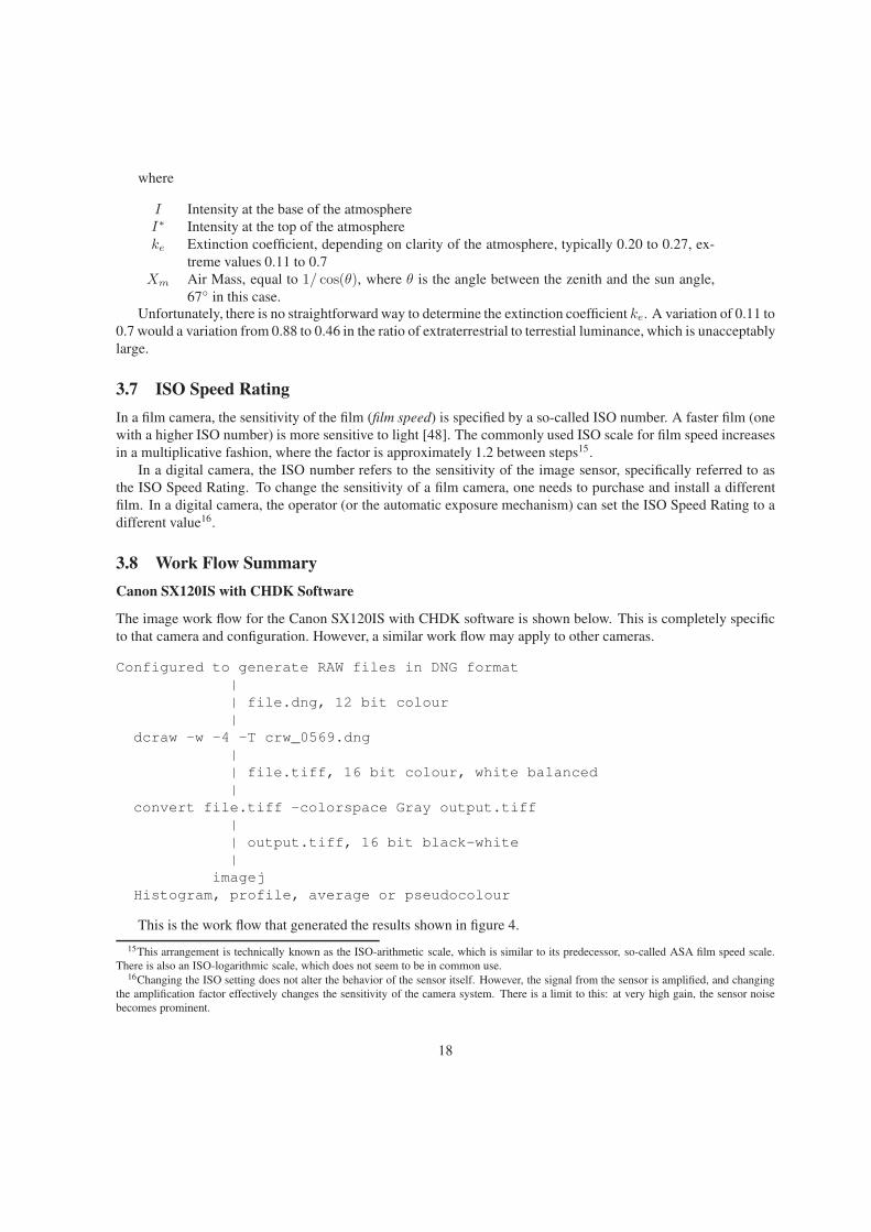
3.8 Work Flow Summary

Canon SX120IS with CHDK Software

The image work flow for the Canon SX120IS with CHDK software is shown below. This is completely specific

to that camera and configuration. However, a similar work flow may apply to other cameras.

Configured to generate RAW files in DNG format

|

| file.dng, 12 bit colour

|

dcraw -w -4 -T crw_0569.dng

|

| file.tiff, 16 bit colour, white balanced

|

convert file.tiff -colorspace Gray output.tiff

|

| output.tiff, 16 bit black-white

|

imagej

Histogram, profile, average or pseudocolour

This is the work flow that generated the results shown in figure 4.

15This arrangement is technically known as the ISO-arithmetic scale, which is similar to its predecessor, so-called ASA film speed scale.

There is also an ISO-logarithmic scale, which does not seem to be in common use.16Changing the ISO setting does not alter the behavior of the sensor itself. However, the signal from the sensor is amplified, and changing

the amplification factor effectively changes the sensitivity of the camera system. There is a limit to this: at very high gain, the sensor noise

becomes prominent.

18

Canon G15, G16

For these cameras we used a simplified workflow. As shown in Konnik [56], the Canon raw file in CR2 format

may be processed to a linear, 16 bit TIFF format file in one step, using the DCRaw command:

dcraw -4 -T -D -v file.CR2

-4 Output 16 bit linear file without brightening

-T Output file format TIFF

-D Document Mode

-v Verbose output

Using this DCRaw command on Canon CR2 format files, we found a maximum value of 4095 (212 − 1),

which implies 12 bit A/D conversion in the camera. The average minimum value (black level offset), obtained in

a dark frame, was 127 (27 − 1).

3.9 Using ImageJ To Determine Pixel Value

1. Start ImageJ.

2. Open the raw image file (eg, output_0569.tiff).

3. If the image needs to be scaled, place the cursor in the image and hit either the + or − key to scale the

image. This has no effect on the maximum, minimum or average value of the pixels, it just spreads out the

image, which may make it easier to work with.

4. Select the area of interest for example with the ellipse tool.

5. Under Analyse -> Set Measurements select the measurements required (eg, average grey scale).

6. Select Analyse -> Measure. A measurement window pops up or, if the measurements window is

already open, adds a line with the measurement of the average pixel value.

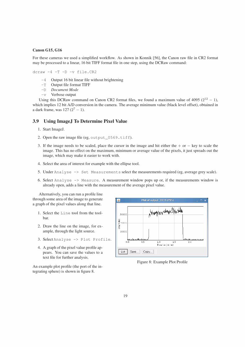
Figure 8: Example Plot Profile

Alternatively, you can run a profile line

through some area of the image to generate

a graph of the pixel values along that line.

1. Select the Line tool from the tool-

bar.

2. Draw the line on the image, for ex-

ample, through the light source.

3. SelectAnalyse -> Plot Profile.

4. A graph of the pixel value profile ap-

pears. You can save the values to a

text file for further analysis.

An example plot profile (the port of the in-

tegrating sphere) is shown in figure 8.

19

3.10 Using ImageJ To Generate a Luminance-Encoded Image

It is possible to use ImageJ to create a pseudo-coloured image, in which colours represent different levels of

luminance. This is particularly useful in assessing the illumination for architectural applications. To create a

pseudocolour image:

1. Open an image, which can be uncompressed TIFF format.

2. ChooseImage -> Colour -> Show LUT. The image is then pseudo-coloured using the default lookup

table (LUT), which is 0 to 255 grey levels. Notice that even though the image may have 216 (65536) levels

or whatever, the pseudocolour has only 28 (256). But that should be lots for the human observer.

3. Select Image -> Lookup Tables to select the 8 bit pseudocolour scheme. For example, the 16

colours lookup table shows sixteen different colours corresponding to equal parts of the 8 bit pixel range

0 to 255.

4. Select Image -> Color -> Show LUT to see a graphical representation of the lookup table, which

may then be extrapolated to 16 bit pixel value and then to luminance value.

5. Select Image -> Colour -> Edit LUT to see a widget containing 256 colour boxes, each corre-

sponding to a level in the image, that one can edit to modify the LUT.

3.11 Field of View of Digital Camera

The resolution of a digital camera is much higher than a luminance meter or photographic spotmeter. For example,

here is the calculation of resolution for the Canon G15 digital camera.

The pixel pitch P of the Canon G15 is given as 1.8µM. The focal length F at the wide angle setting is 6.1mm.

The ratio of these two is the viewing angle of one pixel, in radians.

θ =P

F=

1.8× 10−6

6.1× 10−3= 296× 10−6 radians

Convert this to degrees:

θ = 295× 10−6 radians ×180 degrees

π radians= 0.017 degrees

In the telephoto setting of the camera lens, the focal length is 30.5 mm and the corresponding field of view

0.0034 degrees.

Both these are a much narrower field of view than the 1 field of view of a luminance meter or photographic

spotmeter.

3.12 EXIF Data

EXIF data (also known as metadata) is information that is attached to an image. It contains photo parameters such

as exposure interval, aperture and ISO speed rating that is required in automating the conversion of image data to

luminance. This is enormously convenient in practice. It enables one to collect a series of images without having

to manually record the camera settings. One can return to images after the fact and determine settings from the

EXIF data.

From [49]:

20

Exchangeable image file format (EXIF) is a specification for the image file format used by digital

cameras. The specification uses the existing JPEG, TIFF Rev. 6.0, and RIFF WAV file formats, with

the addition of specific metadata tags. It is not supported in JPEG 2000, PNG, or GIF.

On a Linux system, the main EXIF data is obtained in the Gnome Nautilus file viewer by clicking on

Properties -> Image. The information may be copied and pasted into another document using the standard

copy and paste function.

On a Windows system, the EXIF data is obtained by right clicking on a photograph and selecting ’properties’.

The information cannot be copied and pasted.

A more complete listing of EXIF data is found using the command line program exiftool [50]. For

example, the command exiftool myfile.jpg lists the EXIF data for myfile.jpg.

EXIF data for the Canon SX120IS is shown below. The EXIF data for this camera is very extensive. For other

point-and-shoot cameras the data file is greatly abbreviated.

For legibility the EXIF data has been formatted slightly into different sections.

Image Description

Manufacturer Canon

Model Canon PowerShot SX120 IS

Orientation top - left

x-Resolution 180.00

y-Resolution 180.00

Resolution Unit Inch

Date and Time 2009:12:15 20:48:28

YCbCr Positioning co-sited

Thumbnail Directory

Compression JPEG compression

x-Resolution 180.00

y-Resolution 180.00


Exif Directory

Exposure Time 1/15 sec.

FNumber f/2.8

ISO Speed Ratings 640

Exif Version Exif Version 2.21

Date and Time (original) 2009:12:15 20:48:28

Date and Time (digitized) 2009:12:15 20:48:28

Components Configuration Y Cb Cr -

Compressed Bits per Pixel 3.00

Shutter speed 3.91 EV (APEX: 3, 1/14 sec.)

Aperture 2.97 EV (f/2.8)

Exposure Bias 0.00 EV

MaxApertureValue 2.97 EV (f/2.8)

Metering Mode Pattern

Flash Flash fired, auto mode,

red-eye reduction mode.

Focal Length 6.0 mm

Maker Note 2266 bytes unknown data

User Comment

FlashPixVersion FlashPix Version 1.0

Color Space sRGB

PixelXDimension 3648

PixelYDimension 2736

Focal Plane x-Resolution 16141.59

Focal Plane y-Resolution 16094.12

Focal Plane Resolution Unit Inch

Sensing Method One-chip color area sensor

File Source DSC

Custom Rendered Normal process

Exposure Mode Auto exposure

White Balance Auto white balance

Digital Zoom Ratio 1.00

Scene Capture Type StandardInterOperability Directory

21

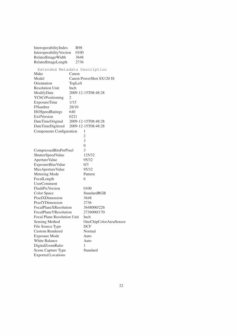
InteroperabilityIndex R98

InteroperabilityVersion 0100

RelatedImageWidth 3648

RelatedImageLength 2736

Extended Metadata Description

Make Canon

Model Canon PowerShot SX120 IS

Orientation TopLeft


ModifyDate 2009-12-15T08:48:28

YCbCrPositioning 2

ExposureTime 1/15

FNumber 28/10

ISOSpeedRatings 640

ExifVersion 0221

DateTimeOriginal 2009-12-15T08:48:28

DateTimeDigitized 2009-12-15T08:48:28

Components Configuration 1

2

3

0

CompressedBitsPerPixel 3

ShutterSpeedValue 125/32

ApertureValue 95/32

ExposureBiasValue 0/3

MaxApertureValue 95/32

Metering Mode Pattern

FocalLength 6

UserComment

FlashPixVersion 0100

Color Space StandardRGB

PixelXDimension 3648

PixelYDimension 2736

FocalPlaneXResolution 3648000/226

FocalPlaneYResolution 2736000/170

Focal Plane Resolution Unit Inch

Sensing Method OneChipColorAreaSensor

File Source Type DCF

Custom Rendered Normal

Exposure Mode Auto

White Balance Auto

DigitalZoomRatio 1

Scene Capture Type Standard

Exported Locations

22

References

[1] Measuring Light

Peter Hiscocks, December 6 2009

http://www.ee.ryerson.ca/˜phiscock/

[2] Mastech LX1330B Luxmeter

http://www.multimeterwarehouse.com/luxmeter.htm

[3] Minolta LS-100 Luminance Meter

http://www.konicaminolta.com/instruments/products/light/

luminance-meter/ls100-ls110/index.html

[4] The usage of digital cameras as luminance meters

Dietmar Wuller, Helke Gabele

Image Engineering, Augustinusstrasse 9d, 50226 Frechen, Germany

http://www.framos.eu/uploads/media/The_usage_of_digital_cameras_as_

luminance_meters_EI_2007_6502_01.pdf

[5] J16 Digital Photometer Instruction Manual

Tektronix Inc.

Nov 1986

[6] Tektronix J16 Digital Photometer Radiometer

http://www.testequipmentconnection.com/specs/TEKTRONIX_J16.PDF

[7] Digital Cameras: Counting Photons, Photometry, and Quantum Efficiency

http://www.clarkvision.com/imagedetail/digital.photons.and.qe/

[8] Sky Luminance Data Measurements for Hong Kong

C.S.Lau, Dr. D.H.W.Li

http://www.sgs.cityu.edu.hk/download/studentwork/bc-cl.pdf

[9] On the Brightness of Candles

Peter D. Hiscocks, April 2011


[10] Luminance of a Tungsten Filament

Peter D. Hiscocks, April 2011


[11] Issues in Reflectance Measurement

David L B Jupp

CSIRO Earth Observation Centre

Discussion Draft August 1996, updated April 1996

http://www.eoc.csiro.au/millwshop/ref_cal.pdf

[12] Measuring Reflectance

Peter D. Hiscocks, August 2011


23

[13] Integrating Sphere for Luminance Calibration

Peter D. Hiscocks, August 2011


[14] International Light Technologies: Custom Calibration for NON ILT Lux Meters http://www.

intl-lighttech.com/services/calibration-services

[15] Exposure Value

Wikipedia

http://en.wikipedia.org/wiki/Exposure_value

[16] Exposure Metering: Relating Subject Lighting to Film Exposure

Jeff Conrad

http://www.largeformatphotography.info/articles/conrad-meter-cal.pdf

[17] Specification, Minolta LS-100 Luminance Meter

Minolta

http://www.konicaminolta.com/instruments/products/light/

luminance-meter/ls100-ls110/specifications.html

[18] Specification, Minolta M Spotmeter

http://www.cameramanuals.org/flashes_meters/minolta_spotmeter_m.pdf

[19] ImageJ

Wayne Rasband

http://rsbweb.nih.gov/ij/

[20] F-Number

Wikipedia

http://en.wikipedia.org/wiki/F-number

[21] Installing CHDK on the Canon SX120IS Camera

Peter D. Hiscocks, October 2010


[22] High Dynamic Range Imaging and its Application in Building Research

Axel Jacobs

Advances in Building Energy Research, 2007, Volume 01

www.learn.londonmet.ac.uk/about/doc/jacobs_aber2007.pdf

[23] Experiments Using Digital Camera to Measure Commercial Light Sources

Erin M. Craine

International Dark-Sky Association

docs.darksky.org/Reports/GlareMetricExperimentWriteUpFinal.pdf

[24] The usage of digital cameras as luminance meters: Diploma Thesis

Helke Gabele

Faculty of Information, Media and Electrical Engineering

University of Applied Sciences Cologne, 2006

http://www.image-engineering.de/images/pdf/diploma_thesis/digital_

cameras_luminance_meters.pdf

24

[25] Development and Validation of a Luminance Camera

Jason E. Meyer, Ronald B. Gibbons, Christopher J. Edwards

Final Report, Virginia Tech Transportation Institute, 2009

http://scholar.lib.vt.edu/VTTI/reports/Luminance_Camera_021109.pdf

[26] RGB Radiometry by digital cameras

Jan Hollan

http://amper.ped.muni.cz/light/luminance/english/rgbr.pdf

[27] Measuring Skyglow with Digital Cameras

Tony Flanders

Sky and Telescope Magazine, February 2006

http://www.skyandtelescope.com/observing/home/116148384.html

[28] Recovering High Dynamic Range Radiance Maps from Photographs

Paul E. Debevec and Jitendra Malik

http://www.debevec.org/Research/HDR/debevec-siggraph97.pdf

[29] Jack O’Lanterns and integrating spheres: Halloween physics

Lorne A. Whitehead and Michele A. Mossman

American Journal of Physics 74 (6), June 2006, pp 537-541

[30] Wikipedia Talk: Luminance

Srleffler

http://en.wikipedia.org/wiki/Talk%3ALuminance

[31] CHDK Extra Features For Canon Powershot Cameras, User Quick Start Guide

http://images1.wikia.nocookie.net/__cb20100820031922/chdk/images/3/33/

CHDK_UserGuide_April_2009_A4.pdf

[32] Samples: High-Speed Shutter & Flash-Sync

http://chdk.wikia.com/wiki/Samples:_High-Speed_Shutter_%26_Flash-Sync

[33] Technical basics of light

OSRAM GmbH, 2010

http://www.osram.com/osram_com/Lighting_Design/About_Light/Light_%26_

Space/Technical_basics_of_light__/Quantitatives/index.html

[34] Photometric Errors with Compact Fluorescent Sources

M.J. Ouellette

National Research Council Report NRCC 33982

http://www.nrc-cnrc.gc.ca/obj/irc/doc/pubs/nrcc33982/nrcc33982.pdf

[35] Radiometry and photometry in astronomy

Paul Schlyter, 2009

http://stjarnhimlen.se/comp/radfaq.html

[36] Stevens’ power law

Wikipedia

http://en.wikipedia.org/wiki/Stevens%27_power_law

[37] Just Noticeable Difference

http://psychology.jrank.org/pages/353/Just-Noticeable-Difference.html

25

[38] Specification, Tektronix J6501 illuminance meter

http://www.testwall.com/datasheets/TEKTRJ6501.pdf

[39] Specification, Amprobe LM-80 illuminance meter

http://www.testequipmentdepot.com/amprobe/pdf/LM80.pdf

[40] Specification, Mastech LX1330B illuminance meter

http://www.multimeterwarehouse.com/LX1330B.htm

[41] Specification, Extech 401025 illuminance meter

http://www.extech.com/instruments/resources/datasheets/401025.pdf

[42] A Comparative Candelpower Distribution Analysis for Compact Fluorescent Table Lamp Systems

LBL-37010, Preprint L-195

Erik Page, Chad Praul and Michael Siminovich

University of Berkeley, California

btech.lbl.gov/papers/37010.pdf

[43] The Light Measurement Handbook

Alex Ryer

International Light, 1997

www.intel-lighttech.com

[44] Luminance of the Sun

R. V. Karandikar

Journal of the Optical Society of America

Vol. 45, Issue 6, pp. 483-488 (1955)

[45] The Moon’s Phase

Brian Casey

http://www.briancasey.org/artifacts/astro/moon.cgi

[46] Solar System Dynamics, Horizons Web Interface

Jet Propulson Laboratory

http://ssd.jpl.nasa.gov/horizons.cgi#results

[47] Correcting Incident Light Predictions for Atmospheric Attenuation Effects

Kit Courter, December 21, 2003

http://home.earthlink.net/˜kitathome/LunarLight/moonlight_gallery/

technique/attenuation.htm

[48] Film speed

Wikipedia

http://en.wikipedia.org/wiki/Film_speed

[49] Exchangeable image file format

Wikipedia

http://en.wikipedia.org/wiki/Exchangeable_image_file_format

[50] ExifTool

Phil Harvey

www.sno.phy.queensu.ca/˜phil/exiftool/

26

[51] Using a camera as a lux meter

Tim Padfield, May 1997

www.natmus.dk/cons/tp/lightmtr/luxmtr1.htm

[52] WebHDR

Axel Jacobs

https://luminance.londonmet.ac.uk/webhdr/about.shtml

Website for processing images into high dynamic range image and luminance map.

[53] DCRAW

http://en.wikipedia.org/wiki/Dcraw

[54] Luminance Measurement by Photographic Photometry

I.Lewen, W.B.Bell

Illuminating Engineering, November 1968, pp 582-589

http://www.ies.org/PDF/100Papers/063.pdf

[55] Measuring Camera Shutter Speed

Peter D. Hiscocks, May 2010

www.syscompdesign.com/assets/Images/AppNotes/shutter-cal.pdf

[56] Increasing Linear Dynamic Range of Commercial Digital Photocamera Used in Imaging Systems with Op-

tical Coding

M. Konnik, E.A.Manykin, S.N. Starikov

arXiv:0805.2690v1 [cs.CV] 17 May 2008

http://arxiv.org/pdf/0805.2690.pdf

[57] Derivation of the relationship between illuminance E and luminance L for a Lambertian reflective surface,

L = Eρ/π.

Yi Chun Huang

http://www.yichunhuang.com/files/teaching/landa/lambertian_luminance.pdf

[58] Measuring Luminance with a Digital Camera: Case History

Peter D. Hiscocks, December, 2013


27

measuring luminance with a digital cameraphiscock/astronomy/light-pollution/... · measuring...

Documents