measuring performance and predicting time and cost … · measuring performance and predicting time...
TRANSCRIPT

Measuring Performance and Predicting
Time and Cost Using Owner’s Data
Dr. Ahmed M. Abdel AzizUniversity of Washington

• Performance evaluation by comparing the actual and
the planned work:
▫ Construction Schedule, Material Schedules, and Budgets
▫ Time-Cost Curves
▫ Earned Value Analysis
• Performance evaluation using generalized benchmark:
▫ Non-Project-Specific Performance Bounds
• Predicting Time & Cost using Owner’s Records
Outline

Measuring performance using Time-Cost Curves
Time-Cost Curves
$
time

To Carry Out Cost Curves:
1. Cost and/or Resource-loaded Construction Schedule
(Time-Cost cash flow Charts submitted by contractor!)
2. Updating Schedule with Actual Time and Cost
3. Software (Primavera; or, export to Excel)
4. Charting the actual time-cost curve along with the ES
and LS time-cost Curves
Time-Cost Curves

Earned Value Analysis
Time Variance
Schedule Variance
Cost Variance
Time
BCWS
$
Budgeted Cost of Work Scheduled – BCWS
BCWP
Budgeted Cost of Work Performed – BCWP
ACWP
Actual Cost of Work Performed – ACWP
Now
Measuring Performance using Actual and Planned Work.

Earned Value Analysis
Cost & Schedule Performance Measurement
Cost Variance (CV)
= BCWP –ACWP (> 0 +ve performance )
Cost Performance Index (CPI)
= BCWP / ACWP (> 1 +ve performance)
Schedule Variance (SV)
= BCWP – BCWS (> 0 +ve performance)
Schedule Performance Index (SPI)
= BCWP / BCWS (>1 +ve performance)

Estimate at Completion
• EAC = BAC + (ACWP – BCWP)
• EAC (Trend) #1 = ACWP + (BAC-BCWP)/CPI
• EAC (Trend) #2 = ACWP + (BAC-BCWP)/(CPI*SPI)
Time Prediction
• Duration = Original duration / SPI
• Time Variance = Time at BCWP – Time at BCWS
Earned Value Analysis

To Carry Out EVA:
1. Develop WBS
2. Cost and/or Resource-loaded Construction Schedule
(Plan & Budget - BCWS)
3. Updating Schedule with Actual Time and Cost. (cost
coding, accounting, reporting – ACWP, BCWP)
4. Software (Primavera) with Layout Design for EVA
5. Staff Familiar with EVA Measures (Training!)
Earned Value Analysis

Earned Value Analysis
Primavera P6

Earned Value Analysis
Primavera P6

Measuring Performance using Owner’s
Historical Data(WSDOT Research 675.1)
“Performance Analysis and Forecasting for WSDOT Highway Projects”
Current States Practices (24 States)
Data Collection and Analysis
Development of Minimum Performance Bounds
Time & Cost Prediction Models

Current States’ Practices on Progress
Measurement
(24 State DOTs)

Measuring Progress during Construction
Progress Measurement
# Description # of DOTs %
1Schedule – Comparing the actual project
schedule to the original/revised schedules23 96%
2Quantities – Comparing the actual project
quantities to the planned quantities of work20 83%
3Cash Flow – Comparing the actual project
cash flow to the planned cash requirements15 63%
Some States & Methods Combinations (24 States total)
12 (50%) All three methods
8 (33%) Schedule and quantity
2 (8%) Schedule and cash flow
1 (4%) Schedule only
1 (4%) Cash flow only

Progress during Construction
Consequence for Unsatisfactory Time Progress (milestones):
# Description # of DOT %
1 Charge liquidated damages or performance penalties 11 46%
2Increase communication:
event documentation, correspondences, and meetings6 25%
3Request updated schedules
and plans on how to meet project completion4 17%
4 Do nothing 3 13%
5 Limit or disqualify contractor from future bidding 2 8%

Progress during Construction
Consequence for Unsatisfactory Cost/Cash Flow Progress:
# Description # of
DOT%
1 Do Nothing 16 67%
2 Charge performance penalties or increase retainage 5 21%
3Increase communication:
event documentation, correspondences, and meetings1 4%
4Request updated schedules
and plans on how to meet project completion1 4%
5 Limit or disqualify contractor from future bidding 1 4%
6 Apply default clauses 1 4%

Performance at Completion
Some States & Methods Combinations
7 (29%) Cost growth and time growth
6 (25%) Cost growth only
3 (13%) Construction placement only
2 (8%) Time growth only
1 (4%) All four methods
Methods for Performance Measuring at Completion:
# Description# of
DOT%
1Cost Growth:
(Final Contract Amount – Original Amount) / Original Amount16 67%
2Time Growth:
(Final Contract Days – Original Days) / Original Days12 50%
3Construction Placement:
Final Contract Cost / Final Contract Days4 17%
4Award Growth:
(Orig. Contract Amount – Eng. Estimate) / Engineers ’ Estimate2 8%

Administration
Notes:
11 (46%) use reports only
4 (17% use charts only
4 (17%) use both reports and charts
Others use the contractor schedule
Tools for Measuring Progress:
# Description# of
DOT%
1 Progress reports 16 67%
2 Progress charts (or curves) (those continue the survey!) 8 33%
3 Other 5 21%

Progress Charts
Progress Chart (curve) Development/Generation:
# Description# of
DOTGroup / total
1 A progress chart/curve submitted by the contractor 6 75% / 25%
2A specific progress profile developed internally,
e.g. 0.5% work in 1st month, 1% in 2nd month, etc1 13% / 4%
3 Other, please specify 1 13% / 4%
For the 8 DOTs reported using Progress Charts (curves)
Notes:
CALTRANS was the only state that has a formal progress chart
developed based on historical records of CA highway projects

Progress Charts
Consequence of Continued Unsatisfactory Performance:
# Description# of
DOTGroup / Total
1 Declare the contractor in default 5 63% / 21%
2 Charge performance penalties to the contractor 3 38% / 13%
3 Inform the surety company 3 38% / 13%
4 Rank contractor down in future pre-qualifications 2 25% / 8%
5 Retain a higher percentage of the progress payment 1 13% / 4%
Others mentioned:
Request a revised schedule
Choose action suitable for how far the contractor is behind

States Practice Summary
Generally DOTs measure progress not
performance
Apparent lack of formal evaluation during
construction
Apparent lack of a sensible use of the historical
records

Data Collection & Analysis
$147
$394
$127
$134
$16
$351
$168 $173$184
$210
$153
$182
$203
$106
$124
$184
$97
$132
$18
$219
$173$178$195
$160
$197$213
$106
$125
$199
$97
58
104
70
60
73
46
62
89
71
63
79
68
55
9
57
$0
$50
$100
$150
$200
$250
$300
$350
$400
$450
1990 1991 1992 1993 1994 1995 1996 1997 1998 1999 2000 2001 2002 2003 2004
Award Year
Co
ntr
act
Valu
e (
Millio
ns, $2005)
0
20
40
60
80
100
120
Nu
mb
er
of
Co
ntr
acts
Prime contract value, $2005 Paid to contractors, $2005 Number of contracts
• Isolate Highway Pavement Projects
• Projects awarded 1990-2004, completed 2006
• 2700 projects filtered to 1105 pavement projects
• 964 applicable projects (sufficient data)
• ~ 160 million per year ~64 projects per year

Data Collection & Analysis
• Major variables in the Agency databases
▫ Workable Charged Days (actual)
▫ Original Contract Days (planned)
▫ Contract Values (paid-to-contractor dollars)
▫ Quantities of ACP/HMA (tons; metric and English)
▫ Quantities of Grading (tons/cy) and Surfacing (tons)
▫ Length of projects (miles)
• Standard Bid Items (E/M)▫ SBIs HMA (24 HMA classes; 13 Leveling; 5 Approaches)
▫ SBIs Grading (10 codes); SBIs Surfacing (5)

Data Collection & Analysis
1.96% 2.66% 1.62% 4.58% 3.99% 3.73% 5.37%13.14%
2.26%6.48%5.14%
-23% -23%
-37%
-23%-15% -16% -19% -21%
-14%
-75%
-4%
210%
63%
50%56% 55%
45%
23%
60%
46%
75%
29% 27%21%
103%
-3%
-7%-8%-12%-12%-11%-11%-9%-14%-15%-17%
36%
26%18%16%
35%29%27%26%
110
197
155
129
87
6252
62
32
53
25
-100%
-50%
0%
50%
100%
150%
200%
250%
0 $5.0E+05 $1.0E+06 $1.5E+06 $2.0E+06 $2.5E+06 $3.0E+06 $3.5E+06 $4.5E+06 $5.5E+06 $1.0E+07
$5.0E+05 $1.0E+06 $1.5E+06 $2.0E+06 $2.5E+06 $3.0E+06 $3.5E+06 $4.5E+06 $5.5E+06 $1.0E+07 up
Prime bid amount ($2005)
Co
st
gro
wth
pe
rcen
tag
e
-400
-300
-200
-100
0
100
200
300
No
. o
f p
roje
cts
Average cost growth
Minimum cost growth
Maximum cost growth
5th Percentile
95th Percentile
No. of projects
Cost Growth = (Paid-to-Contractors – original bid amount) / original bid amount
Project Cost Growth
Data Collection & Analysis
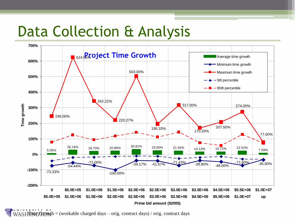
5.05%26.16% 18.73% 20.86%
30.91% 23.60% 21.55% 14.12% 15.72% 22.52%7.59%
246.00%
624.55%
342.22%
220.27%
317.00%
-35.00%-71.60%-48.00%-38.80%
-71.43%-41.67%-39.17%
-100.00%
-72.00%-54.44%
-73.33%
503.00%
274.00%
77.00%
207.50%170.33%
195.33%
-200%
-100%
0%
100%
200%
300%
400%
500%
600%
700%
0 $5.0E+05 $1.0E+06 $1.5E+06 $2.0E+06 $2.5E+06 $3.0E+06 $3.5E+06 $4.5E+06 $5.5E+06 $1.0E+07
$5.0E+05 $1.0E+06 $1.5E+06 $2.0E+06 $2.5E+06 $3.0E+06 $3.5E+06 $4.5E+06 $5.5E+06 $1.0E+07 up
Prime bid amount ($2005)
Tim
e g
row
th
Average time growth
Minimum time growth
Maximum time growth
5th percentile
95th percentile
Time Growth = (workable charged days – orig. contract days) / orig. contract days
Project Time Growth

Development of Performance Bounds
0%
10%
20%
30%
40%
50%
60%
70%
80%
90%
100%
0% 10% 20% 30% 40% 50% 60% 70% 80% 90% 100%
Time Percent Completion
Wo
rk P
erc
en
t C
om
ple
tio
n
Time/Cost Performance Curves for Successfully Completed Projects (497)
Slow Progress at 25%
Quick Start
for some
projects
Majority around
average/linear line
Cu
mu
lati
ve
Pro
gre
ss P
aym
ents
to
To
tal
Pro
ject
Val
ue
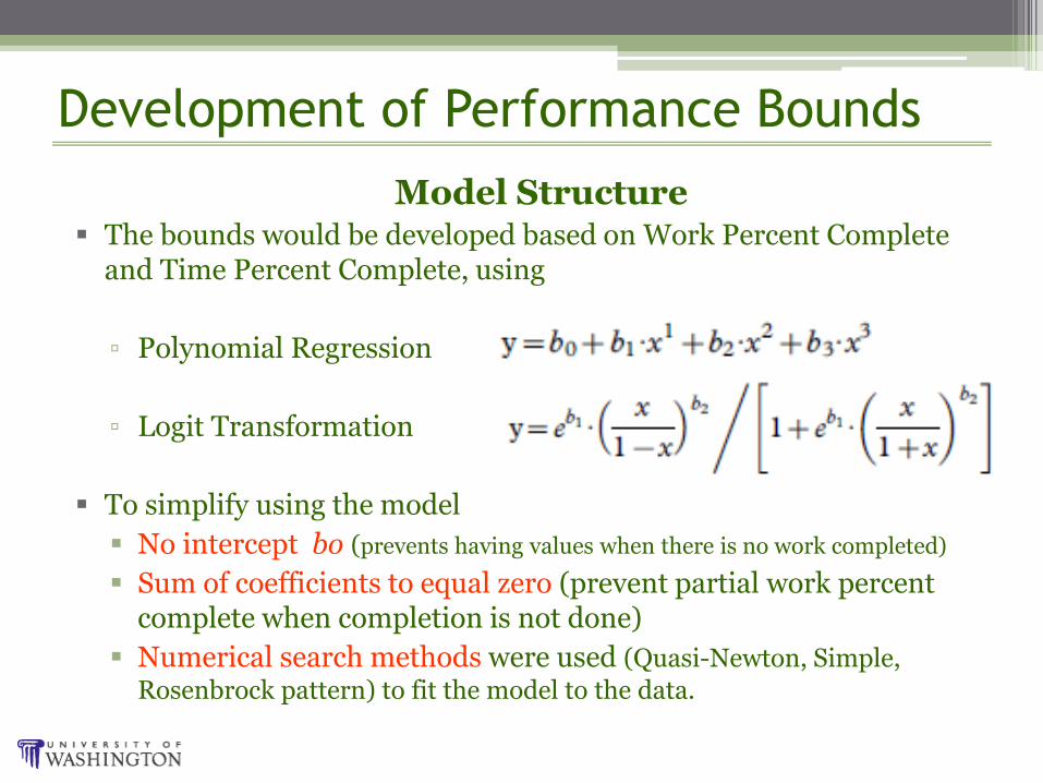
Development of Performance Bounds
Model Structure The bounds would be developed based on Work Percent Complete
and Time Percent Complete, using
▫ Polynomial Regression
▫ Logit Transformation
To simplify using the model
No intercept bo (prevents having values when there is no work completed)
Sum of coefficients to equal zero (prevent partial work percent complete when completion is not done)
Numerical search methods were used (Quasi-Newton, Simple,
Rosenbrock pattern) to fit the model to the data.

Average Performance Bounds
0% 20% 40% 60% 80% 100%
Time Percent Completion
0%
20%
40%
60%
80%
100%
Wo
rk p
erc
en
t co
mp
lete
(top down listing)y(RB3rd) =(1.19287)*x+(.006482)*x 2̂+(-.19935)*x 3̂y(Simplex3rd) =(.99762)*x+(.455684)*x 2̂+(-.45322)*x 3̂y(simplexLogit) =(exp((.236643))*(x/(1-x)) (̂1.11811)) / (1+(exp((.236643))*(x/(1-x)) (̂1.11811)))y(QN3rd)=(.943018)*x+(.52337)*x 2̂+(-.46639)*x 3̂y(linear)=x

Minimum Performance Bounds
0% 20% 40% 60% 80% 100%
Time Percent Completion
0%
20%
40%
60%
80%
100%
Wo
rk p
erc
en
t co
mp
lete
(top down listing)y(RB3rd) =(1.19287)*x+(.006482)*x 2̂+(-.19935)*x 3̂y(Simplex3rd) =(.99762)*x+(.455684)*x 2̂+(-.45322)*x 3̂y(simplexLogit) =(exp((.236643))*(x/(1-x)) (̂1.11811)) / (1+(exp((.236643))*(x/(1-x)) (̂1.11811)))y(QN3rd)=(.943018)*x+(.52337)*x 2̂+(-.46639)*x 3̂y(linear)=x
How far below the average performance would the performance is considered
unsatisfactory? No Rule. Minimum Bounds at Borders.
~20% to 30%

0% 20% 40% 60% 80% 100%
Time Percent Complete
0%
20%
40%
60%
80%
100%
Wo
rk P
erc
en
t C
om
ple
te
(top down list of profiles)
y(Rosenbrock50)=(-.01957)*x+(.258211)*x 2̂+(.761356)*x 3̂
y(Simplex50)=(-.10141)*x+(.513939)*x 2̂+(.587658)*x 3̂
y(QN50)=(-.10778)*x+(.455238)*x 2̂+(.652544)*x 3̂
(note: Rosenbrock 50 is the only +ve at the lowere tail)
Minimum Performance Bounds
Models for 50 intervals/Points

0% 20% 40% 60% 80% 100%
Time Percent Complete
0%
20%
40%
60%
80%
100%
Wo
rk P
erc
en
t C
om
ple
te
(top down list of profiles)
y(Rosenbrock100)=(.169772)*x+(.092529)*x 2̂+(.737699)*x 3̂
y(simplex100)=(-.02573)*x+(.634446)*x 2̂+(.391351)*x 3̂
y(QN100)=(.014045)*x+(.492181)*x 2̂+(.493774)*x 3̂
(note: Rosebrock and QN are +ve, Simiplex -ve at lower tail)
Models for 100 intervals/Points
0% 20% 40% 60% 80% 100%
Time Percent Complete
0%
20%
40%
60%
80%
100%
Wo
rk P
erc
en
t C
om
ple
te
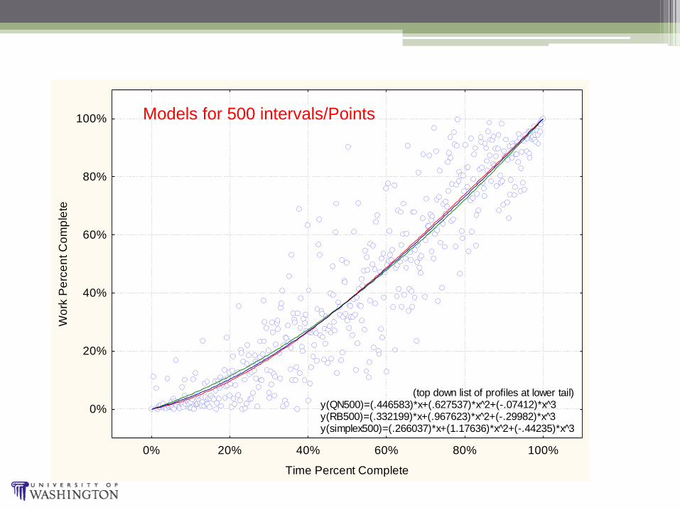
(top down list of profiles at lower tail)y(QN500)=(.446583)*x+(.627537)*x̂ 2+(-.07412)*x̂ 3y(RB500)=(.332199)*x+(.967623)*x̂ 2+(-.29982)*x̂ 3y(simplex500)=(.266037)*x+(1.17636)*x̂ 2+(-.44235)*x̂ 3
Models for 500 intervals/Points

0% 20% 40% 60% 80% 100%
Time Percent Completion
0%
20%
40%
60%
80%
100%
Wo
rk P
erc
en
t C
om
ple
tio
n
(top down list of profiles)y(Ave.Simplex.3rd)=(.99762)*x+(.455684)*x̂ 2+(-.45322)*x̂ 3y(linear)=xy(Simplex500)=(.266037)*x+(1.17636)*x̂ 2+(-.44235)*x̂ 3y(Simplex(250)=(.049248)*x+(1.16398)*x̂ 2+(-.21267)*x̂ 3y(QN100)=(.014045)*x+(.492181)*x̂ 2+(.493774)*x̂ 3y(Rosenbrock50)=(-.01957)*x+(.258211)*x̂ 2+(.761356)*x̂ 3
Models from 50 to 500 intervals/Points
Using Zero Percentiles
Zero p; extremely low
performance points

0% 20% 40% 60% 80% 100%
Time Percent Completion
0%
20%
40%
60%
80%
100%
Wo
rk P
erc
en
t C
om
ple
tio
n
(top down list of profiles)y(Ave.Simplex.3rd)=(.99762)*x+(.455684)*x 2̂+(-.45322)*x 3̂y(linear) = xy(Simplex500)=(.298511)*x+(1.22998)*x 2̂+(-.52848)*x 3̂y(Simplex250)=(.170008)*x+(1.13107)*x 2̂+(-.30072)*x 3̂y(Simplex100)=(.021358)*x+(1.0963)*x 2̂+(-.11685)*x 3̂y(Simplex50)=(-.01417)*x+(1.09372)*x 2̂+(-.07227)*x 3̂
Models from 50 to 500 intervals/Points
Using 5th Percentiles
5th p; 50 & 100 points
consistently aligned.
“True Minimum”

0% 20% 40% 60% 80% 100%
Time Percent Completion
0%
20%
40%
60%
80%
100%
Wo
rk P
erc
en
t C
om
ple
tio
n
Minimum Performance, 5th Percentile:y = (.021358)*x+(1.0963)*x^2+(-.11685)*x^3
Minimum Performance, zero Percentile:y = (.014045)*x+(.492181)*x^2+(.493774)*x^3
Linear Performance:y = x
Average Performance:y =(.99762)*x+(.455684)*x^2+(-.45322)*x^3
100-intervals Minimum Bounds
selected as benchmark to
Exclude extremely low
Performance projects
Minimum Performance Bounds

Minimum Performance Bounds
Projects are of different sizes and durations and this
would affect the shape and location of the minimum
boundary. Using Cluster Analysis, Minimum Bounds
were developed for projects classified based on:
Quantity of asphalt concrete pavement/hot mix
asphalt (ACP/HMA),
Value of contracts,
Duration of projects, and
Length (miles) of projects.

Minimum Performance BoundsContract Value
ACP/HMA Quantity
Project Duration
Project Miles

0% 20% 40% 60% 80% 100%
Time Percent Completion
0%
20%
40%
60%
80%
100%
Wo
rk P
erc
en
t C
om
ple
tio
n
(top down list of profiles)y(AvSimplex3rd)=(1.13177)*x+(.046235)*x 2̂+(-.17799)*x 3̂y(QN250)=(.30286)*x+(.615097)*x 2̂+(.082044)*x 3̂y(Simplex100)=(.144158)*x+(.475833)*x 2̂+(.380061)*x 3̂y(QN50)=(-.00136)*x+(.420091)*x 2̂+(.581271)*x 3̂
Contract Value – Small Projects
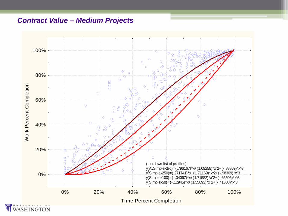
Contract Value – Medium Projects
0% 20% 40% 60% 80% 100%
Time Percent Completion
0%
20%
40%
60%
80%
100%
Wo
rk P
erc
en
t C
om
ple
tio
n
(top down list of profiles)y(AvSimplex3rd)=(.796167)*x+(1.09258)*x̂ 2+(-.88869)*x̂ 3y(Simplex250)=(.271741)*x+(1.71169)*x̂ 2+(-.98309)*x̂ 3y(Simplex100)=(-.04067)*x+(1.71582)*x̂ 2+(-.66506)*x̂ 3y(Simplex50)=(-.12945)*x+(1.55093)*x̂ 2+(-.41308)*x̂ 3

Contract Value – Large Projects
0% 20% 40% 60% 80% 100%
Time Percent Completion
0%
20%
40%
60%
80%
100%
Wo
rk P
erc
en
t C
om
ple
tio
n
(top down list of profiles)y(Ave.Simplex.3rd)=(.822014)*x+(1.35685)*x 2̂+(-1.1785)*x 3̂y(Rosenbrock50)=(.548617)*x+(1.85454)*x 2̂+(-1.4032)*x 3̂y(Simplex100)=(.477219)*x+(1.78618)*x 2̂+(-1.2626)*x 3̂y(Simplex50)=(.207607)*x+(2.29087)*x 2̂+(-1.4984)*x 3̂

Small Projects (ACP, Value, Duration, Miles)
0% 20% 40% 60% 80% 100%
Time Percent Completion
0%
20%
40%
60%
80%
100%
Wo
rk P
erc
en
t C
om
ple
tio
n
Small-projects clusters
y(ACP 100) =(.144158)*x+(.475833)*x 2̂+(.380061)*x 3̂y(ACP Av) =(1.13177)*x+(.046235)*x 2̂+(-.17799)*x 3̂y(PTC 100)=(.058828)*x+(.753789)*x 2̂+(.187899)*x 3̂y(PTC Av) =(1.00275)*x+(.390798)*x 2̂+(-.39347)*x 3̂y(WCD 100)=(.060286)*x+(.927805)*x 2̂+(.012036)*x 3̂y(WCD Av) =(1.16937)*x+(.072524)*x 2̂+(-.24188)*x 3̂y(Miles 100)=(.103791)*x+(.537874)*x 2̂+(.358704)*x 3̂y(Miles Av)=(1.03705)*x+(.251721)*x 2̂+(-.28877)*x 3̂

Medium Projects (ACP, Value, Duration, Miles)
0% 20% 40% 60% 80% 100%
Time Percent Completion
0%
20%
40%
60%
80%
100%
Wo
rk P
erc
en
t C
om
ple
tio
n
Medium-projects clusters
y(ACP 100)=(-.04067)*x+(1.71582)*x 2̂+(-.66506)*x 3̂y(ACP Av)=(.796167)*x+(1.09258)*x 2̂+(-.88869)*x 3̂y(PTC100)=(.142259)*x+(1.32259)*x 2̂+(-.46485)*x 3̂y(PTC Av)=(1.02419)*x+(.508561)*x 2̂+(-.53269)*x 3̂y(WCD 100)=(.084392)*x+(1.10427)*x 2̂+(-.17769)*x 3̂y(WCD Av)=(.79449)*x+(.976938)*x 2̂+(-.7713)*x 3̂y(Miles 100)=(-.03913)*x+(1.83751)*x 2̂+(-.79752)*x 3̂y(Miles Av)=(.669852)*x+(1.44404)*x 2̂+(-1.1139)*x 3̂

Large Projects (ACP, Value, Duration, Miles)
0% 20% 40% 60% 80% 100%
Time Percent Completion
0%
20%
40%
60%
80%
100%
Wo
rk P
erc
en
t C
om
ple
tio
n
Large-projects clusters
y(ACP50)=(.207607)*x+(2.29087)*x^2+(-1.4984)*x^3y(ACP Av)=(.822014)*x+(1.35685)*x^2+(-1.1785)*x^3y(PTC 50)=(.585584)*x+(.717461)*x^2+(-.3022)*x^3y(PTC Av)=(.871934)*x+(.774002)*x^2+(-.64587)*x^3y(WCD 50)=(.310695)*x+(1.35677)*x^2+(-.66733)*x^3y(WCD AV)=(1.0138)*x+(.473444)*x^2+(-.48687)*x^3y(Miles 50)=(.133404)*x+(2.24071)*x^2+(-1.3733)*x^3y(Miles Av)=(1.05185)*x+(.680496)*x^2+(-.73205)*x^3
ACP/HMA Quantity
Contract Value
Miles
Duration

Progress Charts
CALTRANS

Develop Conceptual Time and Cost -
Prediction Models

Time/Cost Prediction
• Assess current status/performance of prediction
• WSDOT project databases; Isolate “pavement” projects
• Assess available data and identify major variables
▫ Quantities of ACP/HMA (tons; metric and English)
▫ Quantities of Grading (tons/cy), Surfacing (tons)
▫ Length of projects (miles)
▫ Duration of projects (working days) / Contract Value
• Build prediction model using regression
▫ General Multiple Regression Models (GRM)
▫ Ridge Regression
▫ General Partial Least-squares Regression (PLS)
• Test and validate the model

Model Phase I: Preliminary Analysis
0
20,000
40,000
60,000
80,000
100,000
120,000
140,000
160,000
180,000
0 $5.0E+05 $1.0E+06 $1.5E+06 $2.0E+06 $2.5E+06 $3.0E+06 $3.5E+06 $4.5E+06 $5.5E+06 $1.0E+07
$5.0E+05 $1.0E+06 $1.5E+06 $2.0E+06 $2.5E+06 $3.0E+06 $3.5E+06 $4.5E+06 $5.5E+06 $1.0E+07 up
Paid-to-contractors dollars ($2005)
AC
P/H
MA
, to
ns
Minimum ACP/HMA
Maximum ACP/HMA
Average ACP/HMA
Variables Characteristics

Model Phase I: Preliminary Analysis
0
10
20
30
40
50
60
70
0 $5.0E+05 $1.0E+06 $1.5E+06 $2.0E+06 $2.5E+06 $3.0E+06 $3.5E+06 $4.5E+06 $5.5E+06 $1.0E+07
$5.0E+05 $1.0E+06 $1.5E+06 $2.0E+06 $2.5E+06 $3.0E+06 $3.5E+06 $4.5E+06 $5.5E+06 $1.0E+07 up
Paid-to-contractors dollars ($2005)
Pro
ject
Miles
Maximum Mileage
Average Mileage
10th percentile miles

Model Phase I: Preliminary Analysis
0
200
400
600
800
1000
1200
0 $5.0E+05 $1.0E+06 $1.5E+06 $2.0E+06 $2.5E+06 $3.0E+06 $3.5E+06 $4.5E+06 $5.5E+06 $1.0E+07
$5.0E+05 $1.0E+06 $1.5E+06 $2.0E+06 $2.5E+06 $3.0E+06 $3.5E+06 $4.5E+06 $5.5E+06 $1.0E+07 up
Paid-to-contractors dollars ($2005)
Wo
rkab
le C
harg
ed
Days (
WC
D)
Maximum WCD
Average WCD
Minimum WCD

Model Phase I: Preliminary Analysis
Best Subset Regression
Subset
#
Adj.
R2
# of
Vars
WCD Mileage ACP
ton
Grading
ton
Grading
cy
Surfacing
ton
1 0.73438 5 0.50626 0.23930 -0.31556 0.33924 0.191570
2 0.73427 6 0.50219 0.01784 0.22911 -0.32063 0.34386 0.192664
3 0.72446 4 0.54463 0.27051 -0.26336 0.42462
4 0.72424 5 0.54214 0.01153 0.26404 -0.26645 0.42791
5 0.71839 4 0.52982 0.26534 0.08018 0.141038
6 0.71815 5 0.53192 -0.01016 0.27091 0.07993 0.140878
7 0.71806 4 0.52183 0.24068 -0.06964 0.270030
8 0.71779 5 0.52323 -0.00644 0.24435 -0.06902 0.269250
9 0.71640 3 0.52819 0.25430 0.209828
10 0.71617 4 0.53058 -0.01151 0.26065 0.209399
Negative parameters
Multicolinearity is suspected

Model Phase I: Preliminary Analysis
-8 -6 -4 -2 0 2 4 6 8 10 12 14 16
Residual
-4
-3
-2
-1
0
1
2
3
4
Exp
ecte
d N
orm
al V
alu
e
.01
.05
.15
.35
.65
.85
.95
.99
Violation of the Normality
Assumption of Regression Models

Model Phase I: Preliminary Analysis
-5E6 0 5E6 1E7 1.5E7 2E7 2.5E7 3E7 3.5E7
Predicted Values
-8
-6
-4
-2
0
2
4
6
8
10
12
14
16
Sta
nd
ard
ize
d r
esid
ua
ls
Violation of the Constant Variance
Assumption
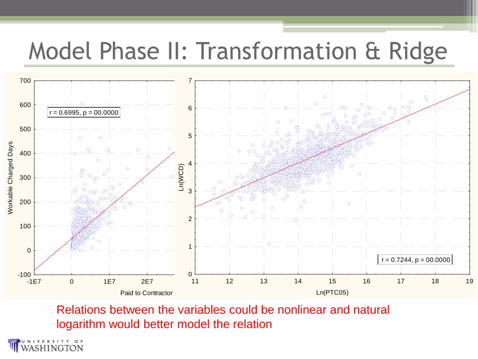
Model Phase II: Transformation & Ridge
-1E7 0 1E7 2E7 3E7 4E7 5E7 6E7
Paid to Contractor Dollars 2005
-100
0
100
200
300
400
500
600
700
Wo
rka
ble
Ch
arg
ed
Da
ys
r = 0.6995, p = 00.0000
11 12 13 14 15 16 17 18 19
Ln(PTC05)
0
1
2
3
4
5
6
7
Ln
(WC
D)
r = 0.7244, p = 00.0000
Relations between the variables could be nonlinear and natural
logarithm would better model the relation

Model Phase II: Transformation & Ridge
-1E7 0 1E7 2E7 3E7 4E7 5E7 6E7
Paid to Contractor Dollars 2005
-20000
0
20000
40000
60000
80000
1E5
1.2E5
1.4E5
1.6E5
1.8E5
AC
P T
ota
l, in
(E
), to
n
r = 0.5099, p = 00.0000
11 12 13 14 15 16 17 18 19
Ln(PTC05)
0
2
4
6
8
10
12
14
Ln
(AC
P)
r = 0.5387, p = 0.0000
Relations between the variables could be nonlinear and natural
logarithm would better model the relation

Model Phase II: Transformation & Ridge
Best Subset Regression
Subset
#
Adj.
R2
# of
Vars
Ln
(WCD)
Ln
(Mileage)
Ln
(ACP)
Ln
(Grad.tn)
Ln
(Grad.cy)
Ln
(Surf. tn)
1 0.993387 6 0.454197 -0.029436 0.417384 -0.081123 0.074937 0.154458
2 0.993347 5 0.457394 -0.030630 0.414170 -0.028739 0.177593
3 0.993340 4 0.446023 -0.030094 0.418743 0.155753
4 0.993322 5 0.444281 -0.029935 0.419584 0.005458 0.151168
5 0.993070 5 0.486856 -0.028905 0.467181 -0.074158 0.139899
6 0.993019 4 0.477137 -0.029372 0.468225 0.075002
7 0.992936 5 0.469871 0.370399 -0.088881 0.099528 0.150559
8 0.992860 3 0.467347 0.367100 0.167074
9 0.992857 4 0.504210 -0.031295 0.476289 0.040467
10 0.992855 4 0.459281 0.371939 0.023739 0.146876
Negative parameters
Multicolinearity still exist

Model Phase II: Transformation & Ridge
Ln (PTC05)
Ln (WCD)
Ln (Mileage)
Ln (ACP)
Ln (Grading
ton)
Ln (Grading
cy)
Ln (Surfacing
ton)
Ln(PTC05) 1.00 0.73 0.59 0.64 0.48 0.50 0.60
Ln(WCD) 1.00 0.30 0.38 0.53 0.51 0.53
Ln(Mileage) 1.00 0.60 0.12 0.10 0.30
Ln(ACP) 1.00 0.24 0.22 0.43
Ln(Grad. ton) 1.00 0.89 0.67
Ln(Grad. cy) 1.00 0.71
Ln(Surf. ton) 1.00
Correlation between variables
correlations between the variables were generally greater than 0.5

Model Phase II: Transformation & Ridge
Mo
del
Variables (Ln) Adj R2
MAPE Ln
(Val. Sample)
MAPE
Ln (Full sample)
MAPE
Orig.
(Full Sample)
Adj R2
Full
Sample
(1) (2) (3) (4) (5) (6) (7)
3.1 WCD, ACP, ST 0.9582 0.0546 0.08027 0.90071 0.9577
2.1 WCD, ACP 0.9433 0.0592 0.08270 0.72009 0.9425
4.1 WCD, ACP, GT, ST 0.9643 0.0629 0.07929 1.03843 0.9648
5.1 WCD, ACP, GT, GC, ST 0.9670 0.0643 0.08314 1.22998 0.9677
6.1 All including mileage 0.9669 0.0650 0.08460 1.29144 0.9677
3.2 WCD, ACP, GC 0.9557 0.0657 0.08366 0.93953 0.9562
1.2 WCD 0.8945 0.0944 0.13381 1.37117 0.8943
1.1 ACP 0.8898 0.1047 0.12341 0.64304 0.8879
Ridge Regression
No Multicolinearity; No –ve parms
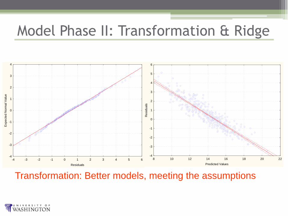
Model Phase II: Transformation & Ridge
-4 -3 -2 -1 0 1 2 3 4 5 6
Residuals
-4
-3
-2
-1
0
1
2
3
4
Exp
ecte
d N
orm
al V
alu
e
8 10 12 14 16 18 20 22
Predicted Values
-4
-3
-2
-1
0
1
2
3
4
5
6
Re
sid
ua
ls
Transformation: Better models, meeting the assumptions

Model Phase III: Relaxed Assumption
Mo
del
Adj R2 MAPE
Orig.
Inter-
cept
Ln
WCD
Ln
Mileage
Ln
ACP
Ln
Grad.
ton
Ln
Grad.
cy
Ln
Grad.
cy
6.1 0.8185 0.3446 8.9795 0.5163 0.2228 0.2178 0.0151 0.0247 0.0811
4.1 0.7736 0.3791 7.7222 0.7040 0.3255 0.0035 0.0775
5.1 0.7486 0.4060 7.8908 0.5743 0.3220 0.0040 0.0197 0.1116
5.2 0.7439 0.4187 9.2803 0.6602 0.2372 0.1094 0.0407 0.0871
4.2 0.7404 0.4201 9.5255 0.6863 0.2507 0.1190 0.0708
2.1 0.7146 0.4279 8.6080 0.8712 0.2281
2.2 0.7105 0.4391 10.1282 0.9158 0.2876
3.1 0.6909 0.4576 8.6399 0.7298 0.2091 0.0947
InterceptRidge RegressionPartial Least Squares Regression

Model Phase IV: Cluster AnalysisM
od
el Adj R2 MAPE
Orig.
Inter-
cept
Ln
WCD
Ln
Mileage
Ln
ACP
Ln
Grad.
ton
Ln
Grad.
cy
Ln
Grad.
cy
5.1 0.7696 0.2322 4.9065 0.5616 0.6662 0.0054 0.0282 0.0415
4.1 0.7844 0.2530 3.9779 0.6317 0.7457 0.0063 0.0476
6.1 0.7965 0.2550 5.8858 0.7564 -0.0092 0.5088 -0.0652 0.0697 0.0557
3.2 0.7642 0.2567 5.2735 0.8148 0.5751 0.0152
3.1 0.7670 0.2729 4.5693 0.7120 0.6563 0.0441
2.1 0.7449 0.2769 4.7516 0.7869 0.6439
4.2 0.7701 0.2955 5.3822 0.7622 -0.0009 0.5698 0.0368
5.2 0.7728 0.3000 5.4199 0.7353 -0.0203 0.5559 0.0168 0.0517 3.3 0.7625 0.3046 5.3923 0.8521 0.0086 0.5590
2.2 0.6573 0.3383 10.4916 0.9715 0.1177
K-means cluster analysis

Time Prediction
Model # Predicted WCD
MAPE
Model #
Predicted WCD
MAPE
4.3 136 18.07% P5.2 118 2.36%
5.1 135 17.25% P4.2 110 4.45%
3.1 126 9.22% P5.3 127 10.09%
4.1 129 12.49% P5.1 124 8.08%
2.2 130 13.22% P6.1 127 10.38%
3.2 114 1.01% P4.1 124 7.79%
2.3 117 1.70% P4.3 123 6.94%
3.3 129 12.26% P3.3 112 2.90%
2.1 105 8.65% P3.2 121 5.54%
3.11 112 2.25% P4.11 103 10.14%
2.4 88 23.59% P3.1 105 8.67%
4.2 148 28.80% P3.4 94 18.63%
P2.2 92 20.41%
P2.5 89 22.71%
Average 122 6.46% 112 2.62%
Std
Dev. 16
14
year Contract #
Miles PTC 05 ACP/HMA Grad. ton
Grad. cy
Surfacing Ton
WCD
1995 5159 22.26 5007423.24 45801.30 37246.43 18457.41 8281.66 115

Cost Predictionyear Contract
# WCD Miles ACP/HMA Grad.
ton Grad.
cy Surfacing
Ton PTC 05
2004 6708 110 15.92 37618.30 91823.00 91823.00 1031.30 3,382,380.43
Model # Predicted Cont Value
MAPE
6.1 $4,572,146.38 35.18%
5.2 $4,316,438.86 27.62%
3.3 $4,406,344.72 30.27%
3.2 $4,085,948.10 20.80%
4.2 $5,273,127.93 55.90%
4.1 $3,399,518.62 0.51%
2.2 $4,071,571.25 20.38%
3.1 $3,204,820.47 5.25%
5.1 $3,360,561.01 0.65%
2.1 $3,685,129.76 8.95%
Average $4,037,560.71 19.37% Std
Dev. $642,285.08