MEASURING POVERTY IN NEW ZEALAND1

Robert Stephens Senior Lecturer in Public Policy

Victoria University of Wellington

Charles Waldegrave Social Policy Consultant

Lower Hutt Family Centre

Paul Frater BERL

INTRODUCTION In Issue Four of this journal, Krishnan (1995) published a statistical analysis of trends in poverty, using six different poverty thresholds. Her analysis showed an increase in the incidence of poverty for all of the different categories of household types which can be developed from unit records of the Household Expenditure and Income Survey data base (Frater, Stephens and Waldegrave forthcoming, Stephens 1994a). However, use of the Benefit Datum Level, the 1994 married couple Invalid or Unemployed Benefit rate, or various percentages of mean and median equivalent household disposable income, by themselves, do not constitute a measure of poverty or income inadequacy due to lack of independent argument on the standard of living achieved at each poverty level. Church, welfare and community organisations have undertaken a variety of small-scale studies, documenting the living conditions of the poor, and the difficulties that these households have in making ends meet (Craig et al. 1992, NZCCSS 1995). But these studies cannot provide an estimate of the income required to avoid poverty and hardship, nor the statistical details required by policy-makers on the extent and severity of that hardship, nor information on which kinds of households are likely to be poor. Thus, it is necessary to establish an independent estimate as to what constitutes an adequate income to avoid poverty and hardship, and then relate that poverty measure to an independent statistical source. This paper sets out the New Zealand Poverty Measurement Project's method of establishing a poverty line (Frater, Stephens and Waldegrave forthcoming). Focus groups are used to establish that poverty measure, by asking households to determine an income 1 The research on which this paper is based was funded by the Foundation for Research, Science and Technology. Because of the confidentiality requirements of the Statistics Act, the statistical analysis was undertaken by officers of Statistics New Zealand, to the specification of the New Zealand Poverty Measurement Project team (the authors of this paper). Helpful comments have been received from participants in seminars at the Social Policy Agency and Victoria University of Wellington, from Jeremy Traylen and from the editors of this journal, although none, including Statistics New Zealand, are responsible for the final text.

level which will give a standard of living which provides for a minimum adequate household expenditure. A benchmark standard of living is thus developed which is both absolute in that it represents a standard of living below which households should not fall, and is relative in that it is set in relation to economic conditions within New Zealand. Changes in either economic conditions or policy parameters, e.g. charging for health services or lowering GST rates, would alter the income level required to avoid poverty. Thus the policy measure is time-specific to a given set of economic or policy parameters. The same time-specific argument indicates why the Benefit Datum Level (BDL) used by many analysts as a poverty measure (Easton 1976, 1986, 1994, Krishnan 19952, Rochford and Pudney 1984)3, 4 is no longer appropriate. Use of the BDL was initially a logical choice as the married couple benefit level was based on the Royal Commission on Social Security's (1972) expert deliberations and research on income adequacy as to the benefit level required for beneficiaries to "be able to belong to and participate in the wider community". However, economic conditions, social attitudes and public policies have significantly altered over the intervening twenty years, so that continued use of the BDL as a poverty measure no longer relates to its original conceptualisation. Even the Royal Commission (1972) argued that "poverty, need, and benefit adequacy are relative concepts", and that "the relationship between the benefit level and the selected wage level will not be fixed and immutable". Updating the 1972 benefit level by use of the Consumer Price Index (Easton 1994, Krishnan 1995) implies an absolute poverty standard, or one where the economic and social reforms from 1984 have had no impact on the required standard of living of a beneficiary. Equally, the Royal Commission relationship between benefit rates and average earnings in the 1972 formulation of benefit levels is no longer appropriate to derive a poverty measure. There have been changes in labour market conditions, especially following the Employments Contracts Act 1991; increases in female labour force participation rates resulting in a greater proportion of two-income households; plus changes in tax incidence, effective tax rates and relative prices for goods and services, especially following the tax-mix switch and tax reform of 1986 (Stephens 1993). Krishnan (1995) is correct in indicating the limitations of any poverty measure based on a percentage of mean or median equivalent disposable household income, even though they can be used for international comparisons. However, the percentage need not necessarily be arbitrary if that percentage has been derived from micro studies of household income requirements to achieve a minimum standard of living. The issue is how that percentage changes through time. Major policy changes such as tax rate changes, payment for health care and changes in low-income housing assistance would be expected to lead to different 2 Krishnan (1995) is testing the policy implications of a variety of poverty measures, and does not advocate use of the BDL. 3 Technically, officially based poverty measures should also use equivalence scales based on the degree of state support for dependants. Easton (1976), however, used New York equivalence scales adjusted for New Zealand prices, while Rochford and Pudney (1984) used the Jensen (1978) equivalence scale, and Krishnan (1995) used the Jensen (1988) equivalence scales. 4 A summary of past and recent research on both descriptive and statistical analyses of poverty is contained in Waldegrave (1994).

benchmarks set by the focus groups, giving varying percentages of median income for each year. The macro results are dependent upon the micro time-specific method of establishing the poverty line as developed in this project. This interaction between the micro poverty measure and the macro-based results represents a distinctive methodological advance in poverty measurement. Using the Unemployment Benefit as a poverty measure has some serious weaknesses. For a start, it can only indicate problems with the degree of take-up of the benefit, or that some low-income households are not covered by the social security system. Further, benefit rates are now based on the different concept of "a modest safety net" (Shipley 1991). At a practical level, there are four different benefit levels, none relating to the original formulation of the benefit level. Each benefit rate is a compromise between fiscal savings, labour force incentives and income adequacy, with the higher rate for invalids reflecting both different trade-off weights as well as differing needs through both invalidity and the expected longer duration on the benefit (Stephens 1992). This article reports on aspects of a larger study on poverty which is capable of providing consistent measurement of the incidence and severity of poverty over time, as well as identifying the efficiency of state assistance to families requiring income support (Frater et al. forthcoming). The paper commences with discussion on the use of Focus Groups to establish a consensual-based poverty measure, using a minimum adequate household expenditure notion of poverty, but related to living conditions and social attitudes of the 1990s. The next section discusses how the poverty measure was related to Statistics New Zealand's annual Household Expenditure and Income Survey (HEIS), using equivalent household disposable income. The incidence, severity and structure of poverty, before and after adjusting for housing costs for 1993, is discussed, then the household groups which are poor are identified, along with the efficiency of state assistance in reducing poverty. This is followed by an analysis of trends in both income distribution and incidence of poverty from 1984 to 1993.

ESTABLISHING A POVERTY MEASURE The poverty study interrelates a macro (or top-down) analysis of poverty using HEIS, with a micro (or bottom-up) analysis of income adequacy. In the absence of the micro component of the research, which anchors the analysis in the experience of those who live on low and/or inadequate income, any macro measure of poverty (such as percentage of median income) is arbitrary and more of a reflection of income distribution than poverty. While there is a variety of techniques to establish a micro-based poverty measure (Stephens 1988), it was felt that the poverty level should be based on actual expenditure patterns combined with subjective experiences of the population in achieving a given standard of living. Most consensual-based (or subjective) poverty measures use a direct survey, asking respondents to relate sufficiency of disposable income levels to household welfare

attainments (Hagenaars 1986). Democratic values and citizenship rights thus enter into the establishment of the poverty level (Veit-Wilson 1987). However, Walker (1987) notes that "opinions grounded in ignorance, while interesting in themselves and sometimes valuable predictors of behaviour, have little utility as a basis for policy, not least because they are likely to be unstable." He found that attitudes to the appropriate level of social security benefit levels changed in either direction when respondents were given information on the actual level of benefits. Most consensual poverty lines are very generous for the first adult, but have low equivalence scales for additional household members (Whiteford 1985). Because individuals need time to grapple with the complexities of the subject of minimum adequate income, and researchers have to provide respondents with the information they need to make reasoned choices, Walker (1987) suggested that "the consensual definition of a monetary poverty line would be derived from the deliberations of a series of group discussions. Groups, perhaps in the first instance homogeneous with respect to family type and income, would be asked to agree (through a process of negotiation) accepted minimum baskets of goods and services, and hence budgets, based on their own notion of adequacy." Walker was recommending the use of focus groups to provide an alternative method of developing a subjective poverty measure. "Focus groups are group discussions organised to explore a specific set of issues" (Kitzinger 1994): in this case, the sufficiency of a household budget to achieve a minimum adequate household expenditure. A facilitator enabled the groups to estimate a standard of living which would permit the household to "survive adequately with minimal participation":5 adequate survival implies that the family has sufficient income to purchase its own food and clothing, pay for its utilities and rent without going into debt, or needing to visit foodbanks, or take out special benefits. Meals out, videos, holidays and luxury spending are not possible. Minimum participation means that the family can take part in church, school and local activities, but not visit a restaurant or cinema. Focus groups provide a basis for different household types, cultural communities and economic status to develop an interactive view as to the income level required to achieve the defined standard of living. The participants bring their own expertise, knowledge and experience to the determination of living standards. By using existing social networks, a high level of interaction between participants is encouraged, with significant sharing and challenging of experiences and expenditure levels. Focus groups are given a choice. Some start with their own estimates of budgeted expenditures for normal purchases, and through the process of (downward) negotiation from their own expenditures, come to an agreed estimate of expenditure required to achieve the given standard of living. Others begin by defining the concept of "minimum

5 The second set of focus groups found the concept "minimum adequate household expenditure" easier to understand, and this was subsequently substituted for the original formulation, without having any impact on the results.

adequate income", and from that come up with expenditure patterns which could be compared with their actual expenditures. Both approaches gave similar results. Focus groups have been used in a wide range of social science settings, facilitating systematic comparisons of one individual's experience with those of others. They provide a more realistic social setting where the diversity of opinion, and questioning of and by participants encourages a greater sense of reflection with thought-out responses (Hedges 1985, Morgan 1988, Stewart and Shamdasani 1990). The group context provides opportunities to clarify responses, to probe questions and to ask follow-up questions (McLennan 1992). The focus group approach in this study has been used as a qualitative research method to provide a quantitative result, which measures poverty in the experience of those living on low incomes. It parallels focus group work in the UK to measure the cost of children (Middleton et al. 1994).

Focus Group Results Two sets of focus groups have so far been undertaken. (A third set, with more household types and locations, has been undertaken and results are currently being analysed. This will test whether the results based on one major urban area give any bias to the estimate). The first set was based on single-parent households in Porirua, Wellington (Cody and Robinson 1993), with a mix of interviews and focus group studies. The second set used different facilitators, different Wellington suburbs (Lower Hutt and Wainuiomata), and a wider range of household types, ethnic compositions and income levels (Waldegrave and Sawrey 1993). Table 1 shows the household characteristics of this second set, with varying proportions of one and two-parent families, income source, housing tenure arrangements, and age of oldest householder. The Porirua set were all single parent families with two or three dependent children, mainly beneficiaries in State housing, and in the younger age groups.

Table 1 Focus Groups: Sample Composition and Characteristics (%) Focus Group Type

Characteristics Māori Samoan

Pākehā Low

Income Single Parent

Low- Wage

Earner

Pākehā Middle

Income Household Size (People) 3-8 2-4 1-4 2-4 3-5 2-5 Two-Parent Families (%) 100 50 30 0 75 100 Main Income Source Wages 34 25 40 15 100 100 Benefits 66 75 60 85 0 0 Housing HCNZ 17 75 60 33 50 0 Private rental 17 25 0 17 25 0 Self-owned 66 0 40 50 25 100 Age of Householder 20-29 0 50 0 33 0 0

30-39 17 25 14 17 50 14 40-49 50 25 58 33 50 43 50-59 17 0 28 17 0 43 60+ 17 0 0 0 0 0 Source: Waldegrave and Sawrey 1993 Table 2 provides the estimate of the minimum adequate household expenditure for a household of one adult and three children from the Porirua households, along with the specification of the standard of living to be achieved. The householders stressed that these expenditure levels implied access to good information on the income and expenditure options available to the household, and that the household would have to manage its affairs extremely well if it was to survive on these expenditure levels. Disruptions such as illness or damage to assets would result in financial difficulties and the incurring of debt or reduction in other expenditures, with clothing and food most likely to be cut back.

Table 2 Estimate of Minimum Adequate Household Expenditure, Porirua, March 1993, Households of 1 Adult and 3 Children

Item Specification $/week % of Budget

Food Three meals a day for all members, plus snacks after school. Does not allow for meals for visitors. Food of supermarket quality sufficient to maintain health and normal development.

100

26 Housing Actual state housing rentals, older children of different sexes in separate bedrooms. 100 26 Power/energy Continuous hot water supply and normal use of all appliances. One room warm during

the day in winter. 20-25 6 Telephone Rental plus toll calls for those without a car and with most family outside of the

free-calling area. If not applicable, expenditure transferred to activities or transport. 10-15 3 Other household operation

Maintain cleanliness and hygiene. Utensils and cutlery for all members. Feeding and caring for pets. TV licence. 25 7

Appliances Basic set of appliances: fridge, washing machine, TV, jug, iron, toaster, radio, vacuum cleaner, drier and heaters. Maintain in operational condition and replace with new or good second-hand. 10-20 4

Furniture/ furnishings

Furnish all rooms. Beds, linen etc. for all members of the household, plus carpets, curtaining. 10-15 3

Medical Consult doctor or chemist when symptoms cause concern. Obtain medicine when prescribed. Regular medical checks at recommended intervals. Dentist not included. 5 1

Transport Public transport in the locality or contribution to cost of private transport provided by others. 15 4

Clothing and Footwear

Three summer and winter sets of clothing for each member of the household, plus additional items for recreational activities. Two pairs of shoes per year per household member. All basic items purchased new. 20-25 6

Activities and recreation.

Two members participate in one activity per week in area. 20 5

Exceptional/ emergency

Provision to avoid an unforeseen cost of less than $100 destabilising household budget, e.g. accidents, legal costs. 10 3

Education To meet fees and costs of activities common to all pupils. 8 2

Insurance Able to replace property in event of fire, theft, damage. 5 1 Life Assurance Ability to maintain a minimum standard of living and accumulate cash for future

requirements, e.g. superannuation, house purchase. 7 2 Total Basic Costs 380 100 Note: The costs are based on the prevailing prices in Porirua for a household of one adult and three children under eleven years of age. A range is given when scheduling expenditure is a major issue in how the budget is managed, and mid-point used to give the weekly total. Source: Household and Focus Group interviews, Cody and Robinson 1993. Total required expenditure was estimated to be $380 per week, in March 1993, for a single parent with three dependent children under age eleven. There was strong feeling that necessary expenditures for families with older children were substantially above those listed in Table 2. Food and housing takes over half of the budget, with most other expenses being minimal, and often an average of annual expenditure. Housing expenses are based on actual expenditures for state housing, but are prior to most of the policy change from income-related state housing rentals to market-based rents. Savings through life assurance or for house purchase are minimal and not sufficient to provide for an adequate retirement pension or deposit on a house. The second set of focus groups used the same specification for "minimum adequate household expenditure", and added a more generous standard of living – "fair with adequate participation". Two different household types were used – two adults and three children and a single adult with two children – partly to check whether the Jensen (1988) equivalence scales are realistic estimates of the additional costs of children at lower income levels. Table 3 shows the results for one focus group. Māori families, to achieve both the "minimum adequate household expenditure" and the "fair with adequate participation" standards.

Table 3 Estimates of Necessary Household Expenditures, 1993, Māori Householders (Weekly Expenditures)

Minimum Adequate Household Expenditure

Fair with Adequate Participation

2 Adults + 3 children

1 Adult + 2 Children

2 Adults + 3 Children

$ % $ % $ % Food 100 21.0 70 18.7 150 23.7 Household Operation 10 2.1 10 2.7 25 3.9 Housing 150 31.6 150 40.1 150 23.7 Power 30 6.3 20 5.3 30 4.7 Phone 11 2.4 11 3.0 11 1.6 Transport 40 8.4 30 8.0 58 9.1 Activities/Recreation 15 3.2 10 2.7 38 6.0 Insurance (car, house) 12 2.4 12 3.1 13 2.1 Life Insurance 20 4.2 15 4.0 20 3.2

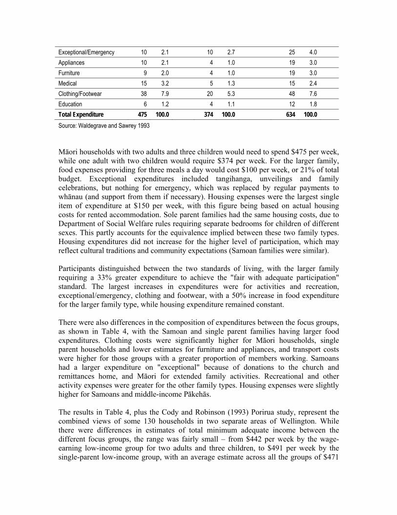
Exceptional/Emergency 10 2.1 10 2.7 25 4.0 Appliances 10 2.1 4 1.0 19 3.0 Furniture 9 2.0 4 1.0 19 3.0 Medical 15 3.2 5 1.3 15 2.4 Clothing/Footwear 38 7.9 20 5.3 48 7.6 Education 6 1.2 4 1.1 12 1.8 Total Expenditure 475 100.0 374 100.0 634 100.0 Source: Waldegrave and Sawrey 1993 Māori households with two adults and three children would need to spend $475 per week, while one adult with two children would require $374 per week. For the larger family, food expenses providing for three meals a day would cost $100 per week, or 21% of total budget. Exceptional expenditures included tangihanga, unveilings and family celebrations, but nothing for emergency, which was replaced by regular payments to whānau (and support from them if necessary). Housing expenses were the largest single item of expenditure at $150 per week, with this figure being based on actual housing costs for rented accommodation. Sole parent families had the same housing costs, due to Department of Social Welfare rules requiring separate bedrooms for children of different sexes. This partly accounts for the equivalence implied between these two family types. Housing expenditures did not increase for the higher level of participation, which may reflect cultural traditions and community expectations (Samoan families were similar). Participants distinguished between the two standards of living, with the larger family requiring a 33% greater expenditure to achieve the "fair with adequate participation" standard. The largest increases in expenditures were for activities and recreation, exceptional/emergency, clothing and footwear, with a 50% increase in food expenditure for the larger family type, while housing expenditure remained constant. There were also differences in the composition of expenditures between the focus groups, as shown in Table 4, with the Samoan and single parent families having larger food expenditures. Clothing costs were significantly higher for Māori households, single parent households and lower estimates for furniture and appliances, and transport costs were higher for those groups with a greater proportion of members working. Samoans had a larger expenditure on "exceptional" because of donations to the church and remittances home, and Māori for extended family activities. Recreational and other activity expenses were greater for the other family types. Housing expenses were slightly higher for Samoans and middle-income Pākehās. The results in Table 4, plus the Cody and Robinson (1993) Porirua study, represent the combined views of some 130 households in two separate areas of Wellington. While there were differences in estimates of total minimum adequate income between the different focus groups, the range was fairly small – from $442 per week by the wage-earning low-income group for two adults and three children, to $491 per week by the single-parent low-income group, with an average estimate across all the groups of $471

per week. Single-parent and Samoan families were noticeably younger (Table 1) so their higher expenditures may be a valid expression of the greater costs involved in establishing a household, especially with younger children. For this study, the focus methodology should establish the equivalence scales. However, insufficient family types have been used to develop equivalance scales for the wide range of family types. Moreover, the results add further weight to those who argue the imprecision of equivalence scales (Perry 1995). There is considerable variation between the focus groups as to the additional expenses of household with two adults and three children compared to a single adult with two children. To achieve the same standard of living, single-parent households estimated that the larger family required only 15% additional income compared to the smaller family, while Māori focus groups estimated the difference to be 27% and Samoans 30%, with an average of 21%. The Jensen (1988) equivalence scale, based on all incomes, implies a 38% difference in income levels between the two families to achieve the same standard of living.

Table 4 Composition of Expenditure ($) for "Minimum Adequate Household Expenditure": Two Adults and Three Children

Focus Group Type Expenditure Category Māori Samoan Pākehā Low

Income Single Parent

Low Wage Earning

Pākehā Mid Income

Average

Food 100 150 100 130 90 100 112 Household operation 10 10 10 15 10 10 11 Housing 150 180 150 150 150 180 160 Power 30 20 20 25 20 15 22 Phone 11 10 10 10 10 10 10 Transport 40 30 40 55 60 50 46 Activities 15 10 25 21 30 20 20 Insurance 11 11 15 20 15 12 14 Life Insurance 20 10 20 10 5 25 15 Exceptional 10 20 10 10 5 10 11 Appliances 10 6 4 5 10 5 7 Furniture 10 6 5 0 3 5 5 Medical 15 5 15 5 15 5 10 Clothing 37 10 15 20 20 20 20 Education 6 5 8 15 10 5 8 TOTAL $475 $483 $458 $491 $442 $472 $471 "Fair" 2A+3C 634 690 667 678 689 687 674 "Adequate" 1A+2C 374 371 377 425 390 383 386 "Fair" 1A+2C 525 563 569 547 551 Source: Waldegrave and Sawrey, 1993. It is thus debatable as to whether equivalence scales appropriate for all incomes should be used at the low end of the income distribution. The focus group estimates indicate some fixed costs of household operation, raising costs for small families relative to larger families. Use of the focus group results for two adults and three children as the basis for setting the poverty line, and adjusting it by the Jensen (1988) equivalance scale, may thus underestimate the poverty line for single adult families. There were also differences between the focus groups in terms of the different standards of living, with the wage earning low income group having the largest difference with "fair with adequate participation" being 56% greater than "minimum adequate expenditure", with the Māori group had the lowest differential at 33%. This may directly reflect community and family facilities available to Māori, and their stronger focus upon community life, rather than external, commercial activity, for entertainment. The significance of the estimate for one focus group is limited. A consistency across a number of different groups that are not in contact with each other, however, suggests a common view of budget reality on the part of those who have to live in relatively low incomes (the one middle-income group, sued for comparative purposes, came to a similar conclusion). Differences in the composition of the total budget appear to reflect different community/householder lifestyles and cultural attitudes. The results offer a sound

preliminary basis for assessing householders' opinions as to the appropriate minimum budget required for survival and for participation in New Zealand society in the 1990s. The estimates seem realistic, lying midway between a CPI update of the 1972 benefit level and 1994 Unemployment Benefit level (Krishnan, 1995). For two adults, in 1993, the focus-group-determined poverty line was almost equivalent to the Invalids Benefit level, 5% below New Zealand Superannuation, though 20% above the Unemployment Benefit level. For families with two adults and three children, receipt of the Unemployment Benefit would give them 76% of the poverty line, and receipt of the Invalids Benefit 83%, indicating that Family Support (including dependent child premium) does not fully offset the estimated additional cost of children.

SETTING THE POVERTY LINE The focus group estimate of a minimum adequate income for two adults and three children in 1993 was used as the basis for setting the poverty line. However, adjustments have been made to make the poverty line suitable for measuring poverty over time. 1) The focus groups were undertaken throughout 1993, but as inflation was low

(1.2%), the results are comparable across groups. However, rental for state housing was significantly increased in the period between the Porirua focus groups and the Lower Hutt ones. The housing rental estimates in Porirua were adjusted to reflect the implementation of the move to market rentals for state housing. The Jensen (1988) equivalence scale was also used to adjust the Porirua results to one adult and two children.

2) When the focus group results were produced, the latest HEIS data available was for the year to March 19916. This year was relatively neutral in regard to policy changes in New Zealand – the benefit cuts had been announced but not implemented7, and taxation and macroeconomic stance was consistent despite a change of government. The 1993 focus group results were deflated to 1990-91 values, using the Consumer Price Index (CPI).

3) One objective of the study was to investigate trends in poverty over the 1984-93 period of economic and social restructuring. Focus group estimates for the poverty measure obviously cannot be provided for the earlier period. The method chosen was to adjust the poverty line in relation to movements in median equivalent household disposable income, implying a relative view of poverty. Given the significant changes in policy impacting on standards of living over this period, the estimates of poverty incident are indicative only as the poverty line has been divorced from its focus group benchmark standard of living. The focus group

6 The availability of the analysis of the HEIS database will always lag behind the focus group results. In periods of rapid policy change this may give a comparability problem due to the time-specific nature of the focus group results. 7 The upward trend of numbers on the Domestic Purposes Benefit flattened out after the benefit cuts' announcement, but before their implementation.

average minimum adequate household expenditure was 59.8% of median equivalent household disposable income for 1991 (and 60.1% of median equivalent household expenditure), giving 60% as the base poverty measure8. A lower poverty estimate at 50% is also provided, giving a sensitivity analysis, and more closely related to the "modest safety net" used in setting the current benefit level.

4) Stephens et al. (1992) had argued that expenditure provided a better resource-based measure of poverty than income. However, analysis of the HEIS data base revealed that only 45.6% of households in the lowest decile by income are also in the lowest decile by expenditure, and although 22.7% are in the next decile, over 10% of the poorest by income are in the top three deciles by expenditure. When equivalence scales are used, only 26.1% of those in the lowest decile by equivalent income are also in the lowest decile by equivalent expenditure9. Much of the difficulty relates to the self-employed, or those with a temporary decline from normal income. Self-employed who declared losses, and those whose expenditure was more than three times their income, were omitted. Poverty estimates are made on both an income and expenditure basis, though the income data, when using unit records, is considered to be more reliable by Statistics New Zealand.

5) The Jensen (1988) equivalence scales, which mirror Whiteford's (1985) geometric mean, are used, with a higher child weighting for those over 11 years. The focus group results indicated that poorer households never get the chance to accumulate assets when the children were younger, and were thus faced with higher costs when children became teenagers.

6) Poverty estimates have also been made after adjusting for housing expenditures, partly to measure the impact of changes to low-income housing assistance (Stephens 1994b). Housing expenditures vary on the basis of age, tenure of dwelling and family size. Households with above average housing costs are more likely to be in poverty after housing costs than before, while low-income households with relatively low housing expenditure should have a lower incidence of after-housing costs poverty.

The approach is to exclude all housing related expenditures from each household's income, and then recalculate the poverty line. No adjustment has been made to the

8 Median equivalent household disposable income was calculated by adjusting each household's income by the Jensen (1988) equivalence scale, with two adults and one child set equal to 1.00. Two adults and one child were used as the base because this better approximated the average household size, and thus estimates of poverty gaps expressed in equivalent dollars would provide a better estimate of actual dollars required to eliminate poverty than the traditional use of two adults as the base. 9 McGregor and Borooah (1991) found a similar mismatch between income and expenditure in the UK for 1985, arguing that expenditure provides a better measure of well-being than income. The Eurostat (1990) uses expenditure as the basis for its poverty measurement, due to under-reporting of income, especially for low-income earners. Goodman and Webb (1995), in the UK, found that under 40% of those in the lowest income decile are also in the lowest decile by expenditure. They also found that the increase in inequality by income between 1979 and 1992 was greater than that by expenditure, a result similar to that of Frater et al. (forthcoming).

equivalence scale10. Housing costs were rent, mortgage payments, payments to local authorities, property and water rates, mortgage repayment insurance and insurance on buildings.

10 McClements (1978) developed commodity-specific equivalence scales in the UK, and showed that the exclusion of housing only had a significant impact on the single person's scale, lowering it from 0.65 to 0.59.

THE INCIDENCE AND SEVERITY OF POVERTY IN 1992-93 Eight inter-related measures of poverty are shown in Table 5. At the focus-group-determined poverty level – 60 per cent of median equivalent household disposable income – some 10.8% of households in New Zealand were poor, or 13.4% of the population. The difference between these two indicates that the incidence of poverty is greater among large households than small. There are still 4.3% of households, and 5.5% of people, below the modest safety net or 50-per-cent level11. However, the 60-per-cent expenditure measure gives a completely different result, with a poverty incidence of some 21.1% of households, and 20.4% of the population. Even at the 50-per-cent expenditure level, 12.9% of households and 12.3% of the population were classified as poor.

Table 5 Incidence and Severity of Poverty, 1992-93 Poverty Poverty Gap Poverty Incidence Reduction Efficiency Mean/Poverty Line Total Equivalent Poverty Measure Household People Household People % $m

50% Expenditure 12.9 12.3 24.9 502.24 50% Income 4.3 5.5 88.2 82.4 13.6 87.26 60% Expenditure 21.1 20.4 26.0 1,025.95 60% Income 10.8 13.4 73.2 68.4 15.8 308.51

After Adjusting for Housing Costs 50% Expenditure 16.6 16.0 31.6 676.14 50% Income 11.5 13.3 71.1 61.7 31.6 454.18 60% Expenditure 24.1 23.2 32.2 1,204.39 60% Income 18.5 20.5 58.1 51.3 29.7 826.45

Source: Derived from Department of Statistics (1994) Stephens (1994a) showed that while the incidence of poverty was higher for most household groups on the expenditure measure, the greatest difference was for those over 65. No elderly were poor, in 1990/91, using the 50-per-cent income measure, but 28% of elderly were poor on the correspondence expenditure measure. At the 60-per-cent level, the poverty incidence was 15.1% for income and 41.5% for expenditure. Analysis of HEIS shoed that over 60% of the elderly underspend their income, 20% have expenditure and income roughly equal, and only 20% have expenditure greater than income12. Explanations include:

11 The small differences in poverty incidence compared to Krishnan (1995) are due to different treatments of "outliers": both studies omit self-employed losses, and this study omits those with expenditure three times income. These exclusions may slightly underestimate poverty incidence. 12 Saunders (1994a) produces a similar discrepancy in poverty incidence between income and expenditure for the elderly in Australia. Borsch-Supan (1992) in Germany, and in the UK, DSS (1993), Hancock and Smeaton (1995) and Goodman and Webb (1995), have all shown that the relative position of pensioners in terms of income distribution has improved over the last decade, but not in terms of the distribution of expenditure. Banks et al. (1995) have shown that pensioners as a group tend to save from their incomes rather than dis-save, as is assumed in life-cycle models.

• poor reporting of expenditures by the elderly;

• that pensioners are a reasonably well-off group, due both to the relative generosity of New Zealand Superannuation and because the elderly have accumulated consumer durables;

• that there is greater lumpiness of pensioner expenditures; and

• that, with recent policy debates over the long-term viability of New Zealand Superannuation, health care charges and asset-testing of rest homes, the elderly are frightened to spend their income, so that the high incidence of poverty on the expenditure measure indicates their actual living conditions, even though their income provides them with the opportunity to achieve a higher standard of living.

After adjusting for housing costs, there is a substantial rise in the incidence of poverty, especially using the income measure: 18.5% of households and 20.5% of people have a combination of inadequate income and high housing expenditures. Many of those with relatively low equivalent incomes also have above average housing expenditures. Some of this represents a deliberate choice decision, with young couples taking out mortgages based on lifetime rather than current income. But most is due to households paying open-market rents to both public and private landlords, resulting in above-average absolute housing expenditures (Stephens 1994b). The data for 1992-93 pre-dates the full introduction of the targeted Accommodation Supplement as well as the final step towards market rents for HCNZ tenants. Until the 1993-94 data is analysed, the effect of the Accommodation Supplement on after-housing-costs poverty is not known. The columns "Poverty Reduction Efficiency" indicate the effectiveness of social security benefits in reducing the incidence of poverty, assuming no behavioural responses from the transfer payments13. The assumption is unlikely to be the case when the programme (e.g. pensions) have lasted for a long time, and have been taken into account when planning future income needs. In the absence of social security payments, the household incidence of poverty would have been 40.3% at the 60% income level, but fell to 10.8% after receipt of social security benefits, giving a poverty reduction efficiency ratio of 73.2%. The pre-transfer poverty incidence for people is lower at 36%, but the post-transfer poverty rate is higher, giving a lower efficiency estimate, thus indicating that large families have better access to market income, but receive less assistance from the state. At the 50-per-cent income level, social security payments are naturally more effective, reducing the household poverty incidence from 36.6% to 4.3%. After adjusting the poverty measure for housing costs, the poverty reduction efficiency estimates are substantially lower. The severity of poverty, as measured by the poverty gap in equivalent dollars, is greater using expenditure than income. At the focus group determined poverty measure, the mean poverty gap is 15.8% of the poverty line (which, for the average couple with one 13 The formula is based on after-tax income, and is calculated as (Incidence before social security benefits – Incidence after receipt of social security benefits) / Incidence before social security benefits. Mitchell (1991) uses poverty gaps, and compares pre-tax market income with disposable income, allowing calculation of the separate impacts of the tax and social security systems.

child, means that income would be about $50 per week less than the poverty line). The total poverty gap is $308 million, or just 0.43% GDP. After adjusting for housing costs, both the mean and total poverty gaps are much larger, rising to $826 million, or 8.2% of social security expenditure and 1.09% of GDP. This poverty gap estimate means that if resources could be targeted precisely to those in need, and the source of their need, then benefit levels (including family support) would be raised by $308 million, and housing assistance, through the Accommodation Supplement, a further $518 million.14 At the lower 50-per-cent income poverty level, the total poverty gap is only $87 million before housing costs, but those who are poor have an income that is on average 13.6% below that poverty line. After adjusting for housing costs there is a substantial increase, with the total poverty gap rising to $454 million, and mean poverty gap being 31.6% of the poverty line. Both mean and total poverty gaps are much larger on the expenditure measure, especially before housing costs.

Who Are the Poor? Using income as the poverty measure, Table 6 looks at the incidence and structure of poverty by household type, before any adjustment is made for housing costs. Sole parents have the highest incidence: 46.2% at the focus-group-determined poverty level. The structure of poverty indicates that they account for only 22.8% of the total population. Sole parents account for only one-fifth of the total poverty gap, with a mean poverty gap slightly less than average. Even at the 50-per-cent level, 14.3% of sole parents are poor. However, the level of the Domestic Purposes Benefit for all bar very large sole parent families lies between the 50 and 60-per-cent levels: remaining poor sole parents must be either on low wages or not receiving a benefit. Most sole parents are not in the full-time labour market – the incidence of poverty before government transfers is 94% at the lower poverty level, and 87% at the higher level. The poverty reduction efficiency is thus reasonably high at the 50-per-cent level, but a low 46.6% at the 60-per-cent level. Table 6 Incidence Of Poverty, and Structure of Poverty and Poverty Gaps by Household

Type, 1992-93 (Income as Poverty Measure, before adjusting for housing costs) 50-per-cent level 60-per-cent level

Household Type Incidence % PRE* Structure

Poverty Pov. Gap Incidence % PRE* Structure

Poverty Pov. Gap

1 adult 4.2 92.2 20.5 14.8 9.1 83.4 17.4 18.0 1 adult + children 14.3 82.5 17.8 16.6 46.2 46.5 22.8 20.0 2 adults 1.2 96.5 9.0 15.1 3.7 88.6 10.7 11.6 2 adults + 1 child 2.8 89.2 4.1 4.7 14.0 54.1 8.1 5.9 2 adults + 2 children 4.1 80.1 9.4 11.7 12.4 49.8 11.2 10.8 2 adults + 3 children 13.9 52.2 23.0 18.6 24.1 27.2 15.7 18.1 3 + adults 1.9 88.5 5.1 5.9 4.2 77.1 4.5 4.7 3 + adults + child 6.1 74.6 11.1 12.6 13.3 55.1 9.6 10.9 Total 4.3 88.2 100.0 100.0 10.8 73.2 100.0 100.0

14 Perfect targeting would not be expected due to difficulties of precisely ascertaining individual circumstances, and would not be desirable due to adverse labour supply incentive effects of the implied 100% effective marginal tax rate.

*Poverty Reduction Efficiency Source: Derived from HEIS (Department of Statistics 1993). The incidence of poverty is highest for those with children, with the incidence increasing with number of children due in part to the lack of generosity in New Zealand's assistance to low-income and large families (Stephens and Bradshaw 1995, Waldegrave and Frater 1991). This accounts for the efficiency of the social security system falling with number of children, being a very low 27% for two adults with three or more children at the 60-per-cent level. The incidence of poverty is high also because many of those with large families are Māori and Pacific Islanders with lower incomes on average (Income Distribution Group 1990). The mean poverty gap also rises with family size, being less than average for couples with one child, but well above average for couples with three or more children, so that large families account for a greater proportion of the total poverty gap than total poor population. Families without dependent children tend to have a very low incidence of poverty, though single adults make up about 20% of the total poor. There are significant difference sin the efficiency of the social security system to reduce the incidence of poverty. The poverty reduction efficiency ratio is above 80% for single and two adult households, which is largely a reflection that the old-age pension is marginally above the 60-per-cent poverty level. Mitchell (1991) argues that if countries with high poverty reduction rates also have high pre-transfer poverty rates, then there is substitution between state and market provision. The same would appear to be the case for analysis by household type. Pensions over 65 have a poverty reduction efficiency of 95.6%, reducing the incidence of poverty from 79.6% before government transfers to 3.5% afterwards, whereas those under 60, where allegiance to the work force is meant to be stronger, have a 46.6% reduction. Households where at lease one member is working have only a 52.3% reduction in poverty incidence, but the after-transfer poverty rate is only 4.2%. On the other hand, those households with nobody in the full-time work force have a 75% reduction in poverty incidence, but the after-transfers poverty rate is still 20.9%. The poverty reduction measure is not a sufficient measure of the efficiency of the social and economic system, and the post-transfer poverty rate has also to be included as an indicator of effectiveness.

TRENDS IN POVERTY THROUGH TIME

The impact of changing economic and social conditions on the incidence and severity of poverty depends on whether poverty is seen in an absolute or relative sense15. In periods of economic growth, use of a relative poverty measure will not influence poverty unless there is a change in income distribution. The incidence of poverty on an absolute measure falls with economic growth. Use of a relative standard in a recession, with falling average standards of living, implies that the living conditions of the poor should also fall. But the poor are less able to adjust their standards of living, indicating that an absolute standard may be more appropriate during recessions. However, if the decline is long term, then the poor, along with the rest of society, will have to adjust to the lower standard of living, giving a relative view. Table 7 shows that the median equivalent disposable income has fallen by 17.1%, from $32,064 in 1983/4 to $27,391 in 1992/3. The decline in standards of living is reasonably similar in the bottom five deciles by equivalent household disposable income, although the smaller fall for the second decile is due to the preponderance of superannuitants in that decile. A difficulty relates to the interpretation of the 1988 results, where many deciles have improvements in their standards of living, as these results are after the tax-mix switch, with cuts in personal income tax rates, introduction of GST and consequential price level rises. The impact of the benefit cuts in 1991/92 is seen only in the first decile, otherwise low-income groups has a consistent reduction in disposable income over the decade. There were smaller declines for the sixth to eighth decile, dominated by full-time, full-year workers, with most of that decline occurring between 1984 and 1986, while the ninth decile maintained its real disposable income and the tenth gained some 13.5%. This widening of the income distribution has resulted in an increase in the Gini coefficient of inequality from 0.255 to 0.30316.

Table 7 Trends in Income Distribution ($) – 1984 – 1993 Real 1991 Prices by Decile of Equivalent Household Disposal Income

Decile Boundary 1984 1986 1988 1990 1991 1992 1993 % Change 1 18,165 17,723 17,888 16,929 17,425 15,661 15,934 -14.0 2 20,797 20,558 20,283 19.145 18,566 187,628 18,522 -12.3 3 23,951 23,790 23,145 21,907 21,094 20,679 20,066 -19.4 4 27,793 27,096 26,766 25,184 24,611 23,517 23,328 -19.1

Median 5 32,064 30,884 31,434 29,942 29,353 27,525 27,391 -17.1 6 36,740 34,679 36,373 34,634 33,803 32,630 32,536 -12.9 7 43,339 39,186 41,398 40,294 39,876 38,417 38,800 -9.1 8 49,138 46,006 47,911 49,008 47,338 46,098 46,142 -6.5 9 59,525 56,057 56,812 60,838 59,013 57,261 59,253 -0.5

(mean) 10 71,164 68,392 70,895 84,547 84,466 77,233 83,427 13.5

15 Ideally, this issue should be resolved by the focus groups themselves. Hagenaars (1986) found that the public perception of poverty in a variety of European countries was midway between the absolute and relative views. It is postulated that in a recession, more of an absolute view will be taken, and more relative with economic growth. The next round of focus groups may shed some light on this issue. 16 Confirming evidence for this trend in inequality is found in Martin (1995), Mowbray and Dayal (1994), and Saunders (1994b), and has resulted in New Zealand having the largest reported increase in inequality amongst OECD countries (Hills 1995).

Mean 35,844 34,227 35,019 35,854 35,104 33,342 34,015 -5.4 Gini Co-efficient 0.255 0.224 0.253 0.291 0.295 0.291 0.303 -15.8

Source: Derived from Department of Statistics (1992, 1994). This fall in median income is due to the combined impact of changes in economic conditions and public policy parameters. These have affected both aggregate economic activity and the distribution of income, especially at the middle and lower ends. The focus group perception of what would have been a minimum adequate household expenditure over that period, to give a benchmark poverty level for each year, will never be known. At best, one can postulate two alternative standards – that the poverty line moves relative to median income, or that it remains fixed in absolute, real $ terms. Neither of these approaches can take account of perceptions of what constitutes an adequate income, nor the impact of the distributional effects of policy change. Thus the data in Table 8 is indicative only: it does not indicate that the New Zealand Poverty Measurement Project team advocates 60 per cent of median equivalent disposable household income as its poverty measure. This is merely a convenient expression. A fixed percentage is probably realistic during a period of little policy change, but new focus groups will be required to establish a new benchmark in periods of social and economic policy change. The forthcoming tax cuts, and recent economic growth, may result in a lowering of the focus group benchmark relative to median income. If one takes a purely relative view of poverty, then the consequence of what is a dramatic fall in the poverty level is that the incidence of poverty, before adjusting for housing costs, falls from 13.7% in 1983/4 at the higher poverty level to 10.8% in 1992/3 (Table 8). At the lower (50-per-cent income) poverty level, the overall incidence remains constant at 4.3%. With the relative poverty analysis, for most household types there is reasonable consistency in their incidence of poverty through time. For lone parents and couples with three or more children, the incidence at the 50-per-cent income level is generally above 10%, partly due to low income and partly a response to the relatively low level of assistance given for dependent children. Generally, the poverty incidence is lowest for those without dependent children. At the 60-per-cent income level, lone parents consistently have the highest poverty incidence, with a jump in 1991/2 as the benefit cuts take the Domestic Purposes Benefit substantially below the poverty level. The poverty incidence for couples with children does not show the same change, due to a greater attachment to the labour force. The introduction of Family Support in 1986 appears to have made little difference, except perhaps for couples with three or more children. There is a significant drop in the poverty incidence for single adults. Old-age pensions were maintained in nominal dollar terms, and following the 6.7% fall in the real poverty level between 1991 and 1992 due to the benefit cuts, pensions were then equal to the poverty level. This factor more than accounts for the fall in overall poverty incidence between 1990/91 and 1992/93.

Table 8 Trends in the Incidence of Poverty (%), 1984-93 (Income as Poverty Measure, Before Adjusting for Housing Costs)

50% Income Level

Household Type 1983/4 1985/6 1987/8 1989/90 1990/91 1991/2 1992/3

1 adult 3.7 3.0 2.9 2.0 2.1 3.7 4.2

1 adult + children 11.8 10.7 12 9.5 11.7 9.0 14.3

2 adults 1.7 1.0 1.2 1.6 1.7 1.8 1.2

2 adults + 1 child 4.1 2.3 1.7 1.6 3.1 5.6 2.8

2 adults + 2 children 6.6 3.1 3.6 2.8 4.1 7.3 4.1

2 adults + 3 children 14.0 10.1 6.8 5.5 12.7 10.5 13.9

3 + adults 1.3 1.2 1.8 1.6 1.1 0.5 1.9

3 + adults + children 2.7 3.5 2.1 2.6 6.5 5.2 6.1

Total 4.3 3.1 2.9 2.5 3.7 4.1 4.3

($)Real Poverty Level 50% 16,032 15,442 15,717 14,971 14,677 13,763 13,696

60% Income Level

Household Type 1983/4 1985/6 1987/8 1989/90 1990/91 1991/2 1992/3

1 adult 27.5 31.7 31.2 33.6 25.9 8.6 9.1

1 adult + children 37.8 30.3 32.8 41.8 35.8 48.6 46.2

2 adults 6.4 2.7 7.3 3.8 4.0 3.4 3.7

2 adults + 1 child 9.3 5.3 7.1 12.4 11.0 12.3 14.0

2 adults + 2 children 12.4 8.9 8.9 12.2 13.3 15.2 12.4

2 adults + 3+ children 28.1 25.6 21.2 20.1 21.8 22.0 24.1

3 + adults 2.7 2.7 2.4 2.8 3.3 1.0 4.2

3 + adults + children 5.5 9.4 6.2 6.3 12.9 8.0 13.3

Total 13.7 12.6 13.9 14.4 13.7 10.1 10.8

($)Real Poverty Level 6% 19,242 18,533 18,861 17,966 17,612 16,510 16,366 If an absolute poverty standard is taken, then a substantial increase in poverty between 1984 and 1993 is shown. In 1984, the real poverty line was $16,032 at the 50-per-cent level, and in 1993 the real poverty line at the 60-per-cent level was very similar at $16,366. Thus in absolute terms, the incidence of poverty more than doubled from 4.3% in 1984 to 10.8% in 1993. Using this absolute measure, and comparing 1984 with 1993, the incidence of poverty has increased for all household types. The most dramatic increase has been for lone parents, with a poverty incidence rising from 11.8% in 1984 (50-per-cent level) to 46.2% in 1993 (60-per-cent level). The increase has not been so dramatic for couples with children, possibly indicating a combination of greater labour force attachment plus the introduction of the targeted family support tax credit in 1986 for low-wage families.

THE ETHNIC COMPOSITION OF POVERTY The information in Table 9 supports Krishnan's (1995) analysis that Māori and Pacific Islanders have poverty rates well above the average. At the 60% poverty level, Māori poverty incidence of 27.3% is three times that of Pākehā, with Pacific Islanders being four times greater. However, Pākehā still constitute over 60% of the poor population, and a slightly larger proportion of the total poverty gap. The severity of poverty is very even between the ethnic groups, though at the 50%, Māori and Pacific Islanders have a significantly lower mean poverty gap.

Table 9 Ethnic Composition of Poverty, 1992-93 (Income as Poverty Measure)

Poverty Incidence Poverty Poverty Gap

Total

After Transfers

Before Structure

Poverty Efficiency

Reduction % P.Line

Mean ($) ($M)

Ethnic group 50% Median Equivalent Disposable Income

Pākehā 3.2 34.4 61.6 90.6 15.0 60.7

NZ Māori 10.6 54.2 21.6 80.4 11.7 16.7

Pacific Island 15.3 53.8 12.6 71.5 9.2 7.7

Other 5.8 26.5 4.2 78.1 20.4 5.7

100.0 90.8

60% Median Equivalent Disposable Income

Pākehā 8.5 37.8 63.4 77.5 15.7 205.0

NZ Māori 27.3 58.4 21.5 53.2 15.4 68.3

Pacific Island 35.8 61.5 11.4 41.8 15.0 35.1

Other 12.9 31.9 3.7 59.6 19.4 14.3

100.0 322.7

Source: Derived from Statistics New Zealand (1994) There are also substantial differences in the poverty reduction efficiency, at both poverty levels, with Pākehā having a far greater poverty reduction from social security transfers than Māori, and with Pacific Islanders having the least. The lower Pākehā poverty incidence (after transfers) is only partly a function of this greater poverty reduction efficiency. Pākehā also have a lower poverty rate before government transfers at 37.8%, compared to 58.4% for Māori and 61.5% for Pacific Islanders. This indicates the higher unemployment levels, and lower wage rates, among the latter groups. Demographics also influence the efficiency measures: Pākehā have a greater proportion of pensioners, where the poverty reduction efficiency is greatest, while Māori and Pacific Islanders have large families, where the poverty reduction efficiency is lowest.

CONCLUSIONS This paper has provided an indication of the types of analysis which the New Zealand Poverty Measurement Project team has so far undertaken. The project's distinctive methodology is to combine micro measures of households' living standards with macro statistics. Focus groups were used to develop a poverty standard which would provide households with a minimum adequate expenditure. The evidence suggests that this is a more robust method for setting a consensual poverty line than direct survey questionnaires. The result is time-specific poverty measure, dependent on current social attitudes, economic conditions and policy parameters. Retrospective use of the results must be treated with extreme caution, while future focus groups will allow continuous updating of the poverty line. The approach also provides information on the adequacy of social security benefit levels and assistance to low-income families. To measure the incidence and severity of poverty, the focus group poverty line was related to unit record data from Statistics New Zealand's Household Expenditure Survey, after omitting those reporting self-employed losses and with expenditure greater than three times income. In 1993, 10.8% of households were below the focus group determined poverty line, with sole parents and large families having the highest poverty incidence. When adjustment is made for housing costs, the incidence of poverty rises to 18.5% of households and 20.5% of the population. For non-focus-group years, some method of adjusting the poverty standard was required. If it was adjusted in line with movements in median equivalent household disposable income, implying a relative view of poverty, then the combined impact of a sluggish economy, economic restructuring and a 10% cut in social security benefit levels impacting on the critical income group resulted in a 17.6% drop in median income, but no measured increase in poverty. If an absolute poverty standard is used, the incidence of poverty before adjusting for housing costs more than doubled, from 4.3% in 1984 to 10.8% of households in 1993. The social security system was effective for reducing poverty among pensioners and households without children. These groups had both a high poverty reduction efficiency and a low poverty incidence after receipt of social security benefits. But the system was less effective for those with dependent children, with poverty incidence increasing, and degree of poverty reduction falling, with number of children.

REFERENCES Banks, J., Blundell, R. and Tanner, M. (1995) "Is there a retirement savings puzzle?" IFS

Working Paper, No. 95/2. Borsch-Supan, A. (1991) "Implications of an Aging Population: Problems and Policy

Options in the US and Germany", Economic Policy, No.12. Cody, J. and Robinson, D. (1993) "What is an Adequate Income", Unpublished Report,

January. Craig, A., Briar, C., Brosnahan, N. and O'Brien, M. (1992) Neither Freedom nor Choice,

Report of the People's Select Committee, Palmerston North. Department of Social Security (DSS) (1993) Households Below Average Incomes: a

Statistical Analysis, 1979-1990/1, London, HMSO. Department of Statistics (1992, 1994) Consumer Expenditure, 1991, 1993, Wellington,

Department of Statistics. Easton, B. (1976) "Poverty in New Zealand: Estimates and Reflections", Political

Science, Vol.28, No.2. Easton, B. (1986) Wages and the Poor, Allen and Unwin, Wellington. Easton, B. (1994) Poverty in New Zealand: 1981-1993, Economic and Social Trust on

New Zealand, Wellington. Eurostat (1990) Poverty in Europe: the Facts, European Commission. Frater, P., Stephens, R. and Waldegrave, C. (forthcoming) Micro and Macro Measures of

Poverty in New Zealand, BERL, Wellington. Goodman, A. and Webb, S. (1995) "The Distribution of UK Household Expenditure,

1979-92" IFS Commentary, No.49. Hagenaars, A. (1986) The Perception of Poverty, North-Holland, Amsterdam. Hancock, J. and Smeaton, S. (1995) "Pensioner's Expenditure: An assessment of changes

in living standards 1979-1991", Age Concern Institute of Gerontology, Kings College, London.

Hedges, A. (1985) "Group Interviewing", in R. Walker (ed.) Applied Qualitative

Research, Gower, Aldershot. Hills, J. (1995) Inquiry into Income and Wealth, Vol. 2, Joseph Rowntree Foundation.

Income Distribution Group (1990) Who Gets What? The Distribution of Income and Wealth in New Zealand, New Zealand Planning Council, Wellington.

Jensen, J. (1978) Minimum Income Levels and Income Equivalence Scales, Department

of Social Welfare, Wellington. Jensen, J. (1988) "Income Equivalences and the Estimation of Family Expenditures on

Children", mimeo, Department of Social Welfare, Wellington. Kitzinger, J. (1994) "The methodology of Focus Groups: the importance of interaction

between research and participants", Sociology of Health and Illness, Vol.16, No.1. Krishnan, V. (1995) "Modest But Adequate: An Appraisal of Changing Household

Income Circumstances in New Zealand", Social Policy Journal of New Zealand, Issue 4, July.

Martin, B. (1995) "The New Zealand Family and Economic Restructuring in the 1980's",

Population Studies Centre Discussion Papers, No. 4, University of Waikato. McClements, L. (1978) The Economics of Social Security, London, Heinemann. McGregor, P. and Borooah, V. (1991) "Is Low Spending or Low Income a Better

Indicator of Whether or Not a Household is Poor: Some Results From the 1985 Family Expenditure Survey", Journal of Social Policy, Vol.21, No.5.

McLennan, R. (1992) "The OD Focus Group: A Versatile Tool for Planned Change",

GSBGM Working Paper 5/92, Victoria University of Wellington. Middleton, S. et al. (1994) "Small Fortunes: A National Survey of Expenditures on

Children", Centre for Research in Social Policy Discussion Paper, No. 225, Loughborough University of Technology.

Mitchell, D. (1990) Income Transfers in Ten Welfare States, Academic Publishing,

Aldershot. Morgan, D. (1988) Focus Groups as Qualitative Research, Sage Publications. Mowbray, M. and Dayal, N. (1994) "The Fall and Rise (??) of Household Incomes",

Social Policy Journal of New Zealand, Issue No. 2, July. NZCCSS (New Zealand Council of Christian Social Services) (1995) A Survey of Clients

of Church Based Budgeting Agencies to Investigate the Reasons Why People Seek Budget Advice, Wellington.

Perry, B. (1995) "Between a Rock and a Hard Place: Equivalence Scales and Inter-

Household Welfare Comparisons", Social Policy Journal of New Zealand, Issue Five.

Royal Commission on Social Security (1972) Social Security in New Zealand, Government Printer, Wellington.

Saunders, P. (1994a) "Personal Memo and Calculations". Saunders, P. (1994b) "Rising on the Tasman Tide: Income Inequality in New Zealand

and Australia", Social Policy Journal of New Zealand, Issue No. 2, July. Shipley, J. (1991) Social Assistance: Welfare that Works, GP Print, Wellington. Stephens, R. (1988) "Issues in the Measurement of Poverty and Standards of Living",

Economics Discussion Paper, No. 48, Victoria University of Wellington. Stephens, R. (1992) "Budgetting with the Benefit Cuts" in J. Boston and P. Dalziel (eds.)

The Decent Society? Essays in Response to National's Economic and Social Policies, Oxford University Press, Auckland.

Stephens, R. (1993) "Radical Tax Reform in New Zealand", Fiscal Studies, Vol.14,

No. 3. Stephens, R. (1994a) "The Incidence and Severity of Poverty in New Zealand, 1990-91",

GSBGM Working Paper 12/94, Victoria University of Wellington. Stephens, R. (1994b) "The Impact of Housing Expenditures on the Incidence and

Severity of Poverty in New Zealand", GSBGM Working Paper 11/94, Victoria University of Wellington.

Stephens, R. and Bradshaw, J. (1995) "The Generosity of New Zealand's Assistance to

Families", Social Policy Journal of New Zealand, Issue 4, July. Stephens, R., Frater, P. and Ward, J. (1992) "A New Zealand Poverty Measure, BERL",

Wellington. Stewart, D. and Shamdasani, N. (1990) "Focus Groups: Theory and Practice", Applied

Social Research Methods, Vol. 20. Veit-Wilson, J. (1987) "Consensual Approaches to Poverty Lines and Social Security",

Journal of Social Policy, Vol. 16, Part 2. Waldegrave, C. (1994) "An Overview of Recent Research on Poverty in New Zealand",

paper for the Comparative Research Programme on Poverty (CROP) Scientific Symposium on The Regional State of the Art Review on Poverty Research, Paris.

Waldegrave, C. and Frater, P. (1991) "A National Government Budgets of the First Year

in Office: A Social Assessment", A Report to the Sunday Forum, The Family Centre and BERL, Wellington.

Waldegrave, C. and Sawrey, R. (1993) "Minimum Adequate Income: Focus Group

Study, Part I and Part II", Social Policy Unit, The Family Centre, Lower Hutt.

Walker, R. (1987) "Consensual Approaches to the Definition of Poverty: Toward an

Alternative Methodology", Journal of Social Policy, Vol. 16, Part 2. Whiteford, P. (1985) "A Family's Needs: Equivalence Scales, Poverty and Social

Security", Research Paper No. 27, Department of Social Security Development Division, Canberra.