Measuring Productivity Dispersion:

Lessons From Counting One-Hundred Million Ballots∗

Ethan Ilzetzki†and Saverio Simonelli‡

This Draft: August 31, 2017

Abstract

We measure output per worker in nearly 8,000 municipalities in the Italian electoral processusing ballot counting times in the 2013 general election and two referenda in 2016. We doc-ument large productivity dispersion across provinces in this very uniform and low-skill taskthat involves nearly no technology and requires limited physical capital. Using a developmentaccounting framework, this measure explains up to half of the firm-level productivity disper-sion across Italian provinces and more than half the north-south productivity gap in Italy. Weexplore potential drivers of our measure of labor efficiency and find that its association withmeasures of work ethic and trust is particularly robust.JEL Classification: O47, E24, J24, Z10

Keywords: Labor productivity, development accounting, work ethic, cultural economics.

∗We thank Sevim Kosem, Sara Moccia and Giuseppe Rossitti for outstanding research assistance and Alberto Alesina,Oriana Bandeira, Francesco Drago, Alessandra Fogli, Nicola Gennaioli, Paola Giuliano, Andrea Ichino, Ethan Kaplan,Pete Klenow, Tatiana Komarova, Hamish Low, Nicola Limodio, Tommaso Oliviero, Gerard Padro i Miquel, MarcoPagano, Torsten Persson, Annalisa Scognamiglio, Ricardo Reis, Federico Rossi, Guido Tabellini, John van Reenen, Hans-Joachim Voth, Eran Yashiv, Fabrizio Zilibotti and participants at several conferences and seminars. Research was sup-ported by grants from the EIEF, STICERD and the Centre for Macroeconomics.†London School of Economics, Centre for Macroeconomics, and CEPR‡University of Naples Federico II and CSEF.

1

1 Introduction

Measuring output per worker is an important, yet challenging, task in economics. Workers’ pro-

ductivity is the main driver of income differences across countries, and its growth is the main

proximate cause for economic growth over time (Caselli 2005). Yet measuring workers’ output is

less simple than it may seem at a first glance. While it is occasionally possible to observe work-

ers’ product directly in small scale settings, e.g. an individual production line, it is more difficult

to isolate their value added from that of other factors in large scale settings, e.g. across an entire

country. It isn’t straightforward to separate workers’ contribution from that of capital or other

productive factors. Further, productivity in firms is often measured as revenue per worker, which

may confound productivity with market power or other market imperfections (Syverson 2011)

In this paper, we measure the productivity of electoral workers who counted ballots in a general

election and two referenda in Italy. We do so not out of a particular interest in vote-counting pro-

ductivity itself, but rather because the task is particularly useful in isolating workers’ productivity

in naturally-occurring data spanning an entire country. Using data on ballot counting times from

the 2013 Italian general election and two referenda in 2016, we measure electoral volunteers’ pro-

ductivity in close to 8,000 municipalities. Combined, volunteers counted more than one-hundred

million ballots. Each polling station had a fixed number of vote counters and polling stations were

designed to minimize variation in eligible voters per station. Using observed turnout, we calculate

the number of votes counted per person-hour: a direct, output-based, measure of workers’ produc-

tivity. The task is managed at the national level and is uniform across the country, with identical

guidelines in all polling stations, allowing a direct comparison of workers’ productivity across

municipalities. The task is simple, manual, and repetitive. There is virtually no physical capital

or technology involved, and it would seem that only minimal education is required to count votes

productively. Direct pecuniary incentives are identical for all volunteers and involve a lump-sum

payment that is independent of performance or time-on-task.

There are a number of advantages to a measure of output per worker derived from this setting.

First, the vote counting task is virtually identical in all polling stations across the country. This

contrasts with workers’ tasks in firms, which vary substantially even within industries and within

a given firm. Second, the task is very labor intensive and uses essentially no other factors of

production. Hence, the setting is a laboratory that isolates workers from the capital and technology

that affects, but also confounds, their productivity in most settings. Third, the task is administered

at the national level, thus controlling for (the direct effects of) regional institutional differences.

2

Fourth, workers’ direct pecuniary incentives are identical in all polling stations and isn’t linked to

performance. (We discuss indirect pecuniary incentives in Section 4.) Any remaining productivity

differences must therefore be due to workers’ ability (human capital) or intrinsic motivation to

perform the task. Fifth, the task is performed at thousands of polling stations in all parts of the

country. Productivity has been studied in highly comparable tasks in smaller scale settings, such

as an individual production line, but not at the national level, to our knowledge. Sixth, the non-

market setting insulates our measurement from market power considerations that may hamper

the direct measurement of productivity in firms.

One may not be interested in vote counting speed per se, but we believe that vote counting

productivity provides some insights on productivity in other settings. For a number of reasons.

First, our first finding is that the dispersion in Vote Counting Rates (VCR) across Italian provinces

is slightly greater than the dispersion in output per average worker across firms in each province.

Specifically, the variance in vote counting rates is greater then that of productivity in firms and the

vote counting productivity gap between northern and southern Italy is 28%, compared to a 20%

north-south labor productivity difference in firms. That a regional productivity divide exists even

in an identical task in a setting with rudimentary technology, virtually no physical capital, and sim-

ilar pecuniary and institutional incentives, suggests large productivity differences “embedded” in

the workers themselves. Second, vote counting productivity is highly correlated with productivity

in firms at the provincial level. Beyond documenting this correlation, we conduct a development

accounting exercise, as in Caselli (2005) and Hsieh & Klenow (2010), while allowing assuming a

common factor that affects both vote counting productivity and firm level productivity. In our pre-

ferred specification, factors of production (physical and human capital) explain less than a third

of the productivity variation across Italian provinces. Once the our measure of labor-efficiency is

incorporated in the development accounting exercise, we account for nearly 80% of the variation.

We then apply this framework to study the productivity gap between northern and southern

Italy. Economists have long pondered this productivity gap, as it is remarkable that it has shown

little sign of closing, more than a century after the country’s unification. We estimate that if work-

ers in the south were as efficient as a worker in the average province in the north according to our

measure, the north-south gap in measured Total Factor Productivity (TFP) would decline by two

thirds. Further, value added per worker in firms has a bimodal distribution across provinces, pri-

marily reflecting north-south differences. However, when we equalize workers’ efficiency based

on our measure, the bimodal labor productivity distribution disappears. Quantitatively, the gap

3

between the 75th and the 25th percentile province in terms of value added per worker is 21%, but

it is only 12% once our measure of labor efficiency is equalized. This suggests that a substantial

portion of the geographical dispersion in productivity may be attributable to efficiency embedded

in workers themselves.

These exercises suggest that much of the productivity dispersion in Italy can be accounted for

by labor-specific components of productivity. This leaves open the question why it is that workers

differ so greatly in their productivity. We conclude our study with some suggestive evidence in

this regard. We show that Vote Counting Rates are correlated with cultural factors such as trust

and “work ethic”. Vote counting rates are correlated with absenteeism from the workplace, even

exploiting only within-Region variation across municipalities. They also correlate with survey

measures of self-reported trust. Exploring mechanisms, we find that the share of contested votes

(when committee members disagreed on how to assign a vote) in a municipality reduces the vote

counting rate substantially in southern Italy, but not at all in the north. Moreover, contested votes

slow down the process in low-trust provinces far more than in high-trust ones. This is consistent

with the notion that trust facilitates productivity in group tasks that involve conflict resolution.

We address a number of factors that might cause a spurious correlation between vote counting

productivity and productivity in firms. First, while the vote counting task is identical across the

country in principle, the complexity of the task might be very different in practice. To address this

concern, we use rich electoral data to control for factors that might differentiate the task across

municipalities (e.g. the number of invalid and contested ballots, how close the election was, dis-

persion of votes across parties). Second, there may be differential selection of volunteers into this

task across municipalities. To address this, we polled all municipalities in Italy and obtained data

on vote counters’ characteristics. Our results are robust to controlling for workers’ characteristics

(education, employment status, age, experience). Third, vote counters may differ in their opportu-

nity cost of time. Of greatest concern is that vote counters in more productive regions have higher

wages and therefore have an incentive to complete the vote counting task more rapidly. In this

case, VCR is merely an indirect measure of firm-level productivity, rather than a separate produc-

tivity measure. Given the specific setting, opportunity cost in its most explicit form is unlikely to

be a driver of VCR. Less than 40% of vote counters are employed (a plurality is students), so that

there is less of a direct link between the opportunity cost of time and firm-level productivity. In

addition, employers are obliged to give vote-counting volunteers paid time off on the day of, and

the day following, the election, so that poll workers received wages on those days regardless of the

4

time they devoted to vote counting. Nevertheless, we use the time-series dimension of our data

to explore the importance of the opportunity cost of time. Using province level unemployment

and wages as proxies for the opportunity cost of time, we find no within-province correlation over

time between VCR and these measures of opportunity cost. Although the improvement in labor

market conditions differed greatly across provinces between 2013 and 2016, these changes had no

bearing on vote counting productivity.

Our study relates to a literature that attempts to measure productivity in large scale settings.

Measuring productivity on a national scale is challenging, as productivity is confounded with

other factors, summarized in Syverson (2011). Firm-level data often measures revenues, but mea-

sures of physical output are less common. Revenue-based measures of productivity may confound

demand factors and market power with physical productivity. This has led researchers to com-

pare firm-level productivity in industries with very uniform products and/or where productivity

based on physical output is observable (e.g. the Syverson 2004 study of the concrete industry). We

complement this literature by studying workers’ productivity in a uniform task. Our productiv-

ity measure is highly comparable across regions as we observe physical output (number of votes

counted) and inputs (number of electoral workers) directly. We measure performance in a sim-

ple, uniform, repetitive task, in a non-market setting, where differences in technology are largely

moot and demand-side factors are irrelevant. The large productivity dispersion in this setting

and its strong geographical correlation with firm-level productivity suggests that workers’ labor

efficiency may contribute substantially to observed productivity dispersion.1

Methodologically, we follow the development accounting literature, summarized in Caselli

(2005). Conclusions from the development accounting are sensitive to assumptions, including the

parametrization of the production function. However, the general consensus is that factors of pro-

duction (physical and human capital) account for less than half the variation in output per worker

across countries. Once we incorporate our measure of labor efficiency, factors of production and

labor efficiency together account for nearly 80% of the variation in output per worker across Italian

provinces, leaving only a small role for the residual.

Our study also relates to a literature in labor economics that attempts to measure and explain

1Similar in spirit is the work of Chong et al. 2014, who send letters to non-existent addresses in every country in theworld and measure “return to sender times”: a relatively uniform task. Unlike their experimental approach, our data arenaturally occurring. And while their measure relates most directly to public sector productivity, the vote-counting taskis managed at the national level and performed by volunteers who are typically not public employees; so institutions areheld constant, for the most part. Instead, we measure vote counters’ differential performance in the same institutionalsetting.

5

labor productivity across firms or regions. A major challenge is finding relatively comparable

firms or tasks. Attempts to measure workers’ productivity harks back at least to Taylor (1911). A

modern literature in labor economics measures worker productivity in small-scale experimental

and non-experimental settings (see Bandiera et al. 2011 and Bloom & Reenen 2011 for reviews of

this literature). Productivity is typically measured in a single plant and/or geographical location.

In contrast, we construct a comparable measure of worker productivity in an essentially identical

task in every municipality of a large economy. A central question in the microeconomic literature

on labor productivity is whether workers respond primarily to monetary or non-monetary (e.g.

social) incentives (Ashraf & Bandiera 2017). It is of note in this regard that compensation isn’t tied

to hours worked or productivity in our setting. Hence productivity differences are primarily due

to differences in ability or in non-monetary incentives.

Given the that workers in our setting have similar extrinsic incentives to perform the task in

a timely manner, our findings relate to the literature on intrinsic motivation in supplying work

effort. Our research thus relates indirectly to the literature on shirking (Shapiro & Stiglitz 1984),

on-the-job leisure (Paulson 2015 and Burda et al. 2016), and absenteeism from the workplace (e.g.

Ichino & Riphahn 2005).

VCR is correlated with cultural measures of intrinsic work motivation (absenteeism) and per-

formance in group tasks (trust). As such, our paper also relates to a literature on cultural causes for

differences in income per worker (Alesina & Giuliano 2015). Much of this literature harks back to

Banfield (1958) and Putnam et al. (1993), who evoke cultural factors such as trust and civicness to

explain differences in regional development in Italy. More recently, Guiso et al. (2004, 2006, 2008a,b)

have studied these factors empirically. We believe that our measure of vote counting productiv-

ity complements existing measures of intrinsic motivation in contributing to common efforts (e.g.

blood donations) but has the advantage of being cardinal: It is measured in units of output per

worker that relates directly to other quantities of interest to economic researchers. For example,

our development accounting exercise requires a measure in productivity units and illustrates the

value of having a cardinal measure of labor efficiency.

Italy is by now a canonical setting for the study of cross-regional differences in economic de-

velopment. Although sharing common national institutions since unification in 1861, large eco-

nomic and social differences persist across Italian regions. Income per capita is nearly twice as

high in northern Italy than in the south. The north’s employment rate was 70% in 2012, com-

6

pared with 53% in the south.2 Workers in the north are 20% more productive than their southern

counterparts.3 Even infant mortality–very low in Italy by international standards–is far higher in

the south.4 There is a ongoing debate on the reasons for the Mezzogiorno problem: the sluggish

development of southern Italy. (See Eckaus 1961 and Zamagni 1997 for discussions.) We show

that a substantial portion of the differences in output per worker may be attributable to workers

themselves, rather than the lower capital stock, technology, or worse infrastructure in the south.

The remainder of the paper is organized as follows. Section 2 describes the institutional setting

of the 2013 elections and the 2016 referenda, and the vote counting process. Section 3 describes

our data, including our measure of vote counting times, and provides some summary statistics.

In section 4, we translate raw vote counting times into a measure of vote counting rates that is

comparable across Italian municipalities. Section 5 provides a theoretical framework to relate vote

counting productivity to firm-level productivity. In this section, we conduct a development ac-

counting exercise to see how far our measure of labor efficiency can go in accounting for produc-

tivity differences across Italian provinces. In section 6, we study reasons for differences in vote

counting rates. Finally, Section 7 concludes.

2 Institutional Setting: Vote Counting in Italy

Our main variable of interest is vote counting times in three separate polls. The first is the Italian

general election of 2013. The second is the oil and natural gas drilling referendum of April 2016.

The third is the constitutional referendum of December 2016. We first describe each of these polls

and then discuss the vote counting process, which was similar in all three polls.

2.1 The General Election of 2013

The nationwide general election of 2013 was held on Sunday and Monday, 24-25 of February, 2013.

Modern Italian elections take place over two days. This helps avoid congestion and delays towards

polling station closing times. In the 2013 elections, polls closed at 3pm on Monday, following a full

election day on Sunday.

The elections determined 630 members of the Chamber of Deputies (Camera dei Deputati) and

2ISTAT: Noi Italia, 20133Authors’ calculations: see Section 34ISTAT: Noi Italia, 2013. Infant mortality in Calabria and Basilicata in the south was nearly twice that of Piemonte

and Lombardia in the north. The latter compare favorably with the best-performing countries in the world; the formerare close to the bottom of the high-income country league tables.

7

the 315 elective members of the Senate (Senato della Repubblica). Elections were held under an

electoral system of proportional representation with majority bonus, regulated by law 270 of De-

cember 2005. Constituencies for the Senate correspond to the 20 Italian Regions (plus 6 Senators

representing Italians living abroad). For the Chamber of Deputies, the country is divided into 26

constituencies, corresponding to the 20 Regions, with most regions containing one constituency

and with six multi-constituency Regions. Political parties may organize in coalitions (e.g. left and

right). Representation for parties and coalitions is proportional: at the national level for the Cham-

ber of Deputies and at the Regional level for the Senate. However, the largest party or coalition

receives a bonus that increases its representation to 55% of the seats, with the remaining parties

and coalitions represented proportionally within the remaining 45%. More than 40 parties partici-

pated in the election, but all viable ones were in one of four coalitions. Turnout in the election was

75% at 35 million. The important thing to note about the electoral system is that due to propor-

tional representation, the results in any given polling station were of minimal consequence for the

election as a whole.

Voters entering a polling station received ballots for the two elections and a pencil. They were

required to mark one party on each ballot, fold the ballots, and insert them into a ballot box. Figure

A.1 in the appendix shows sample Senatorial ballots from two Regions: Piemonte in the north and

Sicily in the South. While there were slight differences due to the presence of Regional parties and

in the ordering of coalitions, the ballots were similar in their design and complexity. Ballots for the

Chamber of Deputies were even more uniform across Regions.

2.2 The Oil-Drilling Referendum of April 2016

A nationwide referendum on oil and natural gas drilling was held in Italy on Sunday, April 17,

2016, with polling stations closing at 11pm. The referendum was called by nine Regional councils

in response to a law passed by the national government that allowed existing offshore drilling

facilities to remain in operation until they are fully depleted.5 The referendum asked whether the

government should stop renewing offshore drilling licenses within 12 nautical miles of the coast.

The ballot contained two options: “Yes” and “No”.

According to Italian electoral law, a turnout of at least 50% is required if a referendum is to

alter existing laws. In this case, restrictions on offshore drilling would have been adopted only if

50% of eligible voters participated and in addition the majority of participating voters voted “Yes”.

5The nine regions were Basilicata, Calabria, Campania, Liguria, Marche, Molise, Puglia, Sardegna, and Veneto.

8

Due to the turnout requirement, Prime Minister Matteo Renzi–who was opposed to the referen-

dum–called on voters to abstain. Proponents of the proposition encouraged voters to participate

and vote “Yes”. While 85% of participants voted “Yes”, turnout (at nearly 16 million) was only

31%, so that the proposition was rejected.

Voters entering a polling station received a ballot and a pencil. They were required to mark

either “Yes” or “No”. A sample of the ballot used in all polling stations in Italy is shown in Figure

A.2 in the appendix.

2.3 The Constitutional Referendum of December 2016

A nationwide constitutional referendum was held in Italy on Sunday, December 4, 2016, with

polling stations closing at 11 pm. The referendum bundled together a number of constitutional

changes relating to the size of parliament, the division of powers between the legislative bodies

and between national and regional institutions, and additional reforms. The ballot contained two

options: “Yes” and “No”, with a “Yes” vote affirming all proposed reforms. Turnout in this refer-

endum was 65%, with 59% of votes rejecting the referendum.

Voters entering a polling station received a ballot and a pencil. They were required to mark

either “Yes” or “No”. A sample of the ballot used in all polling stations in Italy is shown in Figure

A.2 in the appendix.

2.4 The Vote Counting Process

Italy is divided into 20 administrative Regions, 110 provinces, and around 8000 municipalities

(comuni). For electoral purposes, each municipality is divided into polling stations (sezioni). Clear

rules regulate the number of registered voters per polling station, with a range of 500 to 1200 voters

per polling station.6

Each polling station in the election had a 6-member committee: A president, 4 vote counters

(scrutatori), and one secretary. In the referenda, each polling station had a 5-member committee,

with 3 rather than 4 vote counters. In addition, political parties were entitled to appoint observers,

who may report irregularities, but do not take part in counting process itself.

6Municipalities with more than 2,000 registered voters were divided into polling stations of 750 (for municipalitieswith 2,001 to 40,000 voters), 850 (for municipalities with 40,001 to 500,000 voters) or 900 (for larger municipalities)registered voters. Municipalities with 1,200 to 2,000 voters had two polling stations and smaller municipalities hadone polling station. Source: MINISTERO DELL’INTERNO 2 aprile 1998, n. 117 - “regolamento recante i criteri per laripartizione del corpo elettorale in sezioni”.

9

Participation in vote counting is voluntary. Scrutatori are selected by the municipal electoral

commission (commissione elettorale comunale) from a list of volunteers. Prior to 2005, scrutatori were

selected via lottery. In the polls studied here, municipalities differed in the degree of discretion

given to the electoral commission, with lottery remaining the norm. Scrutatori must have com-

pleted eight or more years of education and must reside in the municipality where they wish

to volunteer. The president of the committee is selected by the Regional court of appeals (corte

d’appello) from a list of volunteers and must have completed 12 or more years of education. The

secretary is appointed by the president and must have completed eight or more years of education.

Scrutatori and the secretary received financial compensation of e145 for their participation in

the election and e104 in the referenda. Presidents received e187 in the election and e130 in the

referenda. Importantly, this was a lump-sum reward for the entire processes and did not depend

on the number of hours devoted to counting votes. Thus, there was no direct pecuniary incentive

to prolong the vote counting task, nor any reward for completing it rapidly.

Employers were required by law to give scrutatori a day of paid leave to compensate for their

electoral work on the actual polling days and the day following the elections (Sunday through

Tuesday in the election of 2013, and Sunday and Monday in both referenda). In addition, scrutatori

were eligible for one more day of paid leave if vote counting extended beyond midnight. Given

that polling stations closed at 3pm in the general elections, almost all polling stations completed

the task before midnight. In both referenda, polling stations closed at 11pm, so that the majority of

polling stations completed the task after midnight. Hence, in the typical polling station in all three

polls considered, employed scrutatori were paid by their employers for the Monday and Tuesday

of the week following the election.

In the general election of 2013, polls closed at 3pm on Monday February 25th in all polling

stations. All polling stations were required to follow the following procedure. First, a number of

preliminaries related to the voter registry are conducted. Turnout is computed and the list of voters

is sent to the municipality. Second, Senate votes are counted and reported. And third, Chamber of

Deputies votes are counted and reported. We therefore have two measures for vote counting time

for the general election: the time Senate results were reported and the time Chamber of Deputies

results were reported.

In the referenda, polls closed at 11pm in all polling stations. All polling stations were to follow

the following procedure. First, preliminaries related to the voter registry are conducted. Second,

votes for the referendum are counted.

10

In each election (Senate, Chamber of Deputies, both referenda), the following procedures were

to be followed. The committee counts and records one vote at a time. If a vote is contested (e.g.

by a party observer), the president is authorized to assign the vote, but must record that the vote

was contested in the register. This procedure helps ensure that contested votes don’t delay the

procedure.7 When vote counting is complete for the given election, the president or municipal

official reports unofficial results to the municipality. This is done by phone, fax, or in a small

number of municipalities by PDA application. The municipality then communicates the unofficial

result to the Ministry of Interior. Official results are then brought physically to the municipality.

The task of vote counting is manual, routine, and uniform across the country. Figure A.3 in the

appendix shows pictures from the vote counting procedure.8 Ballots are removed from the box,

unfolded, and counted one by one. This is a task that requires minimal skill and involves nearly

no physical capital and no modern technology.

3 Data

3.1 Vote Counting

The Ministry of Interior provided data on reporting times of electoral results at the municipal

level. Municipalities reported unofficial results for each polling station and each election (Senate,

Chamber of Deputies, referenda) in real time. As noted before, the unofficial results were typically

reported via phone, so they reflect vote counting times more accurately than official results, which

require physical transportation of the hard copy of results to the ministry. For each municipality,

we have two observations for the election and one for each referendum. Each observation is a time

stamp indicating the time the unofficial result from the last polling station in the municipality was

reported. From the raw data we construct four vote counting times per municipality. Municipality

i’s Senate time is the time that Senatorial election results from the last polling station in municipality

i were reported, minus 3pm–polling station closing time. Municipality i’s total time is the time that

Chamber of Deputy election results from the last polling station in municipality i were reported,

minus 3pm.9 Municipality i’s referendum time in either referendum is the time at which referendum

7We control for the number of contested votes in Section 4 and find a positive association between counting time andthe number of contested votes, as could be expected, but this correlation isn’t statistically significant. We further use theshare of contested votes in each municipality to study the causes for vote counting rate dispersion in Section 6

8These photos were taken from websites of a number of Italian municipalities. We cannot vouch for their authenticity,but communications with actual scrutatori confirm that they are representative of the nature of the task.

9In principle, we could construct a third measure: Chamber of Deputies time, as the difference between total time andSenate time. But this measure is harder to interpret as the last polling station reporting Senate results may differ from the

11

results were reported minus 11pm.

Ideally we’d observe the counting time at the average polling station, rather than the slowest

polling station in each municipality. To understand the challenge that our measure poses, imagine

that counting times at each polling station in Italy were drawn randomly from the same distri-

bution. We’d expect the average counting time in each municipality to have the mean of this

distribution and our expected outcome would be the same in all municipalities. However, larger

municipalities obtain a larger number of draws from this distribution and there is a higher likeli-

hood that they draw an unusually large value from this distribution. Thus, even if average count-

ing times were the same in all municipalities, we’d expect to find that the slowest polling station

in larger municipalities had longer counting times than in smaller municipalities. We address this

challenge in the following section.

Figure 1 shows the distribution of (total) vote counting times in the election (left-hand panel)

and the December referendum (right-hand panel).10 The distribution for the April referendum is

reported in Figure A.4 and for the Senate elections in Figure A.5, both in the appendix. The vote

counting time for the average municipality was 5 hours and 16 minutes in the election, 1 hour and

31 minutes in the April referendum, and 1 hour and 54 minutes in the December referendum. This

means that the average municipality completed vote counting at 8:16 pm in the election, half past

midnight in the April referendum, and nearly 1 am in the December referendum. We noted earlier

that there was a potential incentive to complete the task after midnight, as this gave employed

scrutatori an additional day of unpaid leave. However, very few municipalities in the election

completed counting after midnight. In contrast, in the referenda, the majority of municipalities

completed vote counting after midnight. In all cases, we do not observe an excess mass (bunching)

of vote counting times immediately after midnight, so that the incentive to extend voting beyond

midnight does not seem to have affected vote counting rates in practice. Excluding the small

number of municipalities that did report after midnight in the election or before midnight in the

referenda does not alter our results.

In the election, dinner time may have served as a focal point for ending electoral activities.

Indeed, we do see large masses of vote counting times at 7:30-8:00 and right before 9:00pm. An

important concern is that vote counting times might be affected by regional differences in dinner

last polling station reporting Chamber of Deputies results in a given municipality. This would therefore reflect a votecounting time that did not occur at any polling station in the municipality. Our results are generally robust to using thisthird measure, with slightly weaker results as could be expected from a noisy measure.

10We trimmed the 1st and 99th percentiles of the distribution to eliminate outliers.

12

times. However, we do not see any patterns (e.g. an unusual number of southern municipali-

ties around 9pm) around these times. Moreover, results are robust when using only referendum

results, where dinner time was not a factor.

3.2 Data on Vote Counters

We surveyed Italian municipalities to learn more about vote-counters’ characteristics. Municipal-

ities are required to keep a record of the identity of electoral volunteers, but aren’t required to

report these data to the Ministry of Interior. We sent an (unofficial) email to the relevant contact

in each municipality in Italy. In the email, we explained that we were conducting research and

wished to learn more about who volunteers for electoral service. We requested an anonymized list

of volunteers’ characteristics in the 2013 election. 19% of municipalities, covering 22% of polling

stations in Italy, responded. They provided information about volunteers (Presidents, secretaries,

and scrutatori) at each poling station, their age, gender, years of education, and employment sta-

tus. In addition we asked whether the President had experience in previous elections.11 Table 1

gives summary statistics of presidents, secretaries, and scrutatori in the 2013 election. Scrutatori

and secretaries were in their mid-30s on average, and over 60% were women. Presidente were

nearly a decade older on average and nearly 60% were men. Scrutatori had 12 years of education

on average, secretaries 13, and presidents 15. The average years of schooling in the general Italian

adult population is 10.1, so that vote counters had above-average education. The vast majority

of presidents participated in the vote counting process in previous elections. While the majority

of presidents and secretaries were employed, only 39% of scrutatori were in full-time employment.

Instead, 37% of scrutatori were students and nearly 9% were unemployed. The remainder were pri-

marily stay-at-home spouses. At the time, the Italian unemployment rate was around 12%, so that

the unemployed are under-represented in our sample, while students are greatly over-represented.

Only a small fraction of scrutatori were self-employed, but the self-employed comprised nearly 20%

of all presidents.

3.3 Labor Productivity in Firms

We use the ORBIS database from Bureau van Dijk to measure labor productivity in firms. The

dataset provides balance sheet information for 3.7 million Italian firms: more than half of all firms

11Table A.1 in the appendix compares municipalities that responded to our survey to the full population. The surveyappears representative.

13

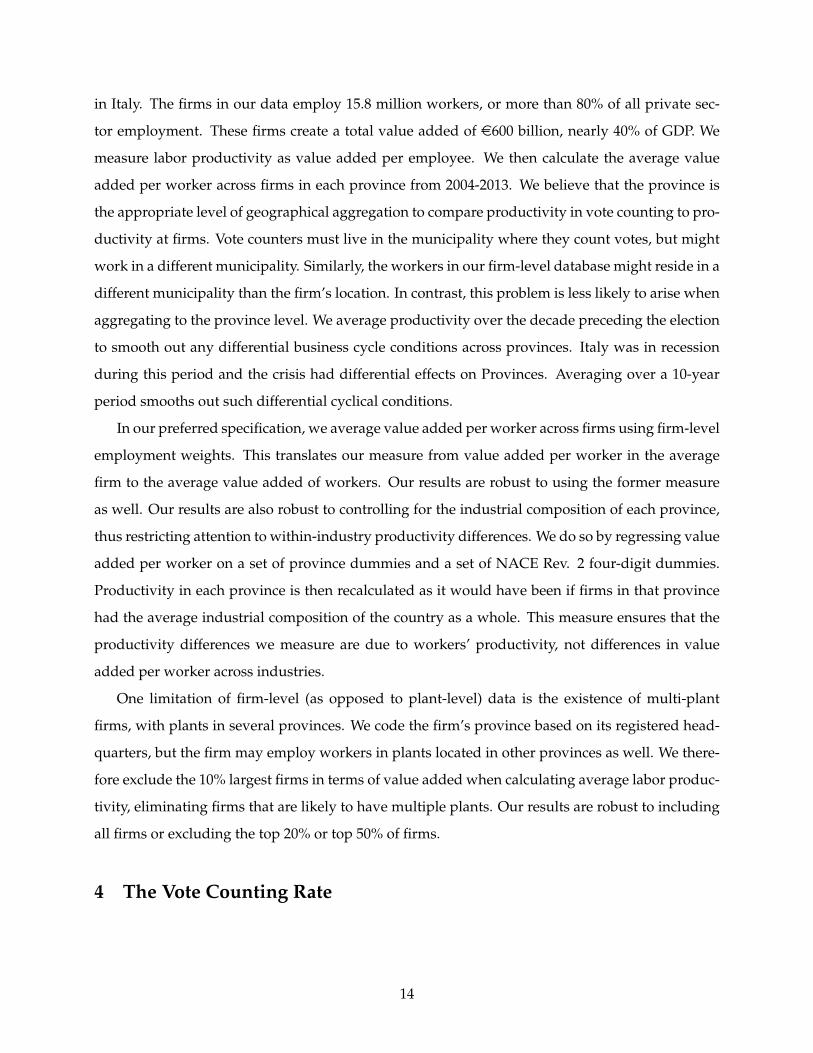
in Italy. The firms in our data employ 15.8 million workers, or more than 80% of all private sec-

tor employment. These firms create a total value added of e600 billion, nearly 40% of GDP. We

measure labor productivity as value added per employee. We then calculate the average value

added per worker across firms in each province from 2004-2013. We believe that the province is

the appropriate level of geographical aggregation to compare productivity in vote counting to pro-

ductivity at firms. Vote counters must live in the municipality where they count votes, but might

work in a different municipality. Similarly, the workers in our firm-level database might reside in a

different municipality than the firm’s location. In contrast, this problem is less likely to arise when

aggregating to the province level. We average productivity over the decade preceding the election

to smooth out any differential business cycle conditions across provinces. Italy was in recession

during this period and the crisis had differential effects on Provinces. Averaging over a 10-year

period smooths out such differential cyclical conditions.

In our preferred specification, we average value added per worker across firms using firm-level

employment weights. This translates our measure from value added per worker in the average

firm to the average value added of workers. Our results are robust to using the former measure

as well. Our results are also robust to controlling for the industrial composition of each province,

thus restricting attention to within-industry productivity differences. We do so by regressing value

added per worker on a set of province dummies and a set of NACE Rev. 2 four-digit dummies.

Productivity in each province is then recalculated as it would have been if firms in that province

had the average industrial composition of the country as a whole. This measure ensures that the

productivity differences we measure are due to workers’ productivity, not differences in value

added per worker across industries.

One limitation of firm-level (as opposed to plant-level) data is the existence of multi-plant

firms, with plants in several provinces. We code the firm’s province based on its registered head-

quarters, but the firm may employ workers in plants located in other provinces as well. We there-

fore exclude the 10% largest firms in terms of value added when calculating average labor produc-

tivity, eliminating firms that are likely to have multiple plants. Our results are robust to including

all firms or excluding the top 20% or top 50% of firms.

4 The Vote Counting Rate

14

We now translate vote counting times into a productivity measure. We define the vote counting

rate (VCR) for election s in municipality i as

VCRi,s ≡τi,svi,s

σihi,s, (1)

where hi,s is counting time for election s in municipality i in hours; τi,s is turnout as a share of

total eligible voters at the municipal level; vi,s is the number of eligible voters in municipality i

in election s; and σi is the number of polling stations in municipality s. Hence, τi,svi,s/σi is the

number of votes to be counted per polling station in municipality i and election s. VCRi,s is then

an approximation of the number of votes counted per polling station.12

A challenge with this measure is that we only observe the average number of ballots per polling

station in a municipality. This measurement problem interacts with the fact that we observe the

counting time hi,s for the last polling station in each municipality. Hence in equation (1) we are

dividing the average number of votes per polling station in municipality i with the largest vote

counting time in the municipality. We address this “last polling station” problem below.

Figure 2 shows VCR in the election on the left-hand panel and in the December referendum

on the right. (Similar figures for the April referendum and the Senate elections can be found in

Figures A.4 and A.5 the appendix.) The vote counting rate is largely in the 100-300 range and

averages 190 in the election, with a standard deviation of 65.13 Differences in vote counting rates

across polls are far smaller than differences in vote counting times. This means that the majority

of variation in vote counting times was due to differential turnout, rather than differential vote

counting productivity.

Correlation Between VCR and Firm-Level Productivity The stage is now set for an initial

comparison between vote counting productivity with productivity in the workplace. The left panel

of Figure 3 shows a map of Italy with average VCR at the province level for the elections. Shades

reflect quartiles of the VCR distribution, with darker shades reflecting faster vote counting. This

is compared with the right-hand panel, which shows the average value added per worker in each

province, again shaded by quartiles, with darker shades reflecting more productive provinces.

Vote counting was faster in the north of Italy than in the south, mirroring the north-south divide

12The number of workers is constant across polling stations, so that votes counted per worker is the same as thisfigure up to a constant.

13134 in the Senate, 145 in the April referendum, and 254 in the December referendum, with standard deviations of55, 63, and 100, respectively.

15

in labor productivity. But there is also significant within-area variation and within-area correlation

between the two variables. For example, Emilia Romagna was among the fastest in vote counting

and is among the most productive regions in northern Italy. The correlation between VCR and

firm level productivity is statistically significant. Figure A.6 shows the same information in a

scatter plot of value added per worker against VCR.

Adjusting for Task Complexity While the vote counting task is very uniform across the coun-

try, there are some factors that may make the task more challenging in some municipalities than

in others. For example, the ballot may be more complex in some Regions and some municipalities

may have a larger number of invalid votes, which require greater scrutiny by vote counters. To ad-

dress this concern, we adjust the vote counting rate for information from the electoral rolls. Table

2 shows results from a regression of (log) VCR in the election, (total time in the left panel and Senate

time on the right), on a number of factors that might affect the complexity of the task. (A similar

table for the two referenda is shown in Table A.2 in the appendix.)

We first explore whether the share of challenged votes in a municipality affected the vote count-

ing rate. As noted earlier, the polling station president is required to list every ballot that was con-

tested and proceed without delay. Nevertheless, a contested ballot may lead to a discussion among

the committee and may stall the vote counting process. As expected, municipalities with a higher

share of contested votes had slower raw vote counting rates, but the relationship is statistically

insignificant in most specifications.

Large numbers of invalid and blank ballots also appear to slow down the vote counting pro-

cess. A one-percentage point increase in the share of blank or invalid votes lowers the vote count-

ing rate by 7% in the election and more than 10% in the referenda. The committee may dwell on

such ballots, wishing to ensure that they are truly invalid or blank before proceeding.

Columns 2 and 5 include additional controls for differences in the complexity of the task. Bal-

lots with a larger number of parties may be harder to count. Hence we control for the number of

parties in the lower house and the Senate. As expected, a larger number of parties did slow down

vote counting, with an additional party causing vote counting rates to decline by 1%.

Counting votes may be easier where there is less dispersion in party affiliation. Where votes

are cast for numerous parties, including large shares for smaller parties, each ballot may require

more attention. Accordingly, we control for the dispersion of votes across parties in each of the

elections (Senate and Chamber of Deputies) using a Herfindahl index. In practice, vote dispersion

16

in votes didn’t have a statistically significant effect on vote counting rates.14

Given proportional representation, the winners at the municipal level and even the Regional

level are irrelevant for outcomes of the Chamber of Deputies. Referenda are determined at the

national level as well. While senatorial elections are Regional, they are also based on propor-

tional representation with more than one seat representing each Region,15 making the result at any

given polling station or municipality insignificant to the overall result. However, psychological

factors may induce counters to scrutinize ballots more carefully where the stakes are perceived to

be higher. We measure a close race by the difference between the vote shares of the two coalitions

with the largest vote shares, in percentage points. However, the closeness of the election doesn’t

seem to have had an impact on vote counting rates.16

For completeness, columns 3 and 6 repeat the exercise for the sample of small municipalities

with one or two polling stations. Results are essentially unchanged.

Having controlled for the complexity of the task, we use residuals from these regressions as

“Adjusted VCR”, reflecting a measure of vote counting productivity that is adjusted for the com-

plexity of the task. Figure A.7 shows the distribution of Adjusted VCR in the election (left-hand

panel) and the December referendum (right-hand panel). Similar figures for the April referendum

and using Senate time can be found in Figures A.4 and A.5 in the appendix. VCR is adjusted us-

ing the more parsimonious specification from the first column of Table 2, but the distributions are

similar when including the full set of controls.

The left-hand panel of Figure A.8 in the appendix shows that Adjusted VCR is very highly

correlated with the original unadjusted measure, with a Spearman correlation of 0.98, so that the

ranking of provinces is virtually the same by both measures. Further, Figure A.9 in the appendix

shows that value added per worker at firms remains highly correlated with VCR after adjusting

for the complexity of the task. All results that follow are also unchanged whether using the raw or

adjusted measure, so we continue to use the unadjusted raw measure in our main specification.

14The number of parties and vote dispersion are irrelevant for the referenda and therefore excluded from the regres-sion in Table A.2 in the appendix.

15An exception is Val d’Aosta with one seat and a majority electoral system.16Given the binary options in the referenda, the share of votes in favor of the proposition is perfectly correlated

(positively or negatively) with the tightness of the referendum. We include the share of “YES” votes in each referendumas a control in Table A.2. The share of “YES” votes is statistically significant in the December referendum, but ofincorrect sign, and this may be a spurious “over-control”. Prime Minister Renzi happened to be particularly popular inhigh-productivity provinces. The referendum received the highest approval rates in South Tyrol, Tuscany, and EmiliaRomagna, and these happen to be among the most productive regions in the country.

17

Last vs. Average Polling Station As we have noted, we observe the vote counting time of the

last rather than the average polling station in each municipality. This is of concern, because larger

municipalities are statistically more likely to have an outlying polling station with an unusually

large and unrepresentative vote counting time. We address this matter in two ways. First, figure

A.10 in the appendix shows estimates from a non-parametric regression of log VCR (using the

raw unadjusted measure) for each municipality on bins of the number of polling stations in each

municipality. The regression is for the election using total time, but nearly identical results arise for

the Senate and the referenda. There is some minor variation in VCR depending on the number of

polling stations, but there is no clear relationship between the number of polling stations and VCR.

Hence, there is no indication of an extreme value problem for municipalities with many polling

stations. When we control for bins of the number of polling stations, the correlation between value

added per worker in firms and VCR remains intact and all result that are reported below continue

to hold.

Second, we restrict the sample to municipalities that had at most two polling stations, elimi-

nating or diminishing the difference between last and average polling station. Unfortunately, we

lose nearly half of all municipalities in this restricted sample and eight provinces with no such

municipalities. Again, all results are robust to using this measure.

Given that the “last polling station problem” doesn’t appear to affect any reported results qual-

itatively, we proceed with the raw VCR measure, but report robustness of our main results to the

number of polling stations in the following section.

Controlling for Volunteer Characteristics (Selection on Observables) Vote counting is vol-

untary and volunteers’ characteristics may differ across the country. Of particular concern is that

volunteers in low-productivity provinces are negatively selected, creating a spurious correlation

between vote counting rates and firm-level productivity, due to selection bias. To address this con-

cern, we explore whether volunteers’ characteristics are correlated with VCR and control our VCR

measure for observables.

We surveyed all municipalities in Italy to obtain data on vote counters’ characteristics in the

2013 election. We didn’t make an official request for the data, so that response was voluntary. The

response rate was nevertheless high at 20%. Summary statistics on vote counter characteristics can

be found in Table 1. Table 3 then shows results of a regression of (log) VCR on these characteristics.

18

As before, the two panels correspond to total time (on the left) and Senate time (on the right).17

Results in the table are at the municipal level for the the nearly 1,000 municipalities that responded

and provided complete information on vote-counters’ characteristics.

We pooled the characteristics of all committee members (presidents, secretaries and scruta-

tori), but results were similar when we controlled separately for each category of polling station

worker. Vote counters’ age and gender had no substantial impact on vote counting productivity.

In contrast, measures of human capital did appear to have an important effect on vote counters’

performance. An additional year of schooling for all vote counters in the municipality increased

the pace of vote counting by 7%. Employment status also had an effect: a municipality with polling

stations comprised entirely of employed vote counters was 27% more productive than a committee

entirely comprised of volunteers who were not employed. Students were even more productive

than employed vote counters.18 Finally, experience matters. A municipality with a president with

no previous experience counted votes 10% slower than one with a president with experience from

previous elections. Finally, the regression includes controls for the vote counting process that were

used to measure the adjusted vote counting rate described earlier.19

We label residuals from this regression as “Controlled” VCR, to reflect that it controls for vote

counters’ characteristics. Figure A.11 in the appendix shows a histogram of Controlled VCR. The

right-hand panel of Figure A.8 in the appendix shows that this measure is correlated with Adjusted

VCR, with a Spearman correlation of 0.6. The correlation coefficient is highly statically significant,

but the correlation is imperfect. Provinces’ vote counting productivity ranking is slightly altered

when controlling for vote counter characteristics. Nevertheless, Controlled VCR remains corre-

lated with value added per worker at firms, as shown in Figure A.9 in the appendix. In addition,

we will show that our main results are robust to the use of this measure of VCR.

We caveat that this measure may involve over-controlling: the general population in high-

productivity provinces is more educated and more likely to be employed than in low-productivity

provinces. Hence, we might be inadvertently controlling for factors affecting labor productivity

when controlling for vote counter characteristics, rather than merely correcting for selection on

17We don’t have information about vote counters’ characteristics in the referenda so cannot conduct this exercise forthe two referenda of 2016.

18This is initial suggestive evidence that the opportunity cost of time was not important in determining vote countingrates. Presumably workers have a higher opportunity cost of time than do students, yet students counted votes morerapidly.

19Column 2 (5 for the Senate) also includes the entire set of controls that appeared in Table 2 and column 3 (6 for theSenate) includes additional dummies of bins of the number of municipalities. Results are roughly the same in all threespecifications.

19

observables.

Opportunity Cost of Time The correlation between VCR and labor productivity in firms is

not meant to represent a causal relationship. Rather, these are two separate measures of output per

worker in two different settings. One causal concern nevertheless arises, relating to the opportu-

nity cost of time. High opportunity cost of time may affect electoral workers’ incentive to finish the

vote counting task rapidly. Insofar as workers in high-productivity provinces earn higher wages,

we might expect them to have a higher opportunity cost of time and count votes faster because they

are more productive in the workplace. If this is the case, our correlations don’t reflect two separate

measures of labor productivity.

We remind the reader that there are no direct pecuniary incentives to rapid completion of the

vote-counting task. Payment is lump-sum and isn’t tied to vote counting pace. Recall also that

electoral volunteers’ employers are required to compensate them during their absence, so oppor-

tunity cost is not reflected directly in forgone wages: employed vote counters’ market income

was unaffected by the amount of time devoted to vote counting. Nevertheless, if workers choose

working hours and leisure optimally in the workplace, workers in high-wage municipalities may

nevertheless face a higher opportunity cost due to a high value placed on scarce leisure. If VCR

is higher because electoral workers with higher market wages have an incentive to complete the

electoral task faster, then our measure is simply a consequence of market labor productivity, rather

than an independent measure of productivity in a different setting.

To address this concern, we exploit the time series dimension of our data. We observe VCR in

the 2013 election of and the referenda of 2016. If VCR captures intrinsic productivity, it is unlikely

to have changed dramatically within 3 years. If, on the other hand, VCR merely captures the

opportunity cost of time then it should change with underlying economic conditions. There was

much regional variation in pace of recovery from the recession (with a business cycle trough in

2012). If the opportunity cost of time is an important factor in incentivizing rapid vote counting,

municipalities with stronger recoveries would have seen greater increases in VCR.

We measure the improvement in business cycle conditions using the change in unemployment

or alternatively the change in wages from 2013-15. Unfortunately, at the time of writing, unem-

ployment and wage data were still unavailable for 2016. The correlation between the log change

in unemployment and the log change in VCR is shown in a scatter plot in Figure 4. The figure also

presents a similar figure comparing the change in wages and VCR. The figure shows the change

20

in VCR from the election to the referendum of December 2016, but results are similar when using

the April referendum or the average VCR of both referenda.

There was much variability in the economic recovery from 2013 to 2015. In fact, provinces

were as almost as likely to experience an increase in unemployment as they were to experience

a decrease. Changes in unemployment varied widely from a decrease of more than 5 to an in-

crease of nearly 10 percentage points. There were also changes in vote counting rates, but these

largely reflect an upward shift that occurred to a similar extent in all provinces. The Spearman

correlation between provinces’ VCR in the election and the December referendum was 0.94, alone

suggesting that VCR is largely capturing a characteristic of the province, not of particular economic

circumstances. It is therefore not surprising that regressing the change in VCR on the change in

unemployment (or wages) gives a tightly estimated zero with an R-square of essentially zero. By

this test, find no evidence that the opportunity cost of time was a factor in determining VCR. Our

results are robust to using any of our VCR measures (adjusted, including population controls, or

including municipalities with less than three polling stations). It is also robust to including area

fixed effects.20

Another aspect of opportunity cost of time that might contaminate our measure is differences

in dinner time.21 Given that vote counting in the election began at 3pm and the several hours

required to count votes, dinner time could have served as an incentive, or a coordinating device,

to finish the at a specific time. We are reassured by the fact that all results in the paper are virtually

identical when using data from the referendum alone. Vote counting in the referendum began at

11pm, so that dinner time would not affect the opportunity cost of time.

5 Vote Counting Rate as Labor Productivity

There is much dispersion in firms’ productivity, even within narrow industries. This is true for the

US and even more so among emerging markets (Hsieh & Klenow 2009). Syverson (2011) reports a

65% difference between the 90th and 10th percentile plant even within narrow industries in the US.

We find similar dispersion of productivity across provinces in Italy, with a 50% difference between

the 90th and 10th percentile provinces. There have been many suggestions as to the causes of

this dispersion, including differences in production technology, the quality of labor or capital, and

20We include fixed effects for South-Center, North-East, and North-West.21Dinner times may themselves be endogenous to labor productivity, but explaining dining habits is beyond the scope

of this paper.

21

market structure.

Figure 5 shows the distribution of value added per worker across Italian provinces (in red).

This distribution is based on the average worker in each province, regardless of industry. Further,

it is a revenue-based measure of labor productivity rather than a quantity based one, with the

associated confounding factors (Syverson 2011).

The figure also presents the dispersion in VCR (in black). The dispersion is no smaller, in fact

slightly larger, than that of value added per worker. In contrast to value added per worker in

firms, VCR is a quantity-based measure of productivity, from a non-market setting, in a uniform

task that is directly comparable across the country. Given the nature of the task, differences in

VCR cannot be due to physical capital, technology, or market power. The vote counting process

is managed at the national level, so this measure also controls somewhat for (the direct effects of)

regional institutional differences. It is therefore interesting that a similar degree of productivity

variation exists in a task of this nature. Even when individuals are put in a uniform “industry”,

given a uniform task, given uniform compensation, and are sheltered from market forces, there are

large spatial productivity differences. Further, we have shown a correlation between productivity

differences in the polling station and in the workplace. This suggests a role for a productivity

factor that affects performance both in the workplace and in the simple vote counting task.

We investigate this possibility further by treating VCR and value added per worker as two

separate labor productivity measures and see how far a common factor might explain productivity

dispersion across firms in Italy. The framework we propose is a development accounting type

variance composition.22 Beyond standard assumptions in development accounting, we make three

additional assumptions that allow us to translate VCR into labor productivity in firms.

Assumption 1: Vote counters and workers within province i share a common labor efficiency

factor ei.

Assumption 2: The vote counting technology exhibits constant returns to scale in the number

of worker-hours.

Assumption 3: Labor efficiency is an exogenous worker characteristic.

The first assumption is extreme, as the vote counting task is very different from the diverse set

of tasks facing workers in firms. However, this assumption puts a larger burden on vote counting

efficiency in accounting for labor efficiency in firms, as vote counting productivity is likely a noisy

22Our methodology follows Klenow & Rodriguez-Clare (1997) most closely. See Caselli (2005) and Hsieh & Klenow(2010) for reviews of the development accounting literature.

22

measure of productivity in the workplace. Vote counting may exhibit increasing (learning on the

job) or decreasing (fatigue) returns to scale. Absent further guidance on returns to scale, we as-

sume constant returns as our second assumption. Finally, the third assumption is for expositional

simplicity.

We posit the following vote-counting production function

ni,s = eihi,sls, (2)

where ni,s is the number of votes counted in municipality i in poll (election/referendum) s; hi,s

is the number of hours devoted to vote counting; ls is the number of electoral workers per polling

station in poll s, and ei is the labor efficiency of workers in province i. The form of the production

function follows directly from the three assumptions. With this production function, equation (1)

implies that VCR is a direct measure of labor efficiency ei.

Next, we posit a production function for firms in province i. We use a standard Cobb-Douglas

production function:

Yi = AiKαi (HieiLi)

1−α ,

where Yi is the physical output of firms in province i, Ki is physical capital, Li is the number of

workers, Hi is human capital per worker, α is the labor share, Ai is total factor productivity, and

ei is labor efficiency. In framing the production function in this manner, we are assuming that ei is

a productivity measure that goes beyond traditional measures of human capital (schooling). We

have demonstrated that education does affect VCR in Section 4 and Table 3. However, with Hi

absorbing variation in traditional measures of human capital, variance captured by ei will be due

to aspects of human productivity that go beyond these traditional measures. Moreover, our results

are robust to using Controlled VCR as a measure of labor efficiency. Recall that measure controls

for vote counters’ years of schooling. Writing the production function in per capita terms gives

yi = Aikαi (Hiei)

1−α , (3)

where yi and ki are output per worker and capital per worker, respectively.

Development accounting is a decomposition of the variance in output per worker into the

variance associated with observable factors of production, while assigning the residual variation

to unobserved TFP Ai. Conclusions are sensitive to the underlying production function (Caselli

23

2005). When using a simple production function as in (3), the general consensus in existing studies

is that at least 50% of the variation in output per worker across countries remains residual variation

in TFP.

In our baseline variance decomposition, we follow Klenow & Rodriguez-Clare (1997), who use

the following measure.

Accounted Variation (Xi) =cov ( f (Xi) , yi)

var(yi),

where Xi is a vector of quantities of measured production inputs, yi is output per worker, and

f (.) is the posited production function. In words, the variation in output per worker explained

by factors of production is given by the correlation between output per worker and its predicted

value, based on the production function and observed inputs. The residual variation is given by

one minus this measure.23

In order to conduct the variance decomposition, we require measures of capital per worker and

of human capital. We measure capital per worker using the firm-level data discussed in Section 3.

Human capital is typically measured as the predicted value added of a year of schooling using a

Mincerian regression of the average years of schooling on wages using micro data.24 In his compi-

lation of international micro-level evidence on the returns to schooling, Caselli (2017) determines

that the returns to a year of schooling in Italy has been 4.6% in recent years. These are meagre

returns by international standards, so as robustness we repeat the exercise allowing for 9.5% and

15% returns, which are the average and on the higher end of the international range, respectively.

Formally, if φ is the return to a year of schooling and χi is the average number of years of

schooling in province i, then human capital is given by

Hi = eφ

1−α χi .

Finally, we use average (log) VCR in the three polls as our measure of labor efficiency ei.

Results of the variance decomposition are summarized in Table 4. The three rows correspond

to three values of returns to schooling mentioned above. A production function including capital

23Caselli (2005) proposes an alternative measure: Accounted Variation (Xi) =var( f (Xi))

var(yi). Our results are robust to the

use of this alternate measure.24Hanushek & Woessmann (2012) argue that quality of education needs to be taken into account alongside years of

schooling. As a robustness check, we controlled for average PISA scores at the province level. The quality-adjustedschooling measure of human capital increases the contribution of human capital in explaining the variance of outputper worker across provinces by around 10 percentage points, but doesn’t affect the contribution of labor efficiency ei.

24

per worker alone, yi = Aikαi , explains 22% of the of the variance in output per worker, with the

remaining 78% attributed to TFP. When human capital is included as well, yi = Aikαi H1−α

i , factors

of production now explain 25% to 35% of the variance, depending on the assumed returns to

schooling. In all cases, the majority of variation remains unexplained. However, when we add our

measure of labor efficiency to the production function, we now explain 78% of the variance in the

central scenario. With our measure of labor productivity, we can now explain well over half of the

variation in labor productivity across firms. In fact, labor efficiency alone explains nearly half the

variance.

In summary, a standard development accounting exercise suggests that a common productivity

factor present in both the vote counting task and at the firm level may be important in capturing

the variation in output per worker across Italian provinces.

Counterfactual Exercises using VCR as Labor Efficiency This framework allows us to con-

duct a number of counterfactual “experiments”, to which we now turn. The provincial distribution

of output per worker as measured in firms is shown in Figure 6. As noted in the introduction, the

distribution is bimodal, very much reflecting the north-south productivity gap. The figure also

plots the distribution in terms of efficiency units of labor, given by Yiei Li

. This distribution is “better

behaved”: The bimodal nature of the distribution is eliminated. To put the compression of the

labor productivity distribution in quantitative perspective, the 75%-25% interquartile gap (IQR) in

output per worker is 21%, but it is only 12% in value added per efficiency units of labor. Thus, our

measure cuts the interquartile difference by nearly half.

Thinking along north-south lines, we conduct the following counterfactual exercise. Value

added per worker is 20% higher in northern Italy than in the South, measured from firm data. We

wish to assess how far our measure of labor efficiency can go in accounting for this productivity

gap. To answer this question we conduct the following counterfactual exercise. We assign the

median labor efficiency of northern provinces to all southern provinces whose labor efficiency is

below the northern median. Under this counterfactual, using our theoretical framework, the north-

south gap in output per worker would decline to 7%, cutting the north-south labor productivity

gap by more than half.

Robustness We conducted a series of robustness checks, summarized in Table 5. For each

specification we report the results of our main three exercises. First, we calculate the IQR in value

25

added per efficiency unit according to the associated measure. Second, we calculate the north-

south difference in labor productivity, corrected for labor efficiency as described above. Third, we

report the residual from the development accounting exercise, i.e. the remaining unexplained vari-

ation after capital, human capital, and labor efficiency are incorporated in the production function.

For sake of comparison, the first row reports results uncorrected for labor efficiency. As noted,

the IQR of the distribution of value added per worker is 21% and the north-south labor produc-

tivity difference is 20%. In addition, recall that 69% of the variance of output per worker remains

unexplained in a developing accounting exercise that includes physical and human capital (using

the middle scenario for returns to schooling). The second row repeats the results reported above

from our baseline specification. In our preferred specification, accounting for labor efficiency cuts

the IQR by half, the north-south productivity gap by nearly two thirds, and the development ac-

counting residual by two thirds.

The remaining rows report results from robustness tests. Our main specification averages VCR

from the three polls (total election time, April referendum and December referendum). We repeat

the analysis for each poll separately. Results are strengthened substantially when restricting at-

tention to the election or the December referendum. In particular, the development accounting

exercise now explains nearly 100% of the variation in output per worker across provinces. Con-

versely, the April referendum gives slightly weaker results, but the message remains the same.25

We next report exercises that test robustness to the “last polling station problem”. Results are

robust to using a VCR measure that controls non-parameterically for the number of polling stations

and a measure that includes only municipalities with less than three polling stations. (See Section

4.) Finally, results are robust to VCR measures adjusted for the complexity of the task and that

control for vote-counter characteristics.

Assuming a common productivity factor that appears in both the vote counting task and in

firms, we find that this factor accounts for much of the cross sectional variation in output per

worker in Italian firms. What factors might drive this underlying productivity. We turn to possible

determinants of vote counting productivity next.

25Results using the Senate election only perform even better than using total time in the election.

26

6 What Drives Vote Counting Rates?

As a measure of labor efficiency, VCR shows large dispersion and geographical variation that is

correlated with productivity in firms. With the simple theoretical framework we outlined in the

previous section, labor efficiency was able to account for a significant share of the variation in out-

put per worker. Development accounting exercises search for proximate causes for the variation

in output per worker across countries or regions. In their seminal development accounting study,

Hall & Jones (1999) go further in exploring correlates with the TFP residual in an investigation of

root causes for productivity differentials across countries. They argue that productivity differences

are driven by what they label “social infrastructure”. In their words, social infrastructure is

The institutions and government policies that determine the economic environment

within which individuals accumulate skills, and firms accumulate capital and produce

output. A social infrastructure favorable to high levels of output per worker provides

an environment that supports productive activities and encourages capital accumula-

tion, skill acquisition, invention, and technology transfer. Such a social infrastructure

gets the prices right.

We don’t dispute the importance of social infrastructure, but the large dispersion in vote-

counting productivity we have found refines what might explain productivity differentials in our

setting. Incentives and “prices” in the vote counting task itself are equally right (or wrong) across

the country in that volunteers were given no incentive to count votes rapidly. Whatever drove

vote counters’ ability or motivation to complete this task efficiently must have carried over from

broader institutional and cultural factors driving labor efficiency.

What, then, drives labor efficiency in such a simple task as counting votes? We begin by reca-

pitulating a number of hypotheses that we believe we can be rejected outright in this setting. We

then explore some more plausible explanations. First, production technology and physical capi-

tal (private or public) are unlikely explanations for differences in VCR. The vote counting process

requires a table, chairs, writing implements, and a building. While there might be minor regional

variation in the quality of these work tools, it is hard to see how they would make an enormous

impact on vote counting speed. Essentially no technology is involved. Literate workers from the

pre-industrial era would have been able to complete this task with the technologies available to

them at the time. Caselli (2017) suggests that some of the international difference in output per

27

worker may be due to differences in production technology (e.g. capital or human capital inten-

sity). However, in our setting, the production technology is essentially the same across the country.

Turning to incentives, the direct pecuniary incentive–financial compensation–is identical in all

polling stations. Further, compensation is lump-sum and not linked to the amount of time spent

counting votes. Vote counters may differ in the opportunity cost of their time. However, we

showed in Section 4 that VCR wasn’t correlated with measures of the opportunity cost of time.

More plausible explanations for regional differences relate to those that are worker-specific

and would affect productivity in the workplace but also translate to other settings. These include

cultural attitudes towards work, broader measures of culture that might affect work performance

in group settings, and human capital. The nature of the task and the fact that we are using naturally

occurring data makes it difficult to disentangle these factors. We nevertheless try to shed some light

with suggestive correlations shown in Table 6. This table shows results from a panel regression of

(log) VCR (pooling the election and both referenda) on a number of variables may capture these

underlying factors. All regressions include fixed effects for each of the referenda. Area fixed effects

are also included, so that the regressions are based on within Area variation across municipalities

rather than a comparison between say North and South Italy.

We first consider attitudes towards work, by looking at absenteeism from the workplace. We

measure absenteeism using municipal level data on the number of sick leave days taken by public

employees. We follow Ichino & Riphahn (2005) and others who have considered variations in sick

leave as measuring shirking in the workplace. Table 6 reports a statistically significant and negative

relationship between VCR and absenteeism. This regression is robust to including fixed effects for

the 22 Italian Regions (not reported here). Municipalities with more workplace absenteeism also

counted votes more slowly. This correlation provides some possible insights on the forces affecting

both absenteeism and VCR. High rates of absenteeism are often seen as driven by high value

placed on off-the-job leisure. For example, people have a greater incentive to be absent from work

in cultures that place a higher value on time with family. The correlation between absenteeism with

VCR casts absenteeism in a different light. Absenteeism is greater where votes are counted more

slowly, thus where vote counters forewent more off-the-job leisure while engaged in the electoral

task. This correlation is thus inconsistent with absenteeism and VCR driven solely by valuing off-

the-job leisure. An alternative hypothesis fits more neatly with this correlation. Absenteeism and

low efficiency in vote counting may reflect a high cost to exerting work effort or lower psychic costs

to shirking: low “work ethic”. Variation in work ethic would lead to a correlation between demand

28

for off-the-job-leisure on one hand and shirking on the other. In this perspective, absenteeism is

driven more by an aversion to being at work than by the attraction of being at home.

We next turn to broader cultural factors. A large literature studies the role of culture in af-

fecting attitudes, economic policy, and economic outcomes. In the Italian context, Banfield (1958)

suggested lack of trust outside of the family circle–termed amoral familialism–as an impediment

to the economic development of the Italian south. Putnam et al. (1993) studies the historical role of

lack of trust or civicness. More recently, Guiso et al. (2004) have shown that trust is an important

factor in financial development and the development of trade relations and have studied the role

of civic-mindedness on economic performance in Guiso et al. (2008a).26 Turning first to civic duty,

we use a commonly used measure of civic mindedness: blood donations.27 One might expect a

positive correlation between blood donations and VCR. The same cultural attitudes that drive cit-

izens to donate blood might encourage them to devote a greater effort in a voluntary group task,

particularly one that is related to the democratic process. As expected, blood donations are posi-

tively correlated with VCR. However, the association becomes weak and statistically insignificant

when including additional controls.

Next, we measure “trust” using survey data collected for the World Value Survey.28 VCR is

correlated with trust with a statistically significant coefficient. A theoretical literature suggests

that trust might affect performance in group tasks, particularly where workers’ efforts are strate-

gic complements.29 The vote counting task features strong strategic complementarities. All vote

counters are required to scrutinize each ballot and agree on assigning the vote. We will explore

one mechanism, through which trust affects vote counting empirically below.

These regressions are robust using Adjusted VCR or Controlled VCR as the productivity mea-

sure. The latter controls for human capital as measured by employment status and education.

However, human capital may affect vote counting productivity through a different channel, that

of organizational capacity. We found some suggestive evidence that managerial capacity mattered

in Table 3, as experienced presidents presided over faster vote counting. To explore this channel

26Aghion et al. (2010) have suggested that lack of trust could lead to over-regulation (which in turn makes it harderfor trust to develop). See also discussion in Tabellini (2008, 2010) on the interaction between trust and institutions.

27Number of blood bags per million inhabitants. The indicator ranges from 0 to 0.11. Source: Guiso et al. (2004). Wethank Luigi Guiso for sharing his data.

28The survey was conducted across 2,000 Italian households in the 1990s. Respondents were asked how much theytrusted other Italians in general. Responses were on a scale of 1 to 5, with 5 indicating that they trust them completelyand 1 indicating that they do not trust them at all. The measure is then normalized to range from zero to one. We thankLuigi Guiso for sharing these data.

29However, much of the existing literature focuses on “vertical trust” between workers and supervisors or employers.See Wintrobe & Breton (1986) for a discussion.

29

further, we use the management score from Bloom & Van Reenen (2007, 2010), but see an essen-

tially zero correlation between VCR and management quality in firms.3031

In summary, we find some suggestive evidence of the role of work ethic through a negative

correlation between VCR and absenteeism. We also find a correlation between VCR and survey

measures of trust. We now take a closer look at the role of trust in affecting VCR.

Trust and Labor Productivity in a Contentious Task We further investigate the mechanism

through which trust affects VCR by looking closer at the vote counting process. As we saw in Table

2, the share of contested, blank, or invalid votes in a municipality slowed down the vote counting

process. These factors likely affect VCR because they add to the complexity of the task and require

judgement calls. However, we assumed that the complexity of the task had similar effects across

the country. We now investigate whether these factors had heterogeneous effects in the north and

the south of Italy, in Table 7. This is pooled regression of (log) VCR on the these three factors in

the election and the two referenda, interacted with broad area dummies (north and south-center).

Challenged votes slowed down the vote counting rate in the south and center of Italy, but not in the

north. The effect is statistically significant and large in the south: an increase in challenged votes

by one percentage point slows down vote counting by nearly 25%. At the median southern VCR,

this implies a reduction from counting 157 votes to only 120 votes per hour. In contrast, blank and

invalid votes slow vote counting down by similar margins in both northern and southern Italy.

Why would contested votes have such a substantial effect on vote counting rates in the south

but not in the north? We conjecture that trust plays a role in explaining this difference. Officially,

the procedure for dealing with contested votes requires the President to assign the vote provi-

sionally and indicate that the vote was contested in the register. In high trust environments, the

committee may agree with this provisional assignment quickly. In low trust environments, each

contested vote may lead to a debate on how to assign the provisional vote. We explore this possi-

bility by interacting the number of contested votes with the survey measure of trust, in the third

column of Table 7. Challenged votes slow down the vote counting process, and VCR is higher in

high-trust provinces, as previously established. Specifically, the gap between the most- and least-

trusting provinces is 0.3, so that trust may increase vote counting rates by up to 50%. However,

when interacting the share of challenged votes with the measure of trust, we find that trust is

30The management score is only available at the Regional level. With merely 20 observations on this variable, theregression may lack statistical power.

31For completeness, we show that results are robust when controlling for latitude, in an attempt to further control forfactors that differ across north-south lines.

30

particularly important where there are more challenged votes. Specifically, a one percent increase

in challenged votes decreases vote counting rates by 35% in municipalities in the least trusting

province, but this declines to merely 6% in the most trusting provinces.32. The contested task of

adjudicating contested votes slows down the vote counting process substantially where trust is

low, but only slightly where trust is high.

These findings provide suggestive evidence of the role of trust in labor productivity, directly

from the vote counting task. Vote counting is a group task and the law requires consensus in

assigning a vote to a particular party. Contested votes reflect a potentially conflictual component

of the task and they may impede consensus. We find that trust, measured by a general social

survey, may aide the group in reaching consensus.

7 Conclusions

We measure output per worker in the vote counting process of the Italian election of 2013 and two

referenda in 2016. The vote counting task is simple, uniform, and easily comparable across mu-

nicipalities. The task involved no physical capital or modern technology and minimal skills. The

process was governed at the national level and provided workers with identical incentives. We

argue that this measure captures labor-specific efficiency that is clean from many of the confound-

ing factors when measuring output per worker using firm level data. We nevertheless find that

this measure shows similar geographical dispersion as does labor productivity in firms and the

two measures are correlated. We conduct a simple development accounting exercise and find that

our labor efficiency measure accounts for nearly half of the variation in output per worker across

provinces. Equalizing labor efficiency would substantially compress the provincial dispersion in

labor productivity and would halve the north-south productivity divide. Vote counting productiv-

ity is correlated with separate measures work ethic and trust. Exploring mechanisms, we find that

trust is important in increasing productivity with aspects of the task that may be more conflictual.

We hope our measure will be of use to future empirical researchers. Our measure captures

efficiency in a group task, is available for all Italian municipalities with three observations in two

separate years. The task is measured in units of output per worker. Our development account-

ing exercise illustrates the utility of having a cardinal measure of what is potentially a cultural

attribute. This exercise should be replicable in other countries where the vote counting process

32“Trust” ranges from 0.62 to 0.92

31

is similarly uniform across the country and we hope that future research will find use for the

methodology proposed here in other settings.

32

References

AGHION, PHILIPPE, ALGAN, YANN, CAHUC, PIERRE, & SHLEIFER, ANDREI. 2010. Regulation

and Distrust. The Quarterly Journal of Economics, 125(3), 1015–1049.

ALESINA, ALBERTO, & GIULIANO, PAOLA. 2015. Culture and Institutions. Journal of Economic

Literature, 53(4), 898–944.

ASHRAF, NAVA, & BANDIERA, ORIANA. 2017. Social Incentives in Organizations. Mimeo. London

School of Economics.

BANDIERA, ORIANA, BARANKAY, IWAN, & RASUL, IMRAN. 2011. Field Experiments with Firms.

The Journal of Economic Perspectives, 25(3), 63–82.

BANFIELD, EDWARD C. 1958. The Moral Basis of a Backward Society. Glencoe, IL: The Free Press.

BLOOM, NICHOLAS, & REENEN, JOHN VAN. 2011. Chapter 19 - Human Resource Management

and Productivity. Handbook of Labor Economics, vol. 4, Part B. Elsevier.

BLOOM, NICHOLAS, & VAN REENEN, JOHN. 2007. Measuring and Explaining Management Prac-

tices Across Firms and Countries. The Quarterly Journal of Economics, 122(4), 1351–1408.

BLOOM, NICHOLAS, & VAN REENEN, JOHN. 2010. Why Do Management Practices Differ across

Firms and Countries? Journal of Economic Perspectives, 24(1), 203–24.

BURDA, MICHAEL, GENADEK, KATIE R., & HAMERMESH, DANIEL S. 2016 (January). Not Working

at Work: Loafing, Unemployment and Labor Productivity. Working Paper 21923. National Bureau of

Economic Research.

CASELLI, FRANCESCO. 2005. Accounting for Cross-Country Income Differences. Chap. 9, pages

679–741 of: AGHION, PHILIPPE, & DURLAUF, STEVEN (eds), Handbook of Economic Growth. Hand-

book of Economic Growth, vol. 1. Elsevier.

CASELLI, FRANCESCO. 2017. Technology Differences over Space and Time. Princeton University Press.

CHONG, ALBERTO, PORTA, RAFAEL LA, DE SILANES, FLORENCIO LOPEZ, & SHLEIFER, ANDREI.

2014. Letter Grading Government Efficiency. Journal of the European Economic Association, 12(2),

277–299.

33

ECKAUS, RICHARD S. 1961. The North-South Differential In Italian Economic Development. Jour-

nal of Economic History, 21(3), 285–317.

GOPINATH, GITA, KALEMLI-OZCAN, SEBNEM, KARABARBOUNIS, LOUKAS, & VILLEGAS-

SANCHEZ, CAROLINA. 2015 (August). Capital Allocation and Productivity in South Europe. Work-

ing Paper 21453. National Bureau of Economic Research.

GUISO, LUIGI, SAPIENZA, PAOLA, & ZINGALES, LUIGI. 2004. The Role of Social Capital in Finan-

cial Development. American Economic Review, 94(3), 526–556.

GUISO, LUIGI, SAPIENZA, PAOLA, & ZINGALES, LUIGI. 2006. Does Culture Affect Economic Out-

comes? Journal of Economic Perspectives, 20(2), 23–48.

GUISO, LUIGI, SAPIENZA, PAOLA, & ZINGALES, LUIGI. 2008a (Aug.). Long Term Persistence. NBER

Working Papers 14278. National Bureau of Economic Research, Inc.

GUISO, LUIGI, SAPIENZA, PAOLA, & ZINGALES, LUIGI. 2008b. Trusting the Stock Market. Journal

of Finance, 63(6), 2557–2600.

HALL, ROBERT E., & JONES, CHARLES I. 1999. Why do Some Countries Produce So Much More

Output Per Worker than Others?*. The Quarterly Journal of Economics, 114(1), 83–116.

HANUSHEK, ERIC, & WOESSMANN, LUDGER. 2012. Do better schools lead to more growth? Cog-

nitive skills, economic outcomes, and causation. Journal of Economic Growth, 17(4), 267–321.

HSIEH, CHANG-TAI, & KLENOW, PETER J. 2009. Misallocation and Manufacturing TFP in China

and India. The Quarterly Journal of Economics, 124(4), 1403–1448.

HSIEH, CHANG-TAI, & KLENOW, PETER J. 2010. Development Accounting. American Economic

Journal: Macroeconomics, 2(1), 207–23.

ICHINO, ANDREA, & RIPHAHN, REGINA T. 2005. The Effect of Employment Protection on Worker

Effort: Absenteeism During and After Probation. Journal of the European Economic Association,

3(1), 120–143.

KLENOW, PETER, & RODRIGUEZ-CLARE, ANDRES. 1997. The Neoclassical Revival in Growth

Economics: Has It Gone Too Far? Pages 73–114 of: NBER Macroeconomics Annual 1997, Volume

12. NBER Chapters. National Bureau of Economic Research, Inc.

34

PAULSON, ROLAND. 2015. Empty Labor: Idleness and Workplace Resistance. Cambridge, United

Kingdom: Cambridge University Press.

PUTNAM, ROBERT D., LEONARDI, ROBERT, & NANETTI, RAFFAELLA. 1993. Making Democracy

Work: Civic Traditions in Modern Italy. Princeton: Princeton University Press.

SHAPIRO, CARL, & STIGLITZ, JOSEPH E. 1984. Equilibrium Unemployment as a Worker Discipline

Device. American Economic Review, 74(3), 433–44.

SYVERSON, CHAD. 2004. Market Structure and Productivity: A Concrete Example. Journal of

Political Economy, 112(6), 1181–1222.

SYVERSON, CHAD. 2011. What Determines Productivity? Journal of Economic Literature, 49(2),

326–365.

TABELLINI, GUIDO. 2008. The Scope of Cooperation: Values and Incentives. The Quarterly Journal

of Economics, 123(3), 905–950.

TABELLINI, GUIDO. 2010. Culture and Institutions: Economic Development in the Regions of

Europe. Journal of the European Economic Association, 8(4), 677–716.

TAYLOR, FREDERICK WINSLOW. 1911. The Principles of Scientific Management. New York, NY and

London, UK: Harper & Brothers.

WINTROBE, RONALD, & BRETON, ALBERT. 1986. Organizational Structure and Productivity.

American Economic Review, 76(3), 530–538.

ZAMAGNI, VERA. 1997. The Economic History of Italy 1860-1990. Oxford, United Kingdom: Claren-

don Press.

35

Figu

re1:

Vot

eC

ount

ing

Tim

es

02468Percent

24

68

10Hours

02468Percent

01

23

4Hours

Not

e:Th

efig

ure

show

sth

edi

stri

buti

onof

(tot

al)v

ote

coun

ting

tim

esin

the

elec

tion

(lef

t-ha

ndpa

nel)

and

the

Dec

embe

rre

fere

ndum

(rig

ht-h

and

pane

l).

36

Figu

re2:

Vot

eC

ount

ing

Rat

es

0246Percent

020

040

060

0Ba

llots

per

hou

r

0246Percent

020

040

060

0Ba

llots

per

hou

r

Not

e:T

hefig

ure

show

sth

edi

stri

buti

onof

vote

coun

ting

rate

s(V

CR

)in

the

elec

tion

(lef

t-ha

ndpa

nel)

base

don

tota

lcou

ntin

gti

mes

and

inth

eD

ecem

ber

refe

rend

um(r

ight

-han

dpa

nel)

.

37

Figu

re3:

Vot

eC

ount

ing

Rat

esan

dV

alue

Add

edPe

rW

orke

rac

ross

Ital

ian

Prov

ince

s

Not

e:T

hele

ftpa

nel

show

sa

map

ofIt

aly

wit

hvo

teco

unti

ngra

tes

(VC

R)

aver

aged

atth

epr

ovin

cele

vel

for

the

elec

tion

s.Sh

ades

refle

ctqu

arti

les

ofth

eV

CR

dist

ribu

tion

,wit

hda

rker

shad

esre

flect

ing

fast

ervo

teco

unti

ng.

The

righ

tpa

nels

how

sva

lue

adde

dpe

rw

orke

r,sh

aded

byqu

arti

les,

wit

hda

rker

shad

esre

flect

ing

mor

epr

oduc

tive

prov

ince

s.

38

Figu

re4:

Cha

nges

inV

CR

(201

3-16

)and

Une

mpl

oym

ent/

Wag

es(2

012-

15)

AG

AL

AN

AO

AR

AP

AT

AV

BA

BT

BL

BN BG

BI BOBZ

BS

BR

CA

CLCB

CI

CE

CT

CZCH

CO

CS

CR

KR

CN

EN

FM

FE

FI

FG

FC

FR

GE

GO

GR

IM

IS

AQSP

LTLE

LC

LI

LO

LU

MC

MN

MS

MT

VS

ME

MI

MO

MB

NA

NO

NU

OG

OT

OR

PD

PA

PR

PV

PG

PU

PE

PCPI PT

PN

PZ

PO RG

RA

RC

RE

RI

RN

RM

RO SA

SS

SV SI

SR

SOTA

TE

TR

TO

TP

TN

TV

TS

UD

VA

VE

VB

VCVR

VV

VI

VT-.20.2.4.6

ΔVCR

-50

510

Δ U

nem

ploy

men

t

AG

AL

AN

AO

AR

AP

AT

AV

BA

BL

BN

BG

BI

BOBZ

BS

BR

CA

CLCB

CI

CE

CT

CZCH

CO

CS

CR

KR

CN

EN

FM

FE

FI

FG

FCFR

GE

GO

GR

IM

IS

AQSP

LTLE

LC

LI

LO

LU

MC

MN

MS

MT

VS

MEM

I

MO

MB

NA

NO

NU

OG

OT

OR

PD

PA

PR

PV

PG

PU PE

PCPI

PT

PN

PZ

PORG

RA

RC

RE

RI

RN

RM

RO

SA

SS

SV

SI

SR

SOTA

TE

TR TO

TP TN

TV

TS

UD

VA

VE

VB

VCVR

VV

VI

VT

-.20.2.4.6ΔVCR

-.3-.2

-.10

.1Δ

Wag

es

Not

e:T

hefig

ure

com

pare

sth

ech

ange

inun

empl

oym

ent(

left

pane

l)or

wag

es(r

ight

pane

l)fr

om20

13to

2015

wit

hth

ech

ange

invo

teco

unti

ngra

tes

from

the

elec

tion

of20

13to

the

refe

rend

umof

Dec

embe

r20

16.

The

corr

elat

ion

isn’

tst

atis

tica

llysi

gnifi

cant

and

slig

htly

posi

tive

for

unem

ploy

men

tan

dne

gati

vefo

rw

ages

.T

his

sugg

ests

that

oppo

rtun

ity

cost

ofti

me

was

nota

nim

port

anti

ncen

tive

indr

ivin

gvo

teco

unti

ngti

mes

.

39

Figu

re5:

Dis

trib

utio

nof

Val

ueA

dded

Per

Wor

ker

and

Vot

eC

ount

ing

Rat

es

0.511.522.5

-.50

.5y

VA/L

VCR

Not

e:Th

efig

ure

plot

sth

epr

ovin

cial

dist

ribu

tion

ofou

tput

per

wor

ker

asm

easu

red

infir

ms

(red

line)

wit

hth

edi

stri

buti

onof

Vote

Cou

ntin

gR

ates

(bla

cklin

e).T

hetw

opr

oduc

tivi

tym

easu

res

show

sim

ilar

geog

raph

ical

disp

ersi

on.

40

Figu

re6:

Dis

trib

utio

nsof

Val

ueA

dded

per

Wor

ker

and

Val

ueA

dded

per

Effic

ienc

yU

nit

01234

-.50

.5y

VA/L

VA/L

cou

nter

fact

ual

Not

e:Th

efig

ure

plot

sth

epr

ovin

cial

dist

ribu

tion

ofou

tput

per

wor

ker

asm

easu

red

infir

ms

(red

line)

and

unde

rth

eco

unte

rfac

tual

that

allp

rovi

nces

had

the

sam

ela

bor

effic

ienc

y(b

lack

line)

.

41

Table 1: Vote Counter Characteristics

Presidents Secretaries Scrutatori

Age 43.85 36.31 34.42% Male 0.57 0.38 0.39Years of education 14.57 13.47 11.96% With Experience 0.89% Not Working 0.23 0.39 0.61

% Students 0.11 0.26 0.37% Unemployed 0.03 0.06 0.09

% Working 0.77 0.61 0.39% Salaried Workers 0.59 0.50 0.34% Self Employed 0.18 0.11 0.05

Note: This figure gives vote counters’ characteristics of in the elections of 2013 as per our survey of all municipalitiesin Italy. The response rate was 20%. Each column gives statistics for one category of electoral volunteer. With Experiencegives the share of polling station presidents who presided in a previous election.

42

Table 2: Vote Counting Rates and Complexity of Vote Counting Task

Election 2013 - Total Election 2013 - Senate

(1) (2) (3) (4) (5) (6)

Challenged -11.03 -10.45 -8.02 -18.35 -16.49 -29.59∗∗∗

(8.64) (9.16) (12.10) (12.23) (11.85) (10.63)

Blank -7.37∗∗∗ -7.04∗∗∗ -5.47∗∗∗ -4.64∗∗∗ -4.39∗∗∗ -3.97∗∗∗

(1.16) (1.10) (0.94) (1.03) (0.81) (0.79)

Invalid -4.88∗∗∗ -5.07∗∗∗ -2.97∗∗∗ -4.13∗∗∗ -4.34∗∗∗ -3.02∗∗∗

(0.83) (0.72) (0.51) (0.83) (0.68) (0.64)

Close Chamber -0.19 -0.30(0.33) (0.35)

Close Senate 0.22∗ 0.12 0.19 -0.12(0.12) (0.13) (0.14) (0.15)

HHI Chamber -0.36 -0.28(0.43) (0.56)

HHI Senate 0.06 0.29 -0.22 0.37(0.39) (0.43) (0.29) (0.34)

# parties (Chamber) 0.01 0.03∗∗∗

(0.00) (0.01)

# parties (Senate) -0.01∗∗∗ -0.01∗∗∗ -0.01∗∗∗ -0.00(0.00) (0.00) (0.00) (0.00)

Adjusted R2 0.13 0.15 0.13 0.06 0.08 0.05Province 110 110 102 110 110 103Observations 7589 7589 3318 7589 7589 3332

Note: The dependent variable is the log of Vote Counting Rates (VCRi,s) for election s and municipal-ity i as defined in equation (1). In the first three columns VCR is measured for the general election of2013 using total time: the time that Chamber of Deputy election results from the last polling station inmunicipality i were reported, minus 3pm. In the last three columns, VCR is measured for the generalelection of 2013 using Senate time: the time that Senatorial election results from the last polling sta-tion in municipality i were reported, minus 3pm. Columns three and six include only municipalitieswith no more than two polling stations. Challenged is the percentage of challenged votes. Blank is thepercentage of ballots that were left blank. Invalid is the percentage of ballots that were deemed incom-patible with the voting procedure. # parties is the number of parties on the ballot in municipality i. HHIis the Herfindahl-Hirschman index of the distribution of votes across parties in the elections. Close isthe percentage point difference between the first two coalitions with the highest vote shares. # parties,HHI and close are computed separately for the Chamber of Deputies (Chamber) and Senatorial (Senate)elections. The standard errors reported in parentheses are clustered at the provincial level. Statisticalsignificance is denoted as follows: ∗ p < 0.10, ∗∗ p < 0.05, ∗∗∗ p < 0.01

43

Table 3: Vote Counting Rates and Vote Counter Characteristics

Election 2013 - Total Election 2013 - Senate

(1) (2) (3) (4) (5) (6)

% male -0.05 -0.04 -0.02 -0.18∗ -0.17∗ -0.12(0.09) (0.09) (0.09) (0.10) (0.09) (0.09)

Age 0.00 0.00 0.00 0.01 0.01 0.01∗

(0.00) (0.00) (0.00) (0.00) (0.00) (0.00)

Education (years) 0.07∗∗∗ 0.07∗∗∗ 0.07∗∗∗ 0.09∗∗∗ 0.09∗∗∗ 0.09∗∗∗

(0.01) (0.01) (0.01) (0.01) (0.01) (0.01)

% students 0.48∗∗∗ 0.44∗∗∗ 0.45∗∗∗ 0.41∗∗∗ 0.37∗∗∗ 0.41∗∗∗

(0.08) (0.07) (0.08) (0.11) (0.11) (0.11)

% employed 0.27∗∗∗ 0.25∗∗∗ 0.25∗∗∗ 0.13 0.08 0.09(0.07) (0.08) (0.08) (0.10) (0.10) (0.10)

% previous experience 0.09∗∗ 0.08∗ 0.08 0.18∗∗∗ 0.16∗∗∗ 0.15∗∗

(0.04) (0.05) (0.05) (0.06) (0.06) (0.06)

Challenged -71.97 -68.24 -61.60 -92.92 -107.59 -107.55(70.15) (70.33) (64.75) (83.06) (88.51) (88.45)

Blank -6.78∗∗∗ -7.14∗∗∗ -7.30∗∗∗ -4.28∗∗∗ -5.38∗∗∗ -6.07∗∗∗

(1.11) (1.19) (1.19) (1.46) (1.64) (1.66)

Invalid -4.54∗∗∗ -4.77∗∗∗ -4.87∗∗∗ -3.65∗∗ -3.59∗∗ -4.04∗∗∗

(1.28) (1.25) (1.26) (1.51) (1.47) (1.47)

Other controls No Yes Yes No Yes Yes

Adjusted R2 0.23 0.24 0.24 0.13 0.14 0.16Province 104 104 104 104 104 104Observations 920 920 920 917 917 917

Note: The dependent variable is the log of Vote Counting Rates (VCRi,s) for election s and municipalityi as defined in equation (1). In the first three columns VCR is measured for the general election of2013 using total time: the time that Chamber of Deputy election results from the last polling station inmunicipality i were reported, minus 3pm. In the last three columns VCR is measured for the generalelection of 2013 using Senate time: the time that Senatorial election results from the last polling station inmunicipality i were reported, minus 3pm. Columns 2 and 5 include the full set of controls from Table2. Columns 3 and 6 include additional dummies for the number of polling stations in each municipality.Vote counter characteristics pool all types of electoral volunteers in the municipality. % male is the percentof male vote counters. Age is their average age. Education represents years of schooling. % students is theshare of vote counters who listed their occupation as “student”. % employed is the share of vote counterswho were employed. % previous experience is the percent of presidents who had pervious experience aspolling-station president. Challenged, blank, and invalid are the share of challenged, blank, and invalidvotes, respectively. The standard errors reported in parentheses are clustered at the provincial level.Statistical significance is denoted as follows: ∗ p < 0.10, ∗∗ p < 0.05, ∗∗∗ p < 0.01

44

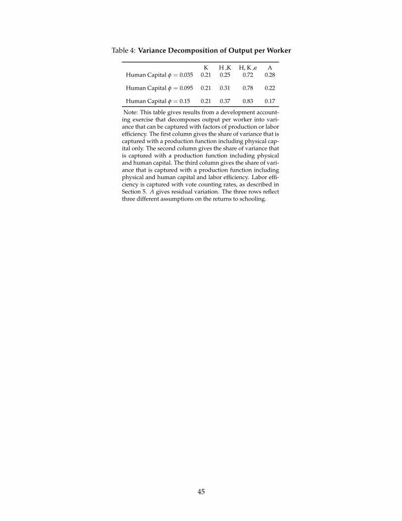
Table 4: Variance Decomposition of Output per Worker

K H ,K H, K ,e AHuman Capital φ = 0.035 0.21 0.25 0.72 0.28

Human Capital φ = 0.095 0.21 0.31 0.78 0.22

Human Capital φ = 0.15 0.21 0.37 0.83 0.17

Note: This table gives results from a development account-ing exercise that decomposes output per worker into vari-ance that can be captured with factors of production or laborefficiency. The first column gives the share of variance that iscaptured with a production function including physical cap-ital only. The second column gives the share of variance thatis captured with a production function including physicaland human capital. The third column gives the share of vari-ance that is captured with a production function includingphysical and human capital and labor efficiency. Labor effi-ciency is captured with vote counting rates, as described inSection 5. A gives residual variation. The three rows reflectthree different assumptions on the returns to schooling.

45

Table 5: Robustness

IQR (%) North-South (%) Dev. Accounting Resid. (%)

Value Added per Worker 0.21 0.20 0.69

Baseline 0.12 0.07 0.22

Election 2013 0.11 0.04 0.06

Referendum April 0.13 0.09 0.42

Referendum December 0.11 0.07 0.19

Controls for # Polling Stations 0.12 0.10 0.25

1-2 Polling stations 0.12 0.08 0.18

Adjusted VCR 0.13 0.08 0.26

Controlled VCR 0.14 0.08 0.39

Note: This table shows robustness of our main results to a variety of specifications. The three columns corre-spond to three main results. The first column gives the difference in output per unit of labor efficiency betweenthe 75 percentile and the 25 percentile province. The second gives the difference in output per worker in the northand south of Italy, if all Provinces in southern Italy had the labor efficiency of the median northern Province. Thethird gives the share of the variance in output per worker that remains unexplained using a production functionusing physical and human capital, and labor efficiency. The first row gives result when labor efficiency is as-sumed equal in all provinces. The second gives our benchmark results, where labor efficiency is measured usingvote counting rates, averaged across the election (using total time) and the two referenda. Rows 3 to 5 give resultswhen labor efficiency is measured separately from each of the three polls. The sixth row pools all three polls onceagain and controls non-parameterically for the number of polling stations, as in Figure A.10. The seventh rowrestricts attention to municipalities with no more than two polling stations. The eighth row uses the AdjustedVCR measure that controls for the complexity of the vote counting task, as described in Table 2. The ninth rowuses the Controlled VCR measure that control for the complexity of the task and for vote counters’ characteristicsin the election, as described in Table 3.

46

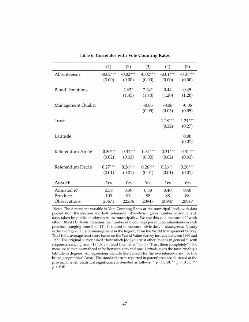
Table 6: Correlates with Vote Counting Rates

(1) (2) (3) (4) (5)

Absenteeism -0.02∗∗∗ -0.02∗∗∗ -0.02∗∗∗ -0.01∗∗∗ -0.01∗∗∗

(0.00) (0.00) (0.00) (0.00) (0.00)

Blood Donations 2.63∗ 2.34∗ 0.44 0.45(1.45) (1.40) (1.20) (1.20)

Management Quality -0.06 -0.06 -0.06(0.05) (0.05) (0.05)

Trust 1.28∗∗∗ 1.24∗∗∗

(0.22) (0.27)

Latitude 0.00(0.01)

Referendum Apr16 -0.30∗∗∗ -0.31∗∗∗ -0.31∗∗∗ -0.31∗∗∗ -0.31∗∗∗

(0.02) (0.02) (0.02) (0.02) (0.02)

Referendum Dec16 0.27∗∗∗ 0.26∗∗∗ 0.26∗∗∗ 0.26∗∗∗ 0.26∗∗∗

(0.01) (0.01) (0.01) (0.01) (0.01)

Area FE Yes Yes Yes Yes Yes

Adjusted R2 0.38 0.39 0.38 0.40 0.40Province 103 93 88 88 88Observations 23671 22286 20947 20947 20947

Note: The dependent variable is Vote Counting Rates at the municipal level, with datapooled from the election and both referenda. Absenteeism gives number of annual sickdays taken by public employees in the municipality. We use this as a measure of “workethic”. Blood Donations measures the number of blood bags per million inhabitants in eachprovince (ranging from 0 to .11). It is used to measure “civic duty”. Management Qualityis the average quality of management in the Region, from the World Management Survey.Trust is the average trust score based on the World Value Survey for Italy between 1990 and1999. The original survey asked “how much [do] you trust other Italians in general?” withresponses ranging from (1) “Do not trust them at all” to (5) “Trust them completely”. Themeasure is then normalized to be between zero and one. Latitude gives the municipality’slatitude in degrees. All regressions include fixed effects for the two referenda and for fivebroad geographical Areas. The standard errors reported in parentheses are clustered at theprovincial level. Statistical significance is denoted as follows: ∗ p < 0.10, ∗∗ p < 0.05, ∗∗∗

p < 0.01

47

Table 7: The Role of Trust in a Contentious Task

(1) (2) (3)

South-Center × Challenged -24.05∗∗∗ -23.39∗∗∗

(7.43) (7.33)

North × Challenged 0.59 1.11(3.20) (2.84)

South-Center × Blank -4.96∗∗∗ -4.21∗∗∗

(0.85) (0.96)

North × Blank -7.86∗∗∗ -7.64∗∗∗

(0.76) (0.93)

South-Center × Invalid -6.09∗∗∗ -4.96∗∗∗

(0.82) (0.89)

North × Invalid -6.47∗∗∗ -5.57∗∗∗

(0.74) (0.73)

Trust 1.50∗∗∗

(0.21)

Challenged -125.56∗∗∗

(42.83)

Challenged × Trust 143.10∗∗∗

(51.99)

North 0.20∗∗∗ 0.21∗∗∗ 0.05(0.04) (0.04) (0.04)

Referendum Apr16 -0.33∗∗∗ -0.52∗∗∗ -0.49∗∗∗

(0.02) (0.02) (0.02)

Referendum Dec16 0.27∗∗∗ 0.04∗∗ 0.07∗∗∗

(0.01) (0.02) (0.02)

Adjusted R2 0.29 0.34 0.37Province 110 110 99Observations 22763 22763 21445

Note: The dependent variable is Vote Counting Rates at the munic-ipal level, with data pooled from the election and both referenda.North and South-Center are dummy variables for municipalities inthe north and south or center of Italy, respectively. Challenged, blank,and invalid are the percent of challenged, blank, and invalid votesin the municipality, respectively. Trust is a survey measure of trust,normalized on a scale from zero to one as described in the footnoteto Table 6. Regressions include fixed effects for both referenda. Thefirst two columns show that challenged votes slow down the votecounting process in the south of Italy but not the north. The thirdcolumn shows that challenged votes slow down the vote countingprocess more where trust is low. The standard errors reported inparentheses are clustered at the provincial level. Statistical signifi-cance is denoted as follows: ∗ p < 0.10, ∗∗ p < 0.05, ∗∗∗ p < 0.01

48

Web Appendix (Not For Publication)

A Appendix: Supplementary Figures & Tables

Figure A.1: Sample Ballots: Election 2013

Panel A: Piemonte

Panel B: Sicily

49

Figure A.2: Sample Ballots: Referenda

Panel A: April 2016

Panel B: December 2016

50

Figu

reA

.3:V

ote

Cou

ntin

g

51

Figu

reA

.4:V

ote

Cou

ntin

gTi

me

and

Rat

esin

the

Apr

il20

16R

efer

endu

m

012345Percent

.51

1.5

22.

53

Tim

e

0246Percent

010

020

030

040

0R

aw V

CR

0246Percent

-2-1

01

Adju

sted

VC

R

Not

e:Th

efig

ure

plot

sth

edi

stri

buti

ons

ofvo

teco

unti

ngti

mes

(top

left

),vo

teco

unti

ngra

tes

(top

righ

t)an

dA

djus

ted

Vote

Cou

ntin

gR

ates

(bot

tom

)in

the

refe

rend

umof

Apr

il20

16.T

head

just

edvo

teco

unti

ngra

tead

just

sfo

rth

eco

mpl

exit

yof

the

vote

coun

ting

task

,rep

orte

din

Tabl

e2.

52

Figu

reA

.5:V

ote

Cou

ntin

gTi

me

and

Rat

esin

the

Sena

teEl

ecti

on20

13

0246Percent

24

68

Tim

e

012345Percent

5010

015

020

025

030

0R

aw V

CR

0246Percent

-1.5

-1-.5

0.5

1Ad

just

ed V

CR

Not

e:T

hefig

ure

plot

sth

edi

stri

buti

ons

ofvo

teco

unti

ngti

mes

(top

left

),vo

teco

unti

ngra

tes

(top

righ

t)an

dA

djus

ted

vote

coun

ting

rate

s(b

otto

m)i

nth

eel

ecti

onof

2013

,usi

ngvo

teco

unti

ngti

mes

inth

ese

nate

.The

adju

sted

vote

coun

ting

rate

adju

sts

for

the

com

plex

ity

ofth

evo

teco

unti

ngta

sk,r

epor

ted

inTa

ble

2.

53

Figu

reA

.6:V

ote

Cou

ntin

gR

ates

and

Val

ueA

dded

Per

Wor

ker

acro

ssIt

alia

nPr

ovin

ces

AG

AL

AN

AO

ARAP

AT

AVBA

BT

BL

BN

BG

BI

BO

BZ

BS

BR

CA

CLCB

CI

CECT

CZ

CH

CO

CS

CR

KR

CN

EN

FM

FEFI

FG

FC

FR

GE

GO

GR

IMIS

AQ

SP

LT

LE

LC

LI

LO

LUM

C

MN

MS

MT

VS

ME

MI

MO

MB

NA

NO

NU

OG

OT

OR

PD

PA

PR

PV

PG

PUPE

PC

PI

PT

PN

PZ

PO

RG

RA

RC

RE

RI

RN

RM

RO

SA

SS

SV

SI

SR

SO TATE

TR

TO

TP

TN

TV

TSUD

VA

VE

VB

VC

VR

VV

VI

VT

33.23.43.63.8VA/worker

-.4-.2

0.2

VCR

Not

e:T

hefig

ure

com

pare

svo

teco

unti

ngra

tes

inth

eel

ecti

onof

2013

wit

hva

lue

adde

dpe

rw

orke

rin

Ital

ian

prov

ince

s.

54

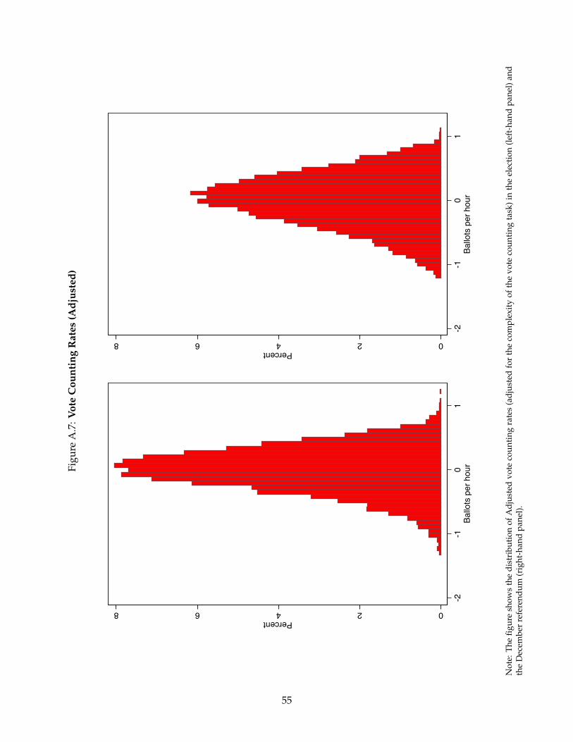
Figu

reA

.7:V

ote

Cou

ntin

gR

ates

(Adj

uste

d)

02468Percent

-2-1

01

Ballo

ts p

er h

our

02468Percent

-2-1

01

Ballo

ts p

er h

our

Not

e:Th

efig

ure

show

sth

edi

stri

buti

onof

Adj

uste

dvo

teco

unti

ngra

tes

(adj

uste

dfo

rth

eco

mpl

exit

yof

the

vote

coun

ting

task

)in

the

elec

tion

(lef

t-ha

ndpa

nel)

and

the

Dec

embe

rre

fere

ndum

(rig

ht-h

and

pane

l).

55

Figu

reA

.8:V

CR

,Adj

uste

dV

CR

,and

Con

trol

led

VC

R

AG

AL

AN

AO

AR

AP

AT

AV

BA

BT

BL

BN

BG

BI

BO

BZ

BS

BR

CA

CL

CB

CI

CE

CT

CZ

CH

CO

CS

CR

KR

CN

EN

FM

FEFI

FG

FC

FR

GE

GO

GR

IM

IS

AQ

SP

LT

LE

LCLI

LOLU

MC

MN

MS

MT

VS

ME

MI

MO

MB

NA

NO

NU

OG

OT

OR

PD

PA

PR

PVPG

PU

PE

PC

PI

PT

PN

PZ

PO

RG

RA

RC

RE

RI

RN

RM

RO

SA

SS

SV

SI

SR

SOTA

TE

TR

TO

TP

TN

TV

TS

UD

VA

VE

VB

VC

VR

VV

VI

VT

-.6-.4-.20.2VCR raw

-.4-.2

0.2

VCR

adju

sted

AG

AL

ANAO

AR

APAT

AV

BA

BL

BN

BG

BIBO

BZBS

CA

CL

CB

CI

CE

CT

CZ

CHCO

CS

CR

CN

EN

FM

FE

FI

FG

FC

FR

GE

GO

GR

IM

IS

AQ

SP

LE

LC

LI

LO

LU

MC

MN

MS

MT

VS

ME

MI

MO

MB

NA

NONU

OT

OR

PD

PA

PR

PV

PG

PU

PE

PC

PI

PT

PN

PZ

PO

RG

RA

RC

RE

RI

RN

RMRO

SA

SS

SV

SI

SR

SO TA

TE

TR

TO

TN

TV

TS

UDVA

VE

VB

VC

VR

VV

VI

VT

-.6-.4-.20.2.4VCR controlled

-.4-.2

0.2

VCR

adju

sted

Not

e:T

hefig

ure

com

pare

sth

ree

mea

sure

sof

vote

coun

ting

rate

s.Th

ele

ft-h

and

pane

lcom

pare

s(r

aw)V

CR

wit

hA

djus

ted

VC

R,w

hich

cont

rols

for

the

com

plex

ity

ofth

evo

teco

unti

ngta

sk.

The

Spea

rman

corr

elat

ion

coef

ficie

ntis

0.98

.Th

eri

ght-

hand

pane

lcom

pare

sC

ontr

olle

dV

CR

and

Adj

uste

dV

CR

,whe

reth

efo

rmer

cont

rols

also

for

vote

-cou

nter

char

acte

rist

ics.

The

Spea

rman

corr

elat

ion

coef

ficie

ntis

0.70

.

56

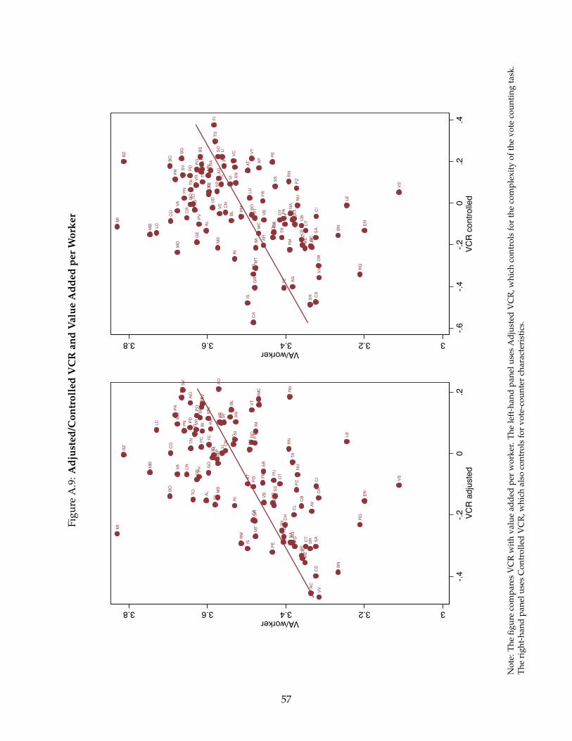
Figu

reA

.9:A

djus

ted/

Con

trol

led

VC

Ran

dV

alue

Add

edpe

rW

orke

r

AG

AL

AN

AO

ARAP

AT

AV

BA

BL

BN

BG

BI

BO

BZ

BS

CA

CLCB

CI

CECT

CZ

CH

CO

CS

CR

CN

EN

FM

FEFI

FG

FC

FR

GE

GO

GR

IM

IS

AQ

SP

LE

LC

LI

LO

LU

MC

MN

MS

MT

VS

ME

MI

MO

MB

NA

NO

NU

OT

OR

PD

PA

PR

PV

PG

PUPE

PC

PI

PT

PN

PZ

PO

RG

RA

RC

RE

RI

RN

RM

RO

SA

SS

SV

SI

SR

SO TA

TETR

TOTN

TV

TSUD

VA

VE

VB

VC

VR

VV

VI

VT

33.23.43.63.8VA/worker

-.4-.2

0.2

VCR

adju

sted

AG

AL

AN

AO

ARAPAT

AV

BA

BL

BN

BG

BIBO

BZ

BS

CA

CLCB

CI

CECT

CZ

CH

CO

CS

CR

CN

EN

FM

FEFI

FG

FC

FR

GE

GO

GR

IM

IS

AQ

SP

LE

LC

LI

LO

LU

MC

MN

MS

MT

VS

ME

MI

MO

MB

NA

NO NU

OT

OR

PD

PA

PR

PV

PG

PUPE

PC

PI

PT

PN

PZ

PO

RG

RA

RC

RE

RI

RN

RM RO

SA

SS

SV

SI

SR

SO

TA

TETR

TOTN

TV

TSUDVA VE

VB

VC

VR

VV

VI

VT

33.23.43.63.8VA/worker

-.6-.4

-.20

.2.4

VCR

cont

rolle

d

Not

e:Th

efig

ure

com

pare

sV

CR

wit

hva

lue

adde

dpe

rw

orke

r.Th

ele

ft-h

and

pane

luse

sA

djus

ted

VC

R,w

hich

cont

rols

for

the

com

plex

ity

ofth

evo

teco

unti

ngta

sk.

The

righ

t-ha

ndpa

nelu

ses

Con

trol

led

VC

R,w

hich

also

cont

rols

for

vote

-cou

nter

char

acte

rist

ics.

57

Figu

reA

.10:

Num

ber

ofPo

llin

gSt

atio

nsan

dV

ote

Cou

ntin

gR

ate

44.555.56log VCR

12

3-5

6-15

16-5

051

-100

>101

# of

pol

ling

stat

ions

Not

e:Th

efig

ure

plot

sth

epa

ram

eter

sfr

oma

regr

essi

onof

vote

coun

ting

rate

son

bins

ofnu

mbe

rof

polli

ngst

atio

ns,w

ith

stan

dard

erro

rssh

own

wit

hw

hisk

ers.

Vote

coun

ting

rate

sdo

n’ta

ppea

rto

beas

soci

ated

wit

hth

enu

mbe

rof

polli

ngst

atio

nsin

am

unic

ipal

ity.

58

Figu

reA

.11:

Con

trol

led

VC

R

02468Percent

-1.5

-1-.5

0.5

1Ba

llots

per

hou

r

02468Percent

-1.5

-1-.5

0.5

1Ba

llots

per

hou

r

Not

e:Th

efig

ure

plot

svo

teco

unti

ngra

tes

usin

gto

talt

ime

(lef

t-ha

ndpa

nel)

and

Sena

teti

me

(rig

ht-h

and

pane

l)in

the

2013

elec

tion

,aft

erco

ntro

lling

fort

heco

mpl

exit

yof

the

vote

coun

ting

task

and

vote

coun

ters

’cha

ract

eris

tics

.

59

Tabl

eA

.1:R

epre

sent

ativ

enes

sof

Surv

eySa

mpl

eof

Vot

eC

ount

erC

hara

cter

isti

cs

Surv

eyed

Mun

icip

alit

ies

All

Mun

icip

alit

ies

Mea

nSD

Min

Max

Mea

nSD

Min

Max

Nor

thW

est

VC

R21

8.5

68.5

61.5

396.

620

2.0

68.3

60.3

397.

5#

Polli

ngSt

atio

ns6.

331

.81

653

5.1

31.8

112

48N

orth

East

VC

R23

8.4

67.6

83.5

397.

623

4.0

66.3

63.0

397.

5#

Polli

ngSt

atio

ns7.

215

.91

187

8.5

23.7

144

5C

ente

rV

CR

213.

965

.982

.136

5.4

193.

261

.660

.637

9.2

#Po

lling

Stat

ions

8.6

14.8

110

312

.490

.01

2600

Sout

han

dIs

land

sV

CR

151.

147

.661

.131

8.3

153.

746

.460

.537

0.8

#Po

lling

Stat

ions

5.8

8.5

171

8.9

28.7

188

6

Not

e:Th

eta

ble

com

pare

svo

teco

unti

ngra

tes

and

the

num

ber

ofpo

lling

stat

ions

inm

unic

ipal

itie

sth

atre

spon

ded

toou

rsu

rvey

onvo

teco

unte

rch

arac

teri

stic

san

din

allm

unic

ipal

itie

s.Th

efo

urro

ws

corr

espo

ndto

four

mac

roar

eas

ofth

eco

untr

y.Th

esa

mpl

eap

pear

sre

pres

enta

tive

inte

rms

ofm

unic

ipal

ity

size

and

vote

coun

ting

prod

ucti

vity

.

60

Table A.2: Vote Counting Rates and Complexity of the Vote Counting Task: Referenda

Referendum - April 2016 Referendum - December 2016

(1) (2) (3) (4) (5) (6)

Challenged 3.47 3.67 4.57 -18.07 -21.59 -19.07(2.89) (2.80) (3.35) (19.14) (18.72) (20.86)

Blank -6.91∗∗∗ -6.55∗∗∗ -4.62∗∗∗ -13.30∗∗∗ -17.76∗∗∗ -12.61∗∗∗

(1.10) (1.06) (1.09) (2.94) (2.24) (2.03)

Invalid -9.13∗∗∗ -8.89∗∗∗ -6.87∗∗∗ -5.76∗∗∗ -5.81∗∗∗ -5.27∗∗∗

(0.90) (0.95) (0.78) (0.78) (0.73) (0.76)

Yes vote share 0.21 0.79∗∗∗ 0.72∗∗∗ 0.20(0.26) (0.23) (0.11) (0.14)

Adjusted R2 0.07 0.07 0.07 0.03 0.05 0.03Province 110 110 103 110 110 103Observations 7589 7589 3331 7585 7585 3321

Note: The dependent variable is the log of Vote Counting Rates (VCRi,s) for election s and munici-pality i as defined in equation (1). In the first three columns, VCR is measured for the Referendumof April 2016 . In the last three columns VCR is measured for the Referendum of December 2016.Columns three and six include only municipalities with no more than two polling stations. Chal-lenged is the share of challenged ballots. Blank is the share of ballots that were left blank. Invalid isthe share of ballots that were deemed incompatible with the voting procedure. Yes vote share is thepercentage of votes in favour of "YES". The standard errors reported in parentheses are clusteredat the provincial level. Statistical significance is denoted as follows: ∗ p < 0.10, ∗∗ p < 0.05, ∗∗∗

p < 0.01

61

B Data Appendix

B.1 Vote counting data

Vote counting data and the vote counting process are described in the main text. They were ob-

tained from the Ministry of Interior.

B.2 Value Added Per Worker in Firms

The data spans the period 2006-2013 and is downloaded from ORBIS database of Bureau van Dijk.

We construct the average across these years for 110 provinces in Italy. The variables are measured

in thousand EUR at 2010 prices. The Italian CPI index was obtained from EUROSTAT.

Value added per worker

Our value added measure is the sum of average cost of employee33 and profit per employee.

We drop the observations with negative values.

Capital per worker

Following Gopinath et al. (2015), we construct the capital stock as the sum of tangible fixed

assets and intangible fixed assets. We drop observations with negative values for intangible fixed

assets and observations with negative or zero values for tangible fixed assets.34 We also delete

firm-year observations where the ratio of tangible fixed assets to total assets is greater than one.

We then divide the capital stock of the firm with number of employees.

Winsorization

We winsorize at the 1st and 99th percentile the variables average cost of employee, profit per

employee, tangible fixed assets and intangible fixed assets. We also drop capital per worker values

that are above the 99th percentile.

33Average cost of employee and profit per employee are under Global ratios/industrial companies/per employee ratios inthe database.

34For 2006 total assets were unavaialble, so we didn’t drop observations with tangible assets that are larger than totalassets. Tangible and intangible capital values are under Global standard format/industrial companies/balance sheet in thedatabase.

62

From Output per Worker in the Average Firm to Average Output per Worker

We also compute a weighted average measure, where weight of each firm in the province is its

employment share in that province35.

Industry Control

In order to control for the differences that could arise from industry decomposition across

provinces, we run the following regression:

ValueAdded f = β0 + β1i Industryi + β2jProvincej + ε f

where ValueAdded f is the value added of the firm, and Industry and Province are dummy

variables to capture the fixed effects. Then, value added for each province is the sum of intercept,

province fixed effect and industry fixed effect adjusted with its frequency in Italy:

ValueAddedcf = β0 + ∑ β1i fi + β2jProvincej

Trimmed Sample

We trimmed the sample with respect to turnover (last available year) to control for distribution

of firms across provinces. We exclude the firms that are in the top 10, 20 and 50 percentiles. We

use the first of these in our main specification, but results are robust to using the other two and the

untrimmed sample.

Consistent Sample

We restrict attention to the subset of firms for which both Capital per worker and VA per

worker can be calculated. Per year around 20% of the firm observations are dropped due to lack

of matched data.35Number of employees are under Key financials&employees in the database

63

B.3 Survey on Vote Counter Characteristics

The data on vote counters (presidenti, segretari and scrutatori), consists of a cross-section with a

single observation per individual involved in the vote counting process during the Italian general

election on 24-25 February 2013. It was collected directly from inidividual municipalities.

First e-mail data request

We obtained a list of the e-mail addresses of 7,533 municipalities from the National Association

of Italian Comuni (ANCI).

Between April 18, 2016 and April 22, 2016, we contacted every address in the list using an auto-

mated e-mail. We asked them to indicate, for every individual involved in the counting process:

1. Role (presidente, segretario and scrutatore);

2. Birthplace;

3. Birthdate;

4. Gender;

5. Highest degree earned;

6. Occupation;

7. For Presidents: whether they had served as polling station president in the past..

Residence is know as vote counters can only be appointed in their town of residence. Finally,

we also asked the municipality to indicate whether the vote counters were drawn randomly or

selected by the electoral committee.

The initial response was underwhelming. It is impossible to quantify how many of the addresses

in our list were outdated and in how many cases the e-mail was just ignored. In many cases mu-

nicipalities refused our request, directed us to a higher official, or requested further information.

Second e-mail data request

In the hope of increasing the response rate, we decided to rewrite the content of the e-mail

(asking for the same set of data) and run a second round from the April 27 to April 29, sending

7,157 emails to all those that had not yet replied.

64

The second e-mail was more successful. We believe this effect is partially due to increasing the

salience of the first request. In total, we were able to collect data on 1,456 of the 8,093 Italian

municipalities that existed in 2013. It is worth noting that since some municipalities have been

aggregated into larger entities since then, in a few cases a single reply provided data on more than

one municipality. A total of 179 municipalities refused to share data because of administrative

cost, privacy concerns, or data unavailability. An additional 188 municipalities replied expressing

willingness to share the data but have shared the data to date

Age variables

We computed the exact age at the time of the election using date of birth.

Education variables

The information on the highest degree earned was used to calculate years of schooling.

Employment status variables

Occupational data was used to determine whether vote counters were employed, self-employed,

students, unemployed or out of the labor force. Given the large number of students in the sample,

we employed two additional definitions of student, to ensure that this category was not misused.

In the first we restrict students to be younger than 29; in the second we exclude individuals older

than 29 or, alternately, that did not complete upper-secondary school.

We used the resulting individual level variables to compute municipal and provincial average

characteristics of the scrutatori.

65