lable at ScienceDirect

Building and Environment 81 (2014) 320e333

Contents lists avai

Building and Environment

journal homepage: www.elsevier .com/locate/bui ldenv

Measuring the dynamics of contrast & daylight variability inarchitecture: A proof-of-concept methodology

Siobhan Rockcastle*, Marilyne AndersenInterdisciplinary Laboratory of Performance-Integrated Design (LIPID), School of Architecture, Civil and Environmental Engineering (ENAC), EcolePolytechnique F�ed�erale de Lausanne (EPFL), Lausanne, Switzerland

a r t i c l e i n f o

Article history:Received 17 April 2014Received in revised form28 May 2014Accepted 12 June 2014Available online 25 June 2014

Keywords:Daylighting designSpatial contrastLight variabilityVisual effectsDynamic lightingLighting perception

* Corresponding author.E-mail addresses: Siobhan.rockcastle@epfl.ch, s

(S. Rockcastle), marilyne.andersen@epfl.ch (M. Ander

http://dx.doi.org/10.1016/j.buildenv.2014.06.0120360-1323/© 2014 Elsevier Ltd. All rights reserved.

a b s t r a c t

Unlike artificial light sources, which can be calibrated to meet a desired luminous effect regardless oflatitude, climate, or time of day, daylight is a dynamic light source, which produces variable shadowpatterns and fluctuating levels of brightness. While we know that perceptual impacts of daylight such ascontrast and temporal variability are important factors in architectural design, we are left with animbalanced set of performance indicators e and few, if any, which address the positive visual andtemporal qualities of daylight from an occupant point-of-view. If visual characteristics of daylight, suchas contrast and spatial compositions, can be objectively measured, we can contribute to a more holisticanalysis of daylit architecture with metrics that complement existing illumination and comfort-basedperformance criteria. Using image processing techniques, this paper will propose a proof-of-conceptmethodology for quantifying contrast-based visual effects within renderings of daylit architecture.Two new metrics will be proposed; annual spatial contrast and annual luminance variability. Using 56time-step instances (taken symmetrically from across the day and year) this paper will introduce amethod for quantifying local contrast values within a set of rendered images and plot those instancesover time to visualize hourly and seasonal fluctuations in contrast composition. Using the same 56 in-stances, this paper will also introduce a method for quantifying variations in luminance (brightness)between instances to measure fluctuations in brightness. This paper pre-validates each of the proposedmethods by calculating annual spatial contrast and annual luminance variability across ten abstractdigital models and comparing those results to the authors' own intuitive ranking.

© 2014 Elsevier Ltd. All rights reserved.

1. Introduction

Daylight offers both functional and aesthetic value to architec-ture, providing natural and energy-efficient illumination for inte-rior tasks and infusing interior space with light, shadow, andtexture. Unlike artificial light sources, which can be adjusted tomeet a desired luminous effect regardless of latitude, climate, ortime of day; daylight is sensitive to a number of dynamic condi-tions. The latitude of a given location affects the length and in-tensity of daylight hours across the year while climatic factors affectits strength and variability on an hourly scale. These variable con-ditions result in a highly dynamic source of illumination andperceptual phenomena. While many architects have expressed theimportance of these phenomenological effects on our perception of

iobhan.rockcastle@gmail.comsen).

space [1e4] we are left with disproportionally few, if any, daylightdesign metrics that can evaluate the positive impacts of luminousvariability within the visual field.

A preoccupationwith electricity consumption, brought about bythe oil crisis of the 1970s and strengthened through contemporarytrends in energy conservation, encourages architects and engineersto place value in daylight as an energy-efficient alternative toartificial light. In an effort to reduce energy consumption,daylighting research has gravitated toward the widespread devel-opment of task-based illumination metrics [5] as a means of off-setting a building's reliance on electric light. Visual comfortmetrics, especially those pertaining to glare, have also gainedpredominance within the last two decades, as the emphasis ondaylight integration has led to an increase in glazed facades andcomplex shading systems that can trigger occupant discomfortduring visual tasks. Advances in computational power have helpedto facilitate time-intensive simulations, allowing us to transitionfrom point-in-time glare risk-assessment to dynamic annual met-rics [6,7]. Perceptual performance indicators such as contrast and

S. Rockcastle, M. Andersen / Building and Environment 81 (2014) 320e333 321

variability, on the other hand, are traditionally defined as qualita-tive design factors and quantitative methods to explore theirimpact or relevance have been limited. Although subjective in na-ture, the perceptual performance of space is central to architecturaldesign and often ranks above other more concrete evaluationcriteria (like task-plane illuminance and visual comfort) within thedesign process. With this in mind, it is important to considerperceptual performance criteria alongside illumination and visualcomfort metrics to develop a more holistic evaluation of daylight inarchitecture. A brief review of existing daylight performance met-rics will help situate this paper and underline the need for newmetrics that address the positive impacts of daylight within ourfield-of-view.

1.1. Task-driven performance metrics

The most common daylight metrics used today typically focuson task performance, whether in regard to illumination (work-plane task illumination) or to visual comfort (eye-level glare eval-uation). A third, less established category, but one of particularrelevance to this paper, relates occupant preferences to perceptualfactors such as brightness and luminous diversity within anestablished view position.

Over the past several decades, there have been significant im-provements in our understanding of daylight as a dynamic andvariable source of illumination. We have transitioned from staticmetrics such as Daylight Factor DF [8] to annual climate-basedmetrics like Daylight Autonomy DA [5] or Useful Daylight Illumi-nance UDI [9], as well as Acceptable Illuminance Extent AIE [10]when dealing with whole areas of interest over time, that all ac-count for a more statistically accurate method of quantifying in-ternal illuminance levels [11]. While DF may be the mostwidespread task-based illumination metric currently used inpractice, it limits our understanding of daylight as a dynamic sourceof illumination, assuming a more-is-better attitude regardless ofthe sky type or intended programmatic use of the space underconsideration [5]. Dynamic illumination metrics, such as DA, UDI orAIE, can evaluate annual illumination thresholds, taking into ac-count building orientation and climate-driven sky type to provide amore accurate assessment of task-plane illuminance.

Unlike task-based illumination metrics that rely on illuminance,visual comfort metrics (typically pertaining to glare) tend to rely onluminance [12]. Of the four photometric quantities (luminous flux,intensity, illuminance, and luminance), luminance is most closelyrelated to how the eye perceives light, and as such, appears as theonly quantity capable of expressing visual discomfort. As lumi-nance, brightness, and contrast are subjectively evaluated, methodsto analyze glare discomfort are fragmented across no less thanseven established metrics [7,13,14]. While these indices do not al-ways agree, partly due to the fact that some were developed forelectric lighting sources and others for daylight, most are derivedfrom the same four quantities: luminance, size of glare sources,position of glare source, and the surrounding field of luminancethat the eye must adapt to [15]. Glare-based visual comfort metrics,such as Daylight Glare Probability DGP [7], considered the mostreliable index for side-lit office spaces under daylight conditions,have also evolved into dynamic annual metrics such as DGPs [15]which provides a comprehensive yearly analysis of glare, withlimited computational intensity [6].

Task-driven illumination metrics such as DF and DA can be usedto determine whether an interior space is sufficiently illuminatedfor the performance of visual tasks, whereas comfort-based lumi-nance metrics such as DGP allow us to evaluate the visual field forsources of glare-based discomfort. While the shift toward climate-based metrics such as DA and UDI represents a significant

improvement in daylight analysis, this data is limited to a two-dimensional task-surface and does not correspond to the three-dimensional view of space that is perceived by an occupant.Although dynamic glare metrics such as DGPs evaluate a three-dimensional view position, they also only establish that highlevels of contrast negatively impact visual comfort. Of the manyestablished glare indices, not one addresses the notion of contrastas a positive visual effect.

Furthermore, task-driven illumination and visual comfort met-rics are only applicable in spaces where visual tasks are frequentlycarried out. For spaces where visual tasks are less indicative oflighting performance, we have few, if any, broadly accepted metricsto help guide designers. In the absence of quantitative criteria, ar-chitects are tasked with creating acceptably bright or visuallyengaging environments, based on subjective criteria [16]. For manyarchitects, this task is made difficult by the dynamic nature ofsunlight and the challenges associated with predicting the range ofvisual effects that will occur across the day and year.

1.2. Perceptual daylight metrics

Two factors that are widely accepted to impact the field-of-viewindaylit architecture are average luminanceand luminancevariation[17]. The former has been directly associated with perceived light-ness and the latter with visual interest [18]. To evaluate the visualimpacts of luminosity within interior architecture, existing researchhas relied on average luminance or “brightness,” threshold lumi-nance, and luminance variation (or standard deviation) in line withoccupant surveys to establish trends in preference. Survey-basedstudies most commonly rely on high-dynamic-range HDR images,digital photographs or renderings produced through Radiance,which provide an expanded range of photometric information,allowing us to evaluate characteristics such as brightness andcontrast [19,20]. Some studies have found that bothmean luminanceand luminance variationwithin an office environment contribute tooccupant preference [21], whereas others have discovered thatluminance distribution across an occupant's field-of-view [22] aswell as the strength of variation are factors of preference [23].

In a study conducted by Cetegen et al., the authors discovered apositive trend between increased average luminance levels andsatisfaction for the view in an office setting, but they also saw atrend between increased luminance diversity and the participant'simpression of excitement [21]. In a second study, also conductedin an office setting, Tiller and Veitch concluded that a non-uniform lighting distribution increased an occupant's perceptionof brightness and preference [22]. Along the same lines, Wyme-lenberg & Inanici conducted a study on occupant preferences to-ward light distribution in an office setting with horizontal blinds.The authors of the study concluded that adequate variations inluminance tended to create a stimulating visual environment,while excessive variability tended to create uncomfortable spaces[23].

The problemwith those studies that rely on average luminance,luminance range, and standard deviation, is that they do notaddress the spatial diversity of luminance values within an occu-pants' field-of-view. In a daylight classification system proposed byClaude Demers, she categorizes digital images of architecture interms of average brightness and standard deviation. While thismethod produces a typological language to codify lighting ambi-ance, she acknowledges that it cannot account for the spatial dis-tribution of perceived light, which is central to the visualexperience of architecture [24]. To address the importance of lightdistribution, Parpairi et al. developed the Luminance Difference(LD) index, which proposes a spatially dependent method formeasuring luminance diversity across a selected view direction.

S. Rockcastle, M. Andersen / Building and Environment 81 (2014) 320e333322

This method relies on eye-level luminance measurements tocalculate the difference in luminance levels across a range ofacceptable angles corresponding to eye and headmovement [25]. Astudy, which calculates the LD index across three selected viewpositions, found that luminance variability was highly appreciatedby the participants and that variability rather than intensity werefound to contribute to occupant satisfaction. While the LD indexproposes a method for analyzing the spatial diversity of luminancevalues across an occupant's point-of-view, it does not address thetemporal impacts of these visual effects. Furthermore, the methodrelies on physical measurements in live space, which can pose anumber of practical problems, such as the movement of people andthe disruption of equipment over extended studies.

In summary, existing research has produced promising in-dications that both luminance distribution and diversity play animportant role in an occupant's perception of and preference to-ward the luminous environment. At the same time, we have yet tosee an informative method for measuring the spatial diversity ofluminance values across a human perspective, nor have we seen amethod for quantifying the temporal impacts of daylight vari-ability throughout the year. While most studies attempt to extractpreference trends from luminance data, this paper seeks toestablish a comparative framework and method for evaluatinghow contrasted or variable a scene may appear (over space andover time). While future research might explore the connectionbetween contrast, variability, and human preferences toward lightdistribution, the authors believe that any evaluation of suchperceived qualities must be based on specific design objectives. Inother words, there are no definitive values for contrast or vari-ability that necessarily indicate a ‘good’ or ‘bad’ set of visualperformance criteria, but rather there might be a range of valuesthat are recommended for the intended usage of a given space(such as a museum or office). These recommended values must beflexible enough to accommodate the designer's intent, whileproving appropriate for the completion of any occupant tasks. Asthe composition of luminance is dynamic within daylit architec-ture, the authors of this paper will propose a new class of metricsthat can quantify these perceptual effects over time. Buildingupon the author's thesis project at the Massachusettes Institute ofTechnology, this paper will introduce two new metrics; annualspatial contrast and annual luminance variability [44,45]. Usingcase study spaces to pre-validate results for each of the proposedmetrics in a relative gradient from high to low, this paper willestablish a methodology for comparing spatial contrast andluminance variability between spaces that are similar in size andorientation. As human preferences toward daylight are dependenton the intended program of an architectural space (i.e. its uses),this comparative framework will provide architects with a base-line against which design variations can be compared andperceptual qualities of daylight can be contextualized.

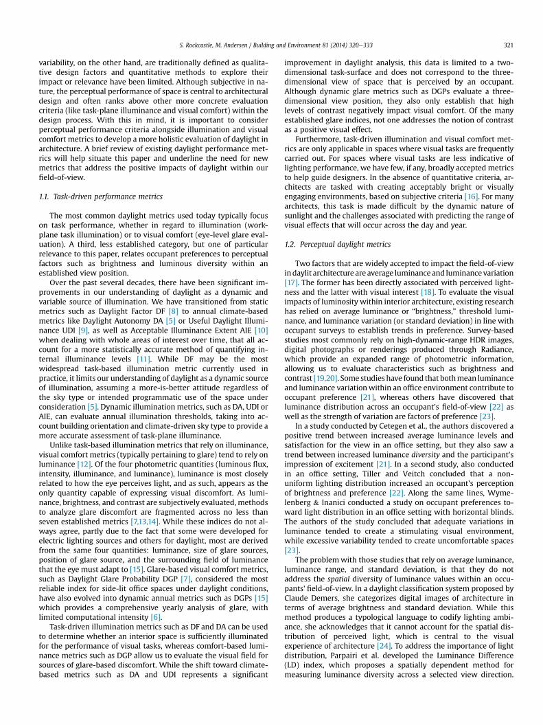
Fig. 1. Two abstract renderings that differ in composition, but share

2. Measuring contrast through digital images

In image analysis, there are two types of measures that arecommonly used to quantify contrast: those that rely on globalmeasures and those that rely on local measures. Global measuresmost often rely on two single points of extreme brightness anddarkness, taking into account the difference in maximum andminimum luminance values [26]. Other methods account foraverage luminance values, rather than extremes [27], and thestandard deviation of image chroma (i.e. color channels) andlightness [28]. While these global contrast measures provide asingle comprehensible value, they cannot effectively predictperceived contrast between two images that vary in composition[29].

Local contrast measures were developed to overcome the limi-tations associated with global measures by quantifying the effect ofcomposition on contrasting areas of brightness and darkness.Included within this group of measures are methods that measurespatial frequencies in the Fourier domain [30], those that measure aweighted color contrast based on the distance between chromaregions [31], and those that calculate the difference between asingle pixel and a surrounding region or neighborhood [32,33].Despite this range of methods, there is still little consensus on howto produce a single number that represents the contrast perceptionof an image through localized pixel or neighborhood values [29].On the one hand, a single number cannot easily distinguish be-tween two images that vary in composition. This is due to the lossof information that occurs between a matrix of values or a powerspectrum (resulting from a Fourier transformation) and the finalvalue, which is often a mean or median value. On the other hand, asingle number is a compact measure that can be compared tosubjective experiments, which often produce a single value fromoccupant surveys.

For example, if we compare two renderings of daylit spaces side-by-side (Fig. 1) and relied on existing methods of global contrast-analysis, such as mean brightness or standard deviation, we wouldnot be able to differentiate between the two images despite theirvaried compositions. The image on the left (Fig. 1a) shows a densepattern of light and shadow - with a mean brightness of 120 and astandard deviation of 18. The image on the right (Fig. 1b) containslarger patches of sunlight, but has a similar mean brightness of 132and standard deviation of 22. The obvious drawback to measure-ments like average luminance and standard deviation, is the loss ofinformation that occurs when individual values are removed fromthe spatial framework of their composition.

As was discussed in Section 1.2, existing studies that addresscontrast perception within daylit architecture have focused onglobal measures such as standard deviation, luminance range, andaverage luminance, due to the ease of comparing single globalmeasures against subjective rankings [23,24]. Given the lack of

similar values for mean pixel brightness and standard deviation.

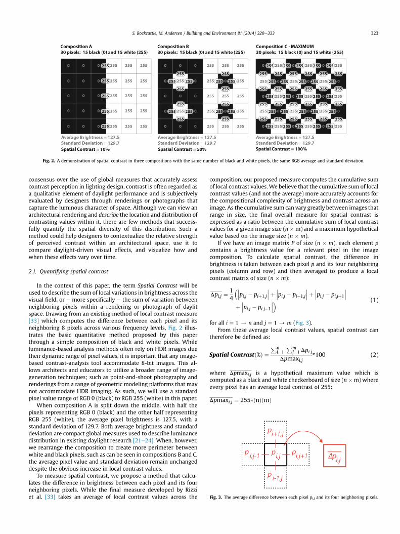
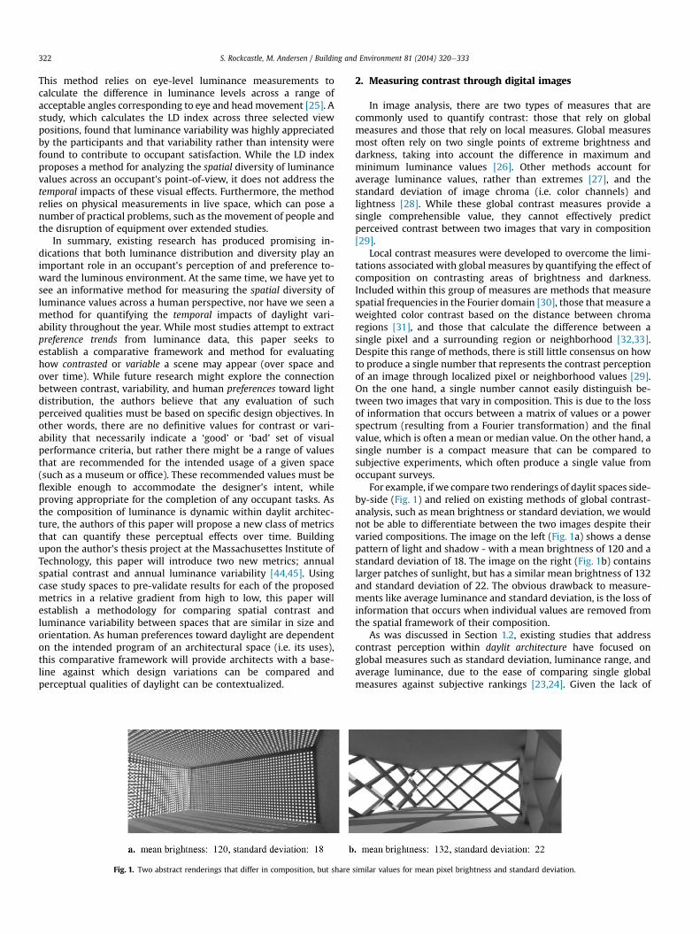
Fig. 2. A demonstration of spatial contrast in three compositions with the same number of black and white pixels, the same RGB average and standard deviation.

Fig. 3. The average difference between each pixel pi,j and its four neighboring pixels.

S. Rockcastle, M. Andersen / Building and Environment 81 (2014) 320e333 323

consensus over the use of global measures that accurately assesscontrast perception in lighting design, contrast is often regarded asa qualitative element of daylight performance and is subjectivelyevaluated by designers through renderings or photographs thatcapture the luminous character of space. Although we can view anarchitectural rendering and describe the location and distribution ofcontrasting values within it, there are few methods that success-fully quantify the spatial diversity of this distribution. Such amethod could help designers to contextualize the relative strengthof perceived contrast within an architectural space, use it tocompare daylight-driven visual effects, and visualize how andwhen these effects vary over time.

2.1. Quantifying spatial contrast

In the context of this paper, the term Spatial Contrast will beused to describe the sum of local variations in brightness across thevisual field, or e more specifically e the sum of variation betweenneighboring pixels within a rendering or photograph of daylitspace. Drawing from an existing method of local contrast measure[33] which computes the difference between each pixel and itsneighboring 8 pixels across various frequency levels, Fig. 2 illus-trates the basic quantitative method proposed by this paperthrough a simple composition of black and white pixels. Whileluminance-based analysis methods often rely on HDR images duetheir dynamic range of pixel values, it is important that any image-based contrast-analysis tool accommodate 8-bit images. This al-lows architects and educators to utilize a broader range of image-generation techniques; such as point-and-shoot photography andrenderings from a range of geometric modeling platforms that maynot accommodate HDR imaging. As such, we will use a standardpixel value range of RGB 0 (black) to RGB 255 (white) in this paper.

When composition A is split down the middle, with half thepixels representing RGB 0 (black) and the other half representingRGB 255 (white), the average pixel brightness is 127.5, with astandard deviation of 129.7. Both average brightness and standarddeviation are compact global measures used to describe luminancedistribution in existing daylight research [21e24]. When, however,we rearrange the composition to create more perimeter betweenwhite and black pixels, such as can be seen in compositions B and C,the average pixel value and standard deviation remain unchangeddespite the obvious increase in local contrast values.

To measure spatial contrast, we propose a method that calcu-lates the difference in brightness between each pixel and its fourneighboring pixels. While the final measure developed by Rizziet al. [33] takes an average of local contrast values across the

composition, our proposed measure computes the cumulative sumof local contrast values. We believe that the cumulative sum of localcontrast values (and not the average) more accurately accounts forthe compositional complexity of brightness and contrast across animage. As the cumulative sum can vary greatly between images thatrange in size, the final overall measure for spatial contrast isexpressed as a ratio between the cumulative sum of local contrastvalues for a given image size (n � m) and a maximum hypotheticalvalue based on the image size (n � m).

If we have an image matrix P of size (n � m), each element pcontains a brightness value for a relevant pixel in the imagecomposition. To calculate spatial contrast, the difference inbrightness is taken between each pixel p and its four neighboringpixels (column and row) and then averaged to produce a localcontrast matrix of size (n � m):

Dpi;j ¼14

����pi;j � piþ1;j

���þ���pi;j � pi�1;j

���þ���pi;j � pi;jþ1

���þ���pi;j � pi;j�1

���� (1)

for all i ¼ 1 / n and j ¼ 1 / m (Fig. 3).From these average local contrast values, spatial contrast can

therefore be defined as:

Spatial Contrastð%Þ ¼Pn

i¼1Pm

j¼1 Dpi;jDpmaxi;j

*100 (2)

where Dpmaxi;j is a hypothetical maximum value which iscomputed as a black and white checkerboard of size (n �m) whereevery pixel has an average local contrast of 255:

Dpmaxi;j ¼ 255�ðnÞðmÞ

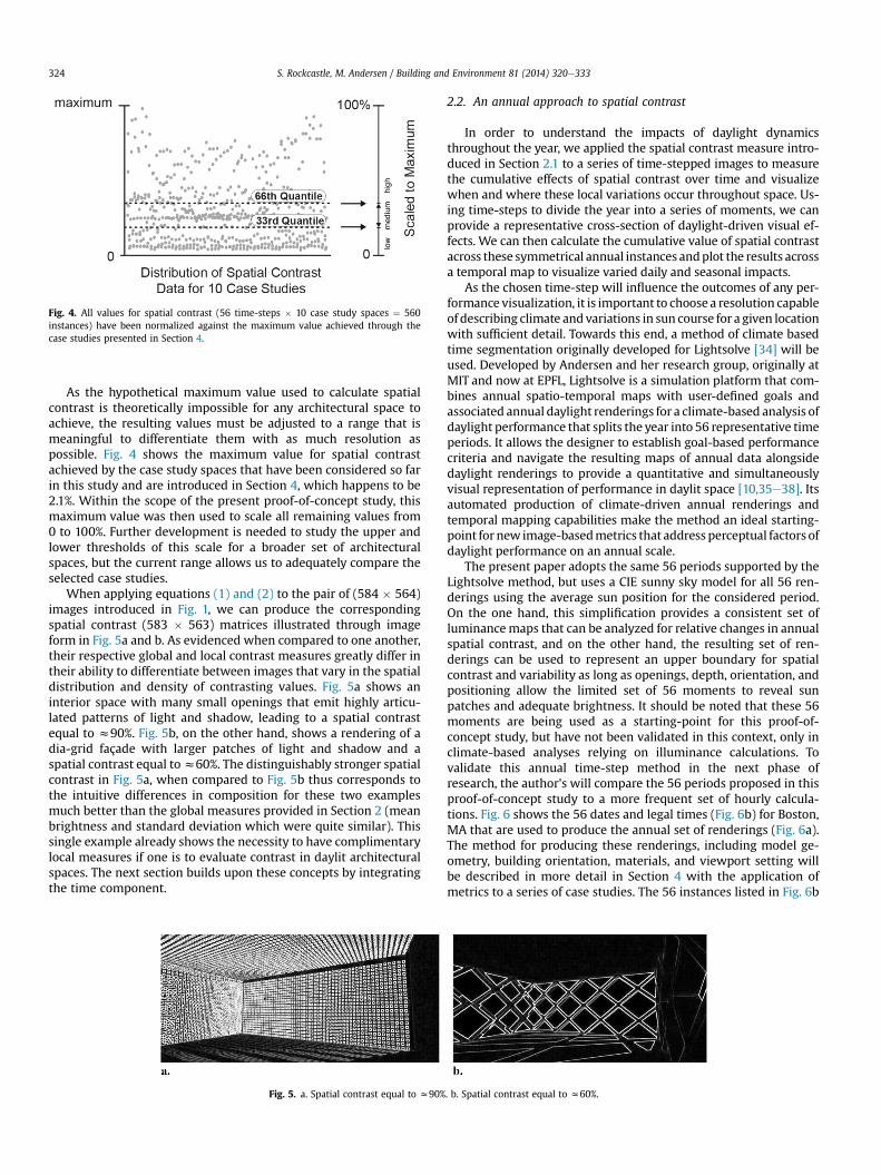
Fig. 4. All values for spatial contrast (56 time-steps � 10 case study spaces ¼ 560instances) have been normalized against the maximum value achieved through thecase studies presented in Section 4.

S. Rockcastle, M. Andersen / Building and Environment 81 (2014) 320e333324

As the hypothetical maximum value used to calculate spatialcontrast is theoretically impossible for any architectural space toachieve, the resulting values must be adjusted to a range that ismeaningful to differentiate them with as much resolution aspossible. Fig. 4 shows the maximum value for spatial contrastachieved by the case study spaces that have been considered so farin this study and are introduced in Section 4, which happens to be2.1%. Within the scope of the present proof-of-concept study, thismaximum value was then used to scale all remaining values from0 to 100%. Further development is needed to study the upper andlower thresholds of this scale for a broader set of architecturalspaces, but the current range allows us to adequately compare theselected case studies.

When applying equations (1) and (2) to the pair of (584 � 564)images introduced in Fig. 1, we can produce the correspondingspatial contrast (583 � 563) matrices illustrated through imageform in Fig. 5a and b. As evidenced when compared to one another,their respective global and local contrast measures greatly differ intheir ability to differentiate between images that vary in the spatialdistribution and density of contrasting values. Fig. 5a shows aninterior space with many small openings that emit highly articu-lated patterns of light and shadow, leading to a spatial contrastequal to z90%. Fig. 5b, on the other hand, shows a rendering of adia-grid façade with larger patches of light and shadow and aspatial contrast equal toz60%. The distinguishably stronger spatialcontrast in Fig. 5a, when compared to Fig. 5b thus corresponds tothe intuitive differences in composition for these two examplesmuch better than the global measures provided in Section 2 (meanbrightness and standard deviation which were quite similar). Thissingle example already shows the necessity to have complimentarylocal measures if one is to evaluate contrast in daylit architecturalspaces. The next section builds upon these concepts by integratingthe time component.

Fig. 5. a. Spatial contrast equal to z90%

2.2. An annual approach to spatial contrast

In order to understand the impacts of daylight dynamicsthroughout the year, we applied the spatial contrast measure intro-duced in Section 2.1 to a series of time-stepped images to measurethe cumulative effects of spatial contrast over time and visualizewhen and where these local variations occur throughout space. Us-ing time-steps to divide the year into a series of moments, we canprovide a representative cross-section of daylight-driven visual ef-fects. We can then calculate the cumulative value of spatial contrastacross these symmetrical annual instances andplot the results acrossa temporal map to visualize varied daily and seasonal impacts.

As the chosen time-step will influence the outcomes of any per-formance visualization, it is important to choose a resolution capableof describing climate andvariations in sun course for a given locationwith sufficient detail. Towards this end, a method of climate basedtime segmentation originally developed for Lightsolve [34] will beused. Developed by Andersen and her research group, originally atMIT and now at EPFL, Lightsolve is a simulation platform that com-bines annual spatio-temporal maps with user-defined goals andassociated annual daylight renderings for a climate-based analysis ofdaylight performance that splits the year into 56 representative timeperiods. It allows the designer to establish goal-based performancecriteria and navigate the resulting maps of annual data alongsidedaylight renderings to provide a quantitative and simultaneouslyvisual representation of performance in daylit space [10,35e38]. Itsautomated production of climate-driven annual renderings andtemporal mapping capabilities make the method an ideal starting-point for new image-basedmetrics that address perceptual factors ofdaylight performance on an annual scale.

The present paper adopts the same 56 periods supported by theLightsolve method, but uses a CIE sunny sky model for all 56 ren-derings using the average sun position for the considered period.On the one hand, this simplification provides a consistent set ofluminancemaps that can be analyzed for relative changes in annualspatial contrast, and on the other hand, the resulting set of ren-derings can be used to represent an upper boundary for spatialcontrast and variability as long as openings, depth, orientation, andpositioning allow the limited set of 56 moments to reveal sunpatches and adequate brightness. It should be noted that these 56moments are being used as a starting-point for this proof-of-concept study, but have not been validated in this context, only inclimate-based analyses relying on illuminance calculations. Tovalidate this annual time-step method in the next phase ofresearch, the author's will compare the 56 periods proposed in thisproof-of-concept study to a more frequent set of hourly calcula-tions. Fig. 6 shows the 56 dates and legal times (Fig. 6b) for Boston,MA that are used to produce the annual set of renderings (Fig. 6a).The method for producing these renderings, including model ge-ometry, building orientation, materials, and viewport setting willbe described in more detail in Section 4 with the application ofmetrics to a series of case studies. The 56 instances listed in Fig. 6b

. b. Spatial contrast equal to z60%.

Fig. 6. a. 56 Annual renderings of a hypothetical top-lit space. b. Dates and times of the 56 instances selected to represent a symmetrical annual cross-section (all times are legal andnot solar).

S. Rockcastle, M. Andersen / Building and Environment 81 (2014) 320e333 325

will be used to produce all annual sets of renderings used for visualanalysis in this paper.

In order to calculate annual spatial contrast, instantaneousspatial contrast is computed across all 56moments shown in Fig. 6a.The cumulative sum of these instances, shown in Fig. 7a, highlightsthe location and strength of spatial contrast throughout the year,revealing areas that receive consistently high (red) and low (blue)contrast. In order to visualize when these dynamic effects of spatialcontrast vary throughout the year, the sum of spatial contrast foreach of the 56 renderings is plotted temporally to express the fre-quency andmagnitude of daily and seasonal variations (Fig. 7b). Thevertical axis of the temporal map shows daylight hours, from sun-rise to sunset, while the horizontal axis shows days of the year, fromJanuary 1st to December 31st. Values are given a color scale to showrelative strength from low to high, which has been adjusted toaccommodate appropriate minimum and maximum values asdetermined by the case studies that will be introduced in Section 4.

Fig. 7. Annual spatial contrast results for a top-lit space. a. Cumulative annua

3. Measuring variability in daylit space

The second metric presented by this paper attempts to providea measure of the annual variation in luminance values across aselected view. Whereas spatial contrast identifies compositionalcontrast boundaries between pixels within an image, and annualspatial contrast maps the accumulation of those contrast bound-aries over time, annual luminance variability accounts for thecumulative difference in pixel values as they vary from onemoment to the next. This metric is useful in describing the in-tensity of variation that occurs across a space as a combination ofboth time and dynamic natural lighting conditions. Many spacesthat measure low in spatial contrast may still display moderate-to-high amounts of luminance variability, as the brightnessthroughout a space can transform dramatically over the course oftime while still maintaining a smooth compositional gradient inbrightness.

l map of luminance variability. b. Temporal map of luminance variability.

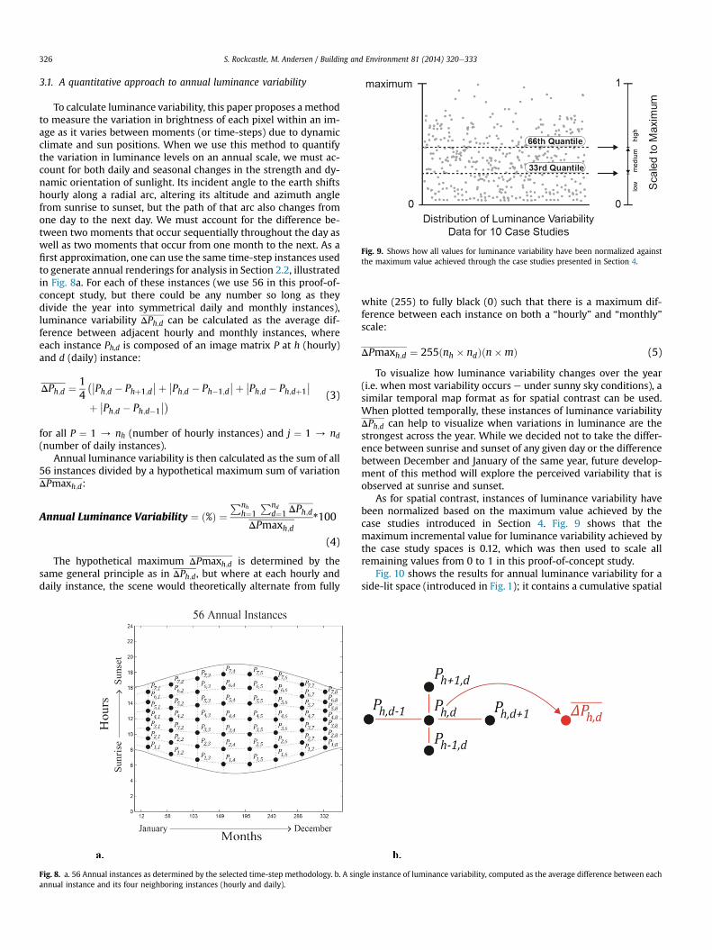
Fig. 9. Shows how all values for luminance variability have been normalized againstthe maximum value achieved through the case studies presented in Section 4.

S. Rockcastle, M. Andersen / Building and Environment 81 (2014) 320e333326

3.1. A quantitative approach to annual luminance variability

To calculate luminance variability, this paper proposes a methodto measure the variation in brightness of each pixel within an im-age as it varies between moments (or time-steps) due to dynamicclimate and sun positions. When we use this method to quantifythe variation in luminance levels on an annual scale, we must ac-count for both daily and seasonal changes in the strength and dy-namic orientation of sunlight. Its incident angle to the earth shiftshourly along a radial arc, altering its altitude and azimuth anglefrom sunrise to sunset, but the path of that arc also changes fromone day to the next day. We must account for the difference be-tween two moments that occur sequentially throughout the day aswell as two moments that occur from one month to the next. As afirst approximation, one can use the same time-step instances usedto generate annual renderings for analysis in Section 2.2, illustratedin Fig. 8a. For each of these instances (we use 56 in this proof-of-concept study, but there could be any number so long as theydivide the year into symmetrical daily and monthly instances),luminance variability DPh;d can be calculated as the average dif-ference between adjacent hourly and monthly instances, whereeach instance Ph,d is composed of an image matrix P at h (hourly)and d (daily) instance:

DPh;d ¼ 14���Ph;d � Phþ1;d

��þ ��Ph;d � Ph�1;d��þ ��Ph;d � Ph;dþ1

��þ ��Ph;d � Ph;d�1

���(3)

for all P ¼ 1 / nh (number of hourly instances) and j ¼ 1 / nd(number of daily instances).

Annual luminance variability is then calculated as the sum of all56 instances divided by a hypothetical maximum sum of variationDPmaxh;d:

Annual Luminance Variability ¼ ð%Þ ¼Pnh

h¼1Pnd

d¼1 DPh;dDPmaxh;d

*100

(4)

The hypothetical maximum DPmaxh;d is determined by thesame general principle as in DPh;d, but where at each hourly anddaily instance, the scene would theoretically alternate from fully

Fig. 8. a. 56 Annual instances as determined by the selected time-step methodology. b. A sinannual instance and its four neighboring instances (hourly and daily).

white (255) to fully black (0) such that there is a maximum dif-ference between each instance on both a “hourly” and “monthly”scale:

DPmaxh;d ¼ 255ðnh � ndÞðn�mÞ (5)

To visualize how luminance variability changes over the year(i.e. when most variability occurs e under sunny sky conditions), asimilar temporal map format as for spatial contrast can be used.When plotted temporally, these instances of luminance variabilityDPh;d can help to visualize when variations in luminance are thestrongest across the year. While we decided not to take the differ-ence between sunrise and sunset of any given day or the differencebetween December and January of the same year, future develop-ment of this method will explore the perceived variability that isobserved at sunrise and sunset.

As for spatial contrast, instances of luminance variability havebeen normalized based on the maximum value achieved by thecase studies introduced in Section 4. Fig. 9 shows that themaximum incremental value for luminance variability achieved bythe case study spaces is 0.12, which was then used to scale allremaining values from 0 to 1 in this proof-of-concept study.

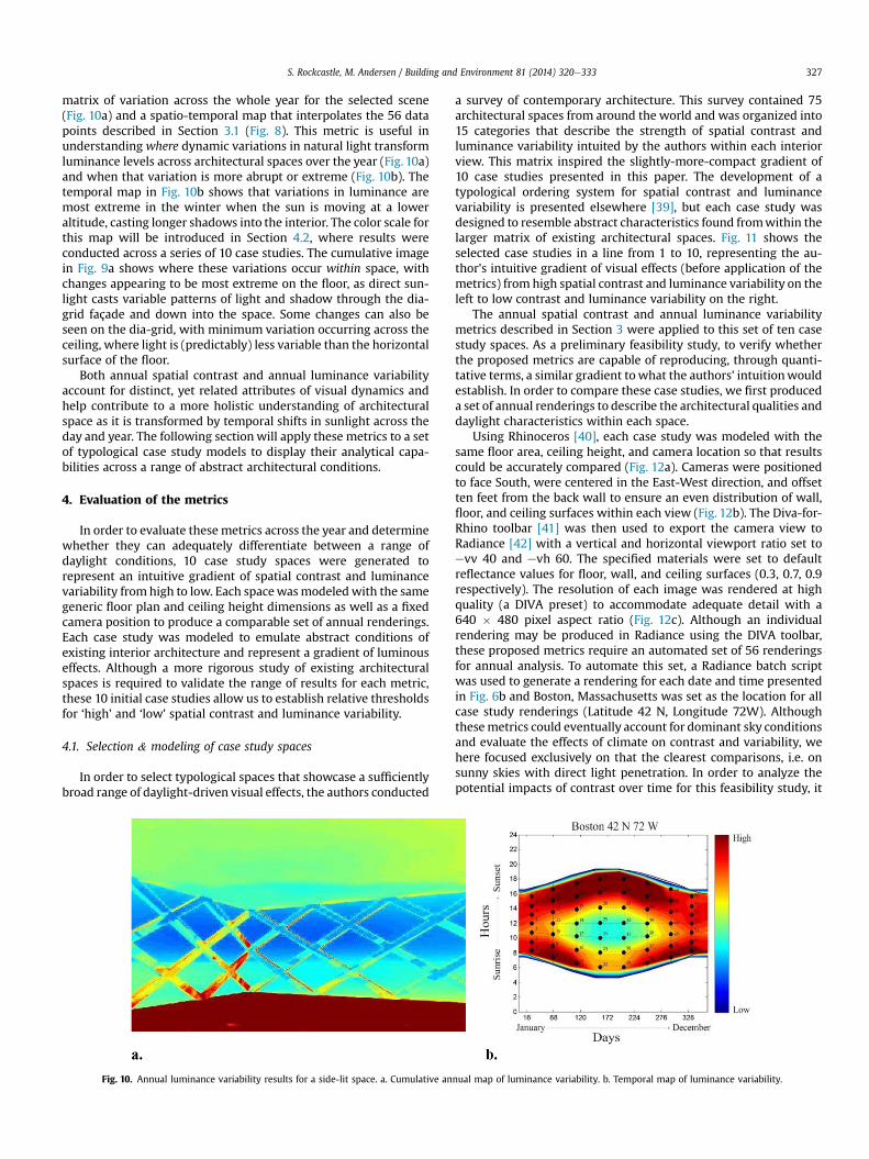
Fig. 10 shows the results for annual luminance variability for aside-lit space (introduced in Fig. 1); it contains a cumulative spatial

gle instance of luminance variability, computed as the average difference between each

S. Rockcastle, M. Andersen / Building and Environment 81 (2014) 320e333 327

matrix of variation across the whole year for the selected scene(Fig. 10a) and a spatio-temporal map that interpolates the 56 datapoints described in Section 3.1 (Fig. 8). This metric is useful inunderstanding where dynamic variations in natural light transformluminance levels across architectural spaces over the year (Fig. 10a)and when that variation is more abrupt or extreme (Fig. 10b). Thetemporal map in Fig. 10b shows that variations in luminance aremost extreme in the winter when the sun is moving at a loweraltitude, casting longer shadows into the interior. The color scale forthis map will be introduced in Section 4.2, where results wereconducted across a series of 10 case studies. The cumulative imagein Fig. 9a shows where these variations occur within space, withchanges appearing to be most extreme on the floor, as direct sun-light casts variable patterns of light and shadow through the dia-grid façade and down into the space. Some changes can also beseen on the dia-grid, with minimum variation occurring across theceiling, where light is (predictably) less variable than the horizontalsurface of the floor.

Both annual spatial contrast and annual luminance variabilityaccount for distinct, yet related attributes of visual dynamics andhelp contribute to a more holistic understanding of architecturalspace as it is transformed by temporal shifts in sunlight across theday and year. The following sectionwill apply these metrics to a setof typological case study models to display their analytical capa-bilities across a range of abstract architectural conditions.

4. Evaluation of the metrics

In order to evaluate these metrics across the year and determinewhether they can adequately differentiate between a range ofdaylight conditions, 10 case study spaces were generated torepresent an intuitive gradient of spatial contrast and luminancevariability fromhigh to low. Each spacewasmodeledwith the samegeneric floor plan and ceiling height dimensions as well as a fixedcamera position to produce a comparable set of annual renderings.Each case study was modeled to emulate abstract conditions ofexisting interior architecture and represent a gradient of luminouseffects. Although a more rigorous study of existing architecturalspaces is required to validate the range of results for each metric,these 10 initial case studies allow us to establish relative thresholdsfor ‘high’ and ‘low’ spatial contrast and luminance variability.

4.1. Selection & modeling of case study spaces

In order to select typological spaces that showcase a sufficientlybroad range of daylight-driven visual effects, the authors conducted

Fig. 10. Annual luminance variability results for a side-lit space. a. Cumulative an

a survey of contemporary architecture. This survey contained 75architectural spaces from around the world and was organized into15 categories that describe the strength of spatial contrast andluminance variability intuited by the authors within each interiorview. This matrix inspired the slightly-more-compact gradient of10 case studies presented in this paper. The development of atypological ordering system for spatial contrast and luminancevariability is presented elsewhere [39], but each case study wasdesigned to resemble abstract characteristics found fromwithin thelarger matrix of existing architectural spaces. Fig. 11 shows theselected case studies in a line from 1 to 10, representing the au-thor's intuitive gradient of visual effects (before application of themetrics) from high spatial contrast and luminance variability on theleft to low contrast and luminance variability on the right.

The annual spatial contrast and annual luminance variabilitymetrics described in Section 3 were applied to this set of ten casestudy spaces. As a preliminary feasibility study, to verify whetherthe proposed metrics are capable of reproducing, through quanti-tative terms, a similar gradient towhat the authors' intuitionwouldestablish. In order to compare these case studies, we first produceda set of annual renderings to describe the architectural qualities anddaylight characteristics within each space.

Using Rhinoceros [40], each case study was modeled with thesame floor area, ceiling height, and camera location so that resultscould be accurately compared (Fig. 12a). Cameras were positionedto face South, were centered in the East-West direction, and offsetten feet from the back wall to ensure an even distribution of wall,floor, and ceiling surfaces within each view (Fig. 12b). The Diva-for-Rhino toolbar [41] was then used to export the camera view toRadiance [42] with a vertical and horizontal viewport ratio set toevv 40 and evh 60. The specified materials were set to defaultreflectance values for floor, wall, and ceiling surfaces (0.3, 0.7, 0.9respectively). The resolution of each image was rendered at highquality (a DIVA preset) to accommodate adequate detail with a640 � 480 pixel aspect ratio (Fig. 12c). Although an individualrendering may be produced in Radiance using the DIVA toolbar,these proposed metrics require an automated set of 56 renderingsfor annual analysis. To automate this set, a Radiance batch scriptwas used to generate a rendering for each date and time presentedin Fig. 6b and Boston, Massachusetts was set as the location for allcase study renderings (Latitude 42 N, Longitude 72W). Althoughthesemetrics could eventually account for dominant sky conditionsand evaluate the effects of climate on contrast and variability, wehere focused exclusively on that the clearest comparisons, i.e. onsunny skies with direct light penetration. In order to analyze thepotential impacts of contrast over time for this feasibility study, it

nual map of luminance variability. b. Temporal map of luminance variability.

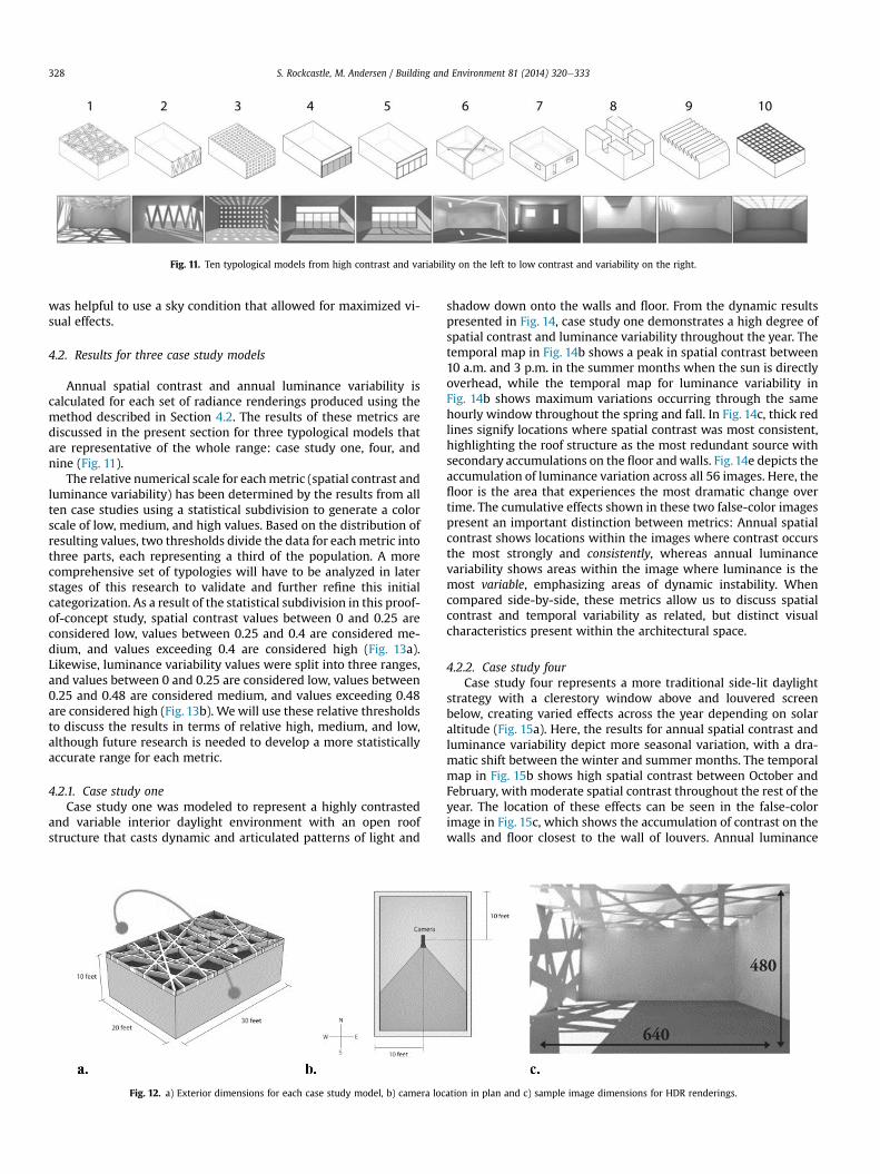
Fig. 11. Ten typological models from high contrast and variability on the left to low contrast and variability on the right.

S. Rockcastle, M. Andersen / Building and Environment 81 (2014) 320e333328

was helpful to use a sky condition that allowed for maximized vi-sual effects.

4.2. Results for three case study models

Annual spatial contrast and annual luminance variability iscalculated for each set of radiance renderings produced using themethod described in Section 4.2. The results of these metrics arediscussed in the present section for three typological models thatare representative of the whole range: case study one, four, andnine (Fig. 11).

The relative numerical scale for eachmetric (spatial contrast andluminance variability) has been determined by the results from allten case studies using a statistical subdivision to generate a colorscale of low, medium, and high values. Based on the distribution ofresulting values, two thresholds divide the data for eachmetric intothree parts, each representing a third of the population. A morecomprehensive set of typologies will have to be analyzed in laterstages of this research to validate and further refine this initialcategorization. As a result of the statistical subdivision in this proof-of-concept study, spatial contrast values between 0 and 0.25 areconsidered low, values between 0.25 and 0.4 are considered me-dium, and values exceeding 0.4 are considered high (Fig. 13a).Likewise, luminance variability values were split into three ranges,and values between 0 and 0.25 are considered low, values between0.25 and 0.48 are considered medium, and values exceeding 0.48are considered high (Fig. 13b). Wewill use these relative thresholdsto discuss the results in terms of relative high, medium, and low,although future research is needed to develop a more statisticallyaccurate range for each metric.

4.2.1. Case study oneCase study one was modeled to represent a highly contrasted

and variable interior daylight environment with an open roofstructure that casts dynamic and articulated patterns of light and

Fig. 12. a) Exterior dimensions for each case study model, b) camera loc

shadow down onto the walls and floor. From the dynamic resultspresented in Fig. 14, case study one demonstrates a high degree ofspatial contrast and luminance variability throughout the year. Thetemporal map in Fig. 14b shows a peak in spatial contrast between10 a.m. and 3 p.m. in the summer months when the sun is directlyoverhead, while the temporal map for luminance variability inFig. 14b shows maximum variations occurring through the samehourly window throughout the spring and fall. In Fig. 14c, thick redlines signify locations where spatial contrast was most consistent,highlighting the roof structure as the most redundant source withsecondary accumulations on the floor andwalls. Fig. 14e depicts theaccumulation of luminance variation across all 56 images. Here, thefloor is the area that experiences the most dramatic change overtime. The cumulative effects shown in these two false-color imagespresent an important distinction between metrics: Annual spatialcontrast shows locations within the images where contrast occursthe most strongly and consistently, whereas annual luminancevariability shows areas within the image where luminance is themost variable, emphasizing areas of dynamic instability. Whencompared side-by-side, these metrics allow us to discuss spatialcontrast and temporal variability as related, but distinct visualcharacteristics present within the architectural space.

4.2.2. Case study fourCase study four represents a more traditional side-lit daylight

strategy with a clerestory window above and louvered screenbelow, creating varied effects across the year depending on solaraltitude (Fig. 15a). Here, the results for annual spatial contrast andluminance variability depict more seasonal variation, with a dra-matic shift between the winter and summer months. The temporalmap in Fig. 15b shows high spatial contrast between October andFebruary, with moderate spatial contrast throughout the rest of theyear. The location of these effects can be seen in the false-colorimage in Fig. 15c, which shows the accumulation of contrast on thewalls and floor closest to the wall of louvers. Annual luminance

ation in plan and c) sample image dimensions for HDR renderings.

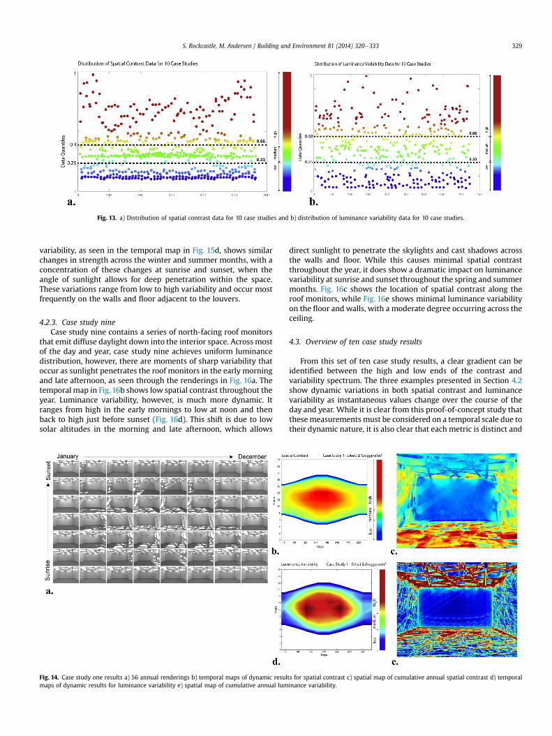
Fig. 13. a) Distribution of spatial contrast data for 10 case studies and b) distribution of luminance variability data for 10 case studies.

S. Rockcastle, M. Andersen / Building and Environment 81 (2014) 320e333 329

variability, as seen in the temporal map in Fig. 15d, shows similarchanges in strength across the winter and summer months, with aconcentration of these changes at sunrise and sunset, when theangle of sunlight allows for deep penetration within the space.These variations range from low to high variability and occur mostfrequently on the walls and floor adjacent to the louvers.

4.2.3. Case study nineCase study nine contains a series of north-facing roof monitors

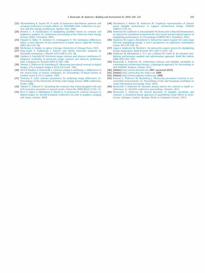
that emit diffuse daylight down into the interior space. Across mostof the day and year, case study nine achieves uniform luminancedistribution, however, there are moments of sharp variability thatoccur as sunlight penetrates the roof monitors in the early morningand late afternoon, as seen through the renderings in Fig. 16a. Thetemporal map in Fig. 16b shows low spatial contrast throughout theyear. Luminance variability, however, is much more dynamic. Itranges from high in the early mornings to low at noon and thenback to high just before sunset (Fig. 16d). This shift is due to lowsolar altitudes in the morning and late afternoon, which allows

Fig. 14. Case study one results a) 56 annual renderings b) temporal maps of dynamic resulmaps of dynamic results for luminance variability e) spatial map of cumulative annual lum

direct sunlight to penetrate the skylights and cast shadows acrossthe walls and floor. While this causes minimal spatial contrastthroughout the year, it does show a dramatic impact on luminancevariability at sunrise and sunset throughout the spring and summermonths. Fig. 16c shows the location of spatial contrast along theroof monitors, while Fig. 16e shows minimal luminance variabilityon the floor and walls, with a moderate degree occurring across theceiling.

4.3. Overview of ten case study results

From this set of ten case study results, a clear gradient can beidentified between the high and low ends of the contrast andvariability spectrum. The three examples presented in Section 4.2show dynamic variations in both spatial contrast and luminancevariability as instantaneous values change over the course of theday and year. While it is clear from this proof-of-concept study thatthesemeasurements must be considered on a temporal scale due totheir dynamic nature, it is also clear that each metric is distinct and

ts for spatial contrast c) spatial map of cumulative annual spatial contrast d) temporalinance variability.

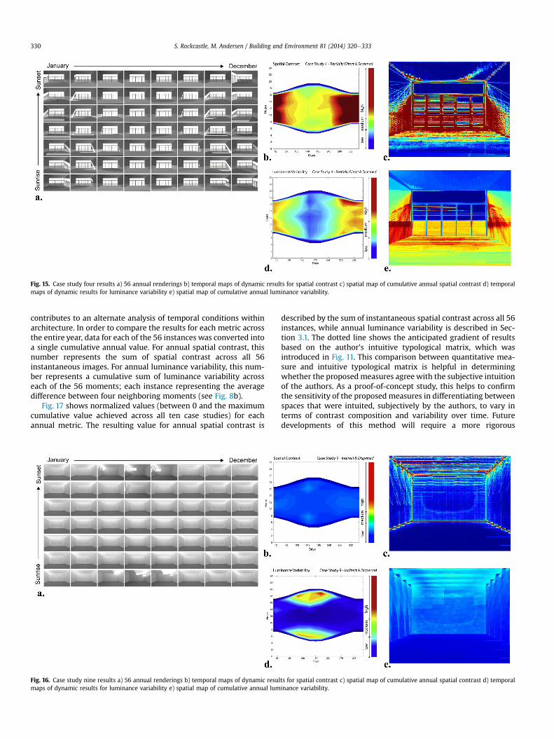
Fig. 15. Case study four results a) 56 annual renderings b) temporal maps of dynamic results for spatial contrast c) spatial map of cumulative annual spatial contrast d) temporalmaps of dynamic results for luminance variability e) spatial map of cumulative annual luminance variability.

S. Rockcastle, M. Andersen / Building and Environment 81 (2014) 320e333330

contributes to an alternate analysis of temporal conditions withinarchitecture. In order to compare the results for each metric acrossthe entire year, data for each of the 56 instances was converted intoa single cumulative annual value. For annual spatial contrast, thisnumber represents the sum of spatial contrast across all 56instantaneous images. For annual luminance variability, this num-ber represents a cumulative sum of luminance variability acrosseach of the 56 moments; each instance representing the averagedifference between four neighboring moments (see Fig. 8b).

Fig. 17 shows normalized values (between 0 and the maximumcumulative value achieved across all ten case studies) for eachannual metric. The resulting value for annual spatial contrast is

Fig. 16. Case study nine results a) 56 annual renderings b) temporal maps of dynamic resumaps of dynamic results for luminance variability e) spatial map of cumulative annual lum

described by the sum of instantaneous spatial contrast across all 56instances, while annual luminance variability is described in Sec-tion 3.1. The dotted line shows the anticipated gradient of resultsbased on the author's intuitive typological matrix, which wasintroduced in Fig. 11. This comparison between quantitative mea-sure and intuitive typological matrix is helpful in determiningwhether the proposedmeasures agree with the subjective intuitionof the authors. As a proof-of-concept study, this helps to confirmthe sensitivity of the proposed measures in differentiating betweenspaces that were intuited, subjectively by the authors, to vary interms of contrast composition and variability over time. Futuredevelopments of this method will require a more rigorous

lts for spatial contrast c) spatial map of cumulative annual spatial contrast d) temporalinance variability.

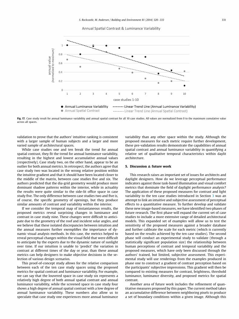
Fig. 17. Case study result for annual luminance variability and annual spatial contrast for all 10 case studies. All values are normalized from 0 to the maximum cumulative valueacross all spaces.

S. Rockcastle, M. Andersen / Building and Environment 81 (2014) 320e333 331

validation to prove that the authors' intuitive ranking is consistentwith a larger sample of human subjects and a larger and morevaried sample of architectural spaces.

While case studies one and ten break the trend for annualspatial contrast, they fit the trend for annual luminance variability,resulting in the highest and lowest accumulative annual values(respectively). Case study two, on the other hand, appear to be anoutlier for both annual metrics. In retrospect, the authors agree thatcase study two was located in the wrong relative position withinthe intuitive gradient and that it should have been located closer tothe middle of the matrix, between case studies five and six. Theauthors predicted that the dia-grid geometry would produce moredominant shadow patterns within the interior, while in actualitythe results were quite similar to the side-lit office space in casestudy five. The only difference between case studies two and five is,of course, the specific geometry of openings, but they producesimilar amounts of contrast and variability within the interior.

If we consider the temporal map of instantaneous results, theproposed metrics reveal surprising changes in luminance andcontrast in case study nine. These changes were difficult to antici-pate due to the geometry of the roof and incident solar angles, andwe believe that these isolated discrepancies between intuition andthe annual measures further exemplifies the importance of dy-namic visual analysis methods. In this case, the metrics helped toreveal perceptual changes within the visual field that were difficultto anticipate by the experts due to the dynamic nature of sunlightover time. If our intuition is unable to ‘predict’ the variation incontrast at different times of the day or year, than these annualmetrics can help designers to make objective decisions in the se-lection of various design scenarios.

This proof-of-concept study allows for the relative comparisonbetween each of the ten case study spaces using the proposedmetrics for spatial contrast and luminance variability. For example,we can say that the louvered space in case study six represents arelatively high degree of both annual spatial contrast and annualluminance variability, while the screened space in case study fourshows a high degree of annual spatial contrast with a low degree ofannual luminance variability. These numbers also allow us tospeculate that case study one experiences more annual luminance

variability than any other space within the study. Although theproposed measures for each metric require further development,these pre-validation results demonstrate the capabilities of annualspatial contrast and annual luminance variability in quantifying arelative set of qualitative temporal characteristics within daylitarchitecture.

5. Discussion & future work

This research raises an important set of issues for architects anddaylight designers. How do we leverage perceptual performanceindicators against those task-based illumination and visual comfortmetrics that dominate the field of daylight performance analysis?The application of these proposed measures for contrast and lightvariability to the ten case studies introduced in Section 3 was anattempt to link an intuitive and subjective assessment of perceptualeffects to a quantitative measure. To further develop and validatethese new image-basedmeasures, we have identified two phases offuture research. The first phase will expand the current set of casestudies to include a more extensive range of detailed architecturalmodels. This expanded set of examples will allow us to test thesensitivity of the proposed measures against a broader databaseand further calibrate the scale for each metric (which is currentlybased on the results achieved by the ten case studies). The secondphase will conduct an experimental study to validate (through astatistically significant population size) the relationship betweenhuman perceptions of contrast and temporal variability and theproposed measures, which have only been discussed through theauthors' trained, but limited, subjective assessment. This experi-mental study will use renderings from the examples produced inphase one to construct a gradient of contrast perception based onthe participants' subjective impressions. This gradient will then becompared to existing measures for contrast, brightness, thresholdluminance, luminance diversity, and proposed metrics for spatialcontrast.

Another area of future work includes the refinement of quan-titative measures proposed by this paper. The current method takesan accumulative difference between neighboring pixels to producea set of boundary conditions within a given image. Although this

S. Rockcastle, M. Andersen / Building and Environment 81 (2014) 320e333332

accounts for a fine level of detail in local luminance variation, themeasure is dependent on pixel density and does not account forlarger regions of contrast that may be perceived by the human eye.A broader look into the cognitive sciences and digital image pro-cessing techniques may produce a more holistic approach toquantifying spatial contrast. Furthermore, the selection of 56annual time-steps must be studied to determine whether theyrepresent an adequate frequency to measure the effects of contrastand variability on a dynamic scale. While this method has beenvalidated for task-based illumination metrics, it has not been vali-dated in this context, and must be compared to an hourly time-stepcalculation to find an appropriate frequency of hourly and dailyinstances.

Additionally, it would be useful to consider the impacts of coloron the perception of contrast and perceptual dynamics in daylitarchitecture. In a study conducted by Simone et al., they concludedthat colored images were often rated higher in perceived contrastthan their greyscale counterparts [43]. As the color temperature ofdaylight varies due to sky conditions, orientation, and time of day, itwould be interesting to consider the influence of color andbrightness on our perception of contrast and light variability.

Ultimately, it is important to propose the integration of thesemetrics into a software package so that perceptual performancemay be measured alongside task-based illumination, visual com-fort, and health-based metrics to provide a more holistic evaluationof daylit space. The Lightsolve project, created at MIT and currentlyunder development at EPFL, proposes an adaptation of these met-rics alongside non-visual and dynamic comfort metrics as part of anintegrated tool to assess human needs in daylit architecture [35].Through an integration task-based metrics for illumination andvisual comfort, photobiological metrics for health, and perceptualfield-of-view metrics like spatial contrast and luminance vari-ability, the designer will be able to fine-tune his/her analysis to fitindividualized performance criteria specific to climate, architec-tural program, and design intent.

6. Conclusion

This paper began with a review of existing daylight analysismetrics to establish the need for new performance criteria that canaccount for the range of perceptual and temporal qualities foundwithin architectural space. These qualities, if measureable, couldthen be positioned alongside existing task-based illuminance andvisual comfort metrics to provide a more holistic analysis ofdaylight performance in architecture. To contextualize theseperceptual and temporal qualities within the discipline of archi-tecture, the authors conducted a survey and produced a typologicalmatrix of daylighting design strategies based on an intuitiveassessment of each space [39]. This typological study revealed adiverse range of daylight-driven visual effects and was used toformalize a set of qualities within each space that contributed to theauthors' subjective assessment. Using this intuitive matrix ascontext, this paper then proposed two new metrics: annual spatialcontrast and annual luminance variability which attempt to mea-sure the effects of spatial and temporal diversity of daylight in ar-chitecture through time-stepped renderings.

In order to measure the intuitive effects described above, HDRrenderings were used to record luminance levels within a selectedview and then compressed down into 8-bit images, providing acompact range of values that could be analyzed. Although spatialcontrast looks at the variation between neighboring pixel valueswithin a selected image, annual spatial contrast and luminancevariability account for the dynamics of contrast and variations inbrightness throughout the year. Through an analysis of an annualset of images (56 renderings that represent an even subdivision of

daylit hours across the year; 7 daily and 8 monthly) the designercan identify the magnitude of spatial contrast and luminancevariability over time and visualize these dynamic effects through acombination of accumulative spatial images and annual temporalmaps. When applied to the ten case study spaces introduced inSection 4, each proposed measure produced a trend in relation tothe author's intuitive ranking, which serves as a pre-validation inthis proof-of-concept study. When compared to existing daylightperformance metrics such as daylight factor, daylight autonomy,and daylight glare probability; these new annual, image-basedmetrics provide important quantitative information about the dy-namic perceptual effects of daylight that have been previouslyunexplored.

These new annual metrics communicate information about thespatial and temporal quality of daylit, providing architects with atool for comparing the magnitude of visual effects within archi-tecture. The implications of this work are widespread, from asimple analytical tool for describing dynamic daylight conditions,to an objective approach that challenges the use of task-basedillumination and visual comfort metrics in a variety of program-matic conditions. By establishing an intuitive gradient of visualeffects and producing a method for quantifying those effects overtime, we are able to re-focus the discussion on daylight perfor-mance to include those perceptual qualities of light that are oftendisregarded in contemporary practice.

References

[1] Holl S. Luminosity/porosity. Tokyo: Toto; 2006.[2] Zumthor P. Atmospheres: architectural environments e surrounding objects.

Basel: Birkh€auser; 2006.[3] Pallasmaa J. The eyes of the skin: architecture and the senses. West Sussex:

Wiley & Sons; 2012.[4] Steane MA, Steemers K. Environmental diversity in architecture. New York:

Spoon Press; 2004.[5] Reinhart C, Mardaljevic JRZ. Dynamic daylight performance metrics for sus-

tainable building design. Leukos 2006;3(1):1e25.[6] Jakubiec J, Reinhart C. The ‘Adaptive Glare Zone’ e a concept for assessing

discomfort glare through daylit spaces. Light Res Technol 2012;44(2):149e70.[7] Wienold J, Christofferson J. Evaluating methods and development of a new

glare prediction model for 152 daylight environments with the use of CCDcameras. Energy Build 2006;38(7):743e57.

[8] Moon P, Spencer D. Illumination for a non-uniform sky. Illum Eng1942;37(10):797e826.

[9] Nabil A, Mardaljevic J. The useful daylight illuminance paradigm: a replace-ment for daylight factors. Energy Build 2006;38(7):905e13.

[10] Kleindienst S, Andersen M. Comprehensive annual daylight design through agoal-based approach. Build Res Inform 2012;40(2):154e73.

[11] Mardaljevic J. Simulation of annual daylighting profiles for internal illumi-nance. Light Res Technol 2000;32(3):111e8.

[12] CIE. Commission Internationale de l'Eclairage Proceedings. Cambridge: Cam-bridge University Press; 1926.

[13] IESNA. IESNA lighting handbook: reference and application. New York: Illu-minating Engineering Society of North America; 2000.

[14] Osterhaus W. Discomfort glare assessment and prevention for daylight ap-plications in office environments. Sol Energy 2005;79(2):140e58.

[15] Wienold J. Dynamic daylight glare evaluation. In: Proceedings of InternationalIBPSA Conference, Glasgow; 2009.

[16] Cuttle C. Towards the third stage of the lighting profession. Light Res Technol2010;42(1):73e93.

[17] Veitch J, Newsham G. Preferred luminous conditions in open plan offices:research amd practice recommendations. Light Res Technol 2000;32(4):199e212.

[18] Loe D, Mansfield K, Rowlands E. Appearance of lit environment and its rele-vance in lighting design: experimental study. Light Res Technol 1994;26(3):119e33.

[19] Ward G. The RADIANCE lighting simulation and rendering system. In: Pro-ceedings of '94 SIGGRAPH Conference, Orlando; 1994.

[20] Newsham G, Marchand R, Veitch J. Preferred surface luminance in offices: apilot study. In: Proceedings of the IESNA annual conference, Salt Lake City;2002.

[21] Cetegen D, Veitch J, Newsham G. View size and office illuminance effects onemployee satisfaction. In: Proceedings of Balkan light, Ljubljana, Slovenia;2008.

[22] Tiller D, Veitch J. Perceived room brightness: pilot study on the effect ofluminance distribution. Light Res Technol 1995;27(2):93e101.

S. Rockcastle, M. Andersen / Building and Environment 81 (2014) 320e333 333

[23] Wymelenberg K, Inanici M. A study of luminance distribution patterns andoccupant preference in daylit offices. In: PLEA2009-26th conference on pas-sive and low energy architecture, Quebec City; 2009.

[24] Demers C. A classification of daylighting qualities based on contrast andbrightness analysis. In: Conference proceedings of the American Solar EnergySociety (ASES), Cleveland; 2007.

[25] Parpairi K, Baker N, Steemers K, Compagnon R. The luminance differencesindex: a new indicator of user preferences in daylit spaces. Light Res Technol2002;34(1):53e68.

[26] Michelson A. Studies in optics. Chicagp: University of Chicago Press; 1927.[27] King-Smith P, Kulikowski J. Pattern and Flicker detection analysed by

threshold summation. J Physiol 1975;249(3):519e48.[28] Calabria A, Fairchild M. Perceived image contrast and observer preference II.

Empirical modelling of perceived image contrast and observer preferencedata. J Imaging Sci Technol 2003;47:494e508.

[29] Simone G, Pedersen M, Hardeberg JY. Measuring perceptual contrast in digitalimages. J Vis Commun Image R 2012;23(3):491e506.

[30] Hess R, Bradley A, Piotrowski L. Contrast-coding in amblyopia. I. Differences inthe neural basis of human amblyopia. In: Proceedings of Royal Society ofLondon series B (217), London; 1983.

[31] Tremeau A. Color contrast parameters for analysing image differences. In:Proceedings of the University of Derby Color Image Science 2000 conference,Derby; 2000.

[32] Tadmor Y, Tolhurst D. Calculating the contrasts that retinal ganglion cells andLGN neurones encounter in natural scenes. Vision Res 2000;40(22):3145e57.

[33] Rizzi A, Algeri G, Medeghini D, Marini A. A proposal for contrast measure indigital images. In: Second European conference on color in graphics, imagingand vision, Aachen; 2004.

[34] Kleindienst S, Bodart M, Andersen M. Graphical representation of climatebased daylight performance to support architectural design. LEUKOS2008;5(1):39e61.

[35] Andersen M, Guillemin A, Amundadottir M, Rockcastle S. Beyond illumination:an interactive simulation framework for non-visual and perceptual aspects ofdaylighting performance. In: Proceedings of IBPSA 2013, Chamb�ery; 2013.

[36] Andersen M, Gagne J, Kleindienst S. Interactive expert support for early stagefull-year daylighting design: a user's perspective on Lightsolve. AutomationConstr 2013;35:338e52.

[37] Gagne J, Andersen M, Norford L. An interactive expert system for daylightingdesign exploration. Build Environ 2011;46(11):2351e64.

[38] Andersen M, Kleindienst S, Yi L, Lee J, Bodart M, Cutler B. An intuitive day-lighintg performance analysis and optimization approach. Build Res Inform2008;36(6):593e607.

[39] Rockcastle S, Andersen M. Celebrating contrast and daylight varibaility incontemporary architectural design: a typological approach. In: Proceedings toLUX EUROPA, Krakow, Poland; 2013.

[40] [Online] http://www.rhino3d.com 2007. [accessed 2010].[41] [Online] http://www.diva-for-rhino.com 2009.[42] [Online] http://www.radiance-online.org/ 2009.[43] Simone G, Pederson M, Hardeberg J. Measuring perceptual contrast in un-

controlled environments. In: Proceedings of the 2nd European workshop onvisual information processing, Paris; 2010.

[44] Rockcastle S, Andersen M. Dynamic annual metrics for contrast in daylit ar-chitecture. In: SimAUD conference proceedings, Orlando; 2012.

[45] Rockcastle S, Andersen M. Annual dynamics of daylight variability andcontrast: a simulation-based approach to quantifying visual effects in archi-tecture. Springer, London: Springer Briefs in Computer Science; 2013.