measuring the performance of market-based credit risk … · measuring the performance of...
TRANSCRIPT
Measuring the Performance of Market-Based
Credit Risk Models
William Morokoff, Managing Director
Quantitative Analytics Research Group
Standard & Poor‟s
PRMIA-CIRANO Lunch Conference
February 2, 2011

2.
Agenda
I. Introduction
II. A Brief History of Credit Risk Models
III. Credit Model Performance Measures
i. Independent Obligors
ii. Correlated Obligors
IV. Relationship Between Price and Credit Risk
V. CDS Spread-based Models for Credit Transitions

3.
Disclaimer
• The models and analyses presented here are exclusively part of
a research effort intended to better understand the strengths
and weaknesses of various approaches to evaluating model
performance and interpreting credit market pricing data.
• No comment or representation is intended or should be inferred
regarding Standard & Poor‟s ratings criteria or models that are
used in the ratings process for any type of security.

4.
Introduction
5.
Themes
• Questions:
– What credit risk information is embedded in the market price of a
credit-risky instrument?
– How does the market price-derived credit risk measure
complement fundamental credit analysis?
• Related Questions:
– How do you measure the effectiveness of a model for
determining credit risk?
– What credit market price information is available now to drive
models?

6.
Definition and Focus of Credit Risk
• Credit Risk – The risk of not receiving timely principal and interest
payments set forth according to financial contracts
• Primary focus of credit models:
– Single Obligor Default Risk (Probability of Default – PD)
– Single Obligor Credit Quality Transition/Deterioration Risk (Transition
Matrices)
– Portfolio Credit Risk (Correlation, Default Dependencies)
– Recovery Estimation (Loss Given Default – LGD)
– Exposure at Default (Bank Loan Portfolios)
7.
Evolution of Credit Models -
A Brief Incomplete History

8.
Evolution of Credit Models – 1980‟s and earlier
• The credit business was mostly „buy and hold‟. Investment grade
corporate bond portfolios for institutional investors and retail bond
funds, investment grade portfolios of corporate and prime consumer
loans. Trading was often driven by interest rate risk.
• Late 80‟s saw rise of high yield bonds and early CDOs – first credit
derivatives.
• Shorting or hedging credit risk was difficult – limited ability to sell
loans (some syndications of large loans to highly rated companies).
• Analysis and Modeling: Fundamental, qualitative assessment of
individual obligors – „loan to those you know‟. Capital charges
typically fixed. Large concentration risk and inefficient use of capital in
bank portfolios. Illiquid debt market – not much to calibrate models to.
Merton Structural Models for Probability of Default and bond pricing
based on equity markets had not found practical application.

9.
1990s - The Expansion of Credit Markets
• Credit Derivatives begin to grow – total return swaps on bonds,
credit default swaps, CBOs, synthetic CDOs referencing bank
loan portfolios – first opportunities to efficiently short, hedge
and securitize credit risk to create customized credit risk
profiles.
• Corporations tend to more leverage, lower credit quality – fewer
extremely high grade bond issuers. Investors attracted to highly
rated securitized debt. Securitization of consumer loans
(mortgages, auto, credit cards, student loans, …) grows.
• Concept of „Active Credit Portfolio Management‟ forms – Credit
Value-at-Risk, risk-adjusted capital allocation, marginal capital
for investment decisions, measures of concentration risk and
diversification benefits. Banks measure economic capital.

10.
1990s – The Rise of Credit Default Models
• Merton-style Structural Models for Probability of Default prove
effective and commercially viable with KMV as an industry
leader. This provides a more dynamic, equity market-based
view of credit quality to compliment fundamental analysis.
• Reduced form default intensity models to price bonds and
options are introduced (Jarrow and Turnbull).
• Regression-based PD models incorporating firm-specific
financial ratios and macro-economic variables prove effective,
particularly for private firms when sufficiently large default
databases are collected.
• Mortgage foreclosure frequency and loss severity models
appear based on consumer characteristics and loan properties.
11.
1990s – The Rise of Credit Portfolio Models
• KMV and RiskMetrics develop credit portfolio models in
structural model framework with joint default dependencies
derived from equity market correlations. KMV model captures
changes in portfolio value due to both credit quality transitions
and default and becomes a benchmark economic capital model
for large banks.
• Default Time models with a Gaussian copula used to create joint
default dependencies are introduced (Li) and widely adopted for
pricing portfolio credit derivatives.
• Basel I is adopted to bring uniformity to capital measures in the
banking industry and Basel II development begins.

12.
2000 - 2007 – Active Credit Markets Grow Rapidly
• Structured Finance markets experience a huge growth in
securitization of mortgages, including new mortgage products
(subprime, Alt-A, ARMs, etc.).
• CLOs market grows fueled by increasing leveraged loan lending
and private equity.
• CDS market explodes and overtakes cash bond market in
notional traded.
• CDS indices introduced creating a liquid index market, as well
as a liquid index securitization market for tranches.
• Numerous credit derivative products are introduced or grow in
popularity including ABS CDOs, SIVs, CDPCs, CPDOs, etc.
• By mid-decade, credit spreads are extremely tight and investors
turn to new products for higher yield.
13.
2007 – 2010: Credit Crisis Stresses Financial System
• In 2007 the housing bubble bursts, property values collapse
sharply, and mortgage default rates begin to rise. RMBS bonds
and CDOs back by RMBS bonds deteriorate sharply in credit
quality, leading to many defaults and great loss in value.
• In 2008, financial institutions with large mortgage exposure
either fail (Lehman, Bear Stearns, Countrywide), are subject to
distressed take-overs (Merrill Lynch, WAMU, Wachovia), or
received extraordinary government support (AIG, Fannie,
Freddie).
• For part of this period, credit markets freeze with little lending
and extremely high credit spreads.
• Private mortgage securitization market mostly disappears, along
with new-issuance in CLOs.

14.
2000s – Wide Spread Adoption of Quantitative Credit Models
• KMV‟s EDFs become widely accepted as predictors of default (KMV
acquired by Moody‟s in 2002).
• Other PD models are developed commercially (S&P, Kamakura, etc.)
• Credit Portfolio models are increasingly used for active portfolio
management
• Default Time/Gaussian copula model becomes industry standard for pricing
and hedging synthetic CDOs and index tranches with the introduction of
„base correlation‟ idea
• Semi-Analytic numerical methods speed index tranche calculations
• Top-Down portfolio models are introduced for pricing index tranches to
address Gaussian copula calibration issues
• Credit valuation models are introduced that price illiquid loans and bonds
based on PDs and estimates of market price of risk
• Consumer asset credit models further developed

15.
Credit Modeling Today
• Studying Probability of Default and Credit Transition Models
• e.g. applying information decay theory for PDs at longer horizons
• Developing new or updated models for a range of assets:
• Residential mortgages, commercial mortgages, municipal bonds,
SMEs/private firms, consumer assets
• Incorporating credit marketing pricing data in models:
• CDS spreads, Bond OAS, House Price Appreciation indices, etc.
• Understanding fair credit value vs market prices that incoporate
liquidity risk, counterparty risk and supply and demand
• Expanding credit portfolio models to cover more asset classes,
better dependence modeling, credit cycle effects, correlated
recoveries, changes in value due to credit migration, etc.
• Improving measures of counterparty risk, systemic risk and
contagion.
16.
Credit Model Performance Measures

17.
Credit Model Performance Measures
• Credit model performance is often determined by a model‟s ability to:
– Rank obligors by default/downgrade risk to discriminate between potential defaulters
and non-defaulters
– Anticipate realized default/downgrade rates: compare probabilities to observed rates
• Performance evaluated with statistical measures on a validation data set
• Method 1: Cumulative Accuracy Profile (CAP)
– Sort obligors from riskiest to safest as predicted by the credit model (x-axis) and plot
against fraction of all defaulted obligors. Accuracy Ratio = B / (B + A)
18.
Credit Model Performance Measures
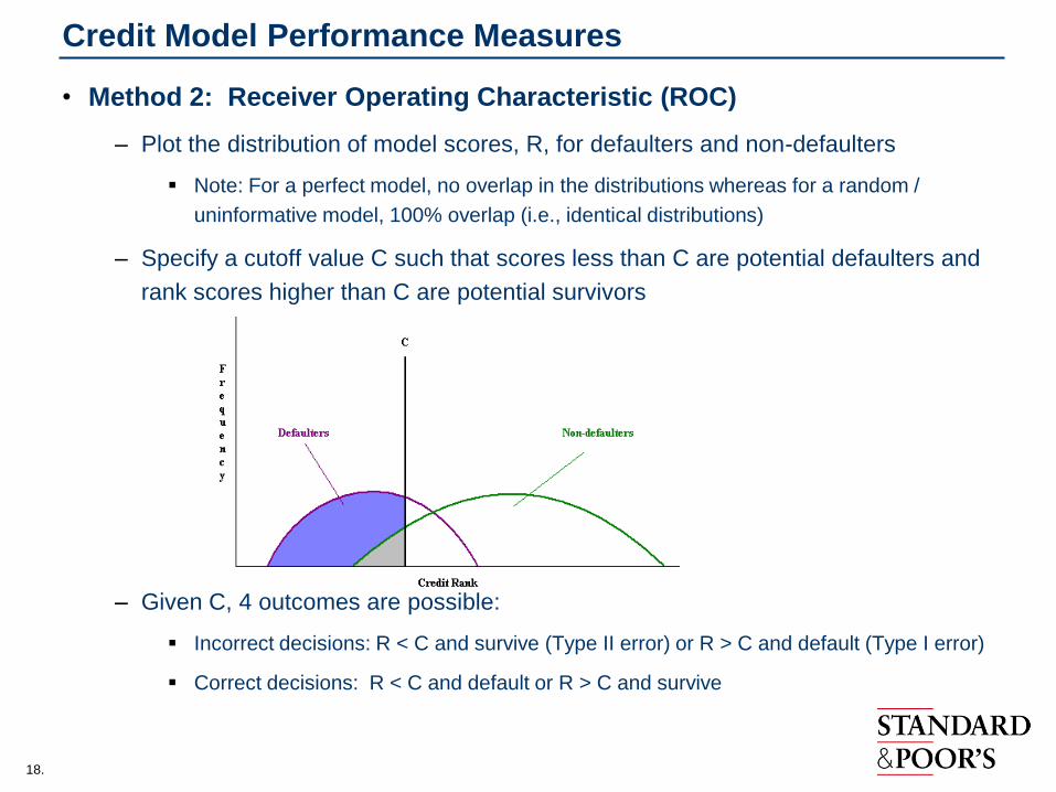
• Method 2: Receiver Operating Characteristic (ROC)
– Plot the distribution of model scores, R, for defaulters and non-defaulters
Note: For a perfect model, no overlap in the distributions whereas for a random /
uninformative model, 100% overlap (i.e., identical distributions)
– Specify a cutoff value C such that scores less than C are potential defaulters and
rank scores higher than C are potential survivors
– Given C, 4 outcomes are possible:
Incorrect decisions: R < C and survive (Type II error) or R > C and default (Type I error)
Correct decisions: R < C and default or R > C and survive

19.
Credit Model Performance Measures
• Method 2: ROC (cont.)
– Define Hit Rate (given C), HC = # of predicted defaulters/total defaulters
– Define False Alarm Rate (given C), FC = # of non-defaulters predicted to default/
total non-defaulters
– Plot HC vs. FC for all values of C to generate the ROC curve
– The larger the ROC (i.e. the area under the ROC curve - shaded region), implying
higher hit rate to false alarm rate, the better the ranking model
Note: Hit rate corresponds to 1 – Type I Error

20.
Credit Model Performance Measures
• Relationship between ROC and CAP
– If the same weight is attributed to Type I vs. Type II errors, it can be shown that
ROC and CAP communicate the same information
AR = 2 x ROC – 1
(Engelmann, Hayden and Tasche, “Testing Rating Accuracy,” Risk, January 2003)
– ROC is however a more general measure as different weights may be given to
Type I and II errors.
Typically, more weight may be given to Type I vs. Type II error
– Example: Giving a loan to a defaulting firm (I) vs. losing potential interest
income by not extending credit to a non-defaulting firm (II)
We assume equivalence of ROC and CAP for this study (i.e. equal weights
to I vs II errors)

21.
Performance Measures: Independent Obligors

22.
Rankings based on PD vs. Default Prediction
• Typical measures: focus on correct identification of defaulters vs. non-
defaulters (binary)
• Credit models: rankings may be based on relative risk (probability or
likelihood)
Implication: A perfect (PD based) ranking model cannot have a perfect
Accuracy Ratio.
– Even the highly ranked “buckets” can have defaults (albeit low)
– The lowest ranked buckets can have survivors (1-PD)
• Example
– Very large pool categorized into 10 equally weighted Risk Category (RC) buckets
on the basis of PD
– Safest bucket (RC1) has PD 2bp, RC2 has PD 4bp, RC3 has PD 8bp, and so on
i.e., each subsequent bucket twice as risky in PD terms
– Large pool (theoretically infinite) ensures realized defaults in each RC bucket
equal expected defaults

23.
Rankings based on PD vs. Default Prediction (Large Pools)
PD (%) % Defaulters % Obligors
RC10 10.24% 50.05% 10.00%
RC9 5.12% 75.07% 20.00%
RC8 2.56% 87.59% 30.00%
RC7 1.28% 93.84% 40.00%
RC6 0.64% 96.97% 50.00%
RC5 0.32% 98.53% 60.00%
RC4 0.16% 99.32% 70.00%
RC3 0.08% 99.71% 80.00%
RC2 0.04% 99.90% 90.00%
RC1 0.02% 100.00% 100.00%
Even with perfect risk categorization on a PD basis, accuracy ratio is only 71.66%.
Default rate matters: If the PDs for all buckets are 5 x larger, CAP curve remains
the same, but the AR = 78.19%.
CAP
0%
20%
40%
60%
80%
100%
0% 10% 20% 30% 40% 50% 60% 70% 80% 90% 100%
% Obligors
% D
efa
ult
ers

24.
Additional Observations for Large Pools
• Even if obligors are categorized on the basis of "noisy" PD estimates,
all results hold provided expected PD for each bucket is monotonic
• Large pools of uncorrelated obligors diversify away "idiosyncratic"
defaults perfectly making realized defaults always equal to expected
defaults
• Buckets defined in terms of PD ranges – both overlapping and non
overlapping will yield similar results
• PDs range can be viewed equivalent to a noisy PD
• Small "noise" component can be made to correspond to distinct PD ranges
• Large "noise" component can be made to correspond to overlapping PD
ranges

25.
Finite Sample Size: Impact of Smaller Pools
• Size of the pool has most impact on AR
values.
• Similar results hold for smaller pools as
large pools with regard to PD
distribution within buckets, both non-
overlapping and overlapping.
26.
Finite Sample Size: Impact of PD levels
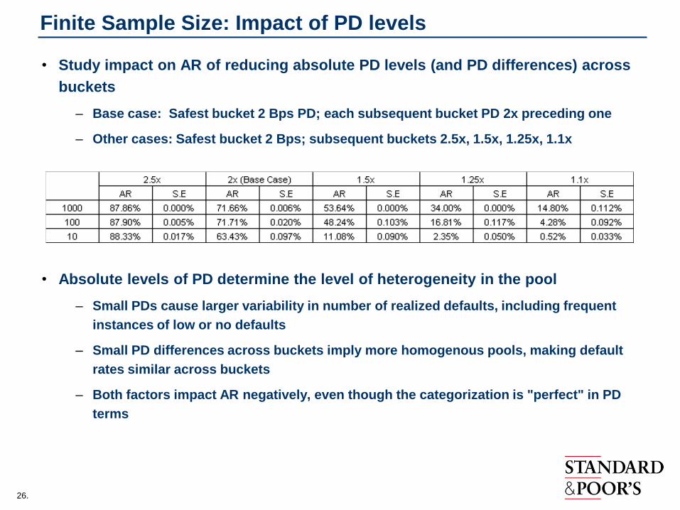
• Study impact on AR of reducing absolute PD levels (and PD differences) across
buckets
– Base case: Safest bucket 2 Bps PD; each subsequent bucket PD 2x preceding one
– Other cases: Safest bucket 2 Bps; subsequent buckets 2.5x, 1.5x, 1.25x, 1.1x
• Absolute levels of PD determine the level of heterogeneity in the pool
– Small PDs cause larger variability in number of realized defaults, including frequent
instances of low or no defaults
– Small PD differences across buckets imply more homogenous pools, making default
rates similar across buckets
– Both factors impact AR negatively, even though the categorization is "perfect" in PD
terms

27.
Performance Measures: Correlated Obligors

28.
Correlation
Fact: - Correlation does not affect a pool‟s expected defaults, …
- … but correlation introduces more variability in realized defaults
Recall: AR being a non-linear function of defaults, i.e., ED(AR) ≠ AR(ED), any
change in shape of the default distribution introduced by correlation
can be expected to impact AR
Correlation modeled in the context of a Systemic Risk factor model
– For a pool of N obligors, most generic model would be to specify a joint
distribution of [u1, u2, …, uN], ui ~ U[0,1] through a copula function and
define obligor i as a default if ui < PDi
– Factor model representation allows for systemic/idiosyncratic separation
Note: Z may be dependent on several independent factors. We assume
a single factor model for the following analysis.
1i i i iZ
29.
Correlation (continued)
• Key feature of model: Conditional independence i.e., conditioned on
systemic latent factors:
• Unconditional PDs for correlated obligors become conditional PDs for
independent obligors
• A given period‟s observation corresponds to a specific systemic latent factor
realization and can be viewed as a description of a given state of the
economy
• Unconditional results can be viewed as an average (over systemic
factors) of conditional, independent results
30.
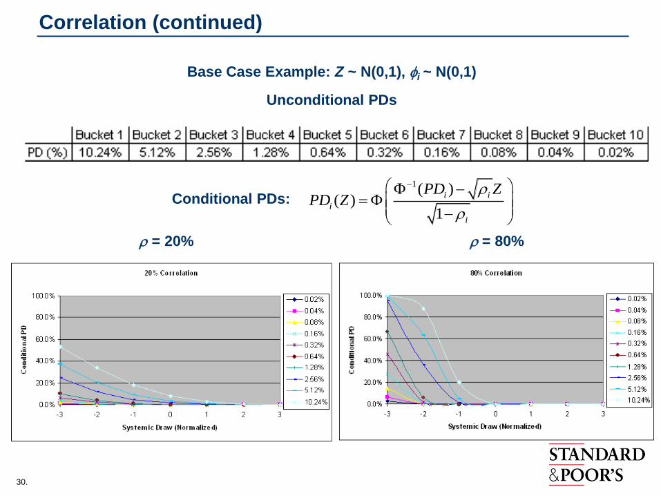
Correlation (continued)
Base Case Example: Z ~ N(0,1), i ~ N(0,1)
Unconditional PDs
Conditional PDs:
= 20% = 80%
1( )( )
1
i i
i
i
PD ZPD Z
31.
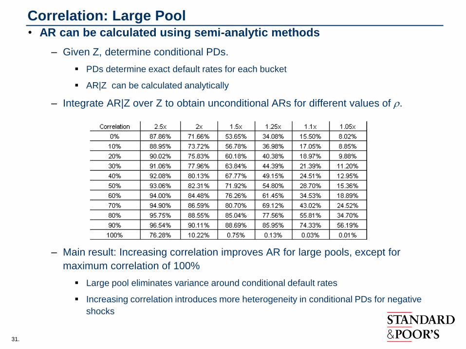
Correlation: Large Pool• AR can be calculated using semi-analytic methods
– Given Z, determine conditional PDs.
PDs determine exact default rates for each bucket
AR|Z can be calculated analytically
– Integrate AR|Z over Z to obtain unconditional ARs for different values of .
– Main result: Increasing correlation improves AR for large pools, except for
maximum correlation of 100%
Large pool eliminates variance around conditional default rates
Increasing correlation introduces more heterogeneity in conditional PDs for negative
shocks
32.
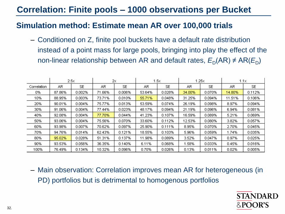
Correlation: Finite pools – 1000 observations per Bucket
Simulation method: Estimate mean AR over 100,000 trials
– Conditioned on Z, finite pool buckets have a default rate distribution
instead of a point mass for large pools, bringing into play the effect of the
non-linear relationship between AR and default rates, ED(AR) ≠ AR(ED)
– Main observation: Correlation improves mean AR for heterogeneous (in
PD) portfolios but is detrimental to homogenous portfolios

33.
Recap
• Typical performance measures such as AR/CAP or ROC may not be very
informative in measuring performance of credit rankings based on
relative risk (probability or likelihood of default)
– Perfect (PD-based) ranking models do not have perfect ARs.
– ARs may vary over time simply due to variations in population default rates
• Typical measures are more meaningful when used for comparing different
categorization models over the same data set
• Correlated changes in credit risk - resulting in very few or large numbers
of obligor defaults - make Typical measures very volatile and difficult to
interpret.
34.
Price and Credit Risk

35.
Price and Credit Risk
• A security‟s price depends on a complex interaction of several risk factors:
– Credit Risk (default, transition, recovery, correlation, exposure size)
– Interest Rate Risk
– Liquidity
– Demand and Supply Conditions
– Other factors such as reinvestment / prepayment risks, etc. depending on the type of security
(MBS for example).
• Rarely is it possible to fully ascertain the contribution of each risk driver to a
security‟s price – even for simple securities
• Arbitrage pricing models make certain assumptions related to price –
Example: CDS spreads reflect default risk
– E [ PV of spread payments ] (fixed leg) = E [ PV of losses ] (floating leg)
– Expected payment values depend on probability of default
– Pricing Theory: Cashflow discounting done using risk-free rate while probabilities of default and
expected recoveries are computed under the „Risk Neutral‟ measure
– Any impact of factors such as liquidity, demand/supply imbalances, systemic risk and market
price of risk, etc. that impact CDS spreads get embedded in the implied risk neutral default
intensities (measure of credit risk)

36.
Price and Credit Risk
• Model interpretations of default risk, perhaps adequate representations of
reality in normal times, may break down in stressed environments.
– CDS spreads for very stable firms impacted in similar ways to more risky firms at the
peak of the crisis
– Across the board re-pricing of all types of structured securities, regardless of the
type of assets backing these securities.
Senior CLO tranches being quoted at spreads wider than the average spread of the
underlying loan portfolio.
37.
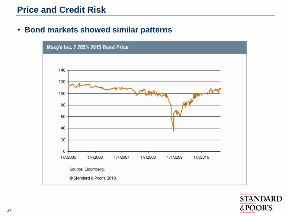
Price and Credit Risk
• Bond markets showed similar patterns

38.
Case Study: Senior CLO Tranche Prices During Credit Crisis
• Some notes:
– Structured securities trades typically executed over the counter that make prices
opaque (i.e. absence of a marketplace that could enable price discovery).
– Inherently complex: Not only require predicting the likely evolution of the underlying
collateral in the future but also accurately modeling the structure waterfall itself.
– More prone to „model risk‟
• Analyze the possible range of default rates, discount premia, market
Sharpe ratio, etc. implied by quoted prices of senior CLO (AAA) tranches
– Several CLO structures were analyzed with senior tranches quoted about 70¢.
– Horizon of 10 years.
– Results are presented here for a specific structure with the lowest break-even
default cushion
– Collateral of CLOs is typically a mix of „BB‟ and „B‟ rated loans
39.
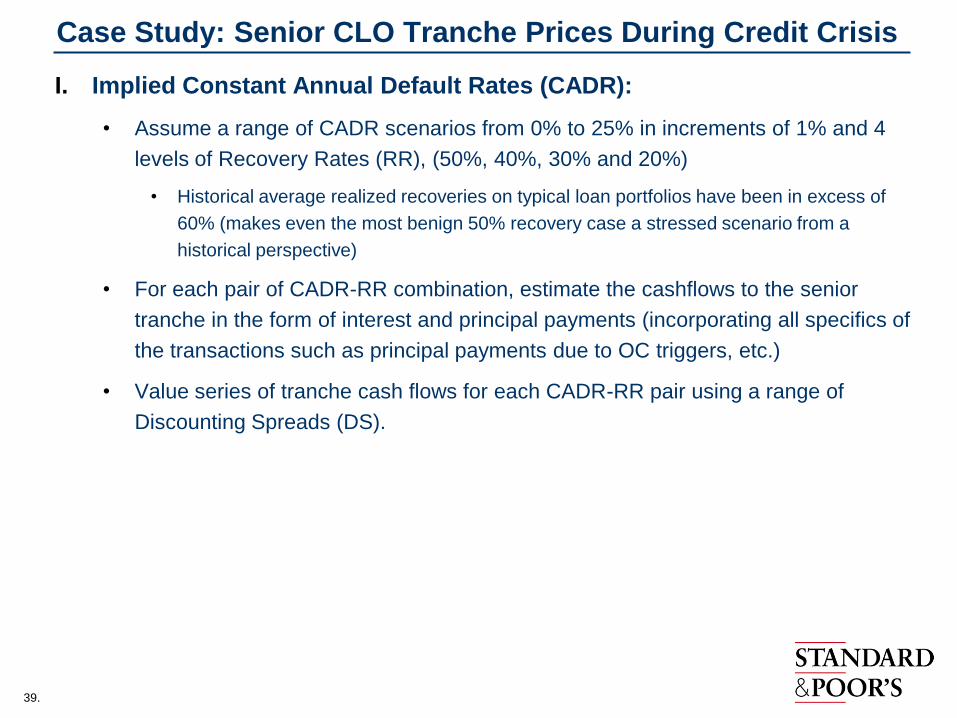
Case Study: Senior CLO Tranche Prices During Credit Crisis
I. Implied Constant Annual Default Rates (CADR):
• Assume a range of CADR scenarios from 0% to 25% in increments of 1% and 4
levels of Recovery Rates (RR), (50%, 40%, 30% and 20%)
• Historical average realized recoveries on typical loan portfolios have been in excess of
60% (makes even the most benign 50% recovery case a stressed scenario from a
historical perspective)
• For each pair of CADR-RR combination, estimate the cashflows to the senior
tranche in the form of interest and principal payments (incorporating all specifics of
the transactions such as principal payments due to OC triggers, etc.)
• Value series of tranche cash flows for each CADR-RR pair using a range of
Discounting Spreads (DS).

40.
Case Study: Senior CLO Tranche Prices During Credit Crisis
• Combination of CADR-RR-DS that produce a discounted cash
flow value of 70¢
41.
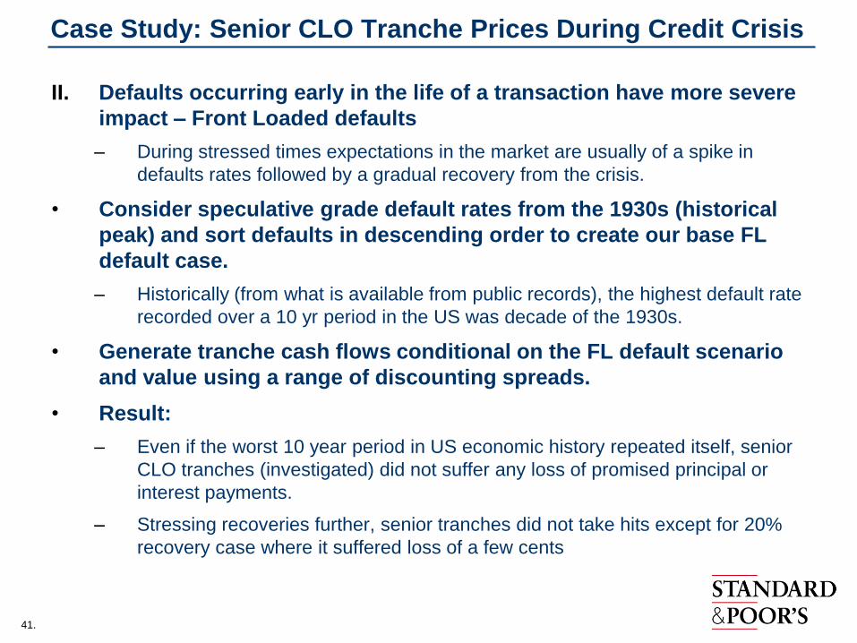
Case Study: Senior CLO Tranche Prices During Credit Crisis
II. Defaults occurring early in the life of a transaction have more severe
impact – Front Loaded defaults
– During stressed times expectations in the market are usually of a spike in
defaults rates followed by a gradual recovery from the crisis.
• Consider speculative grade default rates from the 1930s (historical
peak) and sort defaults in descending order to create our base FL
default case.
– Historically (from what is available from public records), the highest default rate
recorded over a 10 yr period in the US was decade of the 1930s.
• Generate tranche cash flows conditional on the FL default scenario
and value using a range of discounting spreads.
• Result:
– Even if the worst 10 year period in US economic history repeated itself, senior
CLO tranches (investigated) did not suffer any loss of promised principal or
interest payments.
– Stressing recoveries further, senior tranches did not take hits except for 20%
recovery case where it suffered loss of a few cents

42.
Case Study: Senior CLO Tranche Prices During Credit Crisis
• Stress default rates from the Depression era by a factor of 25% and 50%
– Even under these extreme scenarios, only under the 30% and 20% recovery cases did senior
tranches suffer small losses
• Similar results when FL scenario created from 10 highest historical annual
speculative grade default years (sorted in descending order and corresponding
to the years 1933, 1932, 2001, 1991, etc.)

43.
Price Implied Market Sharpe Ratio
• Estimate a market Sharpe ratio (market price of risk) in the context of
the Merton (1974) structural model.
– Structural model provides a framework for pricing securities through a
transformation between physical probabilities of default (PD) and their risk neutral
counterparts
• Approach: Start with assumption that market expectation is a repeat of
the Great Depression era default rates.
• Uncertainty around this expectation modeled in the form of „residual‟
correlation among the underlying loans in the CLO asset pool (pool is
assumed to be 200 homogenous names).
• Numerically solve for L in equation above for values of given base
assumption that Pt corresponds to the 10 year „Great Depression‟
speculative grade default rate witnessed during the 1930‟s.
– L estimation done subject to the constraint that risk neutral default distribution of
collateral portfolio prices the representative senior CLO tranche to about 70¢.
1( )Q
t tP P t L

44.
Price Implied Market Sharpe Ratio
• Market Sharpe ratio corresponding to various correlation assumptions
(5%-20%) estimated in the range of 1.3 to 2.6.
– Historically, L from corporate bond prices estimated in a range of 0.25 to 0.5
[Bohn(2000)]
– Estimates of ex-post Sharpe ratios from equity markets computed around 0.3
[French et al (1987), Fama and French (1989)]
• Market prices of risk/Sharpe ratios could diverge across different asset
classes with capital markets known to be less than perfectly efficient -
however, extent of deviation for CLO tranche price based measure
points to a level of risk aversion not supported by „fundamentals‟.
• Currently senior CLO tranches trade in the low 90s.
Prices reveal useful information related to credit risk;
market inefficiencies/sentiment however cloud the
picture of actual credit risk.

45.
CDS Spread-based Models for Predicting Credit Transitions

46.
CDS Market Derived Signals
• Modeling Objective
– Use CDS spreads to determine a market view of credit quality and
evaluate relative to a fundamental credit analysis benchmark (S&P
Credit Ratings)
• Model: Use CDS data to determine a statistical relationship between
CDS spreads and S&P rating levels
– Adjust for CW/OL, Industry (GICS classification), Region, and
Document Type
• Model Output:
– Representative CDS spreads for each rating level (credit curve)
– The market-implied credit ranking for a firm given its CDS spread and
the value of the other covariates (CW/OL etc)

47.
CDS Market Derived Signals : Model
• Ordinary Least Squares regression to determine the coefficients that
best explain the relationship between observed log-spreads and rating,
firm and contract details.
– Log(Spread) = Piecewise linear function of S&P rating (on a numeric scale)
+ Adjustment for CW/OL status
+ Adjustment for GICS classification
+ Adjustment for Document Type
+ Error term
• Model made more robust through use of Bayesian prior on the model
parameters
– Ensure there is always a solution, even when data is missing for some ratings, GICS, CW/OLs
or DOCs
– Create an appropriate balance between continuity to past data and fidelity to current data
If today‟s data are few, then rely to some degree on previous day‟s results
Let historical relationship between parameters have some influence on how today‟s parameters relate to
each other
• Compute CDS implied rank for a firm by solving for numerical rank that
gives actual spread in above model with zero error.
48.
CDS Market Derived Signals : Discrepancy
• Discrepancy is difference between the computed rank and the actual
S&P rating (Computed Rank – S&P Rating).
• Some of the questions we try to investigate:
– Does a large positive discrepancy suggest that the market is anticipating
an S&P downgrade or rating action?
Similarly, does a large negative discrepancy suggest that the that the market
is anticipating an upgrade?
– Are day-to-day discrepancies as informative as persistent
discrepancies?
– How may large discrepancies be interpreted?
Does the CDS market have a substantially different perspective on the firm‟s
credit risk?
Is the CDS market responding to non-credit aspects regarding the firm
(liquidity, price volatility, and non-credit arbitrage/relative value
opportunities)?
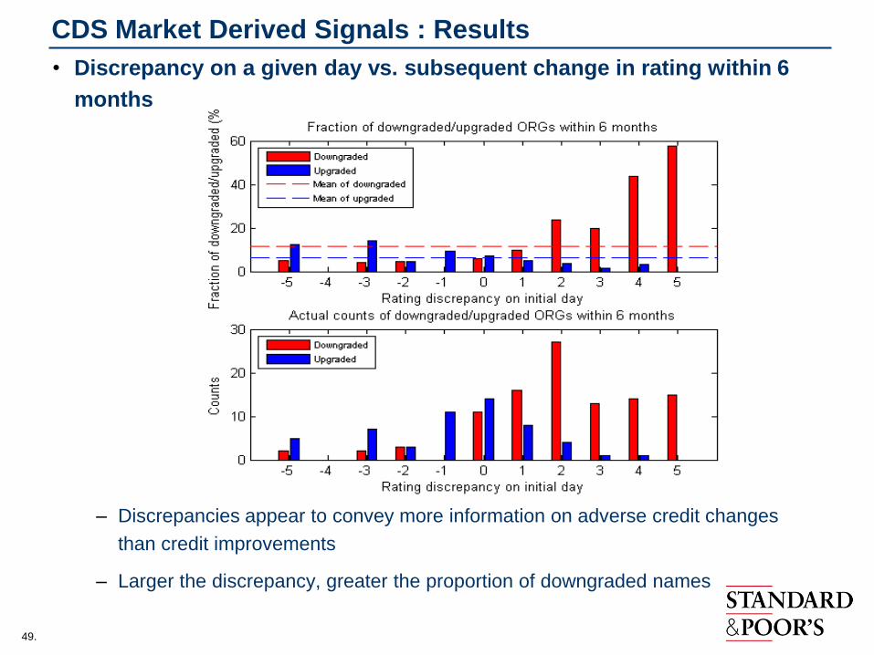
49.
• Discrepancy on a given day vs. subsequent change in rating within 6
months
– Discrepancies appear to convey more information on adverse credit changes
than credit improvements
– Larger the discrepancy, greater the proportion of downgraded names
CDS Market Derived Signals : Results

50.
• Issues with the approach
– Daily discrepancies are volatile
Large discrepancies on a given day very often decline in magnitude before
the actual rating action.
Number of instances where discrepancies are large is small i.e. fraction of
downgraded/upgraded names based on small number of events
• Look at persistent discrepancies to address volatility issues
– Compute a moving average of discrepancy to smooth the deviations
– Define certain criteria for persistence
Average/Min/Max of (MA of) discrepancy exceeds some threshold for a
chosen period length (Signal Persistence Period) before the credit change
– If persistent discrepancy preceded a credit change, consider MDS
information as relevant
CDS Market Derived Signals : Results

51.
CDS Market Derived Signals : Results
• We see instances in the data where CDS MDS seems to provide
informative signals of credit changes
0 100 200 300 400 500 600 700 800 900 10000
2
4
6
8
10
12
Days
Rating
American Express Company
MDS
Rating
0 100 200 300 400 500 600 700 800 900 10002
3
4
5
6
7
8
9
10
Days
Rating
Boeing Co.
MDS
Rating

52.
CDS Market Derived Signals : Results
• But we see (more) instances of false positives i.e. discrepancies
reducing over time and CDS MDS converging to S&P rating

53.
CDS Market Derived Signals : Results
• Also, S&P rating changes are very frequently accompanied by
announcements related to Outlook/Credit Watch
– CDS market expects subsequent rating actions in the future and prices
this expectation
– Future changes in credit driven primarily by CW/OL status
• Controlling for CW/OL, less than 10% of persistent
discrepancies (of 4 notches or more) precede credit changes for
sub-investment grade names.
– Corresponding number for investment grade names is about 6%
• Overall, instances of signals unrelated to credit quality changes
are very high

54.
CDS Market Derived Signals : Results
• Accuracy Ratio for MDS as predictor of credit changes
– Rank order names on the basis of discrepancy and compute AR from
the proportion of names that actually had a credit change
Maximizing AR by „optimizing‟ Average Discrepancy Computation, Signal
Persistence, and Rating Evaluation Periods.
For downgrades, the optimal signal had an AR = 45%.
For upgrades, AR = 30%
ARs for high yield downgrades (50%) and investment grade upgrades (40%)
are higher
ARs may be biased upwards as signals that lead to opposite credit changes
are not penalized
• The caveats discussed earlier about Accuracy Ratio as a
measure of credit model performance apply here also.
55.
References and Credits
• Bohn, J. R., “An Empirical Assessment of a Simple Contingent-
Claims Model for the Valuation of Risky Debt”, The Journal of
Risk Finance, Summer 2000, pp 55-77
• French, K.R., G.W. Schwert, and R.F. Stambaugh. “Expected
Stock Returns and Volatility”, Journal of Financial Economics,
19 (1987), pp. 3-29
• Fama, E.F., and K.R. French. “Business Conditions and
Expected Returns on Stocks and Bonds.” Journal of Financial
Economics, 25 (1989), pp. 23-49.
Many thanks to:
S&P‟s Quantitative Analytics Research Group

56.
www.standardandpoors.com
Copyright © 2011 by Standard & Poor’s Financial Services LLC (S&P), a subsidiary of The McGraw-Hill Companies, Inc. All rights reserved. No content (including ratings, credit-related
analyses and data, model, software or other application or output therefrom) or any part thereof (Content) may be modified, reverse engineered, reproduced or distributed in any form by any
means, or stored in a database or retrieval system, without the prior written permission of S&P. The Content shall not be used for any unlawful or unauthorized purposes. S&P, its affiliates, and
any third-party providers, as well as their directors, officers, shareholders, employees or agents (collectively S&P Parties) do not guarantee the accuracy, completeness, timeliness or availability of
the Content. S&P Parties are not responsible for any errors or omissions, regardless of the cause, for the results obtained from the use of the Content, or for the security or maintenance of any data
input by the user. The Content is provided on an “as is” basis. S&P PARTIES DISCLAIM ANY AND ALL EXPRESS OR IMPLIED WARRANTIES, INCLUDING, BUT NOT LIMITED TO,
ANY WARRANTIES OF MERCHANTABILITY OR FITNESS FOR A PARTICULAR PURPOSE OR USE, FREEDOM FROM BUGS, SOFTWARE ERRORS OR DEFECTS, THAT THE
CONTENT’S FUNCTIONING WILL BE UNINTERRUPTED OR THAT THE CONTENT WILL OPERATE WITH ANY SOFTWARE OR HARDWARE CONFIGURATION. In no event
shall S&P Parties be liable to any party for any direct, indirect, incidental, exemplary, compensatory, punitive, special or consequential damages, costs, expenses, legal fees, or losses (including,
without limitation, lost income or lost profits and opportunity costs) in connection with any use of the Content even if advised of the possibility of such damages.
Credit-related analyses, including ratings, and statements in the Content are statements of opinion as of the date they are expressed and not statements of fact or recommendations to purchase,
hold, or sell any securities or to make any investment decisions. S&P assumes no obligation to update the Content following publication in any form or format. The Content should not be relied on
and is not a substitute for the skill, judgment and experience of the user, its management, employees, advisors and/or clients when making investment and other business decisions. S&P’s opinions
and analyses do not address the suitability of any security. S&P does not act as a fiduciary or an investment advisor. While S&P has obtained information from sources it believes to be reliable,
S&P does not perform an audit and undertakes no duty of due diligence or independent verification of any information it receives.
S&P keeps certain activities of its business units separate from each other in order to preserve the independence and objectivity of their respective activities. As a result, certain business units of
S&P may have information that is not available to other S&P business units. S&P has established policies and procedures to maintain the confidentiality of certain non–public information
received in connection with each analytical process.
S&P may receive compensation for its ratings and certain credit-related analyses, normally from issuers or underwriters of securities or from obligors. S&P reserves the right to disseminate its
opinions and analyses. S&P's public ratings and analyses are made available on its Web sites, www.standardandpoors.com (free of charge), and www.ratingsdirect.com and
www.globalcreditportal.com (subscription), and may be distributed through other means, including via S&P publications and third-party redistributors. Additional information about our ratings
fees is available at www.standardandpoors.com/usratingsfees.
STANDARD & POOR’S and S&P are registered trademarks of Standard & Poor’s Financial Services LLC.