mechanics of earthquakes - semantic scholar...mechanics of earthquakes 209 monotonically increases...

Annu. Rev. Earth Planet. Sci. 1994.22:207-37Copyright © 1994 by Annual Reviews Inc. All rights reserved

MECHANICS OF EARTHQUAKES

H. Kanamori

Seismological Laboratory, California Institute of Technology, Pasadena,California 91125

KEY WORDS: stress drop, static stress drop, dynamic stress drop, kinetic friction

INTRODUCTION

An earthquake is a sudden rupture process in the Earth’s crust or mantlecaused by tectonic stress. To understand the physics of earthquakes it isimportant to determine the state of stress before, during, and after anearthquake. There have been significant advances in seismology duringthe past few decades, and some details on the state of stress near earthquakefault zones are becoming clearer. However, the state of stress is generallyinferred indirectly from seismic waves which have propagated throughcomplex structures. The stress parameters thus determined depend on thespecific seismological data, methods, and assumptions used in the analysis,and must be interpreted carefully.

This paper reviews recent seismological data pertinent to this subject,and presents simple mechanical models for shallow earthquakes. Scholz(1989), Brune ( 1991 ), Gibowicz (1986), and Udias (1991 ) recently this subject from a different perspective, and we will try to avoid dupli-cation with these papers as much as possible. Because of the limited space,available, this review is not intended to be an exhaustive summary of theliterature, but reflects the author’s own view on the subject.

Throughout this paper we use the following notation unless indicatedotherwise: e= P-wave velocity, /~= S-wave velocity, Vr=rupturevelocity, ~ = fault particle-motion velocity, ¢r0 = tectonic shear stress onthe fault plane before an earthquake, a ~ = tectonic shear stress on the faultplane after an earthquake, A~r = a0-~r~ = static stress drop, af = kineticfrictional stress during faulting, A(ra = ~o-6f = dynamic (kinetic) stressdrop, 5’ = fault area, D = fault offset,/} = 2t) = fault offset particle vel-

2070084-6597/94/0515-0207505.00

www.annualreviews.org/aronlineAnnual Reviews

Ann

u. R

ev. E

arth

Pla

net.

Sci.

1994

.22:

207-

237.

Dow

nloa

ded

from

arj

ourn

als.

annu

alre

view

s.or

gby

Cal

ifor

nia

Inst

itute

of

Tec

hnol

ogy

on 0

8/10

/07.

For

per

sona

l use

onl

y.

http://www.annualreviews.org/aronline

208 KANAMORI

0city, M-- earthquakemoment.

magnitude, #=rigidity, Mo = #DS = seismic

TECTONIC STRESS

The rupture zones of earthquakes are usually planar (fault plane), butoccasionally exhibit a complex geometry. The stress distribution near afault zone varies as a function of time and space in a complex manner.Before and after an earthquake (interseismic period), the stress variesgradually over a time scale of decades and centuries, and during an earth-quake (coseismic period) it varies on a time scale of a few seconds to a fewminutes.

The stress variation during an interseismic period can be consideredquasi-static. It varies spatially with stress concentration near locationswith complex fault geometry. We often simplify the situation by con-sidering static stress averaged over a scale length of kilometers. We callthis stress field the "macroscopic static stress field." In contrast, we callthe stress field with a scale length of local fault complexity the "microscopicstatic stress field."

During an earthquake, stress changes very rapidly. It decreases in mostplaces on the fault plane, but it may increase at some places, especiallynear the edge of a fault where stress concentration occurs. We call thestress field averaged over a time scale of faulting the "macroscopic dynamicstress field," and that with a time scale of rupture initiation, the "micro-scopic dynamic stress field."

Macroscopic Static Stress Field

Figure 1 shows a schematic time history of macroscopic static stress overthree earthquake cycles. After an earthquake the shear stress on the fault

b.Stress

o0

Ao= Oo_O1_ 30t0100bars °t

TimeTR-300 years

Stress

Time

Figure 1 Schematic figure showing temporal variations of macroscopic (quasi-)static stresson a fault plane. (a) Weak fault model. (b) Strong fault model.


Ann

u. R

ev. E

arth

Pla

net.

Sci.

1994

.22:

207-

237.

Dow

nloa

ded

from

arj

ourn

als.

annu

alre

view

s.or

gby

Cal

ifor

nia

Inst

itute

of

Tec

hnol

ogy

on 0

8/10

/07.

For

per

sona

l use

onl

y.


MECHANICS OF EARTHQUAKES 209

monotonically increases from a i to o’0 during an interseismic period. Whenit approaches a0, the fault fails causing an earthquake, and the stress dropsto al, and a new cycle begins. The stress difference A~r = a0- trl is thestatic stress drop, and TR is the repeat time. For a typical sequence alongactive plate boundaries, Aa ~ 30 to 100 bars, and TR ~ 300 years. (Thenumerical values given in the text are representative values for illustrationpurposes only; more details will be given in the section for each parameter.)

The absolute value of a0 and trl cannot be determined directly withseismological methods; only the difference, Atr = cr0-~rl, can be deter-mined. If fault motion occurs againist kinetic (dynamic) friction, trf,repeated occurrence of earthquakes should result in a local heat flowanomaly along the fault zone. From the lack of a local heat flow anomalyalong the San Andreas fault, a relatively low value, 200 bars or less, hasbeen suggested for o-r (Brune et al 1969; Henyey & Wasserburg 1971;Lachenbruch & Sass 1973, 1980). More recent studies on the stress on theSan Andrcas fault zone also suggest a low stress--less than a few hundredbars (Mount & Suppe 1987, Zoback et al 1987). However, the strength rocks (frictional strength) measured in the laboratory suggests that shearstress on faults is high, probably higher than 1 kbar (Byerlee 1970, Brace& Byerlee 1966). Figures la and lb show the two end-member models,the weak fault model (tr 0 ,,~ 200 bars), and the strong fault model (tr0 ~ kbars). In these simple models "strength of fault" refers to ~r0. Actually,~0 and ~1 may vary significantly from place to place and from event toevent; the loading rate may also change as a function of time so that thetime history is not expected to be as regular as indicated in Figure 1.

Microscopic Static Stress Field

An earthquake fault is often modeled with a crack in an elastic medium.Figure 2 shows the distribution of shear stress near a crack tip (e.g. Knopoff

-a I +a -a 0

Initial!stress

+~

Figure 2 Static stress field near a crack tip. (Left) Geometry. A 2-dimensional crack witha width of 2a extending from z = - oo to + oe is formed under shear stress a=.,. = tr 0. (Right)Shear stress azy before (dashed line) and after (solid curves) crack formation.


Ann

u. R

ev. E

arth

Pla

net.

Sci.

1994

.22:

207-

237.

Dow

nloa

ded

from

arj

ourn

als.

annu

alre

view

s.or

gby

Cal

ifor

nia

Inst

itute

of

Tec

hnol

ogy

on 0

8/10

/07.

For

per

sona

l use

onl

y.


210 KANAMORI

1958). For an infinitely thin crack in a purely elastic medium, the stress(azy in Figure 2) is unbounded at the crack tip, and decreases as 1/,v/r the distance r from the crack tip increases (i.e. inverse square-root singu-larity). In a real medium, the material near the crack tip yields at a certainstress level (yield stress) causing the stress near the crack tip to be finite.Nevertheless, the behavior shown in Figure 2 is considered to be a goodqualitative representation of static stress field near a fault tip.

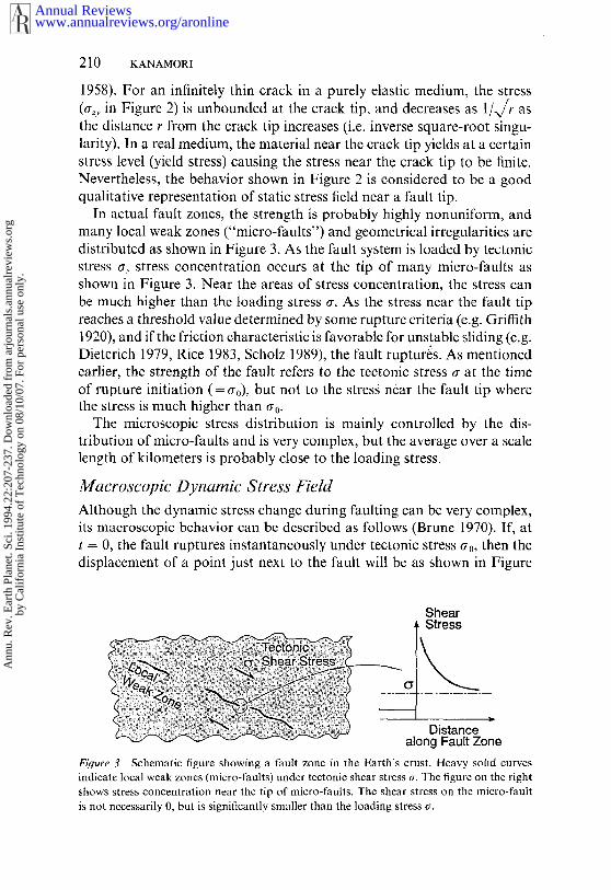
In actual fault zones, the strength is probably highly nonuniform, andmany local weak zones ("micro-faults") and geometrical irregularities aredistributed as shown in Figure 3. As the fault system is loaded by tectonicstress a, stress concentration occurs at the tip of many micro-faults asshown in Figure 3. Near the areas of stress concentration, the stress canbe much higher than the loading stress a. As the stress near the fault tipreaches a threshold value determined by some rupture criteria (e.g. Griffith1920), and if the friction characteristic is favorable for unstable sliding (e.g.Dieterich 1979, Rice 1983, Scholz 1989), the fault ruptures. As mentionedearlier, the strength of the fault refers to the tectonic stress o- at the timeof rupture initiation (= a0), but not to the stresg near the fault tip wherethe stress is much higher than

The microscopic stress distribution is mainly controlled by the dis-tribution of micro-faults and is very complex, but the average over a scalelength of kilometers is probably close to the loading stress.

Macroscopic Dynarnic Stress Field

Although the dynamic stress change during faulting can be very complex,its macroscopic behavior can be described as follows (Brune 1970). If, t = 0, the fault ruptures instantaneously under tectonic stress a0, then thedisplacement of a point just next to the fault will be as shown in Figure

Shear

[Stress

Distancealong Fault Zone

Figure 3 Schematic figure showing a fault zone in the Earth’s crust. Heavy solid cnrvesindicate local weak zones (micro-faults) under tectonic shear stress a. The figure on the rightshows stress concentration near the tip of micro-faults. The shear stress on the micro-faultis not necessarily 0, but is significantly smaller than the loading stress or.


Ann

u. R

ev. E

arth

Pla

net.

Sci.

1994

.22:

207-

237.

Dow

nloa

ded

from

arj

ourn

als.

annu

alre

view

s.or

gby

Cal

ifor

nia

Inst

itute

of

Tec

hnol

ogy

on 0

8/10

/07.

For

per

sona

l use

onl

y.



4a. Fault motion is resisted by kinetic friction af during slippage so thatthe difference Aad = a0-- ar is the effective stress that drives fault motion,and is called the dynamic stress drop. In general Aaa varies with time.Following Brune (1970), Aaa can be related to the particle velocity of one side of the fault. After rupture initiation, the shear disturbancepropagates in the direction perpendicular to the fault (Figure 4a). At timet it reaches the distance fit, beyond which the disturbance has not arrived.Denoting the displacement on the fault at this time by u(t), the instan-taneous strain is u(t)/flt. Since this is caused by Acta,

from which we obtain

u(t) = Aadflt/l~ and fi(t) = (Aaa/#)fl = /) = constant. (1)

Curve (1) in Figure 4b shows u(t) for this case.As the fault rupture encounters some obstacle or the end of the fault,

the fault motion slows down and eventually stops as shown by curve (2)in Figure 4b. This result is in good agreement with the numerical result byBurridge (1969).

Since the fault rupture is not instantaneous, but propagates with a finiterupture velocity Vr, which is usually about 70 to 80% of fl, the actualmacroscopic particle motion is slower than that given by (1). Also, thebeginning of rupture can no longer be given by a linear function of time(e.g. Ida & Aki 1972). Nevertheless, the macroscopic behavior can described by (1) with deceleration of about a factor of 2, as shown

u

Crustal Block~ on One Side of a Fault

.(1)u (t)u .,’" ""

Time

Figure 4 (a) Displacement at time t as a function of fault-normal distance from thefault. The stress on the fault is the cffective stress (dynamic stress drop) Actd - a0-ar. Thedisturbance has propagated to a distance of fit. (b) Particle motion of one side of the faultas a function of time. Curve (1) is for an infinitely long fault when the Aad is appliedinstantaneously. Curve (2) is for a finite fault. Curve (3) is for a finite fault when Aaa applied as a propagating stress.


Ann

u. R

ev. E

arth

Pla

net.

Sci.

1994

.22:

207-

237.

Dow

nloa

ded

from

arj

ourn

als.

annu

alre

view

s.or

gby

Cal

ifor

nia

Inst

itute

of

Tec

hnol

ogy

on 0

8/10

/07.

For

per

sona

l use

onl

y.


212 KANAMORI

curve (3) in Figure 4b. Numerical results by Hanson et al (1971), Mada-riaga (1976), and Richards (1976) support this conclusion. If we denotethe offset and duration of slip by D (=2U) and Tr, then the averagemacroscopic particle velocity is (~)= D/(2Tr). Thus, Equation (1)suggests

(~r) = l(Aad~/3 and AOd -= C 1 (~) (~],/), (2)CI\ [~ ] ’

where c~ is a constant which is of the order of 2.

Microscopic Dynamic Stress Field

Since the theory of cracks in an elastic medium is well established, it ismost convenient to use the results from crack theory to understand thedynamic stress field during faulting. In a real fault zone, the fault geometryis complex, and the strength and material properties are heterogeneous sothat the stress field is very different from that computed for a simplecrack. Nevertheless, the results for a simple crack provide a useful insightregarding the general property of stress and particle motion during fault-ing. Many theoretical studies have been made on this subject (Kostrov1966, Burridge 1969, Takeuchi & Kikuchi 1971, Kikuchi & Takeuchi 1971,Ida 1972, Richards 1976, Madariaga 1976). Here we briefly describe theresults for steady-state crack propagation described by Freund (1979). Thegeometry of the crack is shown in Figure 5a. (This is called the antiplaneshear mode III problem.) The crack expands in the +x direction underuniform far-field stress ayz = a0. The crack propagates at a constant vel-ocity Vr </~ (steady propagation). The crack surface extends from -a a over which the stress is equal to the kinetic friction at. Then Equations(21) and (22) of Freund (1979)

b.

-a - +a ’ X

Figure 5 Steady crack propagation. (a) Geometry (same as Figure 2a). A crack propagatingin the x direction at a velocity of V,.’ (b) The shear stress a,e and particle velocity ~= as function of distance.


Ann

u. R

ev. E

arth

Pla

net.

Sci.

1994

.22:

207-

237.

Dow

nloa

ded

from

arj

ourn

als.

annu

alre

view

s.or

gby

Cal

ifor

nia

Inst

itute

of

Tec

hnol

ogy

on 0

8/10

/07.

For

per

sona

l use

onl

y.



(./x+-a_l)+~o for x>a

fi~=O, a~=(a0--ar)(~-l)+ao for x< -a.

From the condition that there be no stress singularity at the trailing edge

(~0-~0 = ~ ~- , (4~

where U is the total displacement of one side of the crack. The stressdifference e~-~f is the dynamic stress drop ~a defined earlier.

These results are graphically shown in Freund (l 979) and are reproducedin Figure 5b. The typical inverse square-root singularity (1/~ ~ a) is seenfor ~ ahead of the leading edge, and for ~ just behind it.

The degree of singularity depends on the physical condition near thecrack tip, e.g. the dependence of the cohesive force on velocity and dis-placement. In a real fault zone, because of the finite strength of the material,the velocity and stress must be finite.

In principle, we should be able to determine the time history of particlevelocity from seismological observations and compare it to Equation (3),but in practice it is di~cult to determine this uniquely. Seismologically,one observes convolmion of the local slip function shown in Figure 4b andthe rupture propagation effect, and it is di~cult to separate these twofactors. Most commonly, seismologists can determine only the average~article velocity. Using (3) we obtain the average ~arficle velocity

<0> = ~& : ~(~0-~0,

from which

(~o-~) = A~a = ~<O> ~ <0>, (s)

where < = 0.Tfl is assumed. Equation (5) agrees with Equation (2) exceptfor the factor c~, which is of the order of 2. Considering all the uncertaintiesin the determination of <0> and the model, this much of uncertainty is


Ann

u. R

ev. E

arth

Pla

net.

Sci.

1994

.22:

207-

237.

Dow

nloa

ded

from

arj

ourn

als.

annu

alre

view

s.or

gby

Cal

ifor

nia

Inst

itute

of

Tec

hnol

ogy

on 0

8/10

/07.

For

per

sona

l use

onl

y.


214 KANAMORI

inevitable. For simplicity’s sake we will use Equation (5) in the followingdiscussion, but this uncertainty (a factor of 2) must be borne in mind interpreting the particle velocity in terms of Atrd. Husseini (1977) obtaineda similar expression.

The large particle velocity near the leading edge contributes to excitationof high-frequency accelerations, but the actual mechanism is complex. Forcxample, Yamashita (1983) explained the observed accelerations in termsof abrupt changes in rupture propagation, but exactly how high-frequencyaccelerations are excited is still an unresolved problem. High-frequencyaccelerations can be excited by irregular rupture velocity, sudden changesin material strength or sudden changes in frictional characteristics (Aki1979). Chert et al (1987) showed that heterogeneities of both stress dropand cohesion are the main factors that control the growth, cessation, andhealing of the crack, and that the complexities in seismic radiation arecaused by the complex healing process as well as complex rupturepropagation.

In the discussion above, Vr is assumed constant. In a more realisticcase of spontaneous crack propagation, however, Vr is determined by theproperty of the material (cohesive energy, surface energy) and the geometryof the crack, and the degree of stress concentration near the crack tipchanges drastically (Kostrov 1966, Kikuchi & Takeuchi 1971, Burridge1969, Richards 1976). However, in most seismological applications,Vr/[3 ,’~ 0.7 to 0.8 and the model of steady subsonic crack propagation isconsidered reasonable.

SEISMOLOGICAL OBSERVATIONS

Static Stress Drop

Static stress drop Aa can be determined by the ratio of displacement u toan appropriate scale length /~ of the area over which the displacementoccurred:

&r = Cl~(U/E). (6)

This scale length could be the fault length L, the fault width W, or thesquare root of fault area S, depending on the fault geometry.

Since the stress and strength distributions near a fault are nonuniform,the slip and stress drop are in general a complex function of space. In mostapplications, we use the stress drop averaged over a certain area, e.g. theentire fault plane. Locally, the stress drop can be much higher than theaverage (Madariaga 1979). To be exact, the average stress drop is thespatial average of the stress drop. However, the limited resolution ofseismological methods often allows determinations of only the average


Ann

u. R

ev. E

arth

Pla

net.

Sci.

1994

.22:

207-

237.

Dow

nloa

ded

from

arj

ourn

als.

annu

alre

view

s.or

gby

Cal

ifor

nia

Inst

itute

of

Tec

hnol

ogy

on 0

8/10

/07.

For

per

sona

l use

onl

y.



displacement over the fault plane, which in turn is used to compute theaverage stress drop.

Stress drops have been estimated using the following methods:

1. From D and/~ estimated from geodetic data.2. From D estimated from surface break, and S estimated from the

aftershock area.3. From seismic moment M0, and S estimated from either the aftershock

area, surface break, or geodetic data.4. From M0, and /S, estimated from the source pulse width z, or the

characteristic frequency (often called the corner frequency) f0 of thesource spectrum.

5. From the slip distribution on the fault plane determined from high-resolution seismic data.

6. From a combination of the above.

Method 1 was used by Tsuboi (1933) for the 1927 Tango, Japan, earth-quake. Tsuboi concluded that the strain associated with the earthquake isof the order of 10.4 which translatcs to Aa of 30 bars (/~ = 3x 10~dyne/cm2 is assumed). Chinnery (1964) also used this method to concludethat the stress drops of earthquakes are about 10 to 100 bars.

Method 2 is used when geodetic data are not available. Unfortunatelythe surface break does not necessarily represent the slip at depth (someearthquakes do not produce a surface break, e.g. the 1989 Loma Prieta,California, earthquake). In general, the overall extent of the aftershockarea can be taken as the extent of the rupture zone. Although this interpret-ation is not correct in detail (for many earthquakes, the aftershocks donot occur in the area of large slip, but in the surrounding areas), the overalldistribution of the aftershocks appears to coincide with the extent of therupture zone. However, the aftershock area usually expands as a functionof time, and there is always some ambiguity regarding identification ofaftershocks and the aftershock area. Most frequently, the aftershock areadefined at about one day after the main shock is used for this purpose(Mogi 1968), but this definition is somewhat arbitrary.

Method 3 is most commonly used for large earthquakes. The seismicmoment M0 can be reliably determined from long-period surface wavesand body waves for most large earthquakes in the world using the datafrom seismic stations distributed worldwide. When the fault geometry isfixed, the seismic moment is a scalar quantity given by M0 = I~DS. FromM0 and S, D can be determined. If we define the scale length of the faultby/S = S~/z, the avcragc strain changc is e = ell)IS 1/2 where cl is a constantdetermined by the geometry of the fault, and is usually of the order of 1.Then the stress drop is


Ann

u. R

ev. E

arth

Pla

net.

Sci.

1994

.22:

207-

237.

Dow

nloa

ded

from

arj

ourn

als.

annu

alre

view

s.or

gby

Cal

ifor

nia

Inst

itute

of

Tec

hnol

ogy

on 0

8/10

/07.

For

per

sona

l use

onl

y.


216 KANAMORI

Aa = #e = c~,uD/SI/2 (7)

Method 4 is frequently used for relatively small (M < 5) earthquakes.For these events, the seismic moment can be usually determined from bodywaves. For these small earthquakes, the shape of the fault plane is notknown so that a simple circular fault model with radius r is often used. Ifthe source is simple, the pulse width z is approximately equal to r/Vr. Since

Vr ~ 0.7fl, r = c~r/fl, where c2 is a constant of the order of l (Geller 1976,Cohn et al 1982). Another way of determining the source dimension is touse the frequency spectrum of seismic waves. Brune (1970) related thecorner frequency f0 of the S wave spectrum to r. Theoretically, if thesource is simple, the pulse width ~ can be translated to a corner frequencyf0, but if the source is complex, the interpretation off0 is not straight-forward. Because of its simplicity, this method is widely used. However,many assumptions were built into this method (e.g. circular fault etc),so that the values determined for individual events are subject to largeuncertainties, but the average of many determinations is consideredsignificant.

Method 5 is most straightforward in concept, but is difficult to use unlesshigh-quality data are available, preferably in both near- and far-field. Withthe increased availability of strong-motion records, this method is nowwidely used (e.g. Hartzell & Helmberger 1982). The slip function on thefault plane is determined directly, which can be used to estimate not onlythe average stress drop but also local stress drop.

Many determinations of stress drops have been made by combiningthese methods. Figure 6a shows the relation between M0 and S for largeand great earthquakes (Kanamori & Anderson 1975). In general, log is proportional to (2/3) log M0. Since M0 gSD = c/ ~S 3]2, Figure 6aindicates that Aa is constant over a large range of M0. The straight linesin Figure 6a show the trends for circular fault models with Aa = 1, 10,and 100 bars. The actual value of the stress drop depends on the faultgeometry and other details, but the overall trend appears well established.Stress drop Aa varies from 10 to 100 bars for large and great earthquakes.

For smaller earthquakes, it is necessary to use higher frequency wavesto determine source dimensions, but the strong attenuation and scatteringof high-frequency waves make the determination of source dimensionsmore difficult. Because of this difficulty, whether the trend shown in Figure6a continues to very small source dimensions or not has been debated.Several studies indicate that it breaks down at r = 100 m, but a recentresult obtained by Abercrombie & Leary (1993) from down-hole (2.5 kin)observations near Cajon Pass, California, suggests that the trend continuesto at least r = 10 m, as shown in Figure 6b.


Ann

u. R

ev. E

arth

Pla

net.

Sci.

1994

.22:

207-

237.

Dow

nloa

ded

from

arj

ourn

als.

annu

alre

view

s.or

gby

Cal

ifor

nia

Inst

itute

of

Tec

hnol

ogy

on 0

8/10

/07.

For

per

sona

l use

onl

y.


MECHANICSOFEARTHQUAKES 217

ao

106 ’ I ’ I ’ I ’ I¯ Inter-Ploleo Inlro-Plate ~o~"Ios ¢~.~ ~

104

2~

(S in km2)

10110~ I ~ I = I = I

1027 i028 1029 1050

Mo, dyne-era

bo

101° Lines of constant stress drop(bars)

U~ 104

~ ~ ~ ~ ......"~ 10~ 10~ 10t~ 10~ 10ts 10~ 10~ 10~

Seismic Moment (Nm)

Figure ~ (a) ~clation between fault area S alld seismic moment Mo, for large and greatearthquakes (Kanamori & Anderson 19~5). (b) Relation between seismic moment M0 andsource area for small and large earthquak~ (Abercrombie & Leafy 1993),


Ann

u. R

ev. E

arth

Pla

net.

Sci.

1994

.22:

207-

237.

Dow

nloa

ded

from

arj

ourn

als.

annu

alre

view

s.or

gby

Cal

ifor

nia

Inst

itute

of

Tec

hnol

ogy

on 0

8/10

/07.

For

per

sona

l use

onl

y.


218 KANAMORI

These results suggest that Ae averaged over a distance of 100 m orlonger appears to be within a range of 1 to 1000 bars, for a range of M0from 1016 to 1030 dyne-cm. The implications of the constant stress drophave been discussed by many investigators (e.g. Aki 1971, Hanks 1979).

Hiyh Stress-Drop Events

As shown in Figures 6a and 6b, the static stress drops of most large(M > 5.5 or Mo > 2.2 × 1024 dyne-cm) earthquakes are in the range of 10to 100 bars, but there are some exceptions. Moderate earthquakes withvery high stress drops (300 bars to 2 kbars) are occasionally observed. Forexample, Munguia & Brune (1984) found very high stress-drop (up to kbars) earthquakes in the area of the 1978 Victoria, Baja California,earthquake swarm. These earthquakes are characterized by high-frequencysource spectra. To identify these high stress-drop earthquakes, near-fieldobservations are necessary. As the distance increases, the attenuationof high-frequency energy makes it difficult to identify high stress-dropearthquakes.

Recently several high stress-drop earthquakes were observed with close-in wide-dynamic range seismographs. For example, Kanamori et al (1990,1993) estimated Aa of the 1988 Pasadena, California, earthquake(M = 4.9) to be 300 bars to 2 kbars over a source dimension of about 0.5kin. Another example is the 1991 Sierra Madre, California, earthquake(M = 5.8). Wald (1992) and Kanamori et al (1993) estimated Aa to to 300 bars over a source dimension of about 4 km. The large range givento these estimates is due to the uncertainty in the source dimension andrupture geometry. Nevertheless, there is little doubt that these earthquakeshave a significantly larger stress drop than most earthquakes. These resultsindicate that Ae can be very large over a scale length of a few kin. In mostlarge earthquakes, regions of high and low stress drops are averaged outresulting in Ae of 10 to 100 bars.

Although these high stress-drop earthquakes may occur only in specialtectonic environments, we consider that they represent an end-member ofearthquake fault models, as we discuss later.

Dynamic Stress Drop

As discussed earlier, the dynamic stress drop Aad is the stress that drivesfault motion, and controls the particle velocity of fault motion. The particlevelocity ~ of fault motion is thus an important seismic source parameterthat provides estimates of Aad, through relations like (2) or (5).

Maximum ground motion velocities recorded by strong motion instru-ments provide crude estimates of the particle velocity of fault motion.Brune (1970) suggested, using the data from six earthquakes, an upper


Ann

u. R

ev. E

arth

Pla

net.

Sci.

1994

.22:

207-

237.

Dow

nloa

ded

from

arj

ourn

als.

annu

alre

view

s.or

gby

Cal

ifor

nia

Inst

itute

of

Tec

hnol

ogy

on 0

8/10

/07.

For

per

sona

l use

onl

y.



limit of the particle velocity of 1 m/sec. A compilation of strong-motiondata by Heaton et al (1986, figure 20) also indicates that the upper limitof the observed ground motion velocity is about 1 m/sec.

Unfortunately, direct determination of ~ is not very easy because theobserved waveform is the convolution of the local dislocation functionand the fault rupture function. Kanamori (1972) estimated ~2 for the 1943Tottori, Japan, earthquake to be about 42 cm/sec using a very simple faultmodel. A similar method was used to determine the particle velocities forseveral Japanese earthquakes: 1 m/sec for the 1948 Fukui earthquake(Kanamori 1973), 50 cm/sec for the 1931 Saitama earthquake (Abe 1974a),30 cm/sec for the 1963 Wakasa Bay earthquake (Abe 1974b), and cm/sec for the 1968 Saitama earthquake (Abe 1975). These results indicatea range of Aad from 40 to 200 bars (using 2) and 20 to 100 bars (using Boatwright (1980) developed a method to determine dynamic stress dropsfrom seismic body waves.

Some eyewitness reports suggest somewhat larger particle velocities, buteven if we allow for the uncertainties in the measurements, ~ appears tobe bounded at about 2 m/sec.

For more recent earthquakes, the distribution of slip and particle vel-ocity is determined by seismic inversion. Heaton (1990) estimated Aad forseveral earthquakes from the particle motion velocities thus determined.His estimate ranges from 12 to 40 bars for the average Aad, and from 22to 84 bars for the local Aad.

Quin (1990) and Miyatake (1992a,b) attempted to determine Aad the slip time history estimated by seismic inversion. Quin (1990) modeledthe dynamic stress release pattern of the 1979 Imperial Valley, California,earthquake using the slip distribution determined by Archuleta (1984).Miyatake (1992a,b) used the slip models for the Imperial Valley earthquakeand several Japanese earthquakes determined by Takeo (1988) and Takeo& Mikami (1987), and estimated the static stress drop Aa on the faultplane from the slip distribution. Assuming that Aad = Aa, he computedthe local slip function using the method developed by Mikumo et al (1987).A good agreement between the computed slip function and that determinedby seismic inversion led him to conclude that Aad ~ A~r (within a factorof 2), which is in good agreement with Quin’s (1990) result. Since the risetime of local slip function determined by seismic inversion is usuallyconsidered to be the upper limit (a very short rise time cannot be resolvedwith the available seismic data), the conclusion by Quin and Miyatakeindicates that z~aa is comparable to A~r, or possibly larger. However, Aadis unlikely to be much higher than 200 bars, because the observed particlevelocity seems to be bounded at about 2 m/see.

McGuire & Hanks (1980) and Hanks & McGuire (1981) related


Ann

u. R

ev. E

arth

Pla

net.

Sci.

1994

.22:

207-

237.

Dow

nloa

ded

from

arj

ourn

als.

annu

alre

view

s.or

gby

Cal

ifor

nia

Inst

itute

of

Tec

hnol

ogy

on 0

8/10

/07.

For

per

sona

l use

onl

y.


220 KANAMORI

root-mean-square (RMS) acceleration to stress drop. Using this relation,Hanks & McGuire (1981) estimated stress drops for many Californiaearthquakes to be about 100 bars. This estimate, obtained from the radi-ated wave field rather than the static field, can be regarded as a measureof the average A~a.

In summary, Aa~ varies over a range of 20 to 200 bars, which is approxi-mately the same as that for A~.

Asperities and Barriers

Many studies have shown that slip distribution on a fault is very complex,i.e. most large earthquakes are multiple events at least on a time scale ofa few seconds to a few minutes (e.g. Imamura 1937, Miyamura et al 1964,Wyss & Brune 1967, Kanamori & Stewart 1978). Recent seismic inversionstudies have shown this complexity in great detail for earthquakes in bothsubduction zones (e.g. Ruff & Kanamori 1983; Lay et al 1982; Beck Ruff 1987, 1989; Schwartz & Ruff 1987; Kikuchi & Fukao 1987) and incontinental crusts (see Heaton 1990 for a summary). Two examples areshown in Figure 7 (Wald et al 1993, Mendoza & Hartzell 1989).

These models have been often interpreted in terms of barriers--areaswhere no slip occurs during a main shock (Das & Aki 1977), and asperi-ties-areas where large slip occurs during a main shock (e.g. Kanamori1981). The mechanical properties of the areas between asperities are poorlyunderstood. One possibility is that the slip there occurs gradually in theform of creep and small earthquakes during the interseismic periods. If thisis the case, the same asperities break in every earthquake cycle, producing a"characteristic" earthquake sequence. Another possibility is that the areasbetween asperities remain locked (i.e. barriers) until the next majorsequence when they fail as asperities for that sequence. In this case, therupture pattern would be very different from Sequence to sequence result-ing in a "noncharacteristic" earthquake sequence. It is also possible thatasperities and barriers are not permanent features, but are controlled bynonlinear frictional characteristics so that the distribution of asperities andbarriers can vary in a chaotic fashion (Rice 1991). The distributions barriers and asperities could also change due to redistribution of waterand pore pressure before and during earthquakes.

Since the physical nature of asperities and barriers is not well under-stood, here we use the terms simply to describe complexity of fault rupturepatterns. Regardless of their physical nature, it is important to recognizethat the mechanical properties (strength and frictional characteristics) fault zones are spatially very heterogeneous and the degree of heterogeneityvaries significantly for different fault zones.


Ann

u. R

ev. E

arth

Pla

net.

Sci.

1994

.22:

207-

237.

Dow

nloa

ded

from

arj

ourn

als.

annu

alre

view

s.or

gby

Cal

ifor

nia

Inst

itute

of

Tec

hnol

ogy

on 0

8/10

/07.

For

per

sona

l use

onl

y.



Distance Along Strike (km) Figure 7 (a) Rupture pattern of the 1992 Landers, California, earthquake determined from strong-motion, teleseismic, and geodetic data (after Wald & Heaton 1993). (b) Rupture pattern of the 1985 Michoacan, Mexico, earthquake determined from strong-motion and teleseismic data (after Mendoza & Hartzell 1989). In both (a) and (b), the contour lines show the total amount of displacement. In these studies, in addition to displacements, slip velocities are also approximately determined.

Energy Release Since energy release in an earthquake is caused by fault motion driven by dynamic stress, the energy budget of an earthquake must provide a clue to the stress change during an earthquake. The simplest way to investigate this problem is to consider a crack in an elastic medium on which the stress drops from go to 8,. During slippage frictional stress acts against motion. This type of intuitive model was first used by Orowan (1960), and has been subsequently used by many investigators (Savage & Wood 1971, Wyss & Molnar 19721.


Ann

u. R

ev. E

arth

Pla

net.

Sci.

1994

.22:

207-

237.

Dow

nloa

ded

from

arj

ourn

als.

annu

alre

view

s.or

gby

Cal

ifor

nia

Inst

itute

of

Tec

hnol

ogy

on 0

8/10

/07.

For

per

sona

l use

onl

y.


222 KANAMORI

The total energy change is then given by

W = ½S(~0+~,)/3 = S~/3, (8)where S is the surface area of the crack, 6 is the average stress, and/~ isthe displacement averaged over the crack surface (Knopoff 1958, Kostrov1974, Dahlen 1977, Savage & Walsh 1978).

Since slip occurs against frictional stress ~rf, the energy H = afS~ willbe lost to heat. If we ignore the energy necessary to create new surfaces atthe crack tip (surface energy), we can assume that the difference will radiated by elastic waves. Thus

Es = W--H. (9)

The importance of surface energy has been discussed by Husseini (1977)and Kikuchi & Fukao (1988). In general, if Vr/fl = 0.7 to 0.8, the surfaceenergy is about 1/4 of Es (Husseini 1977), so that the radiated energy about 3/4 of the Es given by (9). Kikuchi & Fukao (1988) showed that ratio also depends on the aspect ratio of the fault, and in an extreme case,the radiated energy can be only 10% of the Es given by (9). Consideringthe limited accuracy of the energy estimate, we will ignore the surfaceenergy in the following discussion. However, the surface energy could beimportant under certain circumstances.

The relations (8) and (9) are most conveniently illustrated in Figure which was used by Kikuchi & Fukao (1988) and Kikuchi (1992). vertical axis is the stress on the fault plane (crack surface) and the hori-zontal axis is the displacement measured in S/3. The total energy releaseWis given by the trapezoid OABC (Equation 8). In the simplest case (CaseI) we assume that ar = const and a~ = ~rf, i.e. the shear stress on the faultafter an earthquake is equal to ~f. In this case heat loss H = ~fSL3 is given

Stress I II IIi IV V

Es=W-H=Eso Es=O Es>Eso Es<Eso Es<EsoConstant Friction Quasi-Static Abrupt-Locking Overshoot Hybrid

Figure 8 Schematic representation of energy budget for a stress relaxation model (modifiedfrom Kikuchi & Fukao 1988). Case I: Constant Friction model; Case II: Quasi-Static model;Case IlI: Abrupt-Locking model; Case IV: Overshoot model; Case V: Hybrid model.


Ann

u. R

ev. E

arth

Pla

net.

Sci.

1994

.22:

207-

237.

Dow

nloa

ded

from

arj

ourn

als.

annu

alre

view

s.or

gby

Cal

ifor

nia

Inst

itute

of

Tec

hnol

ogy

on 0

8/10

/07.

For

per

sona

l use

onl

y.



by the rectangular area OABD, and Es is given by the triangular areaDBC. Thus

Es = W--H = ½S/3[(o’0+al)-2ar] = ½S/3[(a0-o’l)-2(o’r-o’1)].

If we assume a l = at, then the second term in the brackets vanishes, and(10) is reduced

Ao-Es = ½SO(ao-a l) = ~- Mo. (11)

z#

Since both M0 and Aa can be determined with seismological methods, theradiated energy Es can be estimated using (11). Kanamori (1977) used relationship to estimate the amount of energy released by large earth-quakes. Although no direct evidence is available for the validity of theassumption cr~ = af, the relation (11) seems to hold for many large earth-quakes for which M0 and Es have been independently estimated. However,since many assumptions and simplifications have been made in obtaining(11), Es thus estimated should be considered only approximate.

It is useful to consider a few alternatives using the diagrams shown inFigure 8. The most extreme is a quasi-static case (Case II in Figure 8) which frictional stress is adjusted so that it is always equal to the stress onthe fault plane. In this case the frictional stress is given by the straight lineCB, and no energy is radiated (i.e. Es = 0). The entire strain energy expended to generate heat and to create new crack surfaces. The otherextreme case (Case III in Figure 8) involves a sudden drop in friction,possibly at the time slippage begins. In this case a larger stress is availablefor driving the fault motion, and more seismic energy will be radiated thanin Case I. Case IV in Figure 8, which is intermediate between Case I andCase II, represents less wave energy radiation than Case I. Kikuchi &Fukao (1988) and Kikuchi (1992), using the data on Es, M0, favored this case. In this case the contribution of surface energy is impor-tant. The dynamic stress drop during faulting, o--at, is smaller than thestatic stress drop Aa. It is also possible that dynamic stress can be verylarge during a short period of time, but then drops quickly to a low levelso that Es is smaller than that for Case I. This is shown as Case V in Figure8. In Figure 8 the large Ao-a occurs at the beginning, but it can happen atany time during faulting.

These models are useful for understanding the basic behavior of complexearthquake faulting. However, because actual fault zones may be verydifferent, both between different tectonic provinces (e.g. subduction zones,transform faults, intra-plate faults, etc) and between faults with differentcharacteristics in the same province (e.g. faults with slow slip rate vs fast


Ann

u. R

ev. E

arth

Pla

net.

Sci.

1994

.22:

207-

237.

Dow

nloa

ded

from

arj

ourn

als.

annu

alre

view

s.or

gby

Cal

ifor

nia

Inst

itute

of

Tec

hnol

ogy

on 0

8/10

/07.

For

per

sona

l use

onl

y.


224 KANAMORI

slip rate, etc), it is likely that more than one of the mechanisms discussedabove are involved in real faulting.

As shown by Figure 8 and Equation (11), the ratio 2#Es/Mo gives ameasure of the average dynamic stress’ drop Aad during slippage. If~rf = const and a j = fir (Case I), then Ao~ = Aa. However, for Cases III,IV and V,

2 ~#M0 = Aaa = r/sAa,

(12)

when qs > 1 for Case III and qs < 1 for Cases IV and V.Unfortunately, estimating energy Es is not easy. Traditionally, Es has

been estimated from the earthquake magnitude M. The most commonlyused relation is the Gutenberg-Richter relation (Gutenberg & Richter1956):

logEs = 1.5Ms+ll.8 (Esinergs),

where Ms is the surface-wave magnitude. However, this is an averageempirical relation, and is not meant to provide an accurate estimate of Es.The total energy must be estimated by an integral of the entire wave train,rathcr than from Ms which is determined by the amplitude at a singleperiod of 20 sec.

Currently, radiated energy is estimated directly from seismograms. Twomethods are being used. In the first method (Thatcher & Hanks 1973,Boatwright 1980, Boatwright & Choy 1985, Bolt 1986, Houston 1990a,b),the ground-motion velocity of radiated waves, either body or surfacewaves, is squared and integrated to estimate Es. Sometimes equivalentcomputation is done on the frequency domain. In this method, the majordifficulties are obtaining complete coverage of the focal sphere and in thecorrection of the propagation effects, i.e. geometrical spreading, attenu-ation, waveguide effects, and scattering. If a large amount of data isavailable, one can estimate Es fairly accurately with several empiricalcorrections and assumptions.

The second method involves determination of the source function byinversion of seismograms (Vassiliou & Kanamori 1982, Kikuchi & Fukao1988). In this case, the propagation effects are removed through the processof inversion, but the solution is usually band-limited in frequency. Never-theless, with the advent of sophisticated inversion algorithms, this methodhas been used with considerable success (Kikuchi & Fukao 1988).

Kanamori et al (1993) estimated Es using the high-quality broadbanddata that has recently become available at short distances from earth-


Ann

u. R

ev. E

arth

Pla

net.

Sci.

1994

.22:

207-

237.

Dow

nloa

ded

from

arj

ourn

als.

annu

alre

view

s.or

gby

Cal

ifor

nia

Inst

itute

of

Tec

hnol

ogy

on 0

8/10

/07.

For

per

sona

l use

onl

y.

MECHANICSOFEARTHQUAKES 225

quakes in southern California. Figure 9 shows the relation between Es and

¯M0 thus obtained for recent earthquakes in southern California. Thedynamic stress drops shown in Figure 9 are computed using (12) with/~ = 3 × 10l~ dynes/cm~. The earthquakes shown in Figure 9 [the 1989Montebello earthquake (M=4.6), the 1988 Pasadena earthquake(M = 4.9), the 1991 Sierra Madre earthquake (M = 5.8), the 1992 JoshuaTree earthquake (M = 6.1), the 1992 Big Bear earthquake (M = 6.4), the 1992 Landers earthquake (M = 7.3)] have stress drops in a range 50 to 300 bars--significantly higher than those for many large earthquakeselsewhere computed by Kikuchi & Fukao (1988) from the Es/Mo ratios.As will be discussed later, this difference can be interpreted as due to thelong repeat times of the earthquakes shown in Figure 9.

The values of Aed shown in Figure 9 are smaller than Aa for the sameearthquakes (not shown here; see Kanamori et al 1993) by a factor about 3. Kikuchi & Fukao (1988) found an even larger difference for theearthquakes they examined. They attributed this difference to surfaceenergy, and favored the Case IV stress release model shown in Figure 8.However, estimates of Aad and Atr are subject to large uncertainties sothat whether this difference is significant or not is presently unresolved.

"t 024

102~

10~2

1021

102o

1 019

1 018

1 017

1 0~6

1 015

........................ i ......................i ..............~ ....................~"¯i " ¯ i Joshua Tree

.............................. ! .................................i ..............Sierra ~a~~

i i ~-I Kiku~lii and I._.............................. i ........................ Fu ao (n 9 8)l-

Montebello ~~~

........ 1 ........ 1 .... /1,’l ....... ’I ...... i,ll ..... },,I . l i}l

1 02~ 1 022 1 023 1 024 1 025 1 026 1 027 1 02a

Mo, dyne-cm~ig~r~ 9 ~¢ ~¢]atJon between seismic moment ~0 and cnc[~ ~s.i~dicatcs thc range o£ the Es/Mo ratios o~ ]a£~¢ ¢a~thq~akcs dctc~n¢d b7 K~k~cb~ & F~kao(zg~).


Ann

u. R

ev. E

arth

Pla

net.

Sci.

1994

.22:

207-

237.

Dow

nloa

ded

from

arj

ourn

als.

annu

alre

view

s.or

gby

Cal

ifor

nia

Inst

itute

of

Tec

hnol

ogy

on 0

8/10

/07.

For

per

sona

l use

onl

y.


226 KANAMORI

Relationship between Stress Drop and Slip RateThe slip rate of faults varies significantly from less than 1 ram/year toseveral cm/year. Faults with slow and fast slip rates usually have long andshort repeat times, respectively. Kanamori & Allen (1986) and Scholz al (1986) independently found that earthquakes on faults with long repeattimes radiate more energy per unit fault length than those with short repeattimes. Houston (1990b) also found evidence for this. Figure 10 shows theresults obtained by Kanamori & Alien (1986). A typical earthquake on fault with fast slip rate and short repeat time is the 1966 Parkfield, Cali-fornia, earthquake (M = 6, slip rate = 3.5 cm/year, repeat time = 22years). In contrast, a typical earthquake on a fault with slow slip rate isthe 1927 Tango, Japan, earthquake (M = 7.6, repeat times > 2000 years).Even if the Tango earthquake has about the same fault length as theParkfield earthquake, its magnitude is more than 1.5 units larger. A morerecent example is the 1992 Landers, California, earthquake. Despite therelatively large magnitude, its fault length is only 70 km. The repeat time

E

looo

lOO

[] t > 2000 years

300 < t < 2000 N. Anatolian-1[] / [] A,a~ka[] 70 < t <300 [ Guatemala [] [] N An~at/olian-2

/ / Landers/ Daofu / ~ ~ Kern C.

Imperial V. / Tabas ~iig~aPl easant V.

Parkfield/

~~/~ Borrego Mr. Tottori

~ Morgan H./ Borah Peak ~

~oyoteL. ~~-- ~He~enL.

San Fernando Izu

.... , .~Yi~Y~... , .... , .... , . . .10

5.5 6 6.5 7 7.5 8 8.5Ms

~i#ure lO Relation between fault length L and surface-wave magnitude Ms (modified fromKanamori & Allen 1986). The fault length is shorter for earthquakes with long repeat timesthan for those with short repeat times with the same Ms. Since the energy released Es isproportional to 10~ ~s, the above relation means that earthquakes on faults with long repeattimes radiate more energy per unit fault length than those with short repeat times.


Ann

u. R

ev. E

arth

Pla

net.

Sci.

1994

.22:

207-

237.

Dow

nloa

ded

from

arj

ourn

als.

annu

alre

view

s.or

gby

Cal

ifor

nia

Inst

itute

of

Tec

hnol

ogy

on 0

8/10

/07.

For

per

sona

l use

onl

y.



of the Landers earthquake is believed to be very long (see below). shown in the previous section, a larger amount of energy release per unitfault length suggests a larger dynamic stress drop. Thus, this observationsuggests that dynamic stress drop increases as fault slip rate decreases.

The implication is that the strength of a fault increases with the timeduring which the two sides of the fault have been locked. This may beviewed as manifestation of an evolutionary process of a fault (Scholz 1989).

The results for the Es/Mo ratio shown in Figure 9 can be interpreted in thesame way. The repeat time of major earthquakes on the frontal faultsystem where the Pasadena and the Sierra Madre earthquakes occurred isbelieved to be very long--a few thousand years (e.g. Crook et al 1987).Also, the repeat time of the faults in the eastern Mojavc desert where theJoshua Tree, the Big Bear, and the Landers earthquakes occurred isthought to be very long (e.g. Sieh et al 1993). Since no measurements Es/Mo have been made yet for earthquakes on faults with short repeattimes in southern California, we cannot directly compare Aa~ for earth-quakes with long and short repeat times in southern California. Never-theless, Figure 9 provides evidence that earthquakes with long repeat timeshave larger dynamic stress drops.

STRESS RELEASE MODELS FOR EARTHQUAKES

Housner (1955) and Brune (1970) presented a model in which only part the total available stress is released during an earthquake. Partial stressdrop could be caused by some obstacles (e.g. interlocking asperities)prematurely stopping fault motion. Brune (1976) later called this theabrupt-locking model. An important consequence of this model is a sig-nificantly larger dynamic stress drop than static stress drop.

Many abrupt-locking mechanisms can be considered. Fault rupture mayencounter a strong spot on the fault which prevents the fault from rup-turing further. Another possibility is that rapid healing of the rupturesurface during slippage, which slows down the particle motion of the fault,eventually brings it to a halt. Rapid healing results in a change of kineticfriction, which plays a key role in controlling slip behavior (Dieterich 1979,Scholz 1989). For most materials, kinetic friction is considerably smallerthan static friction (Bowden & Taber 1964, Rabinowicz 1965); a powerlaw of the form, af = av-~ (v = sliding velocity, a and b = constants), often used in material science.

Many mechanisms for the reduction of kinetic friction have been sug-gested, for example: 1. melting on the fault plane, 2. acoustic fluidization(Melosh 1979), 3. infinitesimal motion normal to the slip plane (Schal-lamach 1971, Brune et al 1993). Since most experimental data on dynamic


Ann

u. R

ev. E

arth

Pla

net.

Sci.

1994

.22:

207-

237.

Dow

nloa

ded

from

arj

ourn

als.

annu

alre

view

s.or

gby

Cal

ifor

nia

Inst

itute

of

Tec

hnol

ogy

on 0

8/10

/07.

For

per

sona

l use

onl

y.


228 KANAMORI

friction have been obtained for sliding velocities much lower than thosepresent during seismic faulting, about 1 m/sec, the exact behavior of kineticfriction in real fault zones can only be assumed.

Heaton (1990), recognizing that the duration of slip at a given point a fault is much shorter than the duration of rupture over the entire fault,attempted to explain this observation using a velocity-dependent kineticfriction law (af = ~f0-c/~, c = constant). As shown in Figure 5b, a cracktip causes the square-root stress singularity ahead of the rupture front.Just behind the rupture front the fault particle velocity becomes very high,thus decreasing kinetic friction. As the particle velocity decreases awayfrom the crack tip, kinetic friction increases again, and the fault motioneventually stops. Thus, at a given time during faulting, slip is occurringover a short distance (slip pulse). This slip pulse propagates on a fault at therupture velocity. Heaton (1990) called this model the"slip-pulse model." the slip-pulse model, it is the velocity-dependent kinetic friction ratherthan the static stress near the fault that controls dynamic fault motion.

Brune et al (1993) found evidence for fault-normal motion during slip-page in their foam rubber models of rupture. The fault-normal motioncan effectively reduce the normal stress which in turn reduces kineticfriction during slippage.

The energy release pattern for the abrupt-locking model or slip-pulsemodel can be represented by Case III or Case V in Figure 8.

The details of the frictional characteristics are still unknown, and a betterunderstanding of kinetic friction during slippage under the conditions thatprevail during seismic faulting [high normal stress, high (1 m/sec) particlevelocity, etc] is critically important for understanding the physics andmechanics of earthquake faulting.

MODELS FOR HETEROGENEOUS FAULTS

As summarized in the previous sections, any model for earthquake processmust take into account the following:

1. The static stress drop Ao" is, on the average, 1 to 100 bars. Some events,however, have very high stress drops.

2. The dynamic stress drop A~ra is, on the average, about the same orderas the static stress drop Aa. However, it may vary significantly as afunction of time and space, and could exceed the static stress drop fora short period of time during faulting. In general, both dynamic andstatic stress drops appear to be higher for faults with slow slip rates(long repeat times) than those with fast slip rates (short repeat times).

3. The slip distribution on a fault plane is generally very complex, sug-


Ann

u. R

ev. E

arth

Pla

net.

Sci.

1994

.22:

207-

237.

Dow

nloa

ded

from

arj

ourn

als.

annu

alre

view

s.or

gby

Cal

ifor

nia

Inst

itute

of

Tec

hnol

ogy

on 0

8/10

/07.

For

per

sona

l use

onl

y.


gesting heterogeneity in the strength or frictional characteristics of thematerial in the fault zone.

End-Member Models

To understand the complexity of fault rupture patterns, we first considersimple end-member models characterized by different magnitudes of Aaaand Aa.

Table i summarizes four end-member models thus introduced. In thistable "high" and "low" typically mean 300 and 30 bars, respectively, butthey are meant to be representative values. Type 1 has high Aaa and highAo-, and is a model for small to moderate size earthquakes on a fault withslow slip rate, such as the 1988 Pasadena, the 1991 Sierra Madre, and the1992 Landers earthquakes. Type 2 has high Aad and low Aa. This isessentially the abrupt-locking partial stress-drop model (Brune 1970, 1976)and the slip-pulse model (Heaton 1990). Fault slip motion occurs veryrapidly, but it locks up prematurely by either encountering an obstacle orsudden healing. Type 3 has low A~a and high Ao’. This corresponds to theovershoot model described by Madariaga (1976). The model suggested Kikuchi & Fukao (1988) and Kikuchi (1992) belongs to this type in whichthe effective driving stress is smaller than the static stress drop. The mostextreme case of this type would be creep. If the sliding condition is suchthat kinetic friction is always equal to shear traction on the fault plane,the fault motion becomes quasi-static without seismic radiation. Type 4has both low Aad and low Aa, Variations of pore pressures (Sibson 1973,Rice 1992), rock types (Allen 1968), fault geometry (Sibson 1986), chemical process may be responsible for these different types of faults.

Composite Models

Evidence for abrupt-locking and slip-pulse models has been discussed byHeaton (1990) and Brune (1991). Brune et al (1986) presented examples of ~o ~ roll-off of the source spectrum which suggests partialstress drop. Heaton (1990) presented examples of slip-pulse ruptures. For

Table 1 Four end-member models

Aad AO" 0 Ua

Type 1 high high large largeType 2 high low large smallType 3 low high small largeType 4 low low small small

¯ A uniform scale length is assumed.


Ann

u. R

ev. E

arth

Pla

net.

Sci.

1994

.22:

207-

237.

Dow

nloa

ded

from

arj

ourn

als.

annu

alre

view

s.or

gby

Cal

ifor

nia

Inst

itute

of

Tec

hnol

ogy

on 0

8/10

/07.

For

per

sona

l use

onl

y.


230 KANAMORI

these models, ArTa must be significantly larger than A~r. The results of Quin(1990) and Miyatake (1992a,b), however, show Aed ,,~ Art. It is possiblethat Aed deter~nined in these inversion studies is a lower bound becauseof the limited resolution of the method. Kikuchi & Fukao (1988) andKikuchi (1992) favor the Case IV energy release pattern (Figure 8) whichis not consistent with the partial stress-drop model or slip-pulse model.However, Case V which is a modification of Case IV can probably satisfythe data presented by Kikuchi & Fukao (1988) and Heaton (1990).

As discussed earlier, actual earthquake sequences are extremelycomplex, and are likely to involve more than one mechanism. In viewof this complexity, we now try to interpret earthquake sequences usingcombinations of thc end-member models described above.

Figure 1 la shows a combination of Type 1 and Type 4 behavior. SinceA¢a and A¢ are directly proportional to particle velocity 0 and dis-placement U, respectively, the variations of ~ and U along the fault willbe as schematically shown in Figure 1 la. This combination explains therupture patterns of the 1979 Imperial Valley earthquake (Quin 1990,Miyatake 1992a) for which A(T d ~ AO. Other earthquakes such as the 1984Morgan Hills, California, earthquake (Hartzell & Heaton 1986, Beroza Spudich 1988), the 1987 Superstition Hills, California, earthquake (Waldet al 1990), and the 1989 Loma Prieta, California, earthquake (e.g. Hartzellet al 1991, Wald et al 1991, Steidl et al 1991, Beroza 1991) probably belongto this category.

If we have a combination of Type 1 and Type 2 behavior, ~ and U mayappear as shown in Figure 1 lb. In this case, an abrupt-locking or slip-

a. b. c.

6Distance

Distance1 4 1 1 2 1 1 3 1

Figure 11 Composite fault models. (a) Combination of Type 1 (high Aad and high Aa) Type 4 (low Aad and low Aa). Schematic distributions of slip and slip velocity are shown.(b) Combination of Type 1 and Type 2 (high Aad and low Aa). (c) Combination of and Type 3 (low Aad and high Aa).


Ann

u. R

ev. E

arth

Pla

net.

Sci.

1994

.22:

207-

237.

Dow

nloa

ded

from

arj

ourn

als.

annu

alre

view

s.or

gby

Cal

ifor

nia

Inst

itute

of

Tec

hnol

ogy

on 0

8/10

/07.

For

per

sona

l use

onl

y.



pulse mechanism must prevail over a significant section of the fault. Theresults obtained by Quin (1990) and Miyatake (1992a,b) do not exhibitthis pattern. However, as T. Heaton (personal communication, 1993)suggests, if the rise time determined by inversion is the upper bound, thenthis combination represents the rupture patterns of earthquakes mentionedabove. In any event, for these combinations the low and high static-stressdrops are averaged out to yield the moderate static-stress drop typical ofcrustal earthquakes occurring on active plate boundaries.

The combination of Type 1 and Type 3 inodels would yield a pattern asshown in Figure 1 lc. The slip would be relatively large and uniform overthe entire fault, but the slip velocity is high only at limited places. Thiscould be a model for the 1906 San Francisco, California, earthquake.Wald et al (1993) concluded that relatively short-period (20 sec or less)seismic waves were excited from a fault segment about 100 km long, whilethe geodetic data and the surface break indicate fairly uniform slip over adistance of 350 km (Thatcher 1975). Although no direct seismic data areavailable, the 1857 Fort Tejon, California, earthquake had a relativelyuniform and large slip over 350 km (Sieh 1978), and could be of this type.The creeping section of the San Andreas fault north of the 1857 rupturezone is the extreme Type 3 case.

Three other combinations can be made, but the two end-member models(Type 1 for high stress-drop earthquakes and Type 3 for creep events) andthe three combinations described above seem to explain the importantfeatures of most earthquake sequences.

CONCLUSIONFault Stren~Tth

The particle velocity of fault motion appears to be bounded at about l to2 m/sec which corresponds to an upper bound of AO-a of about 100 to 200bars (Equation 5). The values of Aao determined from the Es/Mo ratios(Figure 9) support this. Thus, if af is bounded at 200 bars, as suggested the heat flow arguments, then, considering the observation At7d ~ Aft, thestrength of fault ~r0, defined in Figure 1, cannot be much higher than 400bars. A corollary of this is that the strength of the crust varies significantly.As Jeffreys (1959) showed, the existence of high mountains such as theHimalayas indicates a large stress difference of at least 1.5 kbars withinthe outermost 50 km of the crust. Thus, although the strength of activefault zones such as the San Andreas is low, high stresses must be prevailingin the crust away from it. In other words, earthquakes occur where thecrust is weak (Kanamori 1980, Zoback et al 1987). As mentioned earlier,some earthquakes on faults with low slip rates tend to have high stress


Ann

u. R

ev. E

arth

Pla

net.

Sci.

1994

.22:

207-

237.

Dow

nloa

ded

from

arj

ourn

als.

annu

alre

view

s.or

gby

Cal

ifor

nia

Inst

itute

of

Tec

hnol

ogy

on 0

8/10

/07.

For

per

sona

l use

onl

y.


232 KANAMORI

drops. Since the slip rates are low, these earthquakes would not producea significant heat flow anomaly even if the stress drop is high.

The above argument hinges on the premise that the lack of heat flowanomaly indicates low kinetic friction during faulting. If the heat flowproblem can be interpreted differently (e.g. Scholz 1992), however, theabove conclusion must be modified significantly.

Static Stress Drop vs Dynamic Stress Drop

The values of Afr o obtained from particle velocities of fault motion are, onthe average, of the same order as Atr. The available data of the Es/Mo ratio,however, suggest that the radiated energy Es appears to be significantly lessthan expected for a simple model in which Ao-~ ~ Atr. This appears to beinconsistent with the results obtained from slip and slip-velocity data. Sincelarge uncertainties still exist in the estimates of any of these parameters, thisdifference may not be significant. However, if the difference is real, oneway to explain it is to introduce a drastic time dependence of Aad: Atro isvery large only within a short time interval during faulting but decreasesrapidly. This behavior is illustrated by the Case V energy release patternshown in Figure 8, and is expected for the abrupt-locking or slip-pulsemodel. Iio (1992) found evidence for initial slow slip before the major faultmotion, which suggests a rapid change in kinetic friction. Wald et al (1991)found evidence of a slow rupture about 2 sec before the main rupture ofthe 1989 Loma Prieta earthquake. These slow precursory events may bea manifestation of time-dependent kinetic friction during faulting, andmerit further studies.

To resolve this problem completely, it would be necessary to determinethe slip function on the fault plane and the energy release more accuratelyusing broadband high-resolution data.

State of Stress on a Fault Plane

As many studies have demonstrated, the heterogeneity of mechanicalproperties along a fault inferred from the complexity of rupture patternsis probably one of the most important elements of earthquake faults. Sincedifferent segments may have drastically different strengths and frictionalcharacteristics, it is necessary to consider different rupture mechanisms fordifferent segments. When a rupture occurs over a long fault, differentsegments interact with each other in a complex fashion, thereby causingcomplex seismic radiation as observed.

Mechanical properties of faults may be controlled by many factors:lithology in the fault zone, temperature, pore pressure, fault geometry,fault orientation with r6spect to tectonic stress, and slip rates. Ruptureinitiation, propagation, and cessation are all controlled by the mechanical


Ann

u. R

ev. E

arth

Pla

net.

Sci.

1994

.22:

207-

237.

Dow

nloa

ded

from

arj

ourn

als.

annu

alre

view

s.or

gby

Cal

ifor

nia

Inst

itute

of

Tec

hnol

ogy

on 0

8/10

/07.

For

per

sona

l use

onl

y.



properties of each segment. The overall rupture patterns in each seismic

cycle (characteristic versus noncharacteristic) depend on how different

fault segments interact with each other. A better understanding of thesewould require detailed studies of seismic radiation from earthquakes that

occur in different tectonic environments. Because the quality of seismic

data has dramatically improved recently, we can now determine the dis-

tribution of slip and particle velocity on a fault and the energy release

during an earthquake much better than before. These improved dataand the variations of these source parameters between earthquakes from

different tectonic environments and from faults with different slip rates

will provide an important clue to the mechanics of earthquakes.

ACKNOWLEDGMENTS

I benefited from discussions with Tom Heaton, Don Anderson, MasayukiKikuchi, Takeshi Mikumo, Larry Ruff, and Dave Wald. This paper wasbuilt upon many hours of discussions during the Coffee Break of theSeismological Laboratory. I thank all the participants. This research waspartially supported by the U.S. Geological Survey Grant 14-08-0001-G1774. This paper is Contribution No. 5214, Division of Geological andPlanetary Sciences, California Institute of Technology.

Any Annual Review chapter, as well as any article cited in an Annual Review chapter,may be purchased from the Annual Reviews Preprints and Reprints service.

1-800-347-8007; 415-259-5017; emaih [email protected]

Literature Cited

Abe K. 1974a. Seismic displacement andground motion near a fault: the Saitamaearthquake of September 21, 1931. J.Geophys. Res. 79:4393-99

Abe K. 1974b. Fault parameters determinedby near- and far-field data: The WakasaBay earthquake of March 26, 1963. Bull.Seismol. Soc. Am. 64:1369-82

Abe K. 1975. Static and dynamic parametersof the Saitama earthquake of July 1, 1968.Tectonophysics 27:223-38

Abercrombie R, Leary P. 1993. Source pa-rameters of small earthquakes recordedat 2.5 km depth, Cajon Pass, SouthernCalifornia: implications for earthquakescaling. Geophys. Res. Lett. 20:1511-14

Aki K. 1971. Earthquake mechanism. Tec-tonophysics 13:423~46

Aki K. 1979. Characterization of barriers onan earthquake fault. J. Geophys. Res. 84:6140M8

Allen CR. 1968. The tectonic environment of

seismically active and inactive areas alongthe San Andreas fault system. In Proc.Conf Geol. Probl. San Andreas Fault Syst.,pp. 70-82. Palo Alto: Stanford Univ. PuN.Geol. Sci.

Archuleta RJ. 1984. A faulting model forthe 1979 Imperial Valley earthquake. J.Geophys. Res. 89:4559-85

Beck S, Ruff L. 1987. Rupture process ofthe great 1963 Kurile Islands earthquakesequence: asperity interaction and mul-tiple event rupture. J. Geophys. Res. 92:14,123-38

Beck S, RuffL. 1989. Great earthquakes andsubduction along the Peru trench. Phys.Earth Planet. Int. 57:199-224

Beroza GC. 199l. Near-source modeling ofthe Loma Prieta earthquake: evidence forheterogeneous slip and implications forearthquake hazard. Bull. Seismol. Soc.Am. 81:1603-21

Beroza GC, Spudich P. 1988. Linearized


Ann

u. R

ev. E

arth

Pla

net.

Sci.

1994

.22:

207-

237.

Dow

nloa

ded

from

arj

ourn

als.

annu

alre

view

s.or

gby

Cal

ifor

nia

Inst

itute

of

Tec

hnol

ogy

on 0

8/10

/07.

For

per

sona

l use

onl

y.


234 KANAMORI

inversion for fault rupture behavior: appli-cation to the 1984 Morgan Hill, Califor-nia, earthquake. Bull. Seismol. Soc. Am.78:6275-96

Boatwright J. 1980. A spectral theory forcircular seismic sources; simple estimatesof source dimension, dynamic stress drop,and radiated seismic energy. Bull. Seismol.Soc. Am. 70:1-27

Boatwright J, Choy GL. 1985. Teleseismicestimates of the energy radiated by shal-low earthquakes. In US Geol. Surv. OpenFile Rep. 85-0290-A, Workshop XXVIllon the Borah Peak, Idaho Earthquake, ed.RS Stein, RC Bucknam, ML Jacobson,pp. 409-48. Menlo Park: US Geol. Surv.

Bolt BA. 1986. Seismic energy release over abroad frequency band. Pageoph 124: 919-30

Bowden FP, Tabor D. 1964. The Friction andLubrication ~f Solids. Oxford: Clarendon.374 pp.

Brace WF, Byerlee JD. 1966. Stick-slip as amechanism for earthquakes. Science 153:990-92

Brune JN. 1970. Tectonic stress and spectraof seismic shear waves from earthquakes.J. Geophys. Res. 75:4997-5009

Brune JN. 1976. The physics of earthquakestrong motion. In Seismic Risk and En#in-eerin9 Decisions, ed. C Lomnitz, E Rosen-blueth, pp. 141 71. New York: Elsevier

Brune JN. 1991. Seismic source dynamics,radiation and stress. Rev. Geophys. 29:688-99 (Suppl.)

Brune JN, Brown S, Johnson PA. 1993. Rup-ture mechanism and interface separationin foam rubber models of earthquakes: Apossible solution to the heat flow paradoxand the paradox of large overthrusts. Tee-tonophysics 218:59-67

Brune JN, Fletcher J, Vernon F, Haar L,Hanks T, Berger J. 1986. Low stress-dropearthquakes in the light of new data fromthe Anza, California telemetered digitalarray. In Earthquake Source Mechanics,ed. S Das, J Boatright, CH Scholz, pp.237 45. Washington, DC: Am. Geophys.Union

Brune JN, Henyey TL, Roy RF. 1969. Heatflow, stress, and the rate of slip along theSan Andreas fault,California. J, Geophys.Res. 74:3821-27

Burridge R. 1969. The numerical solution ofcertain integral equations with non-inte-grable kernels arising in the theory ofcrack prpagation and elastic wave diffrac-tion. Phil. Trans. R. Soc. London Set. A265:353-81

Byerlee JD. 1970. Static and kinetic frictionof granite at high normal stress. Inst. J.Rock Mech. Min. Soc. 7:577-82

Chen YT, Chen XF, Knopoff L. 1987. Spon-

taneous growth and autonomous con-traction of a two-dimensional earthquakefault. Tectonophysics 144:5-17

Chinnery MA. 1964. The strength of theEarth’s crust under horizontal shear stress.J. Geophys. Res. 69:2085 89

Cohn SN, Hong TL, Helmberger DV. 1982.The Oroville earthquakes: a study ofsource characteristics and site effects. J.Geophys. Res. 87:4585-94

Crook R J, Allen CR, Kamb B, Paync CM,Proctor RJ. 1987. Quaternary geology andseismic hazard of the Sierra Madre andassociated faults, western San GabrielMountains. In Recent Reverse Faultin9in the Transverse Ranyes, California, USGeol. Surv. Prof. Pap. 1339, ed. DMMorton, RF Yerkes, pp. 27-64

Dahleu FA. 1977. The balance of energy inearthquake faulting. Geophys. ,I. R.Astron. Soc. 48:239-61

Das S, Aki K. 1977. Fault planes with bar-riers: a versatile earthquake model. J.Geophys. Res. 82:5658-70

Dietcrich JH. 1979. Modeling of rock fric-tion 2. Simulation of preseismic slip. J.Geophys. Res. 84:216%75

Freund L. 1979. The mechanics of dynamicshear crack propagation. J. Geophys. Res.84:2199-209

Geller RJ. 1976. Scaling relations for earth-quake source parameters and magnitudes.Bull. SeismoL Soc. Am. 66: 150123

Gibowicz SJ. 1986. Physics of fracturing andseismic energy release: a review. Pa.qeoph124:611 58

Griffith AA, 1920. The phenomena of rup-ture and flow in solids. Phil. Trans. R. Soc.London Ser. A 221:169 98

Gutenberg B, Richter CF. 1956. Magnitudeand energy of earthquakes. Ann. Geofis.Rome 9:1-15

Hanks TC. 1979. b-value and w-g seismicsource models: implications for tectonicstress variations along active crustal faultzones and the estimation of high-fre-quency strong ground motions. J.Geophys. Res. 84:223542

Hanks TC, McGuire RK. 1981. The charac-ter of high-frequency strong groundmotion. Bull. SeismoL Soc. Am. 71: 2075-95

Hanson ME, Sanford AR, Shaffer R. 1971.A source function for a dynamic bilateralbrittle shear fracture. J. Geophys. Res. 76:3375 83

Hartzell SH, Heaton TH. 1986. Rupture his-tory of the 1984 Morgan Hill, California,earthquake from the inversion of strongmotion records. Bull. Seismol. Soc. Am.76:649-74

Hartzell S, Helmberger DV. 1982. Strong-


Ann

u. R

ev. E

arth

Pla

net.

Sci.

1994

.22:

207-

237.

Dow

nloa

ded

from

arj

ourn

als.

annu

alre

view

s.or

gby

Cal

ifor

nia

Inst

itute

of

Tec

hnol

ogy

on 0

8/10

/07.

For

per

sona

l use

onl

y.

motion modeling of the Imperial Valleyearthquake of 1979. Bull. Seismol. Soc.Am. 72:571-96

Hartzell S, Stewart GS, Mendoza C. 1991.Comparison of Ll and L2 norms in a tele-seismic waveform inversion for the sliphistory of the Loma Prieta, California,earthquake. Bull. Seismol. Soc. Am. 81:1518-39

Heaton T. 1990. Evidence for and impli-cations of self-healing pulses of slip inearthquake rupture. Phys. Earth Planet.Int. 64:1-20

Heaton T, Tajima F, Mori AW. 1986. Esti-mating ground motions using recordedaccelerograms. Surv. Geophys. 8:25-83

Henyey TL, Wasserburg GJ. 1971. Heat flownear major strike-slip faults in California.J. Geophys. Res. 76:7924-46

Housner GW. 1955. Properties of strongground motion earthquakes. Bull.Seismol. Soc. Am. 45:197 218

Houston H. 1990a. Broadband source spec-tra, seismic energy, and stress drop of the1989 Macquarie Ridge earthquake.Geophys. Res. Lett. 17:1021 24

Houston H. 1990b. A comparison of broad-band source spectra, seismic encrgics, andstress drops of the 1989 Loma Prieta and1988 Armenian earthquakes. Geophys.Res. Lett. 17:1413-16

Husseini MI. 1977. Energy balance for for-mation along a fault. Geophys. J. R.Astron. Soc. 49:699-714

Ida Y. 1972. Cohesive force across the tip ofa longitudinal-shear crack and Griggith’sspecific surface energy. J. Geophys. ~es.77:3796-805

Ida Y, Aki K. 1972. seismic source time func-tion of propagating longitudinal-shearcracks. J. Geophys. Res. 77:2034-44

lio Y. 1992. Slow initial phase of the P-wavevelocity pulse generated by micro-earthquakes. Geophys. Res. Lett. 19:477-80

Imamura A. 1937. Theoretical and AppliedSeismology. Tokyo: Maruzen. 358 pp.

Jeffreys H. 1959. The Earth. Cambridge:Cambridge Univ. Press. 420 pp.

Kanamori H. 1972. Determination of effec-tive tectonic stress associated with earth-quake faulting. The Tottori earthquake of1943. Phys. Earth Planet. Int. 5:426~34

Kanamori H. 1973. Mode of strain releaseassociated with major earthquakes inJapan. A. Rev. Earth Planet. Sci. 1: 213-39

Kanamori H. 1977. The energy release ingreat earthquakes. J. Geophys. Res. 82:2981-87

Kanamori H. 1980. The state of stress in theEarth’s lithosphere. In Phys. Earth’s Int.,Course LXX VH1, ed. AM Dziewonski, E


Boschi, pp. 531-54. Amsterdam: North-Holland

Kanamori H. 1981. The nature of seismicitypatterns before large earthquakes. InEarthquake Prediction, ed. DW Simpson,PG Richards, Maurice Ewing Ser. 4: 1-19.Washington, DC: Am. Geophys. Union

Kanamori H, Allen CR. 1986. Earthquakerepeat time and average stress drop. InEarthquake Source Mechanics, Geophys.Monogr., ed. S Das, J Boatwright, CHScholz, pp. 227-35. Washington, DC: Am.Geophys. Union

Kanamori H, Anderson DL. 1975. Theor-etical basis of some empirical relations inseismology. Bull. Seismol. Soc. Am. 65:1073-95

Kanamori H, Hauksson E, Hutton LK,Jones LM. 1993. Determination of Earth-quake Energy Release MI. UsingTERRAscope. Bull. Seismol. Soc. Am. 83:330~6

Kanamori H, Mori J, Heaton TH. 1990. The3 December 1988, Pasadena earthquake(Me = 4.9) recorded with the very broad-band system in Pasadena. Bull. Seismol.Soc. Am. 80:483 87

Kanamori H, Stewart G. 1978. Seis-mological aspects of the Guatemala earth-quake of February 4, 1976. J. Geophys.Res. 83:3427-34

Kikuchi M. 1992. Strain drop and apparentstrain for large earthquakes. Tec-tonophysics 211:107-13

Kikuchi M, Fukao Y. 1987. Inversion oflong-period P-waves from great earth-quakes along subduction zones. Tec-tonophysics 144:231~,7

Kikuchi M, Fukao Y. 1988. Seismic waveenergy inferred from long-period bodywave inversion. Bull. Seismol. Soc. Am.78:1707-24

Kikuchi M, Takeuchi H. 1971. Unsteadypropagation of longitudinal-shear crack.Zisin (J. Seismol. Soc. Jpn.) 23:304-12

Knopoff L. 1958. Energy release in earth-quakes. Geophys. J. I: 44-52

Kostrov BV. 1966. Unsteady propagationof longitudinal shear cracks. Appl. Math.Mech. 30:1241-48

Kostrov BV. 1974. Seismic moment andenergy of earthquakes, and seismic llow ofrock. Izv. Earth Phys. 1:23-40 (FromRussian)

Lachenbruch AH, Sass JH.1973. Thermo-mechanical aspects of the San Andreasfault system. In Proe. Conf Tectonic Prob-lems of the San Andreas Fault System,ed. A. Nur, pp. 192-205. Stanford, CA:Stanford Univ. Press

Lachenbruch AH, Sass JH. 1980. Heat flowand energetics of the San Andreas faultzone. J. Geophys. Res. 85:6185-222


Ann

u. R

ev. E

arth

Pla

net.

Sci.

1994

.22:

207-

237.

Dow

nloa

ded

from

arj

ourn

als.

annu

alre

view

s.or

gby

Cal

ifor

nia

Inst

itute

of

Tec

hnol

ogy

on 0

8/10

/07.

For

per

sona

l use

onl

y.


236 KANAMORI

Lay T, Kanamori H, Ruff L. 1982. Theasperity model and the nature of large sub-duction zone earthquakes. EarthquakePredict. Rex. l: 3-71

Madariaga R. 1976. Dynamics of an expand-ing circular fault. Bull. Seismol. Soc. Am.66:639 66

Madariaga R. 1979. On the relation betweenseismic moment and stress drop in thepresence of stress and strength hetero-geneity. J. Geophys. Res. 84: 2243-50

McGuire RK, Hanks TC. 1980. RMS accel-eration and spectral amplitudes of strongground motion during the San Fernando,California earthquake. Bull. Seismol. Soc.Am. 70:1907-19

Melosh J. 1979. Acoustic fluidization: a newgeologic process? J. Geophys. Res. 84:7513-20

Mendoza C, Hartzell SH. 1989. Slip dis-tribution of the 19 September 1985Michoacan, Mexico, earthquake: near-source and teleseismic constraints. Bull.Seismol. Soe. Am. 79:655~9

Mikumo T, Hirahara K, Miyatake T. 1987.Dynamical fault rupture processes inheterogeneous media. Tectonophysics 144:19-36

Miyamura S, Omote S, Teisseyre R, VesanenE. 1964. Multiple shocks and earthquakeseries pattern. Int. Inst. Seismol. Earth-quake Eng. Bull. 2:71-92

Miyatake T. 1992a. Dynamic rupture pro-cess of inland earthquakes in Japan: weakand strong asperities. Geophys. Res. Lett.19:1041-44

Miyatake T. 1992b. Reconstruction ofdynamic rupture process of an earthquakewith constraints of kinematic parameters.Geophys. Res. Left. 19:349-52

Mogi K. 1968. Development of aftershockareas of great earthquakes. Bull. Earth-quake Res. Inst. Tokyo Univ. 46:175-203

Mount VS, Suppe J. 1987. State of stressnear the San Andreas fault: implicationsfor wrench tectonics. Geology 15:1143-46

Munguia L, Brune JN. 1984. High stressdrop events in the Victoria, Baja Cali-fornia earthquake swarm of 1978 March.Geophys. J. R. Astron. Soe. 76:725-52

Orowan E. 1960. Mechanism of seismicfaulting in rock deformation. Geol. Soc.Am. Mere. 79:323~45

Quin H. 1990. Dynamic stress drop and rup-ture dynamics of the October 15, 1979Imperial Valley, California, earthquake.Tectonophysics 175:93-117

Rabinowicz E. 1965. Friction and Wear ofMaterials. New York: Wiley. 244 pp.

Rice JR. 1983. Constitutive relations forfault slip and earthquake instabilities.Payeoph 121: 443-75

Rice JR. 1991. Spatio-temporally complexfault slip: 3D simulations with rate- andstate-dependent friction on a fault surfacebetween elastically deformable continua.Eos Trans. Am. Geophys. Union 72:278(Abstr.)

Rice JR. 1992. Fault stress states, pore pres-sure distributions, and the weakness of theSan Andreas fault. In Fault Mechanics andTransport Properties of Rocks: A Fest-schrift in llonor of WF Brace, ed. B Evans,W Teng-Fong, pp. 475-503. New York:Academic

Richards PG. 1976. Dynamic motions nearan earthquake fault: a three-dimensionalsolution. Bull. Seismol. Soc. Am. 66:1-32

RuffL, Kanamori H. 1983. The rupture pro-cess and asperity distribution of threegreat earthquakes from long-perioddiffracted P-waves. Phys. Earth Planet.Int. 31:202-30

Savage JC, Walsh JB. 1978. Gravitationalenergy and faulting. Bull. Seismol. Soc.Am. 68:1613 22

Savage JC, Wood MD. 1971. The relationbetween apparent stress and stress drop.Bull. Seismol. Soc. Am. 61:1381-88

Schallamach A. 1971. How does rubberslide? Wear 17:301-12

Scholz CH. 1989. Mechanics of faulting.Annu. Rev. Earth Planet. Sci. 17:309-34

Scholz CH. 1992. Paradigms or small changein earthquake mechanics. In Fault Mech-anics and Transport Properties of Rocks:A Festschrift in Honor of WF Brace, ed.B Evans, W Teng-Fong, pp. 505 17. NewYork: Academic

Scholz CH, Aviles CA, Wesnousky SG.1986. Scaling differences between largeinterplate and intraplate earthquakes.Bull. Seismol. Soc. Am. 76:65-70

Schwartz S, Ruff L. 1987. Asperity dis-tribution and earthquake occurrences inthe southern Kurile Islands arc. Phys.Earth Planet Int. 49:54-77

Sibson RH. 1973. Interactions between tem-perature and pore fluid pressure duringfaulting and a mechanism for partial ortotal stress relief. Nature 243:6(~68

Sibson RH. 1986. Rupture interaction withfault jogs. In Earthquake Source Mech-anics, ed. S Das, J Boatright, CH Scholz,pp. 157-67. Washington, DC: Am.Geophys. Union

Sieh K, Jones L, Hauksson E, Hudnut K,Eberhart-Phillips D, et al. 1993. Near-fieldinvestigations of the Landers earthquakesequence, April to July 1992. Science 260:171-76

Sieh KE. 1978. Slip along the San Andreasfault associated with the great 1857 earth-quake. Bull. Seismol. Soc. Am. 68: 1421-57


Ann

u. R

ev. E

arth

Pla

net.

Sci.

1994

.22:

207-

237.

Dow

nloa

ded

from

arj

ourn

als.

annu

alre

view

s.or

gby

Cal

ifor

nia

Inst

itute

of

Tec

hnol

ogy

on 0

8/10

/07.

For

per

sona

l use

onl

y.


Steidl JH, Archuleta RJ, Hartzell S. 1991.Rupture history of the 1989 Loma Prieta,California, earthquake. Bull. Seismol. Soc.Am. 81:1573-602

Takeo M. 1988. Rupture process of the 1980Izu-Hanto-Toho-Oki earthquake deducedfrom strong motion seismograms. Bull.Seism. Soc. Am. 78:1074-91

Takeo M, Mikami N. 1987. Inversion ofstrong motion seismograms for the sourceprocess of the Naganoken-Seibu Earth-quake of 1984. Tectonophysics 144:27185

Takeuchi H, Kikuchi M. 1971. On Kostrov’stheory on crack propagation. Geol. Eng.7:13-19

Thatcher W. 1975. Strain accumulation andrelease mechanism of the 1906 San Fran-cisco earthquake. J. Geophys. Res. 80:4862-72

Thatcher W, Hanks TC. 1973. Source pa-rameters of southern California earth-quakes. J. Geophys. Res. 78:8547-76

Tsuboi C. 1933. Investigation of defor-mation of the crust found by precise geo-detic means. Jpn. J. Astron. Geophys. 10:93-248

Udias A. 199 l. Source mechainsm of earth-quakes. Adv. Geophys. 33:81 140

Vassiliou MS, Kanamori H. 1982. Theenergy release in earthquakes. Seismol.Soc. Am. Bull. 72:371 87

Wald D. 1992. Strong motion and broad-band teleseismic analysis of the 1991Sierra Madre, California, earthquake. J.Geophys. Res. 97:11,033~46

MECHANICS OF EARTHQUAKES 237Wald DJ, Heaton TH. 1993. Spatial and

temporal distribution of slip for the 1992Landers, California, earthquake. Bull.Seismol. Soe. Am. Submitted

Wald D J, Helmberger DV, Hartzell SH.1990. Rupture process of the 1987 Super-stition Hills earthquake from the inversionof strong-motion data. Bull. Seismol. Soc.Am~ 80:1079 98

Wald D J, Helmberger DV, Heaton TH.1991. Rupture model of the 1989 LomaPrieta earthquake from the inversion ofstrong-motion and broadband teleseismicdata. Bull. Seismol. Soc. Am. 81:1540-72

Wald DJ, Kanamori H, Helmberger DV,Heaton TH. 1993. Source study of the1906 San Francisco earthquake. Bull. Seis-tool. Soe. Am. 83:981-1019

Wyss M, Brune JN. 1967. The Alaska earth-quake of 28 March 1964: a complex mul-tiple rupture. Bull. Seismol. Soc. Am. 57:1017-23

Wyss M, Molnar P. 1972. Efficiency, stressdrop, apparent stress, effective stress, andfrictional stress of Denver, Colorado,earthquakes. J. Geophys. Res. 77:1433-38

Yamashita T. 1983. Peak and root-mean-square accelerations radiated from cir-cular cracks and stress-drop associatedwith seismic high-frequency radiation. J.Phys. Earth 31:225-49

Zoback MD, Zoback ML, Mount VS, SuppeJ, Eaton J, et al. 1987. New evidence onthe state of stress of the San Andreas faultsystem. Science 238:1105-11


Ann

u. R

ev. E

arth

Pla

net.

Sci.

1994

.22:

207-

237.

Dow

nloa

ded

from

arj

ourn

als.

annu

alre

view

s.or

gby

Cal

ifor

nia

Inst

itute

of

Tec

hnol

ogy

on 0

8/10

/07.

For

per

sona

l use

onl

y.


Ann

u. R

ev. E

arth

Pla

net.

Sci.

1994

.22:

207-

237.

Dow

nloa

ded

from

arj

ourn

als.

annu

alre

view

s.or

gby

Cal

ifor

nia

Inst

itute

of

Tec

hnol

ogy

on 0

8/10

/07.

For

per

sona

l use

onl

y.

mechanics of earthquakes - semantic scholar...mechanics of earthquakes 209 monotonically increases...

Documents