mechanism design without money lecture 11 1. 2 kidney exchange--background there are more than...
TRANSCRIPT

1
Mechanism Design without Money
Lecture 11

2
Kidney exchange--background• There are more than 90,000 patients on the waiting list
for cadaver kidneys in the U.S. today, and over 11,000 in Australia
• In 2011 33,581 patients were added to the kidney waiting list, and 28,625 patients were removed from the list.
• In 2011 there were 11,043 transplants of cadaver kidneys performed in the U.S.
• In the same year, 4,697 patients died while on the waiting list (and 2,466 others were removed from the list as “Too Sick to Transplant”.
• In 2011 there were also 5,771 transplants of kidneys from living donors in the US.
• Sometimes donors are incompatible with their intended recipient.
• This opens the possibility of exchange .

4
Donor 1Blood type A
Recipient 1Blood type B
Donor 2Blood type B
Recipient 2Blood type A
Two Pair Kidney Exchange
3
4
A classic economic problem: Coincidence of wants
(Money and the Mechanism of Exchange, Jevons 1876)
Chapter 1: "The first difficulty in barter is to find two persons whose disposable possessions mutually suit each other's wants. …to allow of an act of barter, there must be a double coincidence, which will rarely happen. ... the owner of a house may find it unsuitable, and may have his eye upon another house exactly fitted to his needs. But even if the owner of this second house wishes to part with it at all, it is exceedingly unlikely that he will exactly reciprocate the feelings of the first owner, and wish to barter houses. Sellers and purchasers can only be made to fit by the use of some commodity... which all are willing to receive for a time, so that what is obtained by sale in one case, may be used in purchase in another. This common commodity is called a medium, of exchange..."

5
Section 301,National Organ Transplant Act
(NOTA), 42 U.S.C. 274e 1984:
“it shall be unlawful for any person
to knowingly acquire, receive or otherwise
transfer any human organ for valuable
consideration for use in human
transplantation”.
Australia: HUMAN TISSUE ACT--1983• 32. Trading in tissue prohibited • (1) A person must not enter into, or offer to
enter into, a contract or arrangement under which any person agrees, for valuable consideration, whether given or to be given to any such person or to any other person:(a) to the sale or supply of tissue from any such person’s body or from the body of any other person, whether before or after that person’s death or the death of that other person
6

Charlie W. Norwood Living Organ Donation Act
Public Law 110-144, 110th Congress, Dec. 21, 2007• Section 301 of the National Organ Transplant
Act (42 U.S.C. 274e) is amended-- (1) in subsection (a), by adding at the end the following:
• ``The preceding sentence does not apply with respect to human organ paired donation.''
7
8
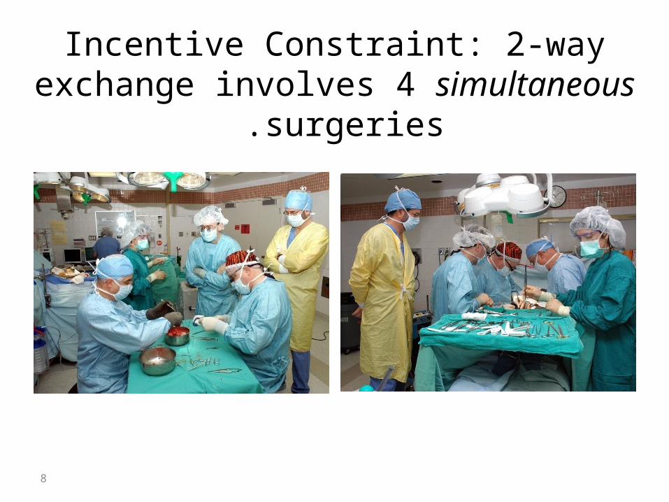
Incentive Constraint: 2-way exchange involves 4 simultaneous surgeries .

9
3-pair exchange (6 simultaneous surgeries)
Donor 1 Recipient 1Pair 1
Donor 2 Recipient 2
Pair 2
Donor 3 Recipient 3
Pair 3
10
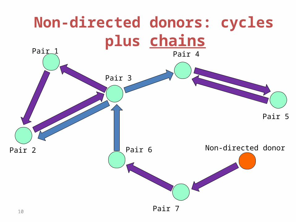
Non-directed donors: cycles plus chains
Pair 1
Pair 2
Pair 3
Pair 4
Pair 6
Pair 7
Pair 5
Non-directed donor
11
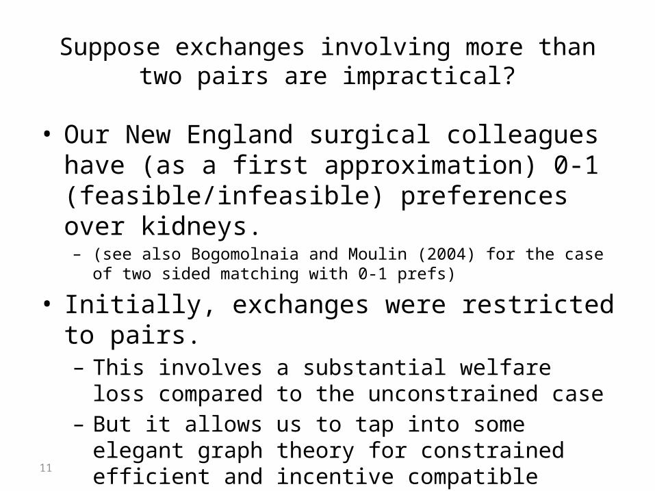
Suppose exchanges involving more than two pairs are impractical?
• Our New England surgical colleagues have (as a first approximation) 0-1 (feasible/infeasible) preferences over kidneys.– (see also Bogomolnaia and Moulin (2004) for the case of two sided matching
with 0-1 prefs)
• Initially, exchanges were restricted to pairs. – This involves a substantial welfare loss compared to the
unconstrained case– But it allows us to tap into some elegant graph theory for
constrained efficient and incentive compatible mechanisms.
12
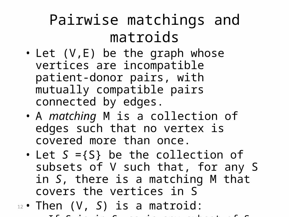
Pairwise matchings and matroids
• Let (V,E) be the graph whose vertices are incompatible patient-donor pairs, with mutually compatible pairs connected by edges.
• A matching M is a collection of edges such that no vertex is covered more than once.
• Let S ={S} be the collection of subsets of V such that, for any S in S, there is a matching M that covers the vertices in S
• Then (V, S) is a matroid:– If S is in S, so is any subset of S.– If S and S’ are in S, and |S’|>|S|, then there is a point
in S’ that can be added to S to get a set in S.
13
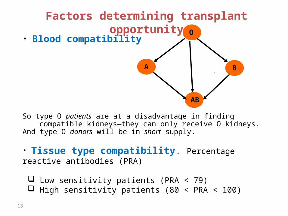
Factors determining transplant opportunity
• Blood compatibility
So type O patients are at a disadvantage in finding compatible kidneys—they can only receive O kidneys.
And type O donors will be in short supply.
• Tissue type compatibility. Percentage reactive antibodies (PRA)
Low sensitivity patients (PRA < 79) High sensitivity patients (80 < PRA < 100)
O
A B
AB

14
A. Patient ABO Blood Type Frequency
O 48.14%
A 33.73%
B 14.28%
AB 3.85%
B. Patient Gender Frequency
Female 40.90%
Male 59.10%
C. Unrelated Living Donors Frequency
Spouse 48.97%
Other 51.03%
D. PRA Distribution Frequency
Low PRA 70.19%
Medium PRA 20.00%
High PRA 9.81%
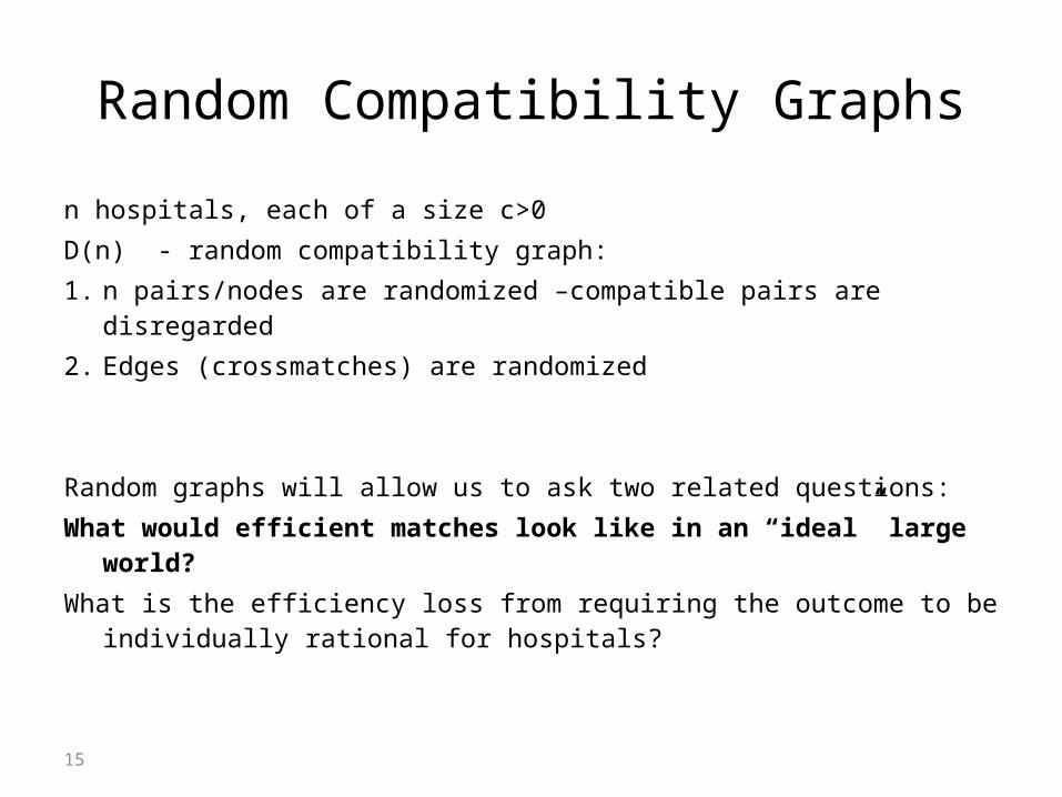
Random Compatibility Graphs
n hospitals, each of a size c>0 D(n) - random compatibility graph:1. n pairs/nodes are randomized –compatible pairs are disregarded2. Edges (crossmatches) are randomized
Random graphs will allow us to ask two related questions:What would efficient matches look like in an “ideal” large world?What is the efficiency loss from requiring the outcome to be
individually rational for hospitals?
15
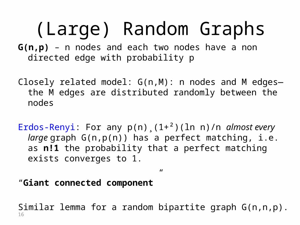
(Large) Random GraphsG(n,p) – n nodes and each two nodes have a non directed edge
with probability p
Closely related model: G(n,M): n nodes and M edges—the M edges are distributed randomly between the nodes
Erdos-Renyi: For any p(n)¸(1+²)(ln n)/n almost every large graph G(n,p(n)) has a perfect matching, i.e. as n!1 the probability that a perfect matching exists converges to 1.
“Giant connected component”
Similar lemma for a random bipartite graph G(n,n,p).16

17
A disconnect between model and data:
• The large graph model with constant p (for each kind of patient-donor pair) predicts that only short chains are useful.
• But we now see long chains in practice.• They could be inefficient—i.e. competing with
short cycles for the same transplants.• But this isn’t the the case when we examine
the data.
18
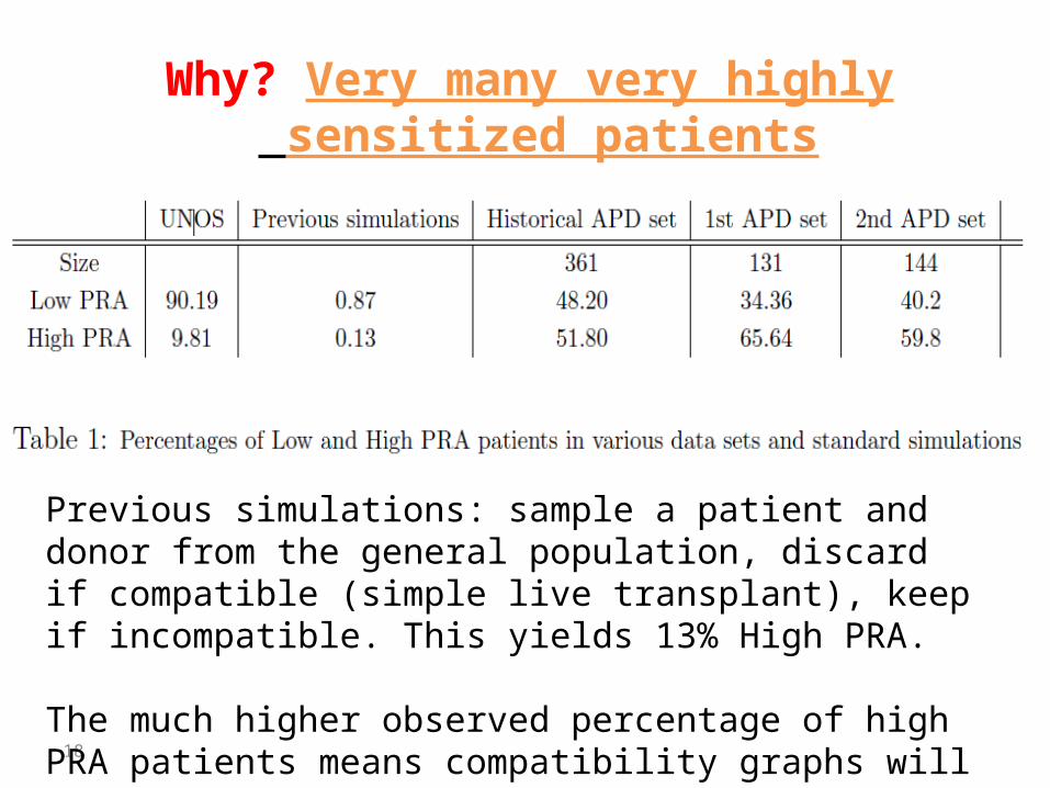
Why? Very many very highly sensitized patients
Previous simulations: sample a patient and donor from the general population, discard if compatible (simple live transplant), keep if incompatible. This yields 13% High PRA.
The much higher observed percentage of high PRA patients means compatibility graphs will be sparse

19
20
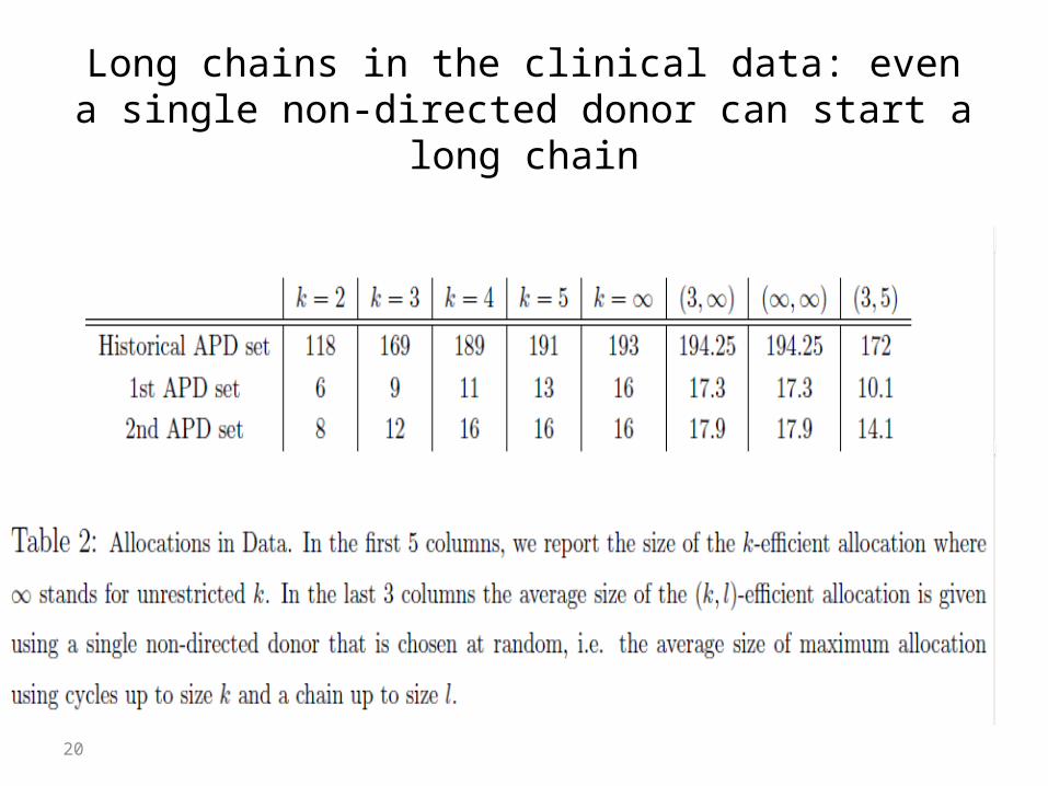
Long chains in the clinical data: even a single non-directed donor can start a long chain
21
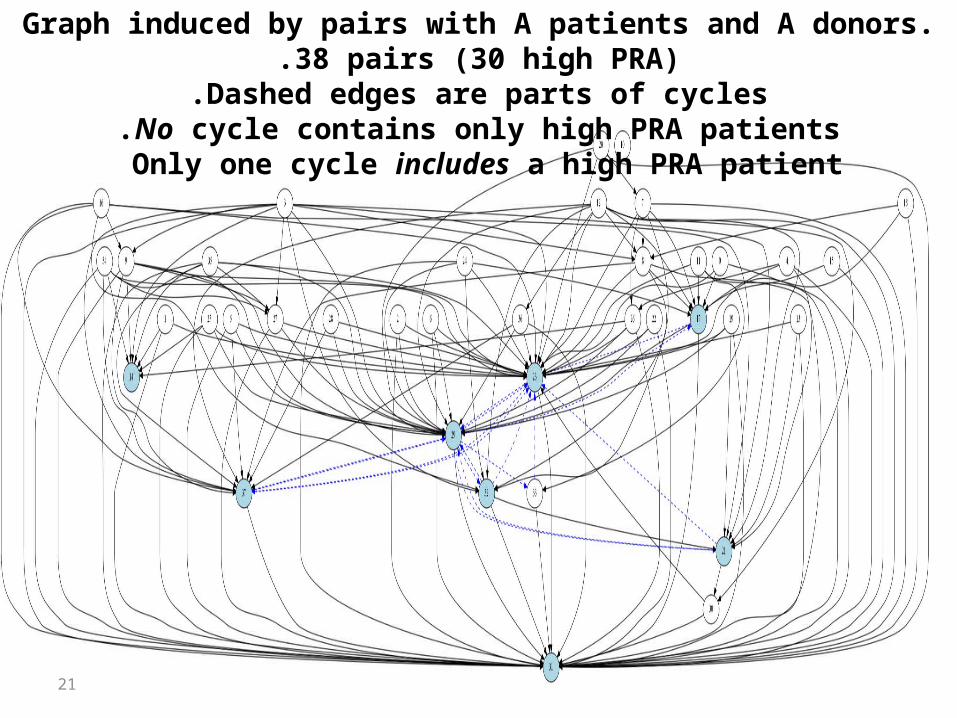
Graph induced by pairs with A patients and A donors. 38 pairs (30 high PRA).Dashed edges are parts of cycles.
No cycle contains only high PRA patients.Only one cycle includes a high PRA patient
22
Jellyfish structure of the compatibility graph: highly connected low sensitized pairs, sparse hi-sensitized pairs
23
So we need to model sparse graphs…• We’ll consider random graphs with two kinds of nodes
(patient-donor pairs): Low sensitized and high sensitized• L nodes will have a constant probability of an incoming edge
(compatible kidney)• H nodes will have a probability that decreases with the size of
the graph (e.g. in a simple case we’ll keep the number of compatible kidneys constant, pH = c/n)
• In the H subgraph, we’ll observe trees but almost no short cycles
• A non-directed donor can be modeled as a donor with a patient to whom anyone can donate—this allows non-directed donor chains to be analyzed as cycles
• (We also consider the effect of different assumptions about how the number of non-directed donors grows…)

Cycles and paths in random dense-sparse graphs
• n nodes. Each node is L w.p. À and H w.p. 1-À
• incoming edges to L are drawn w.p.
• incoming edges to L are drawn w.p.
L
H
25

Cycles and paths in random sparse (sub)graphs (v=0, only highly sensitized patients)
H
Theorem .)a(The number of cycles of length O(1) is O(1) .)b(But when pH is a large constant there is cycle with length O(n)
Proof (a):
26 To be logistically feasible, a long cycle must be a chain, i.e. contain a NDD
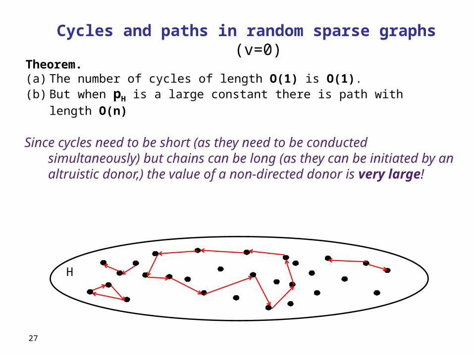
Cycles and paths in random sparse graphs (v=0)
H
Theorem. )a( The number of cycles of length O(1) is O(1). )b( But when pH is a large constant there is path with length O(n)
Since cycles need to be short (as they need to be conducted simultaneously) but chains can be long (as they can be initiated by an altruistic donor,) the value of a non-directed donor is very large!
27

Case v>0 (some low sensitized, easy to match patients. Why increasing cycle size helps
L
H
Theorem. Let Ck be the largest number of transplants achievable with
cycles · k. Let Dk be the largest number of transplants achievable with
cycles · k plus one non-directed donor. Then for every constant k there exists ½>0
Furthermore, Ck and Dk cover almost all L nodes .
28

Case v>0. Why increasing cycle size helps
Increasing cycle lengths significantly increases transplants. Highly sensitized patients are the principal beneficiaries.
Low sensitized pairs of all blood types are overdemanded: it’s easy to start a cycle from L to H since there are many H, and easy to end it back in L since most blood type compatible donors will do…
29

Simulations (re-sampling) with clinical data
30
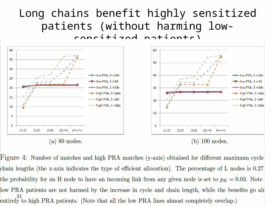
Long chains benefit highly sensitized patients (without harming low-sensitized patients)
31
32
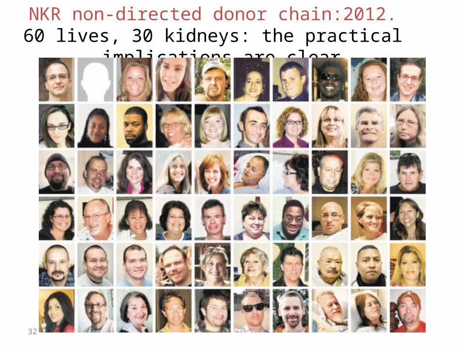
NKR non-directed donor chain:2012. 60 lives, 30 kidneys: the practical implications are clear

How about when hospitals become players?
• We are seeing some hospitals withhold internal matches, and contribute only hard-to-match pairs to a centralized clearinghouse.
• Mike Rees (APD director) writes us: “As you predicted, competing matches at home centers is becoming a real problem. Unless it is mandated, I'm not sure we will be able to create a national system. I think we need to model this concept to convince people of the value of playing together”.
33

No strategy proof mechanism
a1
a2 a3
a4
b3
b2b1
35
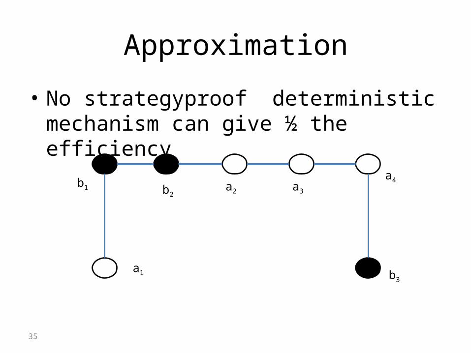
Approximation
• No strategyproof deterministic mechanism can give ½ the efficiency
a1
a2 a3
a4
b3
b2b1
36
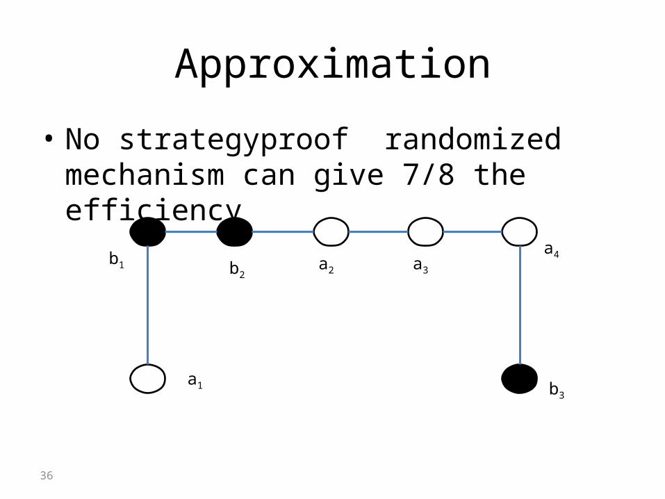
Approximation
• No strategyproof randomized mechanism can give 7/8 the efficiency
a1
a2 a3
a4
b3
b2b1
Individual rationality and efficiency: an impossibility theorem with a (discouraging) worst-
case bound
• For every k> 3, there exists a compatibility graph such that no k-maximum allocation which is also individually rational matches more than 1/(k-1) of the number of nodes matched by a k-efficient allocation.
37
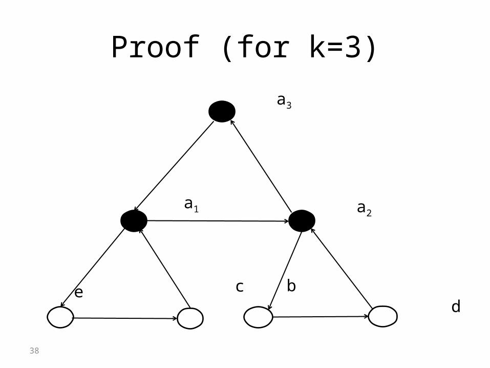
Proof (for k=3)
38
a3
a2
cd
a1
e b

“Cost” of IR is very small - Simulations
No. of Hospitals 2 4 6 8 10 12 14 16 18 20 22
IR,k=3 6.8 18.37 35.42 49.3 63.68 81.43 97.82109.01121.81144.09 160.74
Efficient, k=3 6.89 18.67 35.97 49.75 64.34 81.83 98.07109.41 122.1 144.35 161.07
39
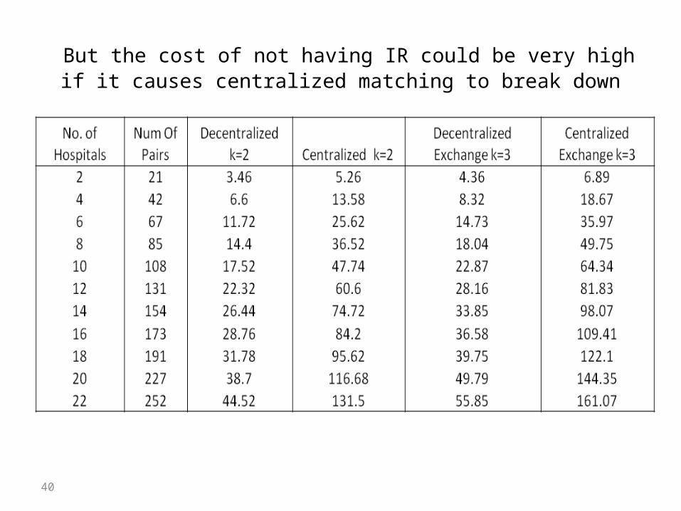
But the cost of not having IR could be very high if it causes centralized matching to break down
40
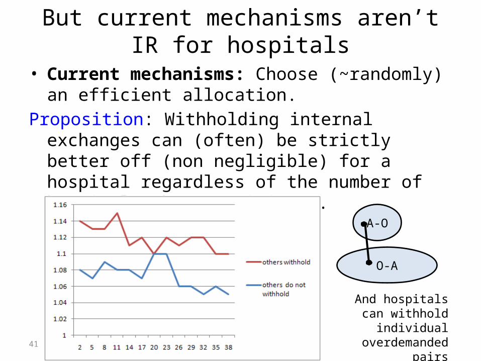
But current mechanisms aren’t IR for hospitals
• Current mechanisms: Choose (~randomly) an efficient allocation.
Proposition: Withholding internal exchanges can (often) be strictly better off (non negligible) for a hospital regardless of the number of hospitals that participate.
O-A
A-O
41
And hospitals can withhold individual
overdemanded pairs
42
What if we have a prior?
• Infinite horizon• In each timestep, a hospital samples its
patients from some known distribution• Then there exists a truthful mechanism with
efficiency 1 – o(1)

43
Matching
• Initially the hospital has zero credits• In the beginning of the round, if the hospital
has zero credits, each patients enters the match with probability 1 – 1/k1/6
• For each positive credit, the hospital increases this probability by 1/k2/3 and the credit is gone
• For each negative credit, the hospital decreases this probability by 1/k2/3 and the credit is gone. The probability is always > ½
44
Gaining credit
• For each patient over k, the hospital gets 1 credit
• For each patient below k, the hospital looses 1 credit
• These credits only affect the next rounds

45
Proof idea
• Hiding a patient can give an additive advantage, but causes a multiplicative loss
• Number of credit doesn’t matter – you always care about the future
• Can work for every distribution of patients
What about dynamics?
What is the tradeoff between waiting and number of matches?
Dynamic matching in dense graphs (Unver, ReStud,2010).
Matching over time
47
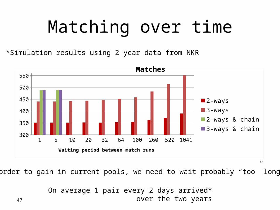
Simulation results using 2 year data from NKR*
In order to gain in current pools, we need to wait probably “too” long
*On average 1 pair every 2 days arrived over the two years
1 5 10 20 32 64 100 260 520 1041300
350
400
450
500
550
2-ways3-ways2-ways & chain3-ways & chain
Waiting period between match runs
Matches

Matching over time
48
Simulation results using 2 year data from NKR*
In order to gain in current pools, we need to wait probably “too” long
*On average 1 pair every 2 days arrived over the two years
Matches – high PRA
1 5 10 20 32 64 100 260 520 104190
110
130
150
170
190
210
230
2-ways3-ways2-ways & chain3-ways & chain
Matching over time
49
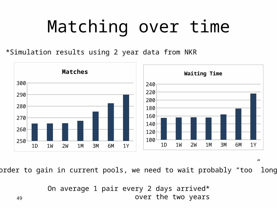
1D 1W 2W 1M 3M 6M 1Y250255260265270275280285290295
Matches
Simulation results using 2 year data from NKR*
1D 1W 2W 1M 3M 6M 1Y100
120
140
160
180
200
220
240
Waiting Time
In order to gain in current pools, we need to wait probably “too” long
*On average 1 pair every 2 days arrived over the two years
50
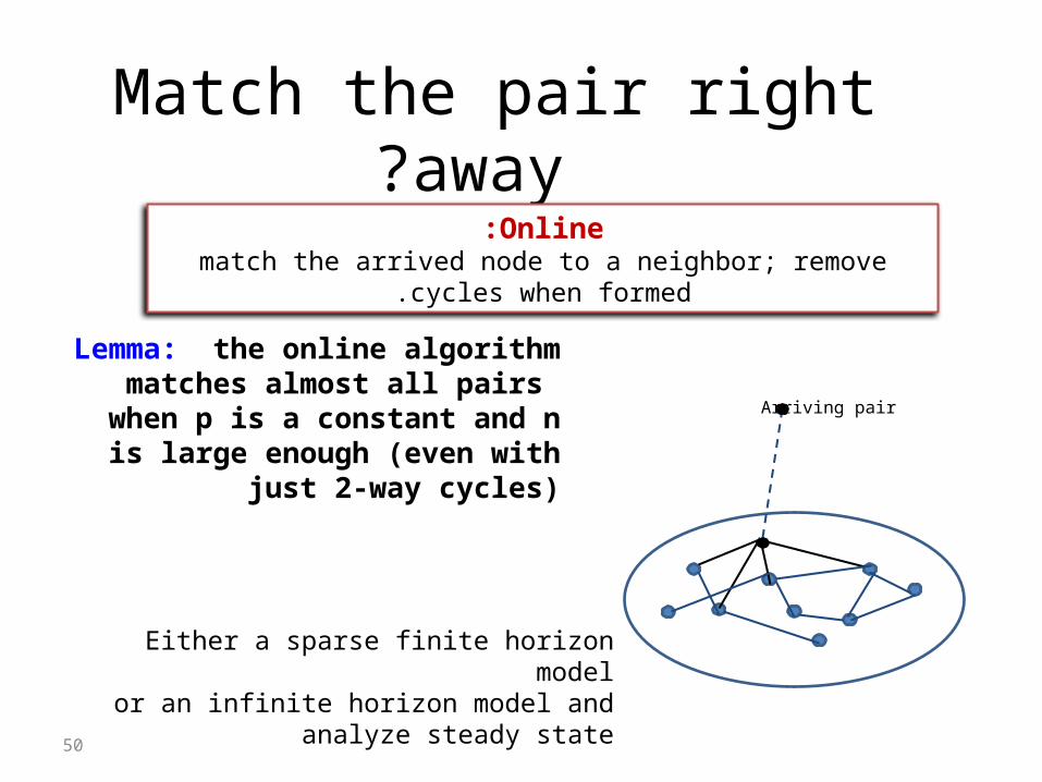
Match the pair right away?
A H-node forms an edge with each node u of U with probability ξ/n. A L-node forms an edge with each node u of U with probability π
Arriving pair
Lemma: the online algorithm matches almost all pairs when p is a constant
and n is large enough (even with just 2-way cycles)
Online:match the arrived node to a neighbor; remove cycles when formed.
Either a sparse finite horizon modelor an infinite horizon model and analyze steady
state
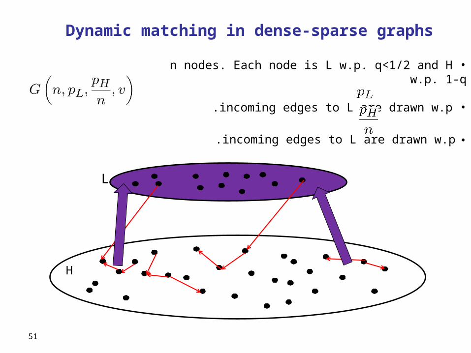
Dynamic matching in dense-sparse graphs
• n nodes. Each node is L w.p. q<1/2 and H w.p. 1-q
• incoming edges to L are drawn w.p .
• incoming edges to L are drawn w.p .
L
H
51

Dynamic matching in dense-sparse graphs
• n nodes. Each node is L w.p. q<1/2 and H w.p. 1-q
• incoming edges to L are drawn w.p .
• incoming edges to L are drawn w.p .
L
H
52
At each time step 1,2,…, n, one node arrives .
53
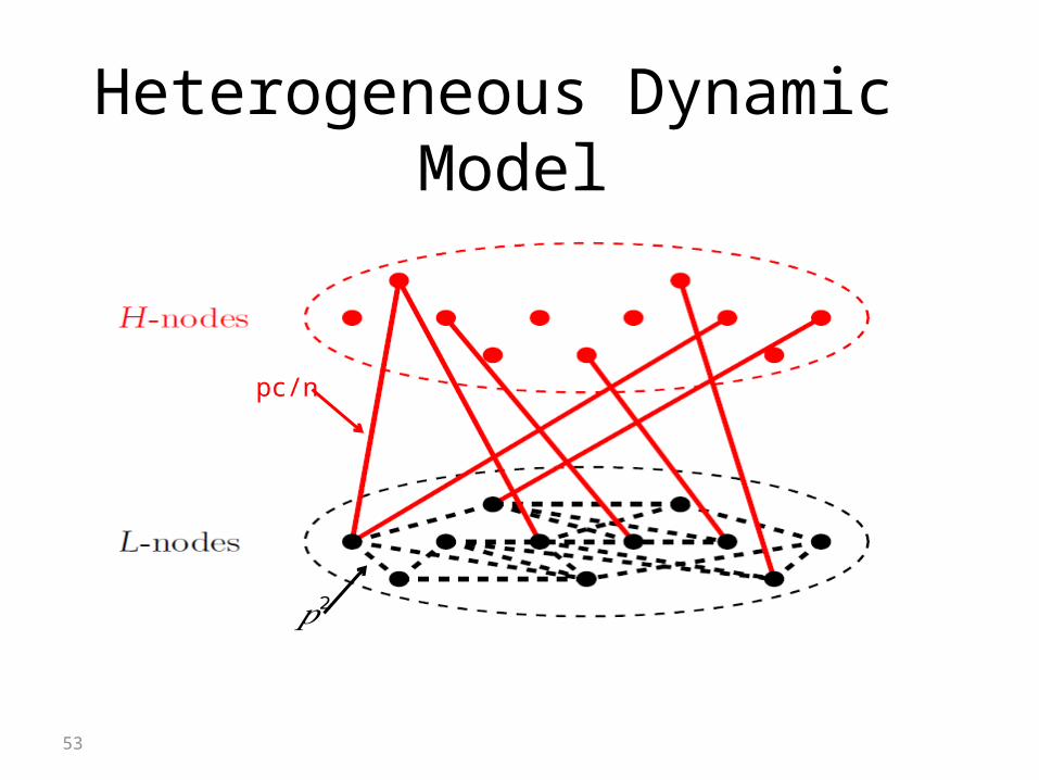
Heterogeneous Dynamic Model (PRA). PRA determines the likelihood that a patient cannot
receive a kidney from a blood-type compatible donor. PRA < 79: Low sensitivity patients (L-patients). 80 < PRA < 100: High sensitivity patients (H-patients).
Most blood-type compatible pairs that join the pool have H-patients. Distribution of High PRA patients in the pool is different from the population PRA.
pc/n
𝑝2
54
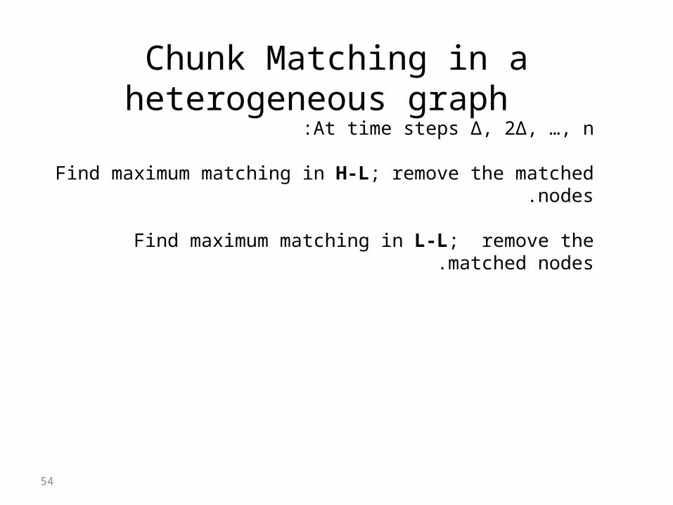
Chunk Matching in a heterogeneous graph At time steps Δ, 2Δ, …, n:
Find maximum matching in H-L; remove the matched nodes.
Find maximum matching in L-L; remove the matched nodes.
55
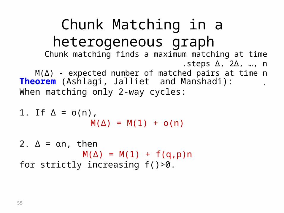
Chunk Matching in a heterogeneous graph
Theorem (Ashlagi, Jalliet and Manshadi): When matching only 2-way cycles:
1. If Δ = o(n), M(Δ) = M(1) + o(n)
2. Δ = αn, then M(Δ) = M(1) + f(q,p)n
for strictly increasing f()>0.
Chunk matching finds a maximum matching at time steps Δ, 2Δ, …, n.M(Δ) - expected number of matched pairs at time n
.
56
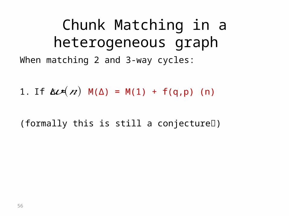
Chunk Matching in a heterogeneous graph
When matching 2 and 3-way cycles:
1. If Δ = M(Δ) = M(1) + f(q,p) (n)
(formally this is still a conjecture)
𝜔 (𝑛)
57
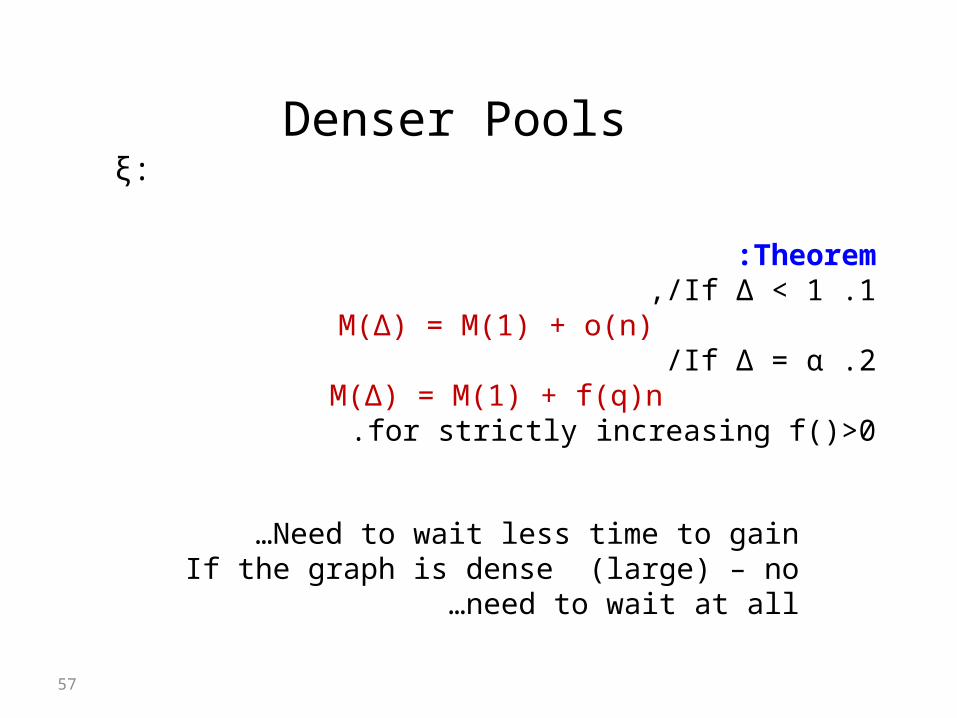
Denser Poolsξ:
Theorem: 1 .If Δ < 1 ,/
M(Δ) = M(1) + o(n)2 .If Δ = α/
M(Δ) = M(1) + f(q)nfor strictly increasing f()>0.
Need to wait less time to gain …If the graph is dense (large) – no need to wait at all…

58
Special structure: Sparse H-L and dense L-L.
(PRA). PRA determines the likelihood that a patient cannot receive a kidney from a
blood-type compatible donor. PRA < 79: Low sensitivity patients (L-patients). 80 < PRA < 100: High sensitivity patients (H-patients).
Most blood-type compatible pairs that join the pool have H-patients. Distribution of High PRA patients in the pool is different from the population PRA.
Compare the number of H-L matchings.
Proof Ideas
pξ/n
𝑝2
59
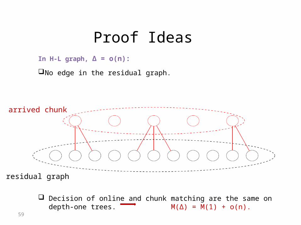
In H-L graph, Δ = o(n):
No edge in the residual graph.
Tissue-type compatibility: Percentage Reactive Antibodies (PRA). PRA determines the likelihood that a patient cannot receive a kidney from a blood-type
compatible donor. PRA < 79: Low sensitivity patients (L-patients). 80 < PRA < 100: High sensitivity patients (H-patients).
Most blood-type compatible pairs that join the pool have H-patients. Distribution of High PRA patients in the pool is different from the population PRA.
Decision of online and chunk matching are the same on depth-one trees. M(Δ) = M(1) + o(n).
arrived chunk
residual graph
Proof Ideas

60
In H-L graph, Δ = αn: Find f(α)n augmenting paths to the matching obtained by online. Given M the matching of the online scheme:
Chunk matching would choose (l1,h1) and (l2,h2). M(Δ) = M(1) + f(α)n,
Proof Ideas
h1
l2 l1
h2

61
Chunk Matching in a heterogeneous graph
Theorem (Ashlagi, Jalliet and Manshadi):
MC(1) = M(1) + f(q)n
M(Δ) - expected number of matches using only 2-ways MC(Δ) - expected number of using 2-ways and allowing an unbounded chain
.