mechanism design without revenue...
TRANSCRIPT
Mechanism Design Without Revenue Equivalence∗
Juan Carlos Carbajal†
School of EconomicsUniversity of Queensland
Jeffrey Ely‡
Department of EconomicsNorthwestern University
October 18, 2010
Abstract
We characterize incentive compatible mechanisms in quasi-linear environmentswhere the envelope theorem and revenue equivalence fail due to non-convex andnon-differentiable valuations. Despite these obstacles, we obtain a characterizationbased on the familiar Mirrlees representation of the indirect utility and a mono-tonicity condition on the allocation rule. These conditions pin down the range ofpossible payoffs as a function solely of the allocation rule, thus providing a rev-enue inequality. We use our characterization in two economic applications wherestandard techniques based on revenue equivalence fail. We find a budget-balancedefficient mechanism in a public goods setting, and we characterize the optimal sell-ing mechanism when the buyer has loss-averse preferences a la Koszegi and Rabin(2006).
Keywords: Incentive Compatibility, Revenue Equivalence, Integral Monotonicity,Subderivative Correspondence, Budget Balancedness, Revenue Maximization.
JEL Classification Numbers: C72, D70, D82, D44.
∗A previous version of this paper (with different title) was presented at the Game Theory Festival 2010(Stony Brook) and SAET 2010 (Singapore). The first author is indebted to Claudio Mezzetti and AndrewMcLennan for helpful discussions. We also thank comments by Benny Moldovanu, Ahuva Mu’alem,Rudolf Muller and Rakesh Vohra.
†Email address: [email protected].‡Email address: [email protected].
1
1 Introduction
Revenue equivalence states that, under certain conditions, two (dominant strategy1)incentive compatible mechanisms with the same allocation rule generate utilities forthe agent and payments to the planner that differ at most by a constant. The revenueequivalence principle is very useful in simplifying mechanism design problems in avariety of settings, as first shown by Myerson (1981). A large literature studies thebreadth of conditions under which revenue equivalence holds.2
In this paper, we characterize incentive compatibility in the absence of linearity, con-vexity and differentiability assumptions on the valuation function with respect to types.Without these assumptions, revenue equivalence as traditionally formulated may failbut the range of potential payoffs can still be determined. Moreover, our characteriza-tion can be employed analogously to the traditional one in various applications such asefficient, budget-balancing, and revenue-maximizing mechanism design.
The following simple example illustrates these ideas.
Example 1. The allocation set is X = [0, 1]. The agent has a quasi-linear utility functionu = v(x, θ)− ρ defined over alternatives x ∈ X and monetary payments ρ ∈ R. Typesare private information and lie in Θ = [0, 1]. The agent’s valuation function v : X ×Θ→ R is given by
v(x, θ) =
{θx, if x ≤ θ;2θ2 − θx, if x > θ.
Think of x as the quantity traded of some good. Our agent has positive marginal utilityfor the first θ units, and negative marginal utility for additional amounts. Note thatfor each x, the function θ 7→ v(x, θ) is neither convex nor fully differentiable on Θ. Inparticular, its partial derivative with respect to θ fails to exist whenever θ = x.
The efficient allocation rule X∗ : Θ → X selects X∗(θ) = θ. Clearly X∗ is imple-mentable, indeed by a constant payment rule p ≡ 0. In this case, the direct mechanism(X, p) generates zero revenue and an indirect utility function for the agent given by
U(θ) = v(X∗(θ), θ)− p(θ) = θ2.
However, revenue equivalence fails. For example, consider the alternative paymentrule p′ defined by p′(θ) = θ2/2, all θ ∈ Θ. To see that the mechanism (X∗, p′) is
1We study single-agent, dominant strategy incentive compatible mechanisms. This is for expositionalclarity. It is straightforward to generalize our results to many agents and to Bayesian incentive compati-bility.
2Berger, Muller, and Naeemi (2010) build on the envelope theorem of Milgrom and Segal (2002) toestablish revenue equivalence when the type space is a convex subset of a multi-dimensional Euclideanspace and valuations are convex or differentiable in types. See also Krishna and Maenner (2001), Jehiel,Moldovanu, and Stacchetti (1996, 1999), Williams (1999), Heydenreich, Muller, Uetz, and Vohra (2009) andChung and Olszewski (2007). Holmstrom (1979) and Carbajal (2010) develop an alternative method torevenue equivalence for efficient allocation rules.
2
incentive compatible, fix a type θ ∈ Θ. Reporting θ ∈ Θ generates payoffs equal to
v(X∗(θ), θ) − p′(θ) =
{θθ − θ2/2, if θ ≤ θ;2θ2 − θθ − θ2/2, if θ > θ.
The above expression is maximized when θ = θ. In this mechanism, type θ = 0 obtainszero utility, just as in (X∗, p), and yet (X∗, p′) generates strictly positive revenues andan indirect utility function U′ given by U′(θ) = θ2/2. �
We shall see that despite the failure of revenue equivalence, the full set of incentivecompatible payment rules can be characterized by versions of standard conditions. Ap-plied to Example 1, we can show that U is an indirect utility function arising from anincentive compatible mechanism with the allocation rule X∗ if, and only if,
U(θ) = U(0) +∫ θ
0s(θ) dθ, for all θ ∈ Θ, (1)
for some function θ 7→ s(θ) such that
s is an integrable selection from the correspondence S(θ) = [θ, 3θ] (2)
satisfying, for all θ, θ ∈ Θ,
v(X∗(θ), θ)− v(X∗(θ), θ) ≥∫ θ
θs(θ) dθ ≥ v(X∗(θ), θ)− v(X∗(θ), θ). (3)
Equation 1 is the familiar Mirrlees representation of incentive compatible payoffs.Equation 2 generalizes the standard envelope theorem derivation of the integrand θ 7→s(θ). In models with differentiable valuations, s(θ) would be given by the partialderivative of v(X∗(θ), θ) with respect to its second argument evaluated at θ = θ. Thisrequirement is modified to allow s(θ) to range between the right and left subderiva-tives3 of v(X∗(θ), θ) at θ = θ, which in this case are θ and 3θ, respectively. Finally, asis always the case, some form of monotonicity of the allocation rule is necessary forincentive compatibility. Here Equation 3, the integral monotonicity condition, turns out tobe necessary and, together with the previous two conditions, sufficient.4
Our main result, Theorem 1, extends this characterization to a general mechanismdesign setting with utilities that are quasi-linear in money, a convex, possibly multi-dimensional type space, and a measurable space of outcomes. In place of differentiabil-ity, convexity, or absolute continuity, we assume that the valuation function satisfiesa uniform Lipschitz condition with respect to types. This condition, along with an
3Mathematical concepts and results are presented in Section 2.2.4This condition is also studied in Berger, Muller, and Naeemi (2010) who characterize incentive com-
patibility in settings where revenue equivalence holds.
3
additional technical restriction, allows us to employ integrable selections of the sub-derivative correspondence (cf. Equation 2) in place of the usual envelope derivation. Inmulti-dimensional settings, a closed-path integrability condition appears in our char-acterization of incentive compatible mechanisms, in addition to the three conditionsmentioned above.
In Section 5 we apply our characterization result to two settings: an efficient publicgood provision problem, and the design of an optimal selling mechanism when buyersare loss-averse. It is well understood that when revenue equivalence holds, the efficientallocation rule is implementable if and only if it is implementable via a Vickrey-Clarke-Groves (VCG) payment rule. We consider a location model for a public good whererevenue equivalence fails and show that, in this case, efficient allocations can be im-plemented with a budget-balanced payment rule, and yet no VCG mechanism has abalanced budget. In the buyer-seller model, the buyer has loss-averse preferences a laKoszegi and Rabin (2006) which, due to a kink on the valuation at the reference point,fails standard requirements of differentiability or convexity. Nonetheless, our charac-terization result applies and allows us to expand Myerson’s (1981) techniques to thissituation, thus reformulating the seller’s problem in terms of virtual valuations. Inthe optimal selling mechanism, a range of intermediate types purchase their referencequantity so that the flexibility of pricing rules afforded by our characterization plays animportant role. Compared to the case without loss aversion, some of these intermedi-ate types have their quantities distorted downward to exploit the loss aversion of evenhigher types, whose incentive constraints are thereby slackened and their paymentscorrespondingly increased. Similarly, the loss aversion of lower intermediate types isexploited by making them pay a premium to increase their quantity from zero to theirreference points.
In Section 4 we derive a revenue inequality in the spirit of the standard revenue equiv-alence principle. Our Theorem 2 shows that, after normalizing the utility of the “low-est type”, the difference in equilibrium payoffs generated by two incentive compatiblemechanisms with the same allocation rule is bounded, with bounds depending solelyon the allocation rule. Using our version of the Mirrlees representation of indirect util-ities, we are able to show that any payment rule used to implement an allocation rulehas a simple representation based on the subderivative correspondence. It follows thatthe set of normalized equilibrium payoffs is convex: if two payment rules implementan allocation rule and generate indirect utility functions U and U′, respectively, then forevery convex combination Uλ of U and U′ there exists a payment function that imple-ments the allocation rule and generates an indirect utility equal to Uλ.
In Section 6, we relate our approach to previous work and show that, with the in-clusion of a minor measurability hypothesis on the right and left subderivatives of thevaluation function, our characterization result is obtained whenever the valuation is ei-ther convex, concave, or differentiable with respect to types. We also show that revenueequivalence is restored when valuations are convex or differentiable, or whenever the
4
allocation set is finite. Section 7 ends this paper with some concluding remarks.
1.1 Related Literature
Integral monotonicity is connected to the variety of monotonicity conditions studied inthe literature since Rochet (1987), who characterized incentive compatibility via cyclicmonotonicity. Saks and Yu (2005), Bikhchandani, Chatterji, Lavi, Mu’alem, Nisan,and Sen (2006), and Ashlagi, Braverman, Hassidim, and Monderer (2010) investigateweaker forms of monotonicity in environments with finitely many allocations. For infi-nite allocation sets, Archer and Kleinberg (2008) extend the insights of Jehiel, Moldovanu,and Stacchetti (1999) and characterize implementable allocation rules via weak mono-tonicity (plus a closed-path integrability condition) in environments with multi-dimensionalconvex type spaces and valuations that are linear in types. In independent work, Berger,Muller, and Naeemi (2010) study environments with convex or differentiable valuationsand obtain a characterization of incentive compatibility using integral monotonicity(which they call path monotonicity).
We recently became aware of independent work by Kos and Messner (2010) andRahman (2010) who also characterize incentive compatibility in general settings. Rah-man (2010) uses linear programming and duality to characterize incentive compatibleallocations in terms of detectable deviations. Kos and Messner (2010) takes a perspec-tive that is more similar to ours, studying the extremal transfer rules that implementan allocation. Relative to both of these papers, we impose additional structure (notablyLipschitz continuity) and in return obtain characterizations which are more immedi-ately suitable for applications. We demonstrate two such applications in Section 5.
2 Preliminaries
2.1 The design setting
We consider a single-agent mechanism design setting; extensions to multi-agent set-tings are straightforward. An outcome (x, ρ) is composed of an alternative x that be-longs to the allocation set X , and a real number ρ representing some quantity of a per-fectly divisible commodity (money). Our agent has quasi-linear preferences, so that
u(x, θ, ρ) = v(x, θ) − ρ
represents the agent’s utility when x ∈ X is selected and amount ρ ∈ R is paid, givenher privately known type θ. We denote the agent’s type space by Θ and refer to v : X ×Θ→ R as the valuation function.
The following assumptions are made throughout this paper.
(A1) The pair (X ,M) is a measurable space (M denotes a σ-algebra of subsets of X ).
5
(A2) The type space Θ is a convex, bounded subset of Rk (k ≥ 1).
(A3) For every x ∈ X , the function θ 7→ v(x, θ) is Lipschitz continuous on Θ: there is apositive number `(x) such that |v(x, θ) − v(x, θ)| ≤ `(x) ‖θ − θ‖, for all θ, θ ∈ Θ.Moreover, { `(x) | x ∈ X } is bounded above, with ` = sup{ `(x) | x ∈ X } < +∞.
(A1) does not impose any burdensome restriction on the allocation set, which couldbe finite or infinite. The convexity of the type space in (A2) is a standard assumptionand is satisfied in several economic applications.5 (A3) is used to prove the Lipschitzcontinuity of the indirect utility function. It is not possible to dispense with the bound-edness assumption on the set of Lipschitz constants when X is infinite.6 In addition,(A3) allows us to work with the right and left subderivatives of the valuation functionwith respect to types.
We consider direct mechanisms of the form (X, p), where the function X : Θ→ X iscalled the allocation rule and the function p : Θ → R is called the payment rule. X is saidto be implementable if there exists a payment rule p such that truth-telling is an dominantstrategy for the agent; i.e.,
v(X(θ), θ) − p(θ) ≥ v(X(θ), θ) − p(θ), for all θ, θ ∈ Θ. (4)
In that case the direct mechanism (X, p) is said to be incentive compatible and the functionU : Θ→ R defined by
U(θ) ≡ v(X(θ), θ) − p(θ), all θ ∈ Θ, (5)
is called the indirect utility generated by (X, p). We shall restrict our analysis to measur-able allocation rules.
2.2 Subderivatives and the integral of a correspondence
We introduce some concepts and results that are later used in our characterization the-orem. The reader is referred to Aubin and Frankowska (1990), Hildenbrand (1974) andRockafellar and Wets (1998) for details.
Fix x ∈ X , θ ∈ Θ, and let δ ∈ Rk, δ 6= 0, be a directional vector for which θ + rδ ∈ Θfor a sufficiently small scalar r. The right and left subderivatives of the function θ 7→
5At some notational cost, one could instead assume that Θ is polygonally connected. The boundednessof the type space plays a technical role in some of our results.
6The following well-known example illustrates this point. Let X = N, Θ = [0, 1], and f : N×Θ → R
be defined by
f (n, θ) =
{1, if 0 ≤ θ ≤ 1− 1
n ;n(1− θ), if 1− 1
n < θ ≤ 1.
For each n ∈N, θ 7→ f (n, θ) is Lipschitz on Θ with `(n) = n. However, the function g : Θ→ R defined byg(θ) = supn∈N f (n, θ), all θ ∈ Θ, is clearly discontinuous at θ = 1.
6
v(x, θ) evaluated at θ ∈ Θ in the direction δ are defined, respectively, as the followinglower and upper limits:
dv(x, θ; δ) ≡ lim infr↓0
v(x, θ + rδ)− v(x, θ)
r; (6)
dv(x, θ; δ) ≡ lim supr↑0
v(x, θ + rδ)− v(x, θ)
r. (7)
By (A3), these subderivatives exist and are finite. Note that dv(x, θ; δ) = −dv(x, θ;−δ).If θ 7→ v(x, θ) admits one-sided directional derivatives at θ, then one can replace theupper and lower limits in (6) and (7) with the usual one-sided limits, although theabove notation is maintained.
Given types θ1, θ2 in Θ, denote their vector difference by δ21 ≡ θ2 − θ1. The open
line segment connecting θ1 to θ2 is the set L(θ1, θ2) = { θ1 + α δ21 | α ∈ (0, 1) }. By (A2),
one has L(θ1, θ2) ⊆ Θ for all θ1, θ2 ∈ Θ. We shall make implicit use of the functionα 7→ θ2
1(α) ≡ θ1 + α δ21 mapping (0, 1) onto L(θ1, θ2).
Let B(0, 1) denote the Borel σ-algebra of subsets of (0, 1). Let S : (0, 1) ⇒ R be acorrespondence with closed images. Then S is said to be a measurable correspondenceif for every open set O in R, the inverse image S−1(O) = { α ∈ (0, 1) | S(α) ∩O 6= ∅ }belongs to B(0, 1). In particular, dom S = { α ∈ (0, 1) | S(α) 6= ∅ } and its complementare measurable sets. S is said to be integrably bounded if there exists a non-negative(Lebesgue) integrable function g defined on (0, 1) such that S(α) ⊆ [− g(α), g(α)] foralmost all α in (0, 1). A selection s of the correspondence S is a function α 7→ s(α) suchthat s(α) ∈ S(α), a.e. in (0, 1). By the Measurable Selection Theorem, a measurable cor-respondence S : (0, 1) ⇒ R admits a measurable selection s : (0, 1) → R. If in additionS is integrably bounded, then it admits (Lebesgue) integrable selections. In such case,Aumann’s (1965) integral of the correspondence S is the non-empty set{ ∫ 1
0s(α) dα | s(α) ∈ S(α) a.e. in (0, 1)
}.
By the Lyapunov’s Convexity Theorem, the integral of a closed-valued, measurable andintegrably bounded correspondence S : (0, 1) ⇒ R is a non-empty closed interval.
3 Characterizing incentive compatible mechanisms
Consider a direct mechanism (X, p). We start with the following observation: if (X, p)is incentive compatible, then its associated indirect utility is Lipschitz continuous on Θand has two-sided directional derivatives a.e. in the line segment connecting any twotypes.
7
Lemma 1. Assume that (A1) to (A3) are satisfied, and let p : Θ→ R implement the allocationrule X. The following statements hold:
(a) The indirect utility function U generated by (X, p) is Lipschitz continuous on Θ.
(b) For every pair θ1, θ2 of distinct types in Θ, U admits two-sided directional derivatives inthe direction δ2
1 = θ2 − θ1 a.e. in L(θ1, θ2).
Proof (a) Consider arbitrary types θ1, θ2 in Θ. From Equation 4 and Equation 5 onesees that
U(θ2)−U(θ1) ≤{
v(X(θ2), θ2)− p(θ2)}−{
v(X(θ2), θ1)− p(θ2)}
= v(X(θ2), θ2) − v(X(θ2), θ1) ≤ `(X(θ2)) ‖θ2 − θ1‖ ≤ ` ‖θ2 − θ1‖;
where the last two inequalities follow from (A3). Reversing the roles of θ1 and θ2, onereadily concludes that |U(θ2)−U(θ1)| ≤ `‖θ2 − θ1‖, as desired.
(b) Fix distinct types θ1, θ2 in Θ. Define the function µ on (0, 1) by µ(α) = U(θ21(α)),
where θ21(α) ≡ θ1 + α δ2
1 ∈ L(θ1, θ2). It is readily seen that µ is Lipschitz continuous.Indeed, for any 0 < α, α′ < 1, one has:
|µ(α)− µ(α′)| = |U(θ21(α))−U(θ2
1(α′))| ≤ ` ‖θ2
1(α)− θ21(α′)‖ = ` ‖δ2
1‖ |α− α′|,
with the above inequality following from part (a). Thus, µ is Lipschitz and thereforeabsolutely continuous and differentiable a.e. in (0, 1). In particular, if µ is differentiableat α ∈ (0, 1), then we deduce:
Dµ(α) = limr→0
µ(α + r)− µ(α)
r= lim
r→0
U(θ21(α) + r δ2
1)−U(θ21(α))
r= DU(θ2
1(α); δ21),
with last term above denoting the two-sided directional derivative of U at θ21(α) in the
direction δ21 . �
Milgrom and Segal (2002) obtained an analogue of Lemma 1-(a) under the alterna-tive hypothesis of absolute continuity of v(x, ·) on a one-dimensional type space, plusan integral bound condition on the derivative of v with respect to types. The exten-sion of the absolute continuity concept to multi-dimensional settings is not straightfor-ward.7 On the other hand, Lipschitz continuity extends naturally to multi-dimensionaldomains and allows us to work with right and left subderivatives.
We mention that, in multi-dimensional settings, Lemma 1-(b) does not imply that Uis fully differentiable a.e. in the line connecting θ1 and θ2. In fact, there may be many(piecewise) smooth paths between θ1 and θ2 for which U is nowhere fully differentiable
7For instance, it is possible to construct a convex function on a plane that fails to be absolutely continu-ous; see Friedman (1940) for details.
8

in such paths.8 What Lemma 1-(b) states is that the indirect utility generated by anincentive compatible mechanism admits two-sided directional derivatives in the direc-tion δ2
1 a.e. in L(θ1, θ2). We use this fact to derive a relationship between the right andleft subderivatives of the valuation function at equilibrium points. Define the right andleft subderivative functions between θ1 and θ2, respectively, by
s(θ21(α)) ≡ dv(X(θ2
1(α)), θ21(α); δ2
1), all α ∈ (0, 1), (8)
ands(θ2
1(α)) ≡ dv(X(θ21(α)), θ2
1(α); δ21), all α ∈ (0, 1). (9)
The following technical assumption is required in our characterization of incentivecompatible mechanisms.
(M) Given an allocation rule X : Θ→ X , for every pair of distinct types θ1, θ2 ∈ Θ, the rightand left subderivative functions α 7→ s(θ2
1(α)) and α 7→ s(θ21(α)) between θ1 and θ2 are
B(0, 1)-measurable.
Our assumption (M), which is stated in terms of the valuation function and theallocation rule, may be easily verified in some circumstances (cf. Example 1, where fortypes θ ∈ Θ = [0, 1], dv(X∗(θ), θ) = θ and dv(X∗(θ), θ) = 3θ). In Section 6 we showthat (M) is satisfied in settings commonly employed in economic applications.
Using Equation 8 and Equation 9, we construct the subderivative correspondence S(θ2
1(·))
: (0, 1) ⇒R between θ1 and θ2 as follows:
S(θ2
1(α))≡{
r ∈ R | s(θ21(α)) ≤ r ≤ s(θ2
1(α))}
, α ∈ (0, 1). (10)
S(θ2
1(α))
is empty-valued if s(θ21(α)) > s(θ2
1(α)). Whenever the opposite inequalityholds, S
(θ2
1(α))
contains all the real numbers between the right and left subderiva-tive of v with respect to types in the direction δ2
1 , evaluated at (X(θ21(α)), θ2
1(α)).9 The
subderivative correspondence between θ1 and θ2 is said to be regular if it is non empty-valued a.e. in (0, 1), closed-valued, measurable and integrably bounded.
Lemma 2. Assume that (A1) to (A3) and (M) are satisfied. If X is implementable, then for allθ1, θ2 ∈ Θ, θ1 6= θ2, the subderivative correspondence S
(θ2
1(·))
between θ1 and θ2 is regular.
Proof Suppose that p : Θ → R implements X. Fix arbitrary types θ1, θ2 ∈ Θ, θ1 6= θ2.For every θ2
1(α) ∈ L(θ1, θ2), for any scalar r sufficiently small, the indirect utility U
8See Krishna and Maenner (2001) for an example.9Observe S
(θ1
2(α))= − S
(θ2
1(1− α)), all α ∈ (0, 1).
9
generated by (X, p) satisfies
U(θ21(α) + r δ2
1) − U(θ21(α)) ≥ v(X(θ2
1(α)), θ21(α) + r δ2
1) − p(θ21(α))
− v(X(θ21(α)), θ2
1(α)) + p(θ21(α))
= v(X(θ21(α)), θ2
1(α) + r δ21) − v(X(θ2
1(α)), θ21(α)).
If r > 0 then it follows from the above expression that
v(X(θ21(α)), θ2
1(α) + r δ21)− v(X(θ2
1(α)), θ21(α))
r≤ U(θ2
1(α) + r δ21)−U(θ2
1(α))
r, (11)
whereas if r < 0 we have instead
U(θ21(α) + r δ2
1)−U(θ21(α))
r≤ v(X(θ2
1(α)), θ21(α) + r δ2
1)− v(X(θ21(α)), θ2
1(α))
r. (12)
By Lemma 1-(b), U admits two-sided directional derivatives in the direction δ21 a.e. in
L(θ1, θ2). Thus, taking the lower limit as r ↓ 0 in (11) and the upper limit as r ↑ 0 in (12),we infer that a.e. in (0, 1) the following holds:
s(θ21(α)) ≤ DU(θ2
1(α); δ21) ≤ s(θ2
1(α)). (13)
This shows that S(θ2
1(α))6= ∅ a.e. in (0, 1), as desired.
S(θ2
1(·))
is closed-valued by definition. To show that it is measurable, define thecorrespondence T : (0, 1) ⇒ R by T(α) = {s(θ2
1(α))} ∪ {s(θ21(α))} when Equation 13
is satisfied, and T(α) = ∅, otherwise. Since the set { α ∈ (0, 1) | T(α) = ∅ } haszero measure, we deduce from (M) that T is a measurable correspondence, and sois its convex hull conv(T) = S
(θ2
1(·)).10 Further, notice that by (A2) Θ is bounded
and that for every x ∈ X , (A3) implies that |dv(x, θ21(α); δ2
1)| ≤ `‖δ21‖ and similarly
|dv(x, θ21(α); δ2
1)| ≤ `‖δ21‖, for all α ∈ (0, 1). Hence, S
(θ2
1(·))
is integrably bounded. �
The integral of the regular correspondence S(θ2
1(·))
is a non-empty, closed interval.In particular, s(θ2
1(·)) and s(θ21(·)) are integrable selections, with the inequalities∫ 1
0s(θ2
1(α)) dα ≤∫ 1
0s(θ2
1(α)) dα ≤∫ 1
0s(θ2
1(α)) dα
valid for any integrable selection s(θ21(·)) of S
(θ2
1(·)). We use this fact in our character-
ization result. Given any subset {θ1, θ2, θ3} of Θ, denote δmn ≡ θm − θn for n, m = 1, 2, 3.
It is understood that s(θmn (·)) = s(θm
n (·)) ≡ 0 whenever θn = θm.
10Here we use two facts: (i) the union of measurable correspondences is measurable; (ii) the convex hullof a measurable correspondence is also measurable. See the references given in Section 2.2.
10
Theorem 1. Assume (A1) to (A3) are satisfied. Suppose that (M) holds for X : Θ → X . Thefollowing statements are then equivalent.
(a) The allocation rule X : Θ→ X is implementable, with indirect utility function U.
(b) For every subset {θ1, θ2, θ3} of Θ, the subderivative correspondence S(θm
n (·))
between θnand θm, n, m = 1, 2, 3, is regular and admits an integrable selection α 7→ s(θm
n (α)) thatsatisfies the integral monotonicity condition:
v(X(θm), θm)− v(X(θm), θn) ≥∫ 1
0s(θm
n (α)) dα ≥ v(X(θn), θm)− v(X(θn), θn),
and the Mirrlees representation of its indirect utility U:
U(θm) − U(θn) =∫ 1
0s(θm
n (α)) dα.
Moreover, these selections satisfy the closed-path integrability condition:∫ 1
0s(θ2
1(α)) dα +∫ 1
0s(θ3
2(α)) dα +∫ 1
0s(θ1
3(α)) dα = 0.
Proof (a) =⇒ (b) Fix a subset {θ1, θ2, θ3} of Θ. From Lemma 2, one has that thecorrespondence S
(θm
n (·))
is regular, for n, m = 1, 2, 3. Let θmn (α) = θn + α δm
n for α ∈(0, 1). From Lemma 1-(b), the function µm
n defined on the unit interval by µmn (α) =
U(θmn (α)) is absolutely continuous, with Dµm
n (α) = DU(θmn (α); δm
n ) for almost all α ∈(0, 1). Therefore, one has
µmn (1)− µm
n (0) = U(θm)−U(θn) =∫ 1
0DU(θm
n (α); δmn ) dα.
This expression is combined with Equation 13 to obtain∫ 1
0s(θm
n (α)) dα ≤ U(θm) − U(θn) ≤∫ 1
0s(θm
n (α)) dα. (14)
To obtain the Mirrlees representation, use the convexity of the integral of the subderiva-tive correspondence S
(θm
n (·)), which gives us an integrable selection s(θm
n (·)) such that∫ 1
0s(θm
n (α)) dα = U(θm) − U(θn). (15)
From the proof of Lemma 1-(a), we notice that
v(X(θm), θm) − v(X(θm), θn) ≥ U(θm) − U(θn) ≥ v(X(θn), θm) − v(X(θn), θn).
This expression is combined with Equation 15 to obtain the integral monotonicity con-
11
dition.Clearly, we have (U(θ2)−U(θ1)) + (U(θ3)−U(θ2)) + (U(θ1)−U(θ3)) = 0. There-
fore, using the selection s(θmn (·)) from the subderivative correspondence S
(θm
n (·))
foreach respective case, we immediately obtain the closed-path integrability condition.
(b) =⇒ (a) Fix a type θ0 ∈ Θ. Define the payment rule p : Θ→ R by
p(θ1) = v(X(θ1), θ1) −∫ 1
0s(θ1
0(α)) dα, for all θ1 ∈ Θ .
Here s(θmn (·)) are integrable selections of the regular subderivative correspondences
S(θm
n (·))
for which the assumptions of the theorem are satisfied. We claim that (X, p) isincentive compatible. Indeed, for any θ1, θ2 ∈ Θ, the payment difference is
p(θ2)− p(θ1) = v(X(θ2), θ2)− v(X(θ1), θ1) +∫ 1
0s(θ1
0(α)) dα +∫ 1
0s(θ0
2(α)) dα
= v(X(θ2), θ2) − v(X(θ1), θ1) −∫ 1
0s(θ2
1(α)) dα,
where the first equality follows from s(θ02(α)) = − s(θ2
0(1− α)), and the last equalityfollows from the closed-path integrability condition. Using this expression, we deducefrom the integral monotonicity condition that{
v(X(θ1), θ1) − p(θ1)}−{
v(X(θ2), θ1) − p(θ2)}
= v(X(θ1), θ1) − v(X(θ2), θ1) + p(θ2) − p(θ1)
= v(X(θ2), θ2) − v(X(θ2), θ1) −∫ 1
0s(θ2
1(α)) dα ≥ 0.
Hence, it follows that v(X(θ1), θ1)− p(θ1) ≥ v(X(θ2), θ1)− p(θ2). Since θ1 and θ2 werearbitrarily chosen, this shows that p implements X, as desired. �
The closed-path integrability condition of our characterization theorem is triviallysatisfied with one-dimensional type spaces. We notice that one can replace the globalconditions in part (b) of Theorem 1 with their local versions, an approach that wasintroduced by Archer and Kleinberg (2008) for the case of linear valuations. This relieson the fact that for all θ1, θ2, θ3 in Θ, the convex hull of the closure of the line segmentsL(θn, θm) (n, m = 1, 2, 3) is a compact subset of Rk. Thus, one can replace an opencover of any such set with a finite subcover to obtain the desired conditions. This isformally stated in the next proposition, whose proof can be adapted from the argumentsof Lemmas 3.2 and 3.5 in Archer and Kleinberg (2008).
Proposition 1. Assume (A1) to (A3) are satisfied. Assume in addition that (M) is satisfied forthe allocation rule X : Θ→ X . The following are equivalent:
(a) The allocation rule X : Θ→ X is implementable.
12

(b) For each θ1 ∈ Θ, there exists an open neighborhood O of θ1 such that for all θ2, θ3 ∈ O ∩Θ, for n, m = 1, 2, 3, the subderivative correspondence S
(θm
n (·))
is regular and admitsan integrable selection s(θm
n (·)) satisfying the local integral monotonicity condition:
v(X(θm), θm)− v(X(θm), θn) ≥∫ 1
0s(θm
n (α)) dα ≥ v(X(θn), θm)− v(X(θn), θn).
Further, the selections s(θmn (·)) satisfy the local closed-path integrability condition:∫ 1
0s(θ2
1(α)) dα +∫ 1
0s(θ3
2(α)) dα +∫ 1
0s(θ1
3(α)) dα = 0.
Example 1 (continued). The regular subderivative correspondence for the efficient alloca-tion rule X∗ is S(θ) = [θ, 3θ], all θ ∈ Θ = [0, 1]. Since X∗(θ) = θ, integral monotonicityis expressed as
θ2 + θθ − 2θ2 ≥∫ θ
θs(θ) dθ ≥ θθ − θ2, 0 ≤ θ < θ ≤ 1.
Letting θ = 0 in the above expression, one sees that for each type θ ∈ Θ, it must bethat θ2 ≥
∫ θ0 s(θ) dθ ≥ 0. It follows that here any integrable selection θ 7→ s(θ) of the
subderivative correspondence S satisfying θ ≤ s(θ) ≤ 2θ, all θ ∈ Θ, can be employedto construct a payment rule that implements X∗. �
4 A Revenue Inequality
In our general setting, the revenue associated with a given allocation rule may not beuniquely determined up to a constant. However, one important feature that resemblesthe revenue equivalence principle is preserved: from Theorem 1, it follows that therange of indirect utilities is determined by the allocation rule alone. In this section, wefocus on normalized payment rules that generate an indirect utility of u0 ∈ R for the“lowest type” θ0 ∈ Θ. One has the following revenue inequality.
Theorem 2. Assume (A1) to (A3) hold and let X : Θ→ X be an allocation rule for which (M)is satisfied. Suppose that p : Θ→ R and p′ : Θ→ R implement X and let U and U′ denote theindirect utility functions generated by (X, p) and (X, p′), respectively, with U(θ0) = U′(θ0) =u0. Then for all θ1 ∈ Θ:
|U(θ1) − U′(θ1) | ≤∫ 1
0
{s(θ1
0(α)) − s(θ10(α))
}dα. (16)
Proof By Theorem 1, both indirect utilities U and U′ satisfy Equation 14 for types
13
θ1 = θm and θ0 = θn. We deduce the following inequalities:∫ 1
0s(θ1
0(α)) dα ≤ U(θ1)−U(θ0) ≤∫ 1
0s(θ1
0(α)) dα, and
−∫ 1
0s(θ1
0(α)) dα ≤ U′(θ0)−U′(θ1) ≤ −∫ 1
0s(θ1
0(α)) dα.
Since U(θ0) = U′(θ0) = u0, Equation 16 follows by adding up these expressions. �
Theorem 2 implies that, given two incentive compatible mechanisms that share anallocation rule and generate equilibrium payoff of u0 to type θ0, the difference in theindirect utility functions is pinned down by solely the allocation rule, since X alonedetermines the right and left subderivative functions of Equation 16.
Example 1 (continued). The constant payment rule p ≡ 0 implements X∗ and generatesan indirect utility U with U(θ) = θ2, all θ ∈ Θ. In addition, the payment rule p′ definedby p′(θ) = θ2/2 implements X∗ and generates an indirect utility U′ with U′(θ) = θ2/2,all θ ∈ Θ. Immediately, for every θ in Θ,
12 θ2 =
∣∣U(θ)−U′(θ)∣∣ ≤ ∫ θ
0
{s(θ)− s(θ)
}dθ = θ2. �
Suppose that (X, p) is an incentive compatible mechanism, with associated indirectutility U : Θ→ R. Using the Mirrlees representation of U given in Theorem 1, we inferthat for θ0 ∈ Θ, for all θ1 ∈ Θ:
U(θ1) ≡ v(X(θ1), θ1) − p(θ1) =∫ 1
0s(θ1
0(α)) dα + U(θ0),
where s(θ10(·)) is one (of the possibly many) integrable selection of the subderivative
correspondence S(θ1
0(·))
between θ0 and θ1 that satisfies integral monotonicity andclosed-path integrability. Normalizing payments so that U(θ0) = u0, we obtain thefollowing result.
Proposition 2. Assume (A1) to (A3) and (M) hold. Suppose that (X, p) is incentive compat-ible, with associated indirect utility function U : Θ → R satisfying U(θ0) = u0. Then, forevery θ1 ∈ Θ, there exists an integrable selection s(θ1
0(·)) of the subderivative correspondenceS(θ1
0(·))
between θ0 and θ1 such that
p(θ1) = v(X(θ1), θ1) −∫ 1
0s(θ1
0(α)) dα − u0. (17)
Thus, every payment rule p that implements X can be expressed via Equation 17.Consider now two payment rules that are used to implement X, namely p′ and p′′,with corresponding selections s′(θ1
0(·)) and s′′(θ10(·)) from subderivative correspon-
dence S(θ1
0(·))
between θ0 and θ1, for all θ1 ∈ Θ. Fix 0 ≤ λ ≤ 1. From the convexity
14
of the integral of the subderivative correspondence, for every θ1 6= θ0 there exists anintegrable selection α 7→ sλ(θ1
0(α)) such that∫ 1
0sλ(θ1
0(α)) dα = λ∫ 1
0s′(θ1
0(α)) dα + (1− λ)∫ 1
0s′′(θ1
0(α)) dα.
Clearly, sλ(θ10(·)) satisfies the integral monotonicity and closed-path integrability condi-
tions. Thus, the payment rule pλ : Θ → R defined by pλ(θ) = λp′(θ) + (1− λ)p′′(θ),all θ ∈ Θ, implements X as well.
Corollary 1. If U′ and U′′ are indirect utility functions generated by two incentive compatiblemechanisms sharing the allocation rule X and assigning U′(θ0) = U′′(θ0) = u0 to θ0 ∈ Θ,then for every λ ∈ [0, 1] there exists an incentive compatible mechanism (X, pλ) such thatUλ = λU′ + (1− λ)U′′.
5 Applications
We apply our techniques and characterization result to two economic settings: a publicgoods problem, where we look for efficient implementation, and a buyer-seller situationwith a loss-averse buyer, where we address revenue maximization.
When the revenue equivalence principle is in place, the efficient allocation rule isimplementable if, and only if, it is implementable via a Vickrey-Clarke-Groves (VCG)payment scheme. It is well known that with sufficiently rich type spaces, generallyVCG payments do not balance the budget ex post.11 We consider a public goods settingwhere revenue equivalence fails and show that efficient allocations can be implementedwith a budget-balanced payment rule that is, in addition, individually rational, and yetno VCG payment balances the budget.
In the buyer-seller model, the buyer has reference-dependent preferences for somegood. In particular, the buyer exhibits loss aversion a la Koszegi and Rabin (2006)which, due to a kink of the valuation at the reference point, fail standard requirementsof differentiability or convexity. Nevertheless, our characterization allows us to followMyerson’s (1981) approach and reformulate the seller’s maximization problem in termsof virtual valuations. In the optimal selling mechanism, a range of intermediate typespurchase their reference quantity, so that the flexibility of pricing rules afforded by ourcharacterization plays an important role. Compared to the optimal selling mechanismwithout loss aversion, some of these intermediate types have their quantities distorteddownward to exploit the loss aversion of higher types, whose incentive constraints arethereby slackened and whose payments are correspondingly increased. On the otherhand, the loss aversion of the lower end of this intermediate type range is exploitedby making them pay a premium to increase their quantity from zero to their reference
11The classic reference is Green and Laffont (1979).
15

point. It follows that expected revenue generated by the the optimal selling mechanismunder loss aversion is higher than expected revenue generated by its counterpart forthe case without loss aversion.
5.1 Providing a public good with a balanced budget
The set of public alternatives is X = [0, 1]. There are two ex ante identical agents, A andB, with publicly known identities. Each agent i ∈ {A, B} has a type space Θi = [0, 1]and a valuation function vi : X ×Θi → R given by:
vi(x, θi) = 1− |x− θi|.
Think of X as the set of possible locations for a hospital, library, or other public facility.Agent i resides at location θi ∈ [0, 1] and pays a linear cost to travel to the public facility,were it not situated at θi. We abuse notation and write θ = (θi, θ j) to indicate a typeprofile where θi ∈ Θi and θ j ∈ Θj, for i, j ∈ {A, B}, i 6= j. The cost of locating the publicfacility somewhere in the unit interval is represented by the differentiable cost functionc : X → R, with 0 < c′(x) < 2 for all x ∈ X . The efficient allocation rule θ 7→ X∗(θ) =min{θA, θB} selects the location that maximizes social welfare vA(x, θA) + vB(x, θB)−c(x).
Fix a report θ j ∈ Θj. If θi ≤ θ j is truthfully reported, then X∗(θ) = θi and thus theright and left subderivatives of vi(x, ·) with respect to types evaluated at (X∗(θ), θi) aredvi(X∗(θ), θi) = −1 and dvi(X∗(θ), θi) = 1. If θi > θ j is reported instead, X∗(θ) = θ j
and thus dvi(X∗(θ), θi) = dvi(X∗(θ), θi) = −1. Note that (M) is satisfied. Thus, agenti’s subderivative correspondence Si(·, θ j) : Θi ⇒ R is
Si(θi, θ j) =
{[−1, 1], if θi ≤ θ j;−1, if θi > θ j.
(18)
Clearly, Si(·, θ j) is regular. Agent i’s integral monotonicity condition is expressed asfollows: for all θi < θi ∈ Θi,
vi(X∗(θi, θ j), θi)− vi(X∗(θi, θ j), θi) ≥∫ θi
θisi(θi, θ j) dθi (19)
≥ vi(X∗(θi, θ j), θi)− vi(X∗(θi, θ j), θi),
for an integrable selection si(·, θ j) of Si(·, θ j). We claim that any selection satisfies Equa-tion 19. Indeed, for θi < θi ≤ θ j, (19) becomes
θi − θi ≥∫ θi
θisi(θi, θ j) dθi ≥ θi − θi,
16
a condition satisfied for any selection θi 7→ si(θi, θ j) ∈ [−1, 1] for all θi ≤ θi ≤ θi.Suppose that instead one has θi ≤ θ j < θi. In this case, X∗(θi, θ j) = θi and X∗(θi, θ j) =
θ j. Thus, (19) is now
(θ j − θi)− (θi − θ j) ≥∫ θ j
θisi(θi, θ j) dθi +
∫ θi
θ jsi(θi, θ j) dθi ≥ θi − θi,
which holds for any selection si(·, θ j) of Si(·, θ j) such that θi 7→ si(θi, θ j) ∈ [−1, 1] forθi ≤ θi ≤ θ j and θi 7→ si(θi, θ j) = −1 for θ j ≤ θi ≤ θi. Finally, if θ j < θi < θi, thenX∗(θi, θ j) = X∗(θi, θ j) = θ j and both valuation differences in (19) are equal to θi − θi.Integral monotonicity is satisfied for θi 7→ si(θi, θ j) = −1, for all types θi ≤ θi ≤ θi.
It follows from Theorem 1 and Proposition 2 that any payment rule implementingX∗ can be constructed using an integrable selection of the subderivative correspondencein Equation 18. Normalizing payments so that θi = 0 obtains payoffs equal to 1, agenti’s payments take the form:
pi(θ) = vi(X∗(θ), θi) −∫ θi
0si(θi, θ j) dθi − 1 = −
∫ min{θi ,θ j}
0si(θi, θ j) dθi. (20)
Hence, there exists a payment rule p = (pA, pB) : ΘA ×ΘB → R2 that implementsX∗ and balances the budget ex post if, and only if, there are selections sA and sB of thesubderivative correspondences SA and SB such that, for every θ,
∫ min{θA,θB}
0sA(θA, θB) dθA +
∫ min{θA,θB}
0sB(θB, θA) dθB + c(X∗(θ)) = 0.
We stress that single-peak preferences for the public good is not an essential featureof our stylized model. What matters is that, at efficient allocations, the subderivativecorrespondence of at least one agent is not a singleton, thus revenue equivalence fails.Hence, it may be possible to balance the budget using non VCG payment schemes.
Example 2. Consider a linear cost function x 7→ c(x) = x. We first claim that no VCGpayment can be budget-balanced. Indeed, any VCG payment function pi
g for agenti ∈ {A, B} takes the form pi
g(θ) = hi(θ j)− vj(X∗(θ), θ j) + c(X∗(θ)) = hi(θ j)− 1 + θ j,where hi is an auxiliary function defined on Θj (j 6= i). Suppose, to obtain a contradic-tion, that there are functions hi on Θj and hj on Θi for which the expression
pAg (θ) + pB
g (θ)− c(X∗(θ)) = hA(θB) + hB(θA)− 2 + θA + θB −min{θA, θB}
vanishes at every profile θ. In particular, for θB = 1, one has that hA(1) + hB(θA) = 1must hold for all θA ∈ ΘA. This implies that hB is constant on ΘA. A similar argumentapplies to hA; thus hi(θ j) ≡ hi for i ∈ {A, B}. Balancing the budget requires that hA +hB − 2 + θA + θB −min{θA, θB} = 0 be satisfied for all θ, which is impossible.
17
We now use the subderivative correspondence of Equation 18 to construct non VCGpayments to implement X∗. Consider first the integrable selection si
e of Si (i = A, B) forwhich si
e(θ) = − 12 for all θi ≤ θ j, and si
e(θ) = −1 for all θi > θ j. This selection yieldsa payment rule pe = (pA
e , pBe ) that implements X∗ in dominant strategies, balances the
budget ex post, is ex post individually rational, and is egalitarian in that it does notdiscriminate ex ante between agents. Indeed, replacing si
e in Equation 20 we obtainpi
e(θ) =12 min{θi, θ j}, for all θ and i ∈ {A, B}. Immediately,
pAe (θ) + pB
e (θ) = min{θA, θB} = c(X∗(θ)), all θ ∈ ΘA ×ΘB.
To verify that (X∗, pe) is individually rational, notice that agent i’s indirect utility is
Uie(θ) = vi(X∗(θ), θi)− pi
e(θ) =
{1− 1
2 θi, if θi ≤ θ j;1− θi + 1
2 θ j, if θi > θ j.
Consider now an alternative payment rule pd = (pAd , pB
d ) defined by Equation 20using the following selections: sA
d (θ) = −1 for all θ, and sBd (θ) = 0 for θB ≤ θA and
sBd (θ) = −1 for θB > θA. We claim that (X∗, pd) is incentive compatible, ex post budget-
balanced and ex post individually rational, but discriminate against A. Indeed, pd =(pA
d , pBd ) is defined by
pAd (θ) = min{θA, θB}, and pB
d (θ) = 0, all θ ∈ ΘA ×ΘB.
The reader can verify that (X∗, pd) is budget-balanced and individually rational, butagent A bears the entire cost of the public good. Indeed, A is uniformly worse off, and Buniformly better off, under the discriminatory regime: UA
d (θ)−UAe (θ) = − 1
2 min{θA, θB},while UB
d (θ)−UBe (θ) =
12 min{θA, θB}. �
5.2 Selling to a buyer with reference-dependent preferences
A seller and a buyer are negotiating the quantity and price of a homogenous good.The seller produces x ∈ X = [0, x] at a constant zero marginal cost. The buyer hasa privately known type θ ∈ Θ = [0, 1], and his gross valuation for x is given by θx.The buyer has reference-dependent preferences: he enters negotiations with a referencepoint y ∈ X and evaluates deviations from y differently, depending on whether theyare gains or losses. Following Koszegi and Rabin (2006), we model the buyer’s valua-tion for x, given θ and y, as
ν(x, θ, y) = θx + µ(x, y),
18

where the gain-loss utility µ(x, y) is given by
µ(x, y) = γ [x− y]+ + (γ + λ) [x− y]−
and γ ≥ 0 and λ > 0. Here [α]+ = max{α, 0} and [α]− = min{α, 0} denote the positiveand negative parts, respectively. Thus, the buyer is loss-averse: losses relative to thereference point have a larger marginal impact than gains.12 We assume that y is a linearfunction of the buyer’s type, so that θ 7→ y(θ) = θx. In this formulation, the buyer’svaluation function v : X ×Θ→ R is given by
v(x, θ) =
{θx + γ(x− θx), if x ≥ θx;θx + (γ + λ)(x− θx), if x ≤ θx.
The buyer has the option not to participate in the transaction and thereby obtain-ing zero quantity and making no payment; this gives type θ a reservation value ofv(0, θ) = −(γ + λ)θx.13 The seller has a prior belief about θ represented by the distri-bution function F over domain Θ, with continuous, strictly positive density f . The sellerchooses an incentive compatible and individually rational selling mechanism (X, p) tomaximize expected payments from the buyer.
Let X : Θ → X be a selling rule. One has dv(X(θ), θ) = dv(X(θ), θ) = X(θ)− γxwhen θx < X(θ), dv(X(θ), θ) = dv(X(θ), θ) = X(θ) − (γ + λ)x when θx > X(θ),and dv(X(θ), θ) = X(θ)− (γ + λ)x < X(θ)− γx = dv(X(θ), θ) when θx = X(θ). Inthis case, (M) is satisfied whenever X is measurable (cf. Section 6.1). The subderivativecorrespondence S : Θ ⇒ R is defined by
S(θ)=
X(θ)− γx, if X(θ) > θx;X(θ)− (γ + λ)x, if X(θ) < θx;[X(θ)− (γ + λ)x, X(θ)− γx
], if X(θ) = θx.
(21)
From Proposition 2, we restrict the analysis to payment rules of the form p(θ) =
v(X(θ), θ) −∫ θ
0 s(θ) dθ − u0, with u0 indicating the payoff of type θ = 0 and θ 7→ s(θ)is an integrable selection of S. Clearly, an optimal payment rule chooses u0 = 0. Thus,the seller’s expected profits are
ΠE =∫ 1
0v(X(θ), θ) f (θ) dθ −
∫ 1
0
∫ θ
0s(θ) dθ f (θ) dθ.
Integrating by parts the second term of the right-hand side of the above expression and
12Eisenhuth (2010) considers the optimal auction to many loss-averse buyers. Unlike selling to a singlebuyer, auctions naturally generate random allocations to individual bidders, and sufficient smoothness inthe distribution of types restores differentiability and allows the use of standard techniques.
13Thus, the reservation value is type-dependent.
19
rearranging, we obtain
ΠE =∫ 1
0
[v(X(θ), θ)− 1− F(θ)
f (θ)s(θ)
]f (θ) dθ. (22)
The seller’s problem is to choose X : Θ → X together with an integrable selectionof the subderivative correspondence in Equation 21 to maximize expected revenue ΠE,subject to the incentive compatibility and participation constraints. Let us ignore theseconstraints for the moment. Pointwise maximization of Equation 22 requires choosingthe selection s with values s(θ) = X(θ)− γx for X(θ) > θx, and s(θ) = X(θ)− (γ+ λ)xfor X(θ) ≤ θx. To simplify notation, express the inverse hazard rate as φ(θ) = [1−F(θ)]/ f (θ); as usual, we assume that φ is a decreasing function. Thus, for every θ ∈ Θ,virtual surplus VS(θ) ≡ v(X(θ), θ) − φ(θ)s(θ) takes the form
VS(θ) =
{(θ − φ(θ) + γ
)X(θ) − γ
(θ − φ(θ)
)x, if X(θ) > θx;(
θ − φ(θ) + γ + λ)X(θ) − (γ + λ)
(θ − φ(θ)
)x, if X(θ) ≤ θx.
It follows that VS(θ) is maximized by choosing a quantity equal to 0, to θx, or x;which is the case will vary with θ and φ. For suitable parameters, i.e., for 1/ f (0) > γ +λ, there exist cutoff types θ′ and θ′′, with 0 < θ′ < θ′′ < 1, such that θ−φ(θ)+γ+λ ≥ 0for all θ ≥ θ′ and θ − φ(θ) + γ + λ < 0 for all θ < θ′, and similarly θ − φ(θ) + γ ≥ 0for all θ ≥ θ′′ and θ − φ(θ) + γ < 0 for all θ < θ′′. We distinguish three cases. In thefirst case, 0 < θ < θ′ and the optimal solution is therefore Xo(θ) = 0. In the secondcase, θ′ ≤ θ < θ′′ and the optimal solution is Xo(θ) = θx. The analysis of the third case,when θ′′ ≤ θ ≤ 1, is slightly more complicated as the optimal selling rule depends onwhich of the two feasible solutions, x and θx, generates higher virtual surplus. Takingdifferences, we obtain
VS(θ|x)−VS(θ|θx) = (θ − φ(θ) + γ)(1− θ)x − λφ(θ)x. (23)
For purposes of exposition we now specialize to an example where this difference caneasily be signed and a simple expression for the optimal allocation rule can be derived.
Example 3. Let γ = 0, 0 < λ < 1 so that only losses relative to the reference point enterµ, and suppose that types are distributed uniformly on Θ = [0, 1]. In this case θ′ = 1−λ
2 ,θ′′ = 1
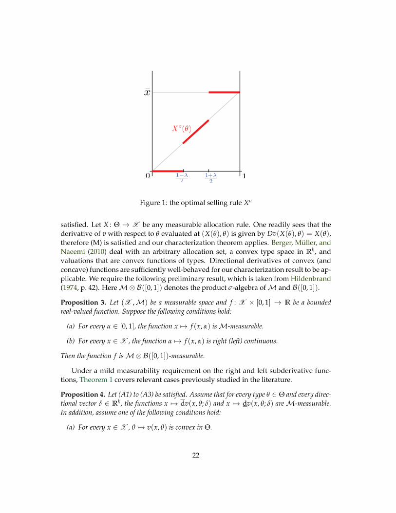
2 , and the difference in Equation 23 equals (2θ− 1− λ)(1− θ)x. Thus, the optimalselling rule is
Xo(θ) =
0, if 0 ≤ θ < 1−λ
2 ;θx, if 1−λ
2 ≤ θ < 1+λ2 ;
x, if 1+λ2 ≤ θ ≤ 1.
(24)
Notice that Xo is strictly increasing for intermediate types. Contrast this with the caseof no loss aversion (λ = 0), where the optimal selling rule gives 0 to every type θ < 1
2 ,
20
and x to every type θ ≥ 12 . The integrable selection s is therefore
s(θ) =
−λx, if 0 ≤ θ < 1−λ
2 ;(θ − λ)x, if 1−λ
2 ≤ θ < 1+λ2 ;
x, if 1+λ2 ≤ θ ≤ 1.
It is not difficult to verify that the integral monotonicity condition holds. For in-stance, for 0 ≤ θ < 1−λ
2 ≤ θ < 1+λ2 , we have v(Xo(θ), θ) − v(Xo(θ), θ) = θ(θ − θ)x,
while v(Xo(θ), θ)− v(Xo(θ), θ) = − λ(θ − θ)x, and∫ θ
θs(θ) dθ = −λ(θ − θ)x + 1
2
(θ2 −
( 1−λ2
)2)
x.
From these expression the integral monotonicity follows readily. Using Theorem 1 wededuce that Xo is implementable. The optimal selling mechanism is (Xo, po), where
po(θ) =
0, if 0 ≤ θ < 1−λ
2 ;x2
(θ2 + 2λθ + ( 1−λ
2 )2) , if 1−λ2 ≤ θ < 1+λ
2 ;x2
(λ2 + λ + 1
), if 1+λ
2 ≤ θ ≤ 1.
The reader can verify using the Mirrlees representation that the optimal sellingmechanism (Xo, po) generates an indirect utility function Uo equal to
Uo(θ) =
− λθx, if 0 ≤ θ < 1−λ
2 ;− λθx + x
2
(θ2 − ( 1−λ
2 )2) , if 1−λ2 ≤ θ < 1+λ
2 ;− λθx + x
2
(2θ(1 + λ)− λ2 − λ− 1
), if 1+λ
2 ≤ θ ≤ 1.
It is immediate to conclude that the participation constraints are satisfied. �
6 Discussion
We return to the single agent environment described in Section 2.1 to relate our tech-niques and results to recent developments in the literature.
6.1 When is (M) satisfied?
In some applications our assumption (M) is readily verified. More importantly, (M) willfollow directly from the structure of the design problem in commonly used environ-ments. Consider, as Archer and Kleinberg (2008), a setting with a bounded allocationset X ⊆ Rk, a bounded convex type space Θ ⊆ Rk, and valuation that are linear intypes, so that θ 7→ v(x, θ) = x · θ for each allocation x. Notice that (A1) to (A3) are
21
x
0 11− λ2
1+ λ2
X o(θ)
Figure 1: the optimal selling rule Xo
satisfied. Let X : Θ → X be any measurable allocation rule. One readily sees that thederivative of v with respect to θ evaluated at (X(θ), θ) is given by Dv(X(θ), θ) = X(θ),therefore (M) is satisfied and our characterization theorem applies. Berger, Muller, andNaeemi (2010) deal with an arbitrary allocation set, a convex type space in Rk, andvaluations that are convex functions of types. Directional derivatives of convex (andconcave) functions are sufficiently well-behaved for our characterization result to be ap-plicable. We require the following preliminary result, which is taken from Hildenbrand(1974, p. 42). HereM⊗B([0, 1]) denotes the product σ-algebra ofM and B([0, 1]).
Proposition 3. Let (X ,M) be a measurable space and f : X × [0, 1] → R be a boundedreal-valued function. Suppose the following conditions hold:
(a) For every α ∈ [0, 1], the function x 7→ f (x, α) isM-measurable.
(b) For every x ∈ X , the function α 7→ f (x, α) is right (left) continuous.
Then the function f isM⊗B([0, 1])-measurable.
Under a mild measurability requirement on the right and left subderivative func-tions, Theorem 1 covers relevant cases previously studied in the literature.
Proposition 4. Let (A1) to (A3) be satisfied. Assume that for every type θ ∈ Θ and every direc-tional vector δ ∈ Rk, the functions x 7→ dv(x, θ; δ) and x 7→ dv(x, θ; δ) areM-measurable.In addition, assume one of the following conditions hold:
(a) For every x ∈ X , θ 7→ v(x, θ) is convex in Θ.
22

(b) For every x ∈ X , θ 7→ v(x, θ) is concave in Θ.
(c) For every x ∈ X , θ 7→ v(x, θ) is continuously differentiable in Θ.
If X : Θ→ X is a measurable allocation rule, then (M) is satisfied.
Proof We deal with convex valuations; the remaining cases are similarly handled. Fixθ1, θ2 ∈ Θ. From (A3) and the convexity of θ 7→ v(x, θ) on Θ, it follows that for everyx ∈ X the right subderivative dv(x, θ2
1(α); δ21) is equal to the right derivative of the con-
vex real-valued function α 7→ w(α; x, δ21) = v(x, θ2
1 + α δ21) defined on (0, 1). Thus, the
function α 7→ dv(x, θ21(α); δ2
1) is right continuous on (0, 1). By assumption, the functionx 7→ dv(x, θ2
1(α); δ21) isM-measurable for every α ∈ (0, 1). Thus, we infer from Propo-
sition 3 that the function d(·, ·; δ21) isM⊗B(0, 1)-measurable. Since X is a measurable
allocation rule, it is seen that the function α 7→ (X(θ21(α)), θ2
1(α)) is B(0, 1)-measurable,hence we obtain the measurability of α 7→ s(θ2
1(α)) = dv(X(θ21(α)), θ2
1(α); δ21) by notic-
ing that the composition of measurable functions is also measurable. The argument fors(θ2
1(·)) is similar, except that in this case one uses the left derivative of the respectiveconvex scalar function, which is left continuous on (0, 1). �
Suppose that we partition X into measurable sets {X1, X2, X3}, such that for everyx ∈ X1 (respectively, X2, X3), the function θ 7→ v(x, θ) is convex in Θ (respectively,concave, continuously differentiable). One can use Proposition 4 to show that (M) isalso satisfied in this type of mixed models.
6.2 Back to Revenue Equivalence
Our revenue inequality (Theorem 2) establishes a precise range for the value of the dif-ference between two indirect utilities associated with the allocation rule X. If for alltypes θ1, θ2, the subderivative correspondence S
(θ2
1(·))
is single-valued almost every-where, then revenue equivalence is restored.
Proposition 5. Assume that (A1) to (A3) and (M) are satisfied. Let p : Θ → R and p′ : Θ →R be two payment rules that implement X : Θ → X and generate indirect utility functions Uand U′, respectively, satisfying U(θ0) = U′(θ0) = u0. If for every pair of types θ1, θ2 ∈ Θ, onehas s(θ2
1(α)) = s(θ21(α)) for almost all α ∈ (0, 1), then U = U′.
Proof Suppose that for all θ1, θ2 in Θ, it is the case that s(θ21(α)) = s(θ2
1(α)) a.e. in (0, 1).Readily from Equation 16, it follows U(θ1) = U′(θ1), for all θ1 ∈ Θ. �
We obtain the following corollary.
Corollary 2. Under the assumptions of Proposition 5, U = U′ whenever one of the followingconditions hold.
(a) For every x ∈ X , θ 7→ v(x, θ) is convex in Θ.
23
(b) For every x ∈ X , θ 7→ v(x, θ) is differentiable in Θ.
(c) The allocation set X is finite.
Proof (a) Suppose θ 7→ v(x, θ) is convex. Then, for all θ ∈ Θ and all δ ∈ Rk,
dv(x, θ; δ) = limr↑0
v(x, θ + rδ)− v(x, θ)
r≤ lim
r↓0
v(x, θ + rδ)− v(x, θ)
r= dv(x, θ; δ).
Since Equation 13 requires that at almost all equilibrium points (X(θ), θ) the reverseinequality holds, one sees that the condition of Proposition 5 is in place.
(b) Immediate.
(c) Let θ1, θ2 be arbitrary and define the function α 7→ X(α) ≡ X(θ21(α)) on (0, 1).
Since X is finite, X((0, 1)) = {x1, . . . , xN}, for some N ∈ N. Thus, the sets E1, . . . , EN ,with En = X−1({xn}) for each n = 1, . . . , N, constitute a collection of pairwise disjoint,measurable subsets of (0, 1) whose union is (0, 1). Without loss of generality, we assumethat each En has non zero measure. Then, for each n = 1, . . . , N, the function α 7→νn(α) ≡ v(xn, θ2
1(α)) is Lipschitz continuous on En and therefore differentiable a.e. inEn (by Rademacher-Stepanoff Theorem). It follows that s(θ2
1(α)) = s(θ21(α)) almost
everywhere on the unit interval (0, 1), as desired. �
Note that Corollary 2-(c) does not require the valuation function to be linear, convexor differentiable in types: for the finite allocation sets, assumptions (A1) to (A3) and (M)suffice to obtain revenue equivalence.
6.3 Weak monotonicity versus integral monotonicity
An allocation rule X : Θ → X satisfies the weak monotonicity condition if for every pairof types θ, θ in Θ, one has
v(X(θ), θ)− v(X(θ), θ) ≥ v(X(θ), θ)− v(X(θ), θ).
Weak monotonicity has been shown to characterize implementation when the typespace is convex, the valuation function linear in types, and the allocation set either finiteor infinite (the latter case requiring the inclusion of the closed-path integrability condi-tion).14 Clearly, integral monotonicity implies weak monotonicity. However, there areexamples where weak monotonicity does not imply integral monotonicity, even whenX is finite and the valuation function v(x, ·) is piecewise linear in types (Berger, Muller,and Naeemi, 2010).
On the other hand, Berger, Muller, and Naeemi (2010) discovered that a single-crossing property is sufficient to obtain the equivalence between weak monotonicity
14See Jehiel, Moldovanu, and Stacchetti (1999), Bikhchandani, Chatterji, Lavi, Mu’alem, Nisan, and Sen(2006), Saks and Yu (2005), Archer and Kleinberg (2008), and Vohra (2009).
24
and integral monotonicity, under the assumption that valuations are either convex ordifferentiable in types. As the next proposition shows, their insight extends to our gen-eral setting. Say that the valuation function v : X × Θ → R satisfies increasing differ-ences if for all x, y ∈ X , all θ1, θ2 ∈ Θ, and every θ2
1(α) ∈ L(θ1, θ2), v(x, θ2)− v(y, θ2) ≥v(x, θ2
1(α))− v(y, θ21(α)) implies that v(x, θ2
1(α))− v(y, θ21(α)) ≥ v(x, θ1)− v(y, θ1).
Proposition 6. Assume that (A1) to (A3) and (M) are satisfied for the allocation rule X : Θ→X . Suppose in addition that v : X ×Θ → R satisfies increasing differences. Then for everyθ1, θ2 in Θ, the subderivative correspondence S
(θ2
1(·))
is regular and admits an integrableselection α 7→ s(θ2
1(α)) such that X satisfies integral monotonicity if and only if X satisfiesweak monotonicity.
Proof Clearly the integral monotonicity condition implies that X is weakly monotone.Conversely, suppose that X satisfies weak monotonicity. Fix arbitrary types θ1, θ2. FromLemmas 3 and 5 of Berger, Muller, and Naeemi (2010) it follows that the increasingdifferences property of the valuation function together with weak monotonicity implythat X is cyclically monotone on the closure of L(θ1, θ2). Therefore, the restriction ofX to the closure of L(θ1, θ2) is implementable. From Theorem 1, we conclude that thesubderivative correspondence S
(θ2
1(·))
is regular and admits an integrable selectionα 7→ s(θ2
1(α)) for which integral monotonicity is satisfied. �
We stress the fact that, without additional assumptions, Proposition 6 does not im-ply that there exists a unique selection for which integral monotonicity holds. Thus,while weak monotonicity may be more readily verified in applications, we are nonethe-less interested in finding the subderivative correspondence between types and selec-tions consistent with the integral monotonicity condition, since these objects providethe (possibly many) payment rules that can be used for implementation.
7 Concluding remarks
In this paper we present a characterization of (dominant strategy) incentive compati-ble mechanisms in quasi-linear settings where the envelope theorem and the revenueequivalence principle fail, due to non-convexity and non-differentiability of the valua-tion function with respect to types. We base our characterization result on the integralmonotonicity and the Mirrlees representation of the indirect utilities (plus the standardclosed-path integrability condition). Our framework allows for the allocation set tobe finite or infinite and the type space of the agent to be a convex subset of a multi-dimensional Euclidean space. We work with uniformly Lipschitz valuations and im-pose a measurability requirement on the left and right subderivatives of the valuationfunction with respect to types.
These conditions pin down the range of payoff differences generated by two in-centive compatible mechanisms with the same allocation rule. As a consequence, we
25
obtain a revenue inequality that generalizes the standard revenue equivalence princi-ple: given an implementable allocation rule and normalized payments that assign thesame utility to the “lowest type”, the difference in equilibrium payoffs generated byany two payment rules is bounded by the allocation rule alone, even though it may benot vanish.
Our results contribute to the already extensive literature on implementation in sev-eral ways. First, our environment is less restrictive than those considered in previouswork. In particular, we do not assume linearity, convexity or differentiability of thevaluation with respect to types, but any such hypothesis, in addition to a mild measur-ability condition, will imply our assumption (M). Second, our characterization result ex-ploits techniques that differ from the approaches currently employed in the literature,thus allowing us to handle a broader set of problems with richer payment schemes.Third, our approach opens new aspects of institutional design for study. We have pro-vided two applications to illustrate this point. In particular, in certain environments itmay be possible to use several payment rules (which differ by more than just a constant)to implement an efficient or revenue maximizing allocation rule. While such schemesmay share desirable properties (e.g., budget balancedness, individual rationality), other(un)desirable features could be introduced. We leave a thorough study of these aspectsof institutional design for future research.
References
ARCHER, A., AND R. KLEINBERG (2008): “Truthful germs are contagious: a local-to-global characterization of truthfulness,” in 10th ACM Conference on Electronic Com-merce.
ASHLAGI, I., M. BRAVERMAN, A. HASSIDIM, AND D. MONDERER (2010): “Monotonic-ity and implementability,” Forthcoming: Econometrica.
AUBIN, J.-P., AND H. FRANKOWSKA (1990): Set-Valued Analysis. Birkhauser, Boston,MA.
AUMANN, R. J. (1965): “Integrals of set-valued functions,” Journal of Mathematical Anal-ysis and Applications, 12(1), 1–12.
BERGER, A., R. MULLER, AND S. H. NAEEMI (2010): “Path-monotonicity and truthfulimplementation,” Mimeo: Department of Quantitative Economics, Maastricht Uni-versity.
BIKHCHANDANI, S., S. CHATTERJI, R. LAVI, A. MU’ALEM, N. NISAN, AND A. SEN
(2006): “Weak monotonicity characterizes deterministic dominant-strategy imple-mentation,” Econometrica, 74(4), 1109–1132.
26

CARBAJAL, J. C. (2010): “On the uniqueness of Groves mechanisms and the payoffequivalence principle,” Games and Economic Behavior, 68(2), 763–772.
CHUNG, K.-S., AND W. OLSZEWSKI (2007): “A non-differentiable approach to revenueequivalence,” Theoretical Economics, 2(4), 469–487.
EISENHUTH, R. (2010): “Auction Design with Loss Averse Bidders: The Optimality ofAll Pay Mechanisms,” .
FRIEDMAN, B. (1940): “A note on convex functions,” Bulletin of the American Mathemat-ical Society, 46(6), 473–474.
GREEN, J. R., AND J.-J. LAFFONT (1979): Incentives in Public Decision-Making, Studies inPublic Economics. North-Holland, New York, NY.
HEYDENREICH, B., R. MULLER, M. UETZ, AND R. VOHRA (2009): “Characterization ofrevenue equivalence,” Econometrica, 77(1), 307–316.
HILDENBRAND, W. (1974): Core and Equilibria of a Large Economy, Princeton Studies inMathematical Economics. Princeton University Press, Princeton, NJ.
HOLMSTROM, B. (1979): “Groves’ scheme on restricted domains,” Econometrica, 47(5),1137–1144.
JEHIEL, P., B. MOLDOVANU, AND E. STACCHETTI (1996): “How (not) to sell nuclearweapons,” American Economic Review, 86(4), 814–829.
(1999): “Multidimentional mechanism design for auctions with externalities,”Journal of Economic Theory, 85(2), 258–294.
KOS, N., AND M. MESSNER (2010): “Extremal Incentive Compatible Transfers,” WorkingPapers.
KOSZEGI, B., AND M. RABIN (2006): “A model of reference-dependent preferences,”Quarterly Journal of Economics, 121(4), 1133–1165.
KRISHNA, V., AND E. MAENNER (2001): “Convex potentials with an application tomechanism design,” Econometrica, 69(4), 1113–1119.
MILGROM, P. R., AND I. SEGAL (2002): “Envelope theorems for arbitrary choice sets,”Econometrica, 70(2), 583–601.
MYERSON, R. B. (1981): “Optimal auction design,” Mathematics of Operations Research,6(1), 58–73.
RAHMAN, D. (2010): “Detecting profitable deviations,” Discussion paper, Working Pa-per, University of Minnesota.
27
ROCHET, J.-C. (1987): “A necessary and sufficient condition for rationalizability in aquasi-linear context,” Journal of Mathematical Economics, 16(2), 191–200.
ROCKAFELLAR, R. T., AND R. J.-B. WETS (1998): Variational Analysis. Springer-Verlag,Berlin.
SAKS, M., AND L. YU (2005): “Weak monotonicity suffices for truthfulness on convexdomains,” In Proceedings of the 7th ACM Conference on Electronic Commerce.
VOHRA, R. V. (2009): “Mechanism Design: a linear programming approach,” Mimeo:Kellogg Graduate School of Management, Northwestern University.
WILLIAMS, S. R. (1999): “A characterization of efficient, Bayesian incentive compatiblemechanisms,” Economic Theory, 14(1), 155–180.
28