MECHANISMS OF INSTABILITY INRAYLEIGH-BENARD CONVECTION

A ThesisPresented to

The Academic Faculty

by

Adam C. Perkins

In Partial Fulfillmentof the Requirements for the Degree

Doctor of Philosophy in theSchool of Physics

Georgia Institute of TechnologyDecember 2011

MECHANISMS OF INSTABILITY INRAYLEIGH-BENARD CONVECTION

Approved by:

Professor Michael F. Schatz, AdvisorSchool of PhysicsGeorgia Institute of Technology

Professor Alberto Fernandez-NievesSchool of PhysicsGeorgia Institute of Technology

Professor Jennifer E. CurtisSchool of PhysicsGeorgia Institute of Technology

Professor Minami YodaDepartment of MechanicalEngineeringGeorgia Institute of Technology

Professor Paul M. GoldbartSchool of PhysicsGeorgia Institute of Technology

Date Approved: 26 July 2011

To my family.

.

iii

ACKNOWLEDGEMENTS

There are many people whom I would like to acknowledge for their help and support

as I made my way through this thesis work. Mike Schatz, my advisor, deserves much

credit for the genesis of my research project. Mike’s research model of each student

being responsible for his or her experiment, the development of necessary computer

programs, data acquisition and analysis, has helped me develop many valuable skills.

Mike has always encouraged me to take advantage of speaking opportunities and has

stressed the importance of being able to discuss research with a variety of audiences.

This has proved to be invaluable advice to date, and, I expect, in the future. Mike

was also very generous with his time and helpful comments about this thesis.

Professor Roman Grigoriev provided insights on almost every occasion we spoke

about research, as well as being one of the top teachers of my graduate classes. There

were several other faculty members with whom I had many enjoyable interactions,

notably Professors Ed Conrad, Phil First, and James Gole. I would also like to thank

the committee members for suggesting ways in which to strengthen this thesis. I felt

well prepared for graduate school by the wonderful physics faculty at the University

of Northern Iowa. Professors Behroozi, Chancey, Diesz, Roth, and Shand were all

great advisors and teachers.

Many of the friends I made at Georgia Tech were helpful in getting through the

first year of classes, with Erin McGrath and Bill Knouse alternately playing the role

of social organizer. Lee Miller was a close friend as well as a roommate. Daniel

Borrero, Danny Caballero, Seungjoo Nah and Alex Wiener also became good friends

and made showing up at school each day a little more fun.

Danny and Daniel joined the Schatz lab at the same time as me; it was helpful to

iv

have others going through some of the research growing pains with me. Huseyin Kur-

tuldu, who became one of my closest friends, also worked on convection experiments

and was a great help when it came to discussing research and general experimental

issues, especially the myriad image processing obstacles that popped up.

Several people were helpful in solving various research problems. Mike Sprinkle

was kind enough to do the gold-plating of my servo mirrors on one of his clean room

trips. Matt Cornick generously provided the state estimation code and hosted me for

a visit to the University of Maryland, where he instructed me on its use. I would also

like to acknowledge Professor Werner Pesch, who, despite being retired and living in

Germany, was very quick to help when I inquired about the Busse balloon calculation.

He was very generous with his time and in providing code for the calculation.

Although unsure of what it was I was really doing, my family and friends back

home were always very supportive. Joanna Hass was wonderful, in terms of her

support and her patience. It has been both motivating and educational to work in

the research-focused environment provided by Georgia Tech, and my time living in

Atlanta has been full of memorable experiences.

v

TABLE OF CONTENTS

DEDICATION . . . . . . . . . . . . . . . . . . . . . . . . . . . . . . . . . . . iii

ACKNOWLEDGEMENTS . . . . . . . . . . . . . . . . . . . . . . . . . . . . iv

LIST OF FIGURES . . . . . . . . . . . . . . . . . . . . . . . . . . . . . . . . ix

LIST OF SYMBOLS AND ABBREVIATIONS . . . . . . . . . . . . . . . . . xv

SUMMARY . . . . . . . . . . . . . . . . . . . . . . . . . . . . . . . . . . . . . xvi

I INTRODUCTION . . . . . . . . . . . . . . . . . . . . . . . . . . . . . . 1

1.1 Pattern Formation and Instability . . . . . . . . . . . . . . . . . . 1

1.2 Rayleigh-Benard Convection . . . . . . . . . . . . . . . . . . . . . . 2

1.2.1 Introduction . . . . . . . . . . . . . . . . . . . . . . . . . . 2

1.2.2 Secondary Instability and the Busse Balloon . . . . . . . . . 6

1.2.3 Non-periodic and Time-dependent Patterns . . . . . . . . . 7

1.3 Motivation and Research Objectives . . . . . . . . . . . . . . . . . 10

1.3.1 Dynamical Systems . . . . . . . . . . . . . . . . . . . . . . . 10

II EXPERIMENTAL APPARATUS AND METHODS . . . . . . . . . . . 16

2.1 Convection Apparatus . . . . . . . . . . . . . . . . . . . . . . . . . 16

2.1.1 Optical Windows . . . . . . . . . . . . . . . . . . . . . . . . 17

2.1.2 Convection Cell . . . . . . . . . . . . . . . . . . . . . . . . . 19

2.2 Temperature and Pressure Measurement/Control . . . . . . . . . . 21

2.3 Flow Visualization . . . . . . . . . . . . . . . . . . . . . . . . . . . 24

2.3.1 Shadowgraph . . . . . . . . . . . . . . . . . . . . . . . . . . 24

2.3.2 Image Capturing . . . . . . . . . . . . . . . . . . . . . . . . 26

2.4 Infrared Light Actuation . . . . . . . . . . . . . . . . . . . . . . . . 28

2.4.1 Optics . . . . . . . . . . . . . . . . . . . . . . . . . . . . . . 31

2.5 Servo Mirror and Laser Control . . . . . . . . . . . . . . . . . . . . 33

vi

III PREPARING STRAIGHT ROLL PATTERNS . . . . . . . . . . . . . . 37

3.1 Mapping of Laser Beam to Convection Cell . . . . . . . . . . . . . 38

3.2 Straight Roll Imposition . . . . . . . . . . . . . . . . . . . . . . . . 41

3.3 Closed-loop Feedback Control . . . . . . . . . . . . . . . . . . . . . 44

3.3.1 Shadowgraph Image Analysis . . . . . . . . . . . . . . . . . 45

3.3.2 Errors . . . . . . . . . . . . . . . . . . . . . . . . . . . . . . 46

3.3.3 Control near Boundaries . . . . . . . . . . . . . . . . . . . . 50

3.3.4 Approaching Instability . . . . . . . . . . . . . . . . . . . . 50

IV PERTURBATION LIFETIMES . . . . . . . . . . . . . . . . . . . . . . 52

4.1 Experimental Procedure . . . . . . . . . . . . . . . . . . . . . . . . 53

4.1.1 Perturbation Strength . . . . . . . . . . . . . . . . . . . . . 58

4.2 Lifetime Measurements . . . . . . . . . . . . . . . . . . . . . . . . . 60

4.3 Results . . . . . . . . . . . . . . . . . . . . . . . . . . . . . . . . . 61

V MODAL EXTRACTION . . . . . . . . . . . . . . . . . . . . . . . . . . 66

5.1 Introduction . . . . . . . . . . . . . . . . . . . . . . . . . . . . . . 66

5.2 Creation of Perturbation Ensemble . . . . . . . . . . . . . . . . . . 67

5.3 Shadowgraph Image Processing . . . . . . . . . . . . . . . . . . . . 69

5.3.1 Spatial Filtering . . . . . . . . . . . . . . . . . . . . . . . . 70

5.3.2 Temporal Filtering . . . . . . . . . . . . . . . . . . . . . . . 70

5.4 Construction of Karhunen-Loeve Basis . . . . . . . . . . . . . . . . 73

5.4.1 Perturbation Averaging . . . . . . . . . . . . . . . . . . . . 75

5.5 Determination of Modal Structures and Growth Rates . . . . . . . 77

5.5.1 Use of Pattern Symmetries . . . . . . . . . . . . . . . . . . 79

5.5.2 Results . . . . . . . . . . . . . . . . . . . . . . . . . . . . . 81

5.6 Conclusions . . . . . . . . . . . . . . . . . . . . . . . . . . . . . . . 85

VI STATE ESTIMATION OF CHAOTIC PATTERNS . . . . . . . . . . . 91

6.1 Preparing Non-periodic Patterns . . . . . . . . . . . . . . . . . . . 92

6.1.1 Imposing PanAm Pattern . . . . . . . . . . . . . . . . . . . 93

vii

6.1.2 Imposing Target Pattern . . . . . . . . . . . . . . . . . . . . 96

6.1.3 Long-term Pattern Evolution . . . . . . . . . . . . . . . . . 99

6.2 Pattern Forecasting . . . . . . . . . . . . . . . . . . . . . . . . . . 102

6.2.1 Kalman Filtering . . . . . . . . . . . . . . . . . . . . . . . . 102

6.2.2 LETKF . . . . . . . . . . . . . . . . . . . . . . . . . . . . . 103

6.3 Preliminary Results . . . . . . . . . . . . . . . . . . . . . . . . . . 105

VII CONCLUSIONS . . . . . . . . . . . . . . . . . . . . . . . . . . . . . . . 111

APPENDIX A GOVERNING EQUATIONS . . . . . . . . . . . . . . . . . 115

APPENDIX B CAD DRAWINGS OF APPARATUS . . . . . . . . . . . . 119

APPENDIX C SHADOWGRAPH OPTICS . . . . . . . . . . . . . . . . . 126

APPENDIX D PROGRAM AND EXPERIMENT DETAILS . . . . . . . . 130

REFERENCES . . . . . . . . . . . . . . . . . . . . . . . . . . . . . . . . . . . 148

VITA . . . . . . . . . . . . . . . . . . . . . . . . . . . . . . . . . . . . . . . . 153

viii

LIST OF FIGURES

1.1 Rayleigh-Benard convection showing straight convection rolls. Warmfluid rises to the top of the cell, where it cools, before falling back tothe bottom. The arrows indicate the flow pattern, with bright anddark regions corresponding to warm and cool fluid, respectively. . . . 4

1.2 Stability balloons at Prandtl number 0.71 (air) and at 7.0 (water),reproduced from Ref. [1] with permission. The vertical axis is theRayleigh number and the horizontal axis is the non-dimensional wavenum-ber. The boundaries of the different types of secondary instabilities aremarked by the solid lines; the dashed lines indicate the onset of theprimary (convective) instability for the given range of wavenumbers.The area enclosed by the intersecting boundaries forms the parameterregion of stable straight roll patterns. . . . . . . . . . . . . . . . . . . 8

1.3 Snapshots of convection patterns as ε is increased. Going clockwisestarting with the image on the upper left, images are taken with ε =0.30 (a “target” pattern), ε = 0.56, ε = 0.71, ε = 0.95, ε = 1.3, and ε= 1.8. The images are taken from a convection cell with d = 608 µmand Γ = 20. . . . . . . . . . . . . . . . . . . . . . . . . . . . . . . . . 9

1.4 An image of the spatiotemporally chaotic spiral defect chaos state,taken from Ref. [2] (with permission). This experiment was with CO2

gas in a circular cell of Γ = 74.6, with ε = 0.894. . . . . . . . . . . . 11

1.5 On the left, the mid-plane temperature of a simulated SDC state.On the right is the temperature-field component of the leading Lya-punov vector; red and blue indicate large and small magnitudes, re-spectively.From Ref. [3], reproduced with permission. . . . . . . . . . 13

2.1 Schematic of the convection apparatus. . . . . . . . . . . . . . . . . . 17

2.2 On the top, unfiltered shadowgraph images capture the onset of con-vection (in a cell of depth 608 µm, Γ = 20). The Fourier power of eachshadowgraph is shown in the bottom row of images, with red corre-sponding to large power and blue to small power. From left to right, ε= -0.05, 0.02, 0.03, and 0.04 . . . . . . . . . . . . . . . . . . . . . . . 21

2.3 Schematic of closed-loop heating system for CS2 through indirect heatexchange with temperature bath. Fluid from a reservoir is drawn intoa pump, which forces the fluid through the copper coils sitting within atemperature bath, before circulating through the convection apparatusand returning to the reservoir. . . . . . . . . . . . . . . . . . . . . . . 22

ix

2.4 Temperature signals from above (top plot) and below (bottom plot)the convection cell. Both signals are under feedback control; the redlines indicate the set-point values of each: Tt = 20.0◦C and Tb = 25.0◦C. 25

2.5 Shadowgraph schematic. Rays of light are collimated and directedinto the convection cell. The light, after passing through the cell andreflecting off the bottom surface, is captured by a CCD camera. . . . 27

2.6 A shadowgraph intensity image consists of bright and dark regions thatare related to hot upflowing and cold downflowing fluid, respectively.This example shows a straight roll pattern. . . . . . . . . . . . . . . . 28

2.7 A schematic showing how the separate experimental components fitinto the overall setup: the pressurized convection cell is enclosed withinthe convection apparatus; visible light, directed from above, is usedwith the shadowgraph optics to visualize the flow; actuation usinginfrared laser light is achieved with a CO2 laser, optics to focus thelaser beam, and computer-controlled mirrors to direct the laser lightinto the convection cell from below. . . . . . . . . . . . . . . . . . . . 29

2.8 Optical system for focusing infrared laser light into convection cell.Three lenses are used to expand, collimate, and focus the light beforeit enters the cell. . . . . . . . . . . . . . . . . . . . . . . . . . . . . . 31

2.9 Voltage signal from QM2000 card. . . . . . . . . . . . . . . . . . . . . 34

2.10 Schematic showing how the voltage from the QM2000 board is used,via the UC1000 controller, to control the laser output. . . . . . . . . . 35

3.1 A schematic of the algorithm used to compute the mapping of themirror coordinates to the convection cell. . . . . . . . . . . . . . . . . 38

3.2 Shadowgraph snapshots during a mapping perturbation. The imageon the left shows the raw image containing the intensity change; theimage on the right shows the difference between the image on the leftand a background image. The images show an area of ≈ 5d× 5d. . . 40

3.3 The pattern control involves three main components, as indicated bythis schematic of the imposition/feedback algorithm. . . . . . . . . . 43

3.4 Snapshots during straight roll imposition, at approximately 3 s inter-vals. The images show the full 25 mm × 15 mm convection cell. . . . 44

3.5 Shown above is the entire convection cell (and part of the cell bound-aries, where the rolls terminate), showing the straight roll pattern un-der control (the curved rolls at the top are outside the region of con-trol). Underneath the roll pattern is a profile of intensity values acrossthe image, in the direction of the wavevector, as indicated by the lineoverlayed on the pattern. . . . . . . . . . . . . . . . . . . . . . . . . . 47

x

3.6 Local quadratic fits to the intensity maxima/minima. The intensityvalues are given by the circles in blue; the fits are shown in red. . . . 48

4.1 The Busse balloon showing various instabilities (CR, cross roll; ECK,Eckhaus; SV, skew-varicose; OSC, oscillatory) of the straight roll state,at a Prandtl number of 0.84, as in our experiments. The high-wavenumberregion under study has been highlighted. . . . . . . . . . . . . . . . . 54

4.2 An image showing the straight roll pattern under control. . . . . . . . 55

4.3 The local wavenumber field computed for the straight roll pattern inFig. 4.2. The dashed lines indicate the approximate locations of up-flowing fluid. The colormap scale has been chosen to match that ofFig. 4.6. . . . . . . . . . . . . . . . . . . . . . . . . . . . . . . . . . . 56

4.4 The probability distribution of local wavenumbers, as measured fromthe pattern in Fig. 4.2. . . . . . . . . . . . . . . . . . . . . . . . . . . 57

4.5 A pattern shortly after a point perturbation to the center cold roll(dark regions are cold down-flow; bright regions are warm up-flow). . 58

4.6 A local wavenumber field immediately following a perturbation. As inFig. 4.3, dashed lines indicate the approximate locations of upflowingfluid in the base state. . . . . . . . . . . . . . . . . . . . . . . . . . . 59

4.7 The local separation of adjacent upflow regions over time, after a per-turbation to the cold downflow region in between. The red line showsan exponential fit. . . . . . . . . . . . . . . . . . . . . . . . . . . . . . 62

4.8 Decay rates (i.e., inverses of lifetimes) over a range of pattern wavenum-bers. The error bars represent the 10% uncertainty in any one lifetimemeasurement. . . . . . . . . . . . . . . . . . . . . . . . . . . . . . . . 63

5.1 The Busse balloon for Prandtl number 0.84 as in our experiments. Theparameter coordinates of the three separate experimental ensembles areindicated by DI , DII and DIII . DI = (0.60, 2.85), DII = (1.50, 2.40),and DIII = (0.60, 2.20). Also marked is the wavenumber range aroundDI over which perturbation lifetimes were measured (see Chapter 4). 68

5.2 Perturbations are applied at different points along the direction of thepattern wavenumber (indicated by the arrow); perturbations across ahalf-wavelength constitute a minimal set. . . . . . . . . . . . . . . . . 69

5.3 Images showing how the structures excited by perturbations can be vi-sualized by subtracting off the stationary straight roll pattern. On thetop are the raw images immediately following a perturbation and thenat a short time (about 1 s) later. On the bottom are the same imagesafter the straight rolls (with no perturbation) have been subtracted. . 71

xi

5.4 Snapshots (at DI , with q = 2.85) show the decay of the excited struc-tures after an initial perturbation. This example is the result of aperturbation to a region of cold downflow and shows the structure atregularly spaced intervals over 2.5 seconds. The area shown covers oversix wavelengths of the base straight roll pattern. . . . . . . . . . . . . 72

5.5 The fraction of the total variance accounted for by the KL basis modesat DI as a function of the basis size. . . . . . . . . . . . . . . . . . . 76

5.6 The fraction of the total variance accounted for by the KL basis modesat DI as a function of the basis size, after averaging perturbations ateach respective location. . . . . . . . . . . . . . . . . . . . . . . . . . 77

5.7 The KL basis images at DI . As in Fig. 5.4, the area shown covers oversix wavelengths of the base straight roll pattern. . . . . . . . . . . . . 78

5.8 Two symmetry planes are defined over a half-wavelength of the pattern,one at the center of (hot) upflowing fluid, the other at the center ofadjacent (cold) downflowing fluid. Four symmetric versions of eachdisturbance are formed by decomposing the disturbance into even/oddstructures about either symmetry plane. . . . . . . . . . . . . . . . . 80

5.9 The four symmetric modes extracted at DI . The top two images showthe pair of structures sharing the largest growth rate; the two sub-dominant modes are shown below. Dashed lines mark the approximatelocations of the hot upflow of the underlying base state; cold fluid liesbetween the dashed lines. (The distance between adjacent dashed linesis one pattern wavelength.) . . . . . . . . . . . . . . . . . . . . . . . . 83

5.10 On the left, versions of the dominant (top) and sub-dominant (bot-tom) modes extracted at DI . Next to these for comparison are modesextracted from the second high-wavenumber ensemble at DII . The im-ages have been scaled to show the patterns, over six wavelengths, usingthe same image size. . . . . . . . . . . . . . . . . . . . . . . . . . . . 84

5.11 The four symmetric modes extracted at DIII . As in Fig. 5.9, thetop two images show the modal structures sharing the largest growthrate, and the two sub-dominant modes are shown below. Again, thedashed lines show the approximate locations of hot upflow; the distancebetween adjacent dashed lines is one pattern wavelength. . . . . . . . 86

5.12 The set of possible representations of the dominant mode extracted atDI . The most spatially localized (fundamental) mode is constructedfrom a linear combination of these modes. . . . . . . . . . . . . . . . 87

5.13 Fundamental representations of (a) the dominant and (b) sub-dominantmode high-wavenumber modes extracted at DI . . . . . . . . . . . . . 87

xii

5.14 Fundamental representations of (a) the dominant and (b) sub-dominantmode high-wavenumber modes extracted at DIII . . . . . . . . . . . . 88

5.15 Examples of using the most spatially localized version of a mode to fita more-extended version. On the left are the more-extended symmetricmodes extracted, and on the right are the best fits using only translatedcopies of the corresponding spatially localized mode. From top tobottom, the modes are the dominant mode at DI followed by the sub-dominant mode at DI and then the dominant mode at DIII. . . . . 89

6.1 An axisymmetric target pattern is observed in our convection cell nearonset (cell aspect ratio Γ = 20, and ε = 0.10). . . . . . . . . . . . . . 93

6.2 An example of a stationary PanAm pattern in a small aspect ratio(Γ = 7.66) cylindrical cell of argon gas, ε = 0.05. Reproduced fromRef. [4], with permission. . . . . . . . . . . . . . . . . . . . . . . . . . 94

6.3 Snapshots showing the imposition of a panam pattern (in time, fromleft to right and top to bottom). Here, and in all other circular con-vection patterns in this chapter, Γ = 20 (except where noted). . . . . 95

6.4 Snapshots showing the imposition of a target pattern. . . . . . . . . . 97

6.5 Shadowgraphs showing the evolution of two patterns from nearly iden-tical imposed patterns. The images span over two minutes. . . . . . . 98

6.6 Shadowgraphs showing the evolution of two patterns from nearly iden-tical imposed patterns, continued in Fig. 6.7. . . . . . . . . . . . . . . 100

6.7 The continued evolution of the patterns in Fig. 6.6. The images weretaken over the course of three minutes. . . . . . . . . . . . . . . . . . 101

6.8 Snapshots at ε = 0.60, showing sustained time-dependent patterns.Relative to the pattern on the left, the center pattern is taken after4th; the pattern at the right is taken after 30th. . . . . . . . . . . . . 102

6.9 On top, the average Rayleigh number of the ensemble, as shadowgraphsare assimilated; below, the standard deviation in the ensemble Rayleighnumbers, relative to the average Rayleigh number at that time. . . . 106

6.10 On top, the average value of the shadowgraph parameter a over theensemble, as shadowgraphs are assimilated; below, the standard devi-ation in the ensemble a values, relative to the average value at thattime. . . . . . . . . . . . . . . . . . . . . . . . . . . . . . . . . . . . . 107

6.11 The root mean square error between the predicted and observed shad-owgraph over assimilation (arbitrary units). . . . . . . . . . . . . . . 108

xiii

6.12 On the left are the actual shadowgraphs; on the right are those com-puted from the model state. These three images are taken at 30tv,50tv, and 56tv (from top to bottom). . . . . . . . . . . . . . . . . . . 109

B.1 The top cell plate, part I. . . . . . . . . . . . . . . . . . . . . . . . . 120

B.2 The top cell plate, part II. . . . . . . . . . . . . . . . . . . . . . . . . 121

B.3 The bottom cell plate, part I. . . . . . . . . . . . . . . . . . . . . . . 122

B.4 The bottom cell plate, part II. . . . . . . . . . . . . . . . . . . . . . . 123

B.5 The cooling (heating) chamber. . . . . . . . . . . . . . . . . . . . . . 124

B.6 The small plate used to hold the outer windows of the apparatus. . . 125

xiv

LIST OF SYMBOLS AND ABBREVIATIONS

Symbol or Abbreviation Description

RBC Rayleigh-Benard convection

Ra Rayleigh number

Rac critical Ra (onset of convection)

Pr Prandtl number

d depth of convection cell

Γ cell aspect ratio

∆T temperature difference across cell

∆Tc critical ∆T (onset of convection)

ε reduced Rayleigh number,Ra−RacRac

q straight roll pattern wavenumber

qc critical q (onset of instability)

SDC spiral defect chaos

LETKF Local Ensemble Transform Kalman Filter

tv, th vertical, horizontal diffusion time

CR cross roll

ECK Eckhaus

SV skew-varicose

OSC oscillatory

τ perturbation lifetime

LS Lasershow Designer 2000 software

xv

SUMMARY

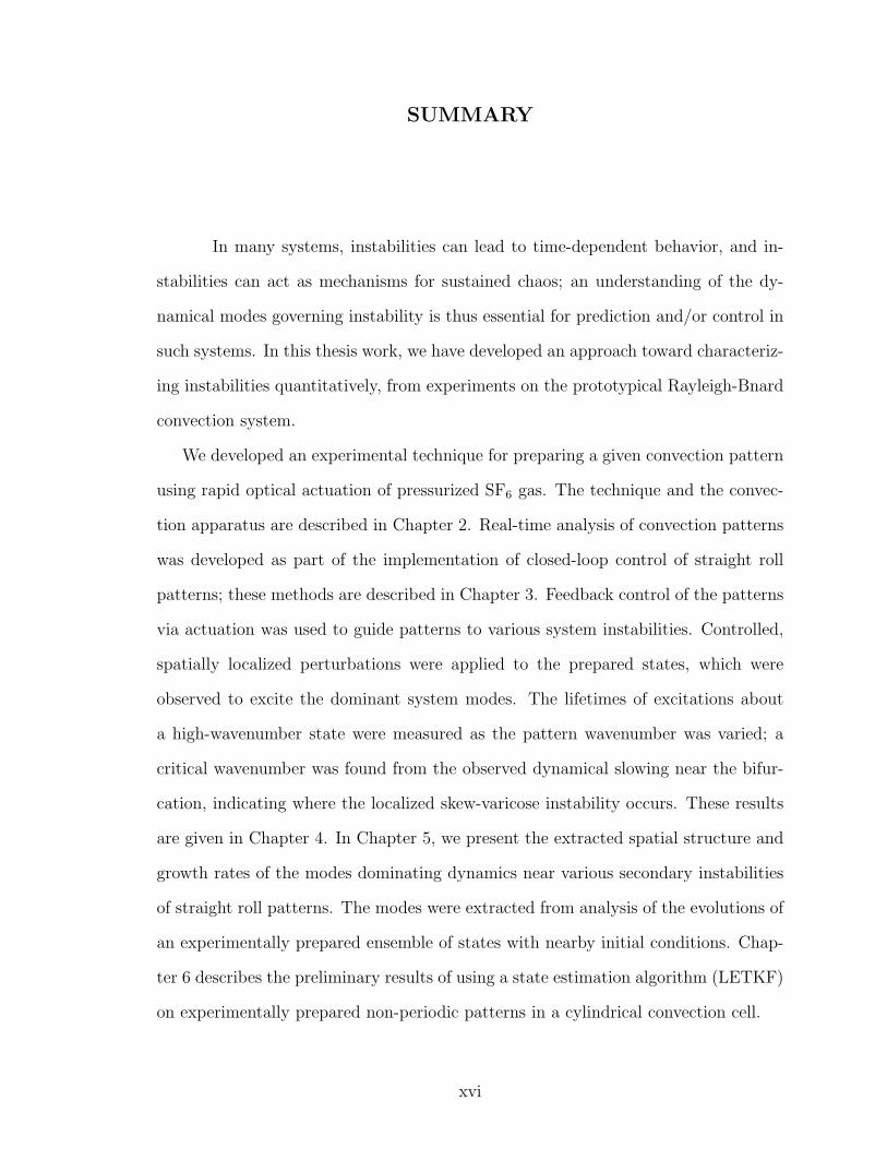
In many systems, instabilities can lead to time-dependent behavior, and in-

stabilities can act as mechanisms for sustained chaos; an understanding of the dy-

namical modes governing instability is thus essential for prediction and/or control in

such systems. In this thesis work, we have developed an approach toward characteriz-

ing instabilities quantitatively, from experiments on the prototypical Rayleigh-Bnard

convection system.

We developed an experimental technique for preparing a given convection pattern

using rapid optical actuation of pressurized SF6 gas. The technique and the convec-

tion apparatus are described in Chapter 2. Real-time analysis of convection patterns

was developed as part of the implementation of closed-loop control of straight roll

patterns; these methods are described in Chapter 3. Feedback control of the patterns

via actuation was used to guide patterns to various system instabilities. Controlled,

spatially localized perturbations were applied to the prepared states, which were

observed to excite the dominant system modes. The lifetimes of excitations about

a high-wavenumber state were measured as the pattern wavenumber was varied; a

critical wavenumber was found from the observed dynamical slowing near the bifur-

cation, indicating where the localized skew-varicose instability occurs. These results

are given in Chapter 4. In Chapter 5, we present the extracted spatial structure and

growth rates of the modes dominating dynamics near various secondary instabilities

of straight roll patterns. The modes were extracted from analysis of the evolutions of

an experimentally prepared ensemble of states with nearby initial conditions. Chap-

ter 6 describes the preliminary results of using a state estimation algorithm (LETKF)

on experimentally prepared non-periodic patterns in a cylindrical convection cell.

xvi

CHAPTER I

INTRODUCTION

1.1 Pattern Formation and Instability

Pattern-forming systems are ubiquitous. Astrophysical patterns can be seen on the

surfaces of the Sun and planets (sun-spots, stripes on Jupiter, etc.). Patterns are

observed in chemical systems (e.g., reaction-diffusion systems). Some of the most

striking and most complex pattern-forming systems are biological, including the vis-

ible structures of plants and animals as well as internal systems such as organs and

neuronal networks.

These are all examples of systems maintained out of equilibrium, systems in which

dissipative mechanisms compete against a flow of energy into the system. Despite

important physical differences, it turns out that many features observed across a

variety of systems share a common mathematical description [5, 6]. It is hoped

that the study of these shared features will help to build a general approach to

characterizing and understanding non-equilibrium systems, rather than be left with

treating systems on a case by case basis [7].

Generally speaking, a spatially extended, uniform state gives rise to a spatial

pattern (with or without time dependence) as a result of instability. This so-called

primary instability occurs when one or more system ‘control’ parameters exceed crit-

ical values. Control parameters can be thought of as the “knobs” accessible to the

experimenter (or theorist); they can be adjusted systematically through some change

in experimental conditions, for example. In many systems, the control parameter is

related to the relative rates at which energy or some other relevant quantity (e.g., the

1

concentration of some chemical) is added to or dissipated from the system. At val-

ues different from critical, these control parameters can be used to define a distance

above or below the onset of primary instability1. The particular pattern that emerges

will depend on the governing equations (in addition to stochastic processes, such as

thermal fluctuations) but, in many cases, a stationary pattern emerges with relatively

simple spatial dependence (e.g., a small number of Fourier modes). However, as the

distance above onset is increased, this primary pattern may itself undergo a transi-

tion to another state as a result of secondary instability. In principle, tertiary and

higher instabilities could result in a succession of different time-independent patterns

as the distance from onset is increased. In practice, instabilities often lead to com-

plex (chaotic), time-dependent states where a quantitative understanding of pattern

dynamics is limited.

1.2 Rayleigh-Benard Convection

1.2.1 Introduction

Rayleigh-Benard convection (many times hereafter referred to as RBC) has long been

an experimental and theoretical paradigm of pattern-forming systems (“the grand-

daddy of canonical examples” [8]). Its study is useful for understanding common

aspects of pattern formation such as pattern competition, saturation, and the effects

of physical boundaries. Additionally, RBC displays rich dynamics, ranging from sta-

tionary patterns to weakly chaotic evolution to highly turbulent states; the dynamical

regime can be tuned by a small number of parameters. Moreover, convection is an im-

portant part of many physical systems and processes such as the weather, the Earth’s

mantle, solar flares, and oceanic currents, to name just a few examples. For these

1For clarity, consider as an example a system with a single control parameter: a pattern emergeswhen the control parameter exceeds (is ‘above’) a critical value; when the parameter is smaller than(‘below’) the critical value, there is no pattern. In systems with multiple control parameters, thequantitative meaning of ‘distance above’ and ‘distance below’ can be more ambiguous, but may stillbe used qualitatively to imply whether or not the system has undergone the instability of interest.

2

reasons, RBC is an excellent system on which to test new ideas and approaches for

understanding nonlinear dynamics.

In its most basic description, RBC consists of a thin layer of fluid extending in the

plane normal to the direction of gravitational acceleration (for many purposes, the

lateral extent can be taken to be infinite); the fluid is heated from below and cooled

from above. The temperature difference (∆T ) across the fluid gives rise to density

differences, as regions of fluid near the bottom (top) boundary are warmed (cooled)

and hence expand (contract). The density differences in turn result in a buoyancy

force, which acts to reorganize the lighter fluid at the top boundary (and heavier

fluid at the bottom). For small ∆T , the fluid remains motionless; heat is transferred

across the fluid through conduction, with a linear temperature profile across the fluid

layer. When the temperature difference exceeds some critical value (∆Tc), energy

transfer through reorganization of hot/cold fluid becomes more efficient than thermal

and viscous dissipation and fluid motion sets in. Benard in 1900-1901 [9, 10] was the

first to report careful experiments on the convective motion in a fluid heated from

below, and Rayleigh provided a theoretical explanation of the buoyancy-driven motion

in 1916 [11]. It turns out that surface tension was partly responsible for Benard’s

observed fluid motion, a phenomenon now known as Benard-Marangoni convection,

but the work by Rayleigh was nonetheless very important in that it provided an

accurate description of the mechanism of primary instability and the proper non-

dimensional combination of fluid and other system properties forming the relevant

control parameter. This parameter is now known as the Rayleigh number. Rayleigh

treated the problem of a fluid with free boundaries; Jeffreys extended this approach

to the more physical, but more challenging, case of rigid boundaries [12, 13].

The set of equations governing the evolution of the convecting fluid are known as

the Boussinesq equations [14, 15]. The Boussinesq equations are derived from the full

Navier-Stokes under the assumption that the temperature dependence of the fluid

3

Figure 1.1: Rayleigh-Benard convection showing straight convection rolls. Warm fluidrises to the top of the cell, where it cools, before falling back to the bottom. Thearrows indicate the flow pattern, with bright and dark regions corresponding to warmand cool fluid, respectively.

properties can be neglected, except in the case of the density, which is assumed to

have a linear temperature dependence. A derivation of the Boussinesq equations is

given in Appendix A; the reader is referred to Ref. [16] for a more detailed treatment2.

The non-dimensional Boussinesq equations read:

∇ ·V = 0 (1.1)

Pr−1(∂V

∂t+ (V · ∇)V) = −∇P +∇2V + θz (1.2)

∂θ

∂t+ (V · ∇)θ = ∇2θ +RaVz (1.3)

Here, V and θ are the velocity and the deviation of the temperature from the linear

conduction profile, respectively. In addition to these two fields that describe the fluid

state (and the pressure P ), a pair of non-dimensional parameters (Ra and Pr) are

2For a discussion of non-Boussinesq effects on pattern formation and evolution, see Ref. [17] andthe references therein or, more recently, Refs. [18, 19].

4

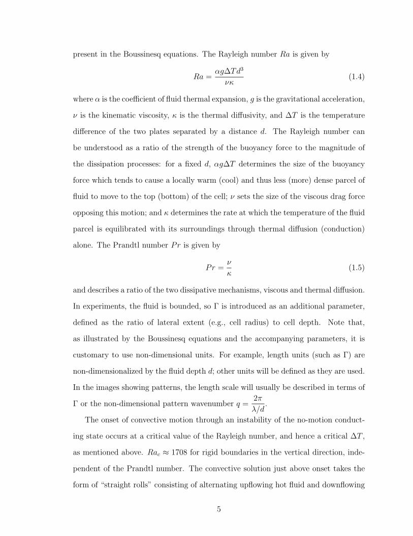
present in the Boussinesq equations. The Rayleigh number Ra is given by

Ra =αg∆Td3

νκ(1.4)

where α is the coefficient of fluid thermal expansion, g is the gravitational acceleration,

ν is the kinematic viscosity, κ is the thermal diffusivity, and ∆T is the temperature

difference of the two plates separated by a distance d. The Rayleigh number can

be understood as a ratio of the strength of the buoyancy force to the magnitude of

the dissipation processes: for a fixed d, αg∆T determines the size of the buoyancy

force which tends to cause a locally warm (cool) and thus less (more) dense parcel of

fluid to move to the top (bottom) of the cell; ν sets the size of the viscous drag force

opposing this motion; and κ determines the rate at which the temperature of the fluid

parcel is equilibrated with its surroundings through thermal diffusion (conduction)

alone. The Prandtl number Pr is given by

Pr =ν

κ(1.5)

and describes a ratio of the two dissipative mechanisms, viscous and thermal diffusion.

In experiments, the fluid is bounded, so Γ is introduced as an additional parameter,

defined as the ratio of lateral extent (e.g., cell radius) to cell depth. Note that,

as illustrated by the Boussinesq equations and the accompanying parameters, it is

customary to use non-dimensional units. For example, length units (such as Γ) are

non-dimensionalized by the fluid depth d; other units will be defined as they are used.

In the images showing patterns, the length scale will usually be described in terms of

Γ or the non-dimensional pattern wavenumber q =2π

λ/d.

The onset of convective motion through an instability of the no-motion conduct-

ing state occurs at a critical value of the Rayleigh number, and hence a critical ∆T ,

as mentioned above. Rac ≈ 1708 for rigid boundaries in the vertical direction, inde-

pendent of the Prandtl number. The convective solution just above onset takes the

form of “straight rolls” consisting of alternating upflowing hot fluid and downflowing

5

cold fluid (see Fig. 1.1) with a single spatial frequency in one of the lateral directions.

The non-dimensional wavenumber of this critical Fourier mode is also independent

of Prandtl number3 and is given by qc = 3.117 [16]. In experiments, the convection

pattern at onset will generally deviate somewhat from ideal; for example, strongly

bounded systems will likely have a wavenumber different from qc, and in cylindrical

geometry, the convection pattern can take the form of a target pattern, as shown in

Fig. 1.3 (and later in Fig. 2.2). At Rayleigh numbers above critical, it is convenient to

use a parameter known as the reduced Rayleigh number, ε ≡ Ra−Rc

Rc

(which simpli-

fies to ε =∆T

∆Tc− 1 under the Boussinesq approximation), to indicate the distance

from onset. Pattern visualization is achieved via the shadowgraph method, which

transforms the three-dimensional flow pattern into a two-dimensional intensity image

showing regions of hot/cold fluid across the cell’s lateral domain. The shadowgraph

method is described in detail in Section 2.3.

1.2.2 Secondary Instability and the Busse Balloon

For ε > 0, a range of possible pattern wavenumbers emerge, only some of which

are observed experimentally. Starting in the 1960s, Busse and coworkers used the

Boussinesq equations to construct a theoretical description of the different straight

roll patterns arising near the primary convective instability [20, 21, 22]. This seminal

work examined secondary instabilities, wherein the straight roll state loses stability.

These instabilities cause the joining of existing hot upflow (cold downflow) regions

or the introduction of new convection rolls, the overall result being a reorganization

of the straight roll state. Effectively, these secondary instabilities limit the range

of parameter values (the relevant parameters are the Rayleigh and Prandtl numbers

as well as the pattern wavenumber) for which the straight roll pattern is predicted

to be stable and can thus be expected to be observed in experiments; this volume

3The Prandtl number appears as a coefficient on a nonlinear term in the Boussinesq equationsand is thus neglected when investigating the linear stability of the conducting state.

6

of parameter space is bounded by what has been labeled eponymously the Busse (or

stability) balloon. Which of the various instabilities form the balloon boundaries, and

at what values those instabilities occur, is largely dependent on the Prandtl number.

For this reason, the stability balloon is shown typically with fixed Pr, producing two-

dimensional slices in (q, Ra) space. Figure 1.2 shows the Busse balloons at Pr = 7

(water) and Pr = 0.71 (air), from which one notices substantial differences both in

the limiting instability types and where in the space they occur. See Refs. [21, 22, 23]

for a detailed description of the various types of secondary instabilities.

1.2.3 Non-periodic and Time-dependent Patterns

Above the onset of convection, (ε > 0), the selection of the pattern that emerges and

its spatiotemporal character are influenced heavily by the fluid’s Prandtl number.

This can be understood intuitively by noting the appearance of the Prandtl number

in the evolution equation for the fluid velocity; small Prandtl numbers effectively

enhance the strength of the non-linearity in this equation. The result for small-Pr

fluids (Pr ≈ 1 for typical gases) is the likely development of a flow pattern in the

lateral directions (known as a mean flow) that couples positively with roll curva-

ture [24, 25, 26]. This is in contrast to periodic straight rolls, which have no overall

flow pattern in the horizontal directions and no roll curvature. Because convection

rolls have a tendency to terminate at right angles to the convection cell boundaries

(sidewalls)4, boundaries can become local sources of roll curvature, coupling back

to the mean flow. The result is that ideal straight roll patterns are unlikely to be

observed except very near onset.

Figure 1.3 shows shadowgraph snapshots during a progression of patterns at in-

creasing values of ε. The shadowgraph method is described in Section 2.3; roughly

4The velocity must be zero at the cell boundaries (no-slip); aligning a given roll at a right angle toa boundary is a way of meeting that condition with little effect on the roll flow pattern (as opposedto aligning the convection roll parallel to the boundary).

7

Figure 1.2: Stability balloons at Prandtl number 0.71 (air) and at 7.0 (water), re-produced from Ref. [1] with permission. The vertical axis is the Rayleigh numberand the horizontal axis is the non-dimensional wavenumber. The boundaries of thedifferent types of secondary instabilities are marked by the solid lines; the dashedlines indicate the onset of the primary (convective) instability for the given range ofwavenumbers. The area enclosed by the intersecting boundaries forms the parameterregion of stable straight roll patterns.

8

Figure 1.3: Snapshots of convection patterns as ε is increased. Going clockwisestarting with the image on the upper left, images are taken with ε = 0.30 (a “target”pattern), ε = 0.56, ε = 0.71, ε = 0.95, ε = 1.3, and ε = 1.8. The images are takenfrom a convection cell with d = 608 µm and Γ = 20.

speaking, bright (dark) areas on the image correspond to hot (cold) fluid. On the

upper left is an example of a “target” pattern, the analog of straight rolls in a circu-

lar convection cell. This imprinting of the cell geometry onto the convection pattern

is an example of what is known as sidewall forcing, which is most often due to a

mismatch in the thermal conductivities between the boundary and the convective

fluid. In this set of images, ε has been increased rapidly, causing remnants of the

initial circular symmetry to be present transiently, even at moderate ε. Eventually,

the pattern evolves to align the rolls at right angles to the sidewalls, and the spatial

complexity of the pattern increases with increasing ε. Point-like regions of fluid, like

those present in the final image, are referred to as defects, and they play an important

role in pattern evolution.

For sufficiently large aspect ratio convection cells, there exists a spatiotemporally

9

chaotic state known as the spiral defect chaos (SDC) state [2], a state characterized

by rotating spirals and regions of locally parallel rolls, punctuated by defects; see

Fig. 1.4. Intriguingly, it as been shown experimentally that the SDC state is bistable

with the straight roll pattern [27] over a certain parameter range. That is, for certain

parameter values, one can observe either a stationary, spatially periodic state, or a

state exhibiting chaos in both space and time; because the physical sidewalls can be

sources of roll curvature or defects, it is suspected that their presence tends to predis-

pose the system toward SDC (i.e., the sidewalls put the system into the SDC basin

of attraction) [28], meaning straight roll patterns are usually observed only under

special experimental conditions (e.g., using sidewalls with non-uniform conductivity).

1.3 Motivation and Research Objectives

Chaotic convection states, like SDC, are particularly interesting because they allow

one to study different ideas about chaotic evolution in an experimental system where

conditions are well controlled, the evolution equations are known, and high-resolution

measurements can be made. Several studies have attempted to characterize SDC

through statistical measures, such as the number of defects or spirals [29] or through

the Fourier power spectrum and correlation lengths/times [28]. What dynamical role

these measures play, however, is unclear.

1.3.1 Dynamical Systems

The approach of dynamical systems theory is to picture a system state within a

space spanned by the dynamical variables [7]; this space is termed the dynamical

phase space. The phase space for RBC, in principle, consists of velocity vectors

and temperature scalar values at every fluid particle position. System evolution is

then visualized by a trajectory through points in the phase space. (Perhaps the best

known example is the butterfly-like appearance of trajectories around the Lorenz

attractor [30].) For simple patterns, or in certain representations, the dimensionality

10

Figure 1.4: An image of the spatiotemporally chaotic spiral defect chaos state, takenfrom Ref. [2] (with permission). This experiment was with CO2 gas in a circular cellof Γ = 74.6, with ε = 0.894.

11

of the space may reduce substantially, as is the case with the ideal straight roll state

and the corresponding three-dimensional space embedding the Busse balloon. It is

not known, however, for a general chaotic state, the degree to which the number of

dimensions can be reduced while still capturing the full state evolution.

The different ways in which patterns can evolve from a given state are known as

the dynamical modes (or local Lyapunov vectors); it is the number of these modes

needed to capture an evolution that determines the dimension of a state, and it is

the structure of these modes that describe the actual changes to a pattern. Together

with each dynamical mode is a growth rate that indicates the rate at which small

disturbances to the given state, in the form of the respective mode, can be expected to

grow (positive growth rate) or decay (negative growth rate); it is therefore the modes

with the largest growth rates that are likely to be responsible for pattern evolution.

Computational advances have recently allowed for the direct numerical computa-

tion of the dynamical modes of the SDC state [3]. Shown in Fig. 1.5 are the mid-plane

temperature field and the corresponding temperature-component of the leading mode

(Lyapunov vector) from a snapshot of a simulated spiral defect chaos state. Notice-

able in the Lyapunov field is a high degree of spatial localization (i.e., most of the

vector’s magnitude is contained in a small area of space), indicating that the mecha-

nism responsible for separating trajectories acts on a spatially localized scale through

the creation/annihilation of defects occurring in straight roll regions of the pattern.

In fact, the instabilities that were observed to contribute to chaotic evolution are

instabilities of the straight roll pattern itself.

While the Busse balloon addresses the question of straight roll stability in the

case of (infinite) ideal rolls, such patterns are rarely observed experimentally. More

often is the case where a straight roll pattern is not strictly periodic: the presence of

physical boundaries can be accommodated by an integer number of rolls with non-

uniform spacing or can result in more than one pattern wavevector (so that rolls can

12

Figure 1.5: On the left, the mid-plane temperature of a simulated SDC state. Onthe right is the temperature-field component of the leading Lyapunov vector; red andblue indicate large and small magnitudes, respectively.From Ref. [3], reproduced withpermission.

more closely meet all boundaries at right angles). The positive feedback between roll

curvature and mean flow in low-Pr fluids makes areas of these non-ideal patterns

with locally higher or lower roll spacing most susceptible to pattern instabilities. The

upshot is that instabilities in experimental straight roll patterns tend to occur in

spatially localized, rather than global, regions, just as in SDC. While these straight

roll instabilities can result simply in a change in pattern wavenumber or orientation,

they can also introduce defects into the pattern that can cause further roll distortions

and thus lead to a growing cascade of instabilities. The result of such a defect cascade

can be a transition from stationary straight rolls to a time-evolving (chaotic) pattern

such as SDC.

To date, there exists no general experimental approach to obtaining the dominant

dynamical modes of nonlinear non-equilibrium systems; such an approach could be

useful in systems where the governing equations are unknown or the system geome-

try does not lend itself easily to numerical modeling. The research presented in this

thesis has been motivated by a desire to characterize experimentally the mechanisms

of instability of the straight roll pattern; because these instabilities remain relevant

13

dynamically in more complex states (e.g., SDC), this work is a step toward character-

izing complex (chaotic) pattern evolution directly from experimental measurements.

That spatially localized instabilities continue to be important in the chaotic evolution

of patterns suggests that it is through these types of instability events that patterns

with nearby initial conditions diverge. It is natural, therefore, to expect that these

events also play a role in limiting predictive capabilities. In this thesis, we present

preliminary work aimed at applying a particular prediction algorithm to patterns

which have been prepared with controlled initial conditions, as they evolve via roll

instabilities. Many of the different techniques for extracting, analyzing, and char-

acterizing the experimental data presented herein are developed generally, with the

idea in mind that much of our approach can be carried over to other non-equilibrium

systems, where understanding of the important system modes may prove useful for

control and/or prediction of system dynamics.

14

.

15

CHAPTER II

EXPERIMENTAL APPARATUS AND METHODS

As discussed in the Introduction, the rich behavior observed in convection studies

of low Prandtl number fluids (Pr ≈ 1 for a typical gas) makes gas convection of

particular interest. However, high quality pattern imaging (see shadowgraph discus-

sion below) of gases at atmospheric pressures is difficult due to their low density.

For this reason, it is common to conduct convection experiments with pressurized

gases [31, 32, 17]. This chapter provides an overview of the pressurized convection

apparatus and other essential experimental components used in this thesis work. It

has been written with the intent to focus on the novel features; accordingly, much

of this chapter is devoted to describing in detail the components and techniques for

actuation of the fluid flow using infrared laser light. The ability provided by this ex-

perimental tool, of manipulating convective patterns in a controlled fashion, is central

to this thesis work. It is only appropriate to also give an explanation of shadowgraph

visualization of the convection patterns, which account for the entirety of the ex-

perimental data. The experimental procedures are discussed in subsequent chapters,

where appropriate. Further details regarding the design, maintenance, and operation

of the experiment can be found in Appendix D.

2.1 Convection Apparatus

The design of our experimental apparatus is based on the description given by de

Bruyn et al. [32] for shadowgraph visualization of compressed gas convection. A

schematic is shown in Fig. 2.1. The convection cell is formed between two pressure

windows which transmit visible light, allowing for flow visualization. The fluid, com-

pressed sulfur hexafluoride (SF6) is bounded laterally by a set of sidewalls; together,

16

ConvectionCell

Sapphire Window

ZnSe Window

Water

CS2

Glass Window

ZnSe Window

Sidewalls

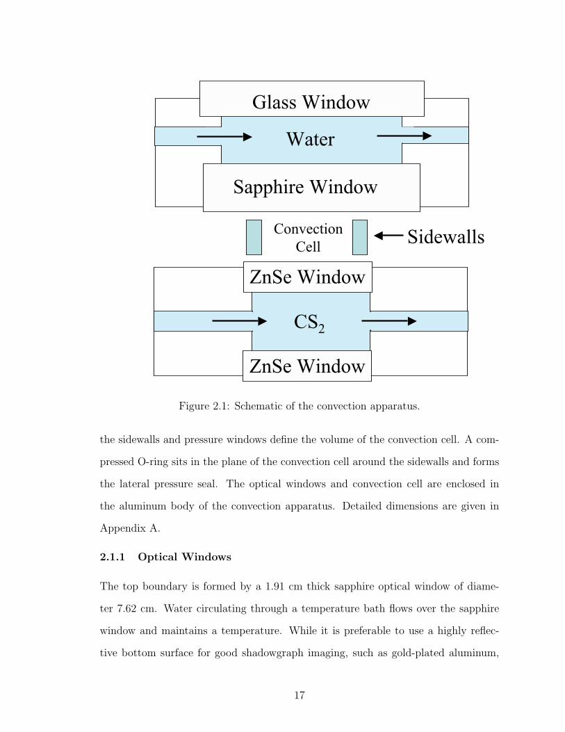
Figure 2.1: Schematic of the convection apparatus.

the sidewalls and pressure windows define the volume of the convection cell. A com-

pressed O-ring sits in the plane of the convection cell around the sidewalls and forms

the lateral pressure seal. The optical windows and convection cell are enclosed in

the aluminum body of the convection apparatus. Detailed dimensions are given in

Appendix A.

2.1.1 Optical Windows

The top boundary is formed by a 1.91 cm thick sapphire optical window of diame-

ter 7.62 cm. Water circulating through a temperature bath flows over the sapphire

window and maintains a temperature. While it is preferable to use a highly reflec-

tive bottom surface for good shadowgraph imaging, such as gold-plated aluminum,

17

our desire to direct infrared light from below (as described in Section 2.4) limits the

choice of material. We use a 0.95 cm thick zinc selenide (ZnSe) optical window of

diameter 5.08 cm and control the window temperature via circulating carbon disulfide

(CS2). Both ZnSe and CS2 have high transmission at the wavelength (10.6 µm) of

the infrared laser light used in the experiments.

Pressure Loading Thick optical windows are needed to withstand the large

gas pressures; a typical experiment is conducted near 200 psi. While zinc selenide is a

material commonly used in CO2 laser applications, thick material is difficult to find.

The minimum thickness of the material for a given pressure load and desired radius

is given by the following expression1:

Tmin =

√1.1PR2S

M(2.1)

where T is the material thickness, M is the material rupture modulus, P is the

pressure differential across the window, R is the radius of the exposed face, and S is a

safety factor (usually taken to be 4). Sapphire has a rupture modulus of over 50,000

psi, whereas M = 8,000 for ZnSe. The limited availability and expense of thick ZnSe

provides a practical constraint on the radial size, and thus, the available aspect ratio.

BBAR Coating Bulk ZnSe has a high internal transmission at the wavelength

of laser light used in our experiments (10.6 µm); however, the high refractive index

of ZnSe (≈ 2.4) can result in a loss of ∼ 30% of incident light by reflection. A

thin anti-reflection coating known as BBAR (BroadBand Anti-Reflection) increases

the IR transmission2 to > 99%. However, the BBAR coating poses an additional

1Many optical window vendors provide similar expressions; this form comes from the II-VI In-frared company.

2Transmission data is most readily available from optical window vendors. The following are afew companies with websites containing transmission spectra for materials used in our experiments:(a) ZnSe: II-VI Infrared, Janostech, Sciner Optics; (b) ZnS: International Crystal, Fairfield Crystal;(c) Sapphire: Valley Design, General Ruby; and (d) Germanium: Almaz Optics.

18

consideration on the pressure loading, as a large enough contact pressure can cause

a cracking in the coating. A pressure of at least 230 psi can be used as long as the

O-rings which support the windows (and which are in direct contact with the coating)

are sufficiently thick.

2.1.2 Convection Cell

Sidewalls We use two different materials as lateral boundaries, or sidewalls.

An important property of the sidewall material is the thermal conductivity; a large

conductivity mismatch between the fluid and the sidewall can affect the dynamics

of the interior pattern. Filter paper sidwewalls have a conductivity (0.05 W/m·K)

on the same order as that of the convection gas (0.014 W/m·K) and are used to

minimize boundary forcing. Paper sidewalls are formed by stacking individual layers

of paper out of which the desired cell geometry has been cut; a very small amount

of vacuum grease acts as a glue between the layers. We use a rectangular cell with

dimensions of 25 mm × 15 mm and depth of 700 µm. In experiments for state

estimation, we have used plastic (polyethersulfone) sidewalls (radius of 12 mm, depth

of 608 µm); the conductivity of this material exceeds that of the gas by a factor of ten.

These boundaries are used to meet approximately the infinitely-conducting boundary

conditions used in the simulations of the Boussinesq equations. Plastic boundaries

are formed from a single plastic sheet.

Cell Alignment The Rayleigh number dependence on the fluid depth is cubic,

so it is highly important to minimize deviations in the cell depth over its horizontal

extent. There are two main sources of depth variation. The first is that the pressurized

gas can cause bowing of the optical windows forming the top and bottom boundaries,

which can become important for windows of large radius. The second contribution

to depth variation is possible misalignment of the two optical windows. Once the cell

has been pressurized, the depth is adjusted by tightening one or more finely threaded

19

screws which connect the top and bottom halves of the apparatus. To measure the

depth variation, an expanded beam of HeNe laser light is directed into the cell from

above; reflections from the optical window surfaces forming the cell boundary combine

to produce an interference pattern. Each fringe in the interference pattern indicates

a height variation of one half-wavelength of the HeNe laser light [32]. The screws are

carefully adjusted until only 25 or so fringes remain, which corresponds to a depth

variation of less than 10 µm.

Determination of Cell Depth The determination of the cell depth is crucial

for subsequent determinations of the Rayleigh number. Rather than use the somewhat

cumbersome, albeit direct, method of interferometry [32], we rely on a numerical

program that estimates the depth based on the observed ∆Tc at a particular mean

temperature and pressure. This program, which contains a catalogue of values of

fluid properties and interpolation formulae, was generously provided by the Santa

Barbara group of Geunter Ahlers. Essentially, the values of the fluid properties and

the critical temperature difference are substituted into the expression for the critical

Rayleigh number, leaving the depth as the only unknown. An up-to-date version of

this routine, containing more recent experimental measurements of fluid properties,

was produced recently by a student in our group [18].

Shadowgraph images are taken as the temperature difference (or ε) across the cell

is varied systematically. The onset of convection (and thus ∆Tc) is identified via an

increase in either the rms intensity of the image or the power of the Fourier spectrum.

Figure 2.2 shows both, as ε is increased (from left to right). In this example with a

circular convection cell, sidewall forcing causes a pattern of circularly concentric rolls

to emerge at onset (rather than straight rolls). The Fourier spectrum shows a ring of

wavenumbers present in the pattern above onset, reflecting the circular symmetry of

the pattern. Images at far left show convection rolls just beginning to form near the

20

Figure 2.2: On the top, unfiltered shadowgraph images capture the onset of convection(in a cell of depth 608 µm, Γ = 20). The Fourier power of each shadowgraph is shownin the bottom row of images, with red corresponding to large power and blue to smallpower. From left to right, ε = -0.05, 0.02, 0.03, and 0.04

boundary; at slightly larger ε, the rolls fill the cell and a clear structure emerges in

the Fourier signal. The pattern here is time-independent at each fixed ε but increases

in amplitude as the driving is increased. We define ∆Tc as the temperature difference

at which a pattern is first seen over the cell domain; in this way, ∆Tc is determined

to within the uncertainty in ∆T and the cell depth is then backed out, usually within

10 µm. In the case of significant depth variation, a pattern will emerge in the thicker

region of the cell first; a uniform pattern amplitude at onset is thus an independent

check on the depth uniformity.

2.2 Temperature and Pressure Measurement/Control

Water flowing over the top window maintains that boundary at a temperature Tt

while the circulating reagent-grade CS2 maintains a temperature Tb on the bottom.

We therefore define the temperature difference across the cell as ∆T = Tb − Tt and

the mean temperature T =1

2(Tb + Tt). Typically, ∆T is a few degrees Celsius,

and T is near room temperature. The cooling water above the sapphire window is

21

Pump

To convectionapparatus

From convectionapparatus CS2

Reservoir

Temperature Bath

Figure 2.3: Schematic of closed-loop heating system for CS2 through indirect heatexchange with temperature bath. Fluid from a reservoir is drawn into a pump, whichforces the fluid through the copper coils sitting within a temperature bath, beforecirculating through the convection apparatus and returning to the reservoir.

pumped directly through a Neslab RTE-210 temperature bath (model 900685). The

CS2, however, is a volatile fluid and is therefore pumped through a closed loop; it

exchanges heat with a separate temperature bath during part of its circulation loop

via a set of copper coils. A schematic of the CS2 heating/cooling loop is shown

in Fig. 2.3. We use a magnetic drive pump (Little Giant model 3-MD-MT-HC) to

force the CS2 through the loop. Both ZnSe and sapphire have thermal conductivities

greater than 10 times that of the convective fluid, which is important in maintaining

fixed temperatures at the vertical boundaries.

Two thermistors are used to measure the temperature of the top and bottom

convection cell boundaries. The thermistors, which have temperature dependent re-

sistances, are inserted into small cavities within the convection apparatus leading

very near the pressure windows. The resistances are read via a digital multimeter

22

(Hewlett-Packard model 34401A) that communicates serially with Matlab and con-

verted to temperature values. A 0 or 5 V signal sent from a data acquisition device

(Measurement Computing model USB-1208FS) to a relay switches the multimeter

connection between the two thermistors, so the top and bottom temperatures can

be measured in rapid succession. The temperature dependences of the thermistors

have been calibrated beforehand by measuring the resistances at a number of different

temperatures (using an already-calibrated thermistor or thermometer to measure the

temperatures); the data are fit with the Stein-Hart equation [33], which has a small

number of free coefficients3. Resistance measurements are thus easily converted to

temperature values using the Stein-Hart equation and the fit coefficients.

The top and bottom temperatures are computer-controlled via voltage signals

output to the water baths. Because the heating of the CS2 relies on indirect heat

exchange, changes to the warm water bath temperature are slightly delayed in effect,

relative to changes in the cold bath. Nonetheless, the control algorithms for the

two temperatures are nearly the same. Changes to each bath setting are made by a

proportional-integral-derivative (PID) control loop, using a combination of the current

error between the desired and measured temperature (the proportional term), the

running error over some time (the integral term), and the rate of change in the error

(the derivative term). The difference between the top and bottom temperature control

loops is the relative size of the coefficients on the different terms (in both cases, the

integral term is much smaller than both the proportional and the differential terms).

Note that the temperature measurement used for the error is from the thermistors

near the convection cell, not from the water bath temperatures (which are likely

somewhat different). An example illustrating the temperature control is shown in

Fig. 2.4. The rms deviatons of Tt and Tb are both less than 0.025◦ C, so we estimate

3In the Stein-Hart equation, the inverse of the temperature is expanded in a polynomial in thelogarithm of the resistance.

23

a variation in ∆T of ≤ 0.05◦ C.

Because the Rayleigh number has a strong implicit pressure dependence (through

the fluid properties), a constant pressure within the convection cell is also important.

A pressure transducer (Honeywell Sensotec model TJE) in-line with the gas feed

produces voltage values between 0-5 V, corresponding proportionalitly to mechanical

pressure values of 0-500 psi. These voltages are read via the data acquisition device.

While we did explore connecting an external ballast volume of gas to help control

pressure within the cell (using temperature control of the ballast volume to induce

gas to flow into or out of the convection cell), it turns out that good control of

the convection temperature is a sufficient method of pressure control. Even without

temperature control (that is, using the baths without feedback), the pressure change

is slight. Over the course of a day, the ambient room temperature does affect the

pressure, but the effect is typically to change the pressure about the mean by ∼ 1

psi. With a pressure near 200 psi, this is less than a 2% deviation, which translates

into about a 2% change in ∆Tc.

2.3 Flow Visualization

There are two fields, velocity and temperature, that together describe the fluid state,

neither of which can be measured easily. Instead we use as our primary measure-

ment shadowgraph images that capture the convection patterns as two-dimensional

intensity maps.

2.3.1 Shadowgraph

The shadowgraph method is a relatively easily implemented experimental technique

for visualization of transparent media with refractive index variation [34, 35, 36].

A schematic of our shadowgraph setup is given in Fig. 2.5. An incandescent bulb

(∼ 100 W), connected to a DC power supply to avoid intensity fluctuations, illumi-

nates an optical fiber sitting behind a small (750 µm diameter) pinhole. Emitted rays

24

0 2 4 6 8 10

19.94

19.96

19.98

20

20.02

20.04

20.06

20.08

Time (hrs)

Tem

pera

ture

(de

g C

)

Top temperature over time

0 2 4 6 8 1024.94

24.96

24.98

25

25.02

25.04

25.06

25.08

Time (hrs)

Tem

pera

ture

(de

g C

)

Bottom temperature over time

Figure 2.4: Temperature signals from above (top plot) and below (bottom plot) theconvection cell. Both signals are under feedback control; the red lines indicate theset-point values of each: Tt = 20.0◦C and Tb = 25.0◦C.

25

of light are incident upon a beam splitter which directs them through a collimating

lens (focal length of 50 cm). The resulting parallel rays of light are directed from

above through the top of the convection cell and pass through the convecting fluid

in the direction of gravity. As the light moves through the fluid, it is deflected away

from regions of warmer fluid (lower index of refraction) and toward regions of cool

fluid (higher index of refraction). The light is reflected at the surface of the bottom

boundary and then passes upward through the fluid and back through the collimat-

ing lens before being collected in a CCD camera as a pattern of bright and dark

regions. A geometric optics treatment relates the 2D shadowgraph intensity field to

the variation of the fluid temperature/refractive index over the cell depth (note that

the index of refraction is assumed to be wavelength-independent). Appendix C gives

a derivation of the quantitative relationship between the temperature field and the

observed intensity field and also comments on deviations from the geometric approx-

imations; this relationship will be used in Chapter 6. Roughly, shadowgraphs can

be understood as bright and dark intensities corresponding to regions of hot upflow

and cold downflow, respectively (although this relationship can flip, depending on the

optical distances, it will hold constant for this thesis); see Fig. 2.6.

2.3.2 Image Capturing

A CCD camera, model 1312 from Digital Video Company, collects light after it passes

through the shadowgraph system. The camera captures the shadowgraphs with 12-

bit intensity resolution and spatial resolution of 1030 × 1300 pixels. We use XCAP

V2.2 image capturing software from EPIX to interact with the camera. Typical use

is to set a fixed frame rate (the maximum at full resolution is about 12 fps), and

manually initiate frame grabbing. More details about interacting with, and the use

of XCAP are given in the following chapters and in Appendix D.

26

Figure 2.5: Shadowgraph schematic. Rays of light are collimated and directed intothe convection cell. The light, after passing through the cell and reflecting off thebottom surface, is captured by a CCD camera.

27

hot

cold

Experimentalshadowgraph images

Figure 2.6: A shadowgraph intensity image consists of bright and dark regions thatare related to hot upflowing and cold downflowing fluid, respectively. This exampleshows a straight roll pattern.

2.4 Infrared Light Actuation

Given in Fig. 2.7 is a schematic showing the different experimental components, in-

cluding the convection apparatus and the shadowgraph system for flow visualization.

In this section we describe the third major experimental component, that of infrared

light actuation of the convective flow.

Control of RBC has been a goal in multiple studies, motivated by industrial appli-

cations (such as in crystal growth, where convection may be unwanted) or by interest

in the evolution of particular convection patterns. Several investigations [37, 38, 39]

have focused on suppressing the primary convective instability or increasing heat

transport [40] through modulated heating of the bottom cell boundary. The work

of Busse, Chen, and Whitehead [1, 41, 42, 43] instead studied the dynamics of im-

posed straight roll patterns by exposing the convection cell to perturbative light from

above. The light was directed through a periodic mask held above the convection cell

for several minutes as a steady temperature difference was established across the cell;

28

Shadowgraph Optics

Laser Infrared Optics

Servo Mirrors

Laser Beam

Convection Apparatus

Convection Cell

Visible Light

Figure 2.7: A schematic showing how the separate experimental components fit intothe overall setup: the pressurized convection cell is enclosed within the convectionapparatus; visible light, directed from above, is used with the shadowgraph optics tovisualize the flow; actuation using infrared laser light is achieved with a CO2 laser,optics to focus the laser beam, and computer-controlled mirrors to direct the laserlight into the convection cell from below.

29

this acted to preferentially select certain periodic modes to grow in favor of other un-

stable modes. The evolution of the imposed patterns was then studied. An updated

version of this protocol was used to investigate the evolution of hexagonal patterns

in Benard-Marangoni convection [44].

Our experimental approach follows and improves on this concept of manipulating

fluid flow through selective optical actuation. SF6 is a greenhouse gas (it absorbs

infrared light very strongly); in particular, it displays a large absorption peak at

10.6 µm [45, 46], the same wavelength of light emitted by a CO2 laser. Laser light

incident on SF6 is absorbed and heats the gas, thereby affecting the local temperature

gradient, which in turn affects the convection pattern. The most extensive collection

of data detailing the absorption of CO2 laser light by SF6 was compiled in the context

of controlling boundary layer flow over airfoils [45, 46]. Laser light at 10.6 µm was

directed into a layer of SF6 gas; the variation in the absorption with pressure and

temperature was fit as follows:

I(z) = I0e−αz (2.2)

α = p(5.64× 104 − 98.5T ) (2.3)

where I0 is the incident intensity, I(z) is the intensity after a distance z, p is the

pressure in atmospheres, T is the temperature in Kelvins, and α is the absorption

coefficient in m−1. At room temperature (298 K) and a pressure of 200 psi = 13.6

atm, this gives α = 3.68× 105 m−1. One can then define an extinction length based

on the depth at which the intensity falls to e−1 times the initial value, l = 1/α,

which gives l = 2.64 × 10−6 m. Alternatively, if defined by the distance at which

the intensity falls by 90%, l = ln(10)/α = 6.26 × 10−6 m. While it is possible that

saturation effects (due to feedback caused by the interaction of incident light with

excited SF6 molecules) reduce the overall absorption, this is primarily a concern at low

SF6 concentrations [45]. We therefore make a conservative estimate of the absorption

30

θ0

θ2

f2

f3f1

d3d0

d2

Figure 2.8: Optical system for focusing infrared laser light into convection cell. Threelenses are used to expand, collimate, and focus the light before it enters the cell.

depth of 10 µm, which is less than 2% of the cell depths used in this thesis work.

2.4.1 Optics

Laser light is directed into the convection cell from below. Because we want to

manipulate the flow on a local scale, it is optimal to have the diameter of the laser

light beam as small as possible when the light enters the convection cell. To that end,

we designed a simple optical system that reduces the beam diameter. This optical

system is shown in Fig. 2.8. The beam as emitted from the laser is too large to

use directly; the beam size is reduced by three lenses which expand, collimate, and

re-focus the beam.

We estimate the beam diameterd3 at the final location (the convection cell) as

follows: let d0 denote the diameter of the infrared beam as emitted from the laser,

and let θ0 be the initial divergence of the beam. The beam is sent through a diverging

lens of focal length f1 and then collimated by a converging lens. After exiting this

31

second lens, the diameter is d2, with divergence θ2. These values are related to the

initial diameter and divergence by

d2 = (f2

f1

)d0 (2.4)

θ2 = (f1

f2

)θ0 (2.5)

A third and final lens converges the beam, which reaches a minimum diameter d3

d3 = 2θ2f3 = 2(f1

f2

)f3θ0 (2.6)

We estimate the focal lengths of the lenses to be f1 = 5 cm, f2 = f3 = 12 cm. Using

the incident beam information provided by Synrad, d0 = 3.5 mm and θ0 = 2 mrad,

we find d3 ≈ 200µm.

Note that the analysis above is idealized in that it neglects the path of the ray after

passing through the final lens. In practice, the beam enters the convection apparatus

from below and thus must pass through a ZnSe window, carbon disulfide liquid, and

another ZnSe window, in that order, before reaching the convection cell. In fact, this

part of the path can have a converging effect on the beam, due to the high index of

refraction of those materials (2.4 for ZnSe, 1.6 for CS2). We therefore verified the

validity of this approximate beam diameter by measuring the beam size after passing

it through the full path, but with paper in place of the convection cell; the size of the

burn marks left by the light on the paper were measured using digital calipers.

A final note on the beam optics is that between the final converging lens and the

convection apparatus, the beam must reflect off the rotating mirrors (that is, the

mirrors are between final lens and the focal point). Figure 2.7 shows how the infrared

optics and mirrors fit into the overall experimental setup. Practically speaking, this

means that a longer focal length f3 is better, because it sets the distance between the

final lens and the convection cell and therefore allows more space in which to fit the

servo mirrors. If the mirrors are placed too close to the final lens, the mirrors may

32

not be able to capture the full beam (d2 ∼ 1 cm). On the other hand, the final beam

size is inversely proportional to f3, so one must strike a compromise. Currently, the

servo mirrors are necessarily too close to the convection cell to be able to deflect light

to both above and below the convection cell, so the experimental setup is limited to

unidirectional actuation. To add the capability to lase from above, a more complex

optics setup, larger servo mirrors, or lenses of different focal lengths, are needed.

A natural measure of whether the beam is big or small is how it compares to the

pattern wavelength. At onset, the critical wavenumber is qc = 3.117 = 2π/(λ/d),

from which we get λ ≈ 2d. The cell depths used in this thesis work are between 600

and 700 µm, so the spatial extent of a “point-perturbation” is ≈ 18% of the pattern

wavelength at onset. Away from onset, or during experiments when the wavelength

is controlled, this fraction will be somewhat higher or lower.

2.5 Servo Mirror and Laser Control

Lasershow Designer 2000 Immediately before entering the convection appa-

ratus, the laser light is reflected from two gold-plated servo mirrors that are allowed

to rotate about two orthogonal axes; these mirrors provide the ability to direct the

light toward any point over the cell domain. Software developed in-house works with

a commercial program (Lasershow Designer 2000, or LS for short) to synchronize

mirror rotations and laser output in order to manipulate the convective flow on a

time scale much faster than the typical dynamical time scale: the vertical thermal

diffusion time is on the order of 2 seconds; the mirrors can scan through up to 30,000

pts/second.

In addition to a graphical interface, LS permits mirror control via a library of

functions accessible from either Visual Basic or C++. We constructed source code

built from these fundamental LS functions and compiled it into a Matlab executable,

giving a way to seamlessly pass commands to the LS software (and thus, to the servo

33

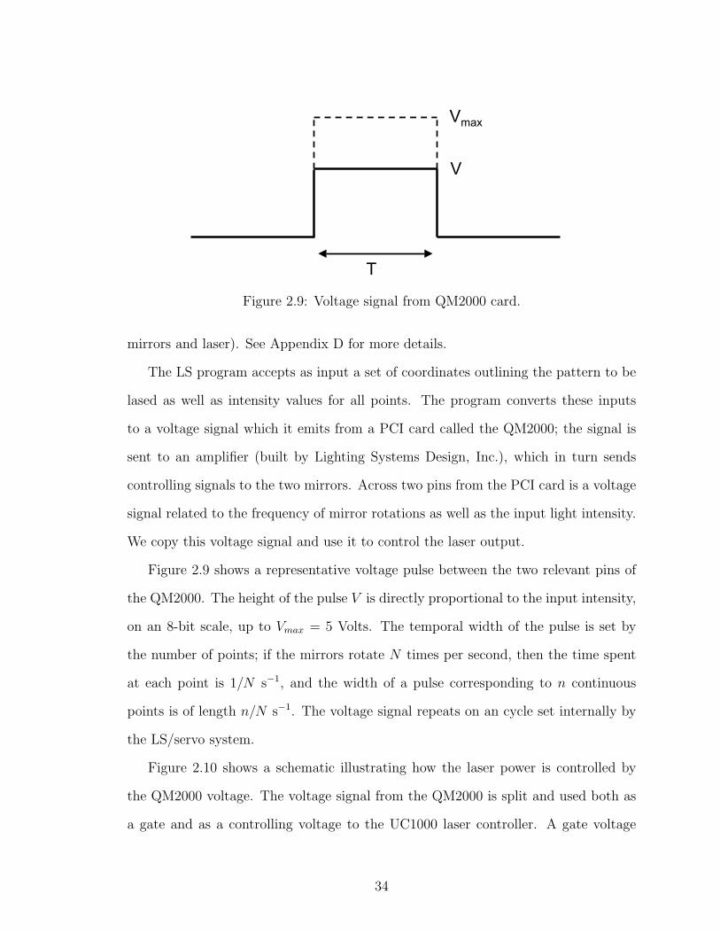
Vmax

V

T

Figure 2.9: Voltage signal from QM2000 card.

mirrors and laser). See Appendix D for more details.

The LS program accepts as input a set of coordinates outlining the pattern to be

lased as well as intensity values for all points. The program converts these inputs

to a voltage signal which it emits from a PCI card called the QM2000; the signal is

sent to an amplifier (built by Lighting Systems Design, Inc.), which in turn sends

controlling signals to the two mirrors. Across two pins from the PCI card is a voltage

signal related to the frequency of mirror rotations as well as the input light intensity.

We copy this voltage signal and use it to control the laser output.

Figure 2.9 shows a representative voltage pulse between the two relevant pins of

the QM2000. The height of the pulse V is directly proportional to the input intensity,

on an 8-bit scale, up to Vmax = 5 Volts. The temporal width of the pulse is set by

the number of points; if the mirrors rotate N times per second, then the time spent

at each point is 1/N s−1, and the width of a pulse corresponding to n continuous

points is of length n/N s−1. The voltage signal repeats on an cycle set internally by

the LS/servo system.

Figure 2.10 shows a schematic illustrating how the laser power is controlled by

the QM2000 voltage. The voltage signal from the QM2000 is split and used both as

a gate and as a controlling voltage to the UC1000 laser controller. A gate voltage

34

ControlVoltage

GateVoltage

QM2000 Board

UC1000Laser Controller

Laser

Figure 2.10: Schematic showing how the voltage from the QM2000 board is used, viathe UC1000 controller, to control the laser output.

above 3.5 V allows lasing, and the lasing power is proportional to the input control

voltage, on a 0-10 V scale.

Laser The CO2 laser is a model J48-1W from Synrad Corporation which has a

maximum power output of a few Watts. An interfacing control unit called a UC-1000

Laser Controller, made also by Synrad, was used to mediate the input voltage signal

(from the QM2000) and the outgoing signal to the laser. The UC-1000 sends a Pulse-

Width Modulated (PWM) voltage signal to the laser, based on a fixed 5-kHz cycle;

35

100% duty cycle is achieved by sending a constant logic-high signal, 0% duty cycle

by sending a constant logic-low signal, and a 50% duty cycle by sending a periodic 5

kHz high/low signal4. The duty-cycle set by the UC-1000 is controlled via the input

voltage signal from the QM2000 board, as shown in Fig. 2.10.

Servo Mirrors

In order to properly reflect infrared light, the original (silver-backed) mirrors attached

to the servo controllers were replaced. As part of the optical considerations, it was

best to find large mirrors to capture the full expanded laser beam, subject to the

constraint that the servo controllers have an expected inertial load; if the mirrors are

too heavy, the servo system will constantly overshoot the desired rotation. The best

solution is thin, gold-coated germanium wafer (any thin substrate would do). The

mirrors are squares approximately 1 cm × 1 cm, 250 µm thick.

4There is also a small tickle voltage the Controller maintains to keep the laser in a ready-to-lasestate.

36

CHAPTER III

PREPARING STRAIGHT ROLL PATTERNS

As a step toward understanding the mechanisms of instability in spatiotemporally

complex patterns, we first consider the instabilities of stationary straight roll patterns,

which can lead to a loss of time-independence and a possible transition to chaotic

behavior. For the range of control parameter ε used in this thesis work, natural

convection patterns are usually time-dependent and disordered. In order to study

the evolution of straight roll patterns near a secondary instability, an ordered pattern

must replace the initial pattern, and the state brought near a particular instability

in a controlled fashion. This chapter presents the methods by which straight roll

patterns are prepared for study. To facilitate this process, we prepare the straight

rolls in a rectangular convection cell. (Convection rolls have a natural tendency to

align at right angles to one of the sidewalls.) The experiments have been conducted

with a convection cell of lateral dimensions of 25 mm × 15 mm and a depth of 700

µm.

Pattern preparation consists of three parts. First is the mapping of the laser beam

to the convection cell; i.e., how rotations of the servo mirrors (see Chapter 2) “map”

laser light to a particular place in the convection cell. This mapping is crucial, as

the convective gas (SF6) absorbs the laser light locally; thus, the ability to exhibit

fine-tuned pattern manipulation is dependent on being able to direct the laser beam

to a particular location within the cell, with a high degree of accuracy. Given an

accurate mapping, an initial, idealized pattern is imposed over the existing, natural

convection pattern. This step is something of a brute-force method, in that the

actuation is nearly global over the convection cell and is implemented without regard

37

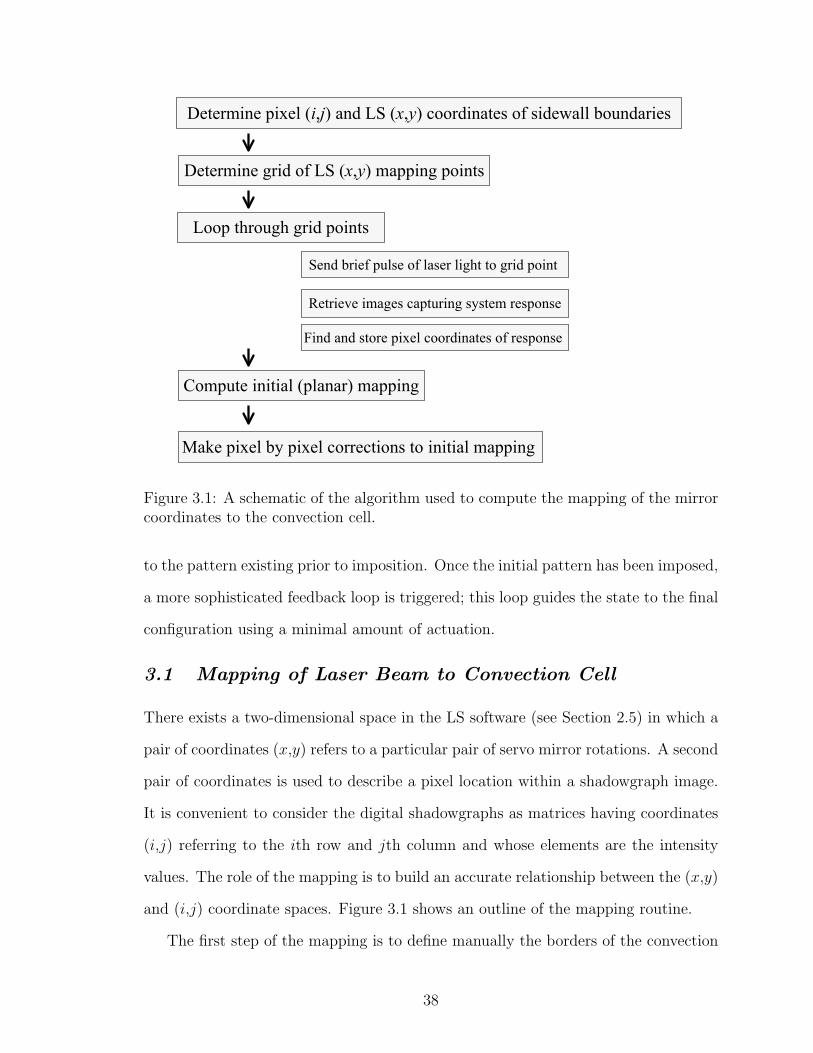
Determine pixel (i,j) and LS (x,y) coordinates of sidewall boundaries

Determine grid of LS (x,y) mapping points

Loop through grid points

Retrieve images capturing system response

Find and store pixel coordinates of response

Compute initial (planar) mapping

Make pixel by pixel corrections to initial mapping

Send brief pulse of laser light to grid point

Figure 3.1: A schematic of the algorithm used to compute the mapping of the mirrorcoordinates to the convection cell.

to the pattern existing prior to imposition. Once the initial pattern has been imposed,

a more sophisticated feedback loop is triggered; this loop guides the state to the final

configuration using a minimal amount of actuation.

3.1 Mapping of Laser Beam to Convection Cell

There exists a two-dimensional space in the LS software (see Section 2.5) in which a

pair of coordinates (x,y) refers to a particular pair of servo mirror rotations. A second

pair of coordinates is used to describe a pixel location within a shadowgraph image.

It is convenient to consider the digital shadowgraphs as matrices having coordinates

(i,j) referring to the ith row and jth column and whose elements are the intensity

values. The role of the mapping is to build an accurate relationship between the (x,y)

and (i,j) coordinate spaces. Figure 3.1 shows an outline of the mapping routine.

The first step of the mapping is to define manually the borders of the convection

38

cell. (This is simpler than trying to automate this step.) For rectangular sidewalls, it

simplifies things later to align the convection cell so that each sidewall segment lines

up with a either a constant row or constant column index of the shadowgraph images.

It is then convenient to define the cell boundaries by the four corners of the cell (for

circular cells, the alignment is not important, and the boundaries can be defined by

the row/column limits).

Four pairs of (x,y) coordinates are found that correspond roughly to the corners

of the convection cell. A brief laser pulse is directed into the convection cell and

absorbed by the SF6, causing a detectable localized response (see Fig. 3.2 and the

discussion immediately below). The coordinates are varied in a “guess and check”

manner until a response is observed near the cell boundary; these coordinates define

the boundaries of the cell in (x,y) space (only roughly, because there will ultimately

be a map over the entire convection cell).

Once the (x,y) borders have been defined, a grid of points over the domain of the

cell is compiled to which brief laser pulses are directed, serially. As each coordinate

pair is sent to LS to initiate the mirror rotation and lasing, the image-grabbing soft-

ware is given a signal to begin taking images, capturing the perturbation response.

The mapping algorithm then retrieves the small number of frames that hold the re-

sponse. It should be noted that the mapping is usually done slightly below the onset

of convection in order to isolate this response from any other convection pattern dy-

namics. Thus, the only frame to frame change should be due to the input disturbance.

Difference images are formed for all successive pairs of images; the one with the largest

rms intensity is assumed to contain the best signal of the perturbation response. An

example is shown in Fig. 3.2, where a bright spot in the middle of the image on the

left stands out above the raw shadowgraph image. The effect is much more visible

when a background image (no perturbation) is subtracted; this image is shown on

the right using a color map to further enhance the visibility of the structure. The

39

Figure 3.2: Shadowgraph snapshots during a mapping perturbation. The image onthe left shows the raw image containing the intensity change; the image on the rightshows the difference between the image on the left and a background image. Theimages show an area of ≈ 5d× 5d.

images have been cropped to show only a small portion of the convection cell, shortly

after the perturbation has been applied; we estimate the initial disturbance to be of

diameter ∼ d/2.

The pixel location with the largest peak intensity is found from the difference

images and the “center of mass” of the response is calculated, where the absolute

intensity (deviation of intensity from the mean) plays the role of the mass. These

“center of mass” pixel coordinates are stored, along with the original (x,y) coordi-

nates. This process is repeated over the (x,y) grid, thus producing a discrete map of

(x,y) coordinates to (i,j) shadowgraph locations over the convection cell.

A linear fit to the mapping data acts as a good first approximation of the relation-

ship between the pixel and LS coordinates; one can imagine this step as fitting the

data with (i,j,x) and (i,j,y) planes. The mapping thus takes the form of two matrices

of size equal to the shadowgraph dimensions: one contains the x coordinate for any

given (i,j) pair, the other contains the y coordinate for the same (i,j) pair. Now,

it is possible that the procedure that attempted to find the perturbation responses

40

resulted in some errors due to, for example, some small particle or air bubble in the

water flowing over the top boundary having passed in the view of the camera dur-

ing automated image capture. To eliminate those spurious data, the program cycles

through the data point by point, comparing the goodness of fit with and without the

point, and throws out those points that seem anomalous.

After this preliminary mapping, a finer mesh of (x,y) perturbation points over the

convection cell are used to make corrections to the linear approximation (the initial

set of points can be used if the initial grid resolution is high enough). The pixel

locations are found and stored in the same way as before for each point. Spurious

points are again excluded, but now by throwing away those that disagree strongly

with the initial mapping. For a given (i,j) pixel location, there is a corresponding

(x,y) pair of values from the initial fit. Nearby measurements from the finer mesh

may indicate that adjustments should be made to these values. Corrections are made

by summing over the adjustments indicated from each individual perturbation point,

with inverse distance weighting. All pixels are looped through and corrected, after

which the mapping is smoothed. This loop then repeats until both the x and the y

mappings converge.

Note that the final result is a mapping which allows the laser light to directed to

a location in the convection cell with sub-pixel resolution; in principle, the resolution

could be as high as desired, by increasing the number of mapping points. In practice,

it is suitable to use a few hundred points, which provides a resolution of ∼ 0.2 pixels

(about 1% of a pattern wavelength).

3.2 Straight Roll Imposition

After the mapping is complete, a straight roll pattern is imposed, the wavenumber of

which can then be controlled in order to guide the state to a given secondary insta-

bility; Fig. 3.3 shows a schematic summarizing the pattern imposition and control.

41

An idealized version of a straight roll convection pattern is first created digitally,

which amounts to specifying the pixel locations of the roll pairs by choosing some

pattern wavenumber and phase. This serves as the initial reference against which

captured shadowgraph images are compared. To impose this ideal pattern, the roll

positions are converted to output (x,y) coordinates via the mapping described above

and are drawn for a short time. Because the actuation is in the form of heating

from below, the pattern is drawn by sending a continuous line of laser light to each

desired location of hot upflowing fluid. The light is maintained at the upflow location

of each roll for about 1 s, after which the light is directed immediately to the next

upflow location in the desired pattern. After a full iteration through the rolls, the

lasing is turned off and a shadowgraph image is captured for comparison. If there

are discrepancies, the process is repeated, with the lasing time increasing progres-

sively after each iteration. If the process is successful, the algorithm calls for the next

step in the experiment, which is usually to maintain the imposed pattern and apply

perturbations, or to make adjustments, such as changing the pattern wavenumber.

Figure 3.4 shows shadowgraph snapshots during pattern imposition. The original,

natural pattern consists of evolving curved rolls and defects. Visible in the first few

frames is the increase in intensity where the laser light is being directed. Through

roll breakings and connections, the straight roll pattern emerges in about 30 - 60 s.

The physical walls can act as sources of defects and/or cause curving of nearby

rolls (due to the tendency of rolls to end at right angles to the walls). This is a

particular problem when controlling the pattern wavenumber because there is not

generally an integer number of rolls fitting neatly into the convection cell and therefore

it is difficult to enforce a constant wavenumber throughout the convection cell. To

minimize these sidewall effects, the pattern is established over the central region of

the cell, 2 wavelengths from either of the sidewalls in the wavevector region. The

direction of the wavevector along the longer side of the cell has been chosen to allow

42

(1) Create reference pattern

(2) Impose pattern

Iteratively lase upflow location for each roll

(3) Control boundary roll positions (feedback)

Grab shadowgraph image, compare against reference

If error is outside tolerance, change laser output

If error within tolerance, move boundary roll positions

Figure 3.3: The pattern control involves three main components, as indicated by thisschematic of the imposition/feedback algorithm.

43

Figure 3.4: Snapshots during straight roll imposition, at approximately 3 s intervals.The images show the full 25 mm × 15 mm convection cell.

more interior roll pairs to fit in the cell, typically 7-9.

3.3 Closed-loop Feedback Control

For the study of the straight roll pattern dynamics, it is desirable that the effect of the

optical actuation on the interior pattern dynamics is minimized. Thus, once the initial

pattern has been imposed successfully, actuation is restricted to the two outer-most

imposed convection rolls, which are thus deemed “boundary” rolls. Wavenumber

adjustments are made by moving the positions of these two rolls: bringing them

toward one another increases the wavenumber; moving them apart decreases the

wavenumber. The interior roll spacing adjusts to the boundary roll positions. A

feedback loop controls the relative positions of the boundary rolls and thus, in turn,

the interior roll spacing. This method of changing the interior wavenumber without

44

direct forcing of all the rolls is advantageous because it reduces the risk of causing an

instability in the bulk of the pattern.

In parallel with the feedback loop, the image-grabbing software takes shadowgraph

images and deposits them in a specificed directory shared by the feedback program

(running in Matlab). When a new image is detected, a subroutine is called that

performs an analysis to determine discrepancies between the reference and actual

convection pattern. A second subroutine uses these errors to determine the outputs

to be delivered to the laser controller and mirrors. The laser output affects the

convection pattern and this process repeats until the desired pattern is achieved.

One complete iteration of the feedback loop, including image analysis and calls to the

laser and mirrors, is achieved in a few tenths of a second, which is much faster than

the un-perturbed pattern evolution (as discussed below).

3.3.1 Shadowgraph Image Analysis

The information captured by the images is reduced to a set of pixel coordinates at the

center of each region of upflowing/downflowing fluid, and the image intensity along

each roll. These two signals are used for comparison to the ideal reference image.

As mentioned above, the rectangular sidewalls are positioned so that each of the

four sidewall segments aligns with a fixed row or column of the shadowgraph images.

The major benefit of this is that each of the ideal straight rolls can be referenced

with only one index (in most cases, a row index). Real rolls do not (generally) lie

exactly along a fixed row, possibly due to slight non-parallelism of the sidewalls, but

they do span the pixel columns of the convection cell. Figure 3.5 shows a straight

roll pattern and the (smoothed) intensity profile across the center pixel column. The

local maxima/minima of the intensity profile correspond to regions of hot and cold

flow, respectively. The row index of each roll, for this column, is determined by

finding locations of local maxima/minima of the intensity slices. The roll positions are

45

determined with sub-pixel resolution in one of two (similar) ways. When the intensity

profile is sufficiently smooth, a numerical derivative of intensity (with respect to pixel

position) can be computed and thus the maxima/minima found from places where

the derivative crosses zero. Or, motivated by the procedures in Ref. [47], quadratic

fits can be made locally to the intensity maxima/minima (once their positions have

been determined roughly). An example is shown in the zoomed-in intensity profile in

Fig. 3.6. The two methods give nearly identical results; we usually use the numerical

derivative, for computational ease. Thus, for a given column, the row positions of

all rolls can be calculated. Put together with intensity profiles over all columns, a

determination is made of each roll position across the domain of the cell.

This procedure of calculating roll positions is done in each pass of the feedback

loop and can be recorded for further use. When the program is set to change the

pattern wavenumber, the primary interest is the roll spacing of the boundary rolls, but

spacing of the interior rolls is also measured and will become important in Chapter 4.

3.3.2 Errors

The most significant source of error between the reference and observed convection

pattern is improper roll spacing, which is governed by the positions of the boundary

rolls. While there is a nominal desired pixel position for each boundary roll, it is more

appropriate to enforce not the absolute position but rather the pattern wavelength

(equivalently, the wavenumber). It must be noted that the sign of the error in roll

spacing is important physically. When the pattern is brought near an instability

boundary via a change in wavenumber, the natural tendency of the rolls is to relax

to a wavenumber closer to the center of the Busse balloon. When the wavenumber is

high, for example, and there is an error indicating the rolls are spaced closer together

than desired, it is usually appropriate to decrease, rather than increase, the laser

power. This holds for the converse situation at low wavenumbers. This allows the

46

50 100 150 200 250−1

−0.8

−0.6

−0.4

−0.2

0

0.2

0.4

0.6

0.8

1

Sca

led

inte

nsity

Pixel index

Figure 3.5: Shown above is the entire convection cell (and part of the cell boundaries,where the rolls terminate), showing the straight roll pattern under control (the curvedrolls at the top are outside the region of control). Underneath the roll pattern is aprofile of intensity values across the image, in the direction of the wavevector, asindicated by the line overlayed on the pattern.

47

125 130 135 140 145 150 155 160−0.8

−0.6

−0.4

−0.2

0

0.2

0.4

0.6

0.8

Pixel index

Sca

led

inte

nsity

Figure 3.6: Local quadratic fits to the intensity maxima/minima. The intensity valuesare given by the circles in blue; the fits are shown in red.

natural system dynamics to adjust the spacing when possible, which in turn minimizes

the amount of actuation required.

The shadowgraph intensity along boundary rolls is also monitored. At a high laser

power, such as when imposing an initial pattern, the effect of the optical actuation

is very apparent in the shadowgraph images through an increase in local intensity

(see the first few frames in Fig. 3.4). Near instability, or when probing system dy-

namics, this is undesirable because it indicates a possibly large disturbance to the

pattern. Therefore, an error is reported when the intensity of a boundary roll exceeds

a reference value (a good reference is the average intensity of a nearby, unperturbed

roll).

For each boundary roll, the position and intensity errors are normalized in order

to be combined into a single error; i.e., the error in roll position is normalized by the

pattern wavelength, and the intensity error is normalized by the intensity of a nearby,

un-perturbed roll. The two normalized errors are added with weighting coefficients

48

that reflect the relative error tolerances. Because the leading priority is to achieve the

desired roll positions, we set a lower tolerance for errors in roll positions. The actual

weighting values, found manually through trial and error, are those that consistently

give a positive error when the control begins to break down1.

The laser power is changed in response to the combined error; the power change

has the same sign as the error, but the magnitude depends on the current power

output: when the power is low (high), the control algorithm is most sensitive to large

positive (negative) errors. This design allows the algorithm to quickly adjust the laser

power to the appropriate level. The utility of this feature can’t be overstated, because

if the feedback program is delinquent in fixing an error in roll position, the roll may

begin to interact with grain boundaries emanating from the sidewalls (see the grain

boundaries in the images of Figs. 3.4 and 3.5); on the other hand, over-forcing due

to a large laser intensity can initiate instabilities. Either of these cases likely leads to

dynamics of the interior rolls and a loss of the straight roll pattern.

In addition to changes in the laser intensity, adjustments may be made to the lased

roll positions. Initially, laser light is directed to the nominal positions of the hot upflow

of the boundary rolls. When there is an error between the observed and reference

upflow position, the nominal position is moved slightly, opposite the direction of

error. These small changes are made in each iteration of the loop and have the effect

of moving the actual boundary roll position more quickly than an increase in power

alone. When the spacing between the boundary rolls and the adjacent interior rolls

assumes the desired value, the nominal boundary roll positions are updated with the

actual positions. This allows the overall straight roll pattern to drift by some small

amount, which is advantageous in that it may require less actuation to maintain the

1The approach here is that it is not necessarily the magnitude of the combined error that ismost important; rather, it is the sign of the error. With a very rapid feedback loop, many smalladjustments can have the same effect as a small number of larger adjustments. In this way, a highanalysis speed can, to a certain degree, make up for a lack of sophistication in the correction scheme.

49

boundary rolls at certain locations than others (due to interaction with the grain

boundaries, for example).

Error Tolerance The tolerance for errors in the roll spacing is set to a constant

0.2 pixels, as dictated partly by the resolution in the laser mapping and in part by

what has been shown to be achievable. This is only a small fraction of the pattern

wavelength, less than 2% even at the largest wavenumbers (smallest wavelengths).

When the spacing falls within this tolerance, the next step in the pattern control is

triggered: either a further change in the pattern wavenumber or the application of

selected perturbations, as discussed in Chapters 4 and 5.

3.3.3 Control near Boundaries

The physical sidewalls of the convection cell can be sources of forcing, due to the mis-

match in conductivity, and can therefore introduce defects at the boundary through

the joining of existing rolls or introduction of new rolls. Generally, these defects will

glide across the cell domain and be carried out by the opposite sidewall, with the fi-

nal result that the pattern wavenumber is changed. Therefore, when the wavenumber

set-point is sufficiently high or low (the state is very near instability), the positions

of the convection rolls near the sidewalls are monitored and controlled in a similar

fashion to the boundary roll positions.

3.3.4 Approaching Instability

The initial pattern wavenumber is chosen to be within the stable band (for a given

ε), and the state is brought near instability by either an increase or decrease in

wavenumber. Because the wavenumber is controlled via the positions of the two

boundary rolls, time must be allowed for the interior pattern to equilibrate after a

change in the boundary roll spacing. The vertical diffusion time tv = d2/ν is the

typical time scale over which local changes in the pattern occur, due to thermal or

50

viscous diffusion (for Pr ≈ 1, tv can be estimated using either ν or κ; we use the

smaller of the two). Changes to the global pattern can be expected to occur on

a timescale of th = Γ2tv, where Γ is the cell aspect ratio and th is defined as the

horizontal diffusion time. For a straight roll pattern of N rolls under control, the

distance from the center of the pattern to one of the boundary rolls isN

2λ, where

λ is the pattern wavelength. Typically, λ ∼ 2d, so we can define an aspect ratio of

the controlled pattern by Γ ∼ N

2(2d) = N . Thus, the timescale over which we can

expect the pattern to equilibrate is about N2tv. In our straight roll experiments, tv

is around 2.7 s, and we have 7-9 roll pairs, meaning the pattern equilibrates on the

order of a few minutes.

Changes in the wavelength are made in increments of the error tolerance (see

above), a very small percentage of the pattern spacing. Rather than wait 2-3 minutes

before every small change is made, however, the boundary roll positions are allowed

to be incremented as soon as their positions fall within the error tolerance, as long

as the pattern is far from instability. This procedure may cause transient uneven

spacing, but patterns ultimately are allowed to equilibrate over several minutes. As

the pattern nears instability, the time between spacing adjustments is progressively

lengthened.

51

CHAPTER IV

PERTURBATION LIFETIMES

The Busse balloon predicts an area of (q, ε) space in which ideal straight roll patterns

are predicted to be linearly stable; i.e., infinitesimal disturbances are expected to

decay. The secondary instability boundaries are defined by the (q, ε) values at which

patterns are predicted to be marginally stable. In between, we expect the time scale

over which disturbances decay to be related to the distance from instability. For a

small modulation about a stationary roll state in the vicinity of a secondary instability,

the rate at which the modulation decays is expected to be linear in the phase-space

distance from instability [48, 5]. (Basically, one can linearize the disturbance about

the bifurcation point.) In RBC, distance from bifurcation is usually considered in

terms of a temperature difference, just as ε = ∆T/∆Tc − 1 measures the distance

from onset of the primary instability. By using optical actuation, however, we have

both ε and the wavenumber q as control parameters that can be used to guide a stable

pattern toward a given instability boundary.

In this Chapter, we present the decay rates of disturbances to an ensemble of

prepared straight roll patterns at fixed ε, over a range of wavenumbers. This serves

both as an efficacy test of our experimental method of pattern manipulation near

instability as well as providing an experimental measurement of distance from one of

the more prevalent instabilities, the skew-varicose instability to roll regions of high

wavenumber. This measurement sets the stage for Chapter 5, wherein the modes

responsible for disturbance dynamics are determined experimentally.

52

4.1 Experimental Procedure

Using the feedback control algorithm described in Chapter 3, a straight roll pattern

is prepared with a given wavenumber. Once the pattern adopts the wavenumber

set-point, within some tolerance (see Chapter 3 for details), a subroutine is triggered

from within the feedback program to construct a detailed wavenumber field of the

pattern. This field is computed via the positions of all convection rolls in the pattern,

determined from continual shadowgraph image analysis. While the local wavenumber

is related to the local curvature, we find it more convenient, and equally informative

for our uses, to consider the local wavenumber defined by the spacing of adjacent con-

vection rolls. Distances between local intensity maxima/minima define wavelengths

(rather, half-wavlengths) at discrete positions, and interpolation builds a wavenum-

ber field over the full pattern domain. Figure 4.2 shows a straight roll pattern; shown

in Fig. 4.3 is the corresponding wavenumber field, where the approximate positions

of the hot upflow regions of the pattern have been marked by dashed lines. Note

that the wavenumber values given are non-dimensionalized in terms of the cell depth,

q = 2π/(λ/d).

Visible from the wavenumber field are small differences in the local roll spacing,

even over the length of two adjacent rolls. However, most of the variation is toward

the top and bottom of the image, where the boundary rolls are located; in the interior,

the spacing is relatively even. A probability distribution of all measured waveumber

values is shown in Fig. 4.4; the standard deviation is computed to be 0.10, only about

the 4% of the mean, q = 2.64.

The localized skew-varicose (SV) instability usually occurs in regions of large

local wavenumbers [49] (considering the bulk, that is, away from the boundaries). It

is thus reasonable to expect perturbations applied near maxima of the wavenumber

field will tend to excite the least-stable mode of the system corresponding to the

localized skew-varicose instability. We observe that perturbations directly between

53

1.5 2 2.5 3 3.5

0

1

2

3

SV

OSC

ECK

CR

q

ε

Lifetime Measurements

Figure 4.1: The Busse balloon showing various instabilities (CR, cross roll; ECK,Eckhaus; SV, skew-varicose; OSC, oscillatory) of the straight roll state, at a Prandtlnumber of 0.84, as in our experiments. The high-wavenumber region under study hasbeen highlighted.

54

Figure 4.2: An image showing the straight roll pattern under control.

55

Pixel index across cell

Nom

inal

rol

l loc

atio

ns

Local wavenumber of straight roll pattern

20 40 60 80 100 120 140

q

2.4

2.6

2.8

3

3.2

3.4

3.6

3.8

Figure 4.3: The local wavenumber field computed for the straight roll pattern inFig. 4.2. The dashed lines indicate the approximate locations of upflowing fluid. Thecolormap scale has been chosen to match that of Fig. 4.6.

56

2.4 2.5 2.6 2.7 2.8 2.9 30

0.2

0.4

0.6

0.8

1

Wavenumber PDF

Rel

ativ

e oc

curr

ence

Local wavenumber q

Figure 4.4: The probability distribution of local wavenumbers, as measured from thepattern in Fig. 4.2.

57

Figure 4.5: A pattern shortly after a point perturbation to the center cold roll (darkregions are cold down-flow; bright regions are warm up-flow).

adjacent regions of hot upflow are most likely to cause an instability; this makes

intuitive sense, as one can imagine that this type of perturbation acts to add another

region of upflow and thus increase the pattern wavenumber further. We therefore

find the location in the central portion of the pattern (away from the boundaries)

with the minimal separation between adjacent hot regions and apply a controlled

perturbation to the region of cold flow directly between. The perturbation is in the

form of heating of a single point in the pattern for about 100 ms, which results in

an initially axisymmetric disturbance of diameter ∼ d/2 = 350 µm. A stable pattern

exhibits a visible response to the perturbation but relaxes to the pre-perturbation

pattern after some period. The shadowgraph snapshot in Fig. 4.5 shows an example

of a pattern response shortly after a perturbation; note the center two rolls of the

pattern appear to bend toward one another, while the rest of the pattern deviates

much less from an ideal straight roll pattern.

4.1.1 Perturbation Strength

Necessarily, the applied perturbations are finite amplitude, as they need to be of

large enough amplitude to overcome the modal damping and cause a visible pattern

58

Pixel index across cell

Nom

inal

rol

l loc

atio

ns

Local wavenumber of straight roll pattern

20 40 60 80 100 120 140

q

2.4

2.6

2.8

3

3.2

3.4

3.6

3.8

Figure 4.6: A local wavenumber field immediately following a perturbation. As inFig. 4.3, dashed lines indicate the approximate locations of upflowing fluid in the basestate.

59

response. However, a sufficiently strong perturbation may cause the pattern to un-

dergo an instability; this is of particular concern when the pattern is already near

an instability boundary and the modes are weakly damped. The amplitude of com-

promise is one that results in a brief period of nonlinear evolution, followed by linear

decay. To account for any drift in laser intensity (from, say, a small change in the

length of the laser’s resonance cavity), we find it best to start with small perturba-

tions, lasting ∼ 100 ms, and then slowly increase the duration of the pulse if the

system response is weak.

4.2 Lifetime Measurements

Disturbance lifetimes are computed from snapshots of the pattern following a pertur-

bation (see Fig. 4.5), as the pattern displays some dynamical response before relaxing

back to the stationary state. Two related signals that can be used to define a life-

time are the rms intensity and the Fourier intensity, each of which can be computed

directly from the images. We have chosen to use a third method, however, due to

one significant drawback of either of these intensity measurements. Namely, there is

an arbitrary choice of area from which either intensity signal is computed. A cleaner

signal is obtained from considering a larger area, but because of the localized nature

of the excited structures, pixels far from the central point of the perturbation are un-

likely to contain much relevant information; conversely, an intensity signal computed

from very few pixels is subject to a larger degree of fluctuation. (This is another way

of saying that, a priori, the spatial extent of the excited structure is unknown.)

A different measure gives a clean and more reproducible signal. When the cold

fluid between two adjacent hot upflow regions is perturbed, the upflow regions appear

to bend toward one another and then relax back to their original positions at some

rate that is dependent on distance from instability. Recall from Chapter 3 that the

roll positions are computed as a step in the pattern control loop; the system response

60

is visible from this measurement in the form of a large dip in the local spacing. This

response is most noticeable from the computed wavenumber field; Fig. 4.6 shows a

wavenumber field following a point perturbation between regions of hot up-flowing

fluid. Notice the spatial-localization of the disturbance.

A one-dimensional signal is formed by the separation of the upflow regions at

their nearest point. This local spacing is converted to a wavenumber, which displays

a large peak when or shortly after the perturbation is applied, followed by smooth

decay to the equilibrium value over time. Note that because only the relative positions

of the rolls is important in this measurement, any small amount of overall pattern

translation (say, from a vibration of the apparatus) is ignored. The latter portion is

well fit by one exponential term: q(t) = q0 +Q exp(−t/τ), where q0 is the relaxation

value, Q is a perturbation amplitude, and we define τ as the disturbance lifetime

(equivalently, τ−1 is the disturbance decay rate). An example is shown in Fig. 4.7.

Deviation from the fit at the beginning of the decay, which becomes more noticeable

near instability, is attributed to nonlinear evolution. The linear decay is typically on

the order of a few to many seconds. In this example, the relaxation value is q0 = 2.76,

and the decay rate is τ−1 = 0.31 s−1. In any cases where the applied perturbation

causes the local wavenumber to shift (the pattern relaxes to a spacing much different

than the initial one), those measurements are not used.

4.3 Results

The measured decay rates are shown in Fig. 4.8, as a function of the local wavenumber,

with a linear fit. The scatter between individual points indicates well the uncertainty

in any one lifetime value, which is estimated from multiple fits of any given response

signal (using various segments of the full signal) to be ' 10%. This repeatability

of the measurements and the linear profile of the decay rates over the wavenumber

range are good indicators that the straight roll patterns have been prepared without

61

0 5 10 152.5

3

3.5

4

4.5

5

Time (s)

Loca

l Wav

enum

ber

MeasurementExponential Fit

Figure 4.7: The local separation of adjacent upflow regions over time, after a pertur-bation to the cold downflow region in between. The red line shows an exponentialfit.

62

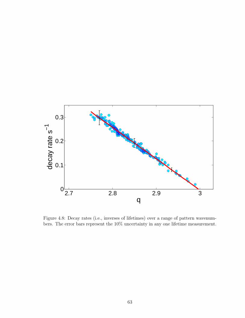
2.7 2.8 2.9 30

0.1

0.2

0.3

q

deca

y ra

te s

−1

Figure 4.8: Decay rates (i.e., inverses of lifetimes) over a range of pattern wavenum-bers. The error bars represent the 10% uncertainty in any one lifetime measurement.

63

introducing unwanted disturbances, such as thermal inertia effects from perturbative

boundary heating.

The perturbation decay rate decreases by an order of magnitude over the range

of wavenumbers studied here. This continuous slowing down of the dynamics near

the expected instability implies that we are indeed capturing a signature of the least-

stable mode, which is confirmed by the fact that localized skew-variocse instabilities

occur when attempting to increase the wavenumber beyond this range. Perturbations

to patterns with q slightly below the smallest values given here decayed too rapidly to

retrieve a reproducible lifetime measurement; this is consistent with the phase space

location being in the center of the Busse balloon, where patterns are far from any

secondary instability, but it leaves open the possibility of a dominant mode in this

lower range of q distinct from the one captured by these lifetime measurements.

The point at which the linear fit to the decay rates crosses zero indicates the

critical value1 of the local wavenumber, where perturbations are not expected to

decay, qc = 3.00; this marks the boundary of the localized skew-varicose instability

at ε = 0.60. We can see from the Busse balloon (Fig. 4.1) that this value is slightly

smaller than that prediced from global instability of an ideal, infinite pattern at this

ε (qc = 3.15). This discrepancy is unsurprising, insofar as the spatial-localization of

the pattern response to perturbation indicates that the critical mode is not globally

extended, as suggested by the Busse balloon analysis, and therefore one might expect

the critical roll spacing to differ somewhat from that of the idealized pattern.

The exponential decay suggests that there is a single long-lived mode being excited

from perturbations to downflow regions of these high-q patterns, but it is unclear from

these results if perturbations of this type will generally excite the dominant spatially

localized modes. Moreover, it is desirable to characterize the spatial structures and

1This critical wavenumber for the onset of the secondary skew-varicose instability should not beconfused with the value of the critical wavenumber for the onset of convection.

64

time scales for not only the dominant modes but other important, sub-dominant

modes. That is the subject of the next Chapter.

65

CHAPTER V

MODAL EXTRACTION

5.1 Introduction

In many systems, analysis of infinite, ideal patterns can provide a description of dy-

namics and pattern selection (e.g., the Busse balloon), but this approach can fail for

systems with boundary forcing or in states far from the initial pattern onset. As dis-

cussed in the Introduction, and as illustrated in the previous chapter, one consequence

of imperfect patterns is the spatial localization of the dominant system modes and

thus spatially localized instabilities. In convection states exhibiting persistent chaos,

such as the spiral defect chaos state (see the Introduction), we indeed do observe

continual defect growth/annihilation on a local scale. The introduction of defects to

an ordered state (straight rolls) can result in a cascade of instabilities that lead to

global chaotic behavior, as in the case of a transition from a straight roll to the SDC

state. It is therefore worthwhile to understand the mechanisms of spatially localized

instabilities quantitatively.

In this chapter, we present the experimental and analysis procedures that we

have developed for extracting the dynamical modes governing secondary instability

of the straight roll state. Our approach uses the common idea of using an ensemble of

states with nearby initial conditions to understand the important dynamical degrees of

freedom, but is novel in that our ensemble is prepared experimentally. We repeatedly

prepare a base straight roll pattern, to which selected perturbations are applied, giving

an ensemble of patterns evolving from a set of nearby initial conditions. From the

ensemble of different pattern evolutions, we compute a small set of basis patterns that,

together, are sufficient to describe the observed pattern dynamics. By representing the

66

evolutions of all ensemble members in this low-dimensional basis computed directly

from the different pattern evolutions, (rather than, say, a Fourier basis), we are able

to construct a matrix representation of the operator that governs the evolution of

disturbances to the base state. This eigenmodes and eigenvalues of this evolution

operator, which is constructed from the experimental measurements, give us directly

the dynamical modes of the base state as well as the growth rates of those modes.

We present the spatial modes and growth rates extracted from experiments at

three different locations in (ε, q) parameter space; these locations are shown in the

context of the Busse balloon for our experimental conditions (Pr = 0.84) in Fig. 5.1.

Note that the measurements of perturbation lifetimes in Chapter 4 were taken at the

same ε and at wavenumbers surrounding DI . To illustrate the analysis procedure, we

show how the intermediate steps apply to the ensemble at DI ; many of the conclusions

will hold for all three ensembles, but any significant differences in the results of a given

analysis step from one ensemble to another will be noted. Many images showing

portions of the straight roll patterns have been cropped to show a square region of

the pattern under control, usually 7-9 wavelengths; recall that all wavenumbers are

given in non-dimensional units: q = 2π/(λ/d).

5.2 Creation of Perturbation Ensemble

A given perturbation (as described in Section 4.1) excites one or more system modes.

How many are excited, and which ones, may depend on the size, strength, and lo-

cation of the perturbation. In order to excite all the dominant modes governing

disturbances to a pattern, perturbations of differing strength are applied to evenly

spaced points across a pattern half-wavelength (see Fig. 5.2). Note that all spatially

localized modes are related to those excited from this ensemble through symmetries

(see below) of the ideal straight roll pattern; an ensemble across a half-wavelength

therefore comprises a “minimal” ensemble (however, as it turns out, it is useful to

67

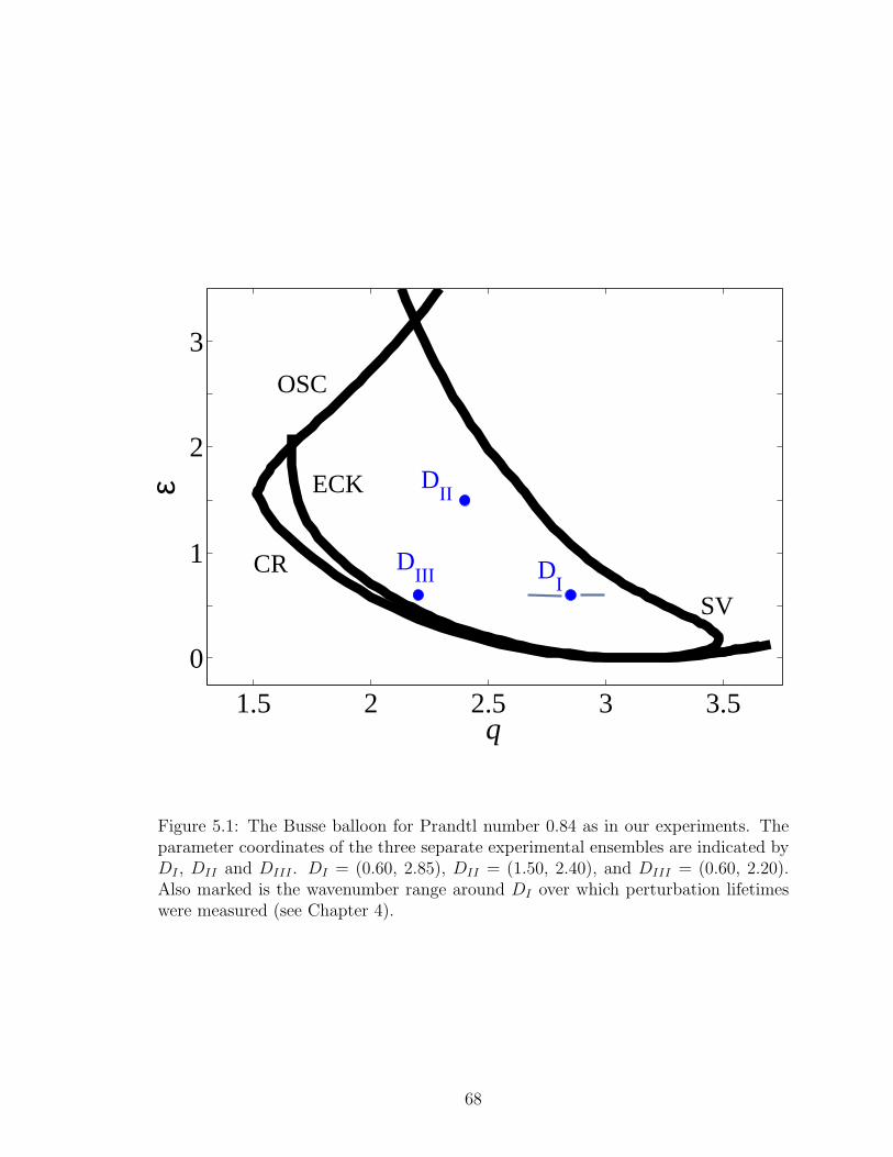
1.5 2 2.5 3 3.5

0

1

2

3

DI

DII

DIII

SV

OSC

ECK

CR

q

ε

Figure 5.1: The Busse balloon for Prandtl number 0.84 as in our experiments. Theparameter coordinates of the three separate experimental ensembles are indicated byDI , DII and DIII . DI = (0.60, 2.85), DII = (1.50, 2.40), and DIII = (0.60, 2.20).Also marked is the wavenumber range around DI over which perturbation lifetimeswere measured (see Chapter 4).

68

Figure 5.2: Perturbations are applied at different points along the direction of thepattern wavenumber (indicated by the arrow); perturbations across a half-wavelengthconstitute a minimal set.

consider a more extended ensemble). We define a grid of six perturbation locations

over a pattern half-wavelength; because the spatial extent of the laser is 10% or more

of the pattern wavelength (or 20% of the half-wavelength) in all cases reported here,

there is no benefit from a finer partition. The perturbation locations are determined

relative to the measured position of a central roll pair of the pattern, accounting for

any slow drift of the pattern. While it is not known a priori how many distinct modes

we may be able to extract, it is reasonable to expect the number to increase with the

ensemble size. We therefore impose a large number (∼20) of perturbations at each of

the pre-determined locations.

5.3 Shadowgraph Image Processing

When a perturbation is applied, it excites modes of the system which modulate

the base straight roll pattern. Shadowgraphs capture the pattern evolution after

an imposed disturbance and thus contain snapshots of the composite structure of the

excited modes over time. The following steps are taken to prepare the shadowgraphs

for analysis.

69

5.3.1 Spatial Filtering

While the effect of the perturbations is visible on the raw shadowgraph images, the

structures of the excited modes can be seen more clearly by subtracting the station-

ary straight roll pattern from all images following the perturbation. In Fig. 5.3 we

show a pattern immediately following a perturbation and then a short time later.

For comparison, the images are also shown after the straight roll pattern has been

subtracted. A spatial window centered around the perturbation point is applied to

all images to filter out intensity fluctuations far from the response. The images are

then Fourier filtered. Rather than apply a wavenumber filter of the Fourier spec-

trum (which would eliminate structures at some length scales), we elect to keep the

most dominant Fourier modes over the entire spectrum. An FFT is applied to each

shadowgraph image capturing a given perturbation decay. The sum of Fourier am-

plitudes over the time series provides a Fourier spectrum representative of the most

important modes present in the perturbation trajectory. Only those Fourier modes

with amplitudes greater than 10% of the maximum are retained; thus, the number of

Fourier modes is reduced from order 104 (the number of pixels in the original images)

to the same few hundred over all snapshots of the perturbation trajectory (we have

confirmed that including slightly more or fewer Fourier modes does not change the

results). Figure 5.4 shows the decay of excited structures after perturbation to a

pattern at DI after the images have been spatially filtered.

5.3.2 Temporal Filtering

Due to memory limitations of our computer, the frame rate of the image-capturing

software can fluctuate, at times, up to 30% of the nominal frame rate of about 10

frames per second. Although this amounts to a variation of less than 1/10 of a second

between subsequent frames, small temporal errors will cause identical perturbations

70

Figure 5.3: Images showing how the structures excited by perturbations can be vi-sualized by subtracting off the stationary straight roll pattern. On the top are theraw images immediately following a perturbation and then at a short time (about1 s) later. On the bottom are the same images after the straight rolls (with noperturbation) have been subtracted.

71

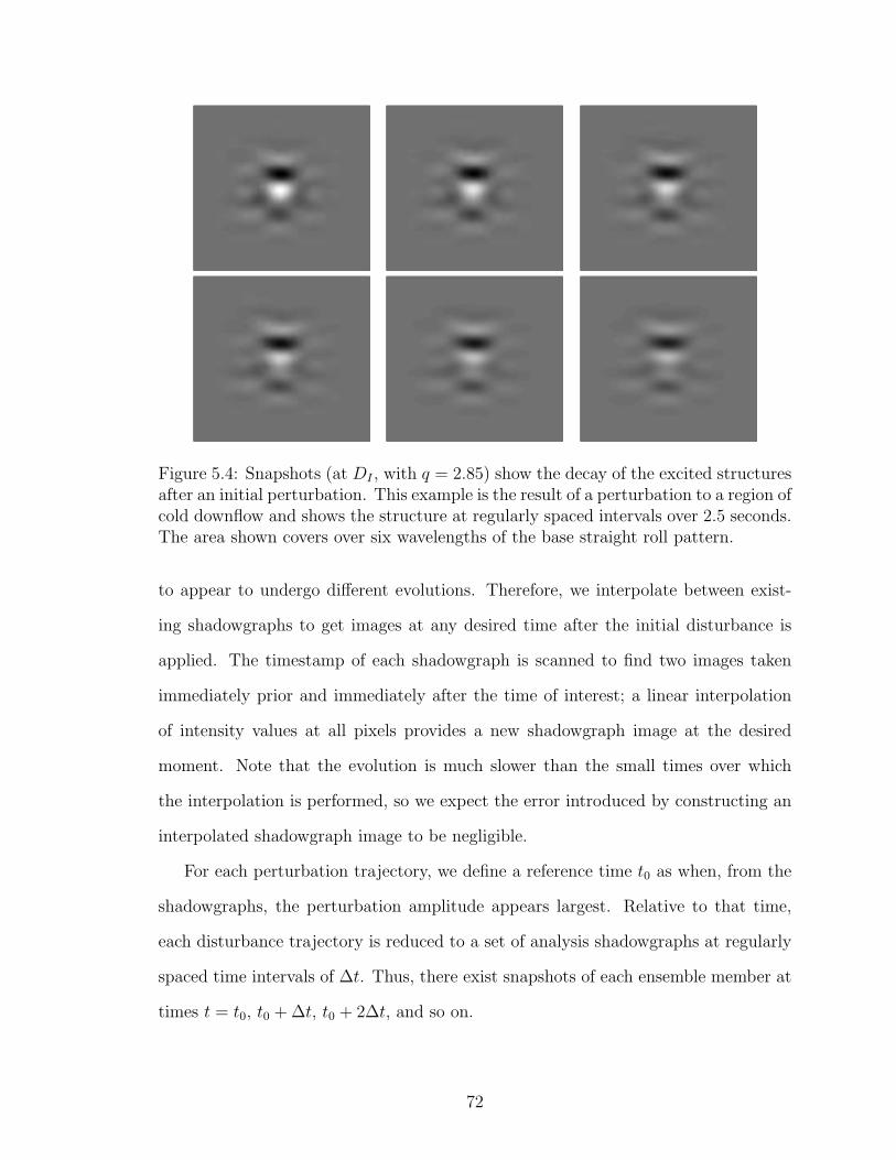
Figure 5.4: Snapshots (at DI , with q = 2.85) show the decay of the excited structuresafter an initial perturbation. This example is the result of a perturbation to a region ofcold downflow and shows the structure at regularly spaced intervals over 2.5 seconds.The area shown covers over six wavelengths of the base straight roll pattern.

to appear to undergo different evolutions. Therefore, we interpolate between exist-

ing shadowgraphs to get images at any desired time after the initial disturbance is

applied. The timestamp of each shadowgraph is scanned to find two images taken

immediately prior and immediately after the time of interest; a linear interpolation

of intensity values at all pixels provides a new shadowgraph image at the desired

moment. Note that the evolution is much slower than the small times over which

the interpolation is performed, so we expect the error introduced by constructing an

interpolated shadowgraph image to be negligible.

For each perturbation trajectory, we define a reference time t0 as when, from the

shadowgraphs, the perturbation amplitude appears largest. Relative to that time,

each disturbance trajectory is reduced to a set of analysis shadowgraphs at regularly

spaced time intervals of ∆t. Thus, there exist snapshots of each ensemble member at

times t = t0, t0 + ∆t, t0 + 2∆t, and so on.

72

5.4 Construction of Karhunen-Loeve Basis

A Karhunen-Loeve (KL) decomposition of the perturbation ensemble creates a set of

basis modes in which to embed all perturbation trajectories. Note that the KL basis

modes should not be confused with system eigenmodes; the KL modes are simply a

choice of basis in which to represent all the perturbation evolutions. The essence of a

KL decomposition is to build from a measurement a set of basis modes that capture

the correlations present in the data. In our case, the measurement is a set of images

showing the evolution of an ensemble of structures excited by perturbations. In this

measurement set, there will be some pixel-to-pixel correlations across different images

(for example, a particular group of pixels may all take on large intensity values in

select images). A matrix of these pixel-to-pixel correlations is formed: this is the

covariance matrix. An eigenvalue decomposition of this covariance matrix provides a

set of KL modes, with each mode formed by a combination of pixels that are together

correlated. The KL modes are ordered by the respective fraction accounted for of

the total amount of measurement correlation; the modes themselves are minimally

correlated.

We wish to reduce the correlations across excited structures present in the pertur-

bation ensemble; the KL modes that capture the bulk of the correlation will then form

the embedding basis. Note that, in contrast to the typical implementation of the KL

decomposition [50, 51], this reduces covariance over different initial conditions rather

than over time. This is an important difference, because time-averaged correlations

(over a single trajectory) sample different states and can neglect structures that, al-

though appearing infrequently (in time), have an important dynamical role [52]. Our

KL basis captures the different structures about a single state (i.e., the different ways

in which a pattern can change relative to a base pattern). Thus, our KL basis can be

considered to be more representative of the dynamical, rather than statistical, modes.

Let xi denote the intensity vector formed from a shadowgraph image capturing

73

the structures excited from the i-th perturbation. We then construct the N × M

matrix X,

X =

[x1 x2 · · · xM

]where M is the number of different initial conditions, and N , the number of rows,

is equal to the original dimension of the data, i.e., the number of image pixels. The

covariance matrix is then XXT, where XT refers to the transpose of X. The covari-

ance matrix has dimensions N ×N . Finding the eigenvectors and eigenvalues of this

large matrix (N ∼ 104, the number of pixels) is a daunting task; instead, we perform

an eigenvalue decomposition of the matrix XTX, which has dimensions M ×M , with

M � N . If Λ is the diagonal eigenvalue matrix of XTX and V is a matrix with

columns filled by the eigenvectors, we can write XTXV = ΛV. Multiplying by X

on the left gives XXTXV = XΛV = ΛXV, from which we conclude that XV are

the eigenvectors of the original covariance matrix, sharing the same eigenvalue matrix

Λ. We therefore perform the computationally feasible calculation: we compute the

eigenvectors V of XTX and transform those vectors by multiplying on the left by X;

XV are the eigenvectors (KL modes) of the original covariance matrix XXT.

Together with the KL eigenvectors are the corresponding eigenvalues; the eigen-

value of a given KL mode indicates the fraction of the total variance accounted for

by that mode (more precisely, the eigenvalue should be normalized by the sum of all

eigenvalues). There exist as many basis modes as there are original measurements

(images). Modes with small eigenvalues are those that appear in few of the images,

and therefore add little to the description of the modal trajectories. Moreover, in-

cluding modes with very small contributions can contribute to spurious results, as it

effectively introduces a dimension into the analysis that likely has little dynamical

relevance. Again, it should be noted that although small-eigenvalue KL modes can

carry significant dynamical information in a time-averaged decomposition, we do not

expect this to be the case for our ensemble-average over nearby initial conditions,

74

where the slowest structural decay is likely due to the dominant modes of interest.

Accordingly, we limit our embedding dimension to the smallest number of modes that

capture 90% of the power of the KL eigenvalue spectrum.

While we are free to choose which of the ensemble images are used to construct

the KL basis, it is appropriate to use the images near the end of the perturbation

evolution, as this favors the longest-lived modal structures; other modes may be

present in the early snapshots but are of less interest because they decay rapidly.

5.4.1 Perturbation Averaging

At DI , 23 individual perturbations (varying only in amplitude) were applied at each of

the six perturbation locations of a pattern half-wavelength. As mentioned above, the

choice of the number of different perturbations locations is guided by the spatial extent

of the laser beam. A KL decomposition of the DI ensemble therefore provides up to

138 basis modes. However, as Fig. 5.5 shows, the variance is unevenly distributed; the

fraction of the total variance accounted for is plotted against the number of KL basis

modes. Recall that, in our formulation, the variance is across the spatial structures

present in the ensemble images. The first several modes account for over 50% of

the variance; this suggests that the perturbation structures can be described by a

lower-dimensional basis.

To isolate the possible dependence of the extracted modes and growth rates on

the perturbation amplitudes, we decomposed the full ensemble of initial conditions

into four sub-ensembles based on the maximum rms shadowgraph intensities. The

KL modes across sub-ensembles were consistent, indicating that, at least over the

perturbations considered here, there is no discernible dependence of the excited modal

structures on the perturbation strength. Therefore, in the interest of minimizing any

residual noise, all the perturbation trajectories at a given location are averaged; the

largest number of KL modes is then equal to the number of perturbation locations.

75

1 20 40 60 80 100 120 140

0.4

0.5

0.6

0.7

0.8

0.9

1

Number of KL basis vectors

Fra

ctio

n of

tota

l cov

aria

nce

Figure 5.5: The fraction of the total variance accounted for by the KL basis modesat DI as a function of the basis size.

76

1 2 3 4 5 60.7

0.75

0.8

0.85

0.9

0.95

1

Number of KL basis vectors

Fra

ctio

n of

tota

l cov

aria

nce

Figure 5.6: The fraction of the total variance accounted for by the KL basis modesat DI as a function of the basis size, after averaging perturbations at each respectivelocation.

The variance distribution for the resulting six KL basis modes at DI is shown in

Fig. 5.6. The corresponding basis images are shown in Fig. 5.7. The first few modes

account for over 90% of the variance; this result holds for all three data sets.

5.5 Determination of Modal Structures and Growth Rates

To avoid confusion, we change notation slightly to distinguish between vectors in

shadowgraph pixel space and those in the space spanned by the KL basis. Let b0 de-

note the disturbance following an initial perturbation, expressed in a low-dimensional

(KL) basis. After some time T , this state has evolved to bT . Then Ub0 = bT , where

U is the evolution operator. Using an ensemble of initial conditions we define

B0 =

[b0

1 b02 · · · b0

M

]

77

Figure 5.7: The KL basis images at DI . As in Fig. 5.4, the area shown covers oversix wavelengths of the base straight roll pattern.

and similarly,

BT =

[bT1 bT2 · · · bTM

]This gives the over-determined (least-squares) problem for the evolution operator

UB0 = BT , which is solved by U = BT (B0)−1

, where the reciprocal of B0 is taken

to refer to the generalized inverse of the non-square matrix.

During linear decay, each system eigenmode decays at a characteristic rate, so we

can also write Uei = exp(σT )ei, where ei are the eigenvectors and the eigenvalues λi

are related to the growth rates by λi = exp(σiT ).

Recall that we have, for each disturbance, snapshots at evenly spaced times over

the disturbance decay; we select from the series of snapshots of each perturbation evo-

lution an image representing the “initial” disturbance and, for convenience, re-label

the time of that image as t = 0. The snapshot representing the “final” disturbance is

then selected a time T later.

78

While these choices of “initial” and “final” times may appear arbitrary, they can

have measurable effects on the convergence onto system eigenmodes. Using snapshots

from the earliest stages of disturbance evolution may, for example, include nonlinear

evolution, which will affect the extracted modal structures and/or growth rates. On

the other hand, using snapshots long after the initial disturbance may result in the

strength of the captured signal to appear too weak to stand out from the background

noise.

With these possible effects in mind, the initial and final times are varied as a

measure of the robustness of the extracted modes. We find that there is a clear range

of 2-5 s over which the modal structures and the growth rates change little with

respect to changes in the initial or final image times. This yields an estimate of the

uncertainty of any one growth rate to be ∼ 10%.

5.5.1 Use of Pattern Symmetries

While the preliminary results suggest that the algorithm does indeed converge on

system eigenmodes, we observe that the dominant mode is extracted as part of a

complex conjugate pair. At DI , for example, the growth rate with largest real com-

ponent is σ = −0.13 ± 0.03ı s−1. While the proper interpretation of the imaginary

part of σ is as a temporal frequency, this would imply a period of multiple minutes;

the analysis takes place on the order of seconds, suggesting that we do not have the

resolution to detect temporal oscillation on that time scale, and that this imaginary

component may be spurious. To break the degeneracy of the real part of the leading

growth rate, we consider the system symmetries.

Considerations of symmetry are useful for determining allowed patterns and in

building a minimal description of the dynamics in both unbounded and bounded

79

“cold” symmetry plane

“hot” symmetry plane

Figure 5.8: Two symmetry planes are defined over a half-wavelength of the pattern,one at the center of (hot) upflowing fluid, the other at the center of adjacent (cold)downflowing fluid. Four symmetric versions of each disturbance are formed by de-composing the disturbance into even/odd structures about either symmetry plane.

systems. The straight roll pattern contains the following symmetries: discrete trans-

lational symmetry (periodicity) in the direction of the wavevector, translational in-

variance in the direction perpendicular to the wavevector, and reflection symmetries

across planes defined at the centers of hot/cold fluid. These symmetries are met ap-

proximately as long as the localized disturbances are far from the physical boundaries

and far from locations where actuation is applied to rolls under control. Specifically,

we examine the disturbance evolutions through the reflection symmetries by analyzing

disturbances applied across a full pattern wavelength.

All disturbances can be decomposed in terms of symmetries related to a roll pair.

We define two symmetry planes, one at the center of upflowing fluid, the other at

the center of adjacent downflowing fluid (see Fig. 5.8). We can therefore define four

symmetric versions of every initial disturbance, each even/odd about the hot/cold

symmetry planes. Each of the corresponding four subspaces is invariant: disturbances

retain their symmetry as they evolve.

The entire collection of initial and final conditions was decomposed using these

symmetries, producing four independent ensembles. All eigenmodes extracted from

the four ensembles are eigenmodes of the system, but in the cases when multiple

eigenmodes share an eigenvalue (growth rate), we eliminate redundant representations

80

by computing the most spatially localized eigenmode structure.

Fundamental Modal Structure We wish to group all extracted modes by

growth rates and define the fundamental mode as the most localized structure with

a particular growth rate. For a given growth rate, there may exist up to four dif-

ferent extracted modal structures, one from each of the four symmetrized ensembles

(although some symmetrized ensembles may not produce a mode with that growth

rate). We group all of these modal structures together with copies of the same struc-

tures translated by an integer number of pattern wavelengths. The fundamental

mode of a given group of modal structures is the linear combination of those struc-

tures which minimizes the p-norm, with 0 < p < 2. The p-norm of vector v, with i-th

component vi, is defined as (∑i

vpi )1/p. Recall that eigenmode structures are defined

up to an overall multiplicative constant: subject to an enforced normalization of the

2-norm (what would generally just be called the magnitude), minimizing the p-norm

(p < 2) produces a structure with the fewest number of non-zero components1. In our

case, each component is a pixel element, so we are essentially minimizing the number

of pixels that contribute to the fundamental modal structure. The linear combina-

tion of input modes is defined by a set of coefficients {ck} describing the weight of

each of the respective modal structures on the composite structure: x =K∑k

ckek. A

minimization routine was used to converge on the ck.

5.5.2 Results

In all cases, one mode was extracted from each of the symmetrized ensembles; a mode

even/odd about the hot/cold symmetry plane. There were two distinct growth rates

extracted, each shared by a pair of the structures.

1Consider a simple example in two dimensions to illustrate this point: a vector with one non-zero

component, x = (1, 0), and another vector with two non-zero components, y = (1√2,

1√2

). Both

have 2-norms (magnitudes) equal to 1, but x has a smaller p-norm for any p < 2.

81

High Wavenumber The four symmetrized modes at DI are shown in Fig. 5.9,

with growth rates σ1 = -0.13 s−1 and σ2 = -0.70 s−1. A second set of perturbations

at high q was performed at DII , with ε increased relative to DI . Again, two distinct

growth rates are extracted; σ1 = -0.15 s−1 and σ2 = -0.55 s−1. Mutual projections

of the modes extracted at DI and DII indicate that the spatial structure of the

two dominant modes changes little (after scaling by the wavelength) between these

two locations. In Fig. 5.10, we compare a pair of symmetrized modes from the two

ensembles, after the images have been scaled by the respective pattern wavelengths.

There is also, in both cases, a large separation between the two growth rates. This

suggests we can identify the dominant mode as the one representing the secondary

instability at the high wavenumber boundary. The fundamental dominant and sub-

dominant modes are given in Fig. 5.13. As the lifetime measurements suggested, the

least-stable mode tended to be excited from perturbations to cold downflowing fluid.

Note, however, that while the structures excited from these disturbances are even

about the downflow symmetry plane, the most-localized representation of this mode

does not obey that symmetry. The sub-dominant mode tended to be excited from

perturbations to hot fluid. The structure of the dominant mode is consistent with

a skew-varicose type instability. Figure 5.12 shows as an example the input modal

structures for determining the fundamental representation of the dominant mode.

Low Wavenumber We also created an ensemble of perturbations to a low-

wavenumber pattern, at DIII . As in the other cases, four symmetric modes were

extracted; two dominant modes share a growth rates σ1 = -0.20 s−1 and the sub-

dominant modes have σ2 = -0.27 s−1. Shown in Fig. 5.11, the spatial structure of

the dominant mode does not resemble any of the previously extracted modes, while

the sub-dominant mode resembles the sub-dominant mode extracted at both DI and

DII . The two fundamental modes are shown in Fig. 5.14. The closeness of the growth

82

Figure 5.9: The four symmetric modes extracted at DI . The top two images showthe pair of structures sharing the largest growth rate; the two sub-dominant modesare shown below. Dashed lines mark the approximate locations of the hot upflowof the underlying base state; cold fluid lies between the dashed lines. (The distancebetween adjacent dashed lines is one pattern wavelength.)

83

Figure 5.10: On the left, versions of the dominant (top) and sub-dominant (bottom)modes extracted at DI . Next to these for comparison are modes extracted from thesecond high-wavenumber ensemble at DII . The images have been scaled to show thepatterns, over six wavelengths, using the same image size.

84

rates is consistent with the existence of two low-wavenumber instability types of the

unbounded system that occur at very nearly the same parameter values, namely, the

Eckhaus and cross-roll instabilities (see the Busse balloon in Fig. 5.1). The dominant

mode is again excited from perturbations to a downflow; we find experimentally that

sufficiently strong perturbations of this kind result in the growth of rolls perpendic-

ular to the base pattern. We therefore identify the dominant low-wavenumber mode

with the localized cross-roll instability and the sub-dominant mode with the localized

Eckhaus instability.

It is worthwhile to note that the leading modes at DI , DII , and DIII tended to be

excited from perturbations applied to cold fluid while the sub-dominant mode tended

to be excited via perturbations to hot fluid. As mentioned in the previous chapter,

this is unsurprising, as heating of cold fluid tends to reduce the amplitude of the

saturated roll state and can thus be seen as a destabilizing force.

Note that the symmetries imply that all extracted modes in each group can be

represented as linear superpositions of the fundamental mode along with its translated

and/or reflected copies. We verified that this is indeed the case as such representation

was accurate, with mutual projection > 0.94. Three examples of the least-squares

fits of more spatially extended modes are shown in Figs. 5.15.

5.6 Conclusions

The results presented indicate that two system eigenmodes describe the observed dy-

namics of any one location of phase space that was investigated. It is possible that

closer to instability, more strongly damped modes may begin to play a dynamical

role in the evolution of disturbances, but it is logical to expect modes to deform in a

continuous way and thus for the dominant modes to change little in the neighborhood

of any one (q, ε) location. Nevertheless, for certain applications or in other systems,

it may be of interest to build a spectrum including the fast-decaying eigenmodes.

85

Figure 5.11: The four symmetric modes extracted at DIII . As in Fig. 5.9, the top twoimages show the modal structures sharing the largest growth rate, and the two sub-dominant modes are shown below. Again, the dashed lines show the approximatelocations of hot upflow; the distance between adjacent dashed lines is one patternwavelength.

86

Figure 5.12: The set of possible representations of the dominant mode extracted atDI . The most spatially localized (fundamental) mode is constructed from a linearcombination of these modes.

a b

Figure 5.13: Fundamental representations of (a) the dominant and (b) sub-dominantmode high-wavenumber modes extracted at DI .

87

a b

Figure 5.14: Fundamental representations of (a) the dominant and (b) sub-dominantmode high-wavenumber modes extracted at DIII .

To do this, it is likely necessary to use a very large ensemble of initial conditions

in order to distinguish the heavily damped modes from background noise. An addi-

tional challenge to extracting modes with very small growth rates is the difficulty of

separating the modes from possible Goldstone modes2, such as an overall translation

or rotation of the pattern. It would be interesting to attempt an iterative version

of this modal-extraction algorithm wherein the time range under consideration is

incremented and/or modes are removed from the ensemble as they are converged.

While the observed spatial localization of defect creation/annihilation in chaotic

convective states (such as spiral defect chaos) suggests a natural extension of the

presented experimental approach to studying more complex convective patterns, the

outlined procedure is general enough to be used in a variety of other dynamical

systems, so long as an appropriate means of system actuation can be developed. It

may be of particular use in systems where the governing equations are unknown or

the system geometry make accurate modeling difficult (the voltage signals in cardiac

2See, for example, the role of Goldstone modes in a nematic crystal system, as described inRef. [53].

88

Figure 5.15: Examples of using the most spatially localized version of a mode tofit a more-extended version. On the left are the more-extended symmetric modesextracted, and on the right are the best fits using only translated copies of the corre-sponding spatially localized mode. From top to bottom, the modes are the dominantmode at DI followed by the sub-dominant mode at DI and then the dominant modeat DIII.

89

tissue is one such example). In addition to being of fundamental interest and of

use in increasing predictive power, knowledge of the modes of instability could be

particularly advantageous in system control, where small, controlled perturbations

could be used to guide system dynamics [54].

90

CHAPTER VI

STATE ESTIMATION OF CHAOTIC PATTERNS

The Boussinesq model of Rayleigh-Benard convection, derived from the well-known

Navier-Stokes equations, has been shown to replicate much of the pattern behavior ob-

served experimentally (see Refs. [55, 56] for a small sampling). Having high-resolution

experimental access together with an accurate model of the governing equations makes

RBC a good candidate for studying prediction in nonlinear systems. Moreover, the

experimental technique developed as part of this thesis work provides the ability to

impose patterns with nearby initial conditions, the evolutions of which can be used to

investigate the limitations of certain parts of the prediction process. In this chapter,

we present preliminary results of creating initial patterns with similar chaotic trajec-

tories; these evolving patterns can be used to test the abilities of a recently developed

state estimation algorithm.

State estimation refers to a step in the prediction process by which data is used

to converge a model state to the true state of a system. While state estimation uses

a system model (such as the Boussinesq equations) to evolve the model state forward

in time as measurements are being taken, the way in which those measurements are

used to converge the model state is considered as a separate process (known as data

assimilation). The goal of state estimation is to converge on the true system state

as accurately as possible, prior to forecasting the state forward in time according to

the model1. The particular state estimation algorithm, known as the Local Ensemble

1This is not strictly true, in the sense that the ultimate goal is to achieve accurate forecasts: theoptimal state is that which, when evolved under the model equations, most accurately captures thebehavior of the real system. When the model is accurate, this ceases to be a distinction.

91

Transform Kalman Filter (LETKF)2, takes advantage of the spatial-localization of

dynamics on short times and has been tested on chaotic patterns in RBC [57]. This

work is aimed at extending those tests by studying the ability of the LETKF to

estimate accurately diverging states prepared with nearby initial conditions.

6.1 Preparing Non-periodic Patterns

Ordered patterns other than straight rolls are observed in our cylindrical convection

cell (SF6 gas with plastic sidewalls of depth 608 µm and an aspect ratio Γ = 20).

Two of the most common, which will be studied in this chapter, are the target and

PanAm patterns. The target pattern emerges in our cell near onset from sidewall

forcing, which imparts the circular symmetry to the convection rolls. An example

is shown in Fig. 6.1. This axisymmetric pattern is stationary at small ε, but as ε

is increased, eventually loses stability as the inner rolls move off center, causing a

compression of the rolls in one direction [58]. Often, the final result is a large, slowly

evolving spiral. A PanAm pattern resembles the logo of its namesake, the former

airline; an example is shown in Fig. 6.2 in a small aspect ratio experiment [4]. The

prototypical PanAm pattern is characterized by two foci formed at opposite sides

of the cell, from which rolls appear to fan out, meeting the sidewalls at nearly 90◦

angles. We will generalize the use of the PanAm name to refer to patterns with a

small number of wall foci and possibly other defects. In small aspect ratio cells, the

PanAm pattern has been observed to be time independent or even time-periodic [4],

with a repeating skew-varicose instability between the center rolls. In cells of larger

aspect ratio (such as ours), it is common to observe time-evolving PanAm patterns,

with multiple wall foci. An extensive accounting of the experimental conditions under

which one observes target, spiral, and PanAm patterns is given in Ref. [59].

2The algorithm and the actual computer code implementation have been developed by our col-laborators at the University of Maryland.

92

Figure 6.1: An axisymmetric target pattern is observed in our convection cell nearonset (cell aspect ratio Γ = 20, and ε = 0.10).

We wish to develop a reference convection pattern that can be imposed exper-

imentally, from which there is sustained time-dependence. With small changes to

that initial pattern, or with additional selected perturbations, the global evolution

can be changed, thereby providing evolutions with which to test the state estimation

sensitivity.

6.1.1 Imposing PanAm Pattern

We first consider using as an initial pattern the relatively simple PanAm pattern with

2 wall foci, which we do not observe occurring naturally and which can therefore be

expected to undergo instability. We have found that, as ε is increased, a pattern

with rolls initially parallel to the sidewalls gives way to one with rolls perpendicular

to the sidewalls. Near this transition (ε ∼ 0.5) is where we see the emergence of a

time-dependent PanAm pattern. An ideal PanAm pattern is constructed in terms of

93

Figure 6.2: An example of a stationary PanAm pattern in a small aspect ratio(Γ = 7.66) cylindrical cell of argon gas, ε = 0.05. Reproduced from Ref. [4], withpermission.

the locations of upflowing fluid; it is to these locations that laser light is directed. The

imposition process is similar to that by which the straight roll pattern was achieved:

a line of laser light is directed to the desired location of upflow of each convection roll

at intervals of about 1 s, until the global pattern emerges. Snapshots from the time

series over which the PanAm imposition takes place are given in Fig. 6.3.

Ultimately, at this aspect ratio (and this ε), a PanAm pattern with two foci can

only be achieved and maintained with continual lasing. Even then, we still observe

defects at the wall; in order for the roll curvature to meet the sidewalls at right angles,

the pattern will tend to introduce defects at either the sidewalls or in the center of

the pattern. Because it is undesirable to introduce dynamical effects through excess

actuation (that is, uncontrolled dynamical effects), we instead consider imposing an

initial target pattern.

94

Figure 6.3: Snapshots showing the imposition of a panam pattern (in time, from leftto right and top to bottom). Here, and in all other circular convection patterns inthis chapter, Γ = 20 (except where noted).

95

6.1.2 Imposing Target Pattern

The target patterns that emerges naturally at fixed ε do not display time-dependence;

our approach is to instead impose a target pattern over an existing, time-evolving

pattern. Images in Fig. 6.4 show a series of shadowgraphs during imposition of the

target pattern, with ε again near 0.5.

To be able to prepare patterns with nearby initial conditions and similar trajec-

tories, in a controlled way, it is first important to test the ability to prepare an initial

pattern with a repeatable evolution. We have tested that an imposed axisymmetric

target pattern will, as expected, undergo an instability wherein the inner rolls move

off center, but the direction which they translate is apparently random, as it should

be for the symmetric pattern. We introduce a bias to the initial pattern by drawing a

slightly oblong pattern; that is, the pattern is slightly more compressed in one radial

direction. This preferentially selects a particular direction for the rolls to further

compress following the initial imposition. We show in Fig. 6.5 side-by-side snapshots

during the evolutions of two different realizations of initially off-center target patterns.

The images illustrate the similarity of the two pattern evolutions, with localized in-

stabilities taking place at the same locations and times. The second pair of images

in this time series shows the first instabilities, about two minutes after the initial

pattern (the first pair of images); subsequent images are taken at approximately 4 s

intervals.

However, pattern evolution is sensitive to changes in the initial conditions, which

can be caused from either changes in the initial imposed pattern or substantial forcing

from the incident laser light. A second pair of pattern evolutions (over three minutes)

is shown in Fig. 6.6 and continued in Fig. 6.7. The initial pair of images is taken a

full two minutes after the initial pattern imprinting; the next several images are taken

every several seconds, showing the (relatively) rapid evolution of the patterns as they

undergo instability. Both initial patterns were imposed following the same reference

96

Figure 6.4: Snapshots showing the imposition of a target pattern.

97

Figure 6.5: Shadowgraphs showing the evolution of two patterns from nearly identicalimposed patterns. The images span over two minutes.

98

pattern as in Fig. 6.5, but the initial conditions were changed relative to that set

by turning the lasing off after a slightly different amount of time3. Again, these two

patterns show very similar trajectories; it is the slight initial differences, like those

between these patterns and those in Fig. 6.5, that need to be resolved in order to

consistently reproduce a given pattern evolution.

6.1.3 Long-term Pattern Evolution

Having been able to impose a target pattern with relative success, we examine the

long-term behavior of an initial target pattern, to confirm that the pattern does not

evolve toward a stationary pattern over long times. As mentioned in Chapter 3, the

horizontal diffusion time is the time-scale over which diffusive processes occur over

the lateral cell domain, th = Γ2tv. Starting from a random initial pattern, this is the

minimal time over which the pattern can be expected to evolve toward a steady-state

pattern, if one exists. In our cell, Γ = 20, meaning th = 400tv. Fig. 6.8 shows, at

left, a pattern shortly after ε has been increased from near zero to a value of 0.60.

The asymmetric target pattern is a remnant of the target pattern that emerges close

to onset. Shown in the center image, taken after 4th, the pattern has lost any sign

of circular symmetry, rolls instead forming right angles with the physical sidewalls

in most places. The image on the right is taken 30th after the initial image. These

shadowgraphs give no indication that there is a time-independent state at ε = 0.60.

3The process of imposing the target patterns here is open-loop, in that the laser is turned offmanually once an initial pattern has been imposed. The difference in initial conditions is thereforelargely due to the unintended difference in lasing time introduced by judging patterns by eye. Clearly,a more systematic (closed-loop) approach to pattern preparation will aid in increasing the level ofreproducibility.

99

Figure 6.6: Shadowgraphs showing the evolution of two patterns from nearly identicalimposed patterns, continued in Fig. 6.7.

100

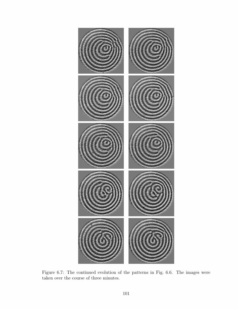
Figure 6.7: The continued evolution of the patterns in Fig. 6.6. The images weretaken over the course of three minutes.

101

Figure 6.8: Snapshots at ε = 0.60, showing sustained time-dependent patterns. Rel-ative to the pattern on the left, the center pattern is taken after 4th; the pattern atthe right is taken after 30th.

6.2 Pattern Forecasting

Armed with a model of the governing equations for a system, one is able to make

forecasts to future times, but first, one must use experimental measurements to de-

termine accurately an initial system state. A whole class of algorithms devised to

tackle this state estimation problem is based on variations of the Kalman filter. We

provide below some background and motivation for the development of the LETKF;

the reader is referred to Refs. [57, 60, 61, 62, 63] for historical and computational

details.

6.2.1 Kalman Filtering

Consider a system state denoted by the vector ξ, together with some model of the

governing equations M such that ξi+1 = M(ξi), where the index i is taken to refer to

a time step. It may be the case that measurements do not access the state variables

directly; rather, there is an observation mapping H such that one makes measure-

ments of H(ξ). Essentially, the task of the Kalman filter [64] is to find a trajectory

through phase space evolving according to the model equations which, when projected

into the observation space, best fits the time series of experimental measurements.

The Kalman filter (built on Bayesian inference) does this by using measurements to

evolve a Gaussian probability distribution around the best guess of the state; the

102

distribution is captured by a mean state and the covariance of deviations about that

state. This process is recursive; as more measurements are assimilated, the model

state eventually converges to the true state of the system, at which point forecasts

can be made by integrating the model state forward in time.

Extended Kalman Filter When the model M and the observation mapping

H are nonlinear, the probability distribution can no longer be expected to remain

Gaussian over time. However, if the nonlinearities are weak or measurements are

sufficiently frequent, it may work to linearize both the model and the observation

transform about the current state, regaining the original Kalman filter equations.

This additional step results in the so-called Extended Kalman Filter (EKF).

Ensemble Kalman Filter The computational limitation of the EKF is that,

at some point in the minimization of the cost function, there is a required inversion

of an N × N matrix, where N is the number of observation locations (which can

easily be of order 105 or more). The Ensemble Kalman Filter (EnKF) reduces the

dimension of state representation by using an ensemble of state vectors from which

a linear combination is formed to produce the best guess. The number of ensemble

members k must be large enough to account for the dynamical degrees of freedom

but, presumably, this will be smaller than N . In addition to reducing matrix sizes,

this formulation has the feature that each of the ensemble members evolves under the

full nonlinearity of M; effectively, the linearization exists in the approximation that

the actual state can be represented by a linear combination of nearby states.

6.2.2 LETKF

As the number of degrees of freedom increases, the necessary EnKF ensemble size

also grows and can reach a point where the computational bottleneck occurs in the

simulation of all ensemble members. Recent evidence suggests, for example, that

103

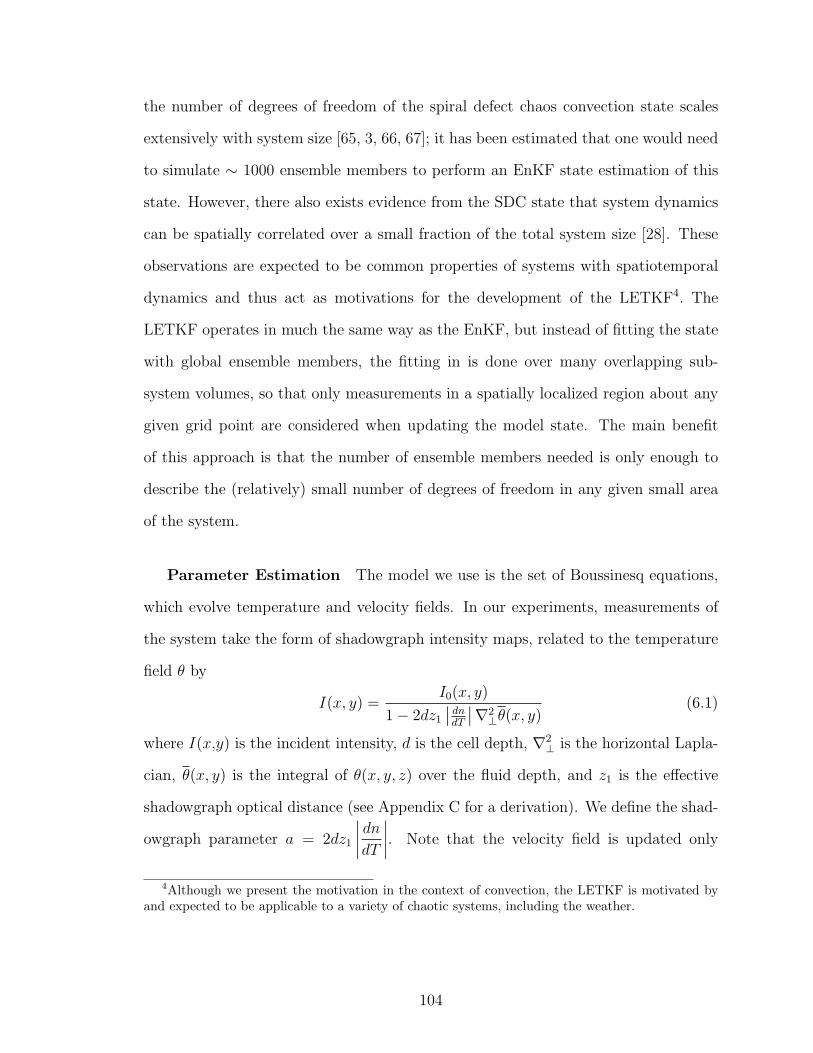
the number of degrees of freedom of the spiral defect chaos convection state scales

extensively with system size [65, 3, 66, 67]; it has been estimated that one would need

to simulate ∼ 1000 ensemble members to perform an EnKF state estimation of this

state. However, there also exists evidence from the SDC state that system dynamics

can be spatially correlated over a small fraction of the total system size [28]. These

observations are expected to be common properties of systems with spatiotemporal

dynamics and thus act as motivations for the development of the LETKF4. The

LETKF operates in much the same way as the EnKF, but instead of fitting the state

with global ensemble members, the fitting in is done over many overlapping sub-

system volumes, so that only measurements in a spatially localized region about any

given grid point are considered when updating the model state. The main benefit

of this approach is that the number of ensemble members needed is only enough to

describe the (relatively) small number of degrees of freedom in any given small area

of the system.

Parameter Estimation The model we use is the set of Boussinesq equations,

which evolve temperature and velocity fields. In our experiments, measurements of

the system take the form of shadowgraph intensity maps, related to the temperature

field θ by

I(x, y) =I0(x, y)

1− 2dz1

∣∣ dndT

∣∣∇2⊥θ(x, y)

(6.1)

where I(x,y) is the incident intensity, d is the cell depth, ∇2⊥ is the horizontal Lapla-

cian, θ(x, y) is the integral of θ(x, y, z) over the fluid depth, and z1 is the effective

shadowgraph optical distance (see Appendix C for a derivation). We define the shad-

owgraph parameter a = 2dz1

∣∣∣∣ dndT∣∣∣∣. Note that the velocity field is updated only

4Although we present the motivation in the context of convection, the LETKF is motivated byand expected to be applicable to a variety of chaotic systems, including the weather.

104

through its coupling to the temperature field inside the Boussinesq model. In addi-

tion to the temperature and velocity fields, the state estimation algorithm can also

be used to predict global variables such as this shadowgraph parameter a, as well as

the Prandtl and Rayleigh numbers. This is done by a simple extension of each state

vector to include a variable component for each global parameter being fit.

6.3 Preliminary Results

A time series of shadowgraph images, with ε = 0.60 are assimilated into the LETKF

at a rate of every tv/4 (2 Hz); the LETKF uses these measurements to update an

ensemble of model state vectors. Here we use k = 8 ensemble members. In be-

tween assimilation times, each ensemble state is integrated forward according to the

Boussinesq model. The best guess of the real state is formed by an average over the

ensemble.

To gauge convergence of the state, we attempt to fit the global Rayleigh number as

well as the shadowgraph parameter a and look at the spread of those parameter values

over the k ensemble states. In Fig. 6.9, we show the average Rayleigh number over the

ensemble, along with the standard deviation about the mean. The same information

is shown in Fig. 6.10 for a. Although the plots of deviations suggest that the state

has converged in just a few tv (consistent with earlier tests [57]), the behavior of the

average values suggests otherwise. The estimated values for the Rayleigh number

(∼ 2500) and a (-0.05) are, however, in the range of expected values. Note that the

estimated Rayleigh number is smaller than the true Rayleigh number (for ε = 0.60,

Ra = 2733); this was also observed in Ref. [57] and was attributed to the algorithm

implicitly accounting for possible model errors (non-Boussinesq effects) by using the

Rayleigh number that allows the times series of measurements to be best fit.

Because the measurement is in the form of shadowgraph images, the ultimate

comparison is of the actual shadowgraphs with those projected from the computed

105

0 10 20 30 40 50 60 70 80 902300

2400

2500

2600

2700

2800

2900

3000

3100

3200

Vertical diffusion times

Ens

embl

e av

erag

e, R

ayle

igh

num

ber

0 10 20 30 40 50 60 70 80 900.02

0.03

0.04

0.05

0.06

0.07

0.08

0.09

Vertical diffusion times

Sta

ndar

d de

viat

ion

over

ens

embl

e, R

A

Figure 6.9: On top, the average Rayleigh number of the ensemble, as shadowgraphsare assimilated; below, the standard deviation in the ensemble Rayleigh numbers,relative to the average Rayleigh number at that time.

106

0 10 20 30 40 50 60 70 80 90−0.06

−0.058

−0.056

−0.054

−0.052

−0.05

−0.048

Vertical diffusion times

Ens

embl

e av

erag

e, a

0 10 20 30 40 50 60 70 80 900.02

0.03

0.04

0.05

0.06

0.07

0.08

0.09

Vertical diffusion times

Sta

ndar

d de

viat

ion

over

ens

embl

e, a

Figure 6.10: On top, the average value of the shadowgraph parameter a over theensemble, as shadowgraphs are assimilated; below, the standard deviation in theensemble a values, relative to the average value at that time.

107

0 10 20 30 40 50 60 70 80 90800

900

1000

1100

1200

1300

1400

1500

1600

Length of data assimilation (in tv)

RM

S e

rror

Figure 6.11: The root mean square error between the predicted and observed shad-owgraph over assimilation (arbitrary units).

state. We define an rms (root mean square) error between the actual and predicted

shadowgraphs at each time step; this is plotted in Fig. 6.11. After the first few tv,

the error shows little behavior, also suggesting convergence at early times. A few of

the shadowgraphs are presented in Fig. 6.12. The best fit of the measurements by the

LETKF effectively allows the measurement noise to be filtered out. The predicted

shadowgraphs appear to differ from measurements most at times when the state is

undergoing instability (center pair of images), but the discrepancies disappear with

continued assimilation.

While these preliminary results are promising, there are several things undone.

The next step, experimentally, is to increase the level of control over the initial con-

ditions and develop an approach to creating a selected ensemble of patterns. While

the fast convergence of the model state is important, the ultimate goal is to produce

108

Figure 6.12: On the left are the actual shadowgraphs; on the right are those computedfrom the model state. These three images are taken at 30tv, 50tv, and 56tv (from topto bottom).

109

better forecasts. With that idea in mind, and with an ensemble of pattern evolutions

in hand, one can test the state estimation by comparing not only the convergence

across the experimental ensemble, but also the accuracy of forecasts.

110

CHAPTER VII

CONCLUSIONS

Rayleigh-Benard convection continues to be an extremely useful system for testing and

developing ideas about pattern formation and dynamics. The technique of pattern

actuation described herein takes advantage of the greenhouse effect of a commonly

used convective fluid, SF6, to provide the ability to repeatably create patterns exper-

imentally. This adds one more tool to already well-established methods for studying

the dynamics of convective patterns. Through pattern manipulation, we were able

to repeatably prepare straight roll patterns near secondary instabilities, and excite

the spatially localized dynamical modes by imposing selected perturbations to the

patterns. The distance from onset of a particular localized instability (the skew-

varicose) was quantified in terms by measured perturbation lifetimes. We extracted

the dominant spatial modes and their growth rates directly from the ensemble of

shadowgraph evolutions, at three locations in (q,ε) phase space; the modes were con-

cluded to be spatially localized versions of the global instabilities of infinite, ideal

systems. We extended the pattern imposition to non-periodic spatial patterns with a

circular boundary and showed preliminary results of estimating the fluid state (using

the LETKF) from these prepared patterns.

Our approach to extracting dynamical information by studying the evolutions

of many states with nearby initial conditions, although prevalent in theoretical and

numerical investigations, has been limited experimentally because of the difficulty in

preparing a state with a given set of initial conditions. We showed that, using an

experimentally created ensemble of nearby states, the dominant system modes can be

extracted directly from experimental measurements. The fact that the modes were

111

extracted without the use of a model set of governing equations suggests that the

approach could extend to systems where the governing equations are unknown or the

system geometry makes numerical modeling difficult. While pattern manipulation

through optical means is specific to our experiment, we expect the approach to be

applicable to a variety of systems, as long as an acceptable means of actuation can

be devised. Striking examples of candidate systems exist in biological tissue, where

control and prediction of the dynamics of voltage pulses in cardiac tissue or neurons

are major goals [68].

It would be an improvement to the current experiment to add the ability to ac-

tuate the convective flow from above. Specifically, it would be very interesting to see

if one would find any new dynamical response of straight roll patterns to perturba-

tive heating from above. Early actuation tests indicated that this type of heating

may suppress convection, as it effectively reduces the local temperature difference.

Selective heating of both boundaries would likely lead to an increased level of pattern

control, which would be helpful for studying more complex patterns.

Ultimately, a main goal is to extract dynamical modes systematically from a state

exhibiting chaotic or even fully turbulent behavior. One can imagine a back-and-forth

between using control to extract dynamical information and using that information

to enhance system control. The rich variety of dynamics observed in Rayleigh-Benard

convection suggests a natural extension of our approach to extracting experimentally

the dynamical modes of more complex convection states, such as spiral defect chaos,

where spatially localized instabilities occur in regions of locally parallel rolls. While

the global number of degrees of freedom may scale extensively with system size, it is

likely that the number of distinct modes is some fraction of that total; distant spatially

localized modes may be related in terms of translations, reflections, or rotations.

Just as we saw during modal extraction of the straight roll state, we can expect

considerations of symmetry to be useful in building a minimal description of the

112

important modes.

Chapter 6 lays the groundwork for further study into the prediction process. For

example, how much measurement information is needed for an accurate convergence

of a model state onto an experimental state near instability? Experimentally, the

next major step is to refine the process of preparing initial patterns, pushing the

limits of experimental repeatability of the initial conditions. The preliminary results

are promising, in that we did observe a high degree of reproducibility in the evolu-

tions of select imposed patterns. Because it is primarily through roll breakings and

connections that patterns rearrange, we may expect the state estimation process (and

thus prediction in general) to be sensitive to these instability events. Control over

the pattern differences would allow one to test the predictability in a systematic way.

It is worthwhile to note that both the modal extraction and the state estimation

procedure highlight an emerging way of thinking about the evolution of dynamical

systems by embedding observed states in a space spanned by a well-chosen basis [69].

In the case of weakly stable modes of straight rolls near instability, a good choice is a

basis formed from the slowly decaying structures; in state estimation, it is an evolving

ensemble of states in the neighborhood surrounding the estimated state. Embedding

system dynamics in a set of representative solutions is helpful by not only reducing

the dimensionality of representation but also by emphasizing that understanding of

the system evolution may simplify to understanding of special system solutions.

Together, accurate state estimation and knowledge of the system’s important dy-

namical modes would provide enormous possibility for system control. As suggested

in Ref. [54], the ability to control a nonlinear/chaotic system offers a significant ad-

vantage over a linear system. Namely, it is possible that a large variety of system

behavior can be achieved, for the purpose at hand, through the careful choice and

application of small changes to the system. Moreover, in systems where the important

modes tend to be spatially localized, it follows that changes in the global state may

113

be induced by the proper choice of actuation on a sub-region of the system.

114

APPENDIX A

GOVERNING EQUATIONS

A.1 Navier-Stokes

The fluid is governed by the Navier-Stokes equations as well as the heat equation.

This provides a set of three equations which describe, respectively, the movement of

mass, momentum, and heat through the fluid volume:

∂ρ

∂t+∇ · (ρu) = 0 (A.1)

ρ∂u

∂t+ ρ(u · ∇)u = −∇p+ µ∇2u (A.2)

∂T

∂t+ (u · ∇)T = κ∇2T (A.3)

The first continuity equation is simply the conservation of mass in differential

form which, for constant density, reduces to ∇ · u = 0. The second equation de-

scribes the conservation of momentum, and the third equation is a consequence of

the conservation of energy.

A.2 Uniform solution

We will analyze the RB system in which two horizontally infinite plates are fixed at

z = ±1

2d. The boundary conditions appropriate for experimental conditions are that

the temperatures at the top and bottom boundaries are fixed with ∆T = Tbot − Ttop

and vanishing velocity at the rigid boundaries. The uniform state that meets these

boundary conditions is a motionless state with a linear conducting profile

u = 0 (A.4)

Tcond = Tcond(z) = T − z

d∆T (A.5)

115

There will be small variation in the fluid density due to the temperature difference,

so we expand the density

ρ(T ) ≈ ρ(T0) +∂ρ

∂T(T − T0) = ρ0[1− α(T − T0)] (A.6)

where α = −1

ρ

∂ρ

∂Tis the coffecient of thermal expansion of the fluid. Note that while

the density fluctuations will ultimately give rise to a non-uniform state, the incom-

pressibility condition still holds reasonably well. That is, the velocity of the fluid will

be much less than the speed of sound. The assumption that we can ignore the varia-

tion of other fluid properties (thermal diffusivity, viscosity, etc.) with temperature is

known as the Oberbeck-Boussinesq approximation.

Substituting this state into the momentum equation, with the time-derivative set

to zero, gives an equation for the pressure

∂p

∂z= −ρ0g(1− α∆T

z

d) (A.7)

which can be integrated to give the steady pressure

pcond = p0 − ρ0g(z − α∆Tz2

2d) (A.8)

Note that p0 is an arbitrary choice since pressure only shows up in the Navier-Stokes

equations through a gradient.

A.3 Disturbances to Conduction State

We will introduce variables V, θ, and P for the disturbance fields of velocity, tem-

perature, and pressure, respectively.

v = V (A.9)

T = Tcond + θ (A.10)

p = pcond + P (A.11)

116

Substituting these expressions into the Boussinesq equations gives

∇ ·V = 0 (A.12)

∂V

∂t+ (V · ∇)V = −1

ρ∇p+ ν∇2V + αgθz (A.13)

∂θ

∂t+ (V · ∇)θ = κ∇2θ +

∆T

dVz (A.14)

A.4 Non-dimensionalization

In order to study the stability of the no-motion state, it is useful to first non-

dimensionalize the governing equations. We introduce scales for all variables:

t = τt′ (A.15)

r = dr′ (A.16)

V =d

τV′ (A.17)

θ = T0θ′ (A.18)

P = P0P′ (A.19)

We will substitute these equations terms but drop the primes for convenience.

From this point on, all variables will be dimensionless unless otherwise noted.

(d

τ 2)∂V

∂t+ (

d

τ 2)(V · ∇)V = −(P0)

1

ρ∇P + (

1

dτ)ν∇2V + (T0)αgθz (A.20)

(T0

τ)∂θ

∂t+ (

T0

τ)(V · ∇)θ = (

T0

d2)κ∇2θ + (

1

τ)∆TVz (A.21)

or,

∂V

∂t+ (V · ∇)V = −(

P0τ2

dρ)∇P + (

ντ

d2)∇2V + (

T0τ2αg

d)θz (A.22)

∂θ

∂t+ (V · ∇)θ = (

κτ

d2)∇2θ + (

1

T0

)∆TVz (A.23)

Let us choose τ =d2

κ, P0 =

dρ

τ 2, and T0 = κναgd3 which reduces the equations to

∂V

∂t+ (V · ∇)V = −∇P + (

ν

κ)(∇2V + θz) (A.24)

∂θ

∂t+ (V · ∇)θ = ∇2θ +

αg∆Td3

νκVz (A.25)

117

Here we can identify the two remaining non-dimensional parameters as the Prandtl

number Pr =ν

κand the Rayleigh number Ra =

αg∆Td3

νκ. The evolution equations

are typically written in the following form

∇ · u = 0 (A.26)

Pr−1(∂V

∂t+ (V · ∇)V) = −∇P +∇2V + θz (A.27)

∂θ

∂t+ (V · ∇)θ = ∇2θ +RaVz (A.28)

118

APPENDIX B

CAD DRAWINGS OF APPARATUS

Included in this chapter of the Appendix are the drawings for the parts comprising

the convection apparatus. See Chapter 2 for a schematic of the apparatus. The design

here is that the convection cell is sandwiched between two optical windows, each of

which is held in a metal plate: these plates are shown in Figs. B.1, B.2, B.3, and B.4.

Note that the top plate has four access ports, for connecting gas lines. Currently,

we use only one of these ports; the others are sealed. An O-ring placed between the

two plates forms the lateral pressure boundary (the optical windows form the vertical

boundaries); screws connect the plates. The heating and cooling chambers (Fig. B.5)

are identical, and screw into the top and bottom cell plates. An optical window on

each chamber seals against the circulating fluid; the windows are held in place by two

small metal plates (see Fig. B.6) which screw into the heating/cooling chambers.

119

Figure B.1: The top cell plate, part I.

120

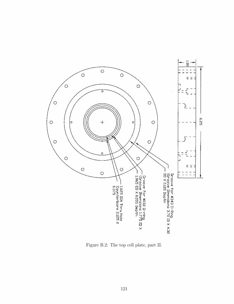
Figure B.2: The top cell plate, part II.

121

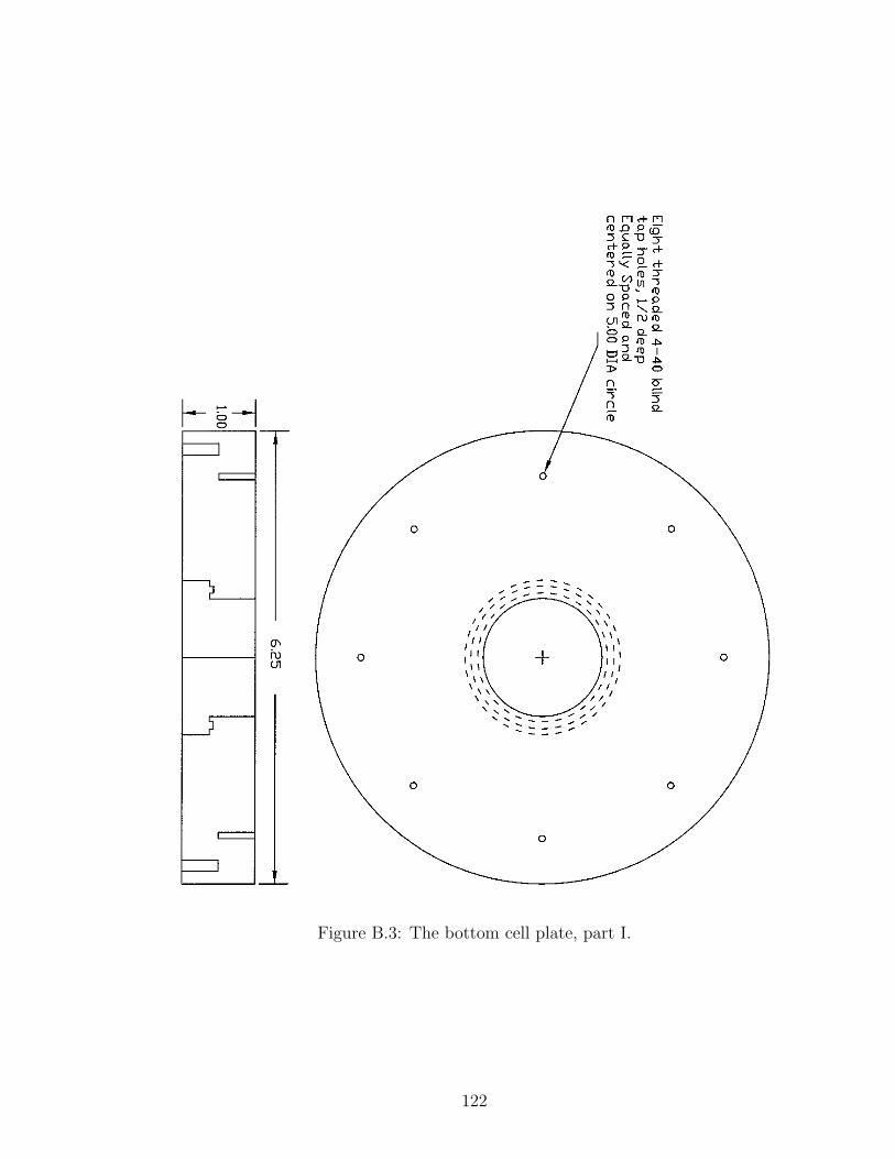
Figure B.3: The bottom cell plate, part I.

122

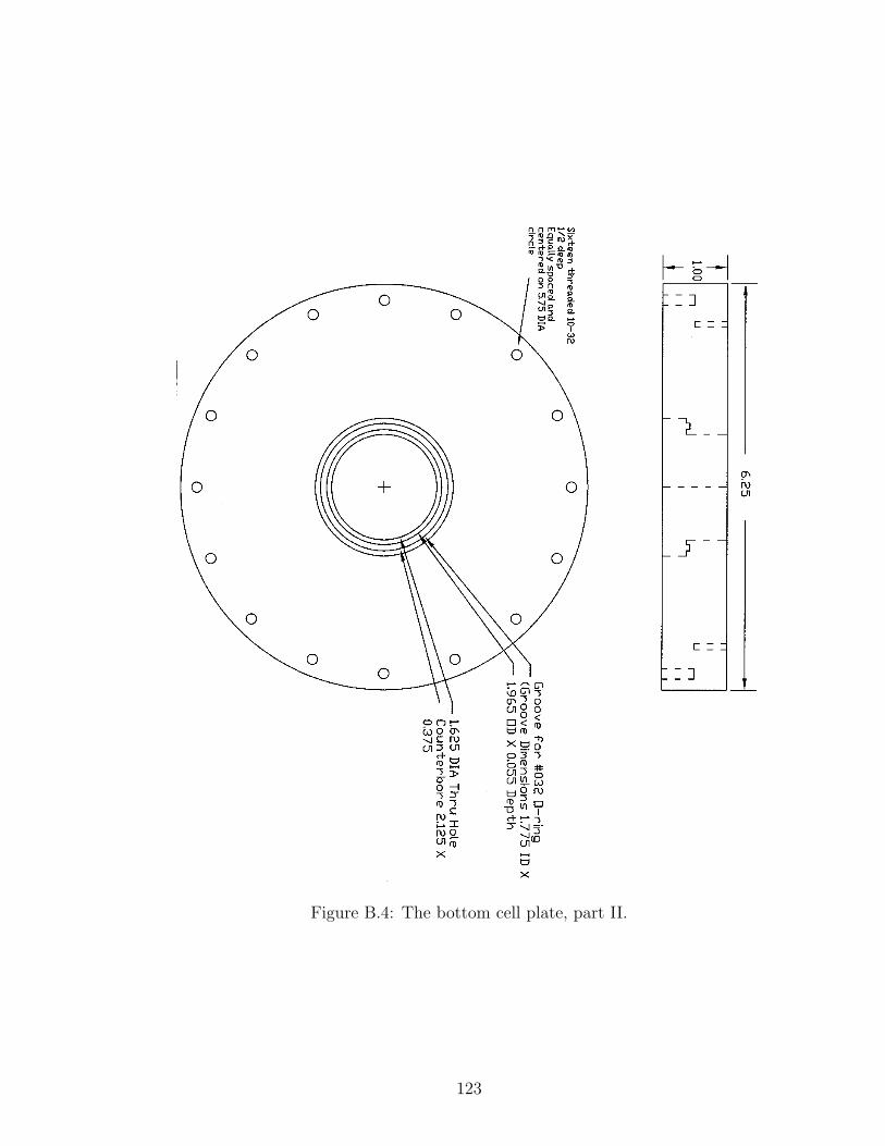
Figure B.4: The bottom cell plate, part II.

123

Figure B.5: The cooling (heating) chamber.

124

Figure B.6: The small plate used to hold the outer windows of the apparatus.

125

APPENDIX C

SHADOWGRAPH OPTICS

C.1 Geometric Optics

The following is a derivation of the relationship between the observed shadowgraph

intensity field and the convective temperature field, assuming a valid geometric optics

approximation. It follows Refs. [35, 36] and, most closely, Ref. [60].

The position of a ray of light r is expressed as a function of the path length s. The

ray path in a medium with inhomogenous refractive index n(x, y, z) is given by [70]

d

ds[n(r(s))

dr(s)

ds] = ∇n(r) (C.1)

The left-hand side can be expanded to

dn

ds

dr

ds+ n

d2r

ds2(C.2)

which we can re-write using

dn

ds=∂n

∂x

dx

ds+∂n

∂y

dy

ds+∂n

∂z

dz

ds= ∇n · dr

ds(C.3)

So we have

(∇n · drds

)dr

ds+ n

d2r

ds2= ∇n (C.4)

Let us define v ≡ dr

dsand rearrange to get

dv

ds=∇nn− (∇nn· v)v (C.5)

And here we notice that the right-hand side produces the projection of∇nn

onto the

plane perpendicular to v.

126

We will assume that the refractive index is a constant value with a small pertur-

bation field

n(x, y, z) = n0 + δn(x, y, z) (C.6)

where n0 is the refractive index evaluated at T of the fluid and from which follows

∇n(x, y, z)

n(x, y, z)≈ ∇δn(x, y, z) (C.7)

Because the refractive index variation is small, we can further assume the displace-

ment of the ray as it passes through the field is negligible but that it picks up a phase

that corresponds to a slight angular deflection. We are interested in the horizontal

components of the ray as it exits the fluid, so we choose v = z

dv

ds= ∇⊥δn (C.8)

where ∇⊥ denotes the ∇ operator in the horizontal coordinates x, y. Again, ignoring

deflections of the ray while in the fluid, we can integrate over the fluid depth to get

the overall phase shift of the ray as it exits the fluid:

v⊥ = 2d∇⊥δn (C.9)

The factor of 2 comes from traversing the fluid depth twice and dδn comes from the

integration and denotes the z-averaged value of the refractive index variation. This

expression gives the direction of the ray as it exits the fluid.

The final position of the ray is then given by

rf = r0 + z1z + 2dz1∇⊥δn (C.10)

a distance z1 >> d above the fluid.

Let us re-write this expression by defining

Hr0 = r0 + 2dz1∇⊥δn

n0r0

(C.11)

127

Then the Jacobian of this operator is

JH = 2dz1

1 +d2n

dx2

d2n

dxdyd2n

dxdy1 +

d2n

dy2

the determinant of which gives the change in the ray intensity at point rf . Expanding

this out and keeping only the leading order term in refractive index variation gives

|JH| = 1 + 2dz1∇2⊥δn(r0) (C.12)

and therefore the final light intensity is related to the incident intensity through

I(x, y) =I0(x, y)

1 + 2dz1∇2⊥δn(r0)

(C.13)

The refractive index is usually expressed conveniently in terms of the temperature

deviation θ

δn =dn

dTθ (C.14)

and becausedn

dTis negative in most cases, it is convenient to put the intensity rela-

tionship in the following final form

I(x, y) =I0(x, y)

1− 2dz1

∣∣ dndT

∣∣∇2⊥θ(x, y)

(C.15)

C.2 Physical Optics Corrections

In the geometric optics treatment, the deviations of light rays as they pass through

the fluid are not considered. Rather, it is the phase change, or angular deviation

of rays that give rise to a focusing effect of the rays in such a way as to reveal the

convection pattern. This treatment predicts certain optical distances at which the

strong focusing (the result of sharp dependence of refractive index on temperature,

for example) causes the shadowgraph intensity to diverge, which is clearly unphysical.

These locations are known as caustics. A more proper treatment of the shadowgraph

128

using physical optics is given in Ref. [36]. This section of the Appendix will review

the relevant results to our experimental setup.

Let us take as an illustration the simplified case of an ideal straight roll pattern.

The convection rolls act as cylindrical lenses and thus the authors define a geometric

focal length fgeo at which the first unphysical caustic appears. We can understand this

focal length from the expression above, in particular the term a = 2dz1

∣∣∣∣ dndT∣∣∣∣∇2⊥θ(x, y)

in the denominator. Geometric optics can be trusted quantitatively only in the limit

that this term is � 1.

Following the authors of Ref. [36], we consider, for simplicity, a straight roll pattern

defined by a single cosine term in the x-direction cos(qx), modulated by a single

sine term in the z-direction (to meet boundary conditions). The temperature term

∇2⊥θ(x, y) is estimated as ∼ 0.8q2∆T

√ε. We can then work backwards to find z1 =

a/(0.8q2

∣∣∣∣ dndT∣∣∣∣∆T√ε).

Let us take experimental conditions similar to our experiments: the depth d = 0.06

cm, mean temperature T = 24.0 deg C, pressure p = 215 psi, and ε = 1. We then find

∆Tc = 2.96 deg C, sodn

dT= −8.95 × 10−5/ deg C. Assuming a critical wavenumber,

q = 3.117/d = 52/cm, we find finally that fgeo, which occurs when a = 1, is equal

to 18 cm. However, from the LETKF algorithm, we have an estimate of a ≈ −0.06,

which tells us that z1 ≈ 2 cm. Thus z1/fgeo < 0.10 and we therefore conclude that

the magnitude of physical-optics corrections to the geometric treatment is relatively

small.

129

APPENDIX D

PROGRAM AND EXPERIMENT DETAILS

This chapter of the Appendix discusses some of the more technical and practical issues

that arise in running the experiment and using the LETKF state estimation program.

It is by no means an exhaustive description but is meant to address some of the less-

obvious details. The names of some programs, software, and special commands have

been set in italic text when appropriate, to distinguish them from idiomatic language.

Other function names and files have been set in single quotation marks.

D.1 The Experiment

D.1.1 The Computers

Two computers are used to run experiments. One computer (with Windows XP)

runs a Matlab program which analyzes shadowgraph images and makes calls to the

LaserShow program (call it computer #1) In parallel, computer #2 (with a Windows

2000 OS) runs the image-grabbing software (EPIX XCAP V2.2) and a Matlab pro-

gram that monitors and regulates temperatures of the top and bottom convection

cell boundaries. An ethernet cable connects the two computers so that images and

other files in shared folders can be accessed from either computer. The two folders are

stored in the ‘C:’ directory of computer #1 and can be accessed through ‘My Network

Places’ on the older computer. To avoid confusion, keep in mind that use of the older

computer (#2) is limited to setting the temperatures and initiating image taking (the

imaging software, which does not run on newer systems, is the reason for maintaining

this computer); most other mentions of function calls refer to using the newer com-

puter armed with the LS software and QM2000 board. Almost all the Matlab files

130

that are used can be found inside ‘C:\Matlab Functions’ on computer #1, except for

the temperature control files, which are in ‘E:\Matlab Functions’ on computer #2.

I have attempted to organize the files intuitively and have added comments to the

code that build on what is written here.

Software Backup The LS software exists on CD and has been shown to work

on both Windows XP and Windows 2000. The QM2000 board is a PCI board that

needs to moved to the same computer hosting the software. The XCAP software can

be downloaded from EPIX, but will not work without a parallel port dongle acting

as a Product Key (XCAP checks for this every time it is opened). The imaging

software will need to be updated for a newer OS. As of now, the XCAP software is

loaded on the other convection experiment computer (on Windows 2000) but would

need the Product Key to install the XCAP imaging board. In case of a computer #2

breakdown, the unused convection experiment computer could be used in its place.

Cell Assembly/Disassembly Changing the cell sidewalls requires planning.

First, the water in the top cooling chamber should be emptied and removed (keeping

the cell pressurized in the meantime, if possible). After de-pressurizing and opening

the convection cell, the bottom ZnSe should be removed, cleaned, and replaced quickly

(if at all; the ZnSe surfaces usually remain relatively clean), to minimize the amount

of CS2 that evaporates. Inevitably, there will be a pocket of air that gets trapped

below the ZnSe window. To get it out, the entire apparatus should be titled so that

the air leaves through one of the outlets. This is when one should be aware of putting

strain on the connecting tubes. As an aside—if one does not see a convection pattern

even with a large temperature difference between the top and bottom baths, consider

that there may be an air pocket keeping the CS2 from contacting the ZnSe boundary.

When the apparatus is disassembled, the O-rings and other parts should be

checked for signs of degradation, but the only parts that should need to be replaced

131

on a regular basis are the screws (it will usually be necessary to clean the interior of

the top cooling chamber; the aluminum is corroded by the water which causes small

flakes of material to build up). Note that the groove for the O-ring supporting the

ZnSe cell-bounding is for a size #032 O-ring, but we use a 1xx-series O-ring that fits

in the groove; this increases the contact area between the O-ring and window, which

prevents cracking of the AR-coating, up to ∼ 230 psi.

There are 16 screws (set evenly in a circle) that hold the top and bottom of the

convection apparatus together (see the CAD drawings). Tightening of these screws

compresses the laterally sealing O-ring and forces the top/bottom windows together.

Thus, it is important not to over-tighten, and to tighten evenly across the screws.

After the sidewalls have been placed between the windows and all other sealing parts

are in place, it makes sense to tighten the screws with under no pressure, to the

point that the sidewalls are pressed between the windows (they should not shift if

the entire apparatus is lifted/tilted). As the cell is pressurized, it is likely that the

windows will be pushed apart slightly, and the screws will have to be tightened to

re-trap the sidewalls between the windows (one will build an intuitive feel for how

much torque is needed, but one can actually notice visually when the sidewalls are

being compressed). When the sidewalls have been trapped between the windows at

the approximate pressure at which the experiments will be done, the screws can be

adjusted little by little until the two window surfaces forming the cell boundaries are

parallel (checked using laser interferometry). It is helpful in doing the assembly to

not attach the top cooling chamber until the alignment is done.

D.1.2 Setting Temperatures

Control of a water bath is activated by pressing a button on the back of the water

bath controllers labeled simply ‘ENABLE/DISABLE.’ A Matlab program, discussed

below, sets the temperature by sending a DC voltage via the Measurement Computing

132

DAQ; each miliVolt is a tenth of a degree Celsius. Two wires are used – one carries the

temperature-setting voltage, the other the ground voltage. The water bath manual

can be consulted for information about which pins can be used to access/control

settings.

Because the amount of RAM to run the imaging software and the Matlab tem-

perature control is significant, the older computer will slow down after some time,

so it may be necessary to restart the computer every few days of continual use (or

to set the priority of XCAP “above normal”). At a minimum, programs should be

shut down when not in use. Note, however, that control of the water baths should be

disabled when the computer restarts, or the bath will see a zero voltage and therefore

try to cool the water to 0◦ C.

The temperatures are measured using serial communication with the HP mul-

timeter (the multimeter should be set to receive signals from the back side). The

resistances of the thermistors are measured across pins in the back of the multimeter,

and a relay switch (activated by a 5 V signal from one of the DAQs) flips between

the top or the bottom thermistor. Incidentally, the pressure can be read from either

one of the DAQs (look at the wire connections) or from the multimeter, but it is not

possible under the current configuration to read both the resistances and the pressure

at the same time.

A Graphical User Interface ‘Exp Params GUI’ runs in Matlab and is the gateway

to measuring and changing temperatures. There are input fields for temperature set-

points, and there are three main functional buttons. The primary way to use this

interface is to set values for both top and bottom temperatures, and turn the program

to ‘ON.’ The feedback program will change the temperatures of the water baths via

changes in the voltages output . Pressing the ‘OFF’ button will turn off control

(naturally). There are two auxillary buttons that can be used to ‘fix’ the respective

temperatures. That is, changes are not allowed to the water bath temperature when

133

the respective temperature is ‘fixed.’ This is useful when control is wanted over only

one of the water baths. For example, it is best to leave the bottom temperature

near a set reference temperature. To do the mapping, the top temperature can be

increased quickly to bring ∆T below critical and then moved back afterward, all the

while leaving the bottom temperature unchanged. The GUI can also be used to get

temperature values without invoking control. This is initiated by pressing the ‘Just

Info’ button. Note that each day that temperature control is used, the set/measured

values are stored on computer #2 in a text file ‘C:\T Data\T data MM DD.txt’

where MM is the month and DD is the day.

D.1.3 Carbon Disulfide Considerations

Materials Use of CS2 as a heating fluid poses some challenges. An important

consideration is that, because it is a strong solvent, only select materials are appropri-

ate to use with CS2. Good materials include aluminum and Viton (and some similar

materials); the best place to check is the chemical compatibility checklist from Cole

Palmer, available online.

Sealing The relatively high vapor pressure means that it is difficult to entirely

seal the fluid as it flows through the heating loop. ‘Torr Seal’ epoxy has been used

around the joints connecting tubing to the pump, and Swagelok pieces are used at

other junctions. The possibility of a larger-scale spill is also a concern. For example, it

is necessary to pick up and/or tilt the convection apparatus from time to time, which

puts strain on the Swagelok-tubing connections; eventually, the tubing can wear down

and tear. One must remain aware of this whenever handling the apparatus. There

are multiple valves which can be shut to stop the flow. In the event of a spill, these

should be shut, the pump should be unplugged, an absorbent should be used to soak

up any spilled CS2 and keep it from evaporating into the lab. The plastic housing the

pump and tubing should be closed and time given for the CS2 to evaporate through

134

the vent.

Re-filling The continuous evaporation of CS2, however small, means that more

fluid will need to be added at some point (every 2-3 weeks, depending on how often

the experiment has been running). The pump should (obviously) be turned off to do

this. There is a small flap in the plastic surrounding the experiment, inside of which

is a cap that can be unscrewed to gain access to the fluid. Slowly, pour CS2 until it

starts approaching the level of the cap. Note that the evaporation may be minimized

by unplugging the pump whenever the experiment is not running.

D.1.4 Imaging

XCAP is on computer #2, which has a PCI board installed for communicating with

the digital camera (from the DVC company, model 1312). The graphical interface of

this program, from the EPIX company, makes it relatively straightforward to set the

frame rate, shutter rate, binning, etc.

During the mapping, XCAP should be set to record 5 ‘.tif’ images in the mapping

directory (‘C:\Mapping Images’), at a frame rate of 4 fps (‘Capture’ − > ‘Sequence

Capture’ − > ‘Video to Image Files’). The images should be named ‘mapping images’

to match the filename searched for by Matlab. Initialize XCAP to expect a ‘Script

Remote Control’ to be placed inside the mapping directory. XCAP scripts are basi-

cally pre-recorded steps that capture the user doing a series of tasks/manipulations

and can be useful when the same series of steps are used many times. This script

simply has recorded me pressing the ‘Record’ button on the image, and so, as the

mapping perturbation points are looped through, Matlab will repeatedly copy the

script into that folder, telling XCAP to begin taking images. Each time, XCAP will

take the 5 images (as it has been directed by the steps above) and then stop.

After mapping, images for analysis are placed in a different folder (‘C:\XCAP share’).

The maximum number of images and the frame rate can be set to the desired values.

135

The frame rate can slow when the number of images in the folder becomes large, so

it is sometimes appropriate to delete images as they are processed, if they will not be

needed later (see the Matlab function ‘get img’).

As far as the shadowgraph settings go, it is easiest to arrange the camera wher-

ever the best imaging can be realized. For some purposes, this will mean that the

magnification will be small and the roll intensities will be more “saturated”; for the

state estimation, it may be best to use a setting where the intensity maxima/minima

are not so pronounced, which would indicate that one is operating near the “z1 = 0

limit (see the shadowgraph discussion above), the limit that geometric optics is most

valid. The ultimate test is if the state estimation algorithm is able to converge onto

a shadowgraph parameter (see the state estimation details).

D.1.5 Mapping

Essentially, the mapping is a pair of matrices, each the size of the shadowgraph

images: ‘X fit’ and ‘Y fit’. At each element is the x (or y) value that corresponds

to that pixel value. Usually, a few individual mappings are done and the results are

averaged (and can be averaged with the already existing mapping). All the mapping

files are contained in ‘C:\Matlab Function\mappping’.

Before calling the mapping functions, the lateral boundaries of the convection

cell need to defined manually by four pixel coordinates. These are stored in the

‘Compute Mapping.m’ source file in textitglobal variables I and J . The 1 × 2 array

I holds the lowest and highest rows spanned by the convection cell, as viewed on

the shadowgraph images; likewise, J holds the lowest and highest columns. These

can be found simply by taking a background image and finding where the intensity

change indicates a cell boundary. Secondly, one must decide whether to recycle the

stored mapping or start afresh. Unless the cell or camera has shifted, the old mapping

is relevant. When the cell or camera has been shifted, however, it is important to

136

reset both I, J , and to compute an entirely new mapping. There are a few lines of

code within ‘Compute Mapping.m’ that should be commented out depending on if

the previous mapping is being used or not (these lines are marked).

The mapping code exists under several different .m files. The hierarchy is as

follows: The master file is ‘Do All Mapping(n),’ where n is the number of individual

mappings that are averaged together (n = 1 or 2 is sufficient if using the old mapping;

if starting over, use 3 or 4). Inside this function, the x and y values that are to be

perturbed serially are defined (these values may need to be changed if the sidewalls are

replaced or the cell shifts substantially). This function passes arrays of these values

to ‘Do Mapping Pts,’ which is the function that actually calls the LS software to

draw the points, copies the ‘mapping images.scr’ file into the proper folder (causing

XCAP to start imaging), and analyzes each shadowgraph image in order to find

the system response to the perturbation. After cycling through all points, what is

left is a set of (i,j) values, one pair for each (x,y) pair. These arrays are saved.

After returning to ‘Do All Mapping’, ‘Compute Mapping’ is called which opens these

saved points and sends them to ‘Filter Mapping Pts’, which filters out the spurious

data and does an iterative smoothing (as described in the main text). The resulting

maps ‘X fit’ and ‘Y fit’ are stored; ‘Compute Mapping’ reads these matrices and

either averages them with the old mapping or stores it averages only over the current

mapping iterations. Note that at this stage, the mapping exists as a set of global

variables and is stored in a ‘.mat’ file in ‘C:\Mapping Images\latest mapping’; call

the function ‘Reload Mapping’ to open this file and load the mapping variables (‘I’,

‘J’, ’X fit’, and ’Y fit’) back into the global workspace, if they have been cleared.

To convert between (i,j) and (x,y) once the mapping is complete, use ‘[x y] =

IJ to XY(i, j)’. For non-integer i or j values, the program simply interpolates using

the surrounding elements. Note that this is different from IJ to XY2, which does the

same thing, but uses only the initial planar fit (it is used for intermediate steps in

137

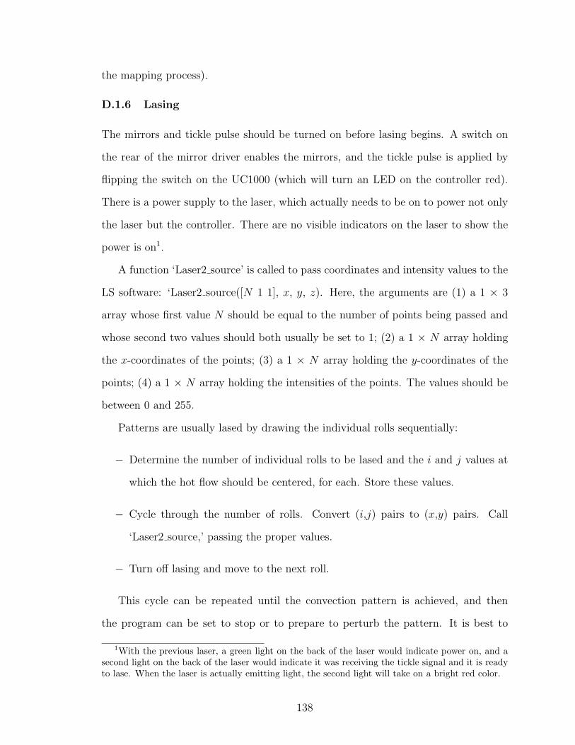
the mapping process).

D.1.6 Lasing

The mirrors and tickle pulse should be turned on before lasing begins. A switch on

the rear of the mirror driver enables the mirrors, and the tickle pulse is applied by

flipping the switch on the UC1000 (which will turn an LED on the controller red).

There is a power supply to the laser, which actually needs to be on to power not only

the laser but the controller. There are no visible indicators on the laser to show the

power is on1.

A function ‘Laser2 source’ is called to pass coordinates and intensity values to the

LS software: ‘Laser2 source([N 1 1], x, y, z). Here, the arguments are (1) a 1 × 3

array whose first value N should be equal to the number of points being passed and

whose second two values should both usually be set to 1; (2) a 1 × N array holding

the x-coordinates of the points; (3) a 1 × N array holding the y-coordinates of the

points; (4) a 1 × N array holding the intensities of the points. The values should be

between 0 and 255.

Patterns are usually lased by drawing the individual rolls sequentially:

− Determine the number of individual rolls to be lased and the i and j values at

which the hot flow should be centered, for each. Store these values.

− Cycle through the number of rolls. Convert (i,j) pairs to (x,y) pairs. Call

‘Laser2 source,’ passing the proper values.

− Turn off lasing and move to the next roll.

This cycle can be repeated until the convection pattern is achieved, and then

the program can be set to stop or to prepare to perturb the pattern. It is best to

1With the previous laser, a green light on the back of the laser would indicate power on, and asecond light on the back of the laser would indicate it was receiving the tickle signal and it is readyto lase. When the laser is actually emitting light, the second light will take on a bright red color.

138

build Matlab ‘m-files’ that run through these steps automatically, with some degree

of human intervention. See, for example, the ‘Target’ GUI, which has additional

function calls (see ‘get img.m’ and ‘lase out.m’, for example) and comments that

help to explain the process.

The effect of the laser can be enhanced by either increasing the intensity or by

adding ‘pause(t)’ statements after calling ‘Laser2 source’ in order to increase the

lasing time for any given roll, with t ∼ hundredths of ms. For a convection roll across

the cell domain, a few hundred points is usually appropriate. For a point perturbation,

pass on the order of 10 points that all have the same coordinates (sending only 1 point

will not cause a noticeable effect, presumably because of the rise/fall time of the laser).

Turning Off Laser It is best not to let the laser remain on unnecessarily, as it

can heat the glue holding the mirrors. In other words, the laser should be on only

when actively perturbing or imposing a pattern. To turn off the laser from within

Matlab (that is, rather than physically flipping switches), call ‘Laser2 source’ and

pass some x and y pair, such as (0,0), with zero brightness. In this case, also set

the second element of the first variable to 0; this acts as a backup to turn drawing

off: ‘Laser2 source([1,0,1], 0, 0, 0)’. Because the current laser does not have any

visible indicator if the laser is on or off, it is important to be sure to send this call

(or something equivalent) whenever done lasing.

‘Laser2 source’ The mirror rotations are controlled by the LaserShow Designer

2000 software package. There is a graphical interface (use the Desktop or the Start

Menu of Computer # 1), but, almost exclusively, we use one single function within

Matlab to communicate with the software. Note that the pattern coordinates (x,y)

should be set between the limits of ±8000.

The function ‘Laser2 source’ is a MEX-file. Changes must be made to the C++

source file and the project must be re-compiled. This can be done in Visual Studio,

139

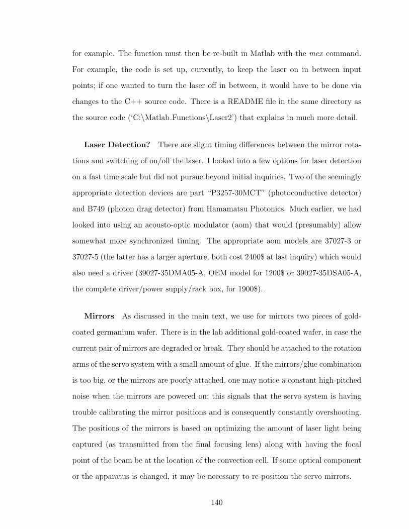
for example. The function must then be re-built in Matlab with the mex command.

For example, the code is set up, currently, to keep the laser on in between input

points; if one wanted to turn the laser off in between, it would have to be done via

changes to the C++ source code. There is a README file in the same directory as

the source code (‘C:\Matlab Functions\Laser2’) that explains in much more detail.

Laser Detection? There are slight timing differences between the mirror rota-

tions and switching of on/off the laser. I looked into a few options for laser detection

on a fast time scale but did not pursue beyond initial inquiries. Two of the seemingly

appropriate detection devices are part “P3257-30MCT” (photoconductive detector)

and B749 (photon drag detector) from Hamamatsu Photonics. Much earlier, we had

looked into using an acousto-optic modulator (aom) that would (presumably) allow

somewhat more synchronized timing. The appropriate aom models are 37027-3 or

37027-5 (the latter has a larger aperture, both cost 2400$ at last inquiry) which would

also need a driver (39027-35DMA05-A, OEM model for 1200$ or 39027-35DSA05-A,

the complete driver/power supply/rack box, for 1900$).

Mirrors As discussed in the main text, we use for mirrors two pieces of gold-

coated germanium wafer. There is in the lab additional gold-coated wafer, in case the

current pair of mirrors are degraded or break. They should be attached to the rotation

arms of the servo system with a small amount of glue. If the mirrors/glue combination

is too big, or the mirrors are poorly attached, one may notice a constant high-pitched

noise when the mirrors are powered on; this signals that the servo system is having

trouble calibrating the mirror positions and is consequently constantly overshooting.

The positions of the mirrors is based on optimizing the amount of laser light being

captured (as transmitted from the final focusing lens) along with having the focal

point of the beam be at the location of the convection cell. If some optical component

or the apparatus is changed, it may be necessary to re-position the servo mirrors.

140

D.1.7 Other Notes

− We purchased our ZnSe windows from Design Research Optics, and my main

contact there was the president, Bruce Sunderland. He can be reached by either

bruce@designresearchoptics.com or sales@designresearchoptics.com.

− For questions about the LS software, contact William Benner at Pangolin

(wrb@pangolin.com). He is the one who sent the Software Development Kit

that contained the Visual Basic and C++ source code for interacting with LS.

However, we have not been in contact for a few years.

− If the image frame rate seems to change during a time series of images, look at

the function ‘write file times.m’. This can be used to look at the time-stamps

of a given series of images; one can determine the “true” frame rate over the

time series, or one can compute shadowgraphs at the desired frame rate (by

interpolating between actual shadowgraphs).

− The critical temperature difference at a particular mean temperature and pres-

sure can be found by using the RBC.c program provided by G. Ahlers group.

This program exists on the computer used with the other convection experi-

ment. Open ‘Cygwin’ and change the directory to ‘G:\RBC Program.’ The

executable is named simply ‘RBC’ (invoke by ‘./RBC’). It is currently set to

take a mean temperature and pressure as arguments and to compute the ∆Tc,

given a particular cell depth, which can be changed by modifying ‘RBC.c.’ After

editing, run make to re-compile the code.

D.2 The LETKF Computer Code

The Boussinesq simulation is pieced together from code written during more than

one generation of Fortran (77 and 90). Two open-source Fortran compilers, gfortran

and g95, were used in attempts to compile the code, but neither was successful, the

141

reason being presumably the inability to process the older subroutines together with

the newer code into a single executable. Instead, we use a commercial compiler, Lahey

f95 (the same compiler as used by the Maryland group).

The simulation uses a pseudo-spectral method [71]. A backward Euler step is used

for linear terms and a second order Adams-Bashforth step for non-linear terms. The

fields are expressed in terms of Fourier components in phi and Chebyshev polynomials

in z.

D.2.1 Compiling

The simulation code consists of several separate files; a Makefile script containing

certain flags calls the compiler which then produces corresponding ‘.o’ object (binary)

files for all input Fortran files (it also makes an executable, but that can be ignored).

The Makefile can be invoked by the make command. The Makefile only needs to be

called whenever there has been a change to one of the simulation files.

Meanwhile, the state estimation code is contained in a set of C++ files. A script

called a link file calls the built-in gcc C++ compiler via a mpicc command to produce

the corresponding object files. Additionally, it makes accessible to the code (hence

the term link) a group of needed libraries (discussed below). With the simulation

object files already existing, the link file builds a single executable, currently named

‘kalman.’

There are a small number of necessary external libraries. One is known as the

FFTW (Fastest Fourier Transform in the West). A second set of libraries adds the

capability of parallel processing, using the protocol called MPICH2 ; these libraries

come from Argonne National Lab. The directory locations of these libraries of these

(and others, which are probably system-dependent) are present in the link file.

142

D.2.2 Header Files

The main C++ file is mpifekf.c. Under normal circumstances, this is the only file

containing source code which needs to be changed. Additionally, specific parameters

may need to be set within a small number of header files.

The input shadowgraph images need to be cropped and circular, leaving no back-

ground region apart from that in the corners of the resulting square. The images are

8-bit bitmap images; a Matlab program (‘tif to bmp’) is used to convert the images

from the original 12-bit intensities, crop the images, and write the final bitmap files.

Within the ‘def.h’ header file, the size of the input shadowgraphs needs to be set.

This number should be the number of pixels along one side of the square images.

Other parameters should be set inside the ‘parameters.h’ file, brief descriptions of

which are given in the following list; terms appearing in the file but not listed below

should not be changed.

− Radius The size of the cell radius in terms of the depth. This is the same as

the aspect ratio.

− Prandtl number Self-explanatory

− tdelh The time step of the simulation, in terms of the vertical diffusion time.

Note that the actual time step is twice this value.

− xdir if 1.0, Dirichlet boundary conditions, if 0, Neumman boundary conditions.

− Rayleigh number Self-explanatory

The number of grid points (PARAM NR in the radial direction, PARAM NT

in the θ direction, and PARAM NZ in the z-direction) can be set inside ‘dimen-

sions.h.’ Note that two points are added implicitly to PARAM NZ for the two

vertical boundaries. Some combinations may not work with the Fortran simulation

143

code, but it is uncommon to change these numbers. The current values work for

an aspect ratio of 20, but If the aspect ratio were to double, PARAM NR and

PARAM NT should roughly double; PARAM NZ can remain constant.

D.2.3 Main Program

The main file is ‘mpifekf.c. In addition to the main LETKF algorithm, there are many

smaller subroutines that can be used to make specific calculations (such as to create

an ensemble, open a field and simulate it forward in time, compute the vorticity,

etc.). By default these subroutines are simply commented out. At the beginning of

the function the following parameters are defined.

DATA FILE The first of two output files containing information about the

parameter estimates, e-dimension, and other useful data/parameters.

RMS FILE One of the ‘.dat files written. The rms error between predicted and

actual shadowgraphs is written to the file and can be monitored; convergence

of this error can be used to monitor convergence to a state.

MEASUREMENT BASE This is the directory containing the shadowgraph

images. Be sure to include the correct number of zeros, such that the indexing

goes like 001, 002... as opposed to 1, 2,

OUTPUT DIR The path to the folder where ensemble members and esti-

mated shadowgraphs are put.

INIT ENSEMBLE The path to a set of random states used to initialize the

ensemble.

OPEN INITIAL Set to 1 to open the initial ensemble. This is the usual case,

unless creating a new ensemble with a new aspect ratio, for example, in which

case set to 0.

144

ANA ENSEMBLE SAVE Rate at which to save analysis ensemble members

(as ‘.vtk’ files). Looking at the ensemble is useful for debugging.

BG ENSEMBLE SAVE Rate at which to save the background ensemble

members (as ‘.vtk’ files).

RA Either the actual value, or the mean of an initial guess of the Rayleigh

number.

PR The Prandtl number.

MEANH1 The initial guess of H1, the parameter in the shadowgraph obser-

vation operator.

SEED The seed for the random number generator.

MAXSIM The maximum number of frames to assimilate.

DFRAME The frequency of frames to assimilate. For example, when set to

1, every frame is used, when set to 2, every other frame is used, and so on.

INIT FRAME The initial frame number.

T The amount of time (in terms of the vertical diffusion time) between assim-

ilated frames. This should usually be set to some multiple of DFRAME. For ex-

ample, if the time between shadowgraphs is tv/8, then set this to (1/8)(1/2tdelh),

where tdelh is set in ‘parameters.h’.

NEUMAN This is set to 0 and means that the simulation is using conducting

boundary conditions.

K The number of ensemble members.

S The number of observations within a disk. To use all pixels, set to SGN*SGN;

to use half, set to SGN*SGN/2, etc.

145

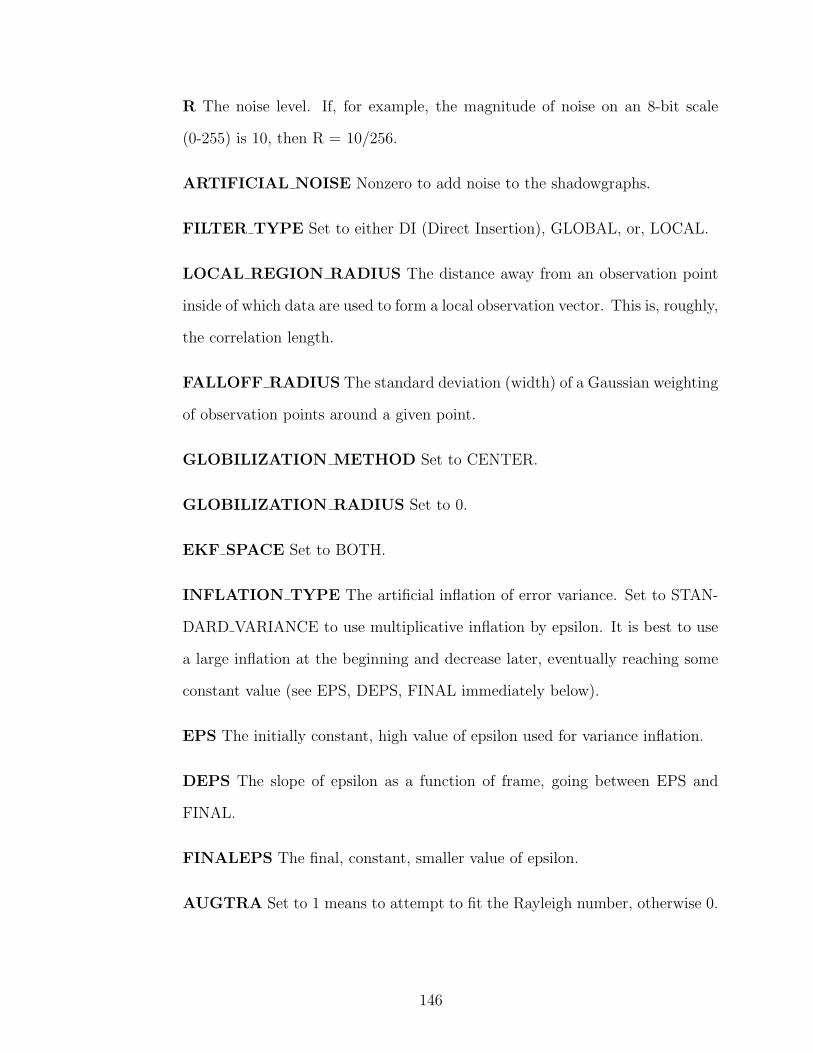
R The noise level. If, for example, the magnitude of noise on an 8-bit scale

(0-255) is 10, then R = 10/256.

ARTIFICIAL NOISE Nonzero to add noise to the shadowgraphs.

FILTER TYPE Set to either DI (Direct Insertion), GLOBAL, or, LOCAL.

LOCAL REGION RADIUS The distance away from an observation point

inside of which data are used to form a local observation vector. This is, roughly,

the correlation length.

FALLOFF RADIUS The standard deviation (width) of a Gaussian weighting

of observation points around a given point.

GLOBILIZATION METHOD Set to CENTER.

GLOBILIZATION RADIUS Set to 0.

EKF SPACE Set to BOTH.

INFLATION TYPE The artificial inflation of error variance. Set to STAN-

DARD VARIANCE to use multiplicative inflation by epsilon. It is best to use

a large inflation at the beginning and decrease later, eventually reaching some

constant value (see EPS, DEPS, FINAL immediately below).

EPS The initially constant, high value of epsilon used for variance inflation.

DEPS The slope of epsilon as a function of frame, going between EPS and

FINAL.

FINALEPS The final, constant, smaller value of epsilon.

AUGTRA Set to 1 means to attempt to fit the Rayleigh number, otherwise 0.

146

AUGTPR Same as above, but for Prandtl number. Leave set to 0 because of

computational expense of fitting.

AUGTH1 Same as above, but for H1, the parameter in the shadowgraph

observation operator.

RA SPREAD The initial spread .

PR SPREAD Same as above, but for Prandtl number. Leave set to 0 because

of computational expense of fitting.

SVDH1 Same as two terms above, but for H1.

PARAM SPREAD START Set to 0.

D.2.4 Other Comments and Considerations

− An assimilation rate of roughly four Hz works well.

− The program outputs ‘.vtk’ files from time to time. These files contain system

states in the form of grid locations with temperature and velocity values. They

can be visualized in Paraview, an open-source program.

− In addition to the rms error and the esimated state parameters, convergence of

the e-dimension is a way to check convergence onto a state. It falls between one

and (K-1) and represents the dimension of the ensemble members (see Ref. [72]).

− The maximum aspect ratio that has been used is 20. The time for the simulation

scales as Γ2ln(Γ).

147

REFERENCES

[1] F. H. Busse and J. A. Whitehead, “Instabilities of convection rolls in a highPrandtl number fluid,” J. Fluid Mech., vol. 47, pp. 305–320, 1971.

[2] S. W. Morris, E. Bodenschatz, D. S. Cannel, and G. Ahlers, “Spiral defect chaosin large aspect ratio Rayleigh-Benard convection,” Phys. Rev. Lett., vol. 71,pp. 2026–2029, 1993.

[3] D. A. Egolf, I. V. Melnikov, W. Pesch, and R. E. Ecke, “Mechanism of extensivespatiotemporal chaos in Rayleigh-Benard convection,” Nature, vol. 404, pp. 733–736, 2000.

[4] V. Croquette, “Convective pattern dynamics at low Prandtl number: Part II,”Contemp. Phys., vol. 30, pp. 153–171, 1989.

[5] M. C. Cross and P. C. Hohenberg, “Pattern formation outside of equilibrium,”Rev. Mod. Phys., vol. 65, p. 851, 1993.

[6] M. Cross and H. Greenside, Pattern formation and dynamics in non-equilibriumsystems. Cambridge University Press, 2009.

[7] J. P. Gollub and J. S. Langer, “Pattern formation in nonequilibrium physics,”Rev. Mod. Phys., vol. 71, pp. S396–S403, 1999.

[8] A. C. Newell, T. Passot, and J. Lega, “Order parameter equations for patterns,”Ann. Rev. Fluid Mech., vol. 25, pp. 399–453, 1993.

[9] H. Benard, “Les tourbillons cellulaires dans une nappe liquide,” Rev. Gen. Sci.Pure Appl., vol. 11, p. 1309, 1900.

[10] H. Benard, “Les tourbillons cellulaires dans une nappe liquide transportant de lachaleur par convection en regime permanent,” Ann. Chim. Phys., vol. 23, p. 62,1901.

[11] L. Rayliegh, “On convection currents in a horizontal layer of fluid, when thehigher temperature is on the under side,” Phil. Mag., vol. 32, p. 529, 1916.

[12] H. Jeffreys, “The stability of a layer of fluid heated below,” Phil. Mag., vol. 2,p. 833, 1926.

[13] H. Jeffreys, “Some cases of instability in fluid motion,” Proc. Roy. Soc. A,vol. 118, p. 195, 1928.

[14] J. Boussinesq, Theorie Analytique de la Chaleur, Vol. 2. Gauthier-Villars, 1903.

148

[15] A. Oberbeck, “Uber die warmeleitung der flussigkeiten bei der berucksichtigungder stromungen infolge von temperaturdifferenzen,” Ann. Phys. Chem., vol. 7,pp. 271–292, 1879.

[16] S. Chandrasekhar, Hydrodynamic and Hydromagnetic Stability. Oxford Univer-sity Press, 1961.

[17] E. Bodenschatz, W. Pesch, and G. Ahlers, “Recent developments in Rayleigh-Benard convection,” Ann. Rev. Fluid Mech., vol. 32, pp. 1340–778, 2000.

[18] H. Kurtuldu, K. Mischaikow, and M. F. Schatz, “Measuring the departures fromthe Boussinesq approximation in Rayleigh-Benard convection experiments,” J.Fluid Mech., 2011 (Accepted).

[19] G. Ahlers, F. F. Araujo, D. Funfschilling, S. Grossman, and D. Lohse, “Non-Oberbeck-Boussinesq effects in gaseous Rayleigh-Benard convection,” Phys. Rev.Lett., vol. 98, p. 054501, 2007.

[20] A. Schluter, D. Lortz, and F. H. Busse, “On the stability of steady finite ampli-tude convection,” J. Fluid Mech., vol. 23, pp. 129–144, 1965.

[21] R. M. Clever and F. H. Busse, “Transition to time-dependent convection,” J.Fluid Mech., vol. 65, pp. 625–645, 1974.

[22] F. H. Busse and R. M. Clever, “Instabilities of convection rolls in a fluid ofmoderate Prandtl number,” J. Fluid Mech., vol. 91, pp. 319–335, 1979.

[23] F. H. Busse, “The oscillatory instability of convection rolls in a low Prandtlnumber fluid,” J. Fluid Mech., vol. 52, pp. 97–112, 1972.

[24] E. D. Siggia and A. Zippelius, “Pattern selection in Rayleigh-Benard convectionnear threshold,” Phys. Rev. Lett., vol. 47, pp. 835–838, 1981.

[25] M. C. Cross, “Phase dynamics of convective rolls,” Phys. Rev. A, vol. 27, pp. 490–498, 1983.

[26] K.-H. Chiam, M. R. Paul, M. C. Cross, and H. S. Greenside, “Mean flow and spi-ral defect chaos in Rayleigh-Benard convection,” Phys. Rev. E, vol. 67, p. 056206,2003.

[27] R. V. Cakmur, D. A. Egolf, B. B. Plapp, and E. Bodenschatz, “Bistability andcompetition of spatiotemporal chaotic and fixed point attractors in Rayleigh-Benard convection,” Phys. Rev. Lett., vol. 79, p. 1853, 1997.

[28] S. W. Morris, E. Bodenschatz, D. S. Cannell, and G. Ahlers, “The spatiotemporalstructure of spiral-defect chaos,” Physica D, vol. 97, p. 164, 1996.

[29] R. E. Ecke, Y. Hu, R. Mainieri, and G. Ahlers, “Excitation of spirals and chiralsymmetry breaking in Rayleigh-Benard convection,” Science, vol. 269, pp. 1704–1707, 1995.

149

[30] E. N. Lorenz, “Deterministic nonperiodic flow,” Journal of Atmospheric Sci-ences, vol. 20, pp. 130–141, 1963.

[31] V. Croquette, “Convective pattern dynamics at low Prandtl number: Part I,”Contemp. Phys., vol. 30, pp. 113–133, 1989.

[32] J. R. de Bruyn, E. Bodenschatz, S. W. Morris, S. P. Trainoff, Y. Hu, D. S.Cannell, and G. Ahlers, “Apparatus for the study of Rayleigh-Benard convectionin gases under pressure,” Rev. Sci. Instrum., vol. 67, p. 2043, 1996.

[33] J. S. Steinhart and S. R. Hart, “Calibration curves for thermistors,” Deep SeaResearch and Oceanographic Abstracts, vol. 15, pp. 497–503, 1968.

[34] G. S. Settles, Schlieren and shadowgraph techniques: visualizing phenomena intransparent media. Springer, 2001.

[35] S. Rasenat, G. Hartung, B. L. Winkler, and I. Rehberg, “The shadowgraphmethod in convection experiments,” Experiments in Fluids, vol. 7, pp. 412–420,1989.

[36] S. P. Trainoff and D. S. Cannell, “Physical optics treatment of the shadowgraph,”Phys. Fluids, vol. 14, pp. 1340–1363, 2002.

[37] J. Tang and H. H. Bau, “Stabilization of the no-motion state in Rayleigh-Benard convection through the use of feedback control,” Phys. Rev. Lett., vol. 70,pp. 1795–1798, 1993.

[38] L. E. Howle, “Active control of Rayleigh-Benard convection,” Phys. Fluids, vol. 9,pp. 1861–1863, 1997.

[39] A. C. Or, L. Cortelezzi, and J. L. Speyer, “Robust feedback control of Rayleigh-Benard convection,” J. Fluid Mech., vol. 437, pp. 175–202, 2001.

[40] J. A. Domaradzki, “Heat transfer enhancement in Rayleigh-Benard convection,”Int. J. Heat Mass Transfer, vol. 32, pp. 2475–2483, 1989.

[41] M. M. Chen and J. A. Whitehead, “Evolution of two-dimensional periodicrayleigh convection cells of arbitrary wave-numbers,” J. Fluid Mech., vol. 31,p. 1, 1968.

[42] J. A. Whitehead, “Dislocations in convection and the onset of chaos,” Phys.Fluids, vol. 26, pp. 2899–2904, 1983.

[43] J. A. Whitehead, “The propagation of dislocations in Rayleigh-Benard rolls andbimodal flow,” J. Fluid Mech., vol. 75, pp. 715–720, 1976.

[44] D. Semwogerere and M. F. Schatz, “Evolution of hexagonal patterns from con-trolled initial conditions in a Benard-Marangoni convection experiment,” Phys.Rev. Lett., vol. 88, p. 054501, 2002.

150

[45] J. D. Anderson, Jr., “Computations of co2 laser radiation absorption in sf6-airboundary layers,” AIAA J., vol. 12, pp. 1527–1533, 1974.

[46] J. D. Anderson, Jr., J. L. Wagner, and J. Knott, “Co2 laser radiation absorptionin sf6,” AIAA J., vol. 11, pp. 1424–1426, 1973.

[47] M. S. Heutmaker and J. P. Gollub, “Wave-vector field of convective flow pat-terns,” Phys. Rev. A, vol. 35, p. 242, 1987.

[48] C. Normand, Y. Pomeau, and M. G. Velarde, “Convective instability: A physi-cist’s approach,” Rev. Mod. Phys., vol. 49, pp. 581–624, 1977.

[49] D. A. Egolf, I. V. Melnikov, and E. Bodenschatz, “Importance of local patternproperties in spiral defect chaos,” Phys. Rev. Lett, vol. 80, pp. 3228–3231, 1998.

[50] L. Sirovich, “Turbulence and the dynamics of coherent structures: Part i-iii,” Q.Appl. Math., vol. 45, p. 561, 1987.

[51] A. E. Deane and L. Sirovich, “A computational study of Rayleigh-Benard convec-tion. part 1. rayleigh number dependence,” J. Fluid Mech., vol. 222, pp. 231–250,1991.

[52] M. Ilaka and C. W. Rowley, “Modeling of transitional channel flow using balancedproper orthogonal decomposition,” Phys. Fluids, vol. 20, p. 034103, 2008.

[53] Y. Hidaka and S. Kai, “Nambu-goldstone mode and spatiotemporal chaos,”Forma, vol. 24, pp. 123–125, 2009.

[54] E. Ott, C. Grebogi, and J. A. Yorke Phys. Rev. Lett., vol. 64, p. 1196, 1990.

[55] M. R. Paul, K. H. Chiam, M. C. Cross, P. F. Fischer, and H. S. Greenside, “Pat-tern formation and dynamics in Rayleigh-Benard convection: numerical simula-tions of experimentally realistic geometries,” Physica D, vol. 184, pp. 114 – 126,2003.

[56] W. Decker, W. Pesch, and A. Weber, “Spiral defect chaos in Rayleigh-Benardconvection,” Phys. Rev. Lett., vol. 73, pp. 648–651, 1994.

[57] M. Cornick, B. Hunt, E. Ott, H. Kurtuldu, and M. F. Schatz, “State and param-eter estimation of spatiotemporally chaotic systems illustrated by an applicationto Rayleigh-Benard convection,” Chaos, vol. 19, p. 013108, 2009.

[58] B. B. Plapp, D. A. Egolf, E. Bodenschatz, and W. Pesch, “Dynamics and selec-tion of giant spirals in Rayleigh-Benard convection,” Phys. Rev. Lett., vol. 81,pp. 5334–5337, 1998.

[59] B. B. Plapp, Spiral pattern formation in Rayleigh-Benard convection. PhD thesis,Cornell University, 1997.

151

[60] M. Cornick, Problems in spatiotemporal chaos. PhD thesis, University of Mary-land, 2007.

[61] E. Ott, B. R. Hunt, I. Szunyogh, A. V. Zimin, E. J. Kostelich, M. Corazza,E. Kalnay, D. J. Patil, , and J. A. Yorke, “A local ensemble Kalman filter foratmospheric data assimilation,” Tellus, Ser. A, vol. 56, p. 415, 2004.

[62] E. Ott, B. R. Hunt, I. Szunyogh, A. V. Zimin, E. J. Kostelich, M. Corazza,E. Kalnay, D. J. Patil, , and J. A. Yorke, “Estimating the state of large spatio-temporally chaotic systems,” Phys. Lett. A, vol. 330, p. 365, 2004.

[63] B. R. Hunt, , E. J. Kostelich, and I. Szunyogh, “Efficient data assimilation forspatiotemporal chaos: A local ensemble transform Kalman filter,” Physica D,vol. 230, p. 112, 2007.

[64] R. Kalman, “A new approach to linear filtering and prediction problems,” J.Basic Eng., vol. 82, pp. 35–45, 1960.

[65] S. M. Zoldi, J. Liu, K. M. S. Bajaj, H. S. Greenside, and G. Ahlers, “Extensivescaling and nonuniformity of the Karhunen-Loeve decomposition for the spiral-defect chaos state,” Phys. Rev. E, vol. 58, pp. R6903–R6906, 1998.

[66] M. R. Paul, M. I. Einarsson, P. F. Fischer, and M. C. Cross Phys. Rev. E, vol. 75,p. 045203, 2007.

[67] H. Kurtuldu, K. Mischaikow, and M. F. Schatz, “Extensive scaling from com-putational homology and Karhunen-Loeve decomposition analysis of Rayleigh-Benard convection experiments,” Phys. Rev. Lett., 2011 (Accepted).

[68] W. Rappel, F. Fenton, and A. Karma, “Spatiotemporal control of wave instabil-ities in cardiac tissue,” Phys. Rev. Lett., vol. 83, pp. 456–459, 1999.

[69] J. F. Gibson, J. Halcrow, and P. Cvitanovic, “Visualizing the geometry of statespace in plane Couette flow,” J. Fluid Mech., vol. 611, pp. 107–130, 2008.

[70] M. Born and E. Wolf, Principles of optics. Cambridge University Press, sev-enth ed., 2003.

[71] L. S. Tuckerman, “Divergence-free velocity fields in nonperiodic geometries,” J.Comput. Phys., vol. 80, pp. 403–441, 1989.

[72] M. Oczkowski, I. Szunyogh, and D. J. Patil, “Mechanisms for the development oflocally low-dimensional atmospheric dynamics,” J. Atmos. Sci, vol. 62, pp. 1135–1156, 2005.

152

VITA

Adam C. Perkins was born in Des Moines, Iowa in 1983 and grew up in Waterloo,

Iowa. After graduating from the University of Northern Iowa with a B. S. in Physics

and minor in Mathematics, Adam joined the School of Physics at Georgia Tech in

August 2005.

153