medical imaging and virtual medicine - ggg
TRANSCRIPT
1
Dirk Bartz, Visual Computing for [email protected]
Lecture 2:
Histograms, Classification,Segmentation
Medical Imaging and Virtual Medicine
[email protected] 2005
Literature (1)
Paper:• G. Kindlmann, D. Durkin: Semi-Automatic Generation of
Transfer Functions for Direct Volume Rendering, Proc. IEEE Symposium on Volume Visualization, 1998.
• V. Pekar, R. Wiemker, D. Hempel: Fast Detection of Meaningful Isosurfaces for Volume Data Visualization, IEEE Visualization, 2001.
• J. Kniss, G. Kindlmann, C. Hansen: Interactive Volume Rendering Using Multi-Dimensional Transfer Functions and Direct Manipulation Widgets, IEEE Visualization, 2001.

2
[email protected] 2005
Outline
Histograms and Classification
Windowing
Histogram Filter
Segmentation
[email protected] 2005
Histogram and Classification (1)
• Recall:Volume Data are typically 8-12bit deep
• Value distribution of voxels of dataset is called histogram:• With 8bit: value distribution of 256
possible data values• With 12bit: 4096 possible data values

3
[email protected] 2005
Histogram and Classification (2)
MRI Dataset, T2 weighted (fluids)
Linear histogram
[email protected] 2005
Histogram and Classification (3)
Logarithmic histogram
MRI Dataset, T2 weighted (fluid)
(filtered brighter)
4
[email protected] 2005
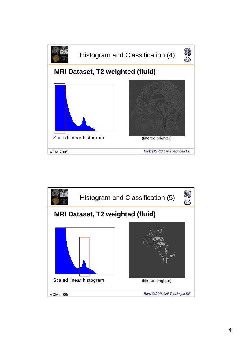
Histogram and Classification (4)
MRI Dataset, T2 weighted (fluid)
Scaled linear histogram (filtered brighter)
[email protected] 2005
Histogram and Classification (5)
MRI Dataset, T2 weighted (fluid)
Scaled linear histogram (filtered brighter)
5
[email protected] 2005
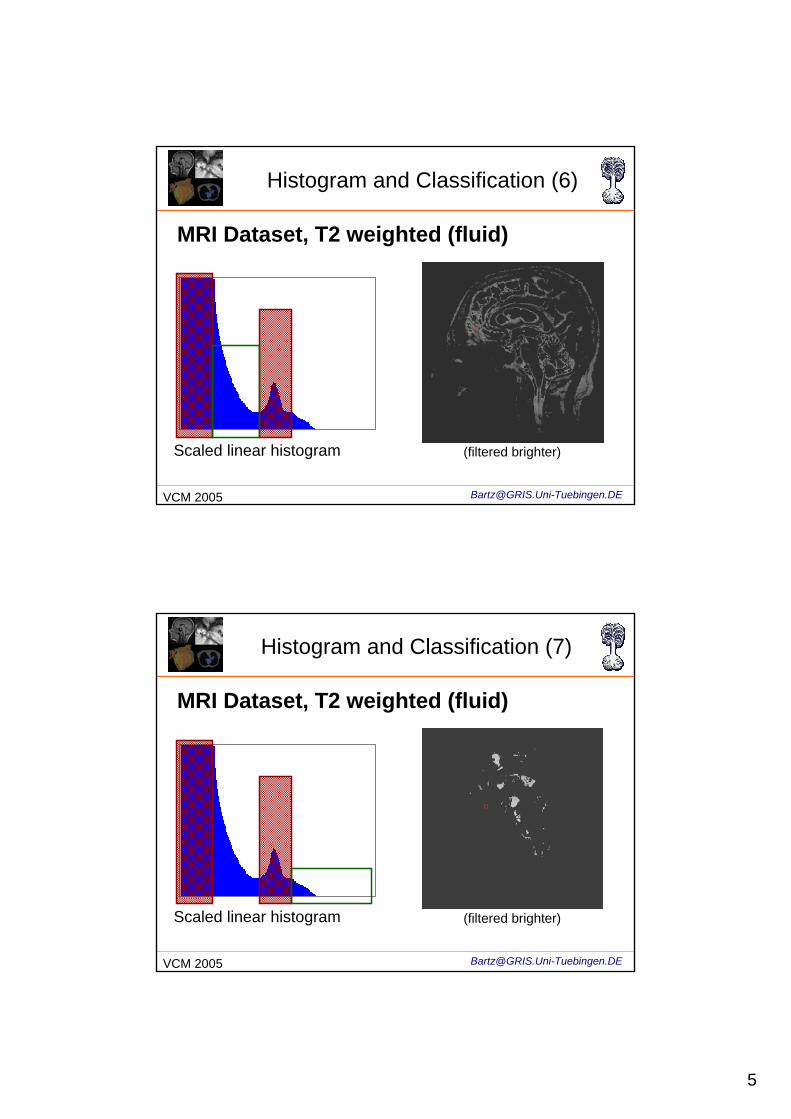
Histogram and Classification (6)
MRI Dataset, T2 weighted (fluid)
Scaled linear histogram (filtered brighter)
[email protected] 2005
Histogram and Classification (7)
MRI Dataset, T2 weighted (fluid)
Scaled linear histogram (filtered brighter)
6
[email protected] 2005
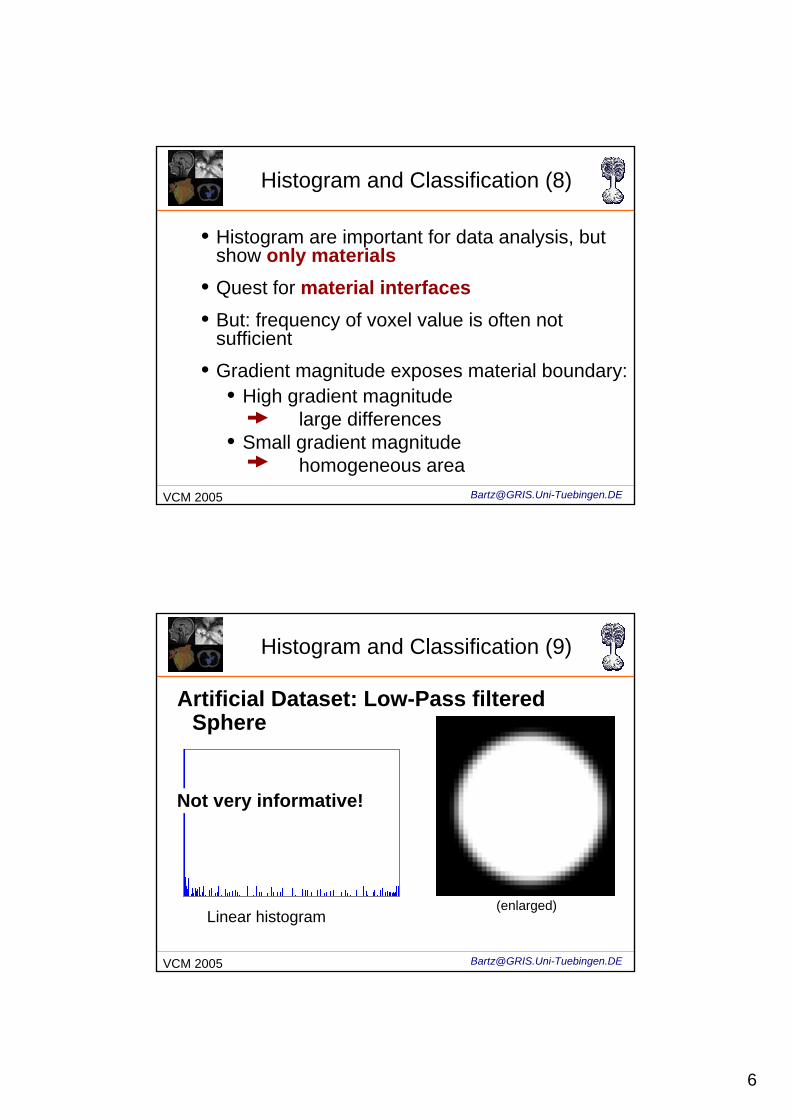
Histogram and Classification (8)
• Histogram are important for data analysis, but show only materials
• Quest for material interfaces• But: frequency of voxel value is often not
sufficient
• Gradient magnitude exposes material boundary:• High gradient magnitude
large differences• Small gradient magnitude
homogeneous area
[email protected] 2005
Histogram and Classification (9)
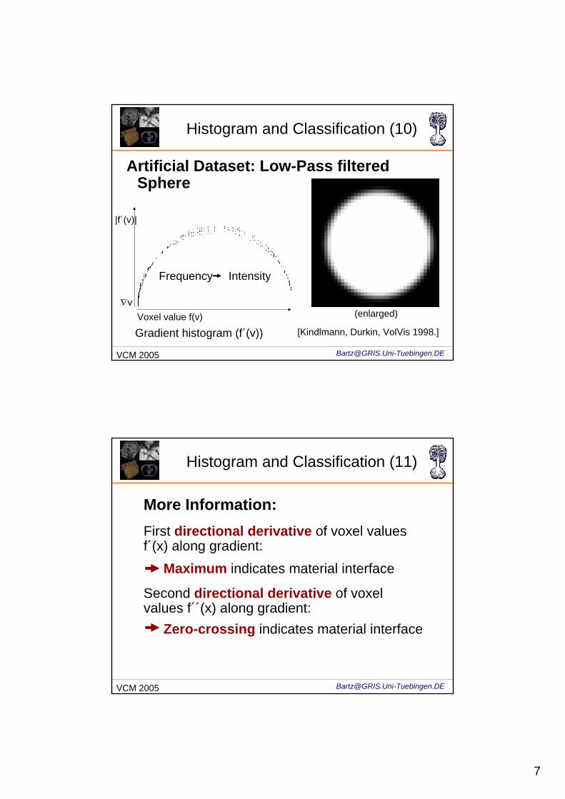
Artificial Dataset: Low-Pass filtered Sphere
(enlarged)Linear histogram
Not very informative!
7
[email protected] 2005
Histogram and Classification (10)
Artificial Dataset: Low-Pass filtered Sphere
(enlarged)
Gradient histogram (f´(v))Voxel value f(v)
∇v
|f´(v)|
Frequency Intensity
[Kindlmann, Durkin, VolVis 1998.]
[email protected] 2005
Histogram and Classification (11)
More Information:First directional derivative of voxel values f´(x) along gradient:
Maximum indicates material interface
Second directional derivative of voxel values f´´(x) along gradient:
Zero-crossing indicates material interface
8
[email protected] 2005
Histogram and Classification (12)
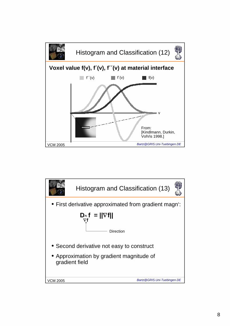
Voxel value f(v), f´(v), f´´(v) at material interface
From:[Kindlmann, Durkin, VolVis 1998.]
f(v)f´(v)f´´(v)
v
[email protected] 2005
• First derivative approximated from gradient magn‘:
D^ f = ||∇f||
• Second derivative not easy to construct
• Approximation by gradient magnitude ofgradient field
Histogram and Classification (13)
∇f
Direction
9
[email protected] 2005
Histogram and Classification (14)
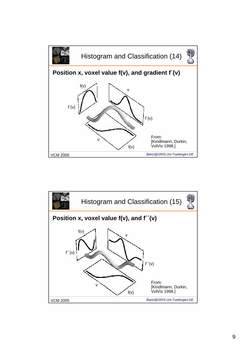
Position x, voxel value f(v), and gradient f´(v)
v
v
f(v)
f(v)
f´(v)
f´(v)
From:[Kindlmann, Durkin, VolVis 1998.]
[email protected] 2005
Histogram and Classification (15)
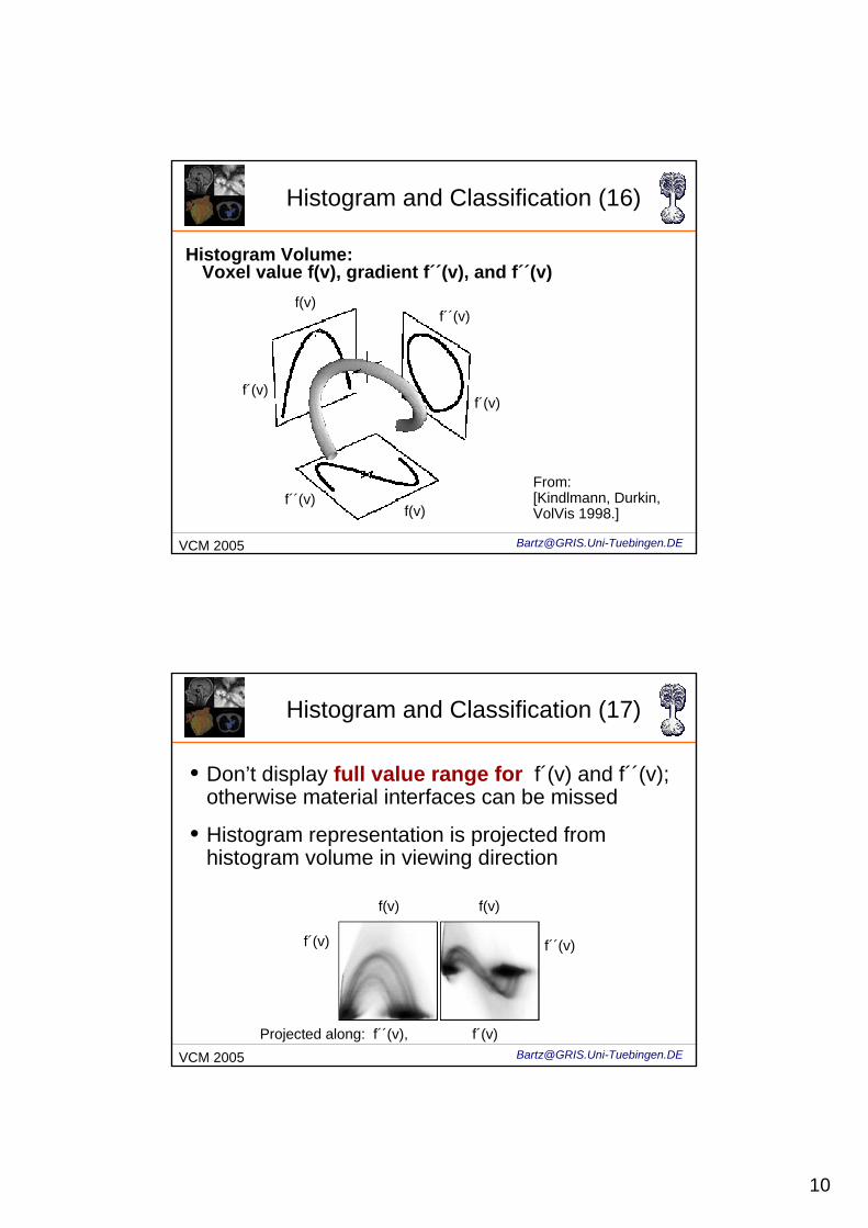
Position x, voxel value f(v), and f´´(v)
f(v)
f(v)
f´´(v)
f´´(v)
v
v From:[Kindlmann, Durkin, VolVis 1998.]
10
[email protected] 2005
Histogram and Classification (16)
Histogram Volume:Voxel value f(v), gradient f´´(v), and f´´(v)
f(v)
f(v)
f´´(v)
f´´(v)
f´(v)f´(v)
From:[Kindlmann, Durkin, VolVis 1998.]
[email protected] 2005
Histogram and Classification (17)
• Don’t display full value range for f´(v) and f´´(v); otherwise material interfaces can be missed
• Histogram representation is projected from histogram volume in viewing direction
f´(v) f´´(v)
f(v) f(v)
Projected along: f´´(v), f´(v)
11
[email protected] 2005
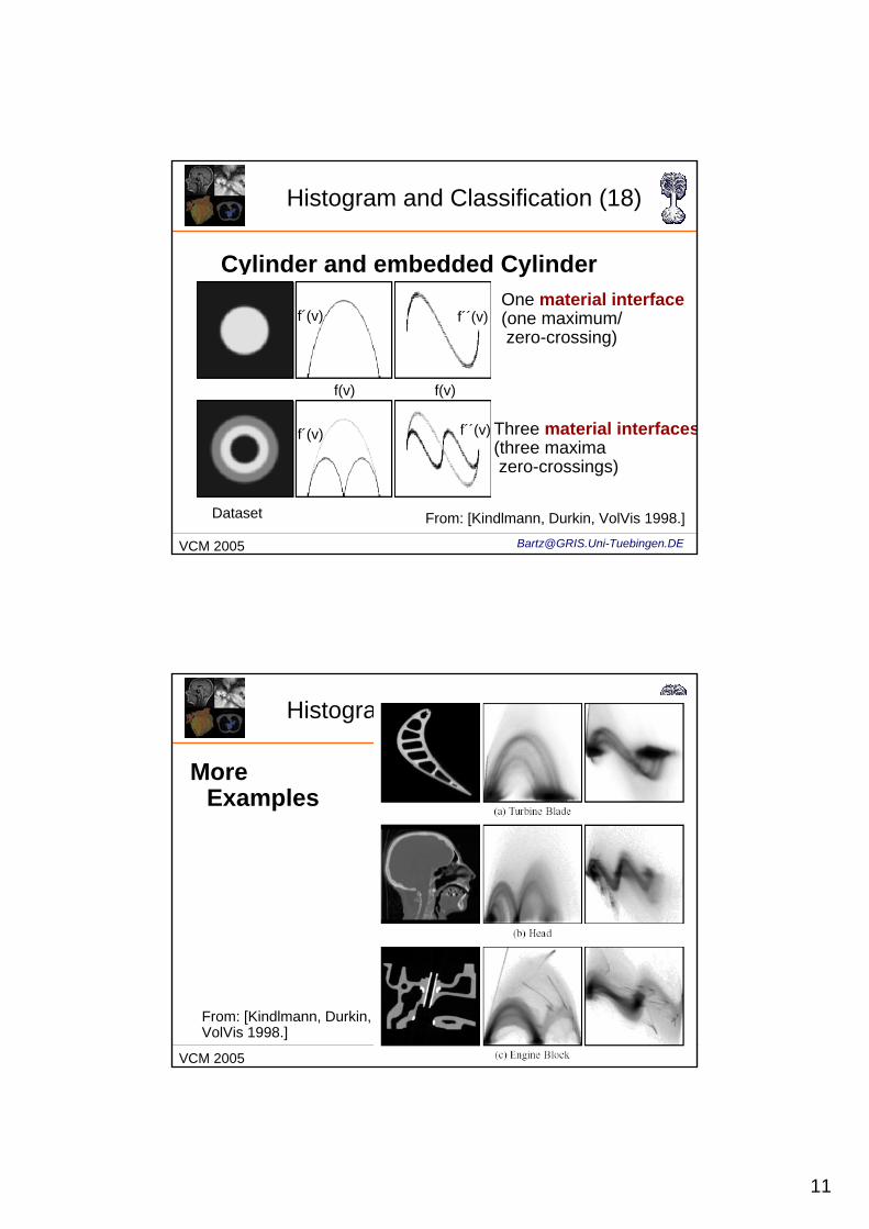
Histogram and Classification (18)
Cylinder and embedded Cylinder
Dataset
One material interface(one maximum/zero-crossing)
Three material interfaces(three maximazero-crossings)
f´(v)
f´(v) f´´(v)
f´´(v)
f(v) f(v)
From: [Kindlmann, Durkin, VolVis 1998.]
[email protected] 2005
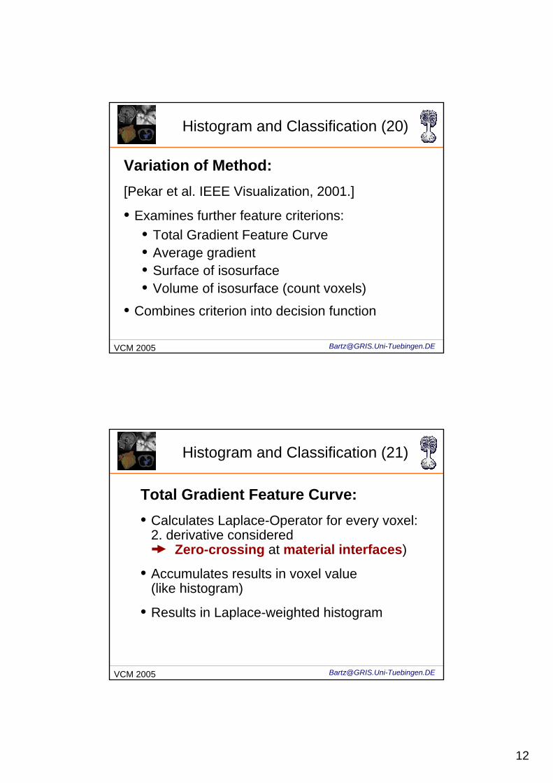
Histogram and Classification (19)
More Examples
From: [Kindlmann, Durkin, VolVis 1998.]
12
[email protected] 2005
Histogram and Classification (20)
Variation of Method:[Pekar et al. IEEE Visualization, 2001.]
• Examines further feature criterions:• Total Gradient Feature Curve• Average gradient• Surface of isosurface• Volume of isosurface (count voxels)
• Combines criterion into decision function
[email protected] 2005
Histogram and Classification (21)
Total Gradient Feature Curve:• Calculates Laplace-Operator for every voxel:
2. derivative considered Zero-crossing at material interfaces)
• Accumulates results in voxel value (like histogram)
• Results in Laplace-weighted histogram

13
[email protected] 2005
Histogram and Classification (22)
Total Gradient Feature Curve:• Features are emphasized by Maxima
Image slice Total Gradient Feature Curve 3D Rendering
From: [Pekar et al., IEEE Vis 2001.]
[email protected] 2005
Histogram and Classification (23)
Mean Gradient Feature Curve:• Divides Total Gradient Feature Curve
by measured surface along isosurface
• More independent from actual size

14
[email protected] 2005
Histogram and Classification (24)
Mean Gradient Feature Curve:• Peak size more independent of actual feature size
Image slice Mean Gradient Feature Curve 3D Rendering
From: [Pekar et al., IEEE Vis 2001 ]
[email protected] 2005
Histogram and Classification (25)
More useful metrics for Data Analysis:• Statistics of 1. order:
• Local, average gray value
mk(p(x,y)) = 1 / N ∑∑v(x+i,y+j)
• Local varianceσ2
k(p(x,y)) = 1 / (N-1) ∑∑(v(x+i,y+j) – mk(p))2
i j
k k
i j
k k
15
[email protected] 2005
Histogram and Classification (26)
More useful ...• Measure for smoothness R:
If σ2 gets small, R approaches 0 and indicates homogeneous/smooth region.
11 + σ2(p)R = 1 -
[email protected] 2005
Outline
Histograms and Classification
Windowing
Histogram Filter
Segmentation
16
[email protected] 2005
Windowing (1)
Why Windowing?• Volume Data are usually 12-16bit/voxel deep
• Output devices (screen) only have 8bit/color depth, or only 8bit gray value depth
• Value range of dataset must be mapped into 8bit
Windowing
[email protected] 2005
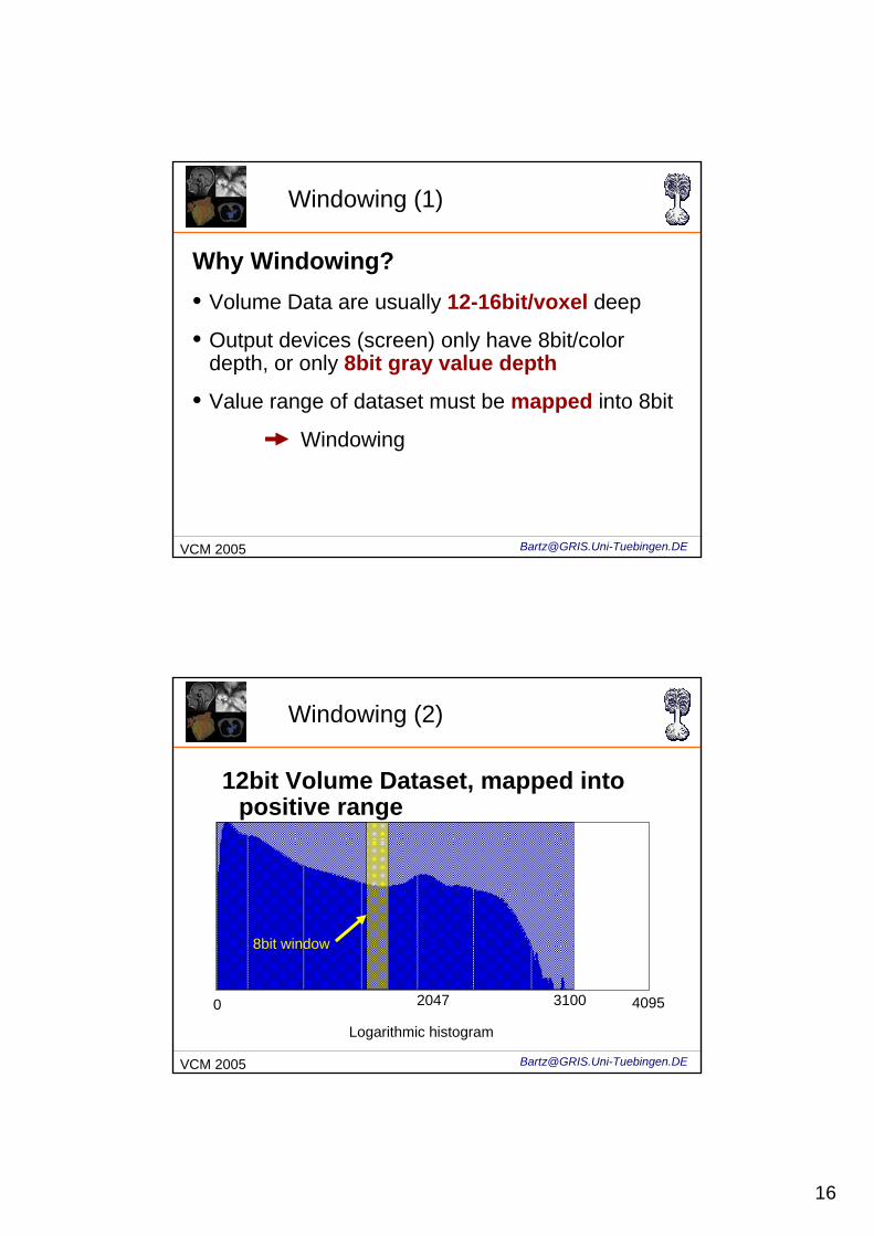
Windowing (2)
12bit Volume Dataset, mapped into positive range
0 4095
Logarithmic histogram
2047 3100
8bit window
17
[email protected] 2005
Windowing (3)
Mapping of 12bit value range into 8bit:• Selected value range is named window
• Set:• Window width• Window position (center)
• Window width controls contrast:• More wide, the smaller the contrast• More narrow, the larger the contrast
[email protected] 2005
Windowing (4)
Window Width:• Enlarging the window range with downsampling:
eg. 4bits are mapped into 1bit,or the range of 0..15 into 0..1• Loss of accuracy
• Values below/above of window are mapped on window limits: 0 or 255
18
[email protected] 2005
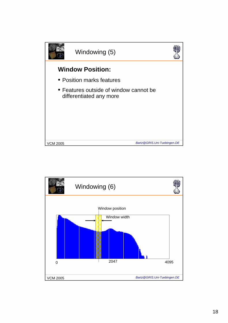
Windowing (5)
Window Position:• Position marks features
• Features outside of window cannot be differentiated any more
[email protected] 2005
Windowing (6)
0 40952047
Window width
Window position
19
[email protected] 2005
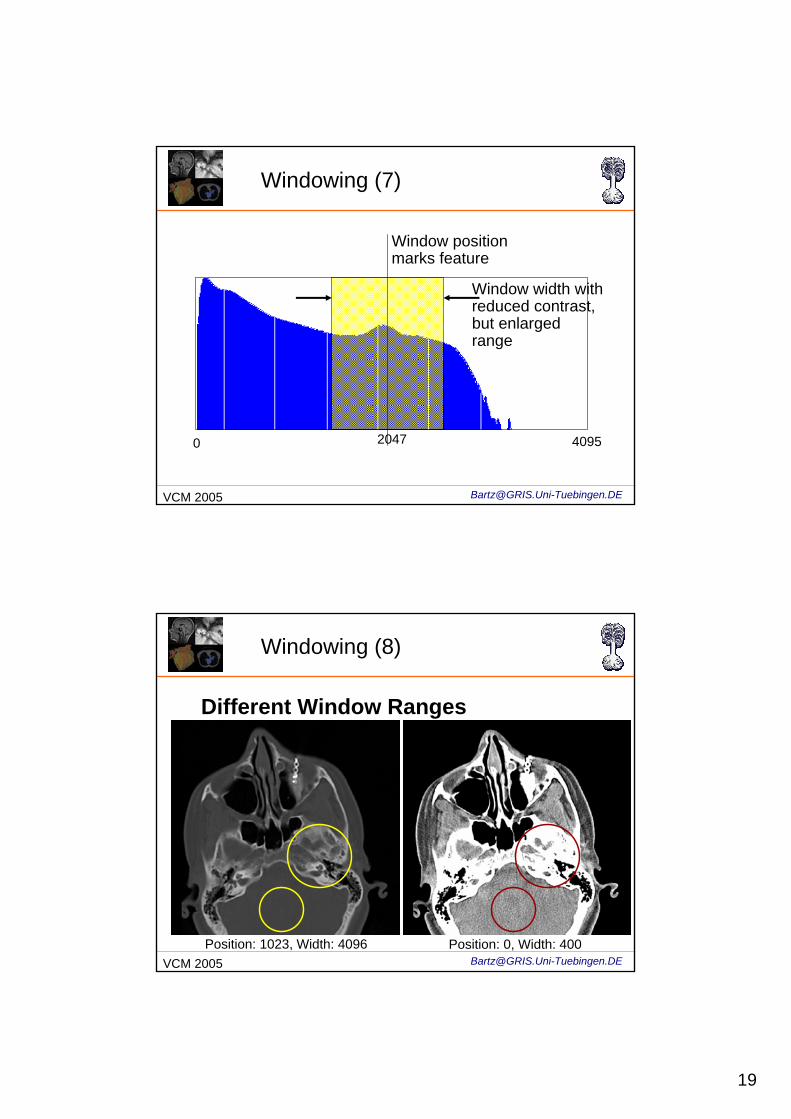
Windowing (7)
0 40952047
Window width withreduced contrast,but enlargedrange
Window position marks feature
[email protected] 2005
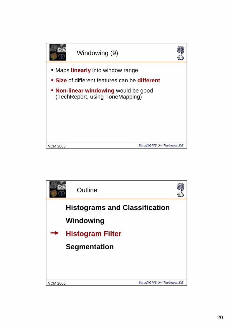
Windowing (8)
Different Window Ranges
Position: 1023, Width: 4096 Position: 0, Width: 400
20
[email protected] 2005
Windowing (9)
• Maps linearly into window range
• Size of different features can be different
• Non-linear windowing would be good(TechReport, using ToneMapping)
[email protected] 2005
Outline
Histograms and Classification
Windowing
Histogram Filter
Segmentation
21
[email protected] 2005
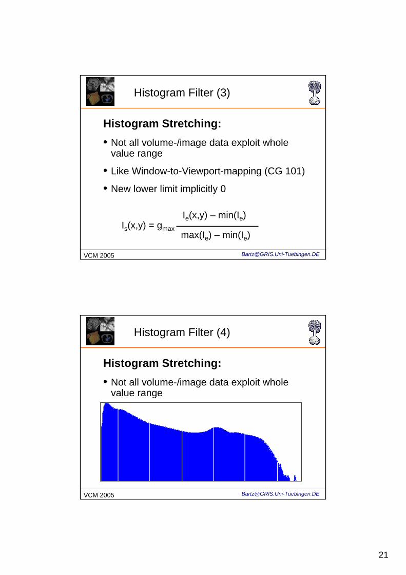
Histogram Filter (3)
Histogram Stretching:• Not all volume-/image data exploit whole
value range
• Like Window-to-Viewport-mapping (CG 101)
• New lower limit implicitly 0
Is(x,y) = gmax
Ie(x,y) – min(Ie)
max(Ie) – min(Ie)
[email protected] 2005
Histogram Filter (4)
Histogram Stretching:• Not all volume-/image data exploit whole
value range
22
[email protected] 2005
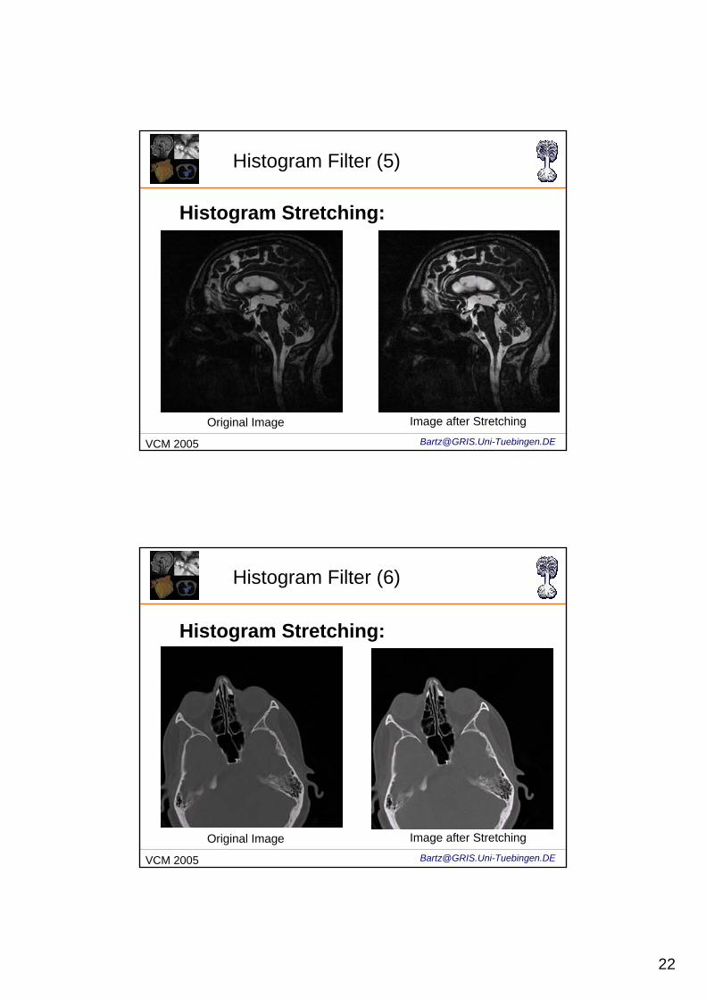
Histogram Filter (5)
Histogram Stretching:
Original Image Image after Stretching
[email protected] 2005
Histogram Filter (6)
Histogram Stretching:
Original Image Image after Stretching

23
[email protected] 2005
Histogram Filter (7)
Selective Histogram Stretching :• Partial range is mapped into larger range
• Useful to compensate for noise(not used histogram range)
• Piecewise linear
• Logarithmical
[email protected] 2005
Histogram Filter (8)
Selective Histogram Stretching:• Partial range is mapped into larger range
24
[email protected] 2005
Histogram Filter (9)
Selective Histogram Stretching:• Piecewise linear scaling:
• Regular stretching of partial range• Other ranges are kept identical (might be
translated), or culled
[email protected] 2005
Histogram Filter (10)
Selective Histogram Stretching:• Logarithmic scaling:
• Certain ranges are enhanced• More like human vision
gs(g + c3) = gmax
log(c1+ g )– log(c1)
log(c2) – log(c1)
c2 - c1
gmax
with c3 as translation in histogram, c1,c2 controlsteepness, and g as histogram.
25
[email protected] 2005
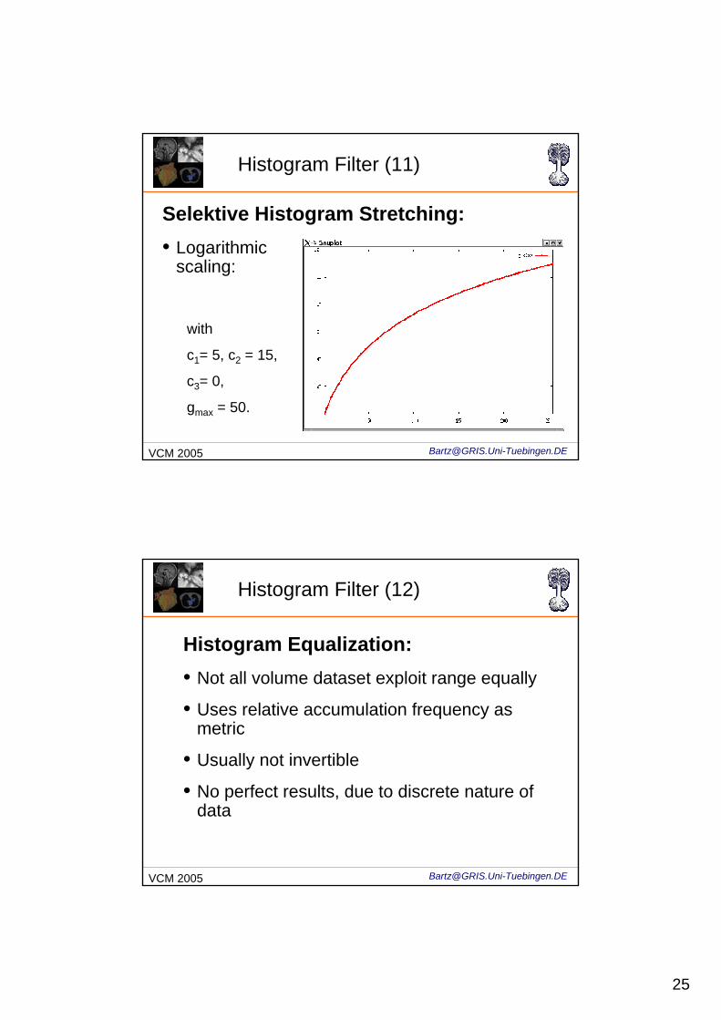
Histogram Filter (11)
Selektive Histogram Stretching:• Logarithmic
scaling:
with
c1= 5, c2 = 15,
c3= 0,
gmax = 50.
[email protected] 2005
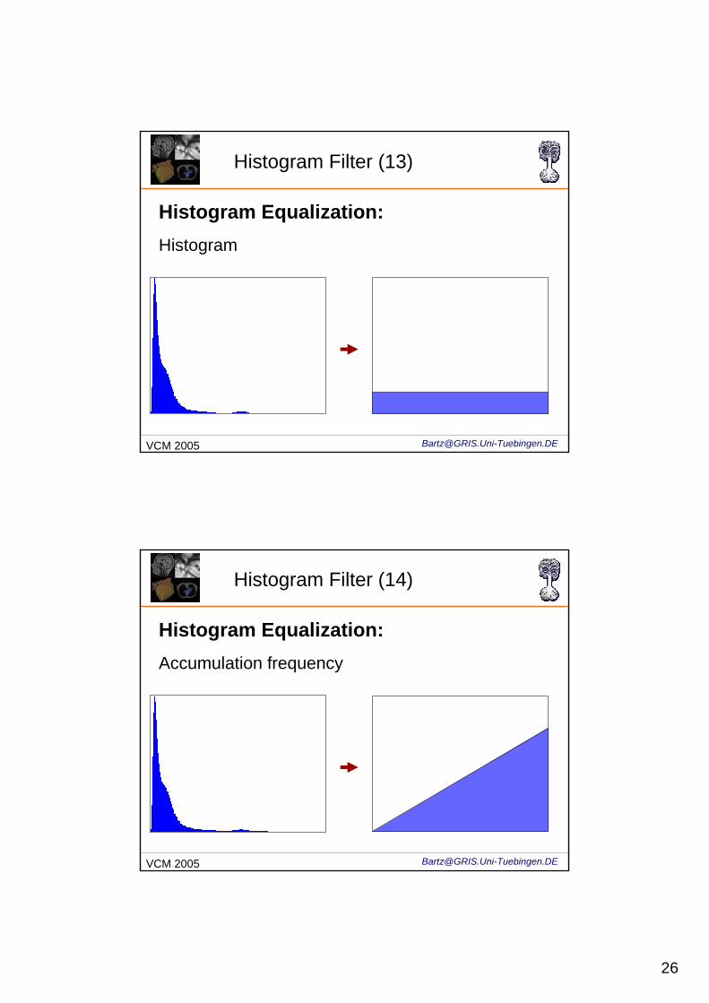
Histogram Filter (12)
Histogram Equalization:• Not all volume dataset exploit range equally
• Uses relative accumulation frequency as metric
• Usually not invertible
• No perfect results, due to discrete nature of data
26
[email protected] 2005
Histogram Filter (13)
Histogram Equalization:Histogram
[email protected] 2005
Histogram Filter (14)
Histogram Equalization:Accumulation frequency
27
[email protected] 2005
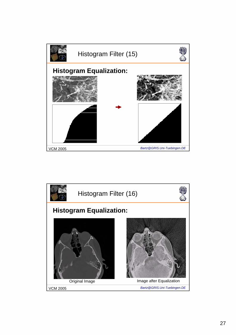
Histogram Filter (15)
Histogram Equalization:
[email protected] 2005
Histogram Filter (16)
Histogram Equalization:
Original Image Image after Equalization
28
[email protected] 2005
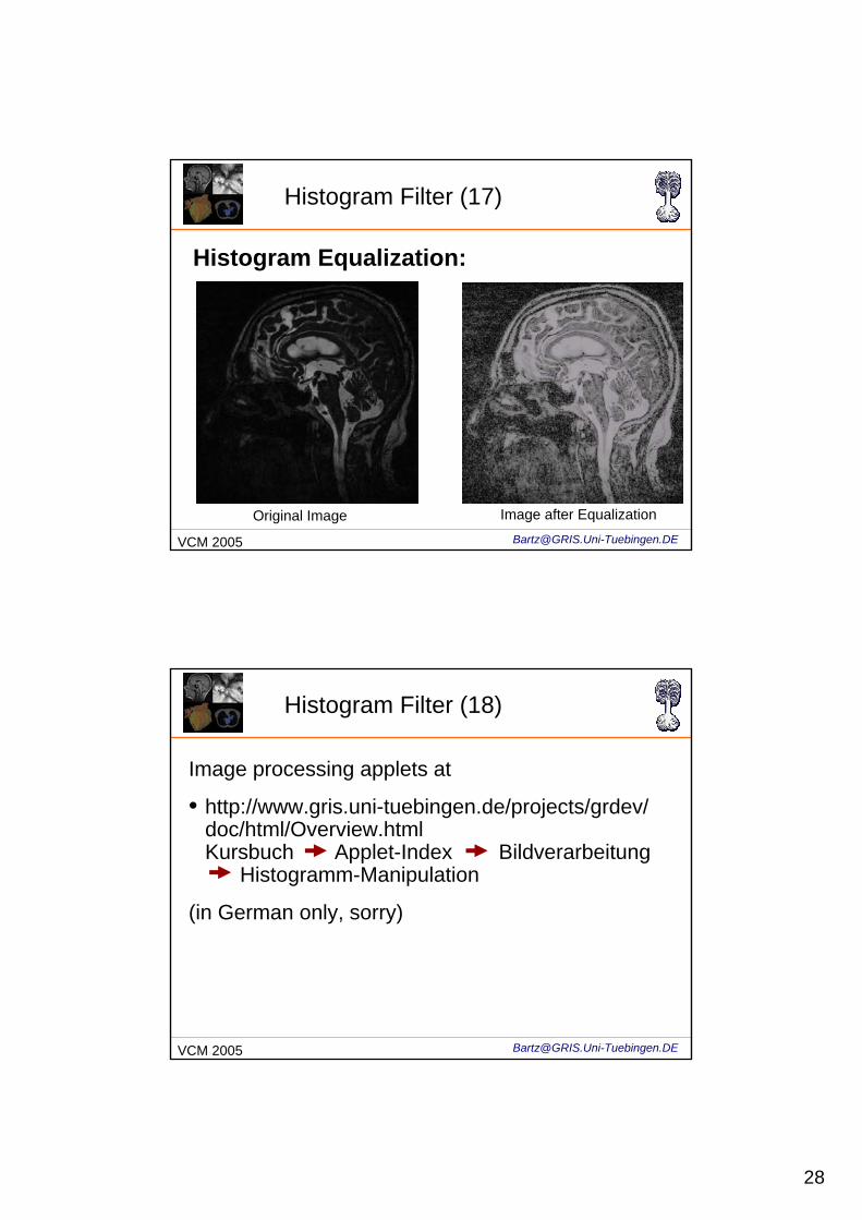
Histogram Filter (17)
Histogram Equalization:
Original Image Image after Equalization
[email protected] 2005
Histogram Filter (18)
Image processing applets at
• http://www.gris.uni-tuebingen.de/projects/grdev/doc/html/Overview.htmlKursbuch Applet-Index Bildverarbeitung
Histogramm-Manipulation
(in German only, sorry)
29
[email protected] 2005
Outline
Histograms and Classification
Windowing
Histogram Filter
Segmentation
[email protected] 2005
Segmentation (1)
What is Segmentation?• Segmentation is identification of
structures/objects (eg. organs) in image / volume data.
• Assign a semantic into data
• Unfortunately: Many structures are easy to detect with eyes, but difficult with algorithms
• Merging criterion can be local or regional.
30
[email protected] 2005
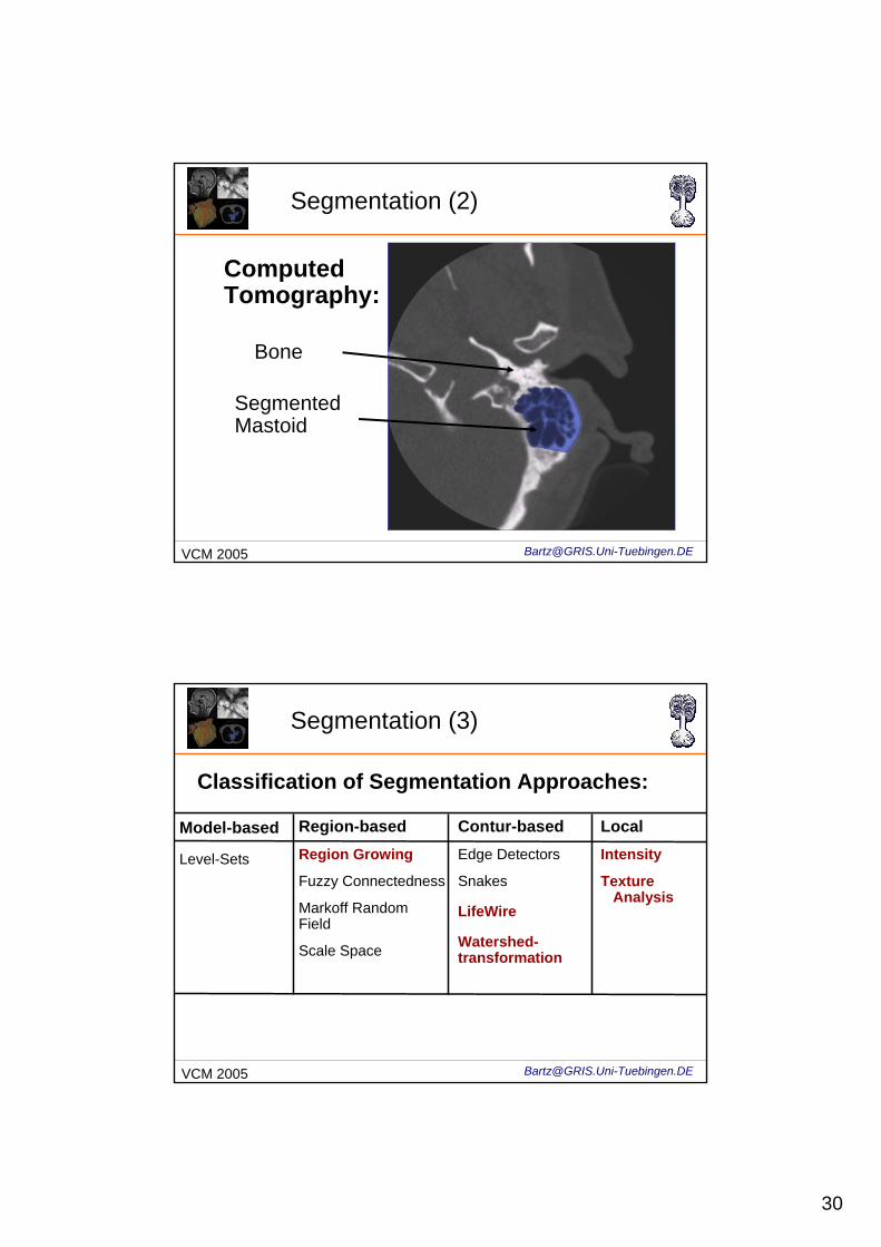
Segmentation (2)
ComputedTomography:
Bone
SegmentedMastoid
[email protected] 2005
Segmentation (3)
Classification of Segmentation Approaches:
Model-based
Level-Sets
Region-basedRegion Growing
Fuzzy Connectedness
Markoff Random Field
Scale Space
Contur-basedEdge Detectors
Snakes
LifeWire
Watershed-transformation
LocalIntensity
Texture Analysis
31
[email protected] 2005
Segmentation (5)
Segmentation:• Good data acquisition saves plenty of
segmentation work
• Sources of issues:• Partial volume effect• Insufficient resolution• Insufficient contrast• Optimal: High Intensity, Neighborhood low
intensity
[email protected] 2005
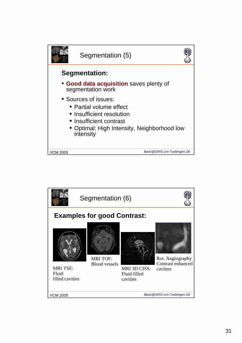
Segmentation (6)
Examples for good Contrast:
MRI TSE:Fluidfilled cavities
MRI TOF:Blood vessels
MRI 3D CISS:Fluid filled cavities
Rot. AngiographyContrast enhanced cavities

32
[email protected] 2005
Segmentation (7)
Ventricles / background
Corpus callosum / brain tissue
MRI Flash/T1
Examples of poor Contrast
[email protected] 2005
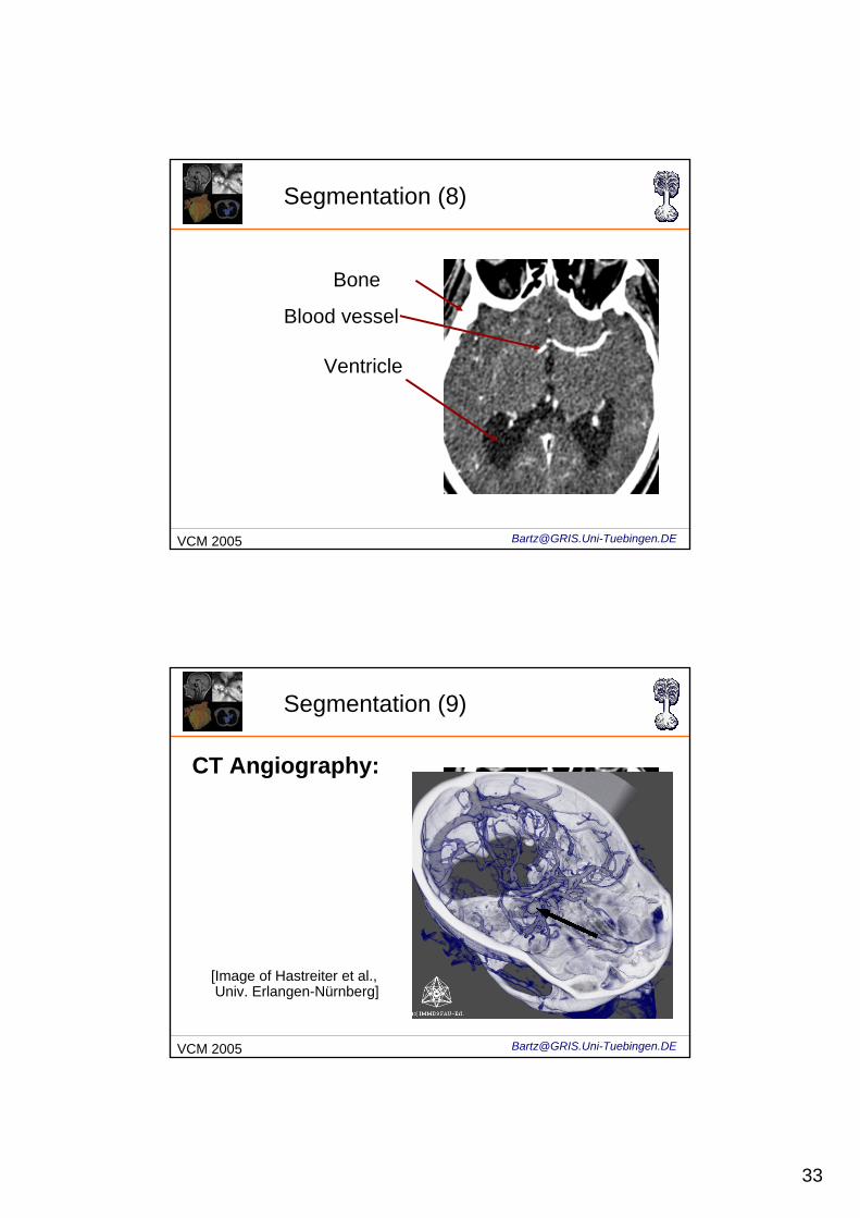
Segmentation (8)
CT Angiography:• Good bone contrast
• Good blood vessel contrast
• Poor ventricle contrast (noise)
33
[email protected] 2005
Segmentation (8)
Bone
Blood vessel
Ventricle
[email protected] 2005
Segmentation (9)
[Image of Hastreiter et al.,Univ. Erlangen-Nürnberg]
CT Angiography:

34
[email protected] 2005
Segmentation (10)
• Binary Segmentation often leads to blocky appearance due to interpolation artifacts.(similar to staircase artifacts)
Add boundary layer
[email protected] 2005
Segmentation (11)
Region-based:• Identifies Objects in 2D/3D regions
• Considers voxel neighborhood
• Needs merging criterion
35
[email protected] 2005
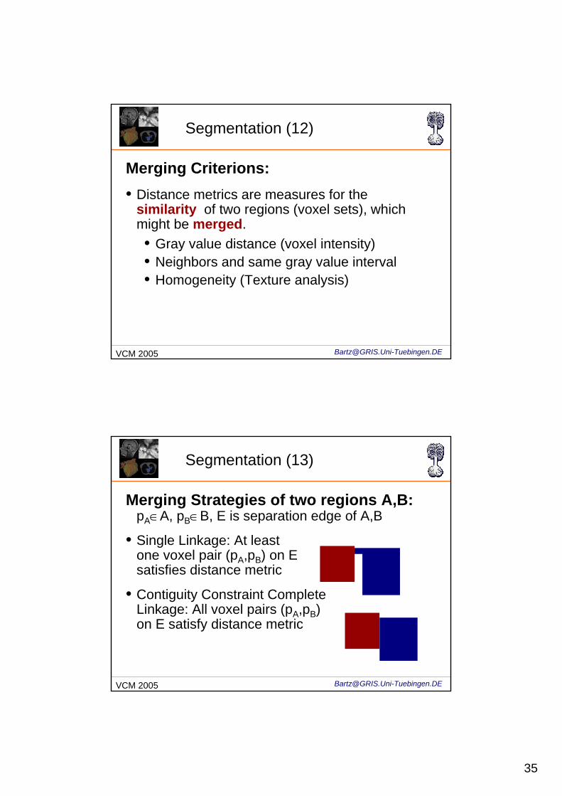
Segmentation (12)
Merging Criterions:• Distance metrics are measures for the
similarity of two regions (voxel sets), which might be merged.• Gray value distance (voxel intensity)• Neighbors and same gray value interval• Homogeneity (Texture analysis)
[email protected] 2005
Segmentation (13)
Merging Strategies of two regions A,B: pA∈A, pB∈B, E is separation edge of A,B
• Single Linkage: At least one voxel pair (pA,pB) on E satisfies distance metric
• Contiguity Constraint Complete Linkage: All voxel pairs (pA,pB) on E satisfy distance metric
36
[email protected] 2005
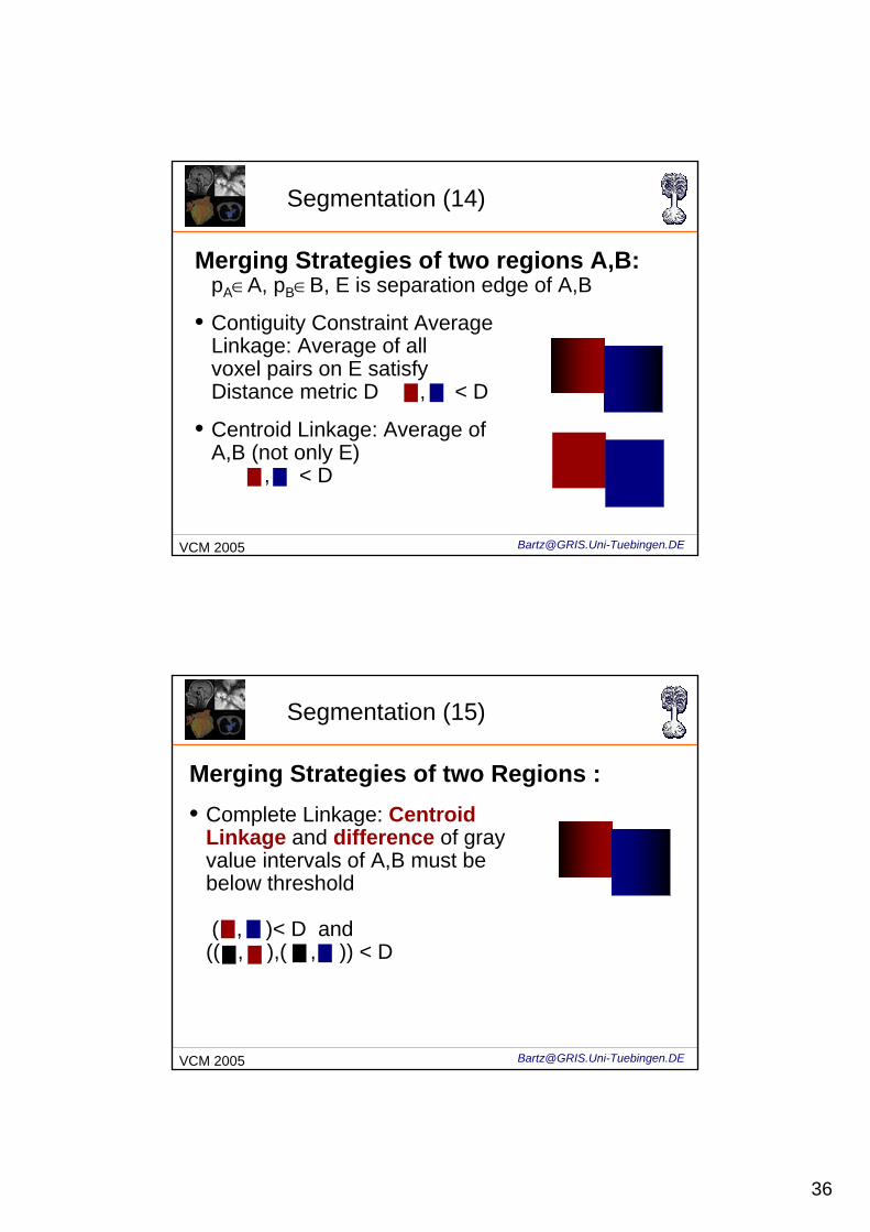
Segmentation (14)
Merging Strategies of two regions A,B: pA∈A, pB∈B, E is separation edge of A,B
• Contiguity Constraint Average Linkage: Average of all voxel pairs on E satisfy Distance metric D , < D
• Centroid Linkage: Average of A,B (not only E)
, < D
[email protected] 2005
Segmentation (15)
Merging Strategies of two Regions : • Complete Linkage: Centroid
Linkage and difference of grayvalue intervals of A,B must bebelow threshold
( , )< D and (( , ),( , )) < D
37
[email protected] 2005
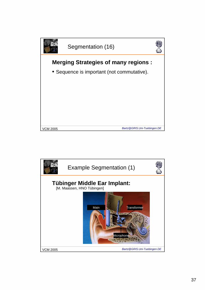
Segmentation (16)
Merging Strategies of many regions :• Sequence is important (not commutative).
[email protected] 2005
Example Segmentation (1)
Tübinger Middle Ear Implant:[M. Maassen, HNO Tübingen]
Transformer
Microphone
Main

38
[email protected] 2005
Example Segmentation (2)
Brain
Outer ear
Mastoid
[email protected] 2005
Example Segmentation (3)
• Region-oriented segmentation
• Step-wise refinement of over-segmented image data
Segmentation Correction
• Object mask• Morphology• Clipping• Connected components
• Local features• 2d/3d region growing
39
[email protected] 2005
Example Segmentation (4)
Segmentation Correction3d region growing
M1
Homogeneous image regionZK
M2
Morphological OpeningZK
2d DilatationM3
Subtraction: M1 – M3ZK
ClippingZK
M4
3d region growing.
2d region growing.M5 Subtraction: M4 – M5
[email protected] 2005
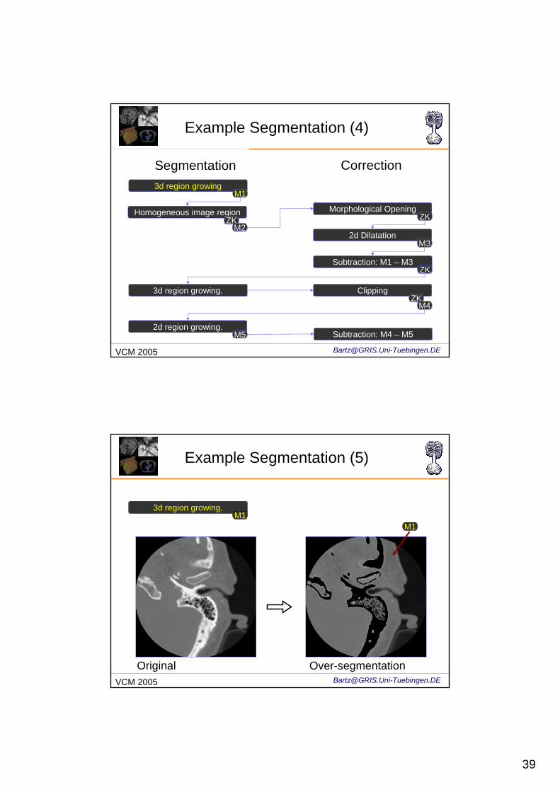
Example Segmentation (5)
Over-segmentationOriginal
M1
3d region growing.M1

40
[email protected] 2005
Example Segmentation (6)
Anatomical connectionsImage artifacts
3d region growing.M1
[email protected] 2005
Example Segmentation (7)
Segmentation Correction3d region growing.
M1
Homogeneous Image RegionZK
M2
Morphological OpeningZK
2d DilatationM3
Subtraction: M1 – M3ZK
ClippingZK
M4
3d region growing.
2d region growing.M5 Subtraction: M4 – M5

41
[email protected] 2005
Example Segmentation (8)
Homogeneous Image RegionZK
M2
Morphological OpeningZK
2d DilatationM3
Subtraction: M1 – M3ZK
[email protected] 2005
Example Segmentation (9)
Homogeneous Image RegionZK
M2
Morphological OpeningZK
2d DilatationM3
Subtraction: M1 – M3ZK
42
[email protected] 2005
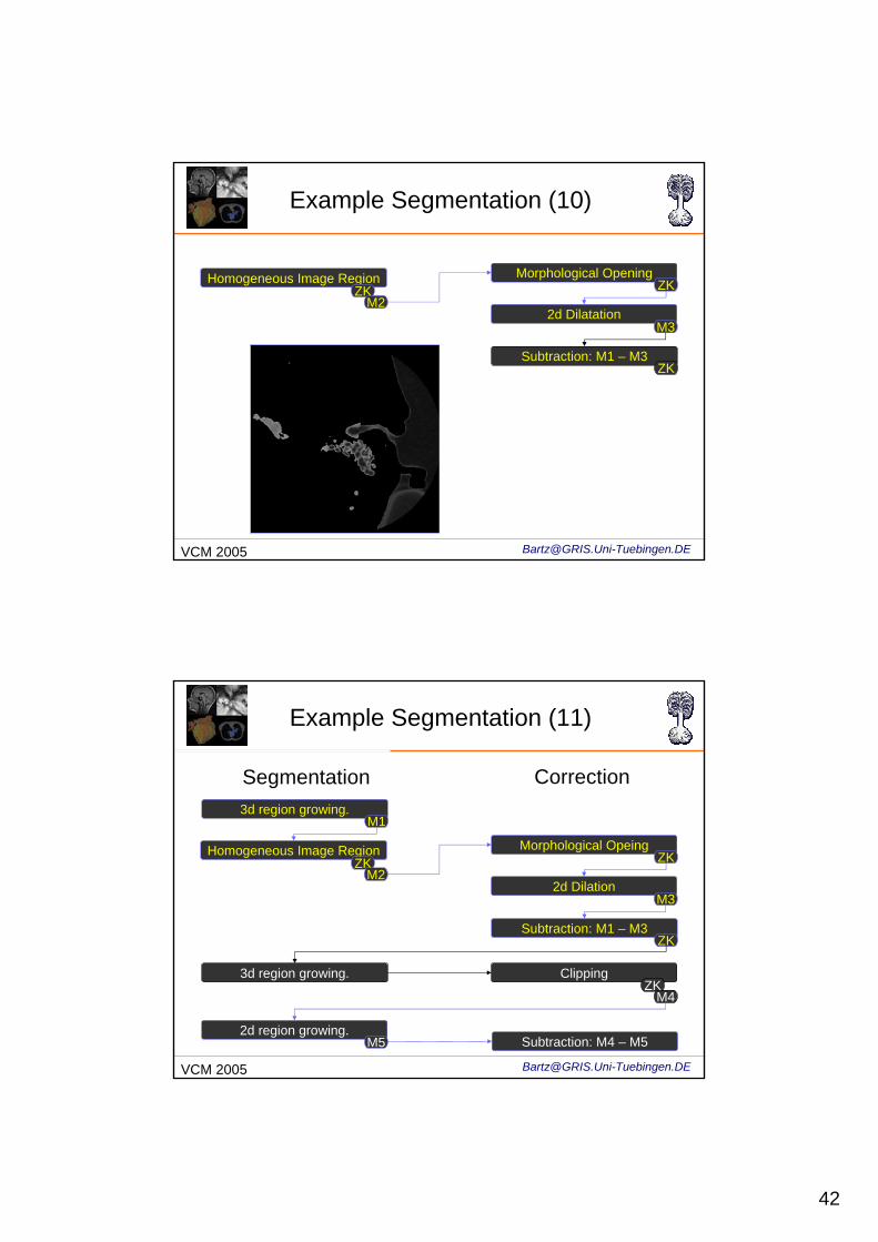
Example Segmentation (10)
Homogeneous Image RegionZK
M2
Morphological OpeningZK
2d DilatationM3
Subtraction: M1 – M3ZK
[email protected] 2005
Example Segmentation (11)
Segmentation Correction3d region growing.
M1
Homogeneous Image RegionZK
M2
Morphological OpeingZK
2d DilationM3
Subtraction: M1 – M3ZK
ClippingZK
M4
3d region growing.
2d region growing.M5 Subtraction: M4 – M5
43
[email protected] 2005
Example Segmentation (12)
3d region growing. ClippingZK
M4→ Limited grow
[email protected] 2005
Example Segmentation (13)
3d region growing. ClippingZK
M4
343536
44
[email protected] 2005
Example Segmentation (14)
Segmentation Correction3d region growing.
M1
Homogeneous Image RegionZK
M2
Morphological OpeningZK
2d DilatationM3
Subtraction: M1 – M3ZK
ClippingZK
M4
3d region growing.
2d region growing.M5 Subtraction: M4 – M5
[email protected] 2005
48
Example Segmentation (15)
2d region growing.M5 Subtraction: M4 – M5
4849 4950 50
45
[email protected] 2005
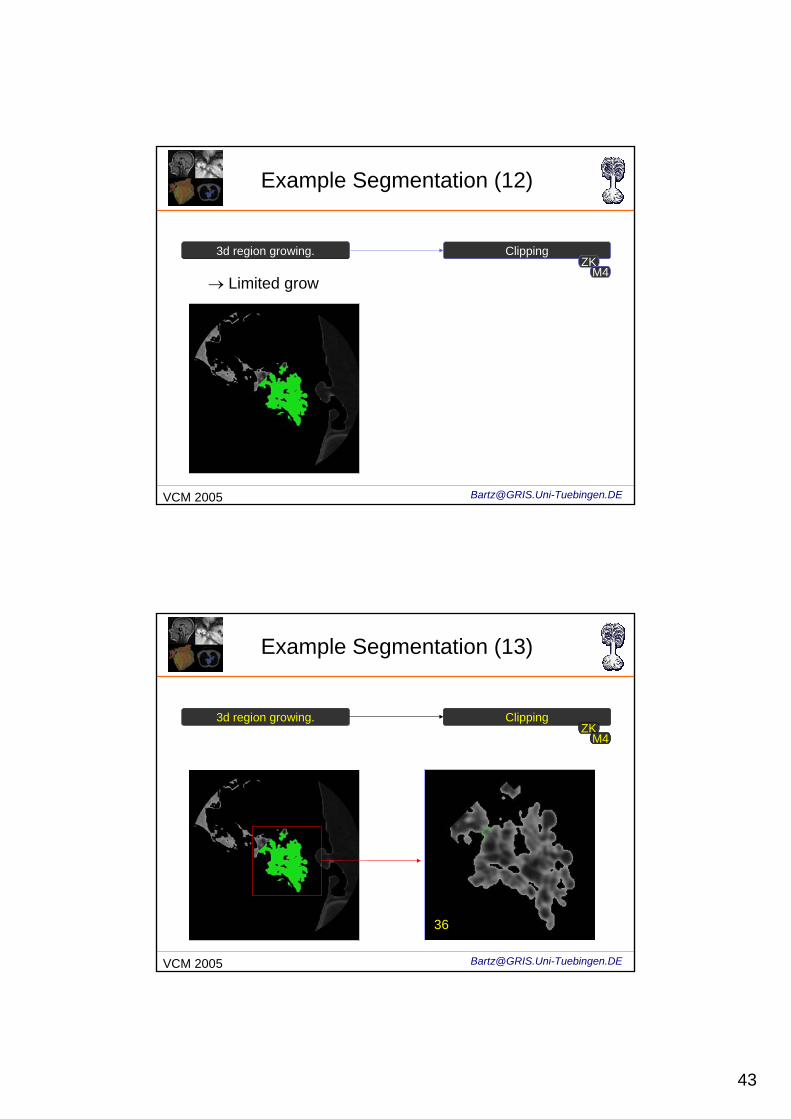
Example Segmentation (16)
Result of Segmentation:
[email protected] 2005
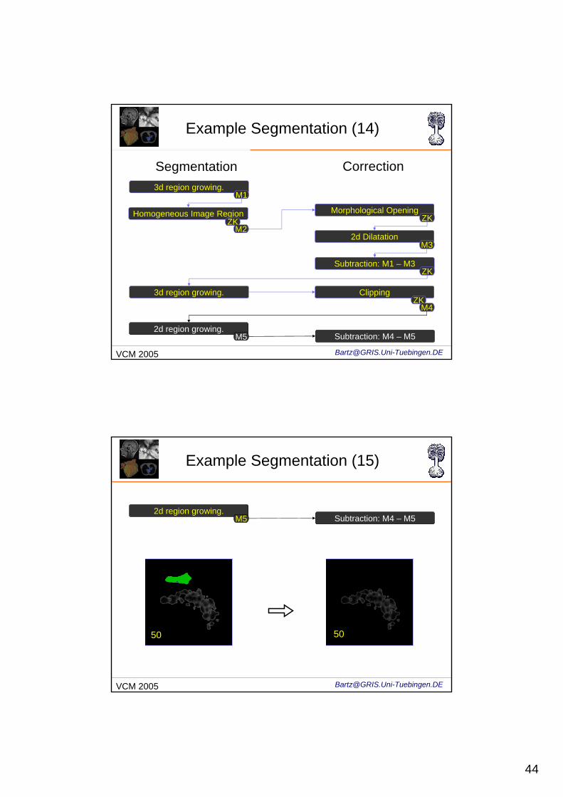
Example Segmentation (17)
Segmentation of bordering Mastoid Bone
Expansion of Mask
46
[email protected] 2005
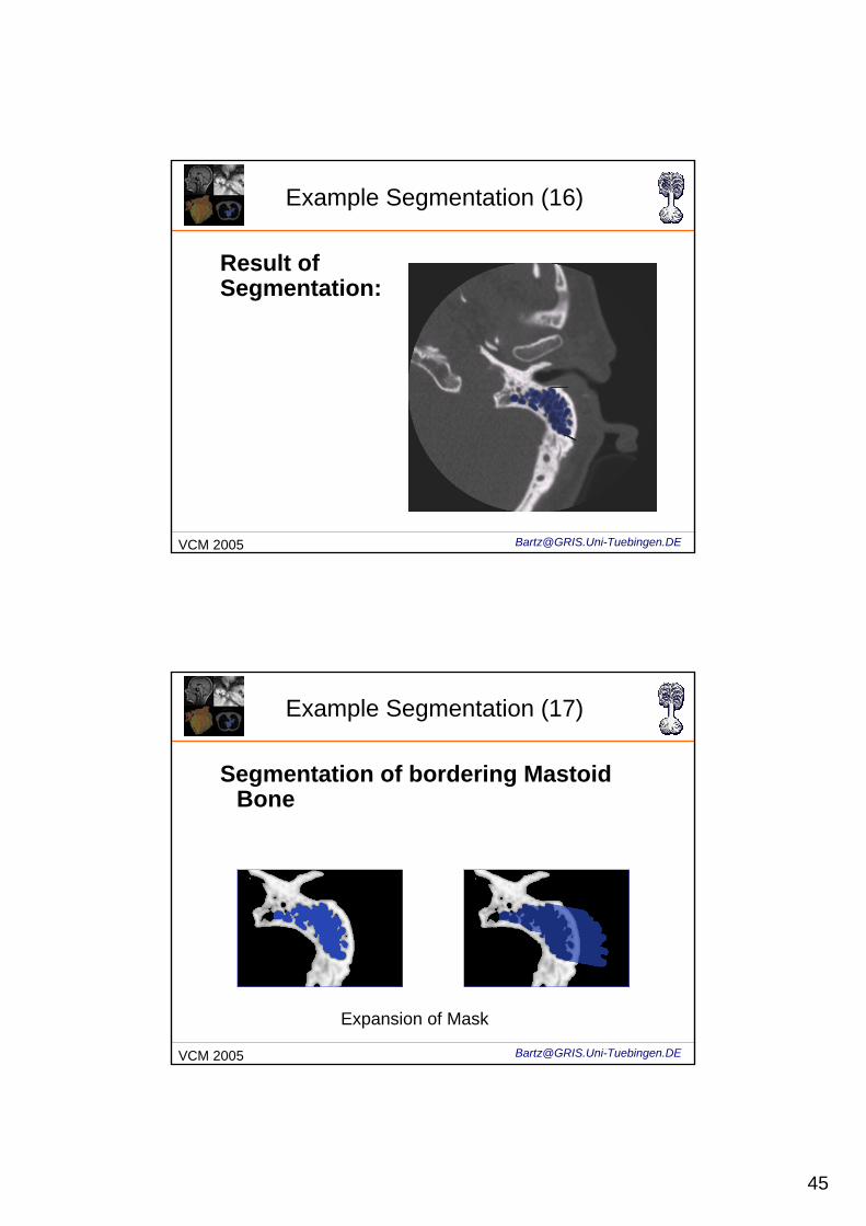
Example Segmentation (18)
Result of Segmentation:
[email protected] 2005
Image Source
• Department of Neuroradiology, University Hospital Tübingen
• Department of Radiology,University Hospital Tübingen
• Kindlmann, Durkin: VolVis 1998
• Pekar et al. IEEE Visualization 2001.