Medical Imaging Instrumentation & Image Analysis

Atam P. Dhawan, Ph.D.

Dept. of Electrical & Computer EngineeringDept. of Biomedical Engineering

New Jersey Institute of TechnologyNewark, NJ, 07102

Dhawan@adm.njit.edu

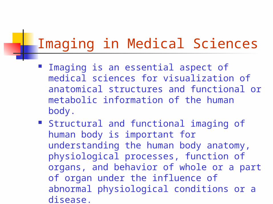
Imaging in Medical Sciences

Imaging is an essential aspect of medical sciences for visualization of anatomical structures and functional or metabolic information of the human body.

Structural and functional imaging of human body is important for understanding the human body anatomy, physiological processes, function of organs, and behavior of whole or a part of organ under the influence of abnormal physiological conditions or a disease.

Medical Imaging Radiological sciences in the last two decades have

witnessed a revolutionary progress in medical imaging and computerized medical image processing.

Advances in multi-dimensional medical imaging modalities X-ray Mammography X-ray Computed Tomography (CT) Single Photon Computed Tomography (SPECT) Positron Emission Tomography (PET) Ultrasound Magnetic Resonance Imaging (MRI) functional Magnetic Resonance Imaging (fMRI)

Important radiological tools in diagnosis and treatment evaluation and intervention of critical diseases for significant improvement in health care.

A Multidisciplinary Paradigm

Physiology and CurrentUnderstanding

Physics of Imaging

Instrumentationand Image Acquisition

Computer Processing,Analysis and Modeling

Applications andIntervention

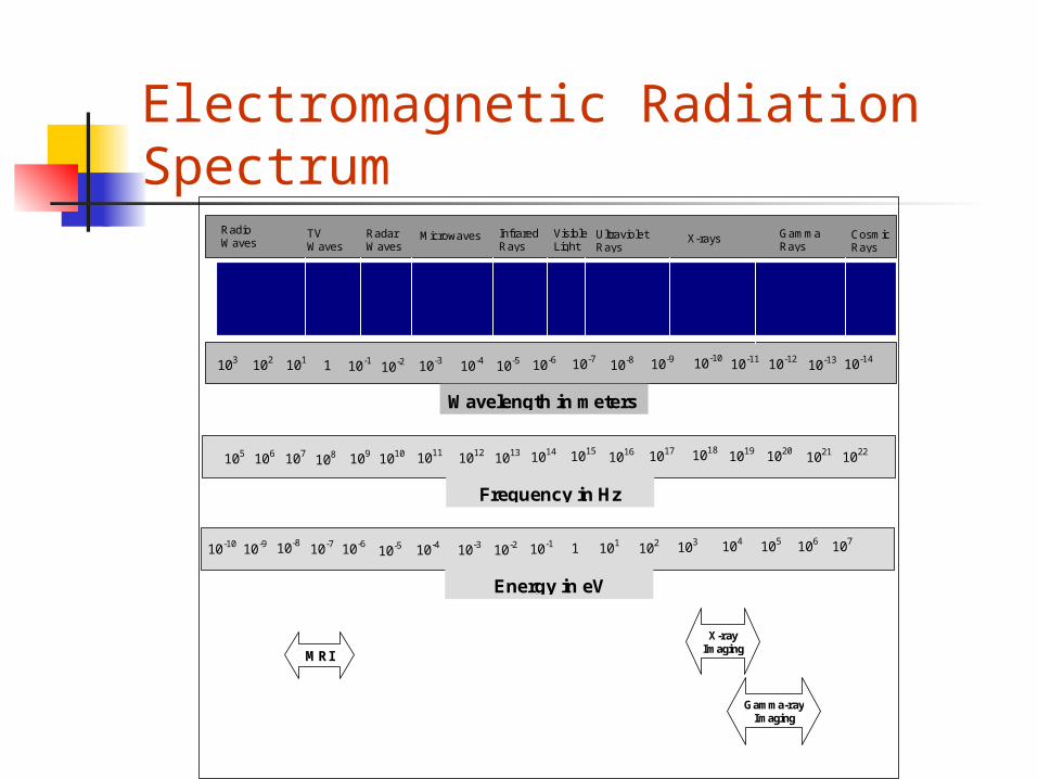
Electromagnetic Radiation Spectrum

10-10

Radio Waves

TV Waves

Radar Waves

Microwaves Infrared Rays

Visible Light

Ultraviolet Rays

X-rays Gamma Rays

102 101 1 10-1 10-2 10-3 10-4 10-6 10-7 10-8

Wavelength in meters

Frequency in Hz

10-5 10-9 10-10 10-11 10-12 10-13 10-14 103

106 107 109 1010 1011 1012 1014 1015 1016 1013 1017 1018 1019 1020 1021 1022 105 108

Energy in eV

10-9 10-8 10-6 10-5 10-4 10-3 10-1 1 101

10-2 102 103 104 105 106 107 10-7

MRI

X-ray Imaging

Gamma-ray Imaging

Cosmic Rays

Medical Imaging Information Anatomical

X-Ray Radiography X-Ray CT MRI Ultrasound Optical

Functional/Metabolic SPECT PET fMRI, pMRI Ultrasound Optical Fluorescence Electrical Impedance

Medical Imaging ModalitiesMedical Imaging Methods

Internal Combination:

Internal

& External

External

UsingEnergy Source

SPECTPET

MRIFluorescenceEI

X-RayUltrasoundOptical

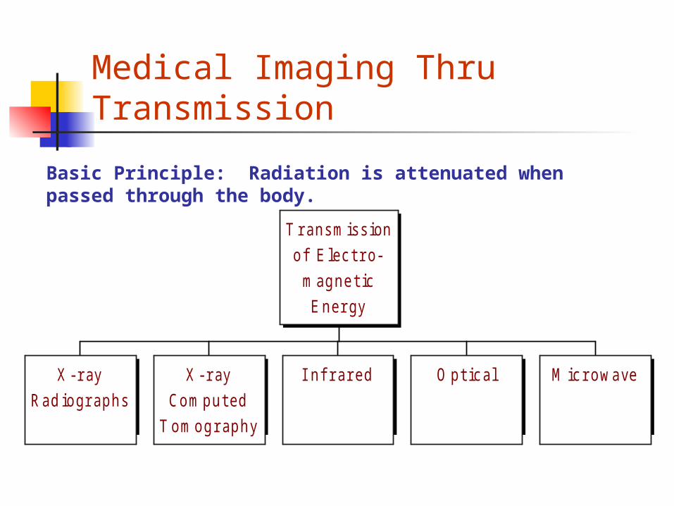
Medical Imaging Thru Transmission

X - r ay

R ad iogr aphs

X - r ay

Comput ed

T omogr aphy

I nf r ar ed O pt ic al M ic r owave

T r ansmiss ion

of E lec t r o-

magnet ic

E ner gy

Basic Principle: Radiation is attenuated when passed through the body.

ROC: Performance Measure

Ntp = Notp + Nofn and Ntn = Nofp + Notn

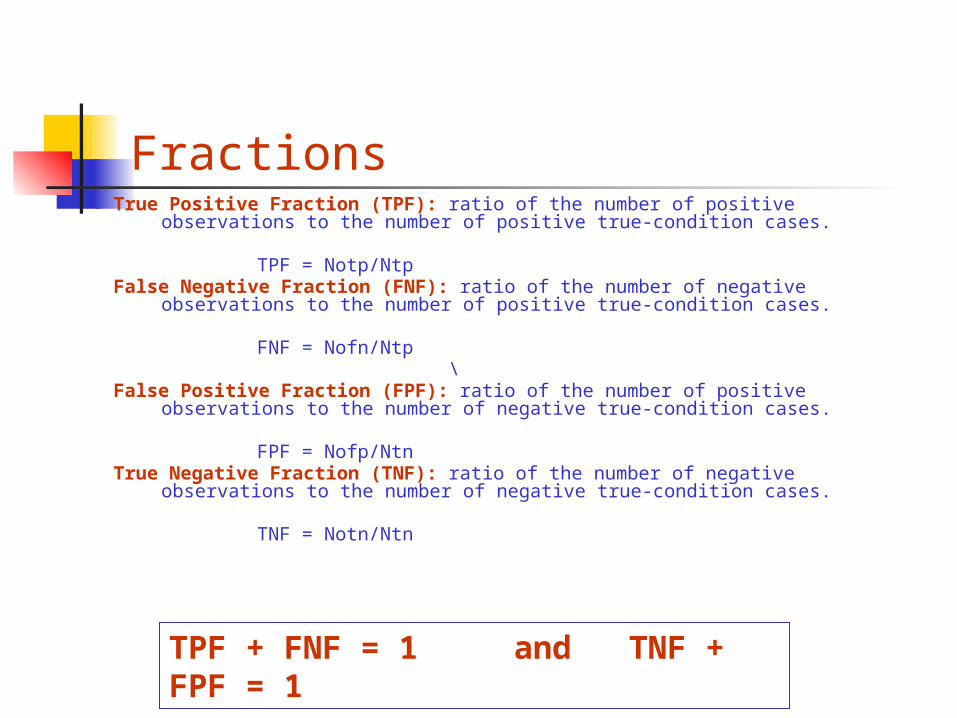
FractionsTrue Positive Fraction (TPF): ratio of the number of positive observations to the

number of positive true-condition cases.

TPF = Notp/Ntp

False Negative Fraction (FNF): ratio of the number of negative observations to the number of positive true-condition cases.

FNF = Nofn/Ntp\

False Positive Fraction (FPF): ratio of the number of positive observations to the number of negative true-condition cases.

FPF = Nofp/Ntn

True Negative Fraction (TNF): ratio of the number of negative observations to the number of negative true-condition cases.

TNF = Notn/Ntn

TPF + FNF = 1 and TNF + FPF = 1

Measures

Sensitivity is TPF

Specificity is TNF

Accuracy = (TPF+TNF)/Ntotal

ROC Curve

FPF=1-TNF

TPF

b

a

c

A Case StudyTotal number of patients = Ntot=100

Total number of patients with biopsy proven cancer (true condition of object present) = Ntp=10

Total number of patients with biopsy proven normal tissue (true condition of object NOT present) = Ntn=90

Out of the patients with cancer Ntp , the number of patients diagnosed by the physician as having cancer = Number of True Positive cases = Notp=8

Out of the patients with cancer Ntp, the number of patients diagnosed by the physician as normal = Number of False Negative cases = Nofn=2

Out of the normal patients Ntn, the number of patients rated by the physician as normal = Number of True Negative cases = Notn=85

Out of the normal patients Ntn, the number of patients rated by the physician as having cancer = Number of False Positive cases = Nofp=5

Example

True Positive Fraction (TPF) = 8/10 = 0.8

False Negative Fraction (FNF) = 2/10 = 0.2

False Positive Fraction (FPF) = 5/90 = 0.0556

True Negative Fraction (TNF) = 85/90 = 0.9444

Linear System

A system is said to be linear if it follows two properties: scaling and superposition.

)},,({)},,({)},,(),,({ 2121 zyxIbhzyxIahzyxbIzyxaIh

Image Formation: Object f, Image g

0),,(

0),,(

zyxg

f

g1(x, y,z) + g2(x, y,z) = h(x,y,z, , f1 ()) + h(x,y,z, , f2 ())

h(x,y,z, , f ()) = h(x,y,z, ) f ()

Non-negativity

Superposition

Linear Response Function

dddfzyxhzyxg )),,(,,,,,,(),,(

Image Formation

dddfzyxhzyxg ),,(),,,,,(),,(

Linear Image Formation

Image Formation

g z

Image Formation System

hObject Domain

Image Domain

a

b

x

y

Radiating Object f( , ,a b g) Image g(x,y,z)

dddfzyxhzyxg ),,(),,,,,(),,(

dddfzyxhzyxg ),,(),,(),,(

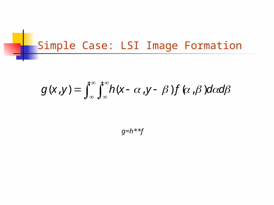
Simple Case: LSI Image Formation

ddfyxhyxg ),(),(),(

g=h**f

Image Formation: External Source

Reconstructed Cross-Sectional Image

Radiation Source

gz

Image Formation

Systemh

Object Domain

Image Domain

Selected Cross-Section

b

x

yRadiating Object

a

Image

Image Formation: Internal Source

a

gz

Reconstructed Cross-Sectional Image

Image Formation

Systemh

Object Domain

Image Domain

Selected Cross-Section

b

x

y

Radiating Object

Image

Fourier Transform

dydxeyxgyxgFTvuG vyuxj ,),()},({),( )(2

dudvevuGvuGFTyxg vyuxj

)(21 ),()},({),(

Properties of FT

b

v

a

uG

abbyaxg ,

1)},(FT

Scaling: It provides a proportional scaling.

FT {ag(x,y)+bh(x,y)}= aFT{g(x,y)+ bFT{h(x,y)

Linearity: Fourier transform, FT, is a linear transform.

FT Properties

)(2),()},({ vbuajevuGbyaxgFT

),(),(),(),( vuHvuGddyxhgFT

),(*),(),(*),( vuHvuGddyxhgFT

Translation

Convolution

Cross-Correlation

FT Properties….

2),(),(*),(),(*),( vuGvuGvuGddyxggFT

dudvvuGvuGdxdyyxgyxg ),(*),(),(*),(

)}({)}({)},({

)()(),(

ygFTxgFTyxgFT

then

ygxgyxg

yyxx

yx

Auto-Correlation

Parseval’s Theorem

Separability

Radon Transform

x

y

q

q

p

q

p

f(x,y)

P(p,q)

Line integral projection P(p,q) of the two-dimensional Radon transform.

Radon TransformProjection p1

Projection p2

Projection p3

Reconstruction Space

A

B

dqqpqpfpJyxfR )cossin,sincos()()},({

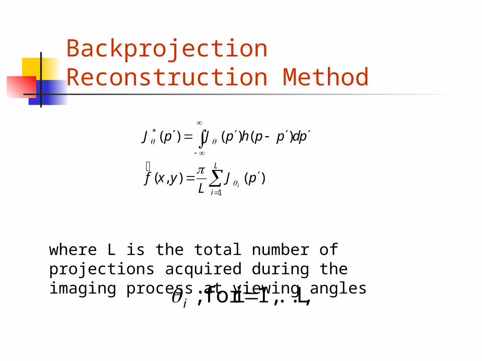
Backprojection Reconstruction Method

L

i

pJL

yxf

pdpphpJpJ

i1

*

)(),(

)()()(

where L is the total number of projections acquired during the imaging process at viewing angles

L .., 1, ifor ; i

Sampling Theorem

The sampling theorem provides the mathematical foundation of Nyquist criterion to determine the optimal sampling rate for discretization of an analog signal without the loss of any frequency information.

The Nyquist criterion states that to avoid any loss of information or aliasing artifact, an analog signal must be sampled with a sampling frequency that is at least twice the maximum frequency present in the original signal.

Sampling

1 2

),(),( 21j j

yjyxjxyxs

1 2

),(),(),(),(f y][x,f 2121adj j

a yjyxjxyjxjfyxsyx

The sampled version of the image, fd[x,y] is obtained from sampling the analog version as

Sampling Effect In Fourier domain the spectrum overlapping has to be

avoided by proper sampling of the image in spatial domain. Sampling in spatial domain produces a convolution in the

frequency domain.

xs = 2/x and xy = 2/y

1 2

),(1

),( 21j j

ysyxsxayxs jjFyx

F

where Fa(x,y) is the Fourier transform of the analog image fa(x,y) and xs and xy represent the Fourier domain sampling spatial frequencies such that

To avoid overlapping of image spectra, it is necessary that

xs >= xmax = 2fxmax and ys >= ymax = 2fymax

Nyquist (Optimal) Sampling

wx

wy

wymax

wxmax-wxmax

-wymax

Fa(wx,wy)

(a)

(b)

(c)

xs >= xmax = 2fxmax and ys >= ymax = 2fymax

Wavelet Transform

Fourier Transform only provides frequency information.

Windowed Fourier Transform can provide time-frequency localization limited by the window size.

Wavelet Transform is a method for complete time-frequency localization for signal analysis and characterization.

Wavelet Transform..

Wavelet Transform : works like a microscope focusing on finer time resolution as the scale becomes small to see how the impulse gets better localized at higher frequency permitting a local characterization

Provides Orthonormal bases while STFT does not.

Provides a multi-resolution signal analysis approach.

Wavelet Transform…

Using scales and shifts of a prototype wavelet, a linear expansion of a signal is obtained.

Lower frequencies, where the bandwidth is narrow (corresponding to a longer basis function) are sampled with a large time step.

Higher frequencies corresponding to a short basis function are sampled with a smaller time step.

Continuous Wavelet Transform

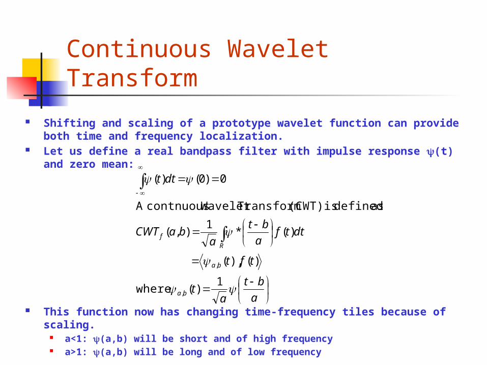
Shifting and scaling of a prototype wavelet function can provide both time and frequency localization.

Let us define a real bandpass filter with impulse response y(t) and zero mean:

This function now has changing time-frequency tiles because of scaling. a<1: y(a,b) will be short and of high frequency a>1: y(a,b) will be long and of low frequency

a

bt

at

tft

dttfa

bt

abaCWT

dtt

ba

ba

R

f

1)( where

)(),(

)(*1

),(

as defined is (CWT) Transform Wavelet contnuousA

0)0()(

,

,

Wavelet Decomposition

T h e w a v e l e t t r a n s f o r m o f a s i g n a l i s i t s d e c o m p o s i t i o n o n a f a m i l y o fr e a l o r t h o n o r m a l b a s e s

m n ( x ) o b t a i n e d t h r o u g h t r a n s l a t i o n a n dd i l a t i o n o f a k e r n e l f u n c t i o n ( x ) k n o w n a s t h e m o t h e r w a v e l e t .

W h e r e m , n Z , a s e t o f i n t e g e r s

)2(2)( 2/, nxx mm

nm

Wavelet Coefficients

Using orthonormal property of the basis functions, wavelet coefficients of a signal f(x) can be computed as

The signal can be reconstructed from the coefficients as

)()()( ,, xdxxfd nmnm

)()( ,, xdxf nmm n

nm

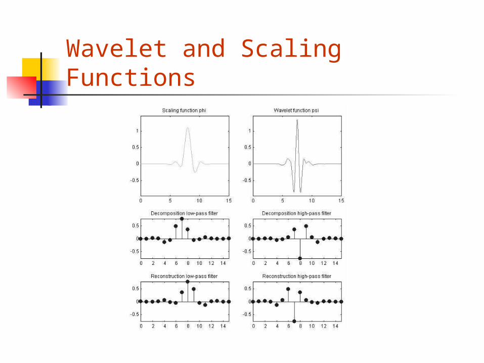
Wavelet Transform with Filters The mother wavelet can be constructed using a scaling

function f(x) which satisfies the two-scale equation

Coefficients h(k) have to meet several conditions for the set of basis functions to be unique, orthonormal and have a certain degree of regularity.

For filtering operations, h(k) and g(k) coefficients can be used as the impulse responses correspond to the low and high pass operations.

)()1()(

)2()(2)(

)2()(2)(

klk

where

nxnx

nxnx

k

n

n

hg

g

h

Decomposition

H H

G

H

G

G

2 2

2

2

2

Data

Wavelet Decomposition Space

V0 data

V1 W1

V2 W2

V3 W3

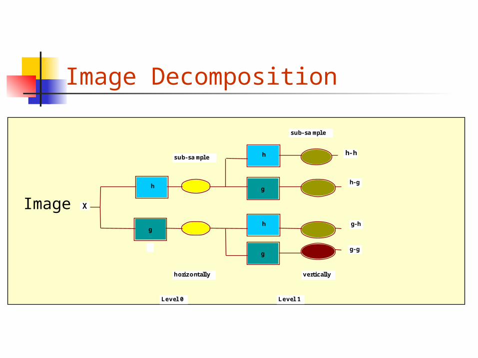
Image Decomposition

h g

sub-sample

Level 0 Level 1

h- h

h-g

g-h

g-g

horizontally vertically

sub-sample

g

gh

h

XImage

Wavelet and Scaling Functions

Image Processing and Enhancement