DI

SC

US

SI

ON

P

AP

ER

S

ER

IE

S

Forschungsinstitut zur Zukunft der ArbeitInstitute for the Study of Labor

Medical Technology and the Production of Health Care

IZA DP No. 5545

March 2011

Badi H. BaltagiFrancesco MosconeElisa Tosetti

Medical Technology and the Production of Health Care

Badi H. Baltagi Syracuse University,

University of Leicester and IZA

Francesco Moscone Brunel University

Elisa Tosetti

University of Cambridge

Discussion Paper No. 5545 March 2011

IZA

P.O. Box 7240 53072 Bonn

Germany

Phone: +49-228-3894-0 Fax: +49-228-3894-180

E-mail: iza@iza.org

Any opinions expressed here are those of the author(s) and not those of IZA. Research published in this series may include views on policy, but the institute itself takes no institutional policy positions. The Institute for the Study of Labor (IZA) in Bonn is a local and virtual international research center and a place of communication between science, politics and business. IZA is an independent nonprofit organization supported by Deutsche Post Foundation. The center is associated with the University of Bonn and offers a stimulating research environment through its international network, workshops and conferences, data service, project support, research visits and doctoral program. IZA engages in (i) original and internationally competitive research in all fields of labor economics, (ii) development of policy concepts, and (iii) dissemination of research results and concepts to the interested public. IZA Discussion Papers often represent preliminary work and are circulated to encourage discussion. Citation of such a paper should account for its provisional character. A revised version may be available directly from the author.

IZA Discussion Paper No. 5545 March 2011

ABSTRACT

Medical Technology and the Production of Health Care* This paper investigates the factors that determine differences across OECD countries in health outcomes, using data on life expectancy at age 65, over the period 1960 to 2007. We estimate a production function where life expectancy depends on health and social spending, lifestyle variables, and medical innovation. Our first set of regressions include a set of observed medical technologies by country. Our second set of regressions proxy technology using a spatial process. The paper also tests whether in the long-run countries tend to achieve similar levels of health outcomes. Our results show that health spending has a significant and mild effect on health outcomes, even after controlling for medical innovation. However, its short-run adjustments do not seem to have an impact on health care productivity. Spatial spill overs in life expectancy are significant and point to the existence of interdependence across countries in technology adoption. Furthermore, nations with initial low levels of life expectancy tend to catch up with those with longer-lived populations. JEL Classification: C31, C33, H51 Keywords: life expectancy, health care production, health expenditure, spatial dependence Corresponding author: Francesco Moscone Brunel Business School Brunel University Uxbridge Middlesex UB8 3PH United Kingdom E-mail: francesco.moscone@brunel.ac.uk

* Francesco Moscone and Elisa Tosetti acknowledge financial support from ESRC (Ref. no. RES-061-25-0317). We thank two anonymous referees, Alberto Holly, Stephen Hall, John Mullahy, Edward Norton, Andrew Jones, and the participants of the II Health Econometrics Workshop, held in Rome in July 2010.

1 Introduction

The last few decades have witnessed rapid growth in health expenditure. From 1960 to 2007,health care expenditure in OECD countries increased, on average, from 3.8 per cent to 9.0 percent of GDP. Considerable attention has been given to understanding the factors that haveproduced such growth. This includes looking at the relationship between health spending andincome, and reviving economic theories linked to the low productivity of the health sector, suchas the Baumol (1967) cost disease theory. An alternative explanation for the rise in healthspending is that over time people tend to demand and obtain higher quality of health care(Skinner et al., 2005). There continues to be a live discussion on whether, ceteris paribus, higherhealth spending corresponds to better health outcomes. A number of empirical studies supportthe hypothesis of a �at curve of health care expenditure, namely that more spending does nothave a signi�cant impact on health outcomes (Fisher et al., 2003; Skinner et al., 2005; Fisheret al., 2009). Other studies, for example the work by Baicker and Chandra (2004), even �nd anegative correlation between health quality measures and health spending.

Jones (2002) formalizes and empirically tests a model where health expenditure and lifeexpectancy are endogenous variables driven by technological progress. He �nds little associationbetween changes in life expectancy and changes in health expenditure (as a share of GDP) inthe US. However, interestingly enough, the author also �nds that a large fraction of the increasein health spending over time is driven by medical advances. Hall and Jones (2007) estimate anhealth production function for the US that relates age-speci�c mortality rates to health spendingand technology. Their �nding support the theory that the rising health expenditure relative toincome occurs as consumption of non-health goods and services grows more slowly than income.As people get richer and saturated with non-health consumption, they become more willing todevote their resources to purchase additional years of life. Skinner and Staiger (2009) develop amacroeconomic model of productivity and technology di¤usion to explain persistent productivitydi¤erences across US hospitals. Focusing on US Medicare data, they �nd that cost-e¤ectivemedical innovations explain a large fraction of persistent variability in hospital productivity,and swamp the impact of traditional factor inputs. Additionally, they argue that there is aclear polarization in health care productivity between hospitals that usually tend to adopt lesstechnology, the so-called �tortoises�, and those that traditionally adopt more technology, the�tigers�. Survival rates in low-di¤usion hospitals lag by roughly a decade behind high-di¤usionhospitals.

That technological progress has an important impact both on health outcomes and spend-ing is well known. Medical advances allow ill people that could not be treated in the past tobe cured today. In some cases, technology progressively reduces the cost of treatments. Forexample, in the case of acute myocardial infarction, new technologies have the characteristic ofbeing less invasive, ultimately reducing hospital stays, rehabilitation times, and health costs.The less invasive coronary stents delivered percutaneously, as well as drug eluting stents, aregradually taking over bypass surgery. Using US data, Cutler and Huckman (2003) examinethe di¤usion over the past two decades of percutaneous coronary interventions to treat coronary

2

artery disease. They �nd that percutaneous coronary interventions improve health productivity,especially when substituting more invasive and expensive interventions such as coronary arterybypass graft surgery. In recent years, pharmaceuticals such as statins were dispensed for pre-vention, proving to be e¤ective in reabsorbing atherosclerotic plaques and hence reducing theneed for angioplasty, and the associated costs. We refer to Moise (2003) for further discussionon how technological change a¤ects health expenditures.

This paper models di¤erences across OECD countries in health productivity as a function oftraditional factor inputs, life styles conditions, technological progress. In our empirical exercisewe �rst explore available data on medical technology to explain health productivity in the OECDcountries. However, given the paucity of the data and the di¢ culty in measuring medicaltechnology at the country level, we assume that technology is unobserved, and proxy for itby means of a spatial process. Our set-up is similar to that proposed by Ertur and Koch(2007) and Frischer (2010), where we allow technological progress in a country to be related tothe technology adopted by neighboring countries. That technology may show a geographicalpattern is well known in the economic literature (see, for example, Keller (2004)). In themedical literature, a consolidated body of research supports the important role of interpersonalcommunication and social networks in the di¤usion of medical technologies (see, for example,the classic di¤usion study by Coleman, Katz and Menzel, (1966)). We refer to Birke (2009)for a survey on the role of social networks in explaining individual choices in a large varietyof economic, social and health behavior. Communication and information sharing may occurnot only within national boundaries, but also across countries through social interaction inconferences, training or visiting programs, or the publication of results from clinical studiesinvolving medical technologies. For example, Tu et al. (1998) demonstrated a strong correlationbetween the publication of studies on the use of a particular technology in the prevention of strokeand the corresponding rates of utilization in the US and Canada. They show that utilizationrates increased dramatically between 1989 and 1995 following the publication of two in�uentialclinical studies demonstrating the e¤ectiveness of the procedure. Thus, international spill oversresulting from foreign knowledge and human capital externalities may impact technologicalprogress in one country. In a recent paper, Papageorgiou et al. (2007) study the impact of aset of measures of international medical technology di¤usion on health status, concluding thattechnology di¤usion is an important determinant of life expectancy and mortality rates. Spatialinterdependence in the adoption of medical technology may also occur if one country strategicallymimics neighbouring health policies, for example by adopting the same vaccine to prevent thedi¤usion of a contagious disease. Similar policies may be adopted in neighbouring countries onthe basis of new clinical evidence (e.g., from international multicenter studies) available to them.

Our model allows us to test a number of hypotheses. One important question is whetherfactor inputs still have an impact on health care productivity after having controlled for tech-nological progress. This has important policy implications on the allocation of resources to thehealth sector. If, as some studies suggest, factor inputs are no longer e¤ective in improving

3

health outcomes, then policy makers may decide to focus on reforms aimed at improving thee¢ ciency of the health sector. For example, a nation could argue against further hospital ex-pansion or recruitment of more specialists in over-supplied geographical areas. Another researchquestion is whether there exist signi�cant spatial spill overs in medical technology adoptionacross countries, and how these in�uence health outcomes. Finally, we wish to test if healthproductivity tend to converge to the same level in the OECD countries. Put it di¤erently, ouraim is to explore whether countries that started with lower health outcomes in the long-runcatch up with countries that initially had higher levels of health outcomes. Failure to reach suchconvergence may call on institutions such as the World Health Organization, or the EuropeanCommunity to implement policies to help countries with persistent low health productivity.

The plan of the paper is as follows. Section 2 presents the empirical model. Section 3brie�y reviews the literature on the determinants of life expectancy. Section 4 presents thedata. Section 5 summarizes our empirical results, and points to some of the limitations of ourstudy. Section 6 gives some concluding remarks.

2 The health production function

Let hit be a measure of health outcome in country i = 1; 2; ::; N at time t = 1; 2; ::; T . Weassume a simple Cobb-Douglas production function in physical capital and labour

lnhit = ln ait + �K lnKit + �L lnLit; (1)

where ait is the level of medical technology in country i at time t. Lit and Kit represent labourand capital inputs per capita in the health sector in country i at time t. The variable Kitincludes tangible assets such as building and equipment for the health care sector that may beaccumulated for example using resources allocated from the rest of the economy.

In our framework, medical innovation ait includes all treatments, procedures, and devicesthat may be used to prevent, diagnose, and treat health problems. Following Ertur and Koch(2007), and Frischer (2010), we assume that these technologies are driven by the following spatialprocess:

ln ait = �i + dt + �NXj=1

wij ln ajt + � lnKit; (2)

where �i denotes a country-speci�c e¤ect, dt denotes a time-speci�c e¤ect, wij are elementsof a known N � N spatial weights matrix, which is row normalized, i.e.,

PNj=1wij = 1. The

time-speci�c coe¢ cients capture the stock of medical knowledge common to all countries, whilethe individual-speci�c e¤ects capture heterogeneity at the country level.

The parameter � measures the strength of interdependence in medical technological innova-tion between neighbouring countries. We assume that 0 � � < 1. The parameter � describesthe strength of home externalities generated by physical capital accumulation.

4

Substituting (2) in equation (1) we obtain

lnhit = �i + dt + �NXj=1

wij ln ajt + (� + �K) lnKit + �L lnLit: (3)

To get rid of the spatial lag of technology, we subtract the spatial lag �PNj=1wij lnhjt from

both sides of equation (3) to obtain

lnhit = �i + dt + �NXj=1

wij lnhjt + (� + �K) lnKit + �L lnLit

��K�NXj=1

wij lnKjt � �L�NXj=1

wij lnLjt: (4)

Following Skinner and Staiger (2009), we use total per capita health expenditure as a proxy forthe a bundle of factor inputs, rather than capital and labour, separately.

As a measure of health outcomes we focus on life expectancy for males at age 65. Thisis measured as the average number of years that a male person at age 65 can be expected tolive assuming that age-speci�c mortality levels remain constant. This can be considered as asummary of the mortality conditions at this age and at all subsequent ages. By focusing onlife expectancy for males at age 65, we aim at eliminating the heterogeneity in life conditions,gender di¤erences existing at the country-level that may a¤ect the analysis of general mortalityrate, or life expectancy at birth.

The coe¢ cient attached to the spatial lag in equation (4) measures how the health outcomein one country is correlated with health outcomes in neighbouring countries due to technologicaldi¤usion. However, we realize that observed similarities in health outcomes could also be thee¤ect of other factors, both observable or unobservable, that in�uence health outcomes and thatare correlated across countries (Manski, 1993).

In the next section, we provide a brief survey of the determinants of life expectancy.

3 A brief review of the determinants of life expectancy

Shaw et al. (2005) look at the geographical patterns in life expectancy at age 40 and 65 (forboth males and females) across 19 OECD countries in 1997 as a function of income, health andpharmaceutical expenditures and a set of risk factors temporally lagged. They �nd that healthspending has a positive in�uence on the dependent variable, thus, �nding evidence against thehypothesis of a �at cost curve. They also �nd that pharmaceutical expenditure has a positivee¤ect on life expectancy both at middle and advanced ages, though this e¤ect changes whenone controls for the age distribution of the population. Schoder and Zweifel (2009) study theinequality in life expectancy within country and, following the work by Hanada (1983), construct

5

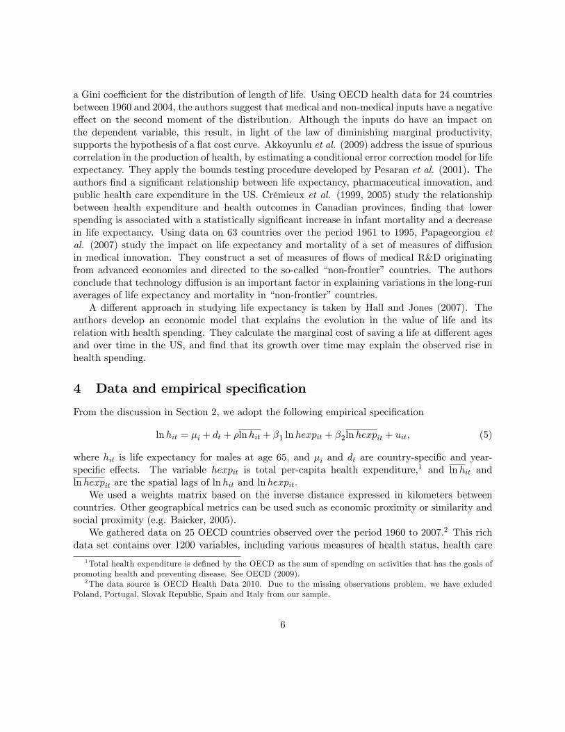
a Gini coe¢ cient for the distribution of length of life. Using OECD health data for 24 countriesbetween 1960 and 2004, the authors suggest that medical and non-medical inputs have a negativee¤ect on the second moment of the distribution. Although the inputs do have an impact onthe dependent variable, this result, in light of the law of diminishing marginal productivity,supports the hypothesis of a �at cost curve. Akkoyunlu et al. (2009) address the issue of spuriouscorrelation in the production of health, by estimating a conditional error correction model for lifeexpectancy. They apply the bounds testing procedure developed by Pesaran et al. (2001). Theauthors �nd a signi�cant relationship between life expectancy, pharmaceutical innovation, andpublic health care expenditure in the US. Crémieux et al. (1999, 2005) study the relationshipbetween health expenditure and health outcomes in Canadian provinces, �nding that lowerspending is associated with a statistically signi�cant increase in infant mortality and a decreasein life expectancy. Using data on 63 countries over the period 1961 to 1995, Papageorgiou etal. (2007) study the impact on life expectancy and mortality of a set of measures of di¤usionin medical innovation. They construct a set of measures of �ows of medical R&D originatingfrom advanced economies and directed to the so-called �non-frontier� countries. The authorsconclude that technology di¤usion is an important factor in explaining variations in the long-runaverages of life expectancy and mortality in �non-frontier�countries.

A di¤erent approach in studying life expectancy is taken by Hall and Jones (2007). Theauthors develop an economic model that explains the evolution in the value of life and itsrelation with health spending. They calculate the marginal cost of saving a life at di¤erent agesand over time in the US, and �nd that its growth over time may explain the observed rise inhealth spending.

4 Data and empirical speci�cation

From the discussion in Section 2, we adopt the following empirical speci�cation

lnhit = �i + dt + �lnhit + �1 lnhexpit + �2lnhexpit + uit; (5)

where hit is life expectancy for males at age 65, and �i and dt are country-speci�c and year-speci�c e¤ects. The variable hexpit is total per-capita health expenditure,1 and lnhit andlnhexpit are the spatial lags of lnhit and lnhexpit.

We used a weights matrix based on the inverse distance expressed in kilometers betweencountries. Other geographical metrics can be used such as economic proximity or similarity andsocial proximity (e.g. Baicker, 2005).

We gathered data on 25 OECD countries observed over the period 1960 to 2007.2 This richdata set contains over 1200 variables, including various measures of health status, health care

1Total health expenditure is de�ned by the OECD as the sum of spending on activities that has the goals ofpromoting health and preventing disease. See OECD (2009).

2The data source is OECD Health Data 2010. Due to the missing observations problem, we have exludedPoland, Portugal, Slovak Republic, Spain and Italy from our sample.

6

resources and utilization, health spending and �nancing. Drawing from this data, we incorporatein the regression a number of variables to control for di¤erences across countries and over timein lifestyles. Speci�cally, we consider three important variables related to lifestyle, given bydaily fat intake, alcohol and tobacco consumption (see Table 1 for a description). Further, weinclude social expenditure for old people, de�ned as all bene�ts and �nancial contributions tosupport the elderly during circumstances which adversely a¤ect their welfare. We note that thevariable social spending is only available for the years 1980 to 2005. Both health expenditureand social expenditure are expressed in per-capita terms and have been adjusted for purchasingpower parity. We recognize that other factors, such as body weight and education may a¤ect lifeexpectancy (Deaton and Paxon, 2001; Hendricks and Graves, 2009; Culter et al. 2006). However,for many countries, data on these additional variables are either not available or available for avery short time period.

Table 1 shows some descriptive statistics on the variables included in the model. We observethat our data set is highly unbalanced; in particular the sample size drops signi�cantly whenthe variable social expenditure is added to the regression.

Table 1: De�nition of variables and descriptive statistics

Variable Description Mean St. dev. N obs.

h N. of years 14.1 1.7 1,284

hexpPer-capita, in US$

at 2000 PPP rates1,605.4 905.4 935

fatGrammes per

capita per day119.4 28.6 1,183

tobaccoAnnual per capita

in grammes2,326.5 690.8 919

alcoholAnnual per capitain liters

10.0 3.9 1,241

socexpPer-capita, in US$

at 2000 PPP rates1,264.9 809.3 660

Notes: (�): per capita in this case means divided by population aged 15 years and over.

5 Empirical �ndings

Figure 1 shows life expectancy for males at age 65 in the OECD countries in 1960 and in 2007.During these years, life expectancy has increased markedly, rising from an average of 12.7 yearsin 1960 to 16.8 in 2007. That this measure of health outcome has risen greatly among developedcountries is well known, suggesting not only that greater numbers of individuals are reachingold age but also that elderly people are living longer (Jagger et al., 2008; Cutler et al., 2006).

7

Figure 1: Life expectancy at age 65 in the OECD countries in 1960 and 2007

However, it is important to observe that populations are not ageing uniformly in all nations.Australia and Japan experienced particular strong gains in life expectancy over time, placingthem at the top of the ranking in recent years. In contrast, countries from Eastern Europe,such as Hungary and the Slovak Republic show the lowest values for life expectancy throughoutthe sample period. According to the OECD (2009) health report, the gains in life expectancyregistered in the OECD countries can be explained in part by a marked reduction in death ratesfrom heart disease and celebro-vascular diseases (stroke) among elderly people.

Figure 2 reports the time series patterns of life expectancy for the OECD countries. Notethat, towards the end of the sample period, life expectancy patterns in most countries tend to getcloser. Only �ve countries diverge substantially from this trend and show a low life expectancythroughout the sample period. These are Hungary, Slovak Republic, Turkey, Poland and theCzech Republic. Later in the paper, we will test whether in the long-run countries tend toachieve similar levels of health outcomes.

Figure 3 shows the plot of the average life expectancy at age 65 and average health spendingacross countries for the period 1969 to 2007. As expected, both series trend up (as also con�rmedby our non-stationary tests reported in Table 4 below). Life expectancy shows a stable increaseover time, while health spending seems to rise more rapidly at the beginning and at the end ofour sample period.

8

Figure 2: Life expectancy at age 65 in the OECD countries over the period 1960-2007

1 2

1 3

1 4

1 5

1 6

1 7

1 9 6 9 1 9 7 8 1 9 8 7 1 9 9 6 2 0 0 5

V a lu e s   o f   L I F E E X P

5 0 0

1 0 0 0

1 5 0 0

2 0 0 0

2 5 0 0

V a lu e s   o f   H E A L T H E X P

L I F E E X P           &H E A L T H E X P

Figure 3: Life expectancy at age 65 and health spending over the period 1969-2007

9

Figure 4: Plot of the Moran statistic for the variable life expectancy at age 65 (in logs) in theOECD countries over the period 1969-2007

Figure 4 shows the standardized Moran statistic3 for the variable lnh in the OECD countriesfor the period 1969 to 2007. Note that all values of this statistic above the red line are statisticallysigni�cant at the 5 per cent signi�cance level. These results show a signi�cant Moran statisticfor the years 1980-1984 and from 1990 onwards. This initial exploratory analysis indicates thepresence of geographical concentration of the variable life expectancy at age 65, which will beincorporated in our empirical model. It is also suggested by the economic theory discussed inSection 2.

First, we discuss the estimation results of our production function using some observedmeasures of medical technology available at the country level. Table 2 presents a set of technologyvariables for the treatment of problems of the cardiovascular system, which are known to bethe leading cause of morbidity and mortality in older adults (OECD, 2009). These variablesare the number of percutaneous coronary interventions (PCI), the number of coronary bypassand stents placed on patients with cardiovascular problems, the number of daily doses of lipidmodifying and beta-blocking agents. We gathered these variables from the OECD Health Data2010.

The �rst two technologies have been used by Cutler and Huckman (2003) to study theimpact of technology di¤usion on health productivity in New York state. Moise (2003) hasalso studied the mechanisms of di¤usion of these procedures in the OECD countries, showing

3For each time period the Moran statistic has been standardized by using the moments of the empiricaldistribution generated by a random permutation procedure.

10

that the most important determinants of their utilization are GDP and hospital characteristicssuch as technology regulation and payment methods for hospitals and physicians. Coronarystents represent perhaps the most important improvement to PCI since the mid-1990s. Lipidmodifying and beta-blocking agents are drugs aimed at preventing and treating cardiovasculardisease (Dickson and Jacobzone, 2003). We note that bypass surgery, widely di¤used prior tothe early 1980s, is an invasive procedure that has been progressively substituted by the lesstraumatic coronary stents delivered percutaneously. With the exception of bypass surgery, thetechnology variables we have chosen have the characteristic of being minimally invasive and lesscostly than existing technologies for which they are often substitutes.

It is important to note that these technologies are only a subset of all possible technologiesthat may adopted to prevent, diagnose, and treat health problems for people aged over 65. Werefer to Comin and Hobijn (2009, 2010) for an extensive discussion of existing medical and non-medical technologies. Most of these variables are available only from 1990, and even then, onlyfor a few countries.4 Table 2 shows the number of observations per technology variable.

Table 2: Technology measures and their correlation with life expectancy and its spatial lag

Corr. with

Technology Description n.obs. lnh lnh

ln perc n. percutaneous coronary interv.(1) 285 0.281� 0.361�

ln bypass n. coronary bypass(1) 293 0.042 0.024

ln stent n. coronary stenting(1) 181 0.142� 0.199�

ln statin Cons. of lipid modifying agents (2) 189 0.740 0.887�

ln betabl Cons. of beta-blocking agents(2) 278 -0.045 0.247�

(1): expressed in n. procedures per 100,000 population (in-patients). (2): Expressed as n. of

de�ned daily doses (DDD) per 1,000 inhabitants. (�): Signi�cant at 5 per cent signi�cance level.

While aware of these data limitations, Table 3 explores the role in the production function ofeach technology separately, given that the presence of missing values prevented us from buildinga composite index of medical technology. The reported regressions do not include the spatiallags of life expectancy, due to their high correlation with the technology variables, as reportedin Table 2. Further, time dummies have not been included due to the little variation over timeof our variables, caused by data limitations. For comparison purposes, we also show a regressionwith no technology variables (see column I). Note that, when including our observed measuresof innovation, the sample size drops signi�cantly.

Under the classic FE speci�cation, health spending has a signi�cant impact on life ex-pectancy. All technologies except for coronary stents have a positive and signi�cant impact

4Before 1995, data on all these technology variables are available for no more than 9 countries.

11

on our health outcome. Further, the coe¢ cient attached to health spending is signi�cant, rang-ing from 0.059 when the variable measuring consumption of beta-blocking agents is included inthe regression, to 0.264 in the case of technology coronary stents. Again the latter number isbased on a fewer number of observations and should be interpreted with caution. Among thelifestyle variables, consumption of tobacco is statistically signi�cant with the correct sign in allregressions except for the one with Statin, where it is positive but insigni�cant. Consumptionof alcohol has a negative but statistically insigni�cant e¤ect on life expectancy in all regressionsexcept for the one with beta blockers, where it is negative and signi�cant. Fat intake has anegative and signi�cant e¤ect on life expectancy in the FE regression, but is positive and in-signi�cant in most technology variable regressions. Again this may be due to the number ofobservations lost due to the paucity of these technology variables.

Table 3: Estimation of the health production function including observed medical technology

Variables Coef. Std.err. Coef. Std.err. Coef. Std.err. Coef. Std.err. Coef. Std.err.

Technology:

ln perc 0.020� 0.005 - - - -

ln bypass - 0.017� 0.005 - - -

ln stent - - -0.002 0.003 - -

ln statin - - - 0.022� 0.009 -

ln betabl - - - - 0.050� 0.011

lnhexp 0.127� 0.028 0.119� 0.025 0.264� 0.036 0.172� 0.035 0.059� 0.024

ln tobacco -0.077� 0.017 -0.079� 0.019 -0.071� 0.021 0.006 0.029 -0.104� 0.019

ln alcohol -0.017 0.027 0.012 0.030 -0.030 0.034 -0.239 0.052 -0.056� 0.026

ln fat 0.032 0.050 0.009 0.051 0.017 0.050 0.254� 0.086 0.032 0.060

ln socsp 0.013 0.022 0.059� 0.019 -0.020 0.025 -0.016 0.045 0.082� 0.012

n. obs 139 146 77 83 146

Notes: individual �xed e¤ects have been included included. (�): Signi�cant at 5 per cent signi�cance level.

We now turn to the estimation of our production function keeping technology unobserved,as outlined in model (5). This allows us to expand the sample size considerably.

Our exploratory data analysis suggested that both life expectancy and health spending maybe non-stationary raising some concern on the validity of our OLS estimates (Engle and Granger,1987). Table 4 reports the Pesaran (2007) CIPS panel unit root tests on our variables. Thelow power of country by country test is one of the major motivation for the use of panel unitroot tests. A Monte Carlo exercise reported in Baltagi et al. (2007) has shown that CIPS testis quite robust to the presence of spatial dependence as explicitly modeled in our framework.The output provides evidence of non-stationarity for all variables, both when an intercept onlyis included in the speci�cation or when an intercept and a trend are included. The results are

12

obtained including 3 lags in the ADF regressions5. Non-stationarity of life expectancy is justi�edby the declining mortality pattern for the elderly. According to the UN-World Bank Populationdatabase, life expectancy on average for men at age 65 is likely to be 18.1 years in 2040 in theOECD countries (see also Hendricks and Graves, 2009).

Note that all variables except for fat intake and social expenditure for old people are station-ary when �rst di¤erences are applied. We have also computed a CIPS statistic for the spatial lagof the variable life expectancy, namely lnhit. Given the non-stationary nature of lnhit, we verifywhether applying the spatial operator may render the dependent variable stationary. However,the CIPS test does not reject the null hypothesis, thus indicating that lnhit is non-stationary.

Table 4: Panel unit root tests and cointegration analysis

CIPS panel unit root tests

Variables Intercept only Intercept and trendIn �rst di¤.

(interc. only)

lnh 1.287 0.693 -7.072�

lnh 1.252 -2.360� -13.709�

lnhexp 3.082 1.676 -3.029�

ln tobacco 1.572 3.100 -3.596�

ln alcohol 2.735 0.799 -8.054�

ln fat -0.447 0.873 -5.212�

ln socsp 5.456 2.361 -6.407�

(�): Signi�cant at 5 per cent signi�cance level.

Next, we checked whether our variables are cointegrated, by computing the Pedroni (1999)parametric group t-statistic to the residuals from a regression of life expectancy on its spatiallag and on the variables provided in Table 1. Table 5 reports the estimation of model (5) andthe Pedroni (1999) and Kao (1999) cointegration tests. As noted by Beenstock and Felsenstein(2010), if variables are cointegrated, the OLS estimator for regression parameters in (5) is super-consistent, regardless the endogeneity of the spatial lag lnhit appearing on the right hand side ofthe equation. For this reason, there is no need to use spatial techniques such as IV or ML, to dealwith the endogeneity of lnhit. We refer to Stock (1983) for further details on super-consistencyof the OLS estimator. As a further check, in Column (II) we report estimation of (5) also by theIV approach, where instruments are given by the spatial lags of the included regressors (Kelejianand Prucha, 1998), and the temporal lag of the spatial lag, namely �lnhit�1. Results show verysimilar coe¢ cients to the OLS estimates (Column I). Both Pedroni and Kao cointegration testsreported are signi�cant, suggesting the existence of a long-run economic relationship betweenhealth productivity, expenditure, the lifestyle variables and social spending for the elderly. In

5Some robustness checks show that the results reported do not change when varying the number of lagsincluded in the ADF regression.

13

the last column of Table 5 (Column (III)) we also report the dynamic �xed e¤ects estimatorof the long-run coe¢ cients and of the error correction term (Pesaran, Shin, and Smith, 1999).Results con�rm the signi�cant e¤ect of health spending on the dependent variable, as well as thepresence of a sizeable spatial e¤ect. Speci�cally, a one percentage increase in health spendinginduces a rise of 0.03-0.05 per cent in life expectancy on average. This corresponds to almost anextra half year of longevity. All risk factors show, as expected, a negative e¤ect on the dependentvariable. A rise of 1 per cent in annual tobacco per capita consumption implies a reduction inlife expectancy of around 0.04-0.06 per cent. This corresponds to over a half year reductionin longevity on average. As for fat intake, a 1 per cent increase in per capita consumptionreduces the dependent variable by 0.07-0.09 per cent. This is almost one additional year of lifeexpectancy, on average.

Table 5: Estimation of the health production function(I) Static FE (II) IV FE (III) Dynamic FE

Variables Coef. Std. err. Coef. Std. err. Coef. Std. err.

lnh 0.364� 0.159 0.360� 0.159 0.771� 0.279

lnhexp 0.032� 0.011 0.032� 0.011 0.051� 0.023

ln tobacco -0.046� 0.007 -0.045� 0.007 -0.063� 0.016

ln alcohol -0.010 0.010 -0.011 0.010 0.023 0.023

ln fat -0.073� 0.022 -0.071� 0.022 -0.098� 0.048

ln socsp 0.011� 0.006 0.010 0.006 -0.009 0.014

Error correction term - - - - -0.350� 0.040n.obs 426 425

Pedroni ADF group test -9.596� (0.00)

Kao test -2.347� (0.01)

Notes: Individual �xed e¤ects and time dummies are included.

(�): signi�cant at 5 per cent signi�cance level. p-values in parenthesis.

One may argue that life expectancy in a country is a¤ected not only by the current levelof resources deployed in the health sector, but also by what has been allocated in the past.Hence, as a robustness check we have also tried including in our regression the average of healthspending over a pre-speci�ed interval of time. Speci�cally, in (5) we have replaced lnhexpit withthe variable lnhexp�it =

Pns=0 lnhexpi;t�s, where we have set n equal to 4, 9 and then 14 years.

Results for the static �xed e¤ects estimation are reported in Table 6. Comparing these resultsto those in Table 5, the in�uence of health resources spent over a given period of time on lifeexpectancy is similar to the impact of current level of health resources.

14

Table 6: Estimation of the health production function using average health spending(I) n=4 (II) n=9 (III) n=14

Variables Coef. Std. err. Coef. Std. err. Coef. Std. err.

lnh�

0.359� 0.158 0.375� 0.159 0.358� 0.159

lnhexp 0.040� 0.012 0.031� 0.014 0.035� 0.014

ln tobacco -0.044� 0.007 -0.045� 0.007 -0.045� 0.007

ln alcohol -0.009 0.010 -0.007 0.010 -0.007 0.010

ln fat -0.071� 0.022 -0.078� 0.022 -0.083� 0.022

ln socsp 0.007 0.007 0.009 0.007 0.010 0.007

n.obs 435 437 437

Having established the existence of a cointegration relationship, we now turn to the estima-tion of the following error correction model

� lnhit = �i + dt + � (uit) + ��lnhit + 1� lnhexpit + 2�lnhexpit + "it; (6)

where in the parenthesis we have the previous period cointegration relation. The coe¢ cient �measures the speed of adjustment of life expectancy to a deviation from the long-run equilibriumrelation between the dependent variable and the regressors. Again, we estimate the above modelusing 30 countries followed over 49 years. For estimation, we adopt an IV approach, where,again, instruments are given by the spatial lags of the included regressors (Kelejian and Prucha,1998), and the temporal lag of the spatial lag, namely �lnhit�1. In this case, we drop from theregression lnhexpit as it is highly correlated with lnhit. Results are reported in Table 7. Thevariable health expenditure is statistically insigni�cant, suggesting that short-run adjustmentsin traditional input factors do not have an impact on health care productivity.6 There is alsofurther evidence of high degree of spatial correlation suggesting that the adoption of technologiesin a country is mostly driven by the adoption of the same technologies in neighbouring countries.While short-run adjustments in risk factors are statistically insigni�cant, �uctuations in socialexpenditure for the elderly seem to play a role in explaining life expectancy.

As previously observed in the descriptive data analysis, some Eastern European countries,at the beginning of our sample period are characterized by low life expectancies. We wish totest whether these countries in the long-run continue to experience low levels of life expectancy,

6We have also checked the sensitivity of our estimates by removing one country at a time from the sample. Thecoe¢ cient estimate of health spending varies very little. The only exception is when we remove the United States.In this case, the estimated coe¢ cient of health spending increases from 0.035 to 0.05 for the FE speci�cation. Thisindicates that the US exerts an in�uential set of observations in these regressions because the US is characterizedby low longevity accompained by high health expenditure levels (Preston and Ho, 2009).

15

Table 7: Error correction model (Engle and Granger two-step method)

Variables Coef. Std. err.

�lnhit 0.773� 0.147� lnhexpit 0.002 0.017� ln tobaccoit 0.007 0.017� ln alcoholit 0.000 0.009� ln fatit 0.013 0.021� ln socspit 0.016� 0.010ui;t�1 -0.028� 0.010

n.obs 324R2 0.142

Notes: Individual �xed e¤ects and time dummies are included. (�): signi�cant at 5 per cent signi�cance level.(+) use of bootstrapped standard errors.

or instead tend to catch up with the remaining countries. We do this by checking whether thereexists beta convergence in life expectancy in the OECD countries (Barro and Sala-i-Martin,1995). An empirical observation of beta convergence would suggest that countries tend toachieve similar levels of health outcomes in the long-run.

In order to do this, we regress the average growth rate of life expectancy over the pe-riod 1975 to 2006 on the initial level of life expectancy. Hence, our dependent variable is132 ln (hi;2006=hi;1975), while our key regressor is lnhi;1975. Due to the unbalancedness of the dataset, we focus only on 25 OECD countries. The results are reported in Table 8, Column (I). InColumn (II) we also control for health expenditure in the initial period, while in Column (III)we include the spatial lag of life expectancy in the initial period to control for technologicalinterdependence.

The estimated coe¢ cient of lnh1975 in Column (I) is negative and signi�cant, suggestingthat countries with a lower initial level of life expectancy have a faster health care growth thanthose with a higher initial level of life expectancy, and that they all converge to the same steadystate. A similar result is obtained when controlling for initial level of health spending, as wellas technological interdependence.

16

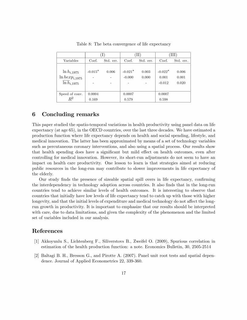
Table 8: The beta convergence of life expectancy

(I) (II) (III)Variables Coef. Std. err. Coef. Std. err. Coef. Std. err.

lnhi;1975 -0.015� 0.006 -0.021� 0.003 -0.022� 0.006

lnhexpi;1975 - - -0.000 0.000 0.001 0.001

lnhi;1975 - - - - -0.012 0.020

Speed of conv. 0.0004 0.0007 0.0007

R2 0.169 0.579 0.598

6 Concluding remarks

This paper studied the spatio-temporal variations in health productivity using panel data on lifeexpectancy (at age 65), in the OECD countries, over the last three decades. We have estimated aproduction function where life expectancy depends on health and social spending, lifestyle, andmedical innovation. The latter has been approximated by means of a set of technology variablessuch as percutaneous coronary interventions, and also using a spatial process. Our results showthat health spending does have a signi�cant but mild e¤ect on health outcomes, even aftercontrolling for medical innovation. However, its short-run adjustments do not seem to have animpact on health care productivity. One lesson to learn is that strategies aimed at reducingpublic resources in the long-run may contribute to slower improvements in life expectancy ofthe elderly.

Our study �nds the presence of sizeable spatial spill overs in life expectancy, con�rmingthe interdependency in technology adoption across countries. It also �nds that in the long-runcountries tend to achieve similar levels of health outcomes. It is interesting to observe thatcountries that initially have low levels of life expectancy tend to catch up with those with higherlongevity, and that the initial levels of expenditure and medical technology do not a¤ect the long-run growth in productivity. It is important to emphasize that our results should be interpretedwith care, due to data limitations, and given the complexity of the phenomenon and the limitedset of variables included in our analysis.

References

[1] Akkoyunlu S., Lichtenberg F., Siliverstovs B., Zweifel O. (2009), Spurious correlation inestimation of the health production function: a note. Economics Bulletin, 30, 2505-2514

[2] Baltagi B. H., Bresson G., and Pirotte A. (2007). Panel unit root tests and spatial depen-dence. Journal of Applied Econometrics 22, 339-360.

17

[3] Bai J., and Ng S. (2009), Boosting di¤usion indices. Journal of Applied Econometrics, 24,607-629.

[4] Baicker K (2005), The spillover e¤ects of state spending. Journal of Public Economics, 89,529-544

[5] Baicker K. and Chandra A., (2004), Medicare spending, The physician workforce, and thequality of health care received by Medicare bene�ciaries. Health A¤airs, 184-197.

[6] Barro R.J., and Sala-i-Martin X. (1995), Economic growth. New York, McGraw-Hill.

[7] Baumol W.J. (1967). Macroeconomics of unbalanced growth: the anatomy of urban crisis.American Economic Review, 57, 415-426.

[8] Birke D. (2009). The economics of networks: A survey of the empirical literature. Journalof Economic Surveys, 23, 762-793.

[9] Coleman J.S., Katz E. and Menzel H. (1966), Medical innovation: a di¤usion study. Inidi-anapolis, The Bobbs-Merril Company, Inc.

[10] Crémieux P.-Y., Ouellette P., Pilon C. (1999). Health care spending as determinants ofhealth outcomes. Health Economics, 8, 627-639.

[11] Crémieux P.-Y., Mieilleur M.-C., Ouellette P., Petit P., Zelder P., Potvin K. (2005), Publicand private pharmaceutical spending as determinants of health outcomes in Canada. HealthEconomics, 14, 107-116

[12] Comin D.A., and Hobijn B. (2010), An Exploration of Technology Di¤usion. AmericanEconomic Review, 100, 2031-2059

[13] Comin D.A., and Hobijn B. (2009), The CHAT dataset. NBER Working paper n. 15319.

[14] Cutler D.M., and Huckman R.S. (2003), Technological development and medical produc-tivity: the di¤usion of angioplasty in New York state. Journal of Health Economics. 22,187-217.

[15] Cutler D.M., Deaton A. S., Muney A. L (2006) The determinants of mortality. Journal ofEconomic Perspectives, 20, 97-120.

[16] Deaton A. and C. Paxon (2001) Mortality, Education, Income, and Inequality among Amer-ican Cohorts. University of Chicago Press.

[17] Dickson M., and Jacobzone S. (2003), Pharmaceutical Use and Expenditure for Cardiovas-cular Disease and Stroke: A Study of 12 OECD Countries. OECD Health Working papern.1.

18

[18] Engle, R.F., and Granger, C.W.J., (1987). Co-integration and error correction: Represen-tation, estimation and testing. Econometrica, 55, 251-276.

[19] Ertur C., Koch, W. (2007), Growth, technological interdependence and spatial externalities:Theory and evidence. Journal of Applied Econometrics. 22, 1033-1062.

[20] Fisher E.S., Bynum J.P., and Skinner J.S. (2009), Slowing the Growth of Health Care Costs- Lessons from Regional Variation. The New England Journal of Medicine, 360, 849-852.

[21] Fisher E.S., Wennberg D., Stukel T., Gottlieb D., Lucas F.L., and Pinder E.L. (2003),The implications of regional variations in Medicare spending Part 2: health outcomes andsatisfaction with Care. Annals of Internal Medicine, 138, 288-299.

[22] Frischer M. M. (2010), A spatial Mankiw-Romer-Weil model: theory and evidence. TheAnnals of Regional Science, forthcoming

[23] Greenwood J., Hercowitz Z. and Krussell P. (1997). Long-run implications of investment-speci�c technological change. American Economic Review, 87, 342-362.

[24] Grossman M. (1999). The human capital model of the demand for health. NBER WorkingPapers 7078, National Bureau of Economic Research.

[25] Hanada K. (1983) A formula of Gini�s concentration ratio and its application to life tables.Journal of Japan Statistical Society, 13, 95-98.

[26] Hendricks A. and P. E. Graves (2009) Predicting life expectancy: A cross country empiricalanalysis. Available at SSRN: http://ssrn.com/abstract=1477594

[27] Hall R. and Jones C. (2007), The value of life and the rise in health spending. The QuarterlyJournal of Economics, MIT Press, 122, 39-72.

[28] Jagger C., Gillies C., Moscone F., Cambois E., Van Oyen H., Nusselder W., Robine J.M., and the EHLEIS team, (2008), Inequalities in healthy life years in the 25 countries ofthe European Union in 2005: a cross-national meta-regression analysis. The Lancet, 372,2124-2131.

[29] Jones C. (2002), Why have health expenditures as a share of GDP risen so much?. NBERWorking Paper n. 9325.

[30] Kao, C. (1999), Spurious Regression and Residual-Based Tests for Cointegration in PanelData. Journal of Econometrics 90, 1-44.

[31] Kelejian H.H., Prucha I. (1998), A generalized spatial two-stage least squares procedure forestimating a spatial autoregressive model with autoregressive disturbances. Journal of RealEstate Finance and Economics, 17, 99-121.

19

[32] Keller W. (2004). Geographic localization of international technology di¤usion. AmericanEconomic Review 92, 120-142.

[33] Manski C. (1993) Identi�cation of endogenous social e¤ects: the reaction problem. Reviewof Economic Studies 60, 531-542.

[34] Moise P. (2003), The technology-health expenditure link a perspective from the ageing-related diseases study. In OECD (2003), A disease-based comparison of health systems:what is best and at what cost?.

[35] OECD (2009), Health at a glance 2009: OECD indicators.

[36] Papageorgiou C., Savvides A., Zachariadis M. (2007), International medical technologydi¤usion. Journal of International Economics, 72, 409-427.

[37] Pedroni P., (1999), Critical values for cointegration tests in heterogeneous panels withmultiple regressors, Oxford Bulletin of Economics and Statistics, 61, 653-670.

[38] Pesaran M. H., and Smith, R S. (1995) Estimating long-run relationships from dynamicheterogeneous panels, Journal of Econometrics 68, 79-113

[39] Pesaran M. H., Shin, Y. and Smith, R. J. (1999), Pooled mean group estimation of dynamicheterogenous panels. Journal of American Statistical Association, 94, 621-34.

[40] Pesaran M. H., Shin, Y. and Smith, R. J. (2001). Bounds testing approaches to the analysisof level relationships. Journal of Applied Econometrics, 16, 289-232.

[41] Preston S. H., and Ho J. Y. (2009), Low Life Expectancy in the United States: Is theHealth Care System at Fault?. PSC Working Paper Series PSC 09-03.

[42] Schoder J., Zweifel, P. (2009), Flat-of-the-curve medicine - a new perspective on the pro-duction of health. University of Zurich, Working Paper n. 0901.

[43] Shaw J. Horrace, W.,Vogel, R. (2005) The determinants of life expectancy: An analysis ofthe OECD health data. Southern Economic Journal, 71, 768-783.

[44] Skinner J., Fisher E., and Wennberg J.E. (2005), The E¢ ciency of Medicare in David Wise(ed.) Analyses in the Economics of Aging. Chicago: University of Chicago Press and NBER,129-157.

[45] Skinner J., Staiger D. (2009), Technology di¤usion and productivity growth in health care.NBER Working Paper n. 14865.

[46] Tu, J.V., et al. (1998), The fall and rise of carotid endarterectomy in the United States andCanada. The New England Journal of Medicine, 339, 1441-1447.

20

[47] Yusuf S., Peto R., Lewis J., Collins R., Sleight P. (1985), Beta blockade during and aftermyocardial infarction: an overview of the randomized trials. Progress in CardiovascularDiseases, 27, 335-371.

21