meeg source reconstruction: problems & solutions - … · 2012-05-03 · m/eeg source...

M/EEG source reconstruction:

problems & solutions

SPM-M/EEG course

Lyon, April 2012

C. Phillips, Cyclotron Research Centre, ULg, Belgium http://www.cyclotron.ulg.ac.be

Forward Problem

Inverse Problem

Source localisation in M/EEG

Head anatomy

Solution by Maxwell’s equations

Head model : conductivity layout Source model : current dipoles

Forward problem

t

EjB

t

BE

B

E

0

Ohm’s law :

Continuity equation :

Ej

tj

Maxwell’s equations (1873)

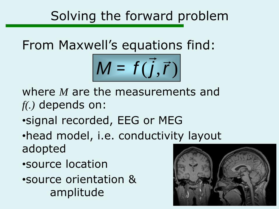
From Maxwell’s equations find:

where M are the measurements and f(.) depends on:

•signal recorded, EEG or MEG

•head model, i.e. conductivity layout adopted

•source location

•source orientation & amplitude

M = f ( j , r )

Solving the forward problem

From Maxwell’s equations find:

with f(.) as

•an analytical solution

- highly symmetrical geometry, e.g. spheres,

concentric spheres, etc.

- homogeneous isotropic conductivity

•a numerical solution

- more general (but still limited!) head model

M = f ( j , r )

Solving the forward problem

Con’s: •Human head is not spherical •Conductivity is not homogeneous and isotropic.

Analytical solution

Example: 3 concentric spheres

Pro’s: •Simple model •Exact mathematical solution •Fast calculation

Usually “Boundary Element Method” (BEM) : • Concentric sub-volumes of homogeneous and

isotropic conductivity,

• Estimate values on the interfaces.

Numerical solution

Pro’s: •More correct head shape modelling (not perfect though!)

Con’s: •Mathematical approximations of solution numerical errors

•Slow and intensive calculation

Features of forward solution

Find forward solution (any):

with f(.)

• linear in

• non-linear in

If N sources with known & fixed location,

then

M = f ( j , r )

j = jx jy jzéë ùû

T

r = rx ry rzéë ùû

T

M = f r1 r2… rN[ ]( ) × J = L × J

SPM solutions

Source space & head model

•Template Cortical Surface (TCS), in MNI space.

•Canonical Cortical Surface (CCS) = TCS warped to subject’s anatomy

•Subject’s Cortical Surface (SCS) = extracted from subject’s own structural image (BrainVisa/FreeSurfer)

SPM solutions

Jérémie Mattout, Richard N. Henson, and Karl J. Friston, 2007, Canonical Source Reconstruction for MEG

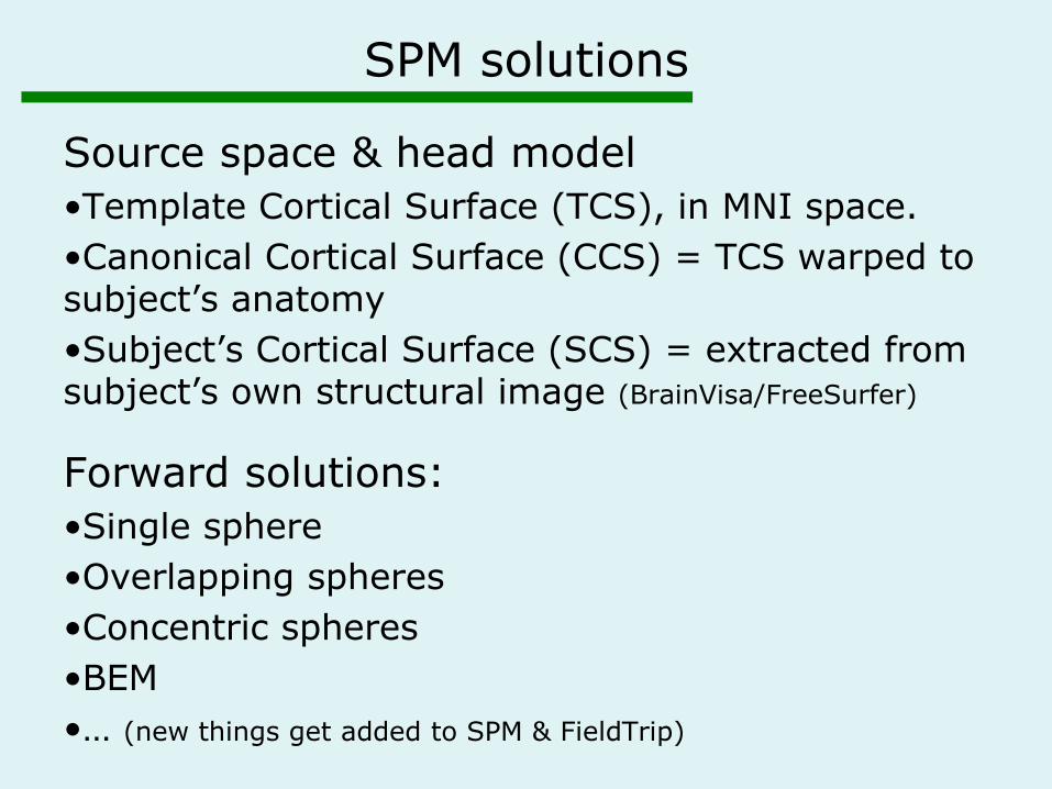
SPM solutions

Source space & head model

•Template Cortical Surface (TCS), in MNI space.

•Canonical Cortical Surface (CCS) = TCS warped to subject’s anatomy

•Subject’s Cortical Surface (SCS) = extracted from subject’s own structural image (BrainVisa/FreeSurfer)

Forward solutions:

•Single sphere

•Overlapping spheres

•Concentric spheres

•BEM

•… (new things get added to SPM & FieldTrip)

Forward Problem

Inverse Problem

Source localisation in M/EEG

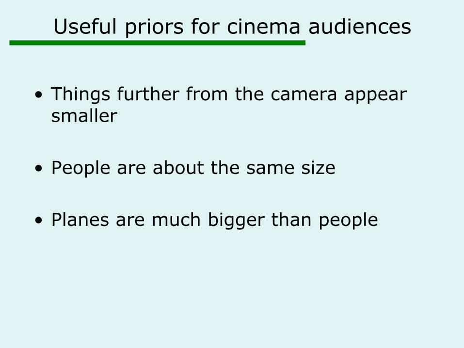
Useful priors for cinema audiences

• Things further from the camera appear smaller

• People are about the same size

• Planes are much bigger than people

M/EEG inverse problem

forward computation

Likelihood & Prior

inverse computation

Posterior & Evidence

p(Y |q, M ) p(q | M )

p(Y | M )p(q |Y, M )

Probabilistic framework

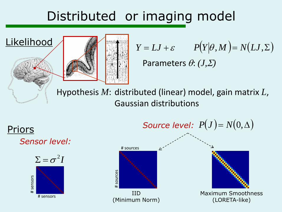
Distributed or imaging model

Likelihood ,, LJNMYP LJY

Hypothesis M: distributed (linear) model, gain matrix L, Gaussian distributions

Parameters : (J,)

Priors ,0NJP

Sensor level: # sources

# so

urc

es

IID (Minimum Norm)

Maximum Smoothness (LORETA-like)

Source level:

I2

# sensors

# se

nso

rs

The source covariance matrix

Source number

Sourc

e n

um

ber

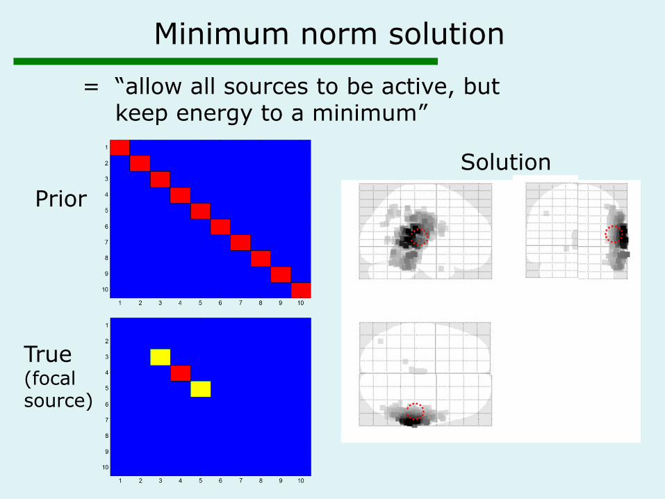
Minimum norm solution

Solution

0 100 200 300 400 500 600 700-10

-8

-6

-4

-2

0

2

4

6

8

10

estimated response - condition 1

at 52, -31, 11 mm

time ms

PPM at 379 ms (79 percent confidence)

512 dipoles

Percent variance explained 99.91 (93.65)

log-evidence = 21694116.2

0 100 200 300 400 500 600 700-10

-8

-6

-4

-2

0

2

4

6

8

10


at 52, -31, 11 mm

time ms


512 dipoles



Prior

True (focal source)

= “allow all sources to be active, but keep energy to a minimum”

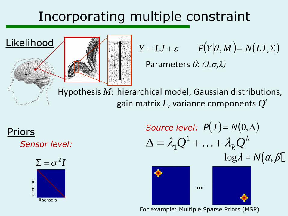
Incorporating multiple constraint

Likelihood ,, LJNMYP LJY

Hypothesis M: hierarchical model, Gaussian distributions, gain matrix L, variance components Qi

Parameters : (J,σ,λ)

Priors ,0NJP

Sensor level:

Source level:

I2

# sensors

# se

nso

rs

For example: Multiple Sparse Priors (MSP)

…

k

kQQ 1

1

logl = N a,b( )

0 100 200 300 400 500 600 700-8

-6

-4

-2

0

2

4

6

8


at 36, -18, -23 mm

time ms


512 dipoles



0 100 200 300 400 500 600 700-2

-1.5

-1

-0.5

0

0.5

1

1.5

2


at 46, -31, 4 mm

time ms


512 dipoles



0 100 200 300 400 500 600 700-2

-1.5

-1

-0.5

0

0.5

1

1.5

2


at 46, -31, 4 mm

time ms


512 dipoles



0 50 100 15010

2

104

106

108

Iteration

Free energy

Accuracy

Complexity

0 100 200 300 400 500 600 700-2

-1.5

-1

-0.5

0

0.5

1

1.5

2


at 46, -31, 4 mm

time ms


512 dipoles



Accuracy Free Energy Complexity

-6-4-20246x 1

0-1

3

-6

-4

-2

0

2

4

6

x 10-13

-6

-4

-2

0

2

4

6

x 10-13

Estimated data Estimated position

Measured data

?

Dipole fitting

Constraint: very few dipoles!

-6-4-20246x 1

0-1

3

-6

-4

-2

0

2

4

6

x 10-13

-6

-4

-2

0

2

4

6

x 10-13

Estimated data Prior source covariance

Measured data

?

Dipole fitting

True source covariance

Conclusion

• Solving the Forward Problem is not exciting but necessary…

…MEG or EEG? individual sMRI available? sensor location available?

• M/EEG inverse problem can be solved…

…If you provide some prior knowledge!

• All prior knowledge encapsulated in a covariance matrices (sensors & sources)

• Can test between models and priors (a.k.a. constraints) in a Bayesian framework.

Thank you for your attention

And many thanks to Gareth and Jérémie for the borrowed slides.

meeg source reconstruction: problems & solutions - … · 2012-05-03 · m/eeg source...

Documents