Melting Ice Caps: Implications for Asia-North AmericaLinkages and the Panama Canal

Joseph F. Francois1, Amanda M. Leister2, and Hugo Rojas-Romagosa*3

1University of Bern and CEPR2Colorado State University

3CPB Netherlands Bureau for Economic Policy Analysis

April 2015

AbstractArctic ice caps have been melting at an increased pace and projections im-

ply that the extent of the ice cover will be greatly reduced in the near future.Such a climatic phenomenon has important socio-economic implications, as itwould open up shipping routes in the Arctic. In this regard, media attentionand research has largely centered on the use of the Northern Sea Route (NSR)connecting Northeast Asia with Northwestern Europe and its effect on trafficthrough the Suez Canal. However, melting Arctic ice caps would also make theNorth West Route (NWR) a feasible trade route for high volume commercialtraffic, reducing the shipping distances between Northeast Asia and the EastCoast of the United States. In this paper we analyze the commercial feasi-bility of the NWR and the economic impact of reducing the trade distancesbetween Asia and the United States East Coast. In particular, we examine theextent to which the NWR would compete with the Panama Canal for certaintrade routes. Such competition has significant geopolitical implications linkedto both a drop in traffic through the Panama Canal as well as changes in theglobal supply chains that currently link East Asia and the United States.

Keywords: Arctic shipping routes, transportation costs, trade forecasting, grav-ity model, CGE models, trade and emissionsJEL Classification: R41, F17, C21, C68, D58, F18

1 IntroductionThe steady reduction of Arctic sea ice has been well documented (Rodrigues, 2008;Kinnard et al., 2011; Comiso, 2012). There is broad agreement on continued re-duction through the remainder of the century (Wang and Overland, 2009; Vavrus

*Corresponding author; e-mail: h.rojas-romagosa@cpb.nl

1

et al., 2012), and recent studies even suggest that the melting rate could accelerate(Kattsov et al., 2010; Rampal et al., 2011; Shepherd et al., 2012; Kerr, 2012; Stroeveet al., 2012; Slezak, 2013). Wang and Overland (2012) for example point to ice freeaccess to Arctic routes by the mid 2030s, while in a meta-analysis of model resultsRogers et al. (2015) identify a median prediction of 2034 for an ice free Arctic inSeptember. Stammerjohn et al. (2012) note that already, some Arctic routes areice free now more than predicted my climate models for 2030. This implies thateven in the near future, the extension of ice cover will be greatly reduced. Indeed asubstantial share of the Arctic may soon be completely ice-free for much of the year.

Besides the environmental effects, another consequence of this climatic phe-nomenon would be the viability of shipping routes in the Arctic. In this paper,we examine the economic effects of the viability of the North West Route (NWR)between Asia and North America for high volume commercial traffic. This route willreduce the shipping distances and time between Northeast Asia (i.e. China, Korea,Japan) and the East Coast of the United States and Canada (see Figure 1).

In this paper, we analyze the economic impact of the commercial feasibility ofthe NWR and realized reductions in the trade distances between Asia and NorthAmerica. With reduced ice cover the NWR becomes a direct competitor with thePanama Canal for certain trade routes. Such a change has significant geopoliticalimplications linked to both a drop in traffic through the Panama Canal as wellas changes in the global supply chains that currently link East Asia and NorthAmerica.1

Until 2011, there was still controversy about the feasibility of the commercial useof Arctic routes. However, the ever-quicker melting pace found in several studieshas broadened the consensus in favor of its likely commercial use in the near future.A growing number of papers find that both Arctic routes (i.e. the NSR and NWR)could be fully operational for several months or even all-year round in the nearfuture (cf. Verny and Grigentin, 2009; Liu and Kronbak, 2010; Khon et al., 2010;Stephenson et al., 2013; Wang and Overland, 2012; Rogers et al., 2015; Stammerjohnet al., 2012).2

Given current uncertainties regarding the relation between the icecap meltingpace and the transport logistic barriers associated with the NSR and the NWR,it is hard to predict the year when these new shipping routes will become fullyoperational. Throughout this paper we use a what-if approach where we assumethat by the year 2030 the icecaps have melted far enough and logistics issues relatedto navigating the Arctic have been resolved, so both the NSR and the NWR are

1In this way, this paper is a companion to Francois and Rojas-Romagosa (2015), with a focus onthe NSR. While we are concerned with the NWR here, throughout we assume that melting icecapswill allow the use of both the NSR and the NWR. The search for the NWR led to a great deal oftragedy, while motivating early exploration of much of the American interior and coasts. See forexample Berton (1988) on historic relevance, and Oestreng (1997) on geopolitical significance.

2The differences on the approximate year and the yearly extent for which the Arctic routes will befully operational varies much between papers, depending on different assumptions and estimationsregarding the pace of the ice caps melting and developments in the shipping industry with respectto the new route. More recent evidence points to accelerated loss of ice cover.

2

Figure 1: The North Western Route (NWR) and the Panama Canal shipping routes

fully operationally all year round.3 In practical terms, this also implies that we usean "upper bound" scenario that assumes that the NWR becomes a perfect substitutefor the Panama Canal, and as such, all commercial shipping between Northeast Asiaand the East coast of North America will use the shorter, faster, and cheaper NWRinstead of the Panama Canal route.4

Our economic analysis follows a three-step process. In the first step we esti-mate changes in physical distances between East Asia and the US along major andprospective shipping routes using both the NWR (new routes) and the PanamaCanal (current routes). The second step employs a regression-based gravity modelof trade to map the new distance calculations –for both the NWR and the PanamaCanal route– into estimates of the bilateral trade cost reductions between tradingpartners at the industry level. While part of this reduction in costs follows fromphysical shipping costs, other trade costs also follow from time and distance barri-

3The use of 2030 as our benchmark year is mainly for illustration purposes and the use of anotheryear does not affect our main economic results.

4Additionally, as in Francois and Rojas-Romagosa (2015) we assume that the NSR is a perfectsubstitute for the South Sea Route through the Suez Canal.

3

ers, as benchmarked in the gravity exercise. In the third step we integrate our tradecost reduction estimates into a computable general equilibrium (CGE) model of theglobal economy to simulate the effect of the commercial opening of both the NSRand NWR on bilateral trade flows, macroeconomic outcomes and the total amountof 𝐶𝑂2 emissions.5 It is important to note that since the opening of the Arctic ship-ping routes will be a gradual process that will take a number of years, the economicadjustment pattern we describe in our analysis will also be gradual.

The paper is organized as follows. In Section 2 we analyze logistic issues andprojections for commercially using Arctic routes, including the NSR and NWR, inthe future. We then explain how we estimate the new water-transportation distancesin Section 3 and then use these new distance measures to estimate the gravity modelof trade in Section 4. The CGE simulations and macroeconomic results are presentedin Section 5. We then compare our simulations results (using both the NSR andNWR) with the results found in Francois and Rojas-Romagosa (2015) where onlythe NSR was assumed to be used. Section 7 concludes by summarizing our mainresults.

2 Commercial feasibility of the Arctic shipping routesThere are two elements that condition the feasibility of Arctic routes (see Figure1) to become fully viable commercial substitutes of the current routes (SSR andPanama Canal). The first is the ice levels in the Arctic, which is the main barrierto the commercial use of the NSR and NWR. A quicker melting pace will makethe commercial use of the NWR more likely in the near future. Figure 2 furtherillustrates the current degree of ice cap melting (until 2012).

The second barrier to the Arctic routes is the transport logistic issues associatedwith the opening of new commercial shipping routes in regions without transportinfrastructure and extreme weather conditions. Even though a number of ships havealready used the NSR and the NWR during summer months, significant logisticalobstacles remain. These include slower speeds, limited commercial weather forecasts,patchy search and rescue capabilities, scarcity of relief ports along the route and theneed to use icebreakers and/or ice-capable vessels (Liu and Kronbak, 2010; Schøyenand Bråthen, 2011). These conditions not only affect the insurance premia currentlycharged to use the Arctic routes, but also limit the commercial viability of shippingoperations, which are dependent on predictability, punctuality and economies ofscale (Humpert and Raspotnik, 2012).

Moreover, Stephenson et al. (2013) estimate that the NWR has a substantiallower prospect of full-year navigation than the NSR. Khon et al. (2010) find that:"The models predict prolongation of the season with a free passage from 3 to 6

5In practical terms, we build on the results of Francois and Rojas-Romagosa (2015), mappingthese into transport and trade cost reductions associated along the SSR through the Panama canaland the NWR and focusing in the impact on trade-related linkages between North America andAsia.

4

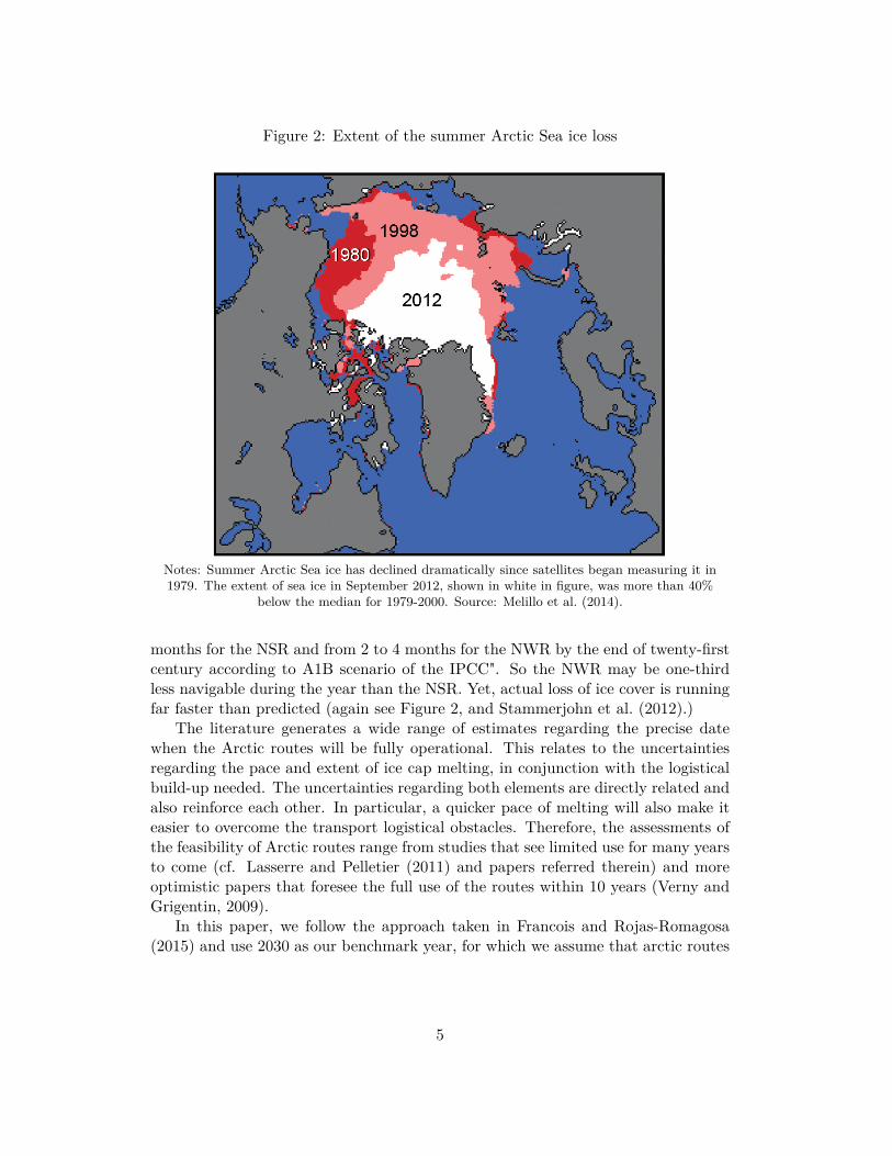
Figure 2: Extent of the summer Arctic Sea ice loss

Notes: Summer Arctic Sea ice has declined dramatically since satellites began measuring it in1979. The extent of sea ice in September 2012, shown in white in figure, was more than 40%

below the median for 1979-2000. Source: Melillo et al. (2014).

months for the NSR and from 2 to 4 months for the NWR by the end of twenty-firstcentury according to A1B scenario of the IPCC". So the NWR may be one-thirdless navigable during the year than the NSR. Yet, actual loss of ice cover is runningfar faster than predicted (again see Figure 2, and Stammerjohn et al. (2012).)

The literature generates a wide range of estimates regarding the precise datewhen the Arctic routes will be fully operational. This relates to the uncertaintiesregarding the pace and extent of ice cap melting, in conjunction with the logisticalbuild-up needed. The uncertainties regarding both elements are directly related andalso reinforce each other. In particular, a quicker pace of melting will also make iteasier to overcome the transport logistical obstacles. Therefore, the assessments ofthe feasibility of Arctic routes range from studies that see limited use for many yearsto come (cf. Lasserre and Pelletier (2011) and papers referred therein) and moreoptimistic papers that foresee the full use of the routes within 10 years (Verny andGrigentin, 2009).

In this paper, we follow the approach taken in Francois and Rojas-Romagosa(2015) and use 2030 as our benchmark year, for which we assume that arctic routes

5

will be fully operational all-year round.6 This implies that we use an "upper bound"scenario that estimates the largest expected trade and economic impact from theArctic routes. For instance, if the routes are not operational during winter and/orother logistic issues related to the extreme weather of the Arctic are not fully re-solved, then it can be expected that shipping companies pursue a diversificationstrategy, using both routes conditional on which offers the lowest costs at certainseasons the year.7

3 Estimating US trade distance reductions using theNorth Western Route

As the first step of our analysis, we estimate the precise distance reductions forbilateral trade flows associated with the NWR. To do so we include shipping routes inthe estimation of the distance between two trading partners in the gravity equation.8Sea transport is the most important transport mode for global trade: 90 percent ofworld trade is carried by ship (OECD, 2011). The rest moves primarily by land.9 Forthe country pairs and trade flows we focus on in this research, water transportation,or multi-modal transport (water and land) accounts for essentially all trade.

Therefore, we use the actual shipping distances collected in Francois and Rojas-Romagosa (2015).10 The more challenging issue is to assess the impact of the NWRon US international trade. As a large country with major ports in both the Atlanticand Pacific oceans, the US has a variety of trade routes that link it with NortheastAsia (i.e. China, Japan and Korea). From the data collected in Francois and Rojas-Romagosa (2015) we have shipping distances for three US ports: Newark (NewJersey), New Orleans (Louisiana) and Long Beach (California).

6However, our economic estimations are not dependent on this occurring precisely in 2030. Wechose a benchmark year mainly for reporting reasons, since we expect to have quantitatively similarresults if we used another benchmark year, either an earlier one (2015) or later one (2040). FromFrancois and Rojas-Romagosa (2015) we know that the use of different benchmark years affects thesize of some of the results, but the main qualitative results and patterns for 2030 remain robust tothe use of different years.

7Another potential limitation is the increased pressure on current transportation infrastructure.In particular, current shipping hubs may need to expand. However, since the opening of the NSRand NWR will be a gradual process, we expect that any additional infrastructure needs can bedeveloped while the Arctic routes become fully operational.

8Currently, the econometric literature on the gravity model of bilateral trade relies on measures ofphysical distances between national capitals as a measure of distance, known as the CEPII database(Mayer and Zignago, 2011). However, these measures use the shortest physical distance and thus,are not appropriate for our work, since shipping routes are usually longer than the shortest physicaldistance, and melting sea ice, for example, will not change the physical distance between Tokyo andNew York.

9Very few exceptions use air transportation, which mainly applies for high-value commoditiesthat need to reach the final destination in a short time (e.g. fish and flowers).

10This paper provides a detailed explanation on how the shipping distances are constructed. Inessence, the distances are constructed using shipping industry data on the physical distance betweenports. For landlocked countries, we combine the port-to-port distances with land-transport distancesfrom the CEPII’s database.

6

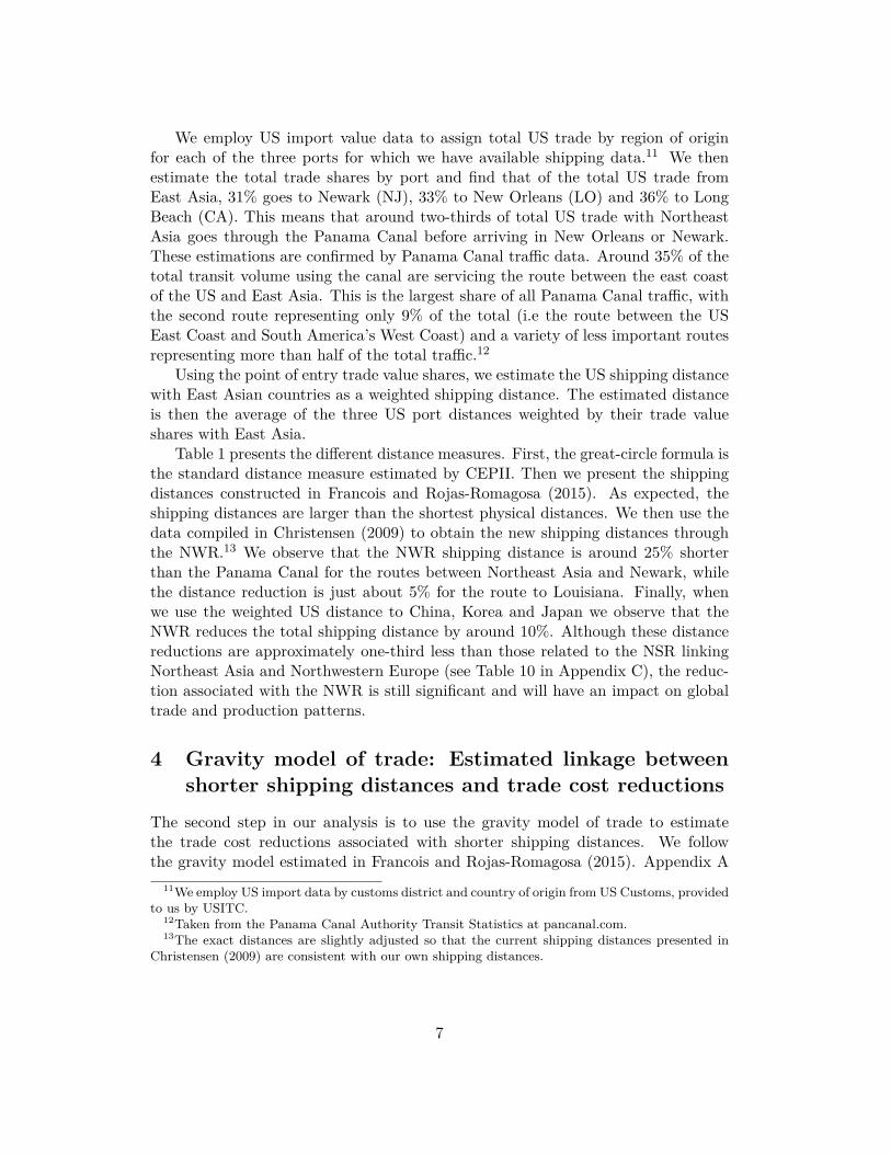
We employ US import value data to assign total US trade by region of originfor each of the three ports for which we have available shipping data.11 We thenestimate the total trade shares by port and find that of the total US trade fromEast Asia, 31% goes to Newark (NJ), 33% to New Orleans (LO) and 36% to LongBeach (CA). This means that around two-thirds of total US trade with NortheastAsia goes through the Panama Canal before arriving in New Orleans or Newark.These estimations are confirmed by Panama Canal traffic data. Around 35% of thetotal transit volume using the canal are servicing the route between the east coastof the US and East Asia. This is the largest share of all Panama Canal traffic, withthe second route representing only 9% of the total (i.e the route between the USEast Coast and South America’s West Coast) and a variety of less important routesrepresenting more than half of the total traffic.12

Using the point of entry trade value shares, we estimate the US shipping distancewith East Asian countries as a weighted shipping distance. The estimated distanceis then the average of the three US port distances weighted by their trade valueshares with East Asia.

Table 1 presents the different distance measures. First, the great-circle formula isthe standard distance measure estimated by CEPII. Then we present the shippingdistances constructed in Francois and Rojas-Romagosa (2015). As expected, theshipping distances are larger than the shortest physical distances. We then use thedata compiled in Christensen (2009) to obtain the new shipping distances throughthe NWR.13 We observe that the NWR shipping distance is around 25% shorterthan the Panama Canal for the routes between Northeast Asia and Newark, whilethe distance reduction is just about 5% for the route to Louisiana. Finally, whenwe use the weighted US distance to China, Korea and Japan we observe that theNWR reduces the total shipping distance by around 10%. Although these distancereductions are approximately one-third less than those related to the NSR linkingNortheast Asia and Northwestern Europe (see Table 10 in Appendix C), the reduc-tion associated with the NWR is still significant and will have an impact on globaltrade and production patterns.

4 Gravity model of trade: Estimated linkage betweenshorter shipping distances and trade cost reductions

The second step in our analysis is to use the gravity model of trade to estimatethe trade cost reductions associated with shorter shipping distances. We followthe gravity model estimated in Francois and Rojas-Romagosa (2015). Appendix A

11We employ US import data by customs district and country of origin from US Customs, providedto us by USITC.

12Taken from the Panama Canal Authority Transit Statistics at pancanal.com.13The exact distances are slightly adjusted so that the current shipping distances presented in

Christensen (2009) are consistent with our own shipping distances.

7

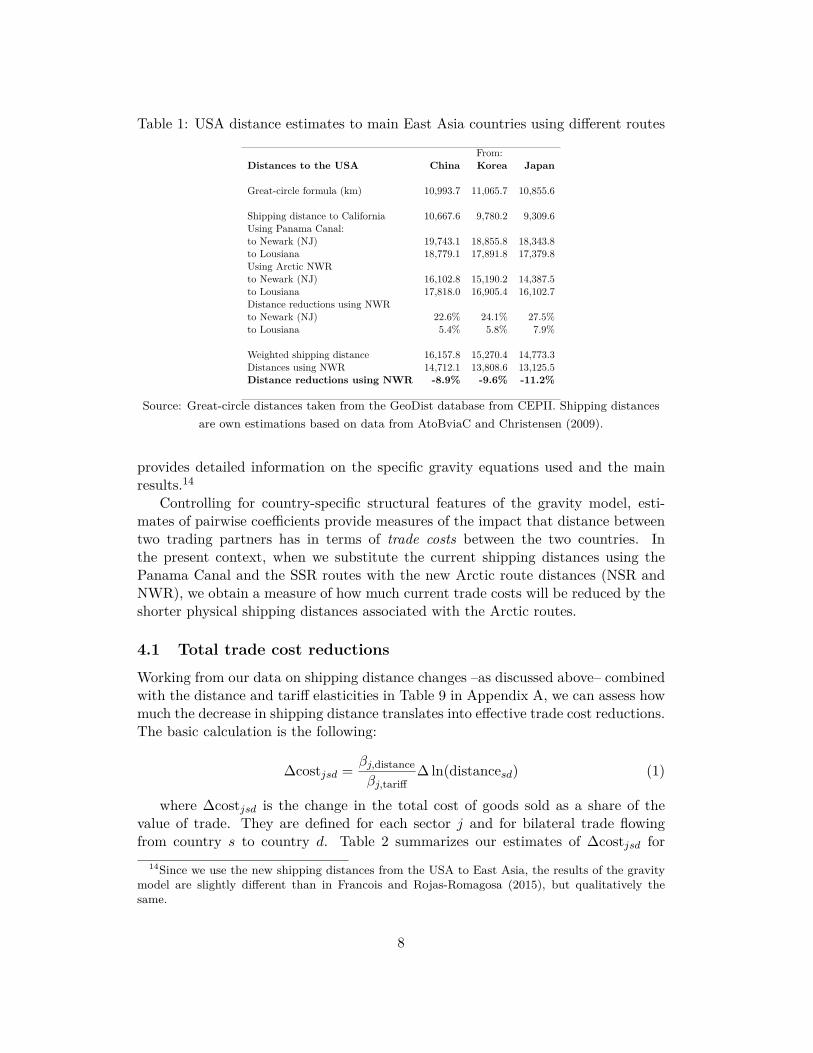
Table 1: USA distance estimates to main East Asia countries using different routes

From:Distances to the USA China Korea Japan

Great-circle formula (km) 10,993.7 11,065.7 10,855.6

Shipping distance to California 10,667.6 9,780.2 9,309.6Using Panama Canal:to Newark (NJ) 19,743.1 18,855.8 18,343.8to Lousiana 18,779.1 17,891.8 17,379.8Using Arctic NWRto Newark (NJ) 16,102.8 15,190.2 14,387.5to Lousiana 17,818.0 16,905.4 16,102.7Distance reductions using NWRto Newark (NJ) 22.6% 24.1% 27.5%to Lousiana 5.4% 5.8% 7.9%

Weighted shipping distance 16,157.8 15,270.4 14,773.3Distances using NWR 14,712.1 13,808.6 13,125.5Distance reductions using NWR -8.9% -9.6% -11.2%

Source: Great-circle distances taken from the GeoDist database from CEPII. Shipping distancesare own estimations based on data from AtoBviaC and Christensen (2009).

provides detailed information on the specific gravity equations used and the mainresults.14

Controlling for country-specific structural features of the gravity model, esti-mates of pairwise coefficients provide measures of the impact that distance betweentwo trading partners has in terms of trade costs between the two countries. Inthe present context, when we substitute the current shipping distances using thePanama Canal and the SSR routes with the new Arctic route distances (NSR andNWR), we obtain a measure of how much current trade costs will be reduced by theshorter physical shipping distances associated with the Arctic routes.

4.1 Total trade cost reductions

Working from our data on shipping distance changes –as discussed above– combinedwith the distance and tariff elasticities in Table 9 in Appendix A, we can assess howmuch the decrease in shipping distance translates into effective trade cost reductions.The basic calculation is the following:

Δcost𝑗𝑠𝑑 = 𝛽𝑗,distance𝛽𝑗,tariff

Δ ln(distance𝑠𝑑) (1)

where Δcost𝑗𝑠𝑑 is the change in the total cost of goods sold as a share of thevalue of trade. They are defined for each sector 𝑗 and for bilateral trade flowingfrom country 𝑠 to country 𝑑. Table 2 summarizes our estimates of Δcost𝑗𝑠𝑑 for

14Since we use the new shipping distances from the USA to East Asia, the results of the gravitymodel are slightly different than in Francois and Rojas-Romagosa (2015), but qualitatively thesame.

8

both the NWR (above) and the NSR (below). Note that these total trade costs aresector-specific and are not symmetric for country pairs. For instance, the trade costsfrom USA to Korea are slightly different than from Korea to the USA. As expected,since the distance changes associated with the NWR are one-third lower than theNSR changes, the related trade cost reductions are also smaller for the NWR.

Table 2: Total trade cost reductions for the Arctic routes between 20 non-servicessectors for selected countries, percentage changes.

trade cost reductions trade cost reductionsFrom: To: average max min From: To: average max min

NWR route:USA CHN 1.03 3.15 0.08 CHN USA 1.03 3.15 0.08USA JPN 1.30 3.97 0.11 JPN USA 1.30 3.96 0.11USA KOR 1.11 3.39 0.09 KOR USA 1.10 3.38 0.09USA TWN 0.77 2.36 0.06 TWN USA 0.77 2.36 0.06

NSR route:DEU CHN 3.51 10.39 0.30 CHN DEU 3.50 10.35 0.30DEU JPN 5.24 15.33 0.46 JPN DEU 5.22 15.28 0.46DEU KOR 4.22 12.45 0.37 KOR DEU 4.21 12.41 0.37DEU TWN 2.39 7.13 0.21 TWN DEU 2.38 7.11 0.20

Notes: Average is the mean trade cost reductions between all 20 sectors, while max and min arethe maximum and minimum trade cost reductions, respectively. Source: Own estimations.

4.2 Cost allocation between transport services and other tradecosts

To link our gravity estimations with the CGE model, we allocate these total tradecost reductions from Equation (1) over actual international transport services costs("atall" in the GTAP code) and the remainder as iceberg trade cost reductions ("ams"in the GTAP code).

We first estimate the shipping services costs reduction as the percentage distancereduction associated with the Arctic routes:

atall𝑠𝑑 = −(︂NSR/NWRdistance𝑠𝑑

distance𝑠𝑑− 1

)︂(2)

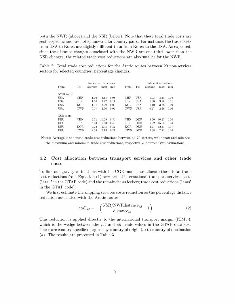
This reduction is applied directly to the international transport margin (ITM𝑠𝑑),which is the wedge between the fob and cif trade values in the GTAP database.These are country specific margins: by country of origin (𝑠) to country of destination(𝑑). The results are presented in Table 3.

9

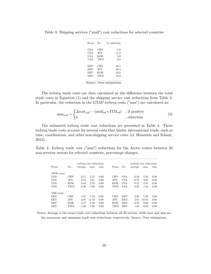
Table 3: Shipping services ("atall") cost reductions for selected countries

From: To: % reduction

USA CHN 8.9USA JPN 11.2USA KOR 9.6USA TWN 6.8

DEU CHN 28.1DEU JPN 39.4DEU KOR 33.0DEU TWN 19.9

Source: Own estimations.

The iceberg trade costs are then calculated as the difference between the totaltrade costs in Equation (1) and the shipping service cost reductions from Table 3.In particular, the reduction in the GTAP iceberg costs ("ams") are calculated as:

ams𝑗𝑠𝑑 ={︃

Δcost𝑗𝑠𝑑 − (atall𝑠𝑑 * ITM𝑠𝑑) , if positive0 , otherwise

(3)

The estimated iceberg trade cost reductions are presented in Table 4. Theseiceberg trade costs account for several costs that hinder international trade, such astime, coordination, and other non-shipping service costs (cf. Hummels and Schaur,2012).

Table 4: Iceberg trade cost ("ams") reductions for the Arctic routes between 20non-services sectors for selected countries, percentage changes.

iceberg cost reductions iceberg cost reductionsFrom: To: average max min From: To: average max min

NWR routeUSA CHN 0.51 2.47 0.00 CHN USA 0.49 2.43 0.00USA JPN 0.45 2.91 0.00 JPN USA 0.75 3.05 0.00USA KOR 0.44 2.52 0.00 KOR USA 0.55 2.47 0.00USA TWN 0.30 1.60 0.00 TWN USA 0.35 1.84 0.00

NSR routeDEU CHN 1.87 7.54 0.00 CHN DEU 2.00 7.56 0.00DEU JPN 3.07 11.52 0.00 JPN DEU 2.63 10.73 0.00DEU KOR 2.17 8.30 0.00 KOR DEU 2.76 9.98 0.00DEU TWN 1.36 4.90 0.00 TWN DEU 1.38 6.02 0.00

Notes: Average is the mean trade cost reductions between all 20 sectors, while max and min arethe maximum and minimum trade cost reductions, respectively. Source: Own estimations.

10

5 CGE analysis of trade and macroeconomic outcomesThe trade cost estimates described previously are integrated into a computable gen-eral equilibrium (CGE) model of the global economy in our third and final step. Theopening and future use of the NWR and the NSR will have a simultaneous effecton multiple countries and will influence how different trading partners interact withone another. The use of the Arctic routes will have several impacts, including tradefacilitation that will affect bilateral trade, as well as sectoral production and con-sumption patterns, relative domestic and international prices, and how the regionand sector-specific factors of production (i.e. labor and capital) are used. Accord-ingly, we employ a CGE modeling framework that is widely used and accepted forthe study of global economic shocks to the international trading system and wellsuited for this analysis.15 The primary advantages of the CGE modeling frameworkinclude the analysis of how key variables will respond to changes in trade coststhat we estimate, given the future use of the NWR. The CGE framework beginsby creating a baseline scenario of the global economy in the year 2030 based onmacroeconomic projections and comparing how the projected 2030 economy wouldrespond to changes in trade costs. This allows for the quantification of resultingchanges in bilateral trade flows, relative prices and corresponding changes in pro-duction and consumption throughout the global economy, as well as changes in 𝐶𝑂2emissions that may arise given global economic adjustments to the opening of theArctic routes. The opening of the NSR and NWR, therefore, fits within the analyt-ical scope of CGE models since it implies a very seizable shock to the world tradesystem that will affect a large set of countries simultaneously.16

The particular CGE model we use is a modified version of a standard GTAPclass CGE model. The model characteristics are detailed in Appendix B.17 Onekey specification that is pertinent to our analysis of the NWR is the calculation ofchanges in 𝐶𝑂2 emissions by region and sector, given the emergence of new traderoutes and corresponding changes in production. The inclusion of 𝐶𝑂2 data and themodel-predicted changes in 𝐶𝑂2 emissions allow for the analysis of environmentalimpacts that are expected, given the future use of the NWR. We use the GTAPglobal database that describes the initial equilibrium of the economy, includes com-plete bilateral trade information, as well as transport and protection linkages, and

15See for instance, Schmalensee et al. (1998), Elliott et al. (2010), Peng (2011); Beckman et al.(2011); Boehringer et al. (2011); Böhringer et al. (2012); Auffhammer and Steinhauser (2012); Dixonand Jorgenson (2013).

16We recognize the importance of recent quantitative trade models –summarized by Costinot andRodríguez-Clare (2013)– yet these models are not able to account for the economic shocks resultingfrom the opening of the Arctic routes. Further discussion is provided in Appendix B.

17The main distinction between our model and the standard GTAP model is that we use amonopolistic competition framework with increasing returns to scale (�̀� la Krugman, 1980), and𝐶𝑂2 emissions are directly linked to production, consumption and trade. The model is implementedin GEMPACK under OSX and the model code is available upon request, as well as an executableversion of the model.

11

parameters that define elasticities for supply and demand.18 The current versionof the database includes data for 129 regions and 57 sectors for the year 2007 thatwe thoughtfully aggregated to describe the 39 regions and 23 sectors of most im-portance for this research (see Table 11 and Table 12 in Appendix C). To assessthe global general equilibrium effects of the commercial use of the NWR, we projectthe database along the medium or SSP2 (Shared Socioeconomic Pathway) from themost recent SSPs and related Integrated Assessment scenarios (IIASA, 2012; O’Neillet al., 2012). Our work focuses on the year 2030 from this baseline.19 Our modelingframework allows us to assess both the trade and macroeconomic implications as-sociated with the NWR, as well as changes in 𝐶𝑂2 emissions from production andinternational transport.

Working from the 2030 projection along the baseline SSP, we report our mainCGE results as the differences between the baseline values in 2030 (i.e. the base-line scenario with no Arctic shipping lanes) compared to the counterfactual scenariowhere bilateral trade is permitted to move through the NSR and NWR. The NWRscenario incorporates both the transportation and trade cost reductions that we esti-mate into our CGE model to assess the impacts of the Arctic routes on bilateral tradeflows, sectoral output, and other macroeconomic variables.20 Our work explicitlyaccounts for the input-output relationships within countries and sectors embodied inglobal value chains (GVC). This allows for the assessment of how GVC may adjustto the NWR that creates new shipping distances and corresponding cost reductions.Furthermore, we quantify impacts of the NWR on welfare and employment/wagechanges. Finally, we quantify the effects of the NWR on transportation relatedpollution levels that considers both distance reductions as well as the potential forlarger trade volumes.

5.1 Trade effects

The global and bilateral trade changes resulting from the NWR scenario that allowsfor the NSR and NWR to be fully operational are relative to the baseline 2030scenario that is in absence of the Arctic shipping lanes as a viable trade route. Ourresults show that utilization of the Arctic routes will reduce international shipping,volume by distance, by 0.71%, and that the corresponding volume of global tradeincreases by 0.76%. While values for global trade volumes are relatively modest, it isimportant to note that concentration of trade that is affected is primarily centeredon trade changes between Northeast Asia (i.e. China, Japan and South Korea),Europe, and the east coast of the United States. Our estimates for the share of

18GTAP is the standard basic dataset used in most CGE models. See Narayanan et al. (2012)for documentation on the GTAPv8 database and Hertel (2013) for the full database project.

19Robustness checks that assess impacts given other years for which the NWR is fully operational,indicate that while magnitudes of the relative trade effects (which depend on projected GDP growth)differ, the main results found for 2030 are not significantly different.

20As explained in Section 4, we accomplish this by implementing technical efficiency gains inshipping and iceberg trade costs that are equivalent to the estimated reductions in total tradecosts.

12

world trade that will now flow through the Arctic routes, rather than traditionalroutes, is equal to 13.5%.

In this "upper bound" scenario, where the NWR is a perfect substitute for thePanama Canal, the increase in the trade between the US East Coast and NortheastAsia implies that both the current Panama Canal traffic that serves both regions(around 35% of the total canal traffic, see Section 3), but also the increased tradewill be using the NWR. Employing current data from the Panama Canal Authorityon the number of vessels that use the canal, we estimate that approximately between4000 to 4500 vessels will be using the NWR (instead of the Panama Canal) when itis fully operational all-year round.21

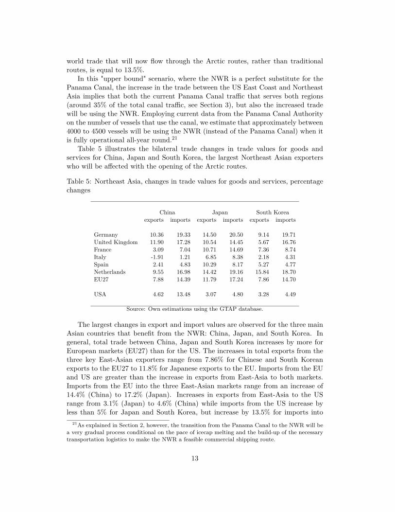
Table 5 illustrates the bilateral trade changes in trade values for goods andservices for China, Japan and South Korea, the largest Northeast Asian exporterswho will be affected with the opening of the Arctic routes.

Table 5: Northeast Asia, changes in trade values for goods and services, percentagechanges

China Japan South Koreaexports imports exports imports exports imports

Germany 10.36 19.33 14.50 20.50 9.14 19.71United Kingdom 11.90 17.28 10.54 14.45 5.67 16.76France 3.09 7.04 10.71 14.69 7.36 8.74Italy -1.91 1.21 6.85 8.38 2.18 4.31Spain 2.41 4.83 10.29 8.17 5.27 4.77Netherlands 9.55 16.98 14.42 19.16 15.84 18.70EU27 7.88 14.39 11.79 17.24 7.86 14.70

USA 4.62 13.48 3.07 4.80 3.28 4.49

Source: Own estimations using the GTAP database.

The largest changes in export and import values are observed for the three mainAsian countries that benefit from the NWR: China, Japan, and South Korea. Ingeneral, total trade between China, Japan and South Korea increases by more forEuropean markets (EU27) than for the US. The increases in total exports from thethree key East-Asian exporters range from 7.86% for Chinese and South Koreanexports to the EU27 to 11.8% for Japanese exports to the EU. Imports from the EUand US are greater than the increase in exports from East-Asia to both markets.Imports from the EU into the three East-Asian markets range from an increase of14.4% (China) to 17.2% (Japan). Increases in exports from East-Asia to the USrange from 3.1% (Japan) to 4.6% (China) while imports from the US increase byless than 5% for Japan and South Korea, but increase by 13.5% for imports into

21As explained in Section 2, however, the transition from the Panama Canal to the NWR will bea very gradual process conditional on the pace of icecap melting and the build-up of the necessarytransportation logistics to make the NWR a feasible commercial shipping route.

13

China. Table 13 in Appendix C includes the corresponding data for merchandisetrade in volumes, which exhibits a similar pattern to the changes in trade valuesdescribed above.

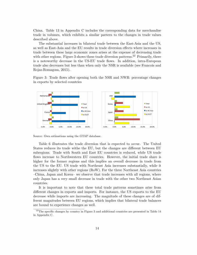
The substantial increases in bilateral trade between the East-Asia and the US,as well as East-Asia and the EU results in trade diversion effects where increases intrade between these large economic zones arises at the expense of decreasing tradewith other regions. Figure 3 shows these trade diversion patterns.22 Primarily, thereis a noteworthy decrease in the US-EU trade flows. In addition, intra-Europeantrade also decreases but less than when only the NSR is available (see Francois andRojas-Romagosa, 2015).

Figure 3: Trade flows after opening both the NSR and NWR: percentage changesin exports by selected countries

-­‐5.0%   0.0%   5.0%   10.0%   15.0%   20.0%  

Germany  

France  

United  Kingdom  

Netherlands  

Total  

to  US  

to  NE  Asia  

to  EU27  

-­‐5.0%   0.0%   5.0%   10.0%   15.0%   20.0%  

China  

Japan  

Korea  

USA  

Total  

to  US  

to  NE  Asia  

to  EU27  

Source: Own estimations using the GTAP database.

Table 6 illustrates the trade diversion that is expected to occur. The UnitedStates reduces its trade withe the EU, but the changes are different between EUsubregions. Trade with South and East EU countries is reduced, while US tradeflows increase to Northwestern EU countries. However, the initial trade share ishigher for the former regions and this implies an overall decrease in trade fromthe US to the EU. US trade with Northeast Asia increases substantially, while itincreases slightly with other regions (RoW). For the three Northeast Asia countries–China, Japan and Korea– we observe that trade increases with all regions, whereonly Japan has a very small decrease in trade with the other two Northeast Asiancountries.

It is important to note that these total trade patterns sometimes arise fromdifferent changes in exports and imports. For instance, the US exports to the EUdecrease while imports are increasing. The magnitude of these changes are of dif-ferent magnitudes between EU regions, which implies that bilateral trade balancesare bound to experience changes as well.

22The specific changes by country in Figure 3 and additional countries are presented in Table 14in Appendix C.

14

Table 6: Changes in trade values by region for selected countries, percentage changes

USA China Japan Koreaexports imports trade exports imports trade exports imports trade exports imports trade

Total EU -1.6 0.3 -0.6 7.8 14.0 9.0 11.7 16.9 13.6 8.1 14.7 10.4South EU -0.8 -0.1 -0.4 -0.2 3.1 0.5 6.8 7.5 7.1 3.1 3.9 3.4

East EU -2.9 0.4 -1.2 9.5 18.3 11.3 10.7 17.9 12.3 7.8 16.3 8.7NW EU 6.1 2.8 4.2 8.4 14.7 9.6 4.7 3.4 4.0 2.8 2.4 2.6NE Asia 11.3 4.1 7.0 -0.2 0.7 0.2 -0.1 -0.1 -0.1 0.7 -0.2 0.2

USA 0.0 0.0 0.0 4.6 13.5 8.1 3.1 4.8 3.7 3.3 4.5 3.9RoW -0.5 1.4 0.5 0.9 2.0 1.4 0.5 0.7 0.6 0.3 0.8 0.6

TOTAL 2.7 2.2 2.4 2.0 2.5 2.2 1.6 1.4 1.5 1.3 1.2 1.3

Notes: South EU is: Cyprus, Greece, Italy, Malta, Portugal and Spain. East EU is: Bulgaria,Czech Republic, Estonia, Hungary, Latvia, Lithuania, Poland, Romania, Slovakia and Slovenia.Northwestern (NW) EU is: Austria, Belgium, Denmark, Finland, France, Germany, Ireland,Luxembourg, the Netherlands, Sweden and the United Kingdom. Northeast (NE) Asia is: China,Japan, South Korea, Hong Kong and Taiwan. RoW is Rest of the World.Source: Own estimations using the GTAP database.

Similar trade diversion patterns persist when considering expected exports atthe sectoral level. Tables 15 and 16 in Appendix C illustrate changes in exports tothe US and China by sector. Changes in sectoral exports are evenly spread amongall manufacturing sectors with few exceptions (mainly the service sectors). Table15 illustrates the percentage changes in export sales to the US. Results indicatethat China, Japan and South Korea significantly increase their exports to the USin almost all sectors but services (Japanese exports of wood products and transportservices may decreases as well). However, European countries decrease their exportsto the US for the majority of sectors, with exceptions in four sectors being potentialincreases in exports of agricultural products, plant products, petrochemicals andgas, and mining and extraction.

Given substantial trade diversion for key economic players in the global mar-ket, the expected changes in aggregate exports are minor, with the largest increaseexpected for the US at 2.7% (see Figure 4). After the US, China experiences thelargest overall export increase at 2%, followed by Japan and Korea. Within the EU,the Northwestern countries increase exports (Germany, United Kingdom and theNetherlands), with a slight increase in France and Spain, and an export decrease inItaly. Total World exports increase at 0.76%.

5.2 Macroeconomic outcomes

Resulting macroeconomic effects given changes in trade flows show countries thatbenefit from the opening of Arctic routes as well as countries that are worse off froma macroeconomic standpoint (see Figure 5). GDP and welfare, measured as thepercentage changes in per capita utility, are expected to increases slightly (less than0.25%) for some Northwestern European countries (Germany, United Kingdom, theNetherlands) as well as minor increases in Japan (0.25%) and the largest gains ex-

15

Figure 4: Changes in export values by selected countries, percentage changes

-­‐0.5  

0  

0.5  

1  

1.5  

2  

2.5  

3  

FRA   DEU   ITA   NLD   ESP   GBR   CHN   JPN   KOR   USA   World  

Source: Own estimations using the GTAP database.

pected for China and South Korea (1% and 0.75%, respectively).23 Welfare and GDPgains are negligible for the US and relatively minor (less than -0.25%, in general) forFrance and Spain, while Italy has the largest welfare losses at -0.36%. These welfarelosses are attributable to the disruption in intra-EU trade and regional productionvalue chains resulting from the opening of the Arctic routes. While the macroe-conomic effects of trade diversion may seem relatively minor, the GDP changesexpected from the opening of the Arctic routes is comparable to estimates of GDPchanges for key global trade liberalization from a potential Doha agreement withinthe WTO, or a potential bilateral Transatlantic Trade and Investment Partnershipagreement between the US and EU.24

Figure 6 illustrates that there is a direct relationship between the expected realincome changes and the corresponding country-specific changes in exports (and over-all trade volumes). In general, countries that increase their exports are those thatalso benefit from the opening of the Arctic routes.

5.3 Labor market effects

We investigate the effects on labor by employing two different CGE model closures.The baseline scenario for which we have presented results thus far, assumes a flex-

23See also Table 17 in Appendix C for the GDP and real income changes for all countries. Wealso include two measures of changes in welfare: per capita utility and equivalent variation (EV)in US$ million. Both welfare measures follow roughly the same pattern as GDP and real incomechanges.

24See for example Francois (2000), Francois et al. (2005), and Francois et al. (2013b)).

16

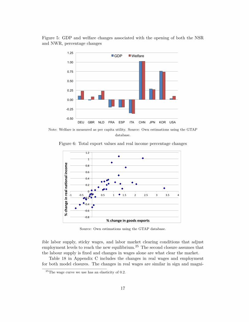
Figure 5: GDP and welfare changes associated with the opening of both the NSRand NWR, percentage changes

-0.50

-0.25

0.00

0.25

0.50

0.75

1.00

1.25

DEU GBR NLD FRA ESP ITA CHN JPN KOR USA

GDP Welfare

Note: Welfare is measured as per capita utility. Source: Own estimations using the GTAPdatabase.

Figure 6: Total export values and real income percentage changes

-­‐0.8  

-­‐0.6  

-­‐0.4  

-­‐0.2  

0  

0.2  

0.4  

0.6  

0.8  

1  

1.2  

-­‐1   -­‐0.5   0   0.5   1   1.5   2   2.5   3   3.5   4  

%  cha

nge  in  re

al  na,

onal  income  

%  change  in  goods  exports  

Source: Own estimations using the GTAP database.

ible labor supply, sticky wages, and labor market clearing conditions that adjustemployment levels to reach the new equilibrium.25 The second closure assumes thatthe labour supply is fixed and changes in wages alone are what clear the market.

Table 18 in Appendix C includes the changes in real wages and employmentfor both model closures. The changes in real wages are similar in sign and magni-

25The wage curve we use has an elasticity of 0.2.

17

tude for both closures that we employ. Furthermore, the expected changes in realwages follow a similar pattern as the real income changes. In general, the countrieswith expected declines in real incomes also have expected decreases in real wages.Furthermore, this pattern extends to the results for both skilled and unskilled la-bor, indicating that the expected changes in the relative demand for skilled andunskilled workers are minimal.26 For instance, the US experiences changes in wagesand employment that are very close to zero: between -0.05% and -0.01%.

The changes in total employment are negligible, as illustrated by Table 18 inAppendix C being less than a tenth of a percentage point. For most countries, thechanges in real wages are not large enough to affect the overall labor supply. Underthe assumption of a fixed labor supply, no changes are expected in employment byconstruction, as wages adjust to maintain full employment levels.

Results for the changes in employment do vary by sector, as shown in Table 19in Appendix C. We create a labor displacement indicator to further describe thesectoral changes in employment, which is equal to the weighted standard deviationof the changes in employment by sector. This allows for a standardized measureof the employment changes by country. While there is variation by country for thelabor that is displaced to another sector, these changes are around 1% on average forthe labor force in a given country. The US, for example, has a labor displacementvalue of just around 0.35 for unskilled labor and 0.25 for skilled labor.

Furthermore, Table 19 also shows the country-specific percentage changes forunskilled workers in four selected sectors. The changes in employment of unskilledworkers vary by country and sector and can be relatively high, especially in someEuropean countries, reaching more than a 14% decrease in employment in the othermanufactures sector for four countries in Europe. While the expected changes inlabor displacement can be quite substantial in certain sectors, the adjustments inproduction and employment are expected to occur gradually over time in responseto the speed by which the Arctic routes replace traditional transportation routes.

5.4 Changes in 𝐶𝑂2 emissions

Changes in trade flows given the emergence of Arctic shipping routes may lead tothe assumption that fuel costs and 𝐶𝑂2 emissions would decrease for the watertransportation sector, given shorter shipping distances between trading partners.However, the increases in trade volumes resulting from the decreased shipping dis-tances between Northeastern Asia and Europe and the east coast of North Americacauses increased demand for shipping services. Consequently, the decreased dis-tance is largely offset by the increased demand for shipping for regions that benefitmost from the opening of the Arctic routes. Results show minimal decreases in𝐶𝑂2 emissions for most countries, yet slight increases in emissions for Northeast

26These results are as expected, given the relatively small changes in sectoral output. The demandfor skill levels differ by sector; however, if output shares by sector do not vary significantly, thecorresponding demand for workers of different skill levels and the skill premium (the differencebetween skilled and unskilled wages) will remain steady.

18

Asian countries. Overall, there is a minor increase in estimated global 𝐶𝑂2 emis-sions equal to 12.46 million MT which is an increase of 0.02% relative to baselineemission levels (see Table 20 in Appendix C).27 It is important to recognize thatwe assume constant emission levels by sector and country, meaning that there areno technological advancements or new policy changes altering emission levels (i.e.carbon taxes, emission permits) by country and sector for both the baseline andArctic routes counter-factual.

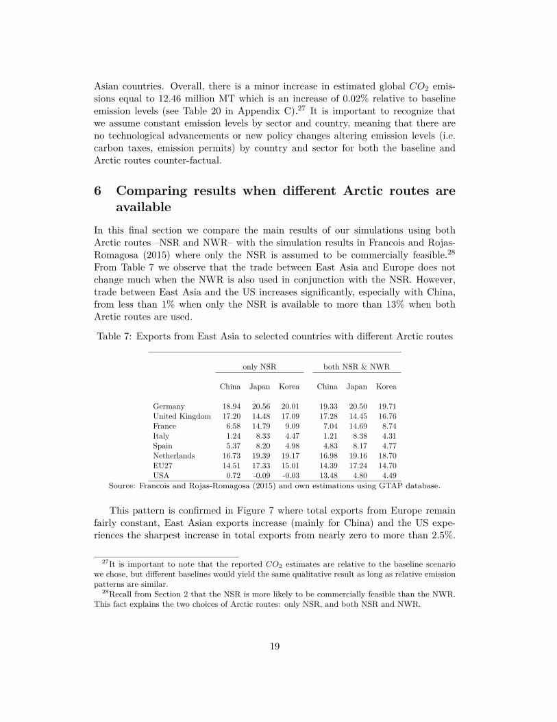
6 Comparing results when different Arctic routes areavailable

In this final section we compare the main results of our simulations using bothArctic routes –NSR and NWR– with the simulation results in Francois and Rojas-Romagosa (2015) where only the NSR is assumed to be commercially feasible.28

From Table 7 we observe that the trade between East Asia and Europe does notchange much when the NWR is also used in conjunction with the NSR. However,trade between East Asia and the US increases significantly, especially with China,from less than 1% when only the NSR is available to more than 13% when bothArctic routes are used.

Table 7: Exports from East Asia to selected countries with different Arctic routes

only NSR both NSR & NWR

China Japan Korea China Japan Korea

Germany 18.94 20.56 20.01 19.33 20.50 19.71United Kingdom 17.20 14.48 17.09 17.28 14.45 16.76France 6.58 14.79 9.09 7.04 14.69 8.74Italy 1.24 8.33 4.47 1.21 8.38 4.31Spain 5.37 8.20 4.98 4.83 8.17 4.77Netherlands 16.73 19.39 19.17 16.98 19.16 18.70EU27 14.51 17.33 15.01 14.39 17.24 14.70USA 0.72 -0.09 -0.03 13.48 4.80 4.49

Source: Francois and Rojas-Romagosa (2015) and own estimations using GTAP database.

This pattern is confirmed in Figure 7 where total exports from Europe remainfairly constant, East Asian exports increase (mainly for China) and the US expe-riences the sharpest increase in total exports from nearly zero to more than 2.5%.

27It is important to note that the reported 𝐶𝑂2 estimates are relative to the baseline scenariowe chose, but different baselines would yield the same qualitative result as long as relative emissionpatterns are similar.

28Recall from Section 2 that the NSR is more likely to be commercially feasible than the NWR.This fact explains the two choices of Arctic routes: only NSR, and both NSR and NWR.

19

Figure 7: Total exports for selected countries using different Arctic routes, percent-age changes

-1.0

-0.5

0.0

0.5

1.0

1.5

2.0

2.5

3.0

DEU GBR FRA ITA ESP NLD CHN JPN KOR USA

only NSR both NSR & NWR

Source: Francois and Rojas-Romagosa (2015) and own estimations using the GTAP database.

Export changes are translated into GDP and welfare (i.e. per capita utility)effects. The US moves from negative to positive GDP and welfare changes, whileChina experiences a doubling on both variables. This relatively big increases areassociated with the baseline scenario where China is the country with the largestgrowth rate, and as such, has more capacity to expand exports and take advantageof both Arctic routes. On the contrary, Japan and Korea do not experience muchchanges from the first scenario to the second in which the NWR is also commerciallyfeasible. For Europe, the changes from one scenario to the other are also small, butin general the positive and negative effects are reduced, because trade diversionthrough the NSR only, is less intensive with the opening of the NWR: East Asiaexports more to the US in this second case.

Table 8: GDP and welfare changes associated with different Arctic routes

only NSR both NSR & NWR

GDP Welfare GDP Welfare

Germany 0.18 0.32 0.10 0.11United Kingdom 0.01 0.10 -0.01 -0.05France -0.25 -0.22 -0.20 -0.23Italy -0.51 -0.52 -0.35 -0.37Spain -0.27 -0.25 -0.20 -0.26Netherlands 0.21 0.32 0.12 0.15China 0.57 0.56 1.02 1.13Japan 0.29 0.27 0.29 0.36Korea 0.73 0.70 0.76 0.78United States -0.03 -0.04 0.03 0.08

Source: Francois and Rojas-Romagosa (2015) and own estimations using GTAP database.

20

Finally, in Table 21 in Appendix C we observe that 𝐶𝑂2 emissions are increasingfor both scenarios, but the increase is smaller for the case where both the NSR andNWR are used. This is explained by the emission reductions in the US (using theshorter NWR than the Panama Canal) that compensates for the increased emissionsfrom China, which is expanding its exports using both Arctic routes.

7 SummaryContinued melting of the Arctic ice caps is expected to allow the commercial feasi-bility of the Northern Sea Route and the North Western Route. Use of the Arcticshipping lanes would significantly reduce shipping distances and travel times be-tween Northeast Asia and two of the world’s largest economies, the EU and US,which will create opportunities for growth in trade between these critical regions.US Customs data shows that two thirds of US trade with Northeastern Asia travelsthrough the Panama Canal, which represents 35% of the ship traffic through thecanal. The distance reductions between the US and key Northeast Asian countriesgiven use of the NWR rather than the Panama Canal range from 9% to 11% whichcorresponds to estimated shipping services cost reductions ranging from nearly 7%to more than 11% from the US and from 20% to 40% from Western Europe toNortheast Asian countries.

Therefore, if the NWR becomes a full-year commercially feasible route betweenEast Asia and North America, it is then expected that the current commercialtraffic that goes through the Panama Canal will be reduced by up to one-third andbetween 4000 and 4500 vessels will be using the NWR. These shipping route changeswill generate massive geopolitical implications for both Panama and Canada (wheremost of the NWR is located). Nevertheless, the transition from the Panama Canalto the NWR will be a very gradual process conditional on the pace of icecap melting.

The decreased distances, transportation and trade cost reductions associatedwith both Arctic routes are expected to increase trade flows between Northeast Asiaand the US by values ranging from 3.1% to nearly 13.5%, and increases in NortheastAsia-EU trade between 7.9% to 17.2%, depending on bilateral trade partners. Thesetrade increases are translated into improvements in welfare and GDP growth in thecountries that experience the biggest exports changes from the opening of the Arcticroutes. In particular, China, Japan and Korea will benefit the most from these newshipping routes.

There are minor increases in 𝐶𝑂2 emissions expected, given increased globaltrade volumes and corresponding changes in region and sector-specific production.This undoubtedly raises additional questions regarding the environmental impactsof potential future commercial use of the Arctic routes as viable shipping lanes. Fur-thermore, trade diversion effects will negatively impact some (Central and Southern)European countries that suffer from decreases in intra-European trade, as well aspotential labor displacement given production responses that are region and sectorspecific.

21

Overall, Northeast Asian countries, the US and a subset of European countriesstand to benefit from commercial use of Arctic shipping lanes. When we comparetwo Arctic shipping scenarios –i.e. only the NSR is available, and both the NSRand NWR are used– the main difference is that the US will experience a significantexport increase and a move from negative to positive GDP and welfare increases.China is expected to benefit the most from the joint use of both Arctic routes.

Environmental and socio-political concerns, however, may affect the degree towhich these emerging trade routes may be utilized in the future. Above all, thedegree to which these emerging trade routes are viable shipping options depend onthe future condition of the Arctic icecaps and the ability of the shipping indus-try to overcome transport logistic issues that will allow the routes to become fullyoperational.

Acknowledgements

We deeply appreciate Marinos Tsigas and David Lundy (both from USITC) forproviding us with the district-specific US trade data.

ReferencesAnderson, J. E. and E. van Wincoop (2003). “Gravity with Gravitas: A Solution to

the Border Puzzle,” American Economic Review, 93(1), 170–192.

Anderson, J. E. and Y. Yotov (2012). “Gold Standard Gravity,” NBER WorkingPaper 17835.

Arkolakis, C., A. Costinot, and A. Rodríguez-Clare (2012). “New Trade Models,Same Old Gains?” American Economic Review, 102(1), 94–130.

Auffhammer, M. and R. Steinhauser (2012). “Forecasting the Path of US CO2 Emis-sions Using State-Level Information,” Review of Economics and Statistics, 94(1),172–185.

Baldwin, R. E. and D. Taglioni (2006). “Gravity for Dummies and Dummies forGravity Equations,” NBER Working Paper 12516.

Beckman, J., T. Hertel, and W. Tyner (2011). “Validating Energy-oriented CGEModels,” Energy Economics, 33, 799–806.

Berton, P. (1988). The Arctic Grail: The Quest for the Northwest Passage and TheNorth Pole, 1818-1909, Toronto: McClelland & Stewart.

Boehringer, C., J. C. Carbone, and T. F. Rutherford. (2011). “Embodied CarbonTariffs,” NBER Working Paper 17376.

22

Böhringer, C., E. J. Balistreri, and T. F. Rutherford. (2012). “The Role of BorderCarbon Adjustment in Unilateral Climate Policy: Overview of an Energy Model-ing Forum Study (EMF 29),” Energy Economics, 34, S97–S110.

Christensen, S. A. (2009). “Are the Northern Sea Routes Really the Shortest?” DIISBrief March, Danish Institute for International Studies (DIIS).

Comiso, J. C. (2012). “Large Decadal Decline of the Arctic Multiyear Ice Cover,”Journal of Climate, 25(4), 1176–1193.

Costinot, A. and A. Rodríguez-Clare (2013). “Trade Theory with Numbers: Quan-tifying the Consequences of Globalization,” in Handbook of International Eco-nomics, ed. by G. Gopinath, E. Helpman, and K. Rogoff, North Holland, vol. 4.

De Benedictis, L. and L. Tajoli (2011). “The World Trade Network,” World Econ-omy, 34(8), 1417–1454.

Dixon, P. and D. Jorgenson, eds. (2013). Handbook of Computable General Equilib-rium Modeling, vol. 1, Elsevier: North Holland.

Dür, A., L. Baccini, and M. Elsig (2014). “The Design of International Trade Agree-ments: Introducing a New Database,” Review of International Organizations,Forthcoming.

Easley, D. and J. Kleinberg (2010). Networks, Crowds, and Markets: Reasoningabout a Highly Connected World, Cambridge, UK: Cambridge University Press.

Eaton, J. and S. Kortum (2002). “Technology, Geography and Trade,” Econometrica,70(5), 1741–1779.

Egger, P., M. Larch, K. E. Staub, and R. Winkelmann (2011). “The Trade Effects ofEndogenous Preferential Trade Agreements,” American Economic Journal: Eco-nomic Policy, 3(3), 113–143.

Elliott, J., I. Foster, S. Kortum, T. Munson, F. Perez Cervantes, and D. Weisbach(2010). “Trade and Carbon Taxes,” American Economic Review, 100(2), 465–469.

Francois, J. F. (2000). “Assessing the Results of General Equilibrium Studies ofMultilateral Trade Negotiations,” Working paper, UNCTAD, Geneva.

Francois, J. F., M. Manchin, and W. Martin (2013a). “Market Structure in Multisec-tor General Equilibrium Models of Open Economies,” in Handbook of ComputableGeneral Equilibrium Modeling, ed. by P. Dixon and D. Jorgenson, Amsterdam:Elsevier.

Francois, J. F., M. Manchin, H. Norberg, O. Pindyuk, and P. Tomberger (2013b).“Reducing Trans-Atlantic Barriers to Trade and Investment,” Final project report,Centre for Economic Policy Research (CEPR), London.

23

Francois, J. F. and D. Nelson (2002). “A Geometry of Specialization,” EconomicJournal, 112(481), 649–678.

Francois, J. F. and H. Rojas-Romagosa (2015). “Melting Ice Caps and the Eco-nomic Impact of Opening the Northern Sea Route,” CPB Discussion Paper, CPBNetherlands Bureau for Economic Policy Analysis.

Francois, J. F. and D. Roland-Holst (1997). “Scale Economies and Imperfect Com-petition,” in Applied Methods for Trade Policy Analysis: A Handbook, ed. by J. F.Francois and K. A. Reinert, Cambridge: Cambridge University Press, 331–362.

Francois, J. F., H. van Mijl, and F. van Tongeren (2005). “The Doha Round andDeveloping Countries,” Economic Policy, 20(42), 349–391.

Francois, J. F. and J. Woerz (2009). “Non-linear Panel Estimation of Import Quotas:The Evolution of Quota Premiums Under the ATC,” Journal of InternationalEconomics, 78(2), 181–191.

Hertel, T. (2013). “Global Applied General Equilibrium Analysis Using the GlobalTrade Analysis Project Framework,” in Handbook of Computable General Equilib-rium Modeling, ed. by P. Dixon and D. Jorgenson, Amsterdam: Elsevier: NorthHolland.

Hummels, D. and G. Schaur (2012). “Time as a Trade Barrier,” NBER WorkingPaper 17758.

Humpert, M. and A. Raspotnik (2012). “The Future of Arctic Shipping,” Port Tech-nology International, 55, 10–11.

IIASA (2012). “Supplementary Note for the SSP Data Sets,” Database and docu-mentation SSP2, International Institute for Applied Systems Analysis (IIASA).

Kattsov, V. M., V. E. Ryabinin, J. E. Overland, M. C. Serreze, M. Visbeck, J. E.Walsh, W. Meier, and X. Zhang (2010). “Arctic Sea Ice Change: A Grand Chal-lenge of Climate Science,” Journal of Glaciology, 56, 1115–1121.

Kerr, R. A. (2012). “Experts Agree Global Warming Is Melting the World Rapidly,”Science, 338, 1138.

Khon, V., I. I. Mokhov, M. Latif, V. A. Semenov, and W. Park (2010). “Perspec-tives of Northern Sea Route and Northwest Passage in the Twenty-first Century,”Climate Change, 100(3-4), 757–768.

Kinnard, C., C. M. Zdanowicz, D. A. Fisher, E. Isaksson, A. de Vernal, and L. G.Thompson (2011). “Reconstructed Changes in Arctic Sea Ice Over the Past 1450Years,” Nature, 479, 509–513.

Krugman, P. (1980). “Scale Economies, Product Differentiation, and the Pattern ofTrade,” American Economic Review, 70(5), 950–959.

24

Lasserre, F. and S. Pelletier (2011). “Polar Super Seaways? Maritime Transport inthe Arctic: An Analysis of Shipowners’ Intentions,” Journal of Transport Geog-raphy, 19, 1465–1473.

Liu, M. and J. Kronbak (2010). “The Potential Economic Viability of Using theNorthern Sea Route (NSR) as an Alternative Route Between Asia and Europe,”Journal of Transport Geography, 18, 434–444.

Mayer, T. and S. Zignago (2011). “Notes on CEPIIs Distances Measures: TheGeoDist Database,” Document de Travail No. 2011-25, CEPII.

Melillo, J. M., T. C. Richmond, and G. W. Yohe, eds. (2014). Climate Change Im-pacts in the United States: The Third National Climate Assessment, U.S. GlobalChange Research Program.

Narayanan, B., A. Aguiar, and R. McDougall, eds. (2012). Global Trade, Assistance,and Production: The GTAP 8 Data Base, Purdue University: Center for GlobalTrade Analysis.

OECD (2011). “Maritime Transport Costs and Their Impacts on Trade,” ReportTAD/TC/WP(2009)7/REV1, Working Party of the Trade Committee, OECD,Paris.

Oestreng, W., ed. (1997). National Security and International Environmental Co-operation in the Arctic - the Case of the Northern Sea Route, Lysaker, Norway:INSROP (reprinted by Springer (Environment & Policy) 2012).

O’Neill, B., T. Carter, K. Ebi, J. Edmonds, S. Hallegatte, E.Kemp-Benedict,E.Kriegler, L. Mearns, R. Moss, K. Riahi, B. van Ruijven, and D. van Vuuren(2012). “Workshop on The Nature and Use of New Socioeconomic Pathwaysfor Climate Change Research,” Final meeting report, National Center for At-mospheric Research (NCAR).

Peng, X. (2011). “China’s Demographic History and Future Challenges,” Science,29 July, 581–587.

Rampal, P., J. Weiss, C. Dubois, and J.-M. Campin (2011). “IPCC Climate ModelsDo Not Capture Arctic Sea Ice Drift Acceleration: Consequences in Terms of Pro-jected Sea Ice Thinning and Decline,” Journal of Geophysical Research: Oceans,116(C8).

Rodrigues, J. M. (2008). “The Rapid Decline of the Sea Ice in the Russian Arctic,”Cold Regions Science and Technology, 54, 124–142.

Rogers, T. S., J. E. Walsh, M. Leonawicz, and M. Lindgren (2015). “Arctic Sea Ice:Use of Observational Data and Model Hindcasts to Refine Future Projections ofIce Extent,” Polar Geography, 38(1), 22–41.

25

Rutherford, T. F. and S. V. Paltsev (2000). “GTAPinGAMS and GTAP-EG: GlobalDatasets for Economic Research and Illustrative Models,” Working paper, Uni-versity of Colorado, Boulder.

Santos Silva, J. and S. Tenreyro (2006). “The Log of Gravity,” Review of Economicsand Statistics, 88(4), 641–658.

Santos Silva, J. and S. Tenreyro (2011). “Further Simulation Evidence on the Perfor-mance of the Poisson Pseudo-maximum Likelihood Estimator,” Economics Let-ters, 112(2), 220–222.

Schmalensee, R., T. M. Stoker, and R. A. Judson (1998). “World Carbon DioxideEmissions: 1950-2050,” Review of Economics and Statistics, 80(1), 15–27.

Schøyen, H. and S. Bråthen (2011). “The Northern Sea Route versus the Suez Canal:Cases from bulk shipping,” Journal of Transport Geography, 19, 977–983.

Shepherd et al. (2012). “A Reconciled Estimate of Ice-Sheet Mass Balance,” Science,338, 1183–1189.

Slezak, M. (2013). “Antarctic Ice Melting Faster than in Past 1000 Years,” NatureGeoscience, 2913.

Stammerjohn, S., R. Massom, D. Rind, and D. Martinson (2012). “Regions of RapidSea Ice Change: An Inter-hemispheric Seasonal Comparison,” Geophysical Re-search Letters, 39(6).

Stephenson, S. R., L. C. Smith, L. W. Brigham, and J. A. Agnew (2013). “Projected21st-century Changes to Arctic Marine Access,” Climate Change, 118, 885–899.

Stroeve, J. C., M. C. Serreze, M. M. Holland, J. E. Kay, J. Malanik, and A. P. Barrett(2012). “The Arctic’s Rapidly Shrinking Sea Ice Cover: A Research Synthesis,”Climate Change, 110, 1005–1027.

Teorell, J., C. Dahlström, and S. Dahlberg (2011). “The QoG Expert SurveyDataset,” Report, University of Gothenburg: the Quality of Government Insti-tute (QOG).

Vavrus, S. J., M. M. Holland, A. Jahn, D. A. Bailey, and B. A. Blazey (2012).“Twenty-first-century Arctic Climate Change in CCSM4,” Journal of Climate,25(8), 2696–2710.

Verny, J. and C. Grigentin (2009). “Container Shipping on the Northern Sea Route,”International Journal of Production Economics, 122, 107–117.

Wang, M. and J. E. Overland (2009). “A Sea Ice Free Summer Arctic Within 30Years?” Geophysical Research Letters, 36, L07502.

26

Wang, M. and J. E. Overland (2012). “A Sea Ice Free Summer Arctic within 30Years: An Update from CMIP5 Models,” Geophysical Research Letters, 39(18).

Zhou, M. (2011). “Intensification of Geo-cultural Homophily in Global Trade: Evi-dence from the Gravity Model,” Social Science Research, 40(1), 193–209.

A Gravity model specificationWe estimate trade price and distance elasticities structurally, based on the under-lying theoretical structure of the trade equations in our computational model. Thecomputational model includes CES (constant elasticity of substitution) based de-mand for intermediate and final goods differentiated either by firm or country. Thisdepends on whether the sector is modeled with Armington preferences, or with mo-nopolistic competition following Krugman (1980). In both cases, trade flows canbe represented as a log-linear function defined over relevant arguments. Using thisfunctional form as our estimating equation is consistent with both the structureof the computational model, and with the recent gravity literature.29 The gravitymodel is a standard and well-known empirical workhorse in international trade. Aneconometrically estimated gravity model provides estimates of how much physicaland socio-economic distance between partners, as well as policy, determines bilat-eral trade flows. Importer and exporter fixed effects are used to capture structuraldeterminants of trade that are country specific (Anderson and Yotov, 2012).

The basic estimating equation takes the following form:

𝑣𝑗𝑠𝑑 = 𝑒𝐷𝑗𝑠+𝐷𝑗𝑑+

∑︀𝑖

𝛽𝑗𝑖𝑋𝑖𝑠𝑑+𝜂𝑗𝑠𝑑

(4)

where the term 𝑣𝑗𝑠𝑑 is the value of bilateral imports in sector 𝑗 originating in sourcecountry 𝑠 and exported to destination country 𝑑. In addition to a vector of pairwisevariables 𝑋𝑖𝑠𝑑 –where 𝑖 is a sector different from 𝑗– the importer and exporter fixedeffects 𝐷 capture country specific (i.e. not varying by partner) structural properties(Anderson and Yotov, 2012). The vector of 𝛽𝑗𝑖 coefficients apply to our pairwisevariables and 𝜂𝑗𝑠𝑑 are the error terms.

Our trade, distance, and socio-economic data for estimating equation (4) repre-sent bilateral trade between 107 countries. Trade data are taken from COMTRADE.Data for tariffs come from the World Bank/UNCTAD WITS database. Regardingtariffs, importer fixed effects capture the most favored nation (i.e. MFN or non-preferential) tariff, while the log difference between the MFN rate 𝑙𝑛(1+ 𝑡𝑀𝐹 𝑁 ) andthe preferential tariff (where there is a free trade agreement or customs union) isincluded as a pairwise tariff variable. In addition to the shipping distances discussedabove, socio-economic data are from Dür et al. (2014), the CEPII database (Mayerand Zignago, 2011), and the Quality of Governance (QoG) expert survey dataset

29See for example Anderson and van Wincoop (2003), Baldwin and Taglioni (2006), Francois andWoerz (2009), Egger et al. (2011) and Anderson and Yotov (2012).

27

(Teorell et al., 2011).30 The coefficient on the tariff term is known as the trade orprice elasticity. In CES based trade models, it has varying interpretations, thoughin the present context it serves in our structural model as an estimate of the tradesubstitution elasticity. Distance data, as discussed above, are based on the lengthof shipping routes. Following Santos Silva and Tenreyro (2006, 2011), we estimateequation (4) with a Poisson pseudo-maximum likelihood (PPML) estimator, bothfor total goods trade, and for trade for each sector in the computational model. Theresults are shown in Table 9.

30Following Egger et al. (2011), we instrument preferential trade agreements by a set of polit-ical economy variables from Teorell et al. (2011). We include policy, functioning of government,corruption, and civil liberties measures, as well as lagged trade network embeddedness (Easleyand Kleinberg, 2010; De Benedictis and Tajoli, 2011; Zhou, 2011), distance, common border, com-mon language, former colonial ties, population and GDP. Preferential trade agreements are freetrade agreements and customs unions that have been agreed at least four years previously (Düret al., 2014). The political economy variables also include pairwise measures of similarity, reflect-ing evidence that homophily is important in explaining direct economic and political linkages (DeBenedictis and Tajoli, 2011).

28

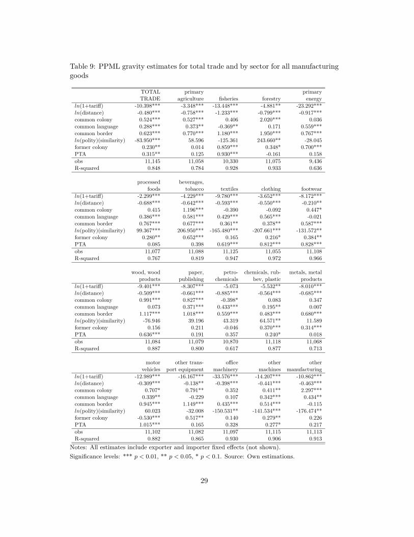
Table 9: PPML gravity estimates for total trade and by sector for all manufacturinggoods

TOTAL primary primaryTRADE agriculture fisheries forestry energy

𝑙𝑛(1+tariff) -10.398*** -3.348*** -13.448*** -4.881** -23.292***𝑙𝑛(distance) -0.480*** -0.758*** -1.233*** -0.799*** -0.917***common colony 0.524*** 0.527*** 0.406 2.020*** 0.036common language 0.288*** 0.373** -0.369** 0.171 0.559***common border 0.623*** 0.770*** 1.180*** 1.950*** 0.767***𝑙𝑛(polity)(similarity) -83.950*** 58.596 -125.361 243.660** -28.045former colony 0.230** 0.014 0.859*** 0.348* 0.700***PTA 0.315** 0.125 0.930*** -0.161 0.158obs 11,145 11,058 10,330 11,075 9,436R-squared 0.848 0.784 0.928 0.933 0.636

processed beverages,foods tobacco textiles clothing footwear

𝑙𝑛(1+tariff) -2.299*** -4.229*** -9.780*** -3.652*** -8.172***𝑙𝑛(distance) -0.688*** -0.642*** -0.593*** -0.550*** -0.210**common colony 0.415 1.196*** -0.390 -0.092 0.447*common language 0.386*** 0.581*** 0.429*** 0.565*** -0.021common border 0.767*** 0.677*** 0.361** 0.378** 0.587***𝑙𝑛(polity)(similarity) 99.367*** 206.950*** -165.480*** -207.661*** -131.572**former colony 0.280** 0.652*** 0.165 0.216* 0.384**PTA 0.085 0.398 0.619*** 0.812*** 0.828***obs 11,077 11,088 11,125 11,055 11,108R-squared 0.767 0.819 0.947 0.972 0.966

wood, wood paper, petro- chemicals, rub- metals, metalproducts publishing chemicals bev, plastic products

𝑙𝑛(1+tariff) -9.401*** -8.307*** -5.073 -5.532** -8.010***𝑙𝑛(distance) -0.509*** -0.661*** -0.885*** -0.564*** -0.685***common colony 0.991*** 0.827*** -0.398* 0.083 0.347common language 0.073 0.371*** 0.433*** 0.195** 0.007common border 1.117*** 1.018*** 0.559*** 0.483*** 0.680***𝑙𝑛(polity)(similarity) -76.946 39.196 43.319 64.571** 11.589former colony 0.156 0.211 -0.046 0.370*** 0.314***PTA 0.636*** 0.191 0.357 0.240* 0.018obs 11,084 11,079 10,870 11,118 11,068R-squared 0.887 0.800 0.617 0.877 0.713

motor other trans- office other othervehicles port equipment machinery machines manufacturing

𝑙𝑛(1+tariff) -12.989*** -16.167*** -33.576*** -14.207*** -10.862***𝑙𝑛(distance) -0.309*** -0.138** -0.398*** -0.441*** -0.463***common colony 0.707* 0.791** 0.352 0.411** 2.297***common language 0.339** -0.229 0.107 0.342*** 0.434**common border 0.945*** 1.149*** 0.435*** 0.514*** -0.115𝑙𝑛(polity)(similarity) 60.023 -32.008 -150.531** -141.534*** -176.474**former colony -0.530*** 0.517** 0.140 0.279** 0.226PTA 1.015*** 0.165 0.328 0.277* 0.217obs 11,102 11,082 11,097 11,115 11,113R-squared 0.882 0.865 0.930 0.906 0.913

Notes: All estimates include exporter and importer fixed effects (not shown).Significance levels: *** 𝑝 < 0.01, ** 𝑝 < 0.05, * 𝑝 < 0.1. Source: Own estimations.

29

B CGE model summaryThe CGE modeling frameworks allow for economy-wide economic analysis. By em-ploying a balanced and internally consistent global database, in tandem with aneconomic model that describes economic activity for a variety of sectors and agentsin the global economy, any change in exogenous variables can be assessed to under-stand the effects on endogenous variables in the model. The key features of a CGEframework include the model that describes economic activity and behavior, the un-derlying database that accounts for initial equilibrium of the global economy, as wellas the suit of parameters that drive responses of agents to any given perturbationto the initial equilibrium.

B.1 Standard GTAP model

The particular model we use in this paper is a modified version of the standardGTAP-class CGE model. The main characteristics and references to the standardGTAP model can be found at: www.gtap.agecon.purdue.edu/models/current.asp,while Hertel (2013) and Rutherford and Paltsev (2000) provide a detailed discussionof the GTAP-class models. Here we provide a summary of this model.

The standard GTAP model describes the global economy as a whole and theinteraction among economic agents. Macroeconomic factors are accounted for, in-cluding GDP, savings and investment, as well as wages and rents. Microeconomicfactors are also described including supply-side factors, firms’ production decisions;demand-side factors, including behavior by households and governments; factor mar-ket conditions governing labor and capital, as well as international trade. The modelis employed in tandem with actual data from a given base year to quantify the ef-fects of an economic shock that causes a movement from the initial equilibrium of theeconomy (see Narayanan et al. (2012) for documentation on the GTAP 8 database,and Hertel (2013) on the full database project). The initial condition of the modelis that supply and demand are in balance at some equilibrium set of prices andquantities where workers are satisfied with their wages and employment, consumersare satisfied with their basket of goods, producers are satisfied with their input andoutput quantities and savings are fully expended on investments. Adjustment to anew equilibrium, governed by behavioral equations and parameters in the model,are largely driven by price linkage equations that link all economic activity in themarket. For any perturbation to the initial equilibrium, all endogenous variables(i.e. prices and quantities) adjust simultaneously until the economy reaches a newequilibrium. Constraints on the adjustment to a new equilibrium include a suit ofaccounting relationships that dictate that in aggregate, the supply of goods equalsthe demand for goods, total exports equals total imports, all (available) workersand capital stock is employed, and global savings equals global investment; unlessadjustments to these assumptions are modified for a particular application. Eco-nomic behavior drives the adjustment of quantities and prices given that consumersmaximize utility given the price of goods and consumers’ budget constraints, and

30

producers minimize costs, given input prices, the level of output and productiontechnology.

From the consumption side, the model includes a Constant Difference of Elas-ticities (CDE) specification for household demand. Private consumption demandsfor composite commodities are modeled on a per capita basis, and each region isrepresented by a regional household. All partial elasticities of substitution for com-posite commodities as well as price and income elasticities drive demand responsesto economic shocks.

The standard GTAP model provides an explicit and detailed treatment of inter-national trade and transport margins. Bilateral trade is handled via CES (constantelasticity of substitution) preferences for intermediate and final goods, using theso-called Armington assumption, where the substitution of domestics and imports–as well as product differentiation– is driven by the region of origin (i.e. by importsource). This assumption is generic to most CGE models as it is a simple deviceto account for "cross-hauling" of trade (i.e. the empirical observation that countriesoften simultaneously import and export goods in the same product category).

B.2 Particular CGE model specification of the paper

In our model, however, we employ a modified version of the standard GTAP modelthat allows for monopolistic competition and increasing returns to scale (Krugman,1980; Francois et al., 2013a).31 In this specification there is a representative firmfor each sector that produces a unique variety of the good and hence, behaves as amonopolist in their specific market.

This specification substitutes the commonly used Armington specification forimport demands, by allowing the demand for differentiated intermediate productsto be based on firms, or product variety, rather than over regions of origin. Whilefirms behave as monopolists, the existence of free entry drives economic profits tozero, so that pricing is at average cost, as is the case in the standard GTAP modelspecification.

In particular, we use the love-of-variety –i.e. Spence-Dixit-Stiglitz (SDS)– pref-erences for intermediate and final goods for non-agricultural sectors. Within a rep-resentative firm, one can assume individual varieties are symmetrical in terms ofselling at the same price and quantity, but that increases in the number of varietiesyielding benefits because they are perceived to be different by intermediate and finaldemand agents. This approach can be nested within a basic CES demand systemthat includes both Armington- and SDS-type demand systems for individual sectorsusing Ethier and Krugman-type monopolistic competition models –i.e. differentiatedintermediate and differentiated consumer goods.32

31 Moreover, this theoretical specification of the trade structure based on Krugman (1980), canbe directly linked to a corresponding gravity equation (Costinot and Rodríguez-Clare, 2013).

32This can be done because one can reduce Ethier-Krugman-models algebraically to Armington-type demand systems with external scale economies linked to a variety of effects (Francois andRoland-Holst, 1997; Francois and Nelson, 2002).

31

Economies of scale are then modeled using the concept of variety-scaled goods.We can define ’variety-scaled output’, which refers to physical quantities, with a’scaling’ or quality coefficient that reflects the varieties embodied on total physicaloutput. This variety-scaled output can be substituted directly into an Armington-type demand system. The precise modeling in the CGE-GTAP code is done bymeans of a closure swap that yields output level and variety scaling effects at thesectoral level. This implies that sectoral productivity is now endogenous in themodel and it adjusts to capture the output scale and variety effects.

Another key specification that is distinguishes our model is the calculation ofchanges in 𝐶𝑂2 emissions by region and sector, given the emergence of new traderoutes. The inclusion of 𝐶𝑂2 data and the corresponding model-predicted changesin 𝐶𝑂2 emissions allow for the analysis of environmental impacts that are expected,given the future use of the NSR.

B.3 CGE model limitations and alternative model specifications

One of the limitations of CGE models is that it assumes that after an exogenousshock (e.g. a trade cost change) the economy adjusts instantly. In practice, theseadjustments may take time and the costs linked to these changes (for instance,shifting production and workers between sectors, changing consumption patterns,adjusting tax revenues between different sources) may be significant and CGE modelsare not designed to assess these adjustment costs. Nevertheless, the magnitude ofthe required changes implicit in the model simulations can provide a guide intoassessing these short-term costs. However, in the context of this paper, where theuse of the NSR and NWR is expected to be a gradual and medium to long-termprocess, the required adjustments will be spread over time and thus, more easilyabsorbed by different regions within several years.

More recently, a series of papers analyze the welfare and overall macroeconomicoutcomes of employing different market structures and trade specifications into quan-titative trade models (cf. Costinot and Rodríguez-Clare, 2013). These micro-theorybased econometric models are highly stylized quantification methods, that are wellgrounded in recent micro-economic theory, and provide clear theoretical links be-tween market structure and the gravity equation. However, given that most of thesemodels are single-sector specifications, their scope is very limited in terms of actualanalysis, and they are not capable of dealing with detailed analysis of global tradeissues. In particular, these models are not able to deal with intermediate linkagesassociated with global supply chains and their associated carbon emissions; on howemissions are linked to country- and sector-specific transport activities; and on howto separate actual transport costs from time related costs that are sector-specificin nature. These are issues central to the evaluation of the economic and environ-mental effects of the Arctic routes that can only be tackled using a CGE model.The exception is a sub-class of models that employ a multi-sector trade structurespecification following Eaton and Kortum (2002). However, these type of modelsare still not detailed enough to assess the effects of trade changes associated with

32

alternative shipping routes as the NSR and NWR. In particular, they do not havean explicit international transport section, which is the key variable that explainsthe linkage between shipping trade cost reductions that are directly associated withthe Arctic shipping lanes.

Different market structure specifications may generate different sectoral out-comes depending on the particulars of the specific sectors and how they are modeled–see Francois et al. (2013a) for a more technical discussion of demand systems anddifferent market structures. However, at the aggregate level, there will be relativelysmall differences between model specifications. For example, Arkolakis et al. (2012)point out that welfare effects are similar for the different trade structure specifica-tions.

Since the main driving force in our bilateral trade results is a reduction on thetrading distance between partners that follows from the gravity model of trade, itis expected that similar bilateral trade results and overall welfare and macroeco-nomic effects will be found using a wider set of trade models –although the outputimplications can be different between both sets of models for specific sectors.

33

C Additional tables and figures

Table 10: Different distance values for selected countries

From: To: Great-circleformula (km)

SSR (km) NSR (km) NSR againstSSR % change

China Netherlands 7,831 19,942 15,436 -23%China Belgium 7,971 19,914 15,477 -22%China Germany 7,363 20,478 15,942 -22%China United Kingdom 8,151 19,799 14,898 -25%

Japan Netherlands 9,303 20,996 13,172 -37%Japan Belgium 9,464 20,976 13,345 -36%Japan Germany 8,928 21,536 13,083 -39%Japan United Kingdom 9,574 20,779 13,182 -37%

South Korea Netherlands 8,573 20,479 14,200 -31%South Korea Belgium 8,722 20,458 14,373 -30%South Korea Germany 8,140 21,019 14,110 -33%South Korea United Kingdom 8,875 20,262 14,210 -30%

Taiwan Netherlands 9,457 18,822 15,601 -17%Taiwan Belgium 9,587 18,801 15,774 -16%Taiwan Germany 8,959 19,362 15,511 -20%Taiwan United Kingdom 9,790 18,605 15,611 -16%

Sources: Great-circle distances taken from the GeoDist database from CEPII. SSR and NSRdistances are own estimations based on data from AtoBviaC, BLM Shipping, and Liu and Kronbak(2010).

34

Table 11: Sectoral description and aggregation

Code Sector description Aggregated GTAP sectors

S01 Agricultural products OSD (oil seeds), C_B (sugar cane), PFB (plant-based fibbers), CTL(cattle), OAP (animal prods nec), RMK (raw milk), WOL (wool)

S02 Motor vehicles MVH (motor vehicles and parts)S03 Beverages and tobacco B_T (beverages & tobacco products)S04 Chemicals CRP (Chemical, rubber and plastic products)S05 Clothing WAP (wearing apparel)S06 Plant products OCR (crops nec)S07 Fisheries FSH (fishing)S08 Processed foods PDR (paddy rice), WHT (wheat), GRO (cereal grains nec), V_F (veg-

etables & fruits), CMT (bovine meat prods), OMT (Meat prods nec),VOL (vegetable oils), MIL (diary prod), PCR (processed rice), SGR(sugar), OFD (food products nec)

S09 Leather products LEA (leather products)S10 Forestry FRS (forestry)S11 Metals I_S (ferrous metals), NFM (metals nec), FMP (metal products)S12 Office machinery ELE (electronic equipment)S13 Other machinery OME (machinery and equipment necS14 Other manufactures NMM (mineral products nec), OMF (manufactures nec)S15 Petrochemicals and gas P_C (Petroleum and coal products), GDT (gas manufacture and distri-

bution)S16 Mining and extraction COA (coal), OIL (oil), GAS (gas), OMN (Minerals nec)S17 Textiles TEX (textiles)S18 Transport equipment OTN (transport equipment nec)S19 Paper products and publishing PPP (paper products and publishing)S20 Wood products LUM (wood products)S21 Transport services OTP (transport nec), WTP (water transport), ATP (air transport)S22 Commercial services WTR (water), CNS (construction), TRD (trade), CMN (communica-

tion), OFI (financial services nec), ISR (insurance), OBS (Business ser-vices nec)

S23 Public and consumer services ELY (electricity), ROS (recreational and other services), OSG (PublicAdministration, Defence, Education, Health), DWE (dwellings)

35

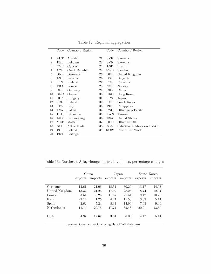
Table 12: Regional aggregation

Code Country / Region Code Country / Region

1 AUT Austria 21 SVK Slovakia2 BEL Belgium 22 SVN Slovenia3 CYP Cyprus 23 ESP Spain4 CZE Czech Republic 24 SWE Sweden5 DNK Denmark 25 GBR United Kingdom6 EST Estonia 26 BGR Bulgaria7 FIN Finland 27 ROU Romania8 FRA France 28 NOR Norway9 DEU Germany 29 CHN China10 GRC Greece 30 HKG Hong Kong11 HUN Hungary 31 JPN Japan12 IRL Ireland 32 KOR South Korea13 ITA Italy 33 PHL Philippines14 LVA Latvia 34 PNG Other Asia Pacific15 LTU Lithuania 35 TWN Taiwan16 LUX Luxembourg 36 USA United States17 MLT Malta 37 OCD Other OECD18 NLD Netherlands 38 SSA Sub-Sahara Africa excl. ZAF19 POL Poland 39 ROW Rest of the World20 PRT Portugal

Table 13: Northeast Asia, changes in trade volumes, percentage changes

China Japan South Koreaexports imports exports imports exports imports

Germany 12.61 21.06 18.51 30.29 13.17 24.03United Kingdom 13.32 21.25 17.92 28.26 8.74 22.94France 3.54 8.25 11.67 21.54 9.42 10.75Italy -2.14 1.25 4.24 11.50 3.09 5.14Spain 2.62 5.24 8.31 14.96 7.65 9.40Netherlands 11.14 20.75 17.74 33.43 20.91 23.30

USA 4.97 12.67 3.34 6.06 4.47 5.14

Source: Own estimations using the GTAP database.

36

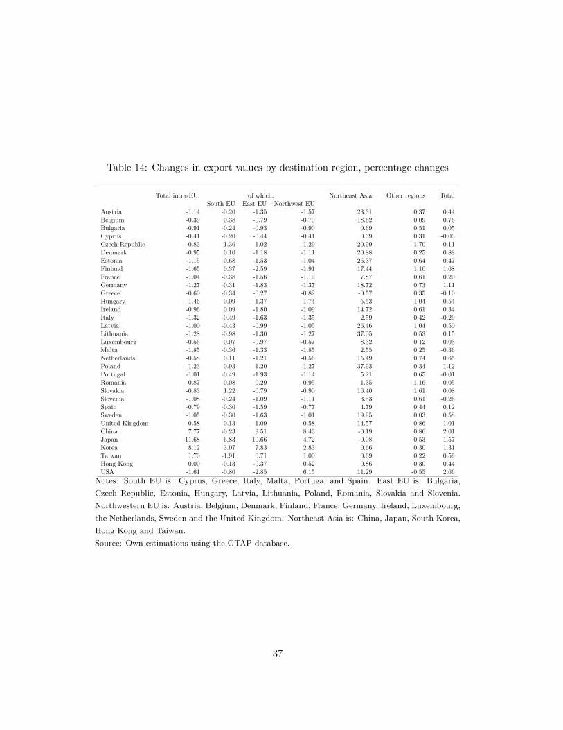
Table 14: Changes in export values by destination region, percentage changes

Total intra-EU, of which: Northeast Asia Other regions TotalSouth EU East EU Northwest EU

Austria -1.14 -0.20 -1.35 -1.57 23.31 0.37 0.44Belgium -0.39 0.38 -0.79 -0.70 18.62 0.09 0.76Bulgaria -0.91 -0.24 -0.93 -0.90 0.69 0.51 0.05Cyprus -0.41 -0.20 -0.44 -0.41 0.39 0.31 -0.03Czech Republic -0.83 1.36 -1.02 -1.29 20.99 1.70 0.11Denmark -0.95 0.10 -1.18 -1.11 20.88 0.25 0.88Estonia -1.15 -0.68 -1.53 -1.04 26.37 0.64 0.47Finland -1.65 0.37 -2.59 -1.91 17.44 1.10 1.68France -1.04 -0.38 -1.56 -1.19 7.87 0.61 0.20Germany -1.27 -0.31 -1.83 -1.37 18.72 0.73 1.11Greece -0.60 -0.34 -0.27 -0.82 -0.57 0.35 -0.10Hungary -1.46 0.09 -1.37 -1.74 5.53 1.04 -0.54Ireland -0.96 0.09 -1.80 -1.09 14.72 0.61 0.34Italy -1.32 -0.49 -1.63 -1.35 2.59 0.42 -0.29Latvia -1.00 -0.43 -0.99 -1.05 26.46 1.04 0.50Lithuania -1.28 -0.98 -1.30 -1.27 37.05 0.53 0.15Luxembourg -0.56 0.07 -0.97 -0.57 8.32 0.12 0.03Malta -1.85 -0.36 -1.33 -1.85 2.55 0.25 -0.36Netherlands -0.58 0.11 -1.21 -0.56 15.49 0.74 0.65Poland -1.23 0.93 -1.20 -1.27 37.93 0.34 1.12Portugal -1.01 -0.49 -1.93 -1.14 5.21 0.65 -0.01Romania -0.87 -0.08 -0.29 -0.95 -1.35 1.16 -0.05Slovakia -0.83 1.22 -0.79 -0.90 16.40 1.61 0.08Slovenia -1.08 -0.24 -1.09 -1.11 3.53 0.61 -0.26Spain -0.79 -0.30 -1.59 -0.77 4.79 0.44 0.12Sweden -1.05 -0.30 -1.63 -1.01 19.95 0.03 0.58United Kingdom -0.58 0.13 -1.09 -0.58 14.57 0.86 1.01China 7.77 -0.23 9.51 8.43 -0.19 0.86 2.01Japan 11.68 6.83 10.66 4.72 -0.08 0.53 1.57Korea 8.12 3.07 7.83 2.83 0.66 0.30 1.31Taiwan 1.70 -1.91 0.71 1.00 0.69 0.22 0.59Hong Kong 0.00 -0.13 -0.37 0.52 0.86 0.30 0.44USA -1.61 -0.80 -2.85 6.15 11.29 -0.55 2.66

Notes: South EU is: Cyprus, Greece, Italy, Malta, Portugal and Spain. East EU is: Bulgaria,Czech Republic, Estonia, Hungary, Latvia, Lithuania, Poland, Romania, Slovakia and Slovenia.Northwestern EU is: Austria, Belgium, Denmark, Finland, France, Germany, Ireland, Luxembourg,the Netherlands, Sweden and the United Kingdom. Northeast Asia is: China, Japan, South Korea,Hong Kong and Taiwan.Source: Own estimations using the GTAP database.

37

Table 15: Sectoral changes in export sales to USA for selected countries, percentagechanges

FRA DEU ITA NLD ESP GBR CHN JPN KORSector:S01 2.4 2.2 2.5 1.5 2.3 2.1 6.9 14.6 12.1S02 0.3 -0.9 -0.4 0.9 0.1 0.3 7.7 2.6 1.7S03 0.0 0.3 -0.2 0.2 0.0 0.2 7.5 9.9 9.9S04 -0.4 0.6 -0.4 -0.5 -0.4 0.3 6.7 7.0 5.2S05 -0.8 -1.0 -0.8 -1.6 -0.5 -1.8 5.5 5.3 5.2S06 0.6 0.5 0.8 0.2 0.6 0.5 5.7 11.9 8.8S07 -1.2 4.0 0.4 2.3 0.1 2.8 0.0 14.0 7.4S08 0.2 0.5 0.0 0.5 0.2 0.5 6.4 10.2 9.4S09 -1.3 0.0 -1.7 1.8 -1.3 0.3 1.0 5.7 2.5S10 -0.2 -10.6 0.5 -2.4 2.0 3.8 4.9 15.5 11.7S11 0.0 -1.4 0.2 -1.5 -0.3 -0.3 6.4 7.9 7.7S12 -1.5 0.7 -3.2 3.8 -1.0 3.4 2.0 1.7 0.1S13 -0.8 -0.3 -1.2 -0.1 -0.8 0.2 4.8 2.8 4.5S14 -2.9 -1.1 -4.4 2.8 -3.7 0.2 3.5 0.0 6.9S15 0.1 0.6 0.2 0.5 0.2 0.2 7.8 9.2 8.0S16 2.8 0.4 3.6 4.0 0.8 2.6 23.9 21.4 48.3S17 -1.4 -0.2 -2.4 1.0 -1.8 0.4 2.8 4.7 4.3S18 0.0 -0.2 -0.8 0.8 -0.4 0.1 8.9 1.0 1.5S19 -0.4 -0.4 -0.6 -0.2 -0.6 0.2 8.0 8.5 9.0S20 -1.1 0.0 -0.8 2.0 -0.8 5.5 7.6 5.9 6.6S21 0.1 0.4 0.0 0.3 0.2 0.2 0.6 -0.2 0.0S22 -0.1 0.1 -0.4 0.1 0.0 0.1 0.6 -0.5 0.1S23 1.3 0.1 1.2 -0.2 1.2 0.9 -2.3 -1.1 -1.7

Simple average -0.2 -0.2 -0.3 0.7 -0.2 1.0 5.5 6.9 7.4

Notes: The description of each sector is given in Table 11.Source: Own estimations using the GTAP database.

38

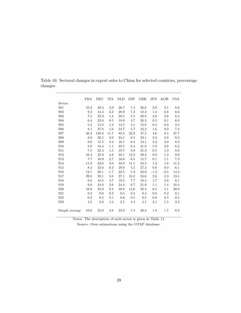
Table 16: Sectoral changes in export sales to China for selected countries, percentagechanges

FRA DEU ITA NLD ESP GBR JPN KOR USASector:S01 10.2 30.4 2.9 26.7 7.4 26.6 3.9 3.1 8.6S02 9.2 14.4 3.2 20.9 7.3 12.3 1.3 0.8 6.6S03 7.5 22.9 1.4 20.5 5.5 20.8 2.0 2.6 8.4S04 6.4 23.0 0.5 18.9 4.7 20.3 0.5 0.1 6.0S05 5.2 15.8 1.2 13.5 4.1 12.8 0.4 0.9 3.4S06 8.1 27.8 1.0 24.7 5.7 24.2 1.6 0.0 7.3S07 46.3 128.6 11.7 85.5 22.9 47.5 4.6 6.5 37.7S08 8.9 26.5 2.0 24.1 6.5 23.1 2.3 2.8 9.3S09 9.0 15.5 4.4 16.1 6.4 13.1 3.2 4.0 8.3S10 8.8 16.4 1.1 23.5 8.4 31.0 5.9 3.6 6.2S11 7.5 22.4 1.5 19.7 5.0 21.3 0.5 1.3 8.0S12 10.4 25.9 4.8 32.1 12.3 29.3 0.0 1.3 9.9S13 7.7 16.9 2.7 16.6 6.5 15.7 0.1 1.1 7.3S14 11.9 33.0 3.0 33.8 11.1 24.5 1.3 1.6 11.2S15 8.2 32.6 0.3 29.0 5.5 27.3 0.0 0.0 6.1S16 12.1 20.1 -1.7 23.5 5.3 22.9 -1.2 -3.5 14.3S17 29.0 28.1 5.0 27.1 10.2 24.6 2.6 2.3 13.5S18 6.8 10.5 4.7 19.5 7.7 10.4 1.7 2.6 6.1S19 9.0 24.0 2.6 24.4 6.7 21.9 1.1 1.4 10.4S20 16.8 35.0 8.2 38.8 14.6 32.4 6.5 5.1 20.0S21 0.3 0.6 0.2 0.5 0.4 0.4 0.0 0.2 0.1S22 0.3 0.5 0.1 0.6 0.5 0.5 0.0 0.5 0.5S23 4.5 3.3 4.4 3.1 4.4 4.1 2.1 1.5 3.3

Simple average 10.6 25.0 2.8 23.6 7.3 20.3 1.8 1.7 9.2

Notes: The description of each sector is given in Table 11.Source: Own estimations using the GTAP database.

39

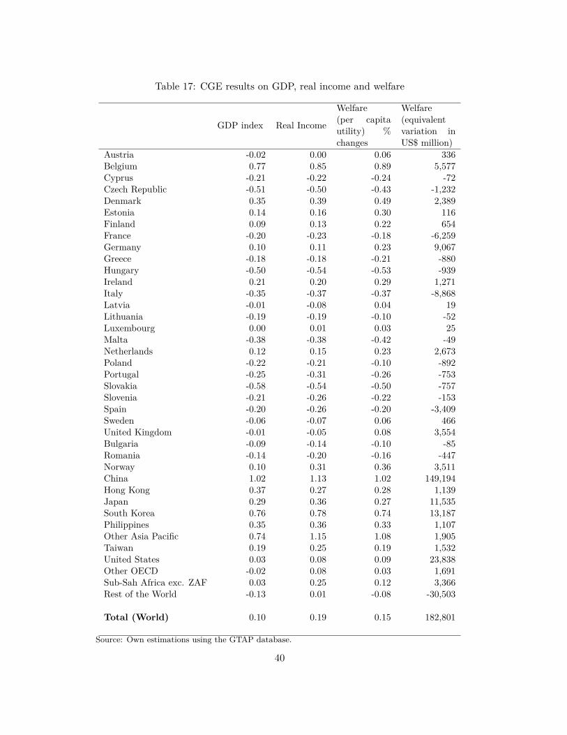
Table 17: CGE results on GDP, real income and welfare

GDP index Real Income

Welfare(per capitautility) %changes

Welfare(equivalentvariation inUS$ million)

Austria -0.02 0.00 0.06 336Belgium 0.77 0.85 0.89 5,577Cyprus -0.21 -0.22 -0.24 -72Czech Republic -0.51 -0.50 -0.43 -1,232Denmark 0.35 0.39 0.49 2,389Estonia 0.14 0.16 0.30 116Finland 0.09 0.13 0.22 654France -0.20 -0.23 -0.18 -6,259Germany 0.10 0.11 0.23 9,067Greece -0.18 -0.18 -0.21 -880Hungary -0.50 -0.54 -0.53 -939Ireland 0.21 0.20 0.29 1,271Italy -0.35 -0.37 -0.37 -8,868Latvia -0.01 -0.08 0.04 19Lithuania -0.19 -0.19 -0.10 -52Luxembourg 0.00 0.01 0.03 25Malta -0.38 -0.38 -0.42 -49Netherlands 0.12 0.15 0.23 2,673Poland -0.22 -0.21 -0.10 -892Portugal -0.25 -0.31 -0.26 -753Slovakia -0.58 -0.54 -0.50 -757Slovenia -0.21 -0.26 -0.22 -153Spain -0.20 -0.26 -0.20 -3,409Sweden -0.06 -0.07 0.06 466United Kingdom -0.01 -0.05 0.08 3,554Bulgaria -0.09 -0.14 -0.10 -85Romania -0.14 -0.20 -0.16 -447Norway 0.10 0.31 0.36 3,511China 1.02 1.13 1.02 149,194Hong Kong 0.37 0.27 0.28 1,139Japan 0.29 0.36 0.27 11,535South Korea 0.76 0.78 0.74 13,187Philippines 0.35 0.36 0.33 1,107Other Asia Pacific 0.74 1.15 1.08 1,905Taiwan 0.19 0.25 0.19 1,532United States 0.03 0.08 0.09 23,838Other OECD -0.02 0.08 0.03 1,691Sub-Sah Africa exc. ZAF 0.03 0.25 0.12 3,366Rest of the World -0.13 0.01 -0.08 -30,503

Total (World) 0.10 0.19 0.15 182,801

Source: Own estimations using the GTAP database.

40

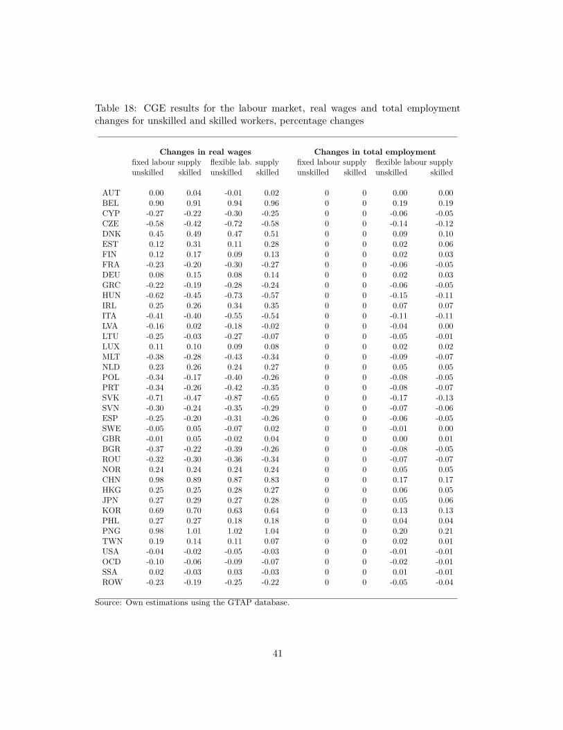
Table 18: CGE results for the labour market, real wages and total employmentchanges for unskilled and skilled workers, percentage changes

Changes in real wages Changes in total employmentfixed labour supply flexible lab. supply fixed labour supply flexible labour supplyunskilled skilled unskilled skilled unskilled skilled unskilled skilled

AUT 0.00 0.04 -0.01 0.02 0 0 0.00 0.00BEL 0.90 0.91 0.94 0.96 0 0 0.19 0.19CYP -0.27 -0.22 -0.30 -0.25 0 0 -0.06 -0.05CZE -0.58 -0.42 -0.72 -0.58 0 0 -0.14 -0.12DNK 0.45 0.49 0.47 0.51 0 0 0.09 0.10EST 0.12 0.31 0.11 0.28 0 0 0.02 0.06FIN 0.12 0.17 0.09 0.13 0 0 0.02 0.03FRA -0.23 -0.20 -0.30 -0.27 0 0 -0.06 -0.05DEU 0.08 0.15 0.08 0.14 0 0 0.02 0.03GRC -0.22 -0.19 -0.28 -0.24 0 0 -0.06 -0.05HUN -0.62 -0.45 -0.73 -0.57 0 0 -0.15 -0.11IRL 0.25 0.26 0.34 0.35 0 0 0.07 0.07ITA -0.41 -0.40 -0.55 -0.54 0 0 -0.11 -0.11LVA -0.16 0.02 -0.18 -0.02 0 0 -0.04 0.00LTU -0.25 -0.03 -0.27 -0.07 0 0 -0.05 -0.01LUX 0.11 0.10 0.09 0.08 0 0 0.02 0.02MLT -0.38 -0.28 -0.43 -0.34 0 0 -0.09 -0.07NLD 0.23 0.26 0.24 0.27 0 0 0.05 0.05POL -0.34 -0.17 -0.40 -0.26 0 0 -0.08 -0.05PRT -0.34 -0.26 -0.42 -0.35 0 0 -0.08 -0.07SVK -0.71 -0.47 -0.87 -0.65 0 0 -0.17 -0.13SVN -0.30 -0.24 -0.35 -0.29 0 0 -0.07 -0.06ESP -0.25 -0.20 -0.31 -0.26 0 0 -0.06 -0.05SWE -0.05 0.05 -0.07 0.02 0 0 -0.01 0.00GBR -0.01 0.05 -0.02 0.04 0 0 0.00 0.01BGR -0.37 -0.22 -0.39 -0.26 0 0 -0.08 -0.05ROU -0.32 -0.30 -0.36 -0.34 0 0 -0.07 -0.07NOR 0.24 0.24 0.24 0.24 0 0 0.05 0.05CHN 0.98 0.89 0.87 0.83 0 0 0.17 0.17HKG 0.25 0.25 0.28 0.27 0 0 0.06 0.05JPN 0.27 0.29 0.27 0.28 0 0 0.05 0.06KOR 0.69 0.70 0.63 0.64 0 0 0.13 0.13PHL 0.27 0.27 0.18 0.18 0 0 0.04 0.04PNG 0.98 1.01 1.02 1.04 0 0 0.20 0.21TWN 0.19 0.14 0.11 0.07 0 0 0.02 0.01USA -0.04 -0.02 -0.05 -0.03 0 0 -0.01 -0.01OCD -0.10 -0.06 -0.09 -0.07 0 0 -0.02 -0.01SSA 0.02 -0.03 0.03 -0.03 0 0 0.01 -0.01ROW -0.23 -0.19 -0.25 -0.22 0 0 -0.05 -0.04

Source: Own estimations using the GTAP database.

41

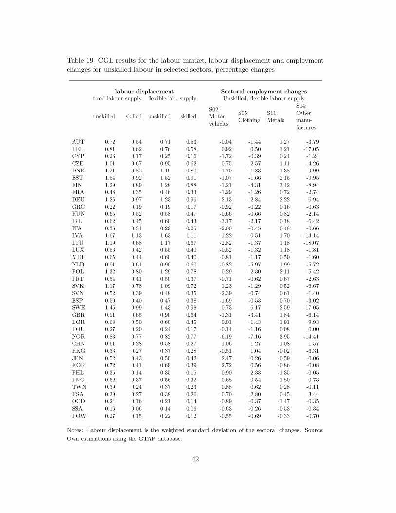
Table 19: CGE results for the labour market, labour displacement and employmentchanges for unskilled labour in selected sectors, percentage changes

labour displacement Sectoral employment changesfixed labour supply flexible lab. supply Unskilled, flexible labour supply

unskilled skilled unskilled skilledS02:Motorvehicles

S05:Clothing

S11:Metals

S14:Othermanu-factures

AUT 0.72 0.54 0.71 0.53 -0.04 -1.44 1.27 -3.79BEL 0.81 0.62 0.76 0.58 0.92 0.50 1.21 -17.05CYP 0.26 0.17 0.25 0.16 -1.72 -0.39 0.24 -1.24CZE 1.01 0.67 0.95 0.62 -0.75 -2.57 1.11 -4.26DNK 1.21 0.82 1.19 0.80 -1.70 -1.83 1.38 -9.99EST 1.54 0.92 1.52 0.91 -1.07 -1.66 2.15 -9.95FIN 1.29 0.89 1.28 0.88 -1.21 -4.31 3.42 -8.94FRA 0.48 0.35 0.46 0.33 -1.29 -1.26 0.72 -2.74DEU 1.25 0.97 1.23 0.96 -2.13 -2.84 2.22 -6.94GRC 0.22 0.19 0.19 0.17 -0.92 -0.22 0.16 -0.63HUN 0.65 0.52 0.58 0.47 -0.66 -0.66 0.82 -2.14IRL 0.62 0.45 0.60 0.43 -3.17 -2.17 0.18 -6.42ITA 0.36 0.31 0.29 0.25 -2.00 -0.45 0.48 -0.66LVA 1.67 1.13 1.63 1.11 -1.22 -0.51 1.70 -14.14LTU 1.19 0.68 1.17 0.67 -2.82 -1.37 1.18 -18.07LUX 0.56 0.42 0.55 0.40 -0.52 -1.32 1.18 -1.81MLT 0.65 0.44 0.60 0.40 -0.81 -1.17 0.50 -1.60NLD 0.91 0.61 0.90 0.60 -0.82 -5.97 1.99 -5.72POL 1.32 0.80 1.29 0.78 -0.29 -2.30 2.11 -5.42PRT 0.54 0.41 0.50 0.37 -0.71 -0.62 0.67 -2.63SVK 1.17 0.78 1.09 0.72 1.23 -1.29 0.52 -6.67SVN 0.52 0.39 0.48 0.35 -2.39 -0.74 0.61 -1.40ESP 0.50 0.40 0.47 0.38 -1.69 -0.53 0.70 -3.02SWE 1.45 0.99 1.43 0.98 -0.73 -6.17 2.59 -17.05GBR 0.91 0.65 0.90 0.64 -1.31 -3.41 1.84 -6.14BGR 0.68 0.50 0.60 0.45 -0.01 -1.43 -1.91 -9.93ROU 0.27 0.20 0.24 0.17 -0.14 -1.16 0.08 0.00NOR 0.83 0.77 0.82 0.77 -6.19 -7.16 3.95 -14.41CHN 0.61 0.28 0.58 0.27 1.06 1.27 -1.08 1.57HKG 0.36 0.27 0.37 0.28 -0.51 1.04 -0.02 -6.31JPN 0.52 0.43 0.50 0.42 2.47 -0.26 -0.59 -0.06KOR 0.72 0.41 0.69 0.39 2.72 0.56 -0.86 -0.08PHL 0.35 0.14 0.35 0.15 0.90 2.33 -1.35 -0.05PNG 0.62 0.37 0.56 0.32 0.68 0.54 1.80 0.73TWN 0.39 0.24 0.37 0.23 0.88 0.62 0.28 -0.11USA 0.39 0.27 0.38 0.26 -0.70 -2.80 0.45 -3.44OCD 0.24 0.16 0.21 0.14 -0.89 -0.37 -1.47 -0.35SSA 0.16 0.06 0.14 0.06 -0.63 -0.26 -0.53 -0.34ROW 0.27 0.15 0.22 0.12 -0.55 -0.69 -0.33 -0.70

Notes: Labour displacement is the weighted standard deviation of the sectoral changes. Source:Own estimations using the GTAP database.

42

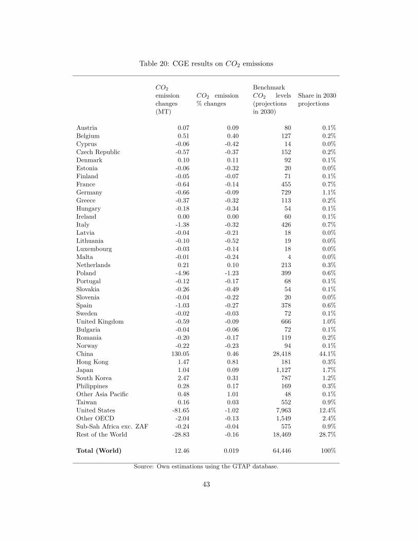
Table 20: CGE results on 𝐶𝑂2 emissions

𝐶𝑂2emissionchanges(MT)

𝐶𝑂2 emission% changes

Benchmark𝐶𝑂2 levels(projectionsin 2030)

Share in 2030projections

Austria 0.07 0.09 80 0.1%Belgium 0.51 0.40 127 0.2%Cyprus -0.06 -0.42 14 0.0%Czech Republic -0.57 -0.37 152 0.2%Denmark 0.10 0.11 92 0.1%Estonia -0.06 -0.32 20 0.0%Finland -0.05 -0.07 71 0.1%France -0.64 -0.14 455 0.7%Germany -0.66 -0.09 729 1.1%Greece -0.37 -0.32 113 0.2%Hungary -0.18 -0.34 54 0.1%Ireland 0.00 0.00 60 0.1%Italy -1.38 -0.32 426 0.7%Latvia -0.04 -0.21 18 0.0%Lithuania -0.10 -0.52 19 0.0%Luxembourg -0.03 -0.14 18 0.0%Malta -0.01 -0.24 4 0.0%Netherlands 0.21 0.10 213 0.3%Poland -4.96 -1.23 399 0.6%Portugal -0.12 -0.17 68 0.1%Slovakia -0.26 -0.49 54 0.1%Slovenia -0.04 -0.22 20 0.0%Spain -1.03 -0.27 378 0.6%Sweden -0.02 -0.03 72 0.1%United Kingdom -0.59 -0.09 666 1.0%Bulgaria -0.04 -0.06 72 0.1%Romania -0.20 -0.17 119 0.2%Norway -0.22 -0.23 94 0.1%China 130.05 0.46 28,418 44.1%Hong Kong 1.47 0.81 181 0.3%Japan 1.04 0.09 1,127 1.7%South Korea 2.47 0.31 787 1.2%Philippines 0.28 0.17 169 0.3%Other Asia Pacific 0.48 1.01 48 0.1%Taiwan 0.16 0.03 552 0.9%United States -81.65 -1.02 7,963 12.4%Other OECD -2.04 -0.13 1,549 2.4%Sub-Sah Africa exc. ZAF -0.24 -0.04 575 0.9%Rest of the World -28.83 -0.16 18,469 28.7%

Total (World) 12.46 0.019 64,446 100%

Source: Own estimations using the GTAP database.

43

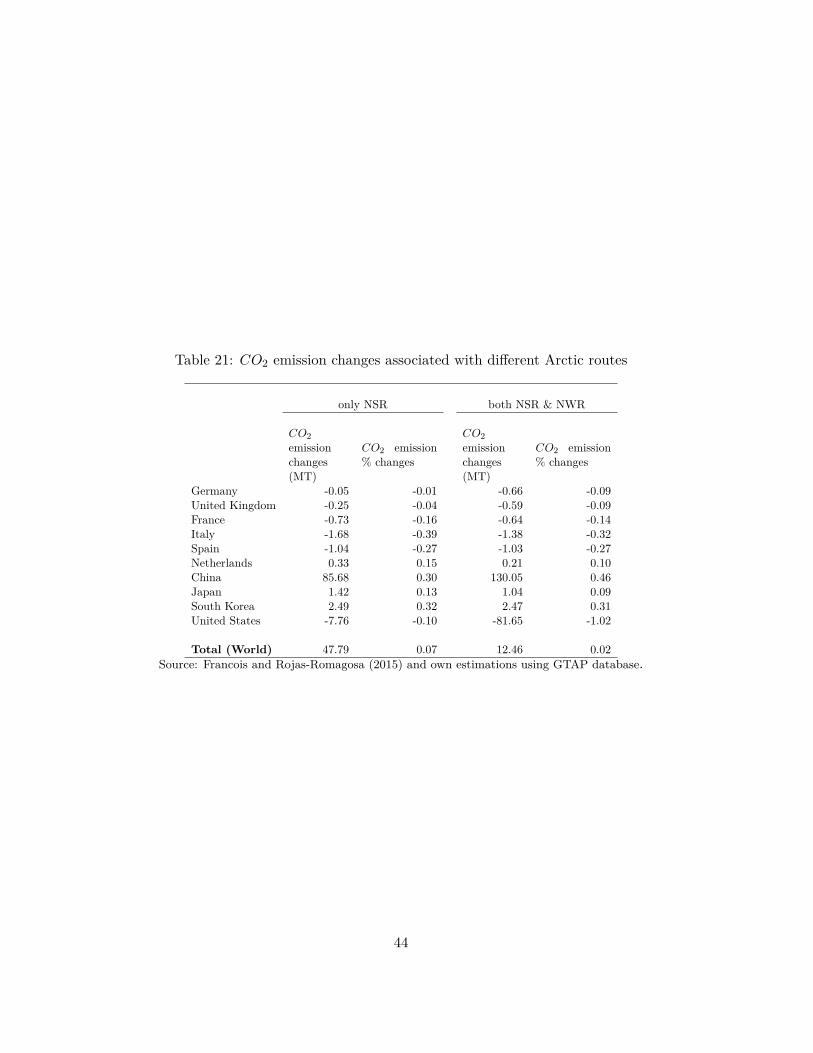
Table 21: 𝐶𝑂2 emission changes associated with different Arctic routes

only NSR both NSR & NWR

𝐶𝑂2emissionchanges(MT)

𝐶𝑂2 emission% changes

𝐶𝑂2emissionchanges(MT)

𝐶𝑂2 emission% changes

Germany -0.05 -0.01 -0.66 -0.09United Kingdom -0.25 -0.04 -0.59 -0.09France -0.73 -0.16 -0.64 -0.14Italy -1.68 -0.39 -1.38 -0.32Spain -1.04 -0.27 -1.03 -0.27Netherlands 0.33 0.15 0.21 0.10China 85.68 0.30 130.05 0.46Japan 1.42 0.13 1.04 0.09South Korea 2.49 0.32 2.47 0.31United States -7.76 -0.10 -81.65 -1.02

Total (World) 47.79 0.07 12.46 0.02Source: Francois and Rojas-Romagosa (2015) and own estimations using GTAP database.

44