TECHNICAL LIBRARY

MEMORANDUM REPORT ARBRL-MR-03126

NUMERICAL DIFFERENTIATION OF NOISY DATA

C. A/lasaitis G. Francis

August 1981

US ARMY ARMAMENT RESEARCH AND DEVELOPMENT COMMAND BALLISTIC RESEARCH LABORATORY ABERDEEN PROVING GROUND, MARYLAND

Approved for public release; distribution unlimited.

Destroy this report when it is no longer needed. Do not return it to the originator.

Secondary distribution of this report by originating or sponsoring activity is prohibited.

Additional copies of this report may be obtained from the National Technical Information Service, U.S. Department of Commerce, Springfield, Virginia 22161.

The findings in this report are not to be construed as an official Department of the Army position, unless so designated by other authorized documents.

Fh^ .(.s-t.' ,'■ t^".i.ia mimtiiS iv ntanufaoturers ' names; in thi^i fevori dcci-: not ,:mc'tLtut,; indoyv.err.ent of arty aormepaial ;:vO(iui:L.

UNCI A.S.ST FT Fn SECURITY CLASSIFICATION OF THIS PAGE (When Data Entered)

REPORT DOCUMENTATION PAGE 1. REPORT NUMBER 2. GOVT ACCESSION NO

MEMORANDUM REPORT ARBRL-MR-03126 4. TITLE (and Subtitle)

NUMERICAL DIFFERENTIATION OF NOISY DATA

7. AUTHORfs;

C. Masaitis G. Francis

9. PERFORMING ORGANIZATION NAME AND ADDRESS

US Army Ballistic Research Laboratory ATTN: DRDAR-BLB Aberdeen Proving Ground, MD 21005 11. CONTROLLING OFFICE NAME AND ADDRESS

US Army Armament Research & Development Command US Army Ballistic Research Laboratory ATTN: DRDAR-BL, APG, MD 21005 14. MONITORING AGENCY NAME ft ADDRESSfi/ dllferent from ControlUng Ollice)

16. DISTRIBUTION ST ATEMEN T fo/(h/s ReporO

READ INSTRUCTIONS BEFORE COMPLETING FORM

3. RECIPIENT'S CATALOG NUMBER

5. TYPE OF REPORT & PERIOD COVERED

Final

6. PERFORMING ORG. REPORT NUMBER

8. CONTRACT OR GRANT NUMBERfs;

10. PROGRAM ELEMENT, PROJECT, TASK AREA a WORK UNIT NUMBERS

RDT8E 1L161102AH43 12. REPORT DATE

AUGUST 1981 13- NUMBER OF PAGES

59 IS. SECURITY CLASS, (ot thia raport;

UNCLASSIFIED ISa. DECLASSIFI CATION/DOWNGRADING

SCHEDULE

Approved for public release; distribution unlimited.

17. DISTRIBUTION STATEMENT (ot the abetract entered In Block 20, It ditferent from Report)

18. SUPPLEMENTARY NOTES

KEY WORDS (Continue on reverae aide It neceaaary and Identify by block number)

Approximation, Numerical Differentiation, Estimation of Derivatives, Smoothing Curve Fitting, Differentiation of Noisy Data. (J^uM^J a^^i^.^^

20. ABSTRACT fContfcua am ravtmm ai<£» tt na<r»aaary and Identity by block number) (hmn)

An algorithm has been developed based on the assumption that a given set of data is representable by a function that is a product of algebraic, trigonom- etric, and exponential polynomials. The degrees of the underlying polynomials, LramStl^f o?tS ^P^^^"9. (optimal multiple of stepsize in tabular data), and the parameters of the approximating function are all selected by the algorithm to minimize an objective function that depends on the variance of the deviation between the data and the fitted function and on the degree of ill-conditioning of

DD/, FORM AM 73 1473 EDrTlON OF t NOV 65 IS OBSOLETE

UNCLASSIFIED SECURITY CLASS!FtCATtOM OF THIS PAGE (Whan Data Entered)

UNCLASSIFIED SECURITY CLASSIFICATION OF THIS PAGEfHTien Date Entetad)

the problem. The algorithm permits choosing global or local fits. Derivatives of any order are obtained either by differentiating the fitted function or by a closed form relation between the model parameters and coefficients of linear combinations that express derivatives in terms of the observed values of the variable. Thus, the algorithm provides local differentiation formulas using parameters derived from global analysis of the data but in terms of the local values of the function. An appendix compares the accuracy of derivatives obtained for synthetic data with the accuracy of other methods.

UNCLASSIFIED SECURITY CLASSIFICATION OF THIS P AGE(When Data Entered)

4.

5.

TABLE OF CONTENTS

Page

INTRODUCTION 5

APPROXIMATION OF TABULAR FUNCTIONS AND THEIR DERIVATIVES 9

2.1 Data Structure 9

2.2 Smoothing and Differentiation 16

DERIVATIVES AS LINEAR COMBINATIONS OF FUNCTIONAL VALUtu -jQ

DERIVATIVES WITH SIMPLE EIGENVALUES 20

ERROR BOUNDS 27

REFERENCES 34

APPENDIX A 35

APPENDIX B 51

REFERENCE 55

DISTRIBUTION LIST 57

1. INTRODUCTION

Frequently data analysis and mathematical modeling require compu- tation of derivatives of functions given at discrete points only.

For instance, temperature dependent heat capacity can be determined^ by differentiating heat content. Dependence of the rate of plant photo-

synthesis on light intensity is computed^ by measuring the amount of absorbed substances and by differentiating collected data numerically. Another example is the rate of elimination of a drug from blood, ob- tained by differentiating the measured concentration at successive time instances. These are three examples from rather diverse fields of in- quiry. There are numerous investigations at BRL also requiring differ- entiation of tabular data. One example of such a problem is computation

of target speed and acceleration from measured position coordinates.^

Another is computing a drag coefficient^ from the differential equations of a flight trajectory by substituting velocity and acceleration values computed by differentiating position coordinates derived from radar data. Also the speed and acceleration of a projectile in the bore of

5 a gun have been determined by computing derivatives of discrete posi- tion data obtained by a microwave interferometer. Further examples of BRL research requiring differentiation of tabular data include deter- mination of the slope of a shock front from discrete position points, computation of lead angle for antitank guns, and others.

In the cases mentioned above the derivative was obtained by BRL researchers either by drawing a smooth curve through the plotted points and then measuring its slope, or by a moving polynomial arc technique, or sometimes by use of a mechanical spline.

There are numerous open literature publications that discuss various numerical methods for computing derivatives of tabular functions.

T.F Dolgopolova and V.K. Ivanov, On Numerical Differentiation Zh Vychisl Mat. Fiz. 6, 3, 570-576, 1966.

2 R.S. Anderssen and P. Bloomfield, "A Time Series Approach to Numerical Differentiation." Technometrics 16, 1 69-75, 1974.

C. Masaitis, G. Francis and V. Woodward, "Survival vs. Horsepower per Ton Test Data Analysis," BRL MR 2518, 1975. (AD #C003211L) ^

4 R.F. Lieske and A.M. MacKenzie, "Determination of Aerodynamic Drag from Radar Data," BRL MR 2210, 1972.

5 F. Yagi, B. Jansen, L.B. Kennedy, W.C. Taylor, "Analysis of Interfero-

Some of these simply differentiate polynomial interpolation formulas;

others use least squares fits of the data by trigonometric or alge- 8 9

braic polynomials. Still others use polynomial splines. This last method imposes certain smoothness conditions on the fitted functions,

and similar conditions are introduced by applying Tikhonov's regu- 1 • 4.- A 1,11.12 lanzation procedure.

Smoothness conditions of the spline functions and of the regulari- zation procedure attempt to overcome the sensitivity of computed de- rivatives to small perturbation, i.e., the ill-posedness of the dif- ferentiation problem. Because of this sensitivity simple methods such as central difference or moving polynomial arc seldom produce satis- factory values of derivatives of tabular data containing measurement errors. Under these circumstances much more complicated methods are required, such as those of regularization, spline, or the method de- scribed in this report.

Since tabular data contain information about the function at dis- crete points only, and a derivative is the limit of a certain ratio, it cannot be obtained from numerical data without additional assumptions. The most common assumption is that tabular data are values of a certain function which can be identified on the basis of the data and subse- quently differentiated to yield the values of the derivative. For in- stance, the approximation of a derivative by the divided difference assumes that tabular data can be represented by a straight line, at least locally. An extension of this assumption is obtained by fitting

D.B. Hunter, "An Iterative Method of Numerical Differentiation," Comp. J. 3, 270-271, 1960.

A. Talmi and G. Gilat, "Method for Smooth Approximation of Data," Journal of Comp. Physics 23, 93-123, 1977.

H.C. Hershey, J.L. Zakin and R. Simha, "Numerical Differentiation of Equally Spaced and Not Equally Spaced Experimental Data," Ind. Eng. Chem. Fundam. 6, 413-421, 1967.

P. Craven and G. Wahba, "Smoothing Noisy Data with Spline Functions," Numer. Math. 31, 377-403, 1979.

A.N. Tikhonov, "Solution of Incorrectly Formulated Problems and the Regularization Method," Soviet Math. Dokl. 4, 1035-38, 1963.

J. Cullum, "Numerical Differentiation and Regularization," Siam J. Numer. Anal. 8, 254-265, 1971.

1 2 R.S. Anderssen and P. Bloomfield, "Numerical Differentiation Pro- cedures for Non-Exact Data," Numer. Math. 22, 157-182, 1974.

a polynomial of prescribed degree and then differentiating it. For

computational convenience, orthogonal polynomials may be selected^ and data represented by a linear combination of these polynomials The moving polynomial arc procedure assumes that the data can be locally represented by a polynomial of a specified degree. Thus, this pro- cedure is, in a certain sense, a generalization of the divided difference approximation, which represents the data by a first degree polynomial fitted to two data points. Representation of data by spline functions, which are polynomials on the intervals between the nodes, also belongs to the same class, with a special data fitting criterion assuring that the L^ norm of a derivative of certain order is sufficiently small.

Besides polynomials and splines, frequently trigonometric polyno- mials and linear combinations of exponentials (exponential polynomials) are used to approximate tabular data, and then their derivatives are computed by differentiating the approximating polynomials. Also approximation of tabular data by a linear combination of arbitrary

orthogonal functions is frequently discussed in the literature.^ How- ever, in applications these functions are nothing more than Legendre or Chebychev polynomials, trigonometric functions, or just powers of the independent variable that are not even mutually orthogonal.

Thus almost all the approximations encountered in practice are least squares fits by algebraic, trigonometric, or exponential polyno- mials either of a global type or local as with a moving polynomial arc, and either without additional constraints or with certain constraints as in the case of the spline procedure. Consequently, all these methods can be generalized by choosing an approximating function from the al- gebra, call It A for convenience, generated by algebraic, trigonometric, and exponential polynomials and by properly formulating an approximation criterion.

Usually the type of linear combination of selected functions is chosen in advance and only the weighting factors of this combination are adjusted to the data according to a selected criterion (mostly the least sum of residuals squared). Such a choice presupposes that the type of the function represented by the tabular data is known independ- ently of the data, and the latter are used only to determine the weight- ing factors. A rather rare deviation from this procedure compares the reduction of the root mean squared error (RMSE) of the fits by polynomials

of increasing degree and selects an approximating polynomial accordingly.^ In this report a procedure is described for automatically selecting an element of the algebra A that minimizes the RMSE in an autoregressive model subject to constraints implied by three additional assumptions.

All the approximations mentioned above yield functional values y(t) as linear combinations of tabular data, x.'s, with the weighting

factors being linear combinations of the selected basis functions such

as polynomials, exponentials, etc., say (})i(t), (Jj^Ct),... ,(j). (t)

k y(t) = I X [ C.. cj) (t). (1.1)

j ^ i=l J^ ^

The coefficients C. may be independent of the data as in moving poly-

nomial arc or regression procedures, or they may be rather complex functions of data points as in regularization and spline methods. Dif- ferentiation of (1.1) yields the derivative of the approximating func- tion as a linear combination of data values:

y'(t) =1 X. I C cj,' (t). (1.2) j ^ i -^

The weighting factors in (1.2) depend on t, i.e., on the position of the argument t relative to the data points, t/s, used to determine the

coefficients C... If the position of t is fixed, say, at the midpoint

of the span of t/s, then the coefficients C.. are independent of t. J J '

However, in either case the derivative is expressed as a linear combina- tion of the data values, just as in the special case of its approximation by a divided difference.

1 1112 The regularization procedure ' ' obtains a numerical derivative

by selecting an element in a Sobolev space by minimizing the sum of residuals squared plus a term proportional to the square of the norm of the approximating function. Thus, this is an extension of the spline

9 approximation which considers only a particular norm of Sobolev space."^ Furthermore, in practical applications the regularization procedure is restricted to readily computable elements of the Sobolev space and typi-

11 12 cally considers only trigonometric polynomials. '

In view of this it is natural to consider only representations of derivatives of tabular functions by linear combinations of the data values and to determine the weighting factors of such a combination directly from the data with a minimal set of assumptions. This is the approach of the present report.

Our basic assumption is that the given data represent an element of the algebra A as defined above. A criterion as to what constitutes the best representation of the data is our second assumption. It depends on the sum of the squares of certain residuals and on the degree of ill-con- ditioning of the problem. The definition of this criterion is contained in the next section. The criterion yields only the structure of an ap- proximating element. The values of the element parameters can be subse- quently determined by a linear least squares fit to a selected segment of the data. A derivative of any order is obtained either by differ-

8

entiating such a fitted approximation or by computing the weighting factors directly from the structure of the element.

Our third assumption is on the number of data values (and weight- ing factors) in the linear representation of a derivative. It is shown in this report that the derivative of every element of A is representa- ble as a linear combination of its values and, conversely, a function is in A if its derivative can be represented as a linear combination of a finite number of its equally spaced values from any of the several data intervals.

Our fourth assumption is that the step size in the tabular data is sufficiently small so that the structure of the corresponding element of A is uniquely defined by the values of the data. This assumption implies that the selected element of A is sufficiently smooth, with the degree of smoothness determined by the step size and the accuracy of the data.

These four assumptions, spelled out precisely in the following sections, yield values of the derivatives that are sufficiently faithful to the empirical data and at the same time provide good approximations of derivatives when applied to synthetic data. Sections 2 and 3, to- gether with Appendix A, present formal derivations of approximating for- ulas for both tabular data and related derivatives, first determining suitable structure based on eigenvalues and then finding parameters by least squares procedures. Section 4 deals with the frequently encount- ered case in which no eigenvalue is repeated. Here the formulas for the weighting coefficients can be simplified and rewritten in closed form in terms of real elements only, with a consequent reduction in round-off error as well as enhanced practical convenience. Section 5 presents formulas for approximating theoretical error bounds for derivatives computed by the procedures of Section 4. Appendix B illustrates the accuracy of the method and compares it to the accuracy of derivatives obtained by other commonly used methods.

2. APPROXIMATION OF TABULAR FUNCTIONS AND THEIR DERIVATIVES

As stated in the introduction we approximate tabular data by an element of the algebra A generated by algebraic, trigonometric, and exponential polynomials of a real variable t e[0,T] with real coeffi- cients. An approximating element of A is selected in two steps, by first determining its structure, most appropriate in a certain sense, and next by determining its parameters by a least squares fit.

2.1 Data Structure

The structure of an element of A approximating tabular data is obtained by observing that a function which satisfies a family of linear

difference equations dependent on the scaling of the independentvaria- ble is contained in A and, conversely, every element of A satisfies a linear difference equation of a fixed order with the coefficients de- pendent on the scaling of the independent variable.

By Demoivre's theorem trigonometric polynomials can be expressed

as linear combinations of expressions (cos 9. ± i sin 9.) = X^ with ±ie.

X. = e -^ , i.e., a trigonometric polynomial is a linear combination

of exponentials with complex bases. Similarly, exponential polynomials

9.t . are of the form T c. e "^ = Y c. X.. Consequently, every element of A

^ J ^ J J is representable in the form

m n.

f(t) = I I c XUP (2.1) j=l p=0 JP ^

with X/s either complex or real. To every complex X. in (2.1) there

corresponds its complex conjugate, say, X.^^ with n .^-| = n^. Let

A > 0 and write (2.1) in the form

f(t) = I ? C il)\xp~' , (2.2) j=l p=0 -^P ^ ^

where c'. = c. A^. Define the polynomial P.(X) of degree k where JP JP ^

m k = I (n,+l) (2.3)

0=1 ^ as follows

PAX) = n (x-x.'^) J . (2.4)

Let the operator B^ be defined by B^ f(t) = f(t-A). Then it follows

from the properties of linear difference equations with constant co- efficients that f(t) given by (2.2) satisfies the k-th order difference equation

P^(B^)f(t) - 0, - (2.5)

i.e., if f(t)eA then for every A > 0 f(t) satisfies the difference

10

equation of the form (2.5) defined by the A., their multiplicities

n^.+l , and A. This can also be shown by substituting (2.1) in (2.5).

The converse is also true, i.e. if

(a) y(t) satisfies (2.5) for e\iery A > 0 and some A.'s and

(b) y(t) has bounded derivatives up to order k on the interval [0,T]

then y(t)eA. Without loss of generality we can assume that

(c) y(t) satisfies no linear difference equation of order less than the k given by (2.3). The fact that such a y(t) is in A follows from the following proposition:

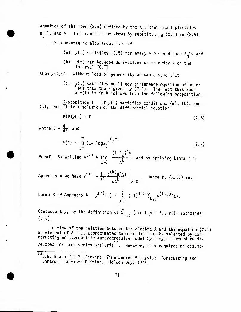
Proposition 1. If y(t) satisfies conditions (a), (b), and (c), then it is a solution of the differential equation

P(D)y(t) = 0 (2.6)

where D = ^ and

m n.+l P(C) = n (^ logX.) J

j=l -^

Proof: By writing y^"^^ = lim ^ A^ A'^

(2.7)

and by applying Lemma 1 in

(k), Appendix A we have y^^^ = l^ ^ JiiAl

dA' A=0 Hence by (A.10) and

Lemma 3 of Appendix A y^'^^t) = I (-1)^""^ S .y^'^"^^(t) j=l k,j

Consequently, by the definition of S, (see Lemma 3), y(t) satisfies (2.6). '''

In view of the relation between the algebra A and the equation (2.5) an element of A that approximates tabular data can be selected by con- structing an appropriate autoregressive model by, say, a procedure de-

veloped for time series analysis^^. However, this requires an assump-

13 G.E. Box and G.M. Jenkins, Time Series Analysis: Forecasting and Control. Revised Edition. Holden-Day, 1976.

11

tion of stationarity or else instead of the original data, say x(n),

n=0,l, ...,N, one must approximate differences A x(n) of order d that are assumed to be stationary. However, this assumption need not hold for tabular data that must be differentiated. For instance, if the under- lying function is exponential the differences of any order are exponential and hence non-stationary. An example of this type of data is a concen- tration of injected drug in blood measured as a function of time after injection. In view of this, instead of attempting to determine the order of differences that may produce stationary series and at the same time considering possible periodicity ("seasonal" variation), we choose a direct method for estimating the coefficients of an autoregressive model. To this end we write x(n,p,q) for x(p+qn) where q is any positive integer and p=0,l,2,...,q-l,n=0,l,...,Np, where Np=[(N-p)/qJ is the largest

integer not exceeding (N-p)/q. Let y(t)eA be an approximating function of the data, i.e.

x(n,p.q) = y(rA) + e^, (2.8)

where r=p+qn and e is an observation error assumed to be weakly sta- ^ 2 tionary white noise with zero mean and variance a . The function y(t)

satisfies (2.5) for a suitable polynomial P, say, of degree k since y(t)eA. We write this equation as follows

k y(rA) = I a. y[(r-jq)A] , (2.9)

j=1 ^

where the a.'s remain to be determined. By substituting (2.8) in (2.9)

we get k

x(n,p,q) - e = I a. [x(n-j,p,q) - e .]. (2.10) r j.^i J r-j

By transposing the terms in (2.10) and squaring both sides we get:

k x(n,p,q) - i a. x(n-j,p,q)

L j=l ^ -"

= e^ + I a^ e^ . + P , (2.11) r >. 1 r-1 r ' ^ '

j=1 J r-J

where P is a linear combination of products e e with u^ v. Since

by assumption e is white noise, we have E(P )=0. Thus, by taking

expected values of both sides of (2.11) we get:

72

x(n,p,q) - I a. x(n-j,p,q) j=l J

j=1 ' (2.12)

We replace the expected value of the left hand side by its estimate (average) and get:

q-1 N.

i I I N p=0 n=k+l

r ^ -1 x(n,p,q) - I a. x(n-j,p,q)

L j=l ^ J

j=l J

q-1 where N = I (N - k) . Thus we get from (2.13):

p=0 ^

(2.13)

a

1 q-1 N_ ~ 1 _

p=0 n=k+l H 1 i^ x(n,p,q) - I a. x(n-j,p,q) -" - ' 'iL . - 1

T2

J-1

j=i ^

(2.14)

We choose the estimates of the a.'s that minimize the variance a^.

These estimates are obtained by the following iterative procedure. Let

a denote the vector (a^). Assume that the value of a, say a^"^,has

been obtained on the u-th iteration. By substituting this value in

(2.14) we obtain an estimate a of the variance of e . Substitution of

this value for a in the second term of the right hand side of (2.13) yields:

q-1 \ I I

N p=0 n=k+l L

1 k -.2 x(n,p,q) -la. x(n-j,p,q)

j=l

- a k „

j=l ^ (2.15)

13

The next estimate a^" ' of the vector a is obtained by minimizing the right hand side of (2.15). Partial derivatives of this^expression with respect to the a.'s when set to zero and multiplied by N/2 yield

J

k q-1 P ~ 2 I a^A I I x(n-j,p,q)x(n-i,p,q) - N a a.

j=l "J p=0 n=k+l

q-"" ^P . ^ ! ■ ^ (2.16) = I I x(n,p,q)x(n-i,p,q) , p=0 n=k+l

i=l ,2,... ,k. Thus, if M is the matrix of the normal equations of the overdetermined system

k I a. x(n-j,p,q) = x(n,p,q), (2.17)

n=k+l,...,N , p=0,l,... ,q-l, and X is the right hand side vector of P (u+1) ... 2 .

these normal equations, then the vector a^ ' that minimizes a in (2.15) satisfies the equation

(M - N a/ I)a('''^) = X. (2.18)

where I is the k X k identity matrix. Successive iterates of the vector a

are obtained by substituting o^^ = 0 in (2.18) and then by iterating

(2.14) and (2.18). Thus, we need to obtain the normal equations of the overdetermined system (2.17) and then solve the linear equations (2.18).

In order to compute the a.'s by this procedure we have to choose J

k and the integer q in (2.17). Obviously a larger number of model parameters, i.e. larger k, yields a model better matching the data. A smaller value of q provides a larger number of data points, i.e. describes the structure of the data more accurately. However, in- creasing k as well as reducing q makes the system (2.18) ill conditioned. Hence the value of k and the data spacing parameter q must be chosen to

minimize a in (2.14) and at the same time to prevent the matrix in (2.18) from becoming nearly singular. Thus, we have two conflicting criteria for selecting* the optimal pair (k,q). As usual, a measure

This is similar to the solution of the numerical differentiation prob-

lem by regularization where increasing the regularization parameter reduces ill-conditioning of the problem and decreasing the parameter yields a better fit of the data.

14

of optimality must be chosen heuristically. Our choice is an index

J(k,q) = a^(k,q)/[D(l<,q)]^ , (2.19)

where D(k,q) is the absolute value of the determinant of the last itera- tion of (2.18) corresponding to the choice of k and q. Thus, we compute the ays and J(k,q) for k=l,2,...,kQ and q=l ,2 q^ and select the

pair (k,q) and the corresponding a.'s that minimize J(k,q). We impose

an additional constraint on (k,q) in order to prevent a choice of a model for which the data are inadequate, i.e. a model that contains terms of higher frequency than can be determined by the frequency of the data points. Thus, if w is the maximum frequency of the selected

model then we must at least have

q A <^ (2.20) in

Suppose further that for some q the coefficients, a.'s, in (2.17) yield

a real negative eigenvalue, say A. < 0. Then the term c.„ A" in (2.1) I in ^ jO J

is equal to c.„ |A | cos nir for every n. The frequency of this term

is IT radians per qA sec or ir/qA radians per sec, i.e. we have w >rr/qA, m

contrary to requirement (2.20).

If for some k and q the equation (2.17) has an eigenvalue with a negative real part, say A. = -a+ib (a>0), then the corresponding term

c.Q A, in (2.1) is expressible as C.Q exp(pn+iwn) where cos w = -a/A +h

i.e. w > -^ if expressed in radians per unit time equal to qA sec. There-

fore this choice of q yields a spacing qA with less than four data points per period of the corresponding term in (2.1). Although theoretically two points per period may be adequate to determine the real and imag- inary parts of the corresponding eigenvalue, even three points per period are inadequate when the data contain measuring errors. Further- more, a negative real part only implies that the corresponding frequency is greater than Tr/2 per unit time. It may also be greater than IT and less than 3TT/2, in which case the spacing qA provides less than two points per period. This is the reason why the pairs (k,q) leading to complex roots with negative real part are rejected.

In summary, the models (2.17) are determined for q=l ,2,... ,q„,

k=l,2,...,kQ and among those with eigenvalues having non-negative real

components that one which yields minimum J(k,q) in (2.18) is selected.

15

2

When the data is very noisy this selection of q may lead to a rather large step size qA and, thus, may eliminate high frequency terms present in the data even if the original spacing A is adequate to repre- sent this high frequency. This may happen when the amplitudes of high frequency terms are too small relative to the measuring error e to

be determined by the data taken at any spacing A. The procedure de- scribed above is intended to determine only the terms of (2,1) for which both the spacing and also the accuracy of the data are adequate, and this works satisfactorily in practice.

2.2 Smoothing and Differentiation

The procedure just described determines the coefficients a. in

equation (2.9), i.e. determines the structure of an element of A that minimizes J(k,q). The corresponding element of A is then given by (2.1),

n.

i.e. by y(t„ + nqA) = I I c. n y., where the y.'s are the roots u j=l i=0 ^^ ^ ^

°' . k , . U = I a.y^-J (2.21)

j=l J

of multiplicity n .+1. By reverting back from qA to the original spacing

A of the data and by writing A. for \i.'^ we can write (2.21) as follows: vJ J

n. m j I I o,y A^ = x„ , (2.22)

j=l i=0 Ji J u

where c.^. = c../q , u = -^ , and y(tQ+t) is replaced by the data value

x^=x(tQ/A + t/A).

The coefficients in (2.22) are selected to minimize the RMSE of the resulting approximation. This may be either a global or a local approxi- mation over the span, say, from u = -K to u = K. In the latter case the coefficients c.. are obtained by the least squares method from

(2.22) with u = -K, -K+1,..,K.^ The corresponding normal equations are

i+a ,u ,u V ,. .a ,u K m n .

,1 I I I

u=-K j=l i=0

or in matrix notation

S C = Z. (2.23)

16

Here S is a kxk matrix (k = j (n.+l)) with elements

K .^^

^zv " ^ " ^i ^R' i=0.1 .--..n.; j=l,2,...,m; a=0,l,...,n„; u=-K j 3

3-l,2,...m. C and Z are column vectors with the components c. and K J' V ct u 1 x^ u Ag, respectively. From (2.23) we get

C = S"^Z. (2.24)

Let A be a column vector with components v^X^. Then substitution of C

from (2.24) in (2.22) yields a smoothed value of x

T -1 Xy = A' S 'Z . (2.25)

Let Y^ be the column vector with components u°'\^. Then replacing Z in

(2,25) we get:

K J ^ \ = I X A' S"'Y, (2.26)

where A^ s'ly depends only on the x 's, u and v but not on x , i.e.

(2.26) provides a smoothed value of the data point x as a linear com-

bination of the data values x^. If (2.26) is used to compute the

smoothed value at the midpoint of the span of the data from -K to +K,

(i.e. XQ, then the weighting factors remain constant as the span, to-

gether with its midpoint, is translated along the axis of the independ- ent variable t.

The vector C given by (2.24) can be used to compute derivatives of tabular data. By differentiating (2.1), rescaling the independent variable t as in (2.22), substituting C from (2.24), and interchanging matrix multiplication and summation we obtain the following expression for the derivative:

1 K J r.-^ <~-'^X,'u'^' 'u (2.27)

where A^ = -^ is a column vector with components {u\^. log X.

+ iu^-^A^^)^ i=0,l....,nj, j=l,2 m.

17

Similarly, higher derivatives are obtained by the formula

where A

;;(P). i_ y'

. £A duP *

\ 'I '~''u (2.28)

Weighting factors in a formula like (2.28) for derivatives of various orders can be obtained directly from the structure of the data defined by the eigenvalues of a corresponding autoregressive model without computing the vector C in (2.24). Such a procedure is espe- cially convenient when all the eigenvalues are simple, and this case is described in Section 4.

3. DERIVATIVES AS LINEAR COMBINATIONS OF FUNCTIONAL VALUES

It was mentioned in the introduction that all the common methods for numerical differentiation express derivatives as linear combinations of discrete functional values in the form

y (t) k

I i = l

a^.y[t+(p-i)A], (3.1)

where p is some integer and A is the spacing between data points used. Various methods apply different criteria by which the coefficients a.

in (3.1) are selected. A generalization obtained by identifying a set, say A, of relation such as (3.1) and by defining a

of all these methods could be functions that satisfy the set of criteria for selecting

the coefficients. This we do below and in Section 4.

Obviously, any function that has a derivative at at least one point satisfies (3.1) for at least one value of_t. Therefore we restrict the set A by insisting that every element of A satisfies (3.1) for all t's in an interval such as [0,T]. If we allow the coefficients a. to vary

with t in a different fashion for every function in A,_then every dif- ferentiable and non-vanishing function in [0,T] is in A, since we can write f (t) = [ f (t)/f(t)] f(i) which is a special case of (3.1). Therefore we define the set A as a set of functions y(t) each of which satisfies t.

(3.1) with a.'s dependent only on y(t), p, and A but not on

We choose in (3.1) p=k+s+l and replace the summation index i by -j+k+s+1. This yields

k+s / (t) = I a(j,s) y(t + jA), (3 2)

j=s+l

where a(j,s) = a_j^^^^^^. Thus, the set A is defined as a set of

A: The following proposition is implied by Lemmas 4 and 5 in Appendix

_ Proposition 2. A = A, where A is the algebra generated by alge- braic, trigonometric, and exponential polynomials over the interval L'J»' J •

Proof: First we show that X c A. To this end we choose s=-l in (3.2) a na wr1te

k y'(t) = I b^l^ y[t+(j-l)A] , (3.3)

j=l ^

where b^^^^ = a(j-l, -1). We observe that

y^^^(t) = J b.(qV[t+(M)A], (3.4)

for q < k and some constants b^^^^ This relation is proved by induc-

?5°;^°[; ^'. L"^^^^' f^-"^^ ^°^^' ^°^ ^=1 because of (3.3). Suppose (3.4) holds for q < k. Differentiation of (3.4) with respect to t yields:

y^'"'^ (t) = I b/q)/[t.(M)A] . J . ^-vo w^. . (3.5)

?nSev'ftn ^ h f^ ^?[-^ '■" i^^^' ^'^ ' - -^-1 ^"d ^^^"Se the summation index J to u-h-1. This yields

k y'(t+hA) = Z a(u-h-l, -h-l)y [t + (u-l)A]. (3.6)

u=l

It follows from (3.5) and (3.6) that y^P"^^^(t) =

I b/q^^) y[t.(j-l)A], where b (^^1) = J b (q)a(j-u, -u), i.e.

19

(3.4) holds for q+1 and consequently it holds for q=l,2,...,k. Let B

be the kxk matrix with q^^ row (b^ ^^^b2^'^^,... .bj^^'^O • If B is non-

singular then we have from (3.4):

y(t) = I cy(J)(t). (3.7) j=i ^

where the c.'s are the corresponding elements of B" . If the rank of B

is less than k, then there exist constants d^ ,d2,... ,d|^, not all zero,

such that

q=l ^ J 0. (3.8)

j=l,2,...,k. Hence it follows from (3.4) that

I d^ y^^' = 0. (3.9) q=l q

Consequently y(t) e A satisfies either (3.7) or (3.9) and hence y(t)eA,

i.e. AcA.

The converse inclusion AcA follows from Lemmas 4 and 5 in Appendix A. Indeed, let y(t)eA, i.e. let y(t) be of the form (A.20) as in Lemma 4. The lambdas in (A.20) define the matrix L of Lemma 4. By Lemma 5 det L ^ 0. Hence there exists a unique solution vector b of equation (A^21) in Lemma 4. Consequently, y(t) satisfies (A.22) and hence y(t)eA, i.e. AcA. This completes the proof of the proposition.

Thus, if we either assume that tabular data can be approximated by an element of A, or that the derivative of the corresponding function can be expressed as a linear combination of certain data values, then in view of propositions 1 and 2 an approximating element can be ob- tained by constructing an appropriate autoregressive model such as (2.8) in the preceding section. In other words, the method described in the preceding section yields the exact derivative for a function in the set A=A, or, equivalently, in the set of functions that satisfy a family of difference equations of the type (2.4).

4. DERIVATIVES WITH SIMPLE EIGENVALUES

Equations (A.21) and (A.22) in Appendix A yield derivatives of tabular functions representable by autoregressive models, including those with simple eigenvalues. The needed weights b. in (A.22) are

20

obtained by solving the linear system of equations (A.21), This re- quires complex number arithmetic since the coefficients in the equation (A.21) are imaginary for imaginary eigenvalues >...

A closed form expression in terms of components of complex eigen- values can be obtained for the case of simple characteristic roots. An element of A corresponding to this case is

y(t) = I c.x] , (4.1)

i.e. it belongs to the subalgebra of A generated by trigonometric and exponential polynomials. The case of simple eigenvalues is of practical interest for the following reason.

Equality of two eigenvalues defines a functional relation between the Sj's, the coefficients of the corresponding autoregressive model, i.e. n defines a hypersurface in the k-dimensional Euclidean space

X^ of a^,a^,...,a^. Thus, the set of vectors a in X^*^^ that define

multiple roots has Lebesgue measure zero. Therefore if we assume that

experimental data yields points of aeX^ \ all equally likely in a finite region, i.e. with probability distribution proportional to the Lebesgue measure, then the probability of obtaining equal or nearly equal eigenvalues is very small, although synthetic data derived from algebraic polynomials does yield multiple roots.

In order to obtain a closed form solution of equation (A.21) we need the following lemmas.

_ Lemma 6. Let V^^^ be the Vandermondian of XQ,X, ,X2,... ,x and

V^^'^'' be its minor corresponding to the element x^. Then

V ^j) = S . V ^"^ , (4 2) n n-j n ' \'*-<^)

where S . is the symmetric function of x,,x,,...,x of order n-j and (n) . '^ \ d n

V^ IS the Vandermondian of X, ,X2,... ,x.

Proof. By expanding V^_^^ with respect to the first row (the row con-

sisting of powers of XQ) we get

n . . , .V

V , = y (-1 ^•^ X '^ V ^•^^ n+1 j^Q ^ ' ^ ^0 ^n •

21

Divide both sides by (-1)" V^^"^

n "^ n

r \ Since V^ is itself a Vandermondian we have

/ N n j-1 n J-1 v^^"^= n n (x.-x.). Also, v„,, = n n (x.-x.). " 3=2 i=l ^ ^ " ' j=l i=0 ^ ^

Therefore we get from (4,3)

j=l ^ ^ j=0 ^ V„^"^

V ^J^ (4.4)

The right hand side of this identity is thus a polynomial in Xg of

degree n with the roots Xi,Xp,...,x , and the coefficient of XQ is

equal to one. Therefore the coefficient of x^'^ is (-1) ""^ ^n-i' '^^^^>

we have from (4.4) S _. = V^^"^Vv^^"^ which is (4.2).

Lemma 7. Let S. be the symmetric function of X,,X„,...,X. of

order i and S.^^^ be the symmetric function of X, .Xp" • •'''^n.i'-^^n+i >• •-.X.

of order i. Then

S>^ = I (-1)^" S. .xj . (4.5) T j=o ^"-J P

Proof by induction on i. For i=0 (4.5) is an identity 1=1. Suppose (4,5) holds for i < k. The function S.^-, can be expressed as the sum

of all the products of i+1 factors taken from X, 5X2,.. ,X, ,X •,,... ,X.

plus the sum of all the products of i factors taken from the same set

with each product multiplied by X , i.e. S.^-, = S.^-,^'^' + S.^'^'X or

S.^T^P^ = S.^T - S.^P^X . By substituting S.^P^ from (4.5) we get 1+1 1 +1 1 p "^ ^1

22

u=l

i+1 i_u+i> - JQ (-^)"^-+l-u^p- This is the A "i+1 "i+1

relation (4.5) with i advanced to i+1 and the proof is complete.

When all eigenvalues are simple equation (A.21) is of the form

;A. s+1

' xJ''

s+2

s+2

s+k\ ^1

..X, s+k i

/'h\ /i°g^i\

I ^2! P°9%i s+l s+2 s+k

(4.6)

\h k \log^,

where A is the spacing used in determining the X's (i.e., q times the original data spacing). The solution b of (4.6) is obtained by Cramer's rule. This allows us to cancel common factors in the numerator and denominator that are differences of eigenvalues and, hence, to reduce the round-off error.

The determinant of (4.6) can be written as follows:

det L = s^^^ V = n x^^^ n [x.-x.) J>i

Let

and

Q(Ap)

P{X)

I7P

k

1 a. j=0 ^

k-j

(a^^ = -1) be the characteristic polynomial of (3.1)

Therefore

Then

9A

k =- n (X

x= x„ j=i P ^j)'

J7P

Q(Apj I (k-j) a.X^k-J-^ j=0 J P

or

14.7)

(4.8)

(4.9)

(4.10)

23

q(Xp) y q a, X q-l (4.11)

By writing n (X.-X.) = n (X^ - X.) n (X. - X.)(-1) "^ and by j>i ^ ' i=1 P ^ j>i J ■■ i=1 P

I7P i.J?'P

observing that the last product is a Vandermondian of X,,X^,...,X , ^ / \ I c p-I

X -,,...,X,, say V, -i , we can write (4.7) as follows:

,k-p <- s+1 (P) det L= {-^r^S^-' Q(X ) V^_/^^^ (4.12)

Continuing the application of Cramer's rule, let B. be the matrix j-s

obtained from L by replacing its (j-s)-th column by the right hand side of (4.6). By expanding det B._ with respect to this column we get:

(4.13)

where

det B =-^^1^ I (-I)P log^ •^ ^ A"^ P=I f

s+1 -s-1 (J-s-1), , ^k ^ Vi ^p)'

Vk.i^'"'-^^(P)

1 X.

1 X.

> J-s-2 , j-s ■^1 ^1

1 X ....xJ-^-2 X^-l p-1 p-1 p-1

' Vi'" P+1 X

,J-s-2

,X

X

k-1 1

k-1 P k-1 J-s

p+1 ''p+l

•^r^ 4"--A''

(4.14)

i.e. V^'^"^" ■'(p) is a corresponding minor of det B. divided by K-I J-s

^s+1,-s-1 \ ^p ■

Determinant (4.14) is a minor of a Vandermondian in X^,X,,...,X ,,

X i,...,X|^ corresponding to the (j-s-l)-th element of the first row.

Thus, by Lemma 6 above we have:

24

V (j-s-1), X ^ 3(p) ^(p) 'k-1 (4.15)

where S^P{. is the symmetric function of order k-j+s in Ai,Xo,...,

X 1 ,A 1,... ,X|^ and V|^_j is the Vandermondian of the same arguments

By substituting (4.5) in (4.15) we get

k-j+s <r^'(p) = v(p] i (-')'s,.j,3.„x

v=0

Since S. is a symmetric function of the roots of (4.9) we have

^k-j+s-v ^ '^ ^k-j+s-v '

By substituting (4.15) - (4.17) in (4.13) we get:

1 k / .^\} . „r, ^s+1 ,-s-l,,(p) ^^+ D ' V (-U log A S, A V, , det B = — ^ ^ ' ^ P k P k-1

^ ^ A"^ P=1

V"' ( i^k-l \lo ^-'^ Vj+s-v^p •

In view of (4.11), (4.12), and (4.13) Cramer's rule yields:

k-j

1 i 'P '"' 'P vL '^-J ■■ ' b. = ^ y J A-" p=l

v V -p

1 vA„ a, v=i P k-v

(4.15)

(4.17)

(4.18)

(4.19)

Formula (4.19) provides a closed form expression for the coefficients in (3.2) in terms of the coefficients a of the autoregressive model (2.9)

and in terms of the eigenvalues of the corresponding difference equation. Since some of the eigenvalues may be imaginary, computation of the b.'s

by (4.19) still may require complex number arithemetic. This can be avoided by combining complex conjugate terms in (4.19).

* * * Let (A|,Xj), (A^,A^ )>• • • >(^^J.A^) be the pairs of complex conjugate

roots and ^2u+l'"'"''^k ^^ ^^^^ ^°°^^ °^ ^^^ characteristic polynomial.

25

Write (4.19) as follows:

1 "

-s r h^ X„ log X y a. . XV

P P v=0 ^'^'^ P * y + j k

I v=l I ' ^k-v ^p

1

k-j ^n^ log'' A„ y \ . y X D ^ D ^- k-1-V

^T ^ k A"^ P=2U+1 ^

v=0 k-j-v >

v=l '^

where T^ is obtained from the first term in the brackets by replacing X by X . By adding the terms in the brackets we get

r r

(•

k-J k *v / *-s , * k-j

P ^^0 k-J-' P/v=l ' P : I I d„x +|x Vv=l ' P \

^^°9 ^, 1 a, . X 1 Id^X^ +h log^, I a v=0

(J,'.':)(J.'-':') (4.20)

where d^ = v a^_^ .

The denominator D of the last expression can be transformed as follows;

"p ' X "''VP*'" ' ,1 '^Vn' (\\ * Oo )

By writing X = A +iB , a = log |X |, and 3 = arctan B /A we get

k k (v+n)a D = y f e '^ cos P v=l n=l

r (v-n)3 I d„d L ^ ' pj V n

Similarly, the numerator N of (4.20) can be transformed into r

26

k-j k I . j-^ ^p = 2 ); I ^k-i-v ^n exp (v+n-s)a + r log /a_ +

P v=o n=l '"^-J- P ^P

cos (v-n-s)3 + r arcsinfg yVa^+3 ^

Neither N nor D involves any imaginary elements.

Consequently, we get:

1 u N^ , k

^ A p=l ^p A"^ P=2U+1

^ -s 1 r , '^v^ ,v ^r. log K } a^ • ^ P ^ P ^Q k-j-v p

k r V a

v=l k-v^p

(4.21)

a closed form solution for the coefficients in (3.2)

5. ERROR BOUNDS

In this section we develop expressions which yield approximate bounds on the errors in derivatives calculated by the method of Section

Let x^ = x(t), t=0,A,2A,...,nqA be tabular data of a function

y(t) eA with the measuring error e., i.e.

x(t) = y(t) + e^. (5.1)

We assume that e^ is a white noise with zero mean and variance a . As

shown on the preceding pages the r-th derivative of y(t) is expressible in the form

^^''^(t) = r b. (rj y(t+jqA). (5.2) j=s+l J

and its approximation x^""^ (t) is

,(r), k+s

x^'Mt) = I b (r) x(t+jqA). j=s+l -J"^

(5.3)

27

where the b. 's are expressed in terms of the coefficients in an auto-

regressive model

k . x(t) = I a. x(t-jqA) (5.4)

corresponding to the difference equation

' k y(t) = I a. y(t-jqA) (5.5)

satisfied by the function y(t). Let

df''^ (t) = x^''^(t) - y^'^^t) (5.6)

denote the error of the approximation. Since the coefficients b. j ~ -^

are functions of tabular data, we can use the relations (5.1)-(5.5) to

t) < :(r-),

(r) express 5^ '(t) as a function of x(t),t=0,A,..., and, thus, obtain the

variance of 6^ '(t) expressed in terms of statistics of e.. This yields

a measure of the accuracy of numerical derivatives obtained by the method described in the preceding sections.

In the present section we derive an approximation to the bound of (r)

the variance of 6^ (t). To this end let

Bj_s = b._3(r) - b._3(r) . (5.7)

i.e. 6- c is the error in the estimate of b. (r). In order to simplify J--^ J-s

subsequent algebraic expressions we assume that the estimates b. (r)

are unbiased, i.e.

E (B 3) = 0. (5.8)

By substituting (5.2) and (5.3) in (5.6) we get

:(r),

where

6^'^^(t) = A^ + B^, (5.9)

k+s

28

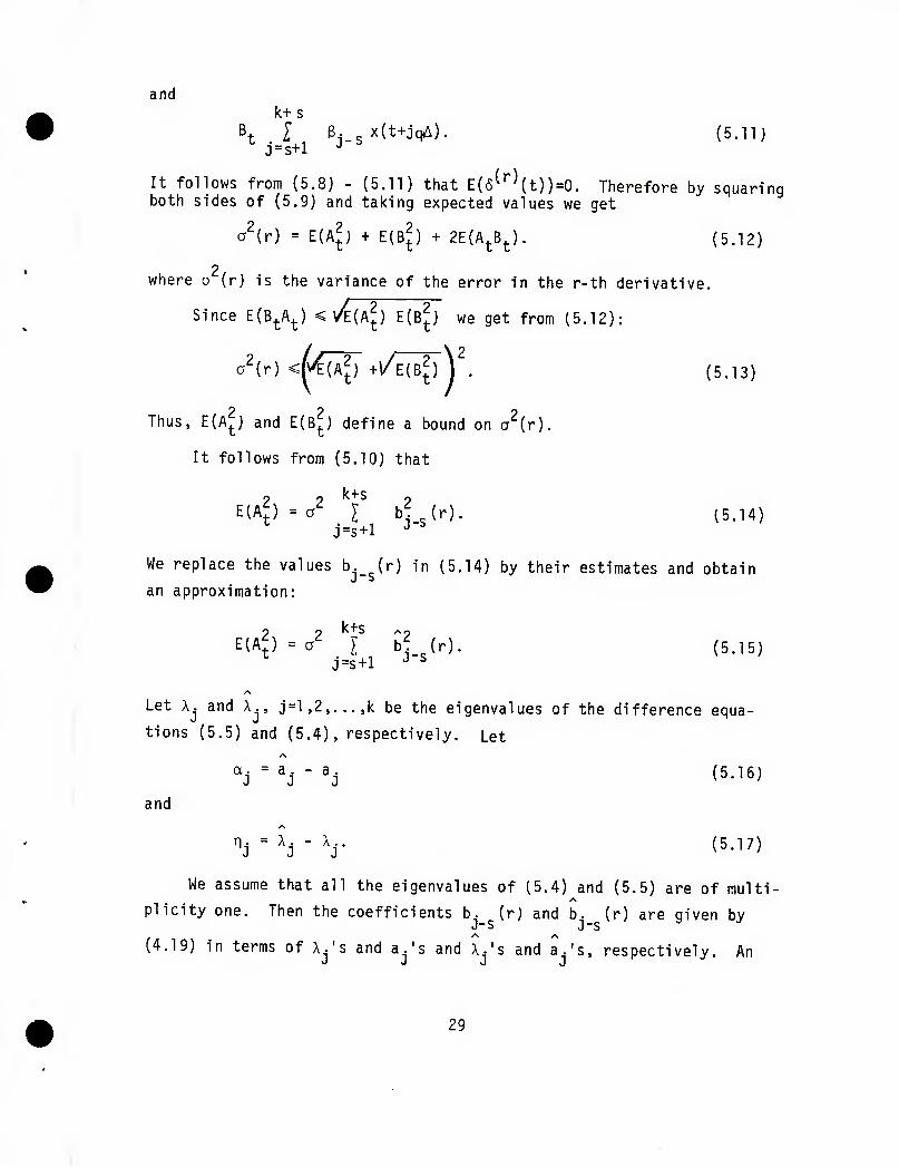
and k+ s

j = s+l ^ (5.11)

(r) It follows from (5.8) - (5.11) that E{&^^'{t))=0. Therefore by squaring both sides of (5.9) and taking expected values we get

a^(r) = E(A^) + E(B^) + 2E(A^B^). (5.12)

where a (r) is the variance of the error in the r-th derivative.

Since E(B^A^) < /E(A^) E(B^) we get from (5.12):

2 o^ir) /v/E(Af7+\/E(B|y y (5.13)

Thus, E(A^) and E(B^) define a bound on a {r).

It follows from (5.10) that

o o K+S rt E(A^) = a' I b^,(r).

j=s+l ^"^ (5.14)

We replace the values b._ (r) in (5.14) by their estimates and obtain J ^

an approximation:

o , k+s E(A;) = a^ I

j=s+l ^j-s^^)- (5.15)

Let Xj and A., j=l,2,...,k be the eigenvalues of the difference eq

tions (5.5) and (5.4), respectively. Let

ua-

and "j = ^j ■ ■'i

/\

'r'r - X. J

(5.16)

(5.17)

We assume that all the eigenvalues of (5.4) and (5.5) are of multi-

plicity one. Then the coefficients b. (r) and b. (r) are given by J-s j-s

(4.19) in terms of A.'s and a.'s and A.'s and a.'s, respectively. An J J J J

29

expression for B. in terms of the a.'s can be obtained from (4.19),

(5.7), (5,16), and (5.17). This is a non-linear algebraic function. We approximate this function by the following linear relation

k+s k d6. B^ = I x(t+jqA) I -^ a. or

j=s+l i=l ""i

k k+s d3,- K K+S ap-

^ i=l ^ i=s+l ° ^i (5.18)

where

dB ill.

d3 da.

ill da.

'i=0

k 3B.

p=l 9X„ P P

5 8a. a

i=0

and 9B-

da 2

3B J-s da

^i=0

'i-0

9B-

da a .=a •

1 1

(5.19)

In order to simplify further derivation of an expression for E(B^ ) we

introduce the following notation:

Np = A- log-- Xp.

^p"- ii" 'p '^-"'

N(j.p) = N N . , P PJ

(5.20)

(5.21)

(5.22)

(5.23)

and

ffX A A a a a ) = ^(J'P) (5.24)

30

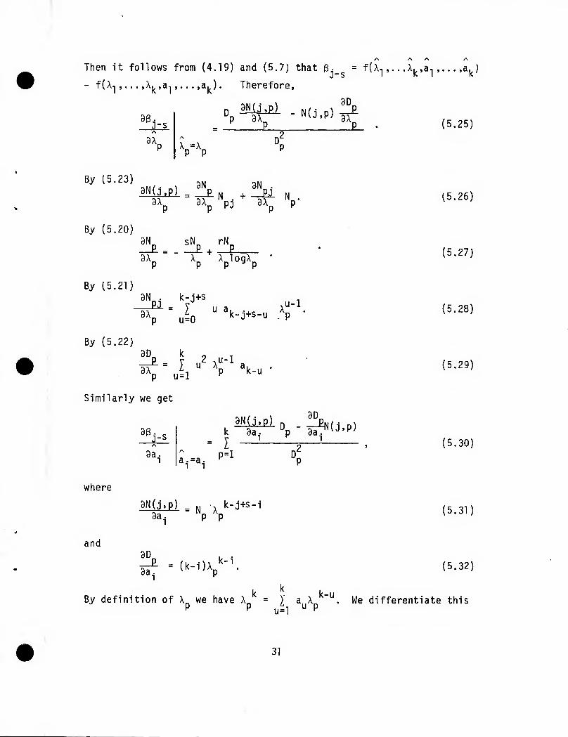
Then it follows from (4.19) and (5.7) that g. = f(XT,. J-s I

f(Xl ,... ,A|^,a^,.. .,a|^). Therefore,

3D.

9A_ p e_

P P

■\'^1 ^k^

(5.25)

By (5.23)

9X„ 3X„ 'pi 9X ' p- p p ^"^ P (5.26)

By (5.20) m sN rN

P P P ^ P (5.27)

By (5.21) 8N . k-j+s

X u-1 (5.28)

By (5.22)

p u=l

Similarly we get

'6j-s

p V 2 ,u-l TTT^ = > u X a, 8X_ ^, p k-u

9D.

3a. a .=a. 1 1

k^o^->^-'P) I — r^

P=l D„

(5.29)

(5.30)

where

3N(j.p) ^ ^ . k-j+s-i 3a. - % ''p (5.31)

and 9D

9if = (^--^^p k-i (5.32)

k k-u By definition of X we have X = I a X . We differentiate this

31

expression with respect to a. and solve the resulting equation for 8Xp/3a.:

9X

3a. ^ ^p -/ kA„ - I (l<-u)a^X J.

u=l L P (5.33)

The formulas (5.19) - (5.33) define the coefficients d3._ /da. in (5.18)

and, thus, the quantities C. in the following:

k+s d3. S = ^ ^ii^ x(t+jqA) (5.34)

k k Je have by (5.18) B. - ^ C a.. Hence B/ = ^ ^ %«v^u^ ^""^

^ 1=1 ^ ^ ^ v=l u=l " " ^

E(B^2) ._ E^[E(B/|t)] = E^ r k k

y y C C E(a a |t) ^, ^1 u V ^ u v' ' v=l u=l

(5.35)

where the conditional expectation is over the distribution density func- tion of the a.'s. Since E(a a |t) does not depend on t we get

E(B/) = I I E(a„a^). E,(C„C„) - I I E{a„a,) • i I C„(t)C^(t) v=l u=l v=l u=l t

k k 1 y y y E(a a )C (t)C (t). N i: ^1 ^1 ^ u v' u^ v t v=i u=i

The quantity Ho in (2.17) is small as compared to the diagonal P ^

elements of the matrix M. Therefore the estimates a. in (5.4) differ

only little from the least squares estimates of the a.'s, and hence ■J 2 ~ 2 -1 _

the covariance matrix (E(a a,,)) can be approximated by a (M-Na I)

a M . By writinq m for an element of M obtained by estimating the ■^ ^ uv regression coefficients (a.'s) we have the following approximation:

J

E(B/) -^ I I I C^(t)C^(t)m ^ t u=l v=l ^ ^^

(5.36)

32

If Ap's and a.'s in the definition of C^^ are replaced by \ 's and

aj's, formula (5.36) yields an estimate of E(B^^). This together with

(5.13) and (5.15) defines an upper bound of the variance of the error in the estimate of the r-th derivative. However, this is not an absolute bound since its estimate depends on the assumption that (4.19) yields unbiased estimates of the b^'s, on the accuracy of linearized expressions

of bj's in terms of a^.'s and X^s, and on the effect of replacing a.'s

and Xj's by their estimates, a.'s and X.'s, respectively.

A few examples listed in Appendix B show that the formula (5.13)

yields reasonable bounds of a^(r) in almost all the cases tested and hence it can be used as an indicator of accuracy for the numerical esti- mates of derivatives obtained by the method of this report.

Further applications and examples will be presented in a companion report now in preparation. Additional sets of synthetic data as well as samples of field test data will be considered therein

REFERENCES

1. T.F. Dolgopolova and V.K. Ivanov, On Numerical Differentiation. Zh. Vychisi Mat. Fiz. 6, 3, 570-576, 1966.

2. R.S. Mderssen and P. Bloomfield, "A Time Series Approach to Numerical Differentiation." Technometrics 16, 1 69-75, 1974.

3. C. Masaitis, G. Francis and V. Woodward, "Survival vs. Horsepower per Ton Test Data Analysis," BRL MR 2518, 1975. (AD #00032111)

4. R.F. Lieske and A.M. MacKenzie, "Determination of Aerodynamic Drag from Radar Data," BRL MR 2210, 1972.

5. F. Yagi, B. Jansen, L.B. Kennedy, W.C. Taylor, "Analysis of Interferometer Records of Projectile Motion in the Bore of Small Arms," BRL Report 939, 1955. (AD #74976)

6. D.B. Hunter, "An Iterative Method of Numerical Differentiation," Comp. J. 3, 270-271, 1960.

7. A. Talmi and G. Gilat, "Method for Smooth Approximation of Data," Journal of Comp. Physics 23, 93-123, 1977.

8. H.C. Hershey, J.L. Zakin and R. Simha, "Numerical Differentiation of Equally Spaced and Not Equally Spaced Experimental Data," Ind. Eng. Chem. Fundam. 6, 413-421, 1967.

9. P. Craven and G. Wahba, "Smoothing Noisy Data with Spline Functions," Numer. Math. 31, 377-403, 1979. *

10. A.N. Tikhonov, "Solution of Incorrectly Formulated Problems and the Regularization Method," Soviet Math. Dokl. 4, 1035-38, 1963.

n. J. Cullum, "Numerical Differentiation and Regularization," Siam J. Numer. Anal. 8, 254-265, 1971.

12. R.S. Anderssen and P. Bloomfield, "Numerical Differentiation Pro- cedures for Non-Exact Data," Numer. Math. 22, 157-182, 1974.

13. G.E. Box and G.M. Jenkins, Time Series Analysis: Forecasting and Control. Revised Edition. Holden-Day, 1976.

34

APPENDIX A

Lemmas 1, 2, 3 below simplify proofs in Section 2, while Lemmas 4, 5 are found useful in Section 3.

Lemma 1. Suppose y(t) satisfies the conditions (a), (b), and (c) of Section 2. Let S (A) be the symmetric function of the roots of (2.4)

of order j and M.(A) = S.(A) - C^) . Let

N(A) = I (-l)J-l M,{A)y(t-jA). j=l J

Then

d^N(A)

dA^ 0 for q=0,l k-1.

(A.l)

(A.2)

A=0

Proof. With f(t) replaced by y(t) equation (2.4) can be written as follows by expanding P^, replacing powers of B , and solving for

y(t): k . .

y(t) = I (-l)J-^ S (A) y(t-jA) . (A.3) j=l ^

By substituting (A.3) into the identity

Nk. k . Ik\

(1-B^)>(t) = y^+ I {-^)^ L t(t-jA) we obtain

\j-lr (l-B^)V(t) = I (-l)J-'M.(A)y(t-jA)^ N(A). j=l ^

It follows from (A.4) that the k-th derivative of y(t) is

.<^'(t) lim N(A)

A-^0 A

(A.4)

(A.5)

Now we prove (A.2) by induction on q. Indeed, it follows from the def- inition of M.(A) that M.(0)=0 since each term of S.(0) = 1. Hence by

(A.l) N(0)=0, i.e. (A.2) holds for q=0. Suppose it holds for q=n<k-l. Then by applying L'Hospital's rule to (A.5) n+1 times we get

35

,(k)(„,„,d^%A)/dA^ A->0 k(k-l)...(k-n)A k-n-1

(A.6)

(k) By hypothesis (b) y^ '(t) is bounded. Therefore (A.6) implies that

d"^lN{A)/dA"^^ A-0

For

0, i.e. (A.2) holds for q = n+1 < k. Q.E.D.

J-1 n. and X. in (2.2) let m. = J (n.+l) and v _,, = v ^^ J J J ^^2 '^i i

= A.. Let T, . be the set of all the combinations of the integers J-+1 -J ^'^

1,2,...,k taken j at a time. Let M. = M.(A) J J

Lemma 2. Let

L. (i,,i2,...,i .) = I log v ^ ^ ^ J u=l \

Then

(A.7)

I (-1)^ jP I Lj-P (i,,...,i.) i=l T "^ -^ J

(A.8)

for p < q < k.

Proof. Differentiation of (A.l) yields

But

d^N(A) _ V I (-1)^'"^ k-y^^^t-jA) (-j)^

q-1 I (J) M.(^-P) y(P)(t-jA) (-j)P] . (A.9)

p=0

M.(q-P) = y A A A q-p , .

'k.j ^ '^ J

36

Thus,

d^N(A) I (-i)M V y^^ht) (-j)P A=0 j = l p=0

k,j ly (M.ij.. .,ij)

By interchanging the order of summation we get

d^N(A)

dA^ A=0 P= =0 \n 3=1

.1 iq-p

'k,j ^k (ii.i2'---'ij) (A.10)

It follows from (A.2) and (A.10) that

q-1

P

(A.11) k,j

for q < k,

Let PQ < q-1 be the largest value of p with non-vanishing coeffi-

cient of y(P) in (A.11), i.e. (A.11) can be written in the for )rm

p=0 P 0, an ordinary differential equation of order p.

ni "j whose solution y(t) is thus of the form y(t) =11 C..t''

j=l i=0 J^

^J^

37

m ^ with Pp, = I (n.+l). But it then follows that y(t) satisfies the

m y. P..+1 difference equation P(B)y(t)=0 where P(X) = I (A-e ^) ^ , i.e. a

difference equation of order p^ < q-1 < k, contrary to the assumption

(c). Therefore in (A.11) we must have

I (-l)JjP I LJ-P (i,,...,i.)=0, (A.12) i=l -p K. 1 j

for p < q < k, which is (A.8). Q.E.D.

Next we prove the following lemma, making use of the previous one.

Lemma 3. Let L (i^ ,i„,... ,i .) be as in (A.7). Then

\,u-M^ j (-!)¥- I L",(ii,i,,...,i.)^V (A.13) ^'^ 'k,j

for u=l,2,...,k, where S. is the symmetric function of C,-=log v.,

i=l ,2,...,k, of order u.

Proof. This lemma is proved by induction on k. When k=l the

right hand side of (A.13) is -^'{-l)•E,■^ which is S^ j. Suppose that

(A.13) holds for k-1. For any positive integer u, S. is a linear

function in each argument and it can be written as follows:

^k.u(^k) =^kVl.u-l-^ Vl.u ^"-^'^ for u=l,2,...,k (we assume that S, •, . = 0 and S,^ Q=1 for k > 1). Since

V in (A.13) is a symmetric function of the 5-'s, we need only to show

that V is representable in the form (A.14), i.e. that

38

and

(A.16)

We write (A.13) as follows;

^^^k^ " u:(k-u): k-1,1

Ci(^-) ^ ^l

+ (-1)" k}'-" L|;_J (i,2,....k-i)

* I <'-k-l('l-^2- •'j-l' * 5k' ■] Therefore,

V(0) = _M01 u:(k-u)

(A.17)

■ I L^_i(i) + (-l)^k^-"L"^_j(l,2,...,k-l) ^k-1,1

+ V (-1)^' J^-" I L" ,(1- ,1- i.

^"^ 'k-l,j-l

39

By changing the summation index in the last sum and by combining the terms we get

V(0)

We apply the

binomial theorem to the expressions in the brackets and get

^ ^"^ 'k-l,j

k-1 , k-u /k-u\ . . "J

K- i , J

By the inductive assumption the first term in the braces multiplied by

the factor outside the braces is S. , . We interchange the order of K-1,U ^

summation in the second term and get:

k-1 k-u /k-u

I i=2

V(0) = S, 1 + ^—r-r J \ i '' \u u!(k-u)! -tr, ^ k-1

k-1 \j .k-u-i I (-1)^ J^-"-^ I L^, ,(i,,...,i.)

k-l,j

By (A.8) the expression in the brackets is zero, i.e. V(0) = S, , k-l,u

Thus, (A.15) is proved.

40

I I

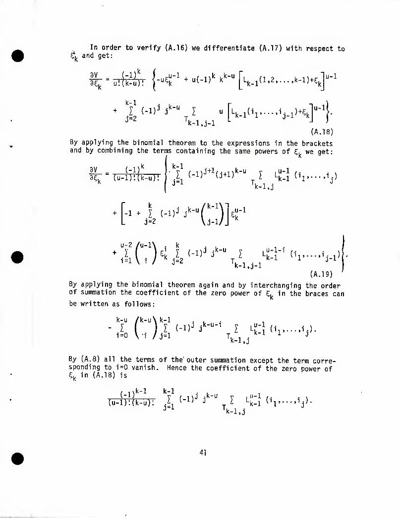
In order to verify (A.I6) we differentiate (A.17) with respect to ^1^ and get:

9V 95, J^ {-U5-1 . u(-l)k k^-" [4.^(1.2,...,k-lK u-1

k-1 + I i-iy

k

u-1

■^ 'k-l,j-l ^

(A.18) By applying the binomial theorem to the expressions in the brackets and by combining the terms containing the same powers of 5, we get:

(-1) )• V f nJ+l/.-4.nl<-u V ,u-l ,, 8V 3? -Mu-i];(k-u): •M-i)^--(J^i)--" I Ln(ip...,i

u-2 /u-l\ . k

i=l \ i / ^ j=2 T, , , , ^-1 1 J-1 I 'k-l,j-l

By applying the binomial theorem again and by interchanging the order of summation the coeff"

be written as follows:

(A.19)

of summation the coefficient of the zero power of E.. in the braces can

k-u /k-u\k-l II

i=0 \ i / j=l (-l)j j^-^-^' I L;;:} (ii,...,i.).

k-l.j

By (A.8) all the terms of the outer summation except the term corre- sponding to i=0 vanish. Hence the coefficient of the zero power of 5|^ in (A.18) is

k-1 k-1

(u-i):(k-u): ,V ^ T^ ^-1 (h"-"'j)- ^ 'k-l,j

41

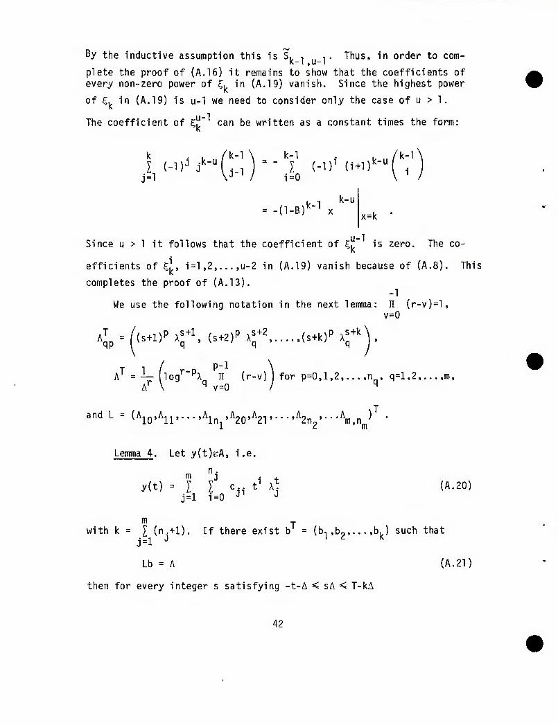
oy the inductive assumption this is S. , ,. Thus, in order to com-

plete the proof of (A.16) it remains to show that the coefficients of eyery non-zero power of L in (A.I9) vanish. Since the highest power

of E,. in (A.19) is u-1 we need to consider only the case of u > 1.

Th -u-1 e coefficient of 5^" can be written as a constant times the form:

k . . /k-1 k-1 I (-1)' (i+1)

i=0

k-u k-1

-d-B)''-'' X k-u

x=k •

u-1 Since u > 1 it follows that the coefficient of E,. is zero. The co-

efficients of E,'!, i=l ,2,... ,u-2 in (A.19) vanish because of (A.8). This

completes the proof of (A.13). -1

We use the following notation in the next lemma: II (r-v)=l, v=0

<p = ((^^l)'^r' (s-^2)Px^^^....,(s-Hk)Px^^^V

A^ = ^ (log'""Px n (r-v) ) for p=0,l,2,...,n , q=l,2,...,m, A \ ^ v=0 / ^

and L = i^lo>hv■^■'\'^ZO'h^'■■"^Zn^'■■^\,n/ '

Lemma 4. Let y(t)KA, i.e.

n . m J i .t y(t) = I I c . t' X

.1=1 i=0 J^ ^ (A.20)

m j with k = [ (n.+l). If there exist b = (b-, ,b,,... ,b. ) such that

.1=1 ^ 1 ^ K

Lb = A

then for ewery integer s satisfying -t-A < sA < T-kA

(A.21)

42

(r) ^'^^ y (t) = I b. y(t+jA). (A.22)

j=s+l J ^

Proof. Substitute (A.20) on both sides of (A.22) and equate the

coefficients of the terms t^A^ on the opposite sides of the result.

Then (A.21) is obtained. The lemma is proved by reversing these steps as follows. ^

The expression (A.21) is a system of equations

T 1 P"-'- ^p ^ =^log'"-P Aq ^n^ (r-v), p=0,l,... .n^, q=l,2,...,m or

k /. . .ND ,S+i . 1 - y-n i"-"-

(A.23) ; (s+j)PA^^n ^Vlog'-PA^ V (r-v) J = l ^ ^ A ^ v=0

For each q-l,2,...,m and z=l,2....,nq multiply the equations of (A.23)

corresponding to p=u-z (u=2.2+l,...,n ) by c (^) and sum on u. This yields

n

u=z "^^ \ ^ / j=i q j

9 /,.\ „ ,,., u-z-l 1 H / u \ r u+z u-z-l 7 uL 'qAzj^°9 " \ n (^-v)- (A.24)

v=0

write (A.24) in the form

n

'7L"^-'°' \(u-z) n (u-v). (A.25)

43

Now we multiply (A.25) by t^ and sum on z from 0 to n :

"q z /u\!< ,^. y t^ y c ( ) y (s+j)^"' x^^^ b.

q j=i

"q "q / r \ u-z-1

A z=0 u=z ^ H \ / y=o

We interchange the order of summation on both sides of this equality:

j=l ^ ^ u=0 ^^ z=0V^ /

"q u / \u-z-1

h^ u=0 ^ z=0 ^ V /v=0

Multiplication of both sides of this equality by A yields:

I b. { c x^^^-^J (t+s+j)" = { c,„^-(tV).

By summing both sides of this equality on q from 1 to m we get:

n„ "1 m q t+s+i II

j=l J q=l u=0 ^" ^

n

= y y ^- (c t%*). q=l u=0 dt^ ^" '^

^ fr) In view of (A.20) this is I b. y(t+s+j) = y^ '^(t) which is equivalent

to (A.22). n n "^ f +1 Hn +11

Lemma 5. Denote x\\\ = 11 jl, n:= I j, and P„ = n X. ^^^"j ". j=l j=l " j=l ^

Let the matrix L be as in Lemma 4. Then

44

m m n.: m j-1 det L = p II n.:: n X J n n (x.-x.)

"■ i=l ' 3=1 J j=2 i=l J ^

(n.+1)(nj+l) . (A.26)

^^^2£f- Let T. = y. g^ and T.P(X.)f(y.) = T.Pf(y.)

1 j

i.e. the result of the operator T.^^iX.) is obtained by applying the

operator T. p times and then substituting X. for y.. In particular,

TJ°^ (Aj)f(y^.) = f{Xj.). Let m^ = j (n.+l) and

T(p) = n n T, J"^ (X.) . j=l i^m.._-,+l ^ J

(A.27)

Let

* L =

s+1 s+2 s+k ■Ml

S+1 s+2 s+k

Then T(m)L = det L. This identity is used to prove the lemma by in- duction on n^., j=l,2,..,m. Indeed, if n^^O, j=l ,2,... ,m=k then by

(A.27) the operator T(m) = T(k) simply replaces y. by X., j=l,2,...,k,

i.e. the left hand side of (A.26) is a Vandermondian multiplied by

n s+1 k j-1 Xj ^"^ ^^^ '^^9'^^ l^^nd side reduces to n L n n (X -X )

J-1 j=l J j=2 i=l ^ J ^ '

i.e. (A.26) holds for this choice of n^.'s. By induction assume that

(A.26) holds for n^ .n^ n , with

"p+1 = "p+2 n = 0 m (A.28)

and np replaced by v such that 0 < v < n Under these assumptions (A.27) implies that ^

TCm) = T*(j,p,v) T(p,v), (A.29)

45

* where T (j,p,v) is an operator that replaces y. by X. ,, , for

J j-mp_^-v+p-l

j=m ^j+v+1,...,k and

T(p.v) = n ^- T(p-l), (^3^^

with T(p-l) defined by (A.27).

Let *, ^ P-1 P-1 n. : {n.+l)(n.+l)

p (p) = n n.:: n \.^ p^ ^ n (x.-x.) ^ ^

By induction (A.26) holds for the parameters in (A.28). Hence it follows:

T*(j,p,q) T(p,q) L* = P*(p)q:IXp^=X ^q+IJ^^+l)

n x^.^i n(x-x.)(q^i)("i^i) n(x. - xJ^^^ P+l ^ i<p P ' j>p J P

m

n,+l n ■ ^p

n (x.-x.) n (x.-x.) j>p ^ j>i>p ^ i<p-l

or

T*(j,p,q) T(p,q) L* = P*(p)q: IX^^ = X ^^"^ ^ ^^"^l) . r r

n.+l n ,, , v(q+l)(n.+l) *f . . ^ , , "i (A -X.)^^ '' ^ ' J (j,p,q) n (y.-X^)

<P j>ni„ ,+a+l J P-:

i<p-l

n (y.-^i) n yfi n (U.-A )^^^ J^i^f^p-i+q+i j>"ip_i+q+i j>p ^ P

(A.32)

46

Since T (j,p,q) has an inverse it follows from (A.32) that

P P u' P i) 'P

s+l j>i>mp_j+q+l J J>mp_j+q+l J J>Yi+q

i<p-l

n,+l

j>m n (y.-A ) q+l

(A.33)

Now let us apply the operator J^^^ (x ) to both sides of (A.33)

It follows from (A.30) that P-1

TSpl^+q.2 ^V^P'^^ =T(p.q.l). (A.34)

We^write the right hand side, say, R(p,q) of (A.33) in the following

where

R(p,q) = (y _x )q+lR (A.35)

Ri = P*(p)q;:A^q=A^(q+i)(s+i) n (A -A.)(^^i^("i^i) P P

" _(^J-!-lJ„, +n+9)

1<P

(y.-yjur^ J>%_l-q-2^^J ^%.l-q-2^ j>i>m _^.q.2^'r^J^^mp,^.q.2

TT S+l „ , "i+l n,+l

i>m +0+2 'J i<nl ^^"1 ^+q+2-^•) " (y -X ) ^ J>'"p-l+q+^ i<P-l p-l ^ j>m _^+q+2 J ^ P-

i<p-l

n (y.-Aj^^^ J>mp+i+q+2 J P (A.36)

47

Application of T^ ^ ^p ^° (A.35) yields a sum of terms containing p-1 ^

derivatives of (y , ^^-X )^ with respect to y ^ ^^ of orders mp_j+q+2 p' ^ ^mp_j+q+2

0 up to q+1. Thus, we can write

with derivatives of (y , .^-^ ) of order less than q+1. There- m i+q+i- p

where the second term on the right hand side is the sum of the terms

,q+i „p_^Hq+2 'y

fore by substituting y ^ ^^=X in (A.36) and in (A.37) we get •^ ^ m i+q+2 p p-1 ^

. n (A-A.)(^^i)("i^i) n (y.-xj n (yr^-)C^ i<p-l P ^ J>%_i+q+2 ^ P j>i>m ^^+q+2 J ' f'

c+1 "■,•"'■1 "i''"! n yf^ n (X-X.) ' n (y -x.) '

J>"ip.i+q+2 "^ i<p-l P J>nip_i+q+2 ^^

p- j>m^+q+2 J P

or n+1 (a+D- (q+2)(n.+l)

. n (y.-xj^^2 P*(p)x;^^^)(^^i) n (y.-X.)""' j>mp_^+q+2 J P P ■ j>mp_j+q+2 ^

i<p-l

48

• n (y -X ) q+1

n iu.-M.) n s+1

By comparing this with (A.33) we see that

^r^+q+z (^p)R(p.q) = R(p.q+i)

In view of (A.34) we have

T(p,q+1) L* = R(p,q+1)

(A.38)

(A.39)

By applying the operator T (j,p,q+l) to both sides of (A.39) we obtain (A.26) for n, ,n2,...,n ,, and n replaced by q+1. This completes the

proof of the lemma.

49

APPENDIX B

Details of the procedure for numerical differentiation according to the method of this report will be described in a forthcoming report that win contain examples of synthetic data as well as applications to experimental records. Here we include only a few illustrations that compare the accuracy of this method with the accuracy of moving polynomial arcs, Butterworth filter, and spline. These methods were selected for comparison because they are frequently applied to problems of interest to BRL. Furthermore, the corresponding computer programs are available. Also, spline approximation yields one of the most accurate, if not the most accurate, derivatives of all the commonly used methods for numerical differentiation. Comparison with Kalman filter is not included here since the results of this method are highly dependent on the assumed dynamics. If linear equations are assumed that are satisfied by a sine function of a given frequency, Kalman filter produces good results for the corresponding synthetic data. However, if the same dynamic model is applied to synthetic data obtained from, say, an exponential function, estimates of derivatives are poor. Illustration of these cases will be provided in the forthcoming report.

The synthetic data used here is described in Table 1. Here column 1 numbers the cases from 1 to 6 for convenience of reference. The corresponding functions x(t) are specified in column 2. The last case here is the Bessel function of the first kind of order zero. The values of the functions were computed at points in the intervals listed in column 4, and column 3 shows the step size for selecting the points in the respective intervals. Pseudorandom white gaussian noise with zero mean and the standard deviation a given in column 5 was added to each value, and then various methods for numerical differentiation were applied to the noisy data.

Table 1. Synthetic Data

1 Case

2 x(t)

3 A

4 I

5 a

1 sin 2TTt .004 [0,1] .02 2 sin 2Trt .004 [0,1] .05 3 e^ .01 [0,5] .01 4 4^(l+t+tSt'') .004 [0.2] .32 5 sin 27rt+.lsin lOTTt .004 [0.1] .05 6 J,(t) .01 [1.6] .01

51

The methods used are listed at the top of Table 2. Here moving polynomial arc corresponds to a cubic polynomial fitted to either 11 or 17 data points as indicated. The derivatives were evaluated at the midpoint of this span. Thus, derivatives at a few points at the beginning and the end of the data sequence are not available.

The Butterworth filter applied here corresponds to the transfer pi q 2 2 3

function Tr/(s +2Trs +2TT S+TT ). This program does not provide first derivatives at 65 data points at the end of the data sequence when A = .01 and at 163 data points when A = .004. Additional points are lost when higher derivatives are calculated. The method of this report provides derivatives at every data point with appropriate values of s in (3.2) and in the corresponding expressions for higher derivatives. The bulk of the derivatives are computed at the midpoint of the span

of formula (3.2), i.e., for s = - N^J • Estimates of the bounds as

described in Section 5 also depend on s. In the examples of this appen-

dix we use only s = -P^J> i.e., the RMSE's of the numerical derivatives

are obtained here by comparing the derivatives computable by (3.2) with this value of s against the exact derivatives. Also an estimate of the bound for the standard deviation of the error is obtained by (5.13) for only these points.

The double rows labeled 1-6 in Table 2 show the percentage errors corresponding to the data sets 1-6 of Table 1 obtained by the methods shown at the top of Table 2. The RMS of the differences between exact and approximate first derivaties is divided by the RMS of the exact derivative and the ratio is multiplied by 100. This yields the percentage error of the first derivative for the respective method. This error is shown in the first row of a pair labeled x'. The second row of each pair labeled %' ' contains the percentage errors of the second derivative obtained in the same way. This table shows that the method of the report (current method) when applied to these synthetic data yields far more accurate derivatives than any of the other methods. For instance, in cases 1-3 the first derivative obtained by our method is from two to more than four times as accurate as by the second best method (spline), while the error in the second derivatives is lower by more than an order of magnitude. In the remaining cases the current method also produces much better results than other methods except for case 6 where derivatives obtained by the Butterworth filter are more accurate.

Bl J.N. Groff and A.N. Gordon, "The Methodology and Preparatory Analysis of Tracking Data for the Antitank Missile Test (ATMT) Program. Part I: General Methodology and Shillelagh Analysis". Tech Report No. 151, AMSAA, 1976.

52

Table 2. Percentage Error

\. Method

CasK

Movi

ng Polyn.

Arc, 11 pt

s

Movi

ng Po

lyn.

Arc, 17 pt

s.

Butterworth

Fi1t

er

c •I—

00 Current

Meth

od

X' 1

25 14 88 6 1.3

X'' 275 99 98 48 1.4

X' 2

62 33 88 15 3.4

I" 688 248 98 120 3.5

X' 3

.46 .25 3.4 .010 .004

I" 13 4.7 6.9 2.2 .004

4 9 5 16 2.1 .23

X'' 259 93 30 45 .80

X' 5

55 30 91 13 8

X" 89 255 99 46 18

X' 6

57 31 5.8 13 7.8

X" 2341 8384 8.4 403 33

53

L ..

Table 3 illustrates how an approximation of the bounds of the error compares with the actual RMSE's, Here the first row lists actual percentage errors of the first and second derivatives for the various cases listed in the headings of the column-pairs. This row is the same as the last column in Table 2. The second row here contains the ratios of the bounds a{r) (r=l ,2) computed by (5.13) to the RMS of the respec- tive exact values converted to percent. We see that (5.13) yields bounds about 2 to 10 times higher than the respective RMSE's except for the second derivative of case 6 (Bessel function) where the estimate of the bound is much too low.

Table 3. Error Bounds

X' X" X' X" X' X'' X' X" X' X'^ X' X"

1.3 1.4 3.4 3.5 .004 .004 .23 .80 8 18 7.8 33

3.5 2.4 8.9 6.2 .02 .02 2.1 3,0 29 91 10 4.5

54

REFERENCE

Bl. J.N. Groff and A.N. Gordon, "The Methodology and Preparatory Analysis of Tracking Data for the Antitank Missile Test (ATMT) Program. Part I: General Methodology and Shillelagh Analysis Tech Report No. 151, AMSAA, 1976.

55

DISTRIBUTION LIST

No. of Copies Organization

No. of Copies Organization

12 Commander Defense Technical Info Center ATTN: DDC-DDA Cameron Station Alexandria, VA 22314

1 Director Defense Advanced Research

Project Agency Tactical Technical Office ATTN: Dr. James Tegnelia 1400 Wilson Boulevard Arlington, VA 22209

1 Commander US Army Materiel Development

and Readiness Command ATTN: DRCDMD-ST 5001 Eisenhower Avenue Alexandria, VA 22333

2 Commander US Army Armament Research

and Development Command ATTN: DRDAR-TSS (2 cys) Dover, NJ 07801

1 Commander US Army Armament Materiel

Readiness Command ATTN: DRSAR-LEP-L, Tech Lib Rock Island, IL 61299

1 Director US Army ARRADCOM Benet Weapons Laboratory ATTN: DRDAR-LCB-TL Watervliet, NY 12189

1 Commander US Army Aviation Research

and Development Command ATTN: DRDAV-E 4300 Goodfellow Blvd. St. Louis, MO 63120

1 Director US Army Air Mobility Research

and Development Laboratories Ames Research Center Moffett Field, CA 94035

1 Commander US Army Communications Rsch

and Development Command ATTN: DRDCO-PPA-SA Fort Monmouth, NJ 07703

1 Commander US Army Electronics Research

and Development Command Technical Support Activity ATTN: DELSD-L Fort Monmouth, NJ 07703

1 Director US Army Electronics Command Atmospheric Sciences Laboratory ATTN: M.G. Heaps White Sands Missile Range, NM 88002

2 Commander US Army Missile Command ATTN: DRSMI-R

DRSMI-YDL Redstone Arsenal, AL 35809

1 Commander US Army Tank Automotive Rsch

and Development Command ATTN: DRDTA-UL Warren, MI 48090

2 Commander US Army Natick Research and

Development Command ATTN: DRXRE/Dr. D. Sieling

Dr. E.W. Ross Natick, MA 01762

57

DISTRIBUTION LIST

No. of Copies Organization

3 AFGL (LKB, J. Paulson, K. Champion, W. Swider)

Hanscom AFB, Ma 01731

1 AFRPL/LKCB (Dr. Horning) Edwards AFB, CA 93523

1 Director US Army TRADOC Systems Analysis 1 AFATL (Tech Lib) Activity Eglin AFB, FL 32542

ATTN: ATAA-SL, Tech Lib White Sands Missile Range 1 AFWL (SUL) NM 88002 Kirtland AFB, NM 87117

No. of Co pi es Organization

1 Commander US Army Research Office ATTN: CRD-AA-EH P.O. Box 12211 Research Triangle Park, NC 27709

1 Director US Army BMD Advanced Technology

Center P.O. Box 1500, West Station Huntsville, AL 35807

1 Commander US Army Concepts Analysis Agency

8120 Woodmont Avenue Bethesda, MD 20014

1 Deputy Under Secretary of the Army for Operations Research

ATTN: Mr. David Hardison Washington, DC 20310

5 Commander Naval Research Laboratory ATTN: W. Ali

D. Strobel J. Brown, Code 7700 E. Oran, Code 6020 Tech Lib, Code 2020

Washington, DC 20375

1 USAF/AFRDDA Washington, DC 20311

Director National Bureau of Standards US Department of Commerce ATTN: R.F. Hampson

R. Kraft, Div 205.01 Washington, DC 20234

Director National Aeronautics and Space Administration

Goddard Space Flight Center ATTN: R. Goldberg

(Code 912) Greenbelt, MD 20771

Director NASA Scientific and Technical

Information Facility ATTN: SAK/DL P.O. Box 8757 Baltimore/Washington International Airport, MD 21240

Battelle Memorial Institute ATTN: Tech Lib 505 King Avenue Columbus, OH 43201

58

DISTRIBUTION LIST

No. of Copies Organization

1 University of Delaware Department of Mathematics ATTN: Prof. George Hdiao Newark, DE 19711

1 University of Delaware College of Arts & Science ATTN: Prof. M.Z. Nashed 501 Kirkbride Office Bldg. Newark, DE 19711

1 University of Maryland ATTN: Prof. G.W. Stewart College Park, MD 20742

1 University of Maryland, Baltimore Campus

Department of Mathematics ATTN: Dr. Thomas Seidman Baltimore, MD 21228

2 University of Wisconsin - Madison Mathematics Research Center ATTN: J. Nohel, Director

B. Noble 610 Walnut Street Madison, WI 53706

No. of Copies Organization

Aberdeen Proving Ground

Dir, USAMSAA ATTN: DRXSY-D

DRXSY-MP, H. Cohen Dr. A.W. Benton Dr. L.H. Crow Dr. E.M. Atzinger

Cdr, USATECOM ATTN: DRSTE-TO-F

Dir, USACSL, Bldg E3516, EA ATTN: DRDAR-CLB-PA

59

USER EVALUATION OF REPORT

Please take a few minutes to answer the questions below; tear out this sheet, fold as indicated, staple or tape closed, and place in the mail. Your comments will provide us with information for improving future reports.

1. BRL Report Number

2. Does this report satisfy a need? (Comment on purpose, related project, or other area of interest for which report will be used.)

3. How, specifically, is the report being used? (Information source, design data or procedure, management procedure, source of ideas, etc.)

4. Has the information in this report led to any quantitative savings as far as man-hours/contract dollars saved, operating costs avoided, efficiencies achieved, etc.? If so, please elaborate.

5. General Comments (Indicate what you think should be changed to make this report and future reports of this type more responsive to your needs, more usable, improve readability, etc.)

6. If you would like to be contacted by the personnel who prepared this report to raise specific questions or discuss the topic, please fill in the following information.

Name:

Telephone Number:

Organization Address: