memory indicators and their incorporation into dynamic models
TRANSCRIPT

Graduate Theses and Dissertations Iowa State University Capstones, Theses andDissertations
2009
Memory indicators and their incorporation intodynamic modelsWen LiIowa State University
Follow this and additional works at: https://lib.dr.iastate.edu/etd
Part of the Statistics and Probability Commons
This Dissertation is brought to you for free and open access by the Iowa State University Capstones, Theses and Dissertations at Iowa State UniversityDigital Repository. It has been accepted for inclusion in Graduate Theses and Dissertations by an authorized administrator of Iowa State UniversityDigital Repository. For more information, please contact [email protected].
Recommended CitationLi, Wen, "Memory indicators and their incorporation into dynamic models" (2009). Graduate Theses and Dissertations. 10683.https://lib.dr.iastate.edu/etd/10683

Memory indicators and their incorporation into dynamic models
by
Wen Li
A dissertation submitted to the graduate faculty
in partial fulfillment of the requirements for the degree of
DOCTOR OF PHILOSOPHY
Major: Statistics
Program of Study Committee:Alicia Carriquiry, Co-major Professor
Wolfgang Kliemann, Co-major ProfessorCindy Yu, Co-major Professor
Michael LarsenHuaiqing Wu
Peng Liu
Iowa State University
Ames, Iowa
2009
Copyright c© Wen Li, 2009. All rights reserved.

ii
DEDICATION
I would like to dedicate this thesis to my family without whose support I would not have
been able to complete this work. I would also like to thank my supervisors and committees
for their loving guidance and financial assistance during my graduate study and during the
writing of this work.

iii
TABLE OF CONTENTS
LIST OF TABLES . . . . . . . . . . . . . . . . . . . . . . . . . . . . . . . . . vi
LIST OF FIGURES . . . . . . . . . . . . . . . . . . . . . . . . . . . . . . . . vii
CHAPTER 1. INTRODUCTION . . . . . . . . . . . . . . . . . . . . . . . 1
1.1 Time Memory of a Process . . . . . . . . . . . . . . . . . . . . . . . . . . . 1
1.2 Memory Indicators . . . . . . . . . . . . . . . . . . . . . . . . . . . . . . . . 2
1.3 Dynamic Models . . . . . . . . . . . . . . . . . . . . . . . . . . . . . . . . . 3
CHAPTER 2. ASYMPTOTIC BEHAVIORS . . . . . . . . . . . . . . . . 7
2.1 Introduction of the R/S Statistic and Hurst Exponent . . . . . . . . . . . . 7
2.2 The Self-Similarity Index, Fractional Brownian Motion and Fractional Gaus-
sian Noise . . . . . . . . . . . . . . . . . . . . . . . . . . . . . . . . . . . . . 8
2.3 Hurst Exponent and Self-Similarity Index for Fractional Brownian Motion . 13
2.4 Other Estimators for the Self-Similarity Index for Fractional Brownian Motion 21
CHAPTER 3. ESTIMATIONS OF TIME MEMORY PARAMETERS . 25
3.1 Introduction . . . . . . . . . . . . . . . . . . . . . . . . . . . . . . . . . . . . 25
3.1.1 Estimation methods and their properties . . . . . . . . . . . . . . . 25
3.1.2 Analysis of S&P500 . . . . . . . . . . . . . . . . . . . . . . . . . . . 26
3.2 Comparison of Estimators of the Self-Similarity Index . . . . . . . . . . . . 27
3.2.1 Simulation and summary statistics . . . . . . . . . . . . . . . . . . . 27

iv
3.2.2 Estimators of the self-similarity index H . . . . . . . . . . . . . . . 28
3.2.3 Results . . . . . . . . . . . . . . . . . . . . . . . . . . . . . . . . . . 35
3.3 Estimating the Self-Similarity Index H in the S&P500 Series . . . . . . . . . 40
3.3.1 The effect of maximum block size on the estimate of H for fractional
Gaussian noise and for S&P500 returns for the time period Jan. 3,
1950 - Nov. 27, 2006 . . . . . . . . . . . . . . . . . . . . . . . . . . . 44
3.3.2 Time varying memory structure of S&P500 returns for time segments
during the period Jan. 3, 1950 - Nov. 27, 2006 . . . . . . . . . . . . 49
3.3.3 The combined effect of maximum block size and decade on the esti-
mated value of H . . . . . . . . . . . . . . . . . . . . . . . . . . . . 52
3.3.4 Validation of the estimation of the self-similarity index . . . . . . . . 56
CHAPTER 4. FRACTIONAL STOCHASTIC MODELS . . . . . . . . . 61
4.1 Introduction . . . . . . . . . . . . . . . . . . . . . . . . . . . . . . . . . . . . 61
4.2 Black-Scholes Model and its Extensions . . . . . . . . . . . . . . . . . . . . 62
4.2.1 The Black-Scholes model . . . . . . . . . . . . . . . . . . . . . . . . 62
4.2.2 General stochastic volatility model . . . . . . . . . . . . . . . . . . . 63
4.2.3 Log Ornstein-Uhlenbeck (LogOU) model . . . . . . . . . . . . . . . . 63
4.2.4 Cox-Ingersoll-Ross (CIR) model . . . . . . . . . . . . . . . . . . . . 64
4.3 Memory Structure and the Hurst Exponent . . . . . . . . . . . . . . . . . . 65
4.4 Stochastic Integrals and Fractional Brownian Motion . . . . . . . . . . . . . 67
4.5 Fractional Log Ornstein-Uhlenbeck (LogOU) Model . . . . . . . . . . . . . 68
4.5.1 The well-definedness of the fractional LogOU model system . . . . . 68
4.5.2 The joint behavior of Y Ht and V H
t . . . . . . . . . . . . . . . . . . . 72
4.6 Simulation Study of Fractional LogOU . . . . . . . . . . . . . . . . . . . . . 76
4.6.1 Simulation study of V Ht . . . . . . . . . . . . . . . . . . . . . . . . . 80

v
4.6.2 Simulation study of Y Ht increments . . . . . . . . . . . . . . . . . . . 83
4.7 Fractional Cox-Ingersoll-Ross (CIR) Model . . . . . . . . . . . . . . . . . . 94
4.7.1 The well-definedness of the fractional CIR model system . . . . . . . 94
4.7.2 The joint behavior of Y Ht and Vt . . . . . . . . . . . . . . . . . . . . 97
4.8 Future Work . . . . . . . . . . . . . . . . . . . . . . . . . . . . . . . . . . . 101
4.8.1 Time-varying structure . . . . . . . . . . . . . . . . . . . . . . . . . 101
4.8.2 Dependent WHy
t and WHv
t or Wt . . . . . . . . . . . . . . . . . . . . 103
CHAPTER 5. SUMMARY AND CONCLUSIONS . . . . . . . . . . . . . 104
BIBLIOGRAPHY . . . . . . . . . . . . . . . . . . . . . . . . . . . . . . . . . 107
vi
LIST OF TABLES
Table 3.1 Statistical assessment of estimators for H . . . . . . . . . . . . . . 37
Table 3.2 Number of estimates of H outside of the (0, 1) range for each nom-
inal H value and each method that had at least one out-of-range
event . . . . . . . . . . . . . . . . . . . . . . . . . . . . . . . . . . . 39
Table 3.3 Statistical assessment of GPH with l = 1, 000 and g(N) = 5, 000 . . 40
Table 3.4 Monotonicity intervals of H for maximum block size 4.5 years . . . 52
Table 4.1 Estimates of the Hurst exponent for the entire series. . . . . . . . . 81
Table 4.2 Estimates of the Hurst exponent for the Y Ht incremental process. . 94

vii
LIST OF FIGURES
Figure 3.1 Period method and modified period method for a certain fGn, and
H=0.3, 0.5, 0.7. . . . . . . . . . . . . . . . . . . . . . . . . . . . . . 36
Figure 3.2 Bias and MSE plots for 13 estimators. . . . . . . . . . . . . . . . . 38
Figure 3.3 Estimate H and one-standard deviation confidence bands as a func-
tion of maximum block size L and using three different estimation
methods. From (a) to (e) the fGn sequences had nominal H values
equal to 0.2, 0.4, 0.5, 0.6 and 0.8, respectively. . . . . . . . . . . . . 46
Figure 3.4 H as a function of time lag. . . . . . . . . . . . . . . . . . . . . . . 47
Figure 3.5 H over time for three different maximum block sizes. . . . . . . . . 51
Figure 3.6 Mean and one-standard deviation bands (over replicates) of the
maximum value of the estimate of H obtained using three esti-
mation methods and a moving time segment. Data are simulated
fGn sequences of length 10,000. In each time segment, maximum
block size was allowed to vary between 50 and 250 periods, with a
step of 5. Panels (a)-(e) correspond to nominal values of H equal
to 0.2, 0.4, 0.5, 0.6 and 0.8. . . . . . . . . . . . . . . . . . . . . . . 54
viii
Figure 3.7 Panel (a): Maximum value of the estimate ofH obtained using three
estimation methods and a moving 10-year time segment. In each
time segment, maximum block size was allowed to vary between
48 and 240 weeks, with a step of 5 weeks. Panel (b) shows the
maximum block size in each time segment for which the maximal
H(L) was obtained. . . . . . . . . . . . . . . . . . . . . . . . . . . . 55
Figure 3.8 Scrambled test for simulated fGn with H=0.3, 0.5, 0.7 by using
REG estimator. . . . . . . . . . . . . . . . . . . . . . . . . . . . . 58
Figure 3.9 Histograms of REG estimations for unscrambled and scrambled
weekly data. . . . . . . . . . . . . . . . . . . . . . . . . . . . . . . 59
Figure 4.1 Hurst exponent estimates for different window sizes for daily S&P
500 data. . . . . . . . . . . . . . . . . . . . . . . . . . . . . . . . . . 66
Figure 4.2 Check on the random drivers . . . . . . . . . . . . . . . . . . . . . 79
Figure 4.3 ACVF for simulations. . . . . . . . . . . . . . . . . . . . . . . . . . 80
Figure 4.4 Block effect on the estimates of the Hurst exponent. . . . . . . . . 82
Figure 4.5 The estimates of the Hurst exponent in 10 segments. . . . . . . . . 83
Figure 4.6 Theoretical curves . . . . . . . . . . . . . . . . . . . . . . . . . . . . 84
Figure 4.7 ACVF on the real time interval (0, 1) for Hv = 0.2 . . . . . . . . . 85
Figure 4.8 ACVF on the real time interval (0, 1) for Hv = 0.5 . . . . . . . . . 86
Figure 4.9 ACVF on the real time interval (0, 1) for Hv = 0.8 . . . . . . . . . 86
Figure 4.10 ACVF on the real time interval (0, 10) for Hv = 0.2 . . . . . . . . . 87
Figure 4.11 ACVF on the real time interval (0, 10) for Hv = 0.5 . . . . . . . . . 87
Figure 4.12 ACVF on the real time interval (0, 10) for Hv = 0.8 . . . . . . . . . 88
Figure 4.13 Block effect for the Y Ht increments . . . . . . . . . . . . . . . . . . 92

ix
Figure 4.14 Time effect for the Y Ht increments . . . . . . . . . . . . . . . . . . 93

1
CHAPTER 1. INTRODUCTION
1.1 Time Memory of a Process
A time series is a sequence Y1, Y2, . . . of random variables with Yt recorded at discrete
times t ∈ 0, 1, . . . = N . Time series often incorporate a memory structure, such as
short term or long term memory. Intuitively, a time series displays long memory when
the correlation between current and lagged observations decays slowly. More formally (e.g.
Beran, 1994), let Yt, t ∈ N be a (strictly) stationary process with autocorrelation function
ρ(h), where h denotes the time lag. If∑
h∈N
|ρ(h)| = ∞, then Yt is called a long memory
process; if∑
h∈N
|ρ(h)| <∞, then Yt is called a short memory process; and if ρ(h) = 0 for
h 6= 0, then Yt has no memory structure and follows a random walk. More specifically,
one can define stationary processes with long memory (or long-range dependence, or with
slowly decaying or long-range correlations), if there exists a real number α ∈ (0, 1) and a
constant cρ > 0 such that
limh→∞
ρ(h)/[cρh−α] = 1.
Another way, equivalent to the definition in the time domain, is to define long term memory
using the spectral density f(λ) of a stationary process: If there exists a real number
β ∈ (0, 1) and a constant cf > 0 such that
limλ→0
f(λ)/[cf |λ|−β] = 1,
then, Yt is a stationary process with long-term memory.

2
In the frequency domain, such time series can therefore be thought of as having power
at low frequencies, so that Granger (1966) considered it “the typical spectral shape of an
economic variable”. Mandelbrot and Wallis (1968) referred to this particular feature of
the data as the “Joseph Effect”. Mandelbrot (1972) connected the long memory feature of
data to R/S (rescaled range) analysis (Hurst, 1951), and later to the self-similarity index
and the fractal dimension. Palma (2007) provides an overview of the theory and methods
developed to deal with long-memory structured data. Examples of the data sets that often
contain short and/or long-term memory features include many economic and financial time
series, such as stock prices.
1.2 Memory Indicators
Several indicators have been proposed over the last years to describe different memory
features. Besides the classic way to measure process memory by autocovariance function,
the R/S statistic (analysis) that defines the Hurst exponent is also a tool to determine long-
range or short-range dependence. The statistic has several desirable properties relative to
more conventional methods for detecting long-range dependence (e.g. analyzing autocor-
relations, variance ratios, and spectral decompositions). Mandelbrot and Wallis (1969)
show using Monte Carlo simulations that the R/S statistic is able to diagnose long-range
dependence in highly non-Gaussian time series. Mandelbrot (1975) reports the almost sure
convergence of the R/S statistic for stochastic processes with infinite variances, while auto-
correlations and variance ratios need not to be well-defined for such processes. Mandelbrot
and Taqqu (1979) derive a robustness property of the R/S statistic. Finally, Mandelbrot
(1972) argues that, unlike spectral analysis detecting periodic cycles, R/S analysis can
detect nonperiodic cycles with periods equal to or greater than the sample period (Lo
and MacKinlay, 1999). Lo and MacKinlay (1999) argue that this classical rescaled range

3
statistic may be sensitive to short-range dependence. They propose a modification of the
standard deviation by introducing a (maximum) time lag that is chosen depending on the
given data set for the resulting short-term and long-term memory asymptotics.
In 1968, based on the idea of the Hurst exponent (Hurst, 1951), Mandelbrot defined
fractional Brownian motion (fBm) and its increment process fractional Gaussian noise
(fGn) with self similarity index H, and introduced the word “fractal”to describe a self-
similar structure in time series processes. Note that H = 12 corresponds to the classical
situation of Brownian motion. Belly and Decreusefond (1997) extended the idea to the
multidimensional case, and Penttinen and Virtamo (2004) studied the two-dimensional
case with pertinent simulation methods. For these processes the parameter H ∈ (0, 1)
is constant over time. Ayache et al. (2000) extended the idea to processes for which
the self-similarity index can be time-varying, resulting in multifractional Brownian motion
(mBm). This class of processes does not have stationary increments, an example of which is
piecewise fBm (Perrin et al., 2005). Øksendal and Zhang (2001) discussed multiparameter
fBm and Biagini and Øksendal (2003) defined multivariate fBm and extended the Wick-Ito
integral to this case.
1.3 Dynamic Models
The dynamic models in this thesis arise from the finance area. Therefore, we briefly
review some finance terms here. (Hull, 2002.)
• A call option gives the holder the right to buy the underlying asset by a certain date
for a certain price. A put option gives the holder the right to sell the underlying
asset by a certain date for a certain price. Often, they are simply labeled as a ”call”
and a ”put”, respectively.

4
• The European option is an option that can be exercised only at the end of its life.
• The strike price is the price at which the asset may be bought or sold in an option
contract. It is also called the exercise price.
• Volatility is a measure of the uncertainty of the return realized on an asset.
• The implied volatility is the volatility implied from an option price using the Black-
Scholes approach for a similar price model.
In 1973, Black and Scholes proposed the first successful options pricing approach (the
Black-Scholes option pricing model), and described a general framework for pricing other
financial derivative instruments. The approach they proposed was appropriate to price
what is known as European put or call options on a stock. This type of options does not
pay a dividend or make other disbursements. The underlying stock price is assumed to
follow a geometric Brownian motion with a constant volatility.
Further, given market prices for put or call options with different strike prices but the
same expiration date, the Black-Scholes model can be applied to recursively back-compute
the implied volatilities. Since the Black-Scholes model assumes a constant volatility, we
expect the implied volatilities to be identical. However, in the equity options market, price
data for post-1987 crash equity index options show that lower strike prices for put options
have higher implied volatilities. This was first noticed by Rubinstein (1994). Later, Derman
(2004) argued that this phenomenon is not limited to equity options. The phenomenon
is known as volatility smile, volatility smirk or volatility skew. As a consequence of these
observations it was discussed that the volatilities should be modeled by a stochastic process
and then combined with the original Black-Scholes model to obtain a more realistic rep-
resentation of volatility (Merton, 1976; Geske, 1979; Johnson, 1979; Johnson and Shanno,
1985). Among the many possible modifications to the original Black-Scholes model that

5
have been proposed, the Hull-White stochastic volatility model (Hull and White, 1987),
the Cox-Ingersoll-Ross (CIR) stochastic volatility model (Cox et al., 1985a, 1985b) and Log
Ornstein-Uhlenbeck (LogOU) stochastic volatility model (Uhlenbeck and Ornstein, 1930)
are the three best-known. The CIR model and the LogOU model are used extensively in
financial applications. Later, other models, like affine jump diffusion models (Duffie et al.,
2000) and Levy models (Li et al., 2008), were also proposed. For all of these models,
their multivariate solutions are known to follow a Markovian-type process. Whether this
type of assumed memory structure is sufficient to capture the structure underlying the
corresponding dataset is unclear.
Finally, some research addressing financial modeling using long-term memory processes
or fractional processes has been carried out in recent years. For example, in discrete time
models, a general form of the classic ARMA model was introduced by Granger and Joyeux
(1980) and Hosking (1981), called an ARFIMA model. The solution to this model, is
(approximately) a fractional processes , and allows a short or a long memory structure in
itself. In continuous time models, Hu (2002) used a LogOU model with fBm as the random
driver to describe the price behavior of a security. Cheridito et al. (2003) had a detailed
discussion on the memory structure of the fractional Ornstein-Uhlenbeck process. Mishura
(2004) discussed fractional Black-Scholes equation with stochastic volatility processes, un-
der the Wick-Ito definition of the stochastic integral with respect to fBm. Mendes and
Oliveira (2004) dealt with the option pricing problem with fractional volatility for some
specific form of volatility process. Øksendal (2004) talked about the arbitrage problem for
Wick-Ito integral with respect to fBm in one of his study paper. Besides, in biophysics
field, Kou and Xie (2004) used the pathwise integral with respect to fBm for H ∈ [0.5, 1)
to extend Langevin equation for the protein study.

6
Continuous time models have been applied extensively in many areas, e.g. finance and
biophysics. Here we not only review and study the memory indicators and the estimators
of these indicators, but also explore continuous time models, mainly stochastic volatility
models, extend the two continuous time models – LogOU and CIR model (popular models
in the finance area) into fractional forms, argue carefully about the support area of the
fractional parameters that define the pathwise integral with respect to fBm, and explore the
memory structures underlying these two modified models through simulation and analytical
approaches.

7
CHAPTER 2. ASYMPTOTIC BEHAVIORS
2.1 Introduction of the R/S Statistic and Hurst Exponent
The Hurst exponent, denoted by H, was proposed by Hurst (1951) to determine the
design of an ideal water reservoir based upon observed discharges from a lake. To recall
the original definition given by Hurst, let Xk , k=1, ..., N be an observed time series and
denote by Xn the average of Xk over n periods. For k = 1, ..., n one computes the running
sum of the accumulated deviations from the mean as
Yk,n =k∑
u=1
(Xu − Xn
),
where Xn = n−1∑uXu. The range over the time period n is defined as
R (n) = maxk=1,...,n
(Yk,n) − mink=1,...,n
(Yk,n) ,
and the rescaled range is R/S (n) = R(n)S(n) , where S (n) is the standard deviation of Xk,
k=1, ..., n. This leads to the Hurst exponent of the observed time series on the time interval
k = 1, ..., n as
H (n) =log R/S (n)
log (an), (2.1)
where the constant a is often set to a = 1/2. Note that H (n) ∈ [0, 1].
In practice, to avoid using an arbitrary value of the unknown constant a, the Hurst
exponent is estimated by averaging the rescaled rangeR/S (n) over several, non-overlapping
8
periods of different length n. More precisely, one partitions the time interval [1, N ] into
non-overlapping subintervals of length n for n = N2 , N
4 , ... and regresses log R/S (n) on
log n for several values of n. An estimate of the slope of this linear regression is taken as
HR/S . Hall et al. (2000) discuss the asymptotic distribution of HR/S : for 34 < H < 1 the
asymptotic distribution of HR/S is the Rosenblatt distribution (Rosenblatt, 1961), while
for 0 < H ≤ 34 one obtains the normal distribution.
Intuitively, the Hurst exponent measures the smoothness of a time series based on the
asymptotic behavior of the rescaled range of the process. If H = 12 , the behavior of the
time series will be similar to that of a random walk; if 0 < H < 0.5, the time-series will be
exhibits short-term memory; if 0.5 < H < 1, the time-series will be characterized by long
memory effects.
This chapter mainly addresses almost sure convergence and convergence in the first
moment of the properly scaled R/S statistics of fractional Gaussian noise. Such results
have been mentioned in the literature, compare, e.g., Taqqu et al. (1995), without proof.
It is organized as follows. In Section 2.2 we review some of the properties of the classical
R/S statistic. The main results on the R/S statistic are discussed in Section 2.3, and
Section 2.4 presents convergence results for two other estimators of H that have been
proposed in the literature.
2.2 The Self-Similarity Index, Fractional Brownian Motion and
Fractional Gaussian Noise
Definition 2.2.1 A real-valued stochastic process Y = Ytt∈Ris self-similar with index
H > 0 (H-ss) if, for any a > 0 and any t ∈ R, Yatd= aHYt, where
d= denotes equality of
the distributions. Self-similarity for processes Ytt≥0 and Ytt>0 is defined in the same
way as for Y = Ytt∈R.
9
The self-similarity index describes invariance under time and space scaling of a pro-
cess and therefore the index H is also called the scaling exponent. It can be used to
detect memory structures in stochastic processes. Note that a H-ss process Yt with
first and second moments cannot be stationary, unless it is degenerate, compare Beran
(1994), Section 2.3. (A process Yt is degenerate if Yt ≡ 0.) While there are many
different self-similar processes, the interest in time series analysis is usually on those pro-
cesses that have stationary increments. Recall that a real-valued process Ytt∈Ris said
to have (strictly) stationary increments if all finite-dimensional distributions are shift in-
variant, i.e. for all h ∈ R and all finite number of time points t1, ..., tk it holds that
D (Yt1+h − Yt1+h−1, ..., Ytk+h − Ytk+h−1) = D (Yt1 − Yt1−1, ..., Ytk − Ytk−1), where D (·) de-
notes the distribution of a random variable.
Definition 2.2.2 A process Ytt∈Ris called H-sssi if it is self-similar with index H and
has strictly stationary increments.
Self-similar processes with stationary increments are of great interest in applications
to time series analysis. For future reference, we list some properties of H-sssi processes
Ytt∈Rwith finite first and second moments. Corresponding results hold for processes
defined on the time set t ≥ 0, compare, e.g., Taqqu (2003). The underlying probability
space is denoted by (Ω,F ,P) and E is the expectation with respect to P.
1. Y0 = 0 a.s..
This follows from Y0 = Ya0d= aHY0, for any a > 0.
2. If H 6= 1, then E (Yt) = 0, for all t ∈ R.
This follows from two simple observations. By self-similarity E (Y2t) = 2HE (Yt),
strict stationarity of the increments implies that E (Y2t) = E (Y2t − Yt) + E (Yt) =

10
2E (Yt).
3. Y−t = Y−t − Y0d= Y0 − Yt = −Yt.
The proof is Property 2. together with strict stationarity of the increments.
4. E(Y 2
t
)= E
Y 2|t|sign(t)
= |t|2H
E
Y 2
sign(t)
= |t|2H
E(Y 2
1
)=: |t|2Hσ2.
The result follows by Property 3. and self-similarity. If σ2 = E(Y 2
1
)= 1, we will say
that the process Ytt∈Ris standard.
5. The covariance function γY (s, t) = E [Ys − E (Ys) Yt − E (Yt)] = E (YsYt) for
s, t ∈ R, is given by γY (s, t) = 12
E(Y 2
s
)+ E
(Y 2
t
)−E (Ys − Yt)
2
, which follows
from Property 4. and strict stationarity of the increments. Hence it holds that
γY (s, t) = σ2
2
(|s|2H + |t|2H − |s− t|2H
). Note that for 0 < H ≤ 1 the function
γY (s, t) is non-negative definite.
6. The self-similarity parameter H satisfies H ≤ 1.
Since E|Y2| = E|Y2 −Y1 +Y1| ≤ E|Y2 −Y1|+ E|Y1| = 2E|Y1| and E|Y2| = 2HE|Y1|, we
obtain that 2H ≤ 2 or H ≤ 1.
7. If H = 1 then we have for all t ∈ R that Yt = tY (1) a.s.
If H = 1, it follows from Property 5. that
E (YtYs) = stE(Y 2
1
)
and hence
E (Yt − tY1)2 = E
Y 2
t − 2tE (YtY1) + t2E(Y 2
1
)=(t2 − 2tt+ t2
)E(Y 2
1
)= 0,
which implies the statement. Note that for processes with discrete time set t ∈ Z
this implies that the trajectories of Ytt∈Zand of tY1t∈Z
agree a.s.

11
Next, we turn to some properties of the increments of an H-sssi process Ytt∈R. Let
k ∈ Z and denote by Xk := Yk − Yk−1 the increment process Xkk∈Z.
8. Xkk∈Zis strictly stationary with E (Xk) = 0 and E
(X2
k
)= σ2 = E
(Y 2
1
).
This follows directly from the definitions.
9. The autocovariance function of Xkk∈Zis given by
γX (h) = E (XkXk+h) =σ2
2
(|h+ 1|2H − 2|h|2H + |h− 1|2H
).
This result follows from Property 5. above.
10. Let h 6= 0. Then we have
γX (h)
= 0 if H = 12
< 0 if 0 < H < 12
> 0 if 12 < H < 1.
Note that if 12 < H < 1, then f (x) = x2H is a strictly convex function. Hence we
have for h ≥ 1
(h+ 1)2H + (h− 1)2H
2=f (h+ 1) + f (h− 1)
2> f
(h+ 1 + h− 1
2
)= f (h) = h2H ,
which means that γX (h) > 0. The case 0 < H < 12 is similar and H = 1
2 is obvious.
11. If H 6= 12 , then γX (h) ∼ σ2H (2H − 1) |h|2H−2 as h→ ∞.
Since γX (h) = γX (−h), it is enough to consider h > 0. By Property 9. we have for
h ≥ 1
γX (h) =σ2
2
(h+ 1)2H − h2H + (h− 1)2H
=σ2
2h2H−2 × h2
(1 +
1
h
)2H
− 2 +
(1 − 1
h
)2H
.

12
We have limh→∞
h2(
1 + 1h
)2H − 2 +(1 − 1
h
)2H
= 2H (2H − 1) (by L’Hopital’s rule)
and hence the result.
Note that, according to Property 9., the covariance for the stationary increment se-
quence of a self-similar process with index H follows a power law structure. Further, if
0 < H < 12 , the autocovariance of Xkk∈Z
is negative and∞∑
h=1
|γX (h) | <∞, so the incre-
ment sequence Xkk∈Zof a H-sssi process Yt is mean-reverting and anti-persistent, i.e.
it has a short-term memory structure. If 12 < H < 1, the covariance of Xkk∈Z
is positive
and∞∑
h=1
|γX (h) | = ∞, hence in this case the sequence Xkk∈Zis positively correlated and
has a long-term memory structure.
The standard example for a self-similar process with stationary increments is fractional
Brownian motion: any Gaussian H-sssi process BH (t)t∈Rwith 0 < H < 1 is called a
fractional Brownian motion (fBm). An fBm process is called standard, if V ar BH (1) =
1. The (stationary) increment process Xkk∈Z:= BH (k) −BH (k − 1)k∈Z
is called
fractional Gaussian noise (fGn). When the self-similarity index H of the process is fixed
at H = 0.5, the fractional Brownian motion and the fractional Gaussian noise become
standard Brownian motion and standard Gaussian (white) noise. We refer the reader to
Taqqu (2003) and the references therein for details on fractional Brownian motion.
Stationary solutions to some classes of stochastic difference equations are also H-sssi
processes. This is true, in particular, for fractional ARIMA (FARIMA) models, compare
e.g. Granger and Joyeux (1980), Hosking (1981) and Section 2.5 in Beran (1994), and for
linear ARCH (LARCH) models, see Levine et al. (2006).

13
2.3 Hurst Exponent and Self-Similarity Index for Fractional Brownian
Motion
In 1995, Taqqu et al. mention that for fractional Gaussian noise (or fractional ARIMA)
processes, one has the following asymptotic result: E R/S (n) ∼ CHnH , as n→ ∞, where
R/S (n) is the rescaled range (R/S) statistic (2.1), H is the self-similarity index defined in
Definition 2.2.1, and CH is a positive, finite constant not dependent on n. In this section
we provide a proof for this and related results for fractional Gaussian noise.
Let (Ω,F ,P) be the underlying probability space on which a continuous time fractional
Brownian motion BH (t)t≥0 is defined with BH (0) = 0 a.s. For a given h > 0, the
increment process (fractional Gaussian noise) is defined as X0 = 0, Xk := BH (kh) −
BH (k − 1)h for k ∈ N, with the variance(σhH
)2, where σ2 = V ar BH (1). Note
thatn∑
i=1Xi = BH (nh), and we set S2 (n) = 1
n
n∑i=1
X2i −
(1n
n∑i=1
Xi
)2
. Letting Yk,n =
BH (kh) − knBH (nh), the R/S statistic of BH (kh)k∈1,··· ,n according to (2.1) reads
R/S (n) =1
S (n)
[max
k∈1,··· ,n
BH (kh) − k
nBH (nh)
− mink∈1,··· ,n
BH (kh) − k
nBH (nh)
]. (2.2)
By the definition of self-similar processes we have that
• BH (h)d= (nh)H BH
(1n
), ..., BH (nh)
d= (nh)H BH (1),
• E BH (h) = (nh)HEBH
(1n
)= 0, ..., E BH (nh) = (nh)H
E BH (1) = 0, and

14
• by Property 5. in Section 2.2 for any k,m ∈ N it holds that
Cov BH (kh) , BH (mh) = E BH (kh)BH (mh)
=σ2
2
(|kh|2H + |mh|2H − |kh−mh|2H
)
=σ2 (nh)2H
2
(∣∣∣∣k
n
∣∣∣∣2H
+∣∣∣mn
∣∣∣2H
−∣∣∣∣k
n− m
n
∣∣∣∣2H)
= (nh)2HE
BH
(k
n
)BH
(mn
)
= Cov
(nh)H BH
(k
n
), (nh)H BH
(mn
).
Therefore, we obtain for fractional Brownian motion
BH (h) , · · · , BH (nh) d= (nh)H
BH
(1
n
), · · · , BH (1)
.
We define
S2 (n) =(nh)2H
n
n∑
i=1
BH
(i
n
)−BH
(i− 1
n
)2
−[
(nh)H
n
n∑
i=1
BH
(i
n
)−BH
(i− 1
n
)]2
(2.3)
and
R/S (n) =(nh)H
S (n)
[max
k∈1,··· ,n
BH
(k
n
)− k
nBH (1)
− mink∈1,··· ,n
BH
(k
n
)− k
nBH (1)
], (2.4)
which results in
E R/S (n) = E
R/S (n)
. (2.5)
The following theorem on the asymptotic behavior of the R/S statistics for fractional
Gaussian noise is the main result of this section.

15
Theorem 2.3.1 The R/S (n) statistics of a fractional Brownian motion BH (n)n∈Nsat-
isfies
(i) as n→ ∞,
1
nHR/S (n)
w.p.1−→ 1
σ
[max0≤s≤1
BH (s) − sBH (1) − min0≤s≤1
BH (s) − sBH (1)],
(ii) as n→ ∞,
1
nHE
R/S (n)
−→ 1
σE
[max0≤s≤1
BH (s) − sBH (1) − min0≤s≤1
BH (s) − sBH (1)],
where σ2 = V ar BH (1).
The following (deterministic) lemma is used in the proof.
Lemma 2.3.2 Let f (x) be a continuous function on the interval [0, 1]. Then,
limn→∞
maxx∈1,··· ,n
f(xn
)= max
0≤x≤1f (x) , and lim
n→∞min
x∈1,··· ,nf(xn
)= min
0≤x≤1f (x) .
Proof. It is sufficient to prove the maximum case. Let x0 ∈ [0, 1] with f0 := f (x0) = max0≤x≤1
f (x). Take ε > 0 arbitrary, then there exists δ > 0 with f0 − f (y) < ε for all y ∈ [0, 1]
with |x0 − y| < δ. Let N0 ∈ N with 1N0
< δ, then for all n ≥ N0 there exists mn ∈ N with∣∣x0 − mn
n
∣∣ < δ and hence f0 − f(
mn
n
)< ε. Therefore,
maxx∈1,...,n
f(xn
)> f0 − ε for all n ≥ N0.
Proof. (of Theorem 2.3.1)

16
(i) First we show, using the ergodic theorem, that S(n)σhH → 1 with probability 1 as
n → ∞ where S (n) is defined in (2.3). Recall that a sufficient condition for a stationary
Gaussian time series Xkk∈Zto be ergodic is that Cov (Xk, Xk+h) → 0, as h → ∞
(compare, e.g. Sinai, 1976, page 111). Properties 9. and 11. from Section 2.2 then
show that fractional Gaussian noise is ergodic. Applying the ergodic theorem to X∗i :=
(nh)H BH
(in
)−BH
(i−1n
)and to (X∗
i )2, for i = 1, · · · , n, yields
1
n
n∑
i=1
X∗i =
(nh)H BH (1)
n
w.p.1−→ 0,1
n
n∑
i=1
(X∗i )2
w.p.1−→ σ2h2H , n→ ∞.
Therefore, S2 (n) → σ2h2H , i.e. 1S(n)
→ 1σhH with probability 1 as n→ ∞.
This means that there exists a measurable set B0 ⊂ Ω with pr (B0) = 1, such that for
all ω ∈ B0 we have limn→∞
1S(n)
= 1σ . Define A (s) = BH (s) − sBH (1), then the continuity
of the paths of BH (t) and Lemma 2.3.2 imply
maxk∈1,··· ,n
A
(k
n
)w.p.1→ max
0≤s≤1A (s) , as n→ ∞.
This means that there exists a measurable set B1 ⊂ Ω with pr (B1) = 1, such that for all ω ∈
B1 it holds that limn→∞
maxk∈1,··· ,n
A(
kn
)= max
0≤s≤1A (s). And similarly there exists a measurable
set B2 ⊂ Ω with pr (B2) = 1, such that for all ω ∈ B2 we have limn→∞
mink∈1,··· ,n
A(
kn
)=
min0≤s≤1
A (s). Note that pr (B0 ∩B1 ∩B2) = 1, and hence we obtain
maxk∈1,··· ,n
A(
kn
)− min
k∈1,··· ,nA(
kn
)
S (n)
w.p.1−→max0≤s≤1
A (s) − min0≤s≤1
A (s)
σhH, as n→ ∞.
In other words,
1
nHR/S(n)
w.p.1−→max0≤s≤1
A (s) − min0≤s≤1
A (s)
σ, as n→ ∞.
(ii) Using Part (i), we only need to show that 1nHhH R/S (n) is uniformly integrable, i.e.,
it is enough to show that 1nHhH E
R/S (n)
1+η< ∞, for a some η > 0. By Holder’s
17
inequality,
1
nHhHE
R/S (n)
1+η≤(E
[1/S2 (n)
]) 1+η2 ×
[E
R (n)
2(1+η)1−η
] 1−η2
<∞.
Let η = 13 , and then, it is sufficient to prove, for n large, that E
[1/S2 (n)
]< ∞ and
E
R4 (n)
<∞, where S was defined in (2.3) and R = max
k∈1,··· ,nA(
kn
)− min
k∈1,··· ,nA(
kn
).
Let X∗∗i := BH
(in
)− BH
(i−1n
), for i = 1, · · · , n, then X∗∗(n): = (X∗∗
1 , · · · , X∗∗n )T ∼
Nn
(0(n),Σ
)with Σ is positive definite, where 0(n) denotes an n−vector of 0′s. By Imhoff
(1961) it holds for A = In − 1n1(n)1(n)T , where In is the identity matrix that
Q =1
nX∗∗
(n)TAX∗∗(n) =
1
n
m∑
r=1
λrχ2hr
, (2.6)
where the λr are the distinct non-zero roots of AΣ (which are all positive in this case,
see Lemma 2.3.4 below), the hr are their respective orders of multiplicity, the m is the
number of these distinct non-zero roots, and thenm∑
r=1hr = (n− 1) (see Lemma 2.3.4
below). In (2.6) the χ2hr
are independent central χ2−variables with hr degrees of freedom.
The following claim is needed in the proof.
• (C.1)∫∞0 P (X > y)dy = EX for any positive variable X.
Defining λ(1) := min λ1, · · · , λm, we have:
E
[1/S2 (n)
]= E
(nh)2H Q
−1 (C.1)= n (nh)−2H
∫ ∞
0pr
(1
nQ> y
)dy
= n (nh)−2H∫ ∞
0pr
(nQ <
1
y
)dy = n (nh)−2H
∫ ∞
0pr
(m∑
r=1
λrχ2hr<
1
y
)dy
≤ n (nh)−2H∫ ∞
0pr
(λ(1)
m∑
r=1
χ2hr<
1
y
)dy = n (nh)−2H
∫ ∞
0pr
(1
λ(1)χ2n−1
> y
)dy
(C.1)=
n
(nh)2H λ(1)
E
(1
χ2n−1
)=
n
(n− 1) (nh)2H λ(1)
<∞,

18
which proves the statement for E
[1/S2 (n)
].
To see the corresponding result for E
R4 (n)
, let V1 = max
0≤s≤1BH (s) /σ2 with the
cumulative probability function FV1 (v1), V2 = min0≤s≤1
BH (s) /σ2, and denote by FZ (z)
the cumulative probability function of a random variable with N (0, 1) distribution. By
Adler (1990), Theorem 5.5 and Corollary 5.6, we then have limx→∞
1−FV1(x)
1−FZ(x) = 1, which
means that for all ǫ > 0 there exists x0 ∈ R+ such that for all x ≥ x0 it holds that
(1 − ǫ) 1 − FZ (x) < 1 − FV1 (x) < (1 + ǫ) 1 − FZ (x). Therefore
0 ≤ EV1
(V 4
1
) (C.1)=
∫ ∞
0pr(V 4
1 > y)dy =
∫ x40
0pr(V 4
1 > y)dy +
∫ ∞
x40
pr(V 4
1 > y)dy
≤ x40 +
∫ ∞
x40
pr(V1 > y
14
)dy +
∫ ∞
x40
pr(V1 < −y 1
4
)dy
≤ x40 + (1 + ǫ)
∫ ∞
x40
pr(Z > y
14
)dy +
∫ ∞
x40
pr(BH (0) /σ2
)< −y 1
4
dy
≤ x40 + (1 + ǫ)
∫ ∞
x40
pr(Z > y
14
)dy +
∫ ∞
x40
pr−(BH (0) /σ2
)> y
14
dy
= x40 + (2 + ǫ)
∫ ∞
x40
pr(Z > y
14
)dy = x4
0 + (2 + ǫ)
∫ ∞
x40
pr(Z4 > y
)dy
≤ x40 + (2 + ǫ)
∫ ∞
0pr(Z4 > y
)dy
(C.1)= x4
0 + (2 + ǫ) E(Z4)<∞.
Thus, we have 0 ≤ E
max0≤s≤1
BH (s)
4
= σ2E(V 4
1
)< ∞. To prove E
R4 (n)
< ∞, we
need the following four claims:
• (C.2) For any a, b ∈ R, (a± b)4 ≤ 8(a4 + b4).
• (C.3) max0≤s≤1
BH (s)d= − min
0≤s≤1BH (s), i.e. V1
d= −V2.
• (C.4) 0 ≤∣∣∣∣max0≤s≤1
BH (s) − sBH(1)∣∣∣∣ ≤ max
0≤s≤1BH (s) + |BH(1)| .
• (C.5) 0 ≤∣∣∣∣ min0≤s≤1
BH (s) − sBH(1)∣∣∣∣ ≤ − min
0≤s≤1BH (s) + |BH(1)| .
19
Following notations in (i), we have results in
E
R4 (n)
= E
max
k∈1,··· ,nA
(k
n
)− min
k∈1,··· ,nA
(k
n
)4
≤ E
max0≤s≤1
A (s) − min0≤s≤1
A (s)
4 (C.2)
≤ 8E
max0≤s≤1
A (s)
4
+ 8E
min
0≤s≤1A (s)
4
= 8E
[max0≤s≤1
BH (s) − sBH (1)]4
+ 8E
[min
0≤s≤1BH (s) − sBH (1)
]4
, by (C.4) & (C.5)
≤ 8E
∣∣∣∣max0≤s≤1
BH (s) + |BH (1)|∣∣∣∣4
+ 8E
∣∣∣∣− min0≤s≤1
BH (s) + |BH (1)|∣∣∣∣4
, then by (C.2)
≤ 64E
max0≤s≤1
BH (s)
4
+ 64E BH (1)4 + 64E
− min
0≤s≤1BH (s)
4
+ 64E BH (1)4
= 64E
max0≤s≤1
BH (s)
4
+ 64E
− min
0≤s≤1BH (s)
4
+ 128E BH (1)4 , then by (C.3)
= 128E
max0≤s≤1
BH (s)
4
+ 128E BH (1)4 <∞.
Corollary 2.3.3 The R/S (n) statistics of a fractional Brownian motion BH (n)n∈N
satisfies, as n→ ∞,
1
nHE R/S (n) → 1
σE
[max0≤s≤1
BH (s) − sBH (1) − min0≤s≤1
BH (s) − sBH (1)].
Proof. The proof follows from E R/S (n) = E
R/S (n)
(compare (2.5)), and the
theorem above.
Lemma 2.3.4 Under the assumptions of Theorem 2.3.1 the matrix AΣ of (2.6) has n
non-negative real eigenvalues, with (n− 1) positive ones.
Proof. The matrix A is a (symmetric) idempotent real matrix with rank (A) = n−1, and
so there exists an orthogonal matrix P , such that P ′P = In and
P ′AP = DA =
In−1 0
0 0
.

20
Since P is an orthogonal matrix, the eigenvalues of AΣ are same as the eigenvalues of
P ′AΣP = P ′APP ′ΣP = DAP′ΣP =
M11 M12
0 0
, for P ′ΣP :=
M11 M12
M21 M22
.
Therefore, if λ is the eigenvalue of DAP′ΣP , then
0 = det(λIn −DAP
′ΣP)
= det
λIn−1 −M11 −M12
0 λ
= λ det (λIn−1 −M11) .
Note that M11 is also positive definite, since it is a n−1 dimensional matrix on the diagonal
of the positive definite matrix P ′ΣP . Therefore, the eigenvalues of DAP′ΣP (or AΣ) are
0 (with the multiplicity 1), or they are the eigenvalues of the matrix M11, and therefore
there are n non-negative real eigenvalues with (n− 1) positive ones.
Remark 2.3.5 1. Note that
CH =1
σE
[max0≤s≤1
BH (s) − sBH (1) − min0≤s≤1
BH (s) − sBH (1)]
is always positive.
2. For H = 12 , i.e. for regular Brownian motion B (t), t ∈ [0, 1], the difference
B (t) − tB (1) is the Brownian bridge on the unit interval and 1σ B (t) − tB (1)
is a process with variance 1. Similarly, for H ∈ (0, 1), and t ∈ [0, 1], BH (t)− tBH (1)
may be called “fractional Brownian bridge” on the unit interval, but this is not the
most natural definition despite the fact that it is “tied down”, compare Jonas (1983),
Chapter 3.3 for a discussion. Our results in Theorem 2.3.1 are consistent with the
long-term memory asymptotics of the R/S statistic described in Section 2.1.
3. Corollary 2.3.3 implies that for fractional Gaussian noise time series, the R/S statis-
tic is an estimator of the H-ss index.

21
4. For a discussion of convergence in distribution (and in the weak sense) of more
general processes see Mandelbrot (1975) (Lemma 5 and Theorem 5 on pp. 276) and
Mandelbrot and Taqqu (1979, Section 3 on pp. 78-83).
2.4 Other Estimators for the Self-Similarity Index for Fractional
Brownian Motion
In this section we briefly discuss two other estimators for the self-similarity index of frac-
tional Brownian motion, the aggregated variance method (AVM) and an approach based
on the absolute values of the aggregated time series (AVA), and show their consistency.
More details of these two estimators and more estimators will be provided in Chapter 3.
Aggregated Variance Method - AVM
Consider a time series Yk, k ≥ 0 with increments Xk := Yk − Yk−1, k ≥ 1. The AVM
approach divides the increment time series Xk, k ≥ 1 into blocks of sizem and within each
block, computes the sample mean and variance. This procedure is repeated for different
values of m and a plot of the logarithm of the sample variance versus logm is obtained.
The slope of the regression line is an estimator for 2H − 2. More precisely, consider the
aggregated series X(m) (k) = 1m
km∑i=(k−1)m+1
Xi, k = 1, 2, 3, . . ., for successive values of m,
with index k labeling the block. The sample variance of X(m) (k) for sample size N is
V ar(X(m)
)=
1
N/m
N/m∑
k=1
X(m) (k)
2−
1
N/m
N/m∑
k=1
X(m) (k)
2
,
which is an estimator of V ar(X(m)
).
Since we have for fractional Gaussian noise with β := 2H − 2 < 0 that V ar(X(m)
)=
σ2mβ , as m → ∞, the slope of the straight line − logV ar
(X(m)
)versus logm will
(approximately) be 2H − 2, i.e. an estimator of H is HAV M = 12 β + 1, where β is
22
the estimated slope of the regression line. Usually values of the block size m are chosen
equidistant on a log− scale, so that mi+1/mi = C for successive blocks, where C is a
constant which depends on the time series. The following proposition shows that as sample
size N goes to ∞, the AVM estimator of H for fractional Gaussian noise is consistent.
Proposition 2.4.1 Let Xk, k ≥ 1 be a fractional Gaussian noise sequence. We fix a
set of block sizes miMi=1. Denote by HAV M (N) the estimator HAV M obtained as above
for the sequence Xk, 1 ≤ k ≤ N. Then HAV M (N)converges to H with probability 1 as
N → ∞.
Proof. Given a set of block sizes miMi=1, define ymi
:= logV ar
(X(mi)
)and ymi
:=
logV ar
(X(mi)
), and let yM and ¯yM be their respective sample means. Then, by the
ergodic theorem and the continuous mapping theorem, it is known that, for the set of block
sizes miMi=1, we have |ymi
− ymi| w.p.1→ 0 and
∣∣yM − ¯yM
∣∣ w.p.1→ 0 as N/mi → ∞, for any
i ∈ 1, · · · ,M, i.e., as N → ∞.
Furthermore, with the definitions
β :=
M∑i=1
(ymi− yNm)
(logmi − logmi
)
M∑i=1
(logmi − logmi
)2, and βM :=
M∑i=1
(ymi
− ¯yNm
) (logmi − logmi
)
M∑i=1
(logmi − logmi
)2,

23
we obtain as N → ∞,
∣∣∣βM − β∣∣∣ =
∣∣∣∣∣∣∣∣∣
M∑i=1
(ymi
− ¯yM − ymi+ yM
) (logmi − logmi
)
M∑i=1
(logmi − logmi
)2
∣∣∣∣∣∣∣∣∣
≤
∣∣∣∣∣∣∣∣∣∣
M∑
i=1
ymi− ¯yM − ymi
+ yM√M∑i=1
(logmi − logmi
)2
logmi − logmi√M∑i=1
(logmi − logmi
)2
∣∣∣∣∣∣∣∣∣∣
≤
M∑
i=1
ymi− ¯yM − ymi
+ yM√M∑i=1
(logmi − logmi
)2
2
12
M∑
i=1
logmi − logmi√M∑i=1
(logmi − logmi
)2
2
12
=
M∑i=1
(ymi
− ¯yM − ymi+ yM
)2
M∑i=1
(logmi − logmi
)2
12
≤
2M∑i=1
(ymi
− ymi)2 +
(yM − ¯yM
)2
M∑i=1
(logmi − logmi
)2
12
w.p.1−→ 0.
Therefore, as N → ∞, HAV M = 12 βNm + 1
w.p.1−→ H, for H = 12βNm + 1.
Note that since HAV M converges to H with probability 1, HAV M converges (for fixed
block sizes) to H in probability as N → ∞, i.e. HAV M is a consistent estimator of H.
Absolute Values of the Aggregated Series - AVA
This method builds on the aggregated variance method, but uses the sum of the absolute
values of the aggregated series, i.e. 1N/m
N/m∑k=1
∣∣X(m) (k)∣∣, instead of V ar
(X(m)
). Hence the
slope δ of the logarithm of this statistic versus logm is H − 1 and the estimator HAV A is
given by δ + 1 = HAV A.
Proposition 2.4.2 For fractional Brownian motion the estimator HAV A converges to H
with probability 1 as N → ∞.

24
Proof. The proof is similar to the one for HAV M .
Note that since HAV A converges to H with probability 1, HAV A converges (for fixed
block sizes) to H in probability as N → ∞, and therefore HAV A is a consistent estimator
of H.
25
CHAPTER 3. ESTIMATIONS OF TIME MEMORY PARAMETERS
3.1 Introduction
3.1.1 Estimation methods and their properties
Simulations and empirical studies of the self-similarity index depend on the stationarity
assumptions on the time series Yt, t ∈ Z. Estimators based on versions of the R/S
statistic and on a wavelet approach do not require any stationarity assumptions, while
estimators based on different spectral aspects of Yt (Geweke and Porter-Hudak, 1983)
require weak stationarity of Yt. A third class of estimators uses (weak) stationarity of the
increment process Xk := Yk −Yk−1, k ∈ Z, e.g. by relying on spectral properties of Xk,
k ∈ Z. This chapter analyzes systematically the statistical properties of 13 estimators
for H that have been proposed in the literature, using simulations of fractional Brownian
motion (with strictly stationary increment process, fractional Gaussian noise) forH−values
ranging from 01. to 0.9. We study bias, mean squared error, and out-of-range properties.
As it turns out, few of the proposed estimators have acceptable statistical properties.
Other authors have studied the properties of estimators of the Hurst exponent via
simulation. Taqqu et al. (1995) simulated sequences of fractional Gaussian noise and
fractional ARIMA(0,d,0) for nominal H values between 0.5 and 0.9. They applied nine
different methods to these sequences in order to estimate H and computed, using Monte
Carlo methods, the variance and the MSE of the estimators. They found that for most

26
nominal values of H (or d), the R/S estimator had the worst performance in terms of bias
and while the Whittle estimator had the best. The estimator proposed by Whittle was also
the one with smallest mean squared error for any value of H. Gorg (2007) investigated
the behavior of a small set of estimators of H on simulated ARIMA(0,d,0) sequences. For
nominal d ∈ [0, 0.5] he found that the R/S estimator can exhibit significant biases and
that the GPH estimator (Geweke and Porter-Hudak, 1983) while unbiased, has large mean
squared error.
3.1.2 Analysis of S&P500
The memory structure of actual financial data, such as the S&P500 time series, has been
analyzed using the R/S statistic (Peters, 1996, Fig 5.1 on pp. 47, pp. 75-77, pp. 83-88, and
pp. 112-113), wavelet analysis (Bayraktar et al., 2004) and many other approaches. The
goal of these analyses is to determine the time-varying structure of H in order to find time
lag intervals, in which the data show more or less memory dependence. Here we investigate
two different time effects: the effect of the block size used to compute estimators of H and
the actual variability of H over time, for a fixed block size. The results are confirmed using
a scrambling test that enables empirical hypothesis testing about the true, underlying H.
The chapter is organized as follows. The statistical properties of 13 estimators of H
are analyzed in Section 3.2 using simulations of fractional Brownian motion and fractional
Gaussian noise for H−values ranging from 01. to 0.9. In Section 3.3 we illustrate the
implementation of some estimators for processes with time-varying H by using a subset of
the S&P500 series, and we summarize the financial interpretation of our findings for the
S&P500 series for the time period January 1950 through November 2006. A companion
chapter that is after this one, will study additional properties of the memory structure of
financial time series using a model based approach that includes a stochastic market and

27
a volatility equation.
3.2 Comparison of Estimators of the Self-Similarity Index
A large number of estimators for the self-similarity index H in time series (with time-
invariant H) have been proposed in the literature (see e.g. Taqqu et al., 1995 and Gorg,
2007 for a partial list). In this section we analyze the statistical properties of 13 of these
estimators using numerical simulations of fractional Brownian motion and fractional Gaus-
sian noise for H−values ranging from 0.1 to 0.9. We study summary statistics including
bias, mean squared error, and out-of-range properties of the estimators over the simulated
replicate sequences.
3.2.1 Simulation and summary statistics
We generated R = 100 fractional Gaussian noise sequences of length N = 10, 000 for
each value of H, H = 0.1, 0.2, . . . , 0.9, except for the case of the wavelet estimator where
we used N∗ = 218. Our approach to generating fractional Gaussian noise trajectories is
based on the method introduced by Davies and Harte (1987), which relies on a fast Fourier
transformation. We refer the reader to Dieker (2002, pp. 13-29) for a discussion of common
exact and approximate simulation methods for fractional Brownian motion and fractional
Gaussian noise.
For each estimation method described below and for each nominal value of H, we
calculate the estimators Hr for r = 1, ..., R = 100 and their mean, the sample variance σ2,

28
average bias b and mean squared error (MSE), where
σ2 =1
R− 1(
R∑
r=1
H2r − 1
R(
R∑
r=1
Hr)2),
b =1
R
R∑
r=1
Hr −H,
MSE =1
R
R∑
r=1
(Hr −H)2.
We also keep track of the number of estimates outside of the parameter space (i.e. Hr > 1
or Hr < 0, for 1 ≤ r ≤ R).
3.2.2 Estimators of the self-similarity index H
We evaluated the performance of 13 estimators of the self-similarity index H of frac-
tional Brownian motion. Each estimator (identified by a three-letter code) is described
below. We order the estimation methods according to their stationarity requirements.
I. Estimators that do not require stationarity assumptions
R/S statistic - RRS
The R/S statistic is (Hurst, 1951) is a consistent estimator of the self-similarity index
for fractional Brownian motion (Theorem 2.3.1) and is calculated via (2.1) by regressing
log(R/S(n)) on logn for several values of n ≤ N as explained in Section 2.1.
Empirical R/S statistic - RSE
The empirical R/S statistic is computed from H(N) = log(R/S(N))log(aN) . In our simulations
we used a = 12 .
Higuchi’s method - HGC
Let Yk =∑k
i=1Xi be fBm where Xk : k = 1, ..., N is the corresponding fGn process.
The estimator of H is obtained as a function of the fractal dimension of the series Yk, k =
29
1, . . . , N. Consider the normalized length of the curve Yk, i.e. for block size n we define
L(n) =N − 1
n3
n∑
j=1
⌊N − j
n
⌋−1 ⌊(N−j)/n⌋∑
i=1
|Y (j + in) − Y (j + (i− 1)n)|,
where ⌊·⌋ denotes the greatest integer function. Then, EL(n) ∼ CHn−D for n→ ∞, where
D = 2 −H is the fractal dimension of these data. Hence the slope of a log-log plot (L(n)
vs. n) will be D = 2 −H, and an estimator for H is HHGC = 2 − D (Higuchi, 1988). To
implement HGC we set C = e, and ni =[ei+2
]for i = 1, ..., 4, where [·] denotes rounding
to the nearest integer.
Estimation using wavelets - WAV
For a stochastic process Ytt∈Z the wavelet detail coefficient dj(i), (j, i) ∈ Z2 at scale
j and shift i is given by
dj(i) = 2−j/2
∫ +∞
−∞ψ(2−jt− i)Y (t)dt,
where ψ is a function satisfying the vanishing moments condition. The scale spectrum of
the scale parameter j is defined as
Sj =1
K/2j
K/2j∑
i=1
[dj(i)]2, for j ≤ log2(K),
where K is the number of initial approximation coefficients (for j = 0). If Ytt∈Z is
(discrete time) fractional Brownian motion then
ESj = K(H)σ22(2H+1)j ,
where K(H) = 1−2−2H
(2H+1)(2H+2) , and σ2 is the variance of the fractional Gaussian noise cor-
responding to the fBm (Bayraktar et al., 2004). For a given series of observations we
therefore divide the data into segments, average the value of Sj over each segment, and
perform linear regression on the logSi scale. The slope of the regression line yields an
estimator HWAV of the self-similarity index H.
30
In our implementation we used Daubechies’ wavelets with p = 2. We set N∗ = 218 =
262, 144 (instead of N = 100, 000 that was used for all the other estimators). As segment
length we used N∗/2j for j = 0, 1, . . . , 13.
II. Estimators requiring stationary increments
Covariance relation method - COR
A simple estimator for the self-similarity index H can be developed from one of the
properties of the increments process Xkk∈Z: If H 6= 12 then the autocovariance function
satisfies γX(h) ∼ σ2H(2H − 1)|h|2H−2, as h → ∞, i.e.γX(h) ∼ c|h|2H−2 (see Property 11.
in Section 2.2). Hence we can estimate γX(h) as γ(h) = 1N
N−|h|∑i=1
(Xi+|h|−X)(Xi−X), where
Xk = Yk −Yk−1 for a given set of observations Yk, i = 1, ...N. This leads to an estimator
of H via γ(h) ∼ c|h|2H−2, as long as h is large enough and H 6= 12 . By aggregating data
into segments, the behavior of this estimator can be improved, as we discuss in Section
3.2.3.
In our implementation, we used h =⌊
4N7
⌋,⌊
5N7
⌋,⌊
6N7
⌋, where ⌊·⌋ denotes the greatest
integer function.
Aggregated variance method - AVM
We divide the increment time series Xk, k ≥ 1 of the observed data into blocks of size
n. Consider the aggregated series X(n)(j) = 1n
jn∑i=(j−1)m+1
Xi, j = 1, 2, 3, . . ., for successive
values of n, with index j labeling the block. The sample variance of X(n)(j), is
V arX(n) =1
N/n
N/n∑
j=1
(X(n)(j)
)2−
1
N/n
N/n∑
j=1
X(n)(j)
2
,
which is an estimator of V arX(n). Since we have for fractional Gaussian noise with β :=
2H−2 < 0 that V arX(n) ∼ σ2nβ , as n→ ∞, the slope of the straight line − log(V arX(n))
versus log(n) will be 2H − 2, i.e. an estimator of H is HAV M = 12 β + 1, where β is the
estimated slope of the regression line. Usually values of n are chosen to be equidistant

31
on a log− scale, so that ni+1/ni = C for successive blocks, where C is a constant which
depends on the time series.
Note that since HAV M converges toH with probability 1 for fractional Brownian motion
(compare Proposition 4.1 in Section 2.2), HAV M converges to H in probability, as n→ ∞,
i.e. HAV M is a consistent estimator of H.
In our implementation of AVM we have chosen C = e, and ni =[ei+2
]for i = 1, ..., 4,
where [·] denotes rounding to the nearest integer.
Variance differencing method - DVM
This method builds on the aggregated variance method and is less sensitive to dis-
continuities of the mean and to slowly decaying trends. The estimate HDV M is defined
as the difference of the variances, i.e. V arX(ni+1) − V arX(ni). Since HDV M is based on
aggregated variance of data, it should also converge to H with probability 1 as n→ ∞.
In our implementation of DVM we have chosen C = e, and ni =[ei+2
]for i = 1, ..., 4,
where [·] denotes rounding to the nearest integer.
Absolute values of the aggregated series - AVA
This method again builds on the aggregated variance method, but uses the sum of the
absolute values of the aggregated series, i.e. 1N/n
N/n∑j=1
|X(n)(j)|, instead of V arX(n). Hence
the slope δ of the logarithm of this statistic versus log(n) is H−1 and the estimator HAV A
is given by δ + 1 = HAV A.
Note that for fractional Brownian motion HAV A converges to H with probability 1
as n → ∞, (compare Proposition 4.2 in Section 2.2) and hence HAV A converges to H in
probability, as n→ ∞, i.e. HAV A is a consistent estimator of H.
In our implementation of AVA we have chosen C = e, and ni =[ei+2
]for i = 1, ..., 4,
where [·] denotes rounding to the nearest integer.
Residuals of regression method - REG

32
For a given time series Yk, k = 1, . . . , N with increment process Xk, k = 1, . . . , N
we choose blocks of size n. Within the jth block we compute the partial sum Y (j)(i) of
the increment process, i.e.
Y(j)i =
i∑
u=1
X(j−1)n+u = Y(j−1)n+i − Y(j−1)n.
For each j we regress Y (j)(i) on its index i, and compute the sample variance of the
residuals. We repeat this procedure for each block j, and average the sample variances.
Then the expectation of this averaged sample variance is proportional to n2H for fractional
Brownian motion Yk as n→ ∞ (Taqqu et al., 1995).
In our implementation of REG we have chosen values of the block size n to be equidis-
tant on a log− scale, so that ni+1/ni = C for successive blocks. Specifically we use C = e,
andmi =[ei+2
]for i = 1, ..., 4, where [·] denotes rounding to the nearest integer.
Periodogram method - PER
This and the following two methods are based on the periodogram of the (stationary)
incremental time series Xk = Yk − Yk−1 for k = 1, ..., N . If Xk, k = 1, . . . , N is the
incremental time series, then
I(λu,N ) :=1
2πN
∣∣∣∣∣∣
N∑
j=1
Xjeιjλu,N
∣∣∣∣∣∣
2
for λu,N = 2πu/N and (integer) u ∈ [−N/2, N/2] is an estimator of the spectral density
of Xk. Here, λ denotes frequency and ι denotes the complex unit. For fractional Gaussian
noise we have, close to the origin, that I(λu,N ) is proportional to |λu,N |1−2H . Hence a
regression of the logarithm of the periodogram on the logarithm of the frequency λ should
result in a coefficient of 1 − 2H for the slope β of the regression line. An estimator of H
is therefore HPER = 12(1 − β). In our implementation we consider the lowest 10% of the
N/2 = 5, 000 frequencies.

33
Modified periodogram method - MPR
In the periodogram method, the log− log data often have most of the low frequencies
in the range close to −1, exerting a strong influence on the least-squares fitted line. Thus,
in the modified periodogram method, the frequency axis is divided into logarithmically
equally spaced boxes, and the periodogram values corresponding to the frequencies inside
each box are averaged. In practice, several values for very low frequencies may be left
unchanged, since there are often few of them to begin with. Taqqu et al. (1995) use a
robustified least-squares approach (least-trimmed squares regression) to deal with very
scattered modified periodograms.
For the modified periodogram method, 1% of the data at the beginning were left un-
changed, the rest were divided into 60 boxes, and the first 80% of the resulting points were
used to fit the data. From Figure 3.1 in Section 3.2.3 below we see that for the periodogram
method many frequencies indeed fall on the far right part of the log− log plot, and for the
modified periodogram method the situation is improved.
Whittle estimator - WHI
The method proposed by Whittle (1951, Chapter 4) is also based on the periodogram.
For the incremental process Xk, k = 1, ...N of an observed time series define
Q(η) =
∫ π
−π
I(λu,N )
fX(λu,N ; η)dλ,
where I(λu,N ) is the periodogram, fX(λu,N ; η) is the spectral density at a frequency λu,N ,
λu,N is as defined above and η is the vector of unknown parameters for the time series, i.e.
η = H in case of fractional Brownian motion. The Whittle estimator HWHI is the value
of η which minimizes the function Q. The asymptotic behavior of the Whittle estimator
was discussed by Beran (1994, Section 5.5) and by Fox and Taqqu (1986).
III. Estimators requiring (weak) stationarity
34
Geweke / Porter-Hudak estimator - GPH
As an example of a model based estimator we include the method proposed by Geweke
and Porter-Hudak (1983) in our study. Let vkk∈Z be a linear stationary process (i.e.
the solution of a Gaussian ARMA model) with spectral density function fv(λu,N ) which is
assumed to be bounded, bounded away from zero, and continuous on the interval [−π, π].
Here, λu,N is frequency as defined earlier. Then the spectral density function of a process
Xkk∈Z with representation (1 − B)dXk = vk is fX(λu,N ) = σ2
2π [4 sin2 λu,N ]−dfv(λu,N ),
where d ∈ (−12 ,
12) and B is the backshift operator. Geweke and Porter-Hudak (1983) show
that Xkk∈Z has the representation (1−B)dXk = vk iff Xk is fractional Gaussian noise
with parameter H = d+ 12 (see e.g. Beran, 1994 Section 2.5 for a detailed discussion).
For an observed (stationary) time series Xk, k = 1, ..., N let λu,N be as defined earlier
and denote by I(λu,N ) the periodogram at these coordinates. Taking logarithms results in
log [I(λu,N )] = log
[σ2fv(0)
2π
]− d log
[4sin2(
λu,N
2)
]+ log
[fv(λu,N )
fv(0)
]+ log
[I(λu,N )
fX(λu,n)
].
In this expression log[
I(λu,N )f(λu,n)
]is negligible as attention is focused on harmonic frequencies
close to zero. For u = l, . . . , g(N), we can estimate 2d by regression, resulting in the
estimator HGPH = d + 12 . Geweke and Porter-Hudak (1983) show that this estimator is
consistent for d < 0, and they conjecture that this result also holds for d ∈ (−12 ,
12).
For actual applications Geweke and Porter-Hudak propose l = 1 and g(N) =√N .
Robinson (1995) suggested parameter values with the properties l → ∞ and g(N) = m,
where mN → 0 and m
l → ∞. Hurvich et al. (1998) and Moulines and Soulier (1999)
advocate l = 1 and g(N) = m, where m log mN → 0. In our implementation for fractional
Gaussian noise we used the original Geweke and Porter-Hudak proposal with l = 1 and
g(N) =√N = 100.
35
3.2.3 Results
Before presenting our results on the statistical behavior of the estimators listed in
Section 3.2.2, we comment briefly on the issues mentioned in the introduction of the pe-
riodogram (PER) and the modified periodogram (MPR) methods. Figure 3.1 shows the
log− log plots for both estimators. As expected, most data points for the periodogram
estimator fall in the range [−3,−1] for each of the simulated H−values 0.3, 0.5, and 0.7.
The modified periodogram method shows a more uniform distribution of the data points,
resulting in an estimator that weighs the different frequencies more evenly.
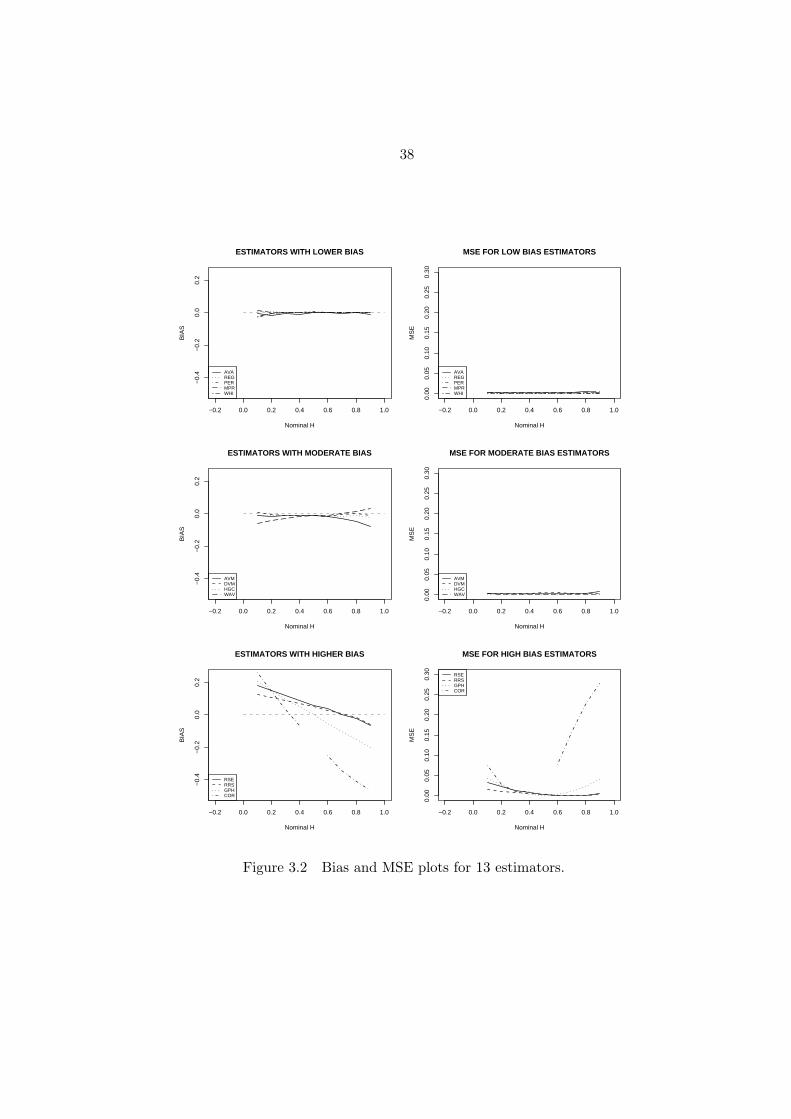
Tables 3.1 and 3.2, and Figure 3.2 present the statistical evaluation of the different
estimators via simulated fractional Brownian motion with H ∈ [0.1, 0.9]. For each es-
timation method described in Section 3.2.2 above and for each nominal value of H, we
calculate the estimators Hr for r = 1, ..., R = 100 replicates. Table 3.1 lists the means of
Hr, the standard deviations σ, and the root mean square error√MSE calculated over the
100 replications. Recall that the covariance relation estimator (COR) is only defined for
H 6= 12 .
Bias of the estimators can be inferred from Mean(Hr) − nominal H. The (simulated)
bias values are shown in Figure 3.2, left panel. From top to bottom, the left panel of Figure
3.2 includes estimators with lower, moderate, and higher bias. The right panel of Figure
3.2 shows the MSE for the three groups of estimators.
Two groups of estimators show the lowest bias: The “sophisticated” block-based esti-
mators AVA and REG, and the estimators PER, MPR and WHI that are based directly on
the periodogram. The R/S-based estimators RRS and RSE, the covariance relation estima-
tor COR, and the Geweke / Porter-Hudak estimator show the largest bias. For these five
estimators the bias results depend strongly on H, which is also the case for the moderate

36
−7 −6 −5 −4 −3 −2 −1
−10
−6
−2
log(frequency)
log(
perio
dogr
am)
Period Method, H=0.3
−7 −6 −5 −4 −3 −2−
7−
6−
5−
4−
3log(frequency)
log(
perio
dogr
am)
Modified Period Method, H=0.3
−7 −6 −5 −4 −3 −2 −1
−6
−4
−2
0
log(frequency)
log(
perio
dogr
am)
Period Method, H=0.5
−7 −6 −5 −4 −3 −2
−4
−2
0
log(frequency)
log(
perio
dogr
am)
Modified Period Method, H=0.5
−7 −6 −5 −4 −3 −2 −1
−8
−4
0
log(frequency)
log(
perio
dogr
am)
Period Method, H=0.7
−7 −6 −5 −4 −3 −2
−2
−1
01
log(frequency)
log(
perio
dogr
am)
Modified Period Method, H=0.7
Figure 3.1 Period method and modified period method for a certain fGn,
and H=0.3, 0.5, 0.7.

37
Table 3.1 Statistical assessment of estimators for H
Estimation Nominal HMethod 0.1 0.2 0.3 0.4 0.5 0.6 0.7 0.8 0.9
Mean (Hr)) 0.228 0.309 0.389 0.468 0.55 0.629 0.708 0.782 0.842RRS σ 0.008 0.01 0.011 0.013 0.015 0.016 0.015 0.019 0.017√
MSE 0.128 0.109 0.09 0.069 0.052 0.033 0.017 0.026 0.06
Mean (Hr) 0.279 0.347 0.417 0.49 0.56 0.638 0.705 0.776 0.831RSE σ 0.01 0.015 0.018 0.023 0.023 0.027 0.03 0.035 0.037√
MSE 0.179 0.148 0.119 0.093 0.065 0.046 0.03 0.042 0.078
Mean (Hr) 0.088 0.187 0.288 0.388 0.491 0.588 0.684 0.79 0.877HGC σ 0.016 0.023 0.029 0.041 0.038 0.039 0.051 0.063 0.055√
MSE 0.02 0.027 0.032 0.043 0.039 0.04 0.053 0.063 0.059
Mean (Hr) 0.037 0.161 0.273 0.381 0.486 0.591 0.702 0.813 0.933WAV σ 0.008 0.009 0.008 0.01 0.011 0.011 0.012 0.014 0.025√
MSE 0.063 0.04 0.028 0.021 0.018 0.015 0.012 0.019 0.041
Mean (Hr) 0.359 0.341 0.335 0.335 - 0.348 0.355 0.389 0.435COR σ 0.092 0.088 0.097 0.086 - 0.113 0.195 0.237 0.252√
MSE 0.275 0.166 0.103 0.107 - 0.276 0.396 0.474 0.527
Mean (Hr) 0.089 0.183 0.292 0.386 0.488 0.585 0.668 0.752 0.819AVM σ 0.05 0.054 0.054 0.056 0.049 0.045 0.047 0.044 0.046√
MSE 0.051 0.057 0.054 0.057 0.05 0.047 0.056 0.065 0.092
Mean (Hr) 0.107 0.193 0.292 0.387 0.488 0.584 0.694 0.8 0.886DVM σ 0.052 0.059 0.062 0.062 0.071 0.068 0.055 0.063 0.056√
MSE 0.053 0.059 0.062 0.063 0.071 0.07 0.055 0.063 0.058
Mean (Hr) 0.092 0.184 0.297 0.39 0.5 0.598 0.694 0.801 0.886AVA σ 0.056 0.058 0.057 0.057 0.051 0.046 0.054 0.065 0.053√
MSE 0.056 0.06 0.057 0.058 0.051 0.046 0.054 0.065 0.055
Mean (Hr) 0.109 0.206 0.303 0.403 0.502 0.599 0.7 0.8 0.898REG σ 0.006 0.011 0.013 0.019 0.021 0.024 0.021 0.03 0.028√
MSE 0.011 0.012 0.013 0.019 0.021 0.024 0.021 0.03 0.028
Mean (Hr) 0.069 0.192 0.299 0.4 0.505 0.602 0.698 0.801 0.901PER σ 0.03 0.031 0.027 0.033 0.033 0.029 0.028 0.028 0.031√
MSE 0.043 0.032 0.027 0.033 0.033 0.029 0.028 0.028 0.031
Mean (Hr) 0.111 0.202 0.298 0.401 0.5 0.601 0.702 0.8 0.898MPR σ 0.051 0.057 0.059 0.056 0.061 0.058 0.055 0.054 0.07√
MSE 0.051 0.057 0.059 0.056 0.06 0.058 0.055 0.054 0.07
Mean (Hr) 0.076 0.193 0.299 0.4 0.499 0.6 0.701 0.799 0.9WHI σ 0.006 0.005 0.005 0.006 0.006 0.006 0.006 0.007 0.007√
MSE 0.025 0.009 0.005 0.006 0.006 0.006 0.006 0.007 0.007
Mean (Hr) 0.305 0.352 0.397 0.449 0.5 0.548 0.6 0.65 0.701GPH σ 0.035 0.037 0.034 0.036 0.035 0.034 0.034 0.034 0.039√
MSE 0.208 0.157 0.103 0.061 0.035 0.062 0.106 0.154 0.202
38
−0.2 0.0 0.2 0.4 0.6 0.8 1.0
−0.
4−
0.2
0.0
0.2
Nominal H
BIA
S
ESTIMATORS WITH LOWER BIAS
AVAREGPERMPRWHI
−0.2 0.0 0.2 0.4 0.6 0.8 1.0
0.00
0.05
0.10
0.15
0.20
0.25
0.30
Nominal H
MS
E
MSE FOR LOW BIAS ESTIMATORS
AVAREGPERMPRWHI
−0.2 0.0 0.2 0.4 0.6 0.8 1.0
−0.
4−
0.2
0.0
0.2
Nominal H
BIA
S
ESTIMATORS WITH MODERATE BIAS
AVMDVMHGCWAV
−0.2 0.0 0.2 0.4 0.6 0.8 1.0
0.00
0.05
0.10
0.15
0.20
0.25
0.30
Nominal H
MS
E
MSE FOR MODERATE BIAS ESTIMATORS
AVMDVMHGCWAV
−0.2 0.0 0.2 0.4 0.6 0.8 1.0
−0.
4−
0.2
0.0
0.2
Nominal H
BIA
S
ESTIMATORS WITH HIGHER BIAS
RSERRSGPHCOR
−0.2 0.0 0.2 0.4 0.6 0.8 1.0
0.00
0.05
0.10
0.15
0.20
0.25
0.30
Nominal H
MS
E
MSE FOR HIGH BIAS ESTIMATORS
RSERRSGPHCOR
Figure 3.2 Bias and MSE plots for 13 estimators.

39
Table 3.2 Number of estimates of H outside of the (0, 1) range for each
nominal H value and each method that had at least one out-
-of-range event
Nominal H WAV COR AVM DVM AVA PER MPR
H=0.1 0 0 4 6 3 1 5
H=0.2 0 0 1 2 0 0 1
H=0.7 0 7 0 0 0 0 0
H=0.8 0 44 0 0 0 0 0
H=0.9 1 64 0 3 1 0 1
Total 1 115 5 11 4 1 7
bias estimators AVM, DVM, HGC and WAV. Because of their uneven bias for different
H−values, one has to interpret carefully any results that are obtained for time series with
time-varying H using these estimators, as we discuss in Section 3.3. In the group of low
bias estimators, the residuals of regression method (REG) and the periodogram method
(PER) show consistently low mean square error. So does the Whittle estimator (WHI).
We also note that the R/S-based estimators RRS and RSE exhibit larger MSE that is also
strongly H−dependent. The wavelet estimator (WAV) shows moderate bias and moderate
MSE, both of them depend strongly on the value of H. This estimator performs well for
H ∈ [0.5, 0.8], but part of the apparent good performance may be due to the larger length
of the simulated data series used for WAV.
Table 3.2 shows the number of trajectories (out of R = 100) that resulted in an estimate
of H outside of the parameter space (0, 1). We list only those estimators and H−values
that actually resulted in out-of-range values. Of the five low bias estimators, AVA, PER,
and MPR show some out-of-range events for H = 0.1 and/or H = 0.9. This leaves the
residuals of regression method (REG) as the low bias, low MSE estimator with no out-
of-range events. This estimator will be used in Section 3.3 to analyze the S&P500 data
series.
40
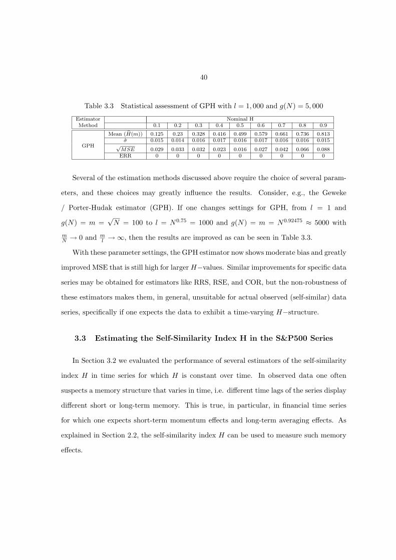
Table 3.3 Statistical assessment of GPH with l = 1, 000 and g(N) = 5, 000
Estimator Nominal HMethod 0.1 0.2 0.3 0.4 0.5 0.6 0.7 0.8 0.9
Mean (H(m)) 0.125 0.23 0.328 0.416 0.499 0.579 0.661 0.736 0.813σ 0.015 0.014 0.016 0.017 0.016 0.017 0.016 0.016 0.015
GPH √MSE 0.029 0.033 0.032 0.023 0.016 0.027 0.042 0.066 0.088ERR 0 0 0 0 0 0 0 0 0
Several of the estimation methods discussed above require the choice of several param-
eters, and these choices may greatly influence the results. Consider, e.g., the Geweke
/ Porter-Hudak estimator (GPH). If one changes settings for GPH, from l = 1 and
g(N) = m =√N = 100 to l = N0.75 = 1000 and g(N) = m = N0.92475 ≈ 5000 with
mN → 0 and m
l → ∞, then the results are improved as can be seen in Table 3.3.
With these parameter settings, the GPH estimator now shows moderate bias and greatly
improved MSE that is still high for largerH−values. Similar improvements for specific data
series may be obtained for estimators like RRS, RSE, and COR, but the non-robustness of
these estimators makes them, in general, unsuitable for actual observed (self-similar) data
series, specifically if one expects the data to exhibit a time-varying H−structure.
3.3 Estimating the Self-Similarity Index H in the S&P500 Series
In Section 3.2 we evaluated the performance of several estimators of the self-similarity
index H in time series for which H is constant over time. In observed data one often
suspects a memory structure that varies in time, i.e. different time lags of the series display
different short or long-term memory. This is true, in particular, in financial time series
for which one expects short-term momentum effects and long-term averaging effects. As
explained in Section 2.2, the self-similarity index H can be used to measure such memory
effects.

41
The Standard and Poor 500 (S&P500) series has been analyzed for its memory struc-
ture, notably by Peters (1996, for example, pages 47, 77, 83, 88, 112 and 113 as well as
Figures 7.6, 7.7, 8.1, 8.2, 8.3, 9.1 and 9.2) and by Bayraktar et al. (2004, Section 3, pp.
16-20). Peters bases his analysis on the R/S statistic and Bayraktar et al. on a wavelet
analysis. According to Section 3.2, the R/S method shows substantial bias (for fractional
Brownian motion) that also depends on the given value of H and may therefore mask the
actual memory structure in the S&P500 series.
In this section, we explore two issues that may impact inferences about the memory
structure in the S&P500 series:
• The effect of maximum block size used in the estimation of H when implementing
methods for estimating H that require blocking methods, and
• The effect of time on H, that is, whether the memory structure in the S&P500
changes over time.
The first of these two issues refers to a potential nuisance effect creeping into the
estimation process. Is it possible that different choices of maximum block size might lead
to different inferences about memory? The issue in the second bullet may be of greater
interest: If financial markets have different memory structures when looked at over different
periods then it might be possible to identify economic or other factors that are associated
with those structural memory changes.
At the end of this discussion in Section 3.3.4 we also study how to empirically test
hypotheses about the value of the underlying true H in a given series or in a subset of
a given series. To do so we revisit the scrambling method discussed by Peters (1996)
that permits testing whether estimates of H that differ from the null value of 0.5, can be

42
attributed to memory structure in the series (or in the subset of the series) or are due to
noise in the estimate resulting from, for example, inadequate data.
In exploring the different effects of time on the estimation of H we first consider simu-
lated fGn sequences and then we analyze the S&P500 data series so that we can compare
results. In both cases, we implement the residuals of regression method (REG) and the
method due to Whittle (WHI) that showed low bias and mean square error in our simula-
tions in Section 3.2. For comparison with the literature we also show results for the R/S
statistic. We now introduce notation that will be used in the remainder of this section.
Denote by Pk, k = 1, ..., N the observed weekly closing values of the S&P500 index
series between Jan. 3, 1950 and Nov. 27, 2006. To account for the compounding effect of
financial data, we consider the time series Qk := log(
Pk
P1
), k = 1, ..., N. But the series
Qk cannot be self-similar unless we expect E(Pk) = E(P1) for all k. It is therefore typical
to focus on the log of returns
Sk := log
(Pk
Pk−1
)
for k = 2, ..., N to assess memory structures based on self-similarity within the S&P500
time series, i.e. we assume that Sk, k = 1, ..., N follows a self-similar process with
stationary increments, which we denote Xk, k = 1, ..., N.
We can explore the S&P500 series at different levels of resolution. These include (but
are not limited to) daily, weekly and monthly observations, which correspond to the value
of the index at closing of each time period. Regardless of the data we use for analysis, we
can obtain estimates of H using the different methods described in the previous section.
Here, we focus on the estimators RSS, RSE and REG, all of which require that we divide
the series into a sequence of non-overlapping blocks as described below, and on the Whittle
estimator (WHI), which does not require blocking. We describe the approaches using the
example of weekly data.

43
Let Xk, k = 1, ..., N be a given time series (e.g., a series of increments) with values
in R, and denote by 0 < L1 < L2 < ... < LU a sequence of maximum block sizes where
Lu = L1 + (u − 1) · step. For weekly data, we choose L1 = 48, step = 4 weeks and
consequently, LU = 960 for U = 228.
To implement the REG and the RRS methods for estimating H, given a maximum
block size L∗, we divide the observed series into a sequence of non-overlapping blocks of
sizes nj+1 = nmin + j; j = 0, 1, ...L∗ − nmin. We chose nmin = 24. For any given block
size nj < L∗, the number of blocks into which we divide the data is therefore given by
bj = N/nj . To compute an estimator H(L∗) we proceed as follows:
1. In each non-overlapping block of size nj we obtain the statistic η(nj , L∗), which we
will use to compute the estimator H(L∗) according to one of the estimation methods
presented in Section 3.2.2. Thus, for a block size equal to nj , we obtain bj values of
the statistic.
2. Averaging these bj values results in a statistic denoted by η(nj , L∗). We obtain
L∗ − nmin + 1 such averages for each L∗.
3. The estimator H(L∗) of the self-similarity index is computed from the averages
η(nj , L∗) according to one of the methods outlined in Section 3.2.2. For example,
in the case of the RRS method, the averages η correspond to averages of the R/S
statistic and to obtain H(L∗) we regress those η(nj , L∗) on the log of nj ≤ L∗.
In the case of the WHI estimator, blocks of size Lu are constructed but no further
blocking is required. The series is then divided into blocks of size Lu, u = 1, ..., U to obtain
bu = N/Lu blocks. The WHI estimator is computed using observations in each block. For
a given maximum block size L∗, H(L∗) is obtained as the average, over the bu blocks, of

44
each of the block-level WHI estimators. Note that repeating this procedure for several
maximum block sizes L1, L2, ..., LU leads to an assessment of the effect of maximum block
size on the estimator H(Lu) (as stated in the first bullet above). We carried out the
procedure described above for weekly S&P500 observations and results are presented in
Section 3.3.1 below.
For a given maximum block size, the potential time-varying nature of the memory index
(estimated as the function H(Lu)) can be investigated by dividing the series into segments
and then obtaining the estimator of H separately in each segment. The segments can
be non-overlapping or can be constructed using a moving-window type of approach. For
example, for the S&P500 series we could divide the period Jan 3., 1950 - Nov. 27, 2006
into a set of overlapping time periods (e.g., from 1950 to 1960, 1952 to 1962, etc.) and
then obtain an estimate of H using data from each of the segments exclusively. In that
way, we can investigate whether inferences about the memory structure in the S&P500
depend on the time span under study. We carried out an analysis of this type and results
are presented in Section 3.3.2.
3.3.1 The effect of maximum block size on the estimate of H for fractional
Gaussian noise and for S&P500 returns for the time period Jan. 3, 1950
- Nov. 27, 2006
Several of the estimators of H that have been proposed in the literature require that
the data first be divided into non-overlapping blocks of appropriate size. For example,
the RRS, RSE and REG approaches rely on blocking (or windowing) approach. Since the
number of blocks and the maximum block size are, to a large extent, arbitrary, the question
arises as to whether the choice of maximum block size (and consequently, of number of
blocks) affects the value of the estimate of H computed from the data.

45
We first implemented the REG, RRS and WHI methods for estimating H on R = 10
simulated fGn sequences of length N = 10, 000 with nominal H values equal to 0.2, 0.4,
0.5, 0.6 and 0.8. (We ignore RSE, since it requires less assumptions and behaves worse
than the other three estimators.) As described earlier, maximum block sizes were fixed
at Lu = L1 + (u − 1) · step, where L1 = 48 and step = 4 weeks. The minimum block
size in every case was 24. Thus, for L1 = 48, the possible block sizes were 24, 25, ..., 48.
Figures 3.3 (a)-(e) show results. In the figures, we plot, for each of the three estimation
methods, the mean (over the R replicates) estimate of H for each maximum block size L,
as well as the ± one standard deviation bands for H (where the standard deviations are
also computed over the R replicates).
We note that in the case of fGn sequences, the estimate of H is essentially independent
of maximum block size and that this holds for any of the three estimation methods.
To explore whether the choice of maximum block size L affects the estimate of H
computed from weekly S&P500 observations,we proceeded in a similar way. For weekly
data (closing index values at the end of each week of Jan. 3, 1950 - Nov. 27, 2006), we
choose the same sequence of maximum block sizes L = 48, 52, ..., 960 that was used to
explore the fGn sequences and that for the S&500 series cover about 20 years in 4 week
intervals. We then proceeded with the estimation of H using a subset of the methods
described in Section 3.2.2. The results of the computations are shown in Figure 3.4, where
we depict H(L) for each of the four estimators obtained from the weekly time series.
As expected, the estimated H(L) values for the R/S based estimators RRS and RSE are
considerably larger than the values obtained via REG or via WHI, most likely a consequence
of the systematic positive bias of these two methods that we found in Section 3.2.3. Indeed,
the H−dependent bias of the RSE estimator results in a HRSE(L) curve that shows little
structure for weekly data. The residuals of regression method (REG) shows some roughness

46
0 200 400 600 800 1000
0.2
0.6
Maximum Block Size
H(a)
REGRRS
WHI
0 200 400 600 800 1000
0.2
0.6
Maximum Block Size
H
(b)
REGRRS
WHI
0 200 400 600 800 1000
0.2
0.6
Maximum Block Size
H
(c)
REGRRS
WHI
0 200 400 600 800 1000
0.2
0.6
Maximum Block Size
H
(d)
REGRRS
WHI
0 200 400 600 800 1000
0.2
0.6
Maximum Block Size
H
(e)
REGRRS
WHI
Figure 3.3 Estimate H and one-standard deviation confidence bands as
a function of maximum block size L and using three different
estimation methods. From (a) to (e) the fGn sequences had
nominalH values equal to 0.2, 0.4, 0.5, 0.6 and 0.8, respectively.

47
0 200 400 600 800 1000
0.3
0.4
0.5
0.6
0.7
Maximum Block Size (in WEEKS)
H
Weekly price data, 48−960 Ws every 4
REGRSE
RRSWHI
Figure 3.4 H as a function of time lag.

48
for the weekly data graphs for small window sizes.
For the REG estimator, we obtain the following results for S&P500 weekly returns over
the time period Jan. 3, 1950 to Nov. 27, 2006:
• The estimated memory parameter H(L) increases from about H(48) = 0.47 to
H(236) = 0.55 and then decreases to H(960) = 0.43.
• Within the interval of increase [48, 236] and the interval of decrease [236, 960] the
behavior of H(L) is basically monotone.
• The curve H(L) intersects the H = 0.5 line at maximum block sizes of 92 and of 480.
Hence the S&P500 data shows anti-persistent and mean-reverting behavior for blocks
of maximum size L ≤ 24 months and L ≥ 120 months, while for maximum block sizes
L ∈ [24, 120] months the series shows persistent and long-term effects, with a maximum at
about 80 months. The daily and monthly data (not shown) confirm these results.
Comparing these findings to the ones obtained in the literature by Peters (1996) we
notice, on the one hand, that the estimates obtained here result in substantially lower values
for H that the ones reported by Peters in Figure 9.1 for daily data. The main reason for
this difference might be the overestimation of H that results from using the R/S statistic.
Another reason could be that the time period used by Peters is 1928-1990 (for daily data),
while our analysis is based on the period 1950-2006, compare also the discussion in Section
3.3.2 below about the change of H over the years. The systematic overestimation of H
obtained when using the R/S statistic calls into question the relationship to the Pareto
distribution discussed by Peters on pp. 107-112. On the other hand, our analysis confirms
the observation that there is a specific maximum block size for which the long-range memory
parameter H achieves its maximum. We estimate this maximum block size to be L = 236

49
trading weeks (or about 58 months), as compared to Peters’ estimate of 1, 000 trading
days, or roughly 50 months (see Peters, 1996, Figures 8.2 and 9.1).
One other finding arises from the very different behavior of the estimators of H when
applied to the simulated fGn sequences and the real S&P500 data. We note that for fGn
sequences, the effect of maximum block size on H for any method is negligible for any of
the estimators used here. This is not true, however, in the case of the actual S&P500 data,
were we observe a pronounced effect of L on H except in the case of the empirical R/S
estimator and the Whittle estimator. This seems to suggest that the S&P500 sequence
does not behave like a fractional Gaussian noise sequence.
3.3.2 Time varying memory structure of S&P500 returns for time segments
during the period Jan. 3, 1950 - Nov. 27, 2006
The previous section discussed the effect of the choice of maximum block size on the
estimate of the memory parameter in fGn simulated sequences and in the S&P500 returns
over the entire period Jan. 3, 1950 - Nov. 27, 2006. Of potentially greater interest is the
question whether the memory structure of a time series changes over time. If financial
markets have different memory structures when looked at over different periods then it
might be possible to identify economic or other factors that are associated with those
structural memory changes.
Using daily log−returns for the period Jan. 2, 1928 - July 5, 1990 Peters found (via the
R/S estimator) that the memory parameter H was constant over these decades (Peters,
1996, pp. 113). Bayraktar et al. (2004) analyzed the period Jan. 1989 - May 2000
using a wavelet estimator for the time series given by the log−prices, i.e. they considered
Yk := log(
Pk
P1
). Their findings include a drop in HWAV around 1997 to a level close to 0.5.
Similar to our approach in Section 3.3.1, we first simulated fGn sequences for different

50
values of H and estimated the memory parameter in different time segments using the
estimators REG, RRS, and WHI. (We ignore RSE, since it requires less assumptions and
behaves worse than the other three estimators.) None of the three methods showed any
time-dependence of the index H in fGn sequences.
Using the REG estimator, we studied the segment-dependent memory structure of
S&P500 returns, based on weekly closing data for the time period Jan. 3, 1950 - Nov. 27,
2006. Figure 3.5 shows the time development of HREG(L) for blocks of maximum length (a)
L = 139 weeks (about 32 months), (b) L = 236 (about 54 months), and (c) L = 332 (about
77 months). These maximum block sizes were chosen to reflect the maximal estimated
H−value (HREG = 0.55 at L = 236) and the crossings of the HREG = 0.53 level (L = 139
and L = 332). For each maximum block size the figure shows the estimates HREG(L),
the linear regression line and a non-parametric regression line using local polynomials with
optimal bandwidth which is implemented as function “locpoly” in the statistical software
package R (e.g., Wand and Jones, 1995).
All three graphs show a linear negative trend over time for HREG(L). The non-
parametric regressions also suggest negative trends for all three block sizes, with short
time periods of increasing H in the 1950’s and 2000’s for the shortest window size L = 139.
In order to interpret these trends and to put the estimates for the time behavior of the
self-similarity index H of S&P500 logarithmic returns in context, we take a closer look at
Figure 3.5 (b), the variation of HREG over time for block size L = 236 (about 54 months,
or 4.5 years). For each time segment i = 1, ..., 12 the value HREG(i) estimates H over the
previous period of 236 trading weeks, e.g. H(6)REG(L = 236) estimates H for the period July
1972 - Jan. 1977 and H(12)REG(L = 236) estimates H for the period July 1999 - Jan. 2004.
According to the monotonicity intervals of Figure 3.5 (b), one can aggregate the 12 time
segments into seven segments, as shown in Table 3.4. To account for the block size, we list

510.
00.
40.
8
(a)
Date of Segments(i)
H(i)
BandWidth= 1.555
May 1963 Sep. 1976 Jan. 1990 May 2003
0.0
0.4
0.8
(b)
Date of Segments(i)
H(i)
BandWidth= 1.853
Jan. 1959 Jan. 1968 Jan. 1977 Jan. 1986 Jan. 1995 Jan. 2004
0.0
0.4
0.8
(c)
Date of Segments(i)
H(i)
BandWidth= 0.725
Jun. 1956 Nov. 1962 Apr. 1969 Sep. 1975 Feb. 1982 Jul. 1988 Dec. 1994 May 2001
Figure 3.5 H over time for three different maximum block sizes.

52
Table 3.4 Monotonicity intervals of H for maximum block size 4.5 years
Interval Period Length H tendency
1 1/50-10/56 6y 9m ↑2 10/56-4/61 4y 6m ↓3 4/61-10/74 13y 6m ↑4 10/74-4/79 4y 6m ↓5 4/79-10/83 4y 6m ↑6 10/83-4/97 13y 6m ↓7 4/97-1/2004 6y 9m ↑
the intervals with breaks at 1/2 the maximum block size, i.e. at 2 years and 3 months.
A decrease of H during period i indicates stronger short term memory dependence
within this period, i.e. the time series shows less persistence and a stronger mean-reverting
tendency. It appears that the memory index H of the S&P500 weekly data has shown
values below 0.5 since around 1982, meaning that the market has been dominated for this
time period by increasingly short memory effects. This trend may have been reversed
during the last few years, at least for shorter block sizes.
3.3.3 The combined effect of maximum block size and decade on the estimated
value of H
We now investigate the combined effect of choice of maximum block size and time
segment on the estimated H. As we did earlier, we first focus on the estimates computed
from simulated fGn sequences and then explore the results obtained from the S&P500
series.
To investigate the combined effect of maximum block size and time segment we pro-
ceeded as follows for the simulated fGn sequences:
1. We considered moving time segments of size 500 observations.

53
2. For a 100-observation step, each segment had an overlap of 400 observations with the
preceding segment.
3. Within each segment, we computed H(Lu), for Lu = 50, 55, ..., 250 observations.
That is, we considered b = 250 − 50 + 1 = 201 possible maximum block sizes.
In the case of the observed S&P500 series, the process was similar except that the
moving window segments were of length 10 years and the moving step was two years.
Further, for the S&P500, Lu = 48, 52, 56, ..., 240 for a total of b = 193 possible values of L.
Figure 3.6 (a)-(e) correspond to results obtained from the fGn simulated sequences with
nominal H values of 0.2, 0.4, 0.5, 0.6 and 0.8. Figure 3.7 (a) and (b) correspond to results
obtained from the S&P500 series.
In Figure 3.6 (a)-(e) and in the (a) panel of Figure 3.7 we present the maximum (over
the b maximum block sizes) value of H(Lu) in each time segment. The (b) panel in Figure
3.7 shows the maximum block size Lu within each time segment at which the highest value
of H(Lu) was obtained. As before, we see that for fGn sequences, the effect of maximum
block size is negligible for all estimation methods and all nominal H values. (Clearly, we do
not expect to see a time segment effect in the simulated series.) In the case of the S&P500,
however, we observe that the maximum value of H(Lu) varies between a low of about 0.4
and a high of about 0.6 (for the Whittle estimator) and that the maximum block sizes that
produce those maximal estimates are also highly variable.
Panel (a) of Figure 3.7 is consistent with the results discussed in Section 3.3.2. The
variability in panel (b) of this figure calls into question the significance of the block size
when analyzing memory structures in the S&P500 return data: None of the three estimators
shows a consistent block size over the time period from 1950 - 2006, indicating that the
observations in Section 3.3.1 refer to averages over time segments within this period. In
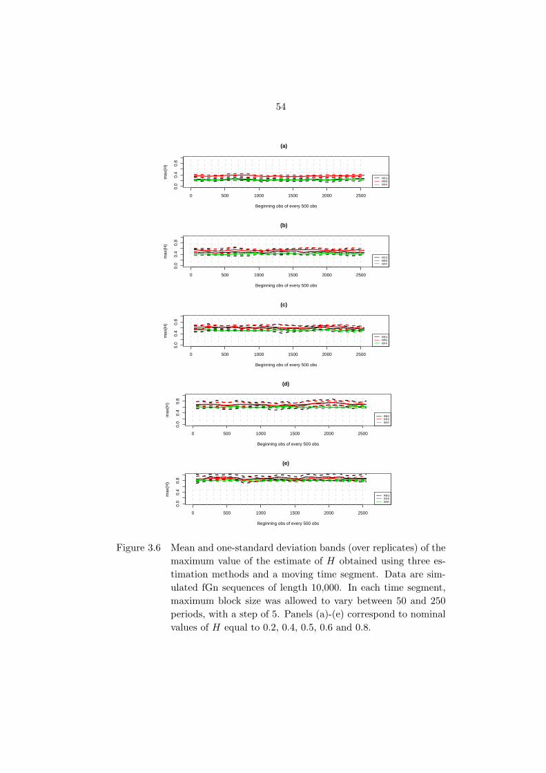
54
0 500 1000 1500 2000 2500
0.0
0.4
0.8
Beginning obs of every 500 obs
max
(H)
(a)
REGRRSWHI
0 500 1000 1500 2000 2500
0.0
0.4
0.8
Beginning obs of every 500 obs
max
(H)
(b)
REGRRSWHI
0 500 1000 1500 2000 2500
0.0
0.4
0.8
Beginning obs of every 500 obs
max
(H)
(c)
REGRRSWHI
0 500 1000 1500 2000 2500
0.0
0.4
0.8
Beginning obs of every 500 obs
max
(H)
(d)
REGRRSWHI
0 500 1000 1500 2000 2500
0.0
0.4
0.8
Beginning obs of every 500 obs
max
(H)
(e)
REGRRSWHI
Figure 3.6 Mean and one-standard deviation bands (over replicates) of the
maximum value of the estimate of H obtained using three es-
timation methods and a moving time segment. Data are sim-
ulated fGn sequences of length 10,000. In each time segment,
maximum block size was allowed to vary between 50 and 250
periods, with a step of 5. Panels (a)-(e) correspond to nominal
values of H equal to 0.2, 0.4, 0.5, 0.6 and 0.8.
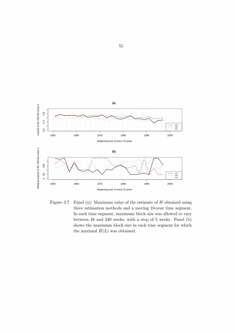
55
1950 1960 1970 1980 1990 2000
0.0
0.4
0.8
Beginning year of every 10 years
max
(H)
of 4
8−24
0 W
s ev
ery
4
(a)
REG
RRS
WHI
1950 1960 1970 1980 1990 2000
050
150
Beginning year of every 10 years
Wee
k at
max
(H)
of 4
8−24
0 W
s ev
ery
4
(b)
REG
RRS
WHI
Figure 3.7 Panel (a): Maximum value of the estimate of H obtained using
three estimation methods and a moving 10-year time segment.
In each time segment, maximum block size was allowed to vary
between 48 and 240 weeks, with a step of 5 weeks. Panel (b)
shows the maximum block size in each time segment for which
the maximal H(L) was obtained.

56
particular, interpretations of notable memory effects in the S&P500 time series based on
maximal block sizes (compare, e.g. Peters, 1996) have to be taken with some care, at least
for the second half of the 20th century.
3.3.4 Validation of the estimation of the self-similarity index
Regardless of the method that is used to obtain an estimate H(L), it is often of interest
to test hypotheses about the underlying, unobservable H. One hypothesis of interest is
whether H = 0.5 or in other words, whether the series on which the estimate H is based has
no memory structure. In principle, to carry out a test of the null hypothesis H0 : H = 0.5
against the alternative Ha : H 6= 0.5 we need to derive the distribution of H(L) under the
null hypothesis.
An alternative approach consists in approximating the distribution using an empiri-
cal non-parametric approach. The resulting test is similar to the usual permutation test
originally proposed by Pitman (1938, pp. 323-324) and more recently discussed by, e.g.,
Welch (1990, Section 2). In the context of an empirical non-parametric test, Scheinkman
and LeBaron (1989, pp. 317-318) proposed a test called the scrambling test to investigate
whether a series has the property of long memory.
The idea behind the scrambling test is the following: If a series exhibits long memory,
then the residuals of the regression of the current observation on the previous observation
would be correlated. Suppose now that the observation at time k is substituted by the value
obtained by adding a randomly chosen estimated regression residual to the observation at
time k − 1. The new sequence is called a scrambled sequence and in principle would have
less of a memory structure than the original sequence. The test therefore proceeds as
follows:
1. Obtain the estimated residuals from the regression of Yk on Yk−1, k = 2, ..., N .

57
2. Using the observed Y1 as the “anchor”, construct a scrambled series of length N by
replacing Y2, ..., YN by values obtained as the sum of the previous value and a residual
randomly chosen from among the N residuals computed in Step 1.
3. Repeat the second step M times to obtain M scrambled series.
We then obtain M+1 estimates of H, one from the original series and one from each of
the M scrambled series, which we denote H(L) and H(i)(L), i = 1, ...,M , respectively. The
empirical distribution of the H(i)(L) can be viewed as the distribution of the estimator un-
der the null hypothesis (i.e. under the random walk hypothesis for H∗ = 12), although this
is not strictly the case since only residuals and not observations themselves are permuted.
This pseudo-null distribution nonetheless provides a reference against which to compare
H(L). If H(L) is likely under the pseudo-null distribution, then this suggests that the
original series does not exhibit a memory structure.
In order to test the validity of our estimates of the memory parameter H we imple-
mented the scrambling test as described in above. To illustrate the procedure, we first
consider three simulated fractional Brownian motion sequences of length 10, 000 with dif-
ferent H−values H = 0.3, 0.5, and 0.7. For each of the original sequences we implemented
the regression method to obtain an estimate HREG of H, which in all cases was close to
the nominal value. We then scrambled each sequence M = 100 times and re-estimated H
in each of the scrambled sequences. Figure 3.8 shows, for each nominal value of H, the
histogram of the estimates computed from each of the scrambled sequences. The vertical
bar on each of the plots indicates the value of HREG obtained from each of the three un-
scrambled series. From the figure we see that for small or large values of H, the estimate
HREG is very unlikely under the random walk assumption. In both cases we would tend to
conclude that the original sequence had short (for H = 0.3) or long (for H = 0.7) memory.
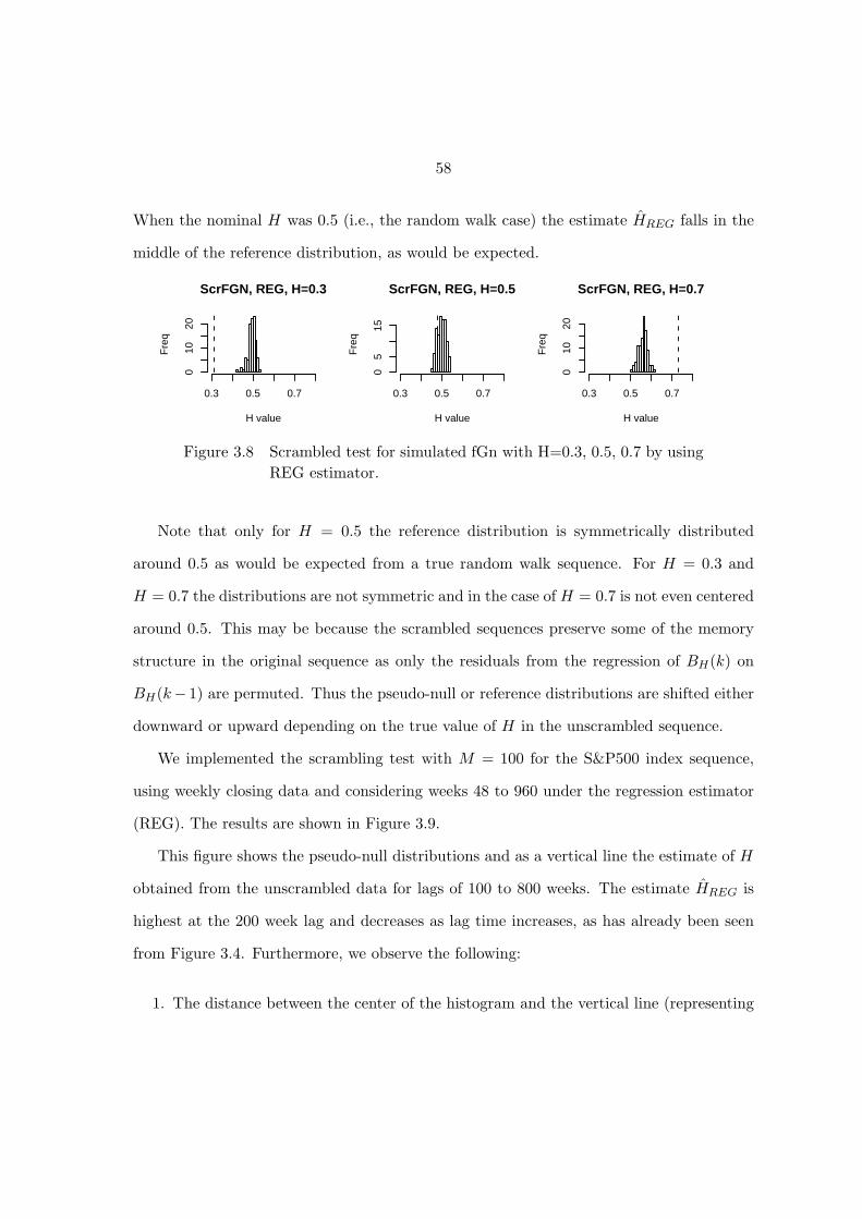
58
When the nominal H was 0.5 (i.e., the random walk case) the estimate HREG falls in the
middle of the reference distribution, as would be expected.
ScrFGN, REG, H=0.3
H value
Fre
q
0.3 0.5 0.7
010
20
ScrFGN, REG, H=0.5
H value
Fre
q
0.3 0.5 0.7
05
15
ScrFGN, REG, H=0.7
H value
Fre
q
0.3 0.5 0.7
010
20
Figure 3.8 Scrambled test for simulated fGn with H=0.3, 0.5, 0.7 by using
REG estimator.
Note that only for H = 0.5 the reference distribution is symmetrically distributed
around 0.5 as would be expected from a true random walk sequence. For H = 0.3 and
H = 0.7 the distributions are not symmetric and in the case of H = 0.7 is not even centered
around 0.5. This may be because the scrambled sequences preserve some of the memory
structure in the original sequence as only the residuals from the regression of BH(k) on
BH(k− 1) are permuted. Thus the pseudo-null or reference distributions are shifted either
downward or upward depending on the true value of H in the unscrambled sequence.
We implemented the scrambling test with M = 100 for the S&P500 index sequence,
using weekly closing data and considering weeks 48 to 960 under the regression estimator
(REG). The results are shown in Figure 3.9.
This figure shows the pseudo-null distributions and as a vertical line the estimate of H
obtained from the unscrambled data for lags of 100 to 800 weeks. The estimate HREG is
highest at the 200 week lag and decreases as lag time increases, as has already been seen
from Figure 3.4. Furthermore, we observe the following:
1. The distance between the center of the histogram and the vertical line (representing

59
100W
H value
Fre
q
0.30 0.35 0.40 0.45 0.50 0.55 0.60
020
40
200W
H valueF
req
0.30 0.35 0.40 0.45 0.50 0.55 0.60
020
40
300W
H value
Fre
q
0.30 0.35 0.40 0.45 0.50 0.55 0.60
020
40
400W
H value
Fre
q
0.30 0.35 0.40 0.45 0.50 0.55 0.60
020
40
600W
H value
Fre
q
0.30 0.35 0.40 0.45 0.50 0.55 0.60
020
40
800W
H value
Fre
q
0.30 0.35 0.40 0.45 0.50 0.55 0.60
020
40
Figure 3.9 Histograms of REG estimations for unscrambled and scrambled
weekly data.

60
the unscrambled data) decreases, as the block size grows from 100 weeks to 800 weeks.
This means that the estimated value of H becomes less dependent on the order of
the observations as the block size grows.
2. For intermediate block sizes, i.e. when the estimator HREG of the original, unscram-
bled data series is above 0.53, the center of the histogram is closer to 0.5 than the
vertical line, i.e. the value of HREG for the unscrambled data. This indicates that
S&P500 index behaves like a long memory time series for blocks of size L ∈ [100, 350]
weeks.
3. For blocks of size L < 100 weeks and L > 350 weeks, the center of the histogram
is below 0.5, which would imply that the scrambled data has short memory. Thus
when the estimated H from the unscrambled data is around 0.5 the implemented
scrambling test fails. We comment on several reasons for this behavior below.
The main reason for the failure of the scrambling test in our context for maximum block
sizes L < 100 weeks and L > 350 weeks, seems to be the number of available observations
in the blocks. The maximum block size for weekly data includes 1000 observations that can
be used for the estimation of H, which may be insufficient for H < 0.53 as shown above
for fractional Brownian motion. Furthermore, the scrambled sequences preserve some of
the memory structure in the original sequence as only the residuals from the regression
of Sn on Sn−1 are permuted. Finally, the actual S&P500 log−return data series may not
satisfy the assumption on stationary increments that is implicit in the use of the regression
estimator (REG).

61
CHAPTER 4. FRACTIONAL STOCHASTIC MODELS
4.1 Introduction
In order to make these existing financial models capable to obtain a long or short
memory structure, a heuristic method is to incorporate fractional processes, e.g. fractional
Brownian motion, in them. Following this idea, our research deals with the stochastic
volatility models, extend the LogOU and CIR model (two of the popular existing finance
models), argued carefully about the support area of the fractional parameters that well
define the pathwise integral with respect to fBm, and explore the memory structures un-
derlying these two modified models through simulation and analytical approaches.
The chapter is organized as follows. We first revisit the Black-Scholes model and its
extensions (Section 4.2). We then summarize existing results on the Hurst exponent and
show that the current LogOU and CIR model fail to capture the memory structure in the
data (Section 4.3). In Section 4.4, we introduce fractional Brownian motion processes.
Later, in Section 4.5, we propose the modified LogOU stochastic volatility models, and
discuss the well-definedness of its solution in the pathwise sense. The joint behavior of
the price and volatility processes under the modified LogOU is also studied in this section.
The related simulations are conducted in Section 4.6. The well-definedness problem and
the joint behavior of the price and volatility of modified CIR models are explored similarly
in Section 4.7. Finally in Section 4.8 we propose future avenues for research.

62
4.2 Black-Scholes Model and its Extensions
Linear models that can be used to describe the evolution of prices and the variability
in the prices of financial instruments over time have been discussed extensively in the
literature (Hull, 2002). One of the earlier efforts to jointly model prices and volatility
was the work by Black and Scholes (1973) which is described below. The Black-Scholes
approach involved several assumptions that cannot be justified in the case of financial
time series and thus several more general versions of the Black-Scholes model have been
proposed recently. Below we first introduce the simple Black-Scholes pricing model. We
then formulate a general version of the linear stochastic volatility model and then describe
several special cases of the general linear model that have appeared in the literature.
We use St to denote the stock price at time t and let Yt = log(St). Both Yt and St
are described by a probability space (Ω,F, P ) with the usual properties. In the models we
discuss below, Yt is the response process. The more general models also involve a process
Vt, the volatility of prices at time t. Note that for the general model, the Vt process is a
Markov process, while Yt itself is not. Jointly, however, Vt and Yt form a two-dimension
Markov process.
4.2.1 The Black-Scholes model
Under the assumptions of European options the Black-Scholes model for Yt, depends
on a constant drift µ and a constant volatility σ:
dYt = µdt+ σdWt, (4.1)
where Wt is Brownian motion defined on the probability space, and t ∈ R+.

63
4.2.2 General stochastic volatility model
If the constant volatility assumption in the simple Black-Scholes model is relaxed then
a more general approach to model Yt is
σt = f(Vt),
dYt = µdt+ σtdWyt ,
dVt = (a+ bVt)dt+ c(Vt)γdW ν
t ,
dW νt = ρdW y
t +√
1 − ρ2dWt,
(4.2)
for µ, a, b, c, γ, ρ unknown constant over time, and for W yt and Wt independent Brow-
nian motion processes. The model above is general in that it lets both prices and their
volatility change over time and allows for the presence of a feedback mechanism between
Yt and Vt. Because the two random drivers of the Yt and Vt processes are correlated with
correlation coefficient ρ, volatility can affect price and vice versa. However, instead of the
correlation between Yt and Vt, the focus of the manuscript is on the memory structure of
the stochastic volatility models, we therefore set ρ = 0 in the general model form, and later
their extensions do not consider the correlated random drivers of the Yt and Vt processes.
4.2.3 Log Ornstein-Uhlenbeck (LogOU) model
The Log Ornstein-Uhlenbeck model (Uhlenbeck and Ornstein, 1930) is one stochastic
volatility model. Here, the two random drivers are assumed to be independent and the
dynamics of Vt allow for a constant drift:
σt = f(Vt) = eVt
dYt = µdt+ σtdWyt ,
dVt = (a+ bVt)dt+ cdW vt ,
(4.3)

64
for µ, a, b, c constant over time and for W yt and W v
t independent Brownian motion pro-
cesses.
Further, to have a stationary solution for the volatility equation, we set a = 0, b < 0
and c > 0, and then have Vt is normally distributed with expectation and covariance
E (Vt) = 0, Cov (Vs, Vt) = − c2
2beb|s−t|,
and the conditional distribution of Vt given Vs (t > s) is also a normal distribution with
expectation and variance
E (Vt|Vs) = Vseb(t−s), V ar (Vt|Vs) = − c
2
2b
(1 − eb(t−s)
),
and the conditional distribution of Vt given V0 = v0 is a normal with expectation v0ebt
and covariance Cov (Vt, Vs|V0 = v0) = − c2
2b
(eb(t−s) − eb(t+s)
). (When t → ∞, the limiting
distribution for Vt is a normal distribution with expectation 0 and variance − c2
2b .)
4.2.4 Cox-Ingersoll-Ross (CIR) model
The Cox-Ingersoll-Ross model (Cox et al., 1985a, 1985b) is another commonly used
stochastic volatility model in financial applications. The CIR model is similar to the
LogOU model except the function used to define the volatility:
σt = f(Vt) =√Vt
dYt = µdt+ σtdWyt ,
dVt = (a+ bVt)dt+ c√VtdW
vt ,
(4.4)
for µ, a, b, c constant over time and for W yt and W v
t independent Brownian motion
processes. In application, the CIR model is often written in a different form:

65
σt = f(Vt) =√Vt
dYt = µdt+ σtdWyt ,
dVt = κ(θ − Vt)dt+ σv
√VtdW
vt ,
(4.5)
where κ = −b, θ = a/κ and σv = c. Usually, we assume that κ > 0, θ > 0 and σv > 0.
(I.e., assume a > 0, b < 0 and c > 0 in the first expression of CIR model.) Under these
assumptions the Vt process is mean-reverting. Under the assumption that both κ, θ are
positive, Vt can be shown to be a non-central χ2 random variable with the expectation
equal to
E (Vt|V0 = v0) = θ + (v0 − θ) e−κt
and variance equal to
V ar (Vt|V0 = v0) =θσ2
v
2κ+σ2
v
κ(v0 − θ) e−κt +
σ2v
κ
(θ
2− v0
)e−2κt.
The limiting distribution of Vt is a Gamma distribution with expectation θ and variance
θσ2v
2κ (Cox et al., 1985a, 1985b).
4.3 Memory Structure and the Hurst Exponent
Peters (1996) used the Hurst exponent to study a real dataset – S&P 500 price data in
a special way. Using the notation introduced earlier, the response variable for his analysis
was the return – (Yt − Yt−1), for Yt = log(St) and St = the stock price at time t. Given
a maximum block size N Peters computed the value of the R/S statistic in the following
steps:
1. For a certain reasonable increment of time N0, N0 ≤ N , divide the data into several
non-overlapping blocks, with sample size in each block equal to N0.

66
2. Calculate the R/S statistic in each of the blocks.
3. Average the R/S values of the statistic over all the blocks.
After obtaining the averaged value of the statistic for all reasonable increments of time
N0, N0 ≤ N , a regression based on the relationship between the R/S statistic and H can
be used to estimate H for a given maximum block of size N . Further, Peters repeated
the process for other choices of time window size N . This allows people to investigate
the estimates of H corresponds to different maximum block sizes. Below, we followed
Peters (1996) and produced Figure 4.1 shows the estimated Hurst exponent for different
time window sizes computed from the S&P 500 daily returns from January 2nd, 1980 to
December 29th, 2000.
0 500 1000 1500 2000
0.3
0.5
0.7
DAYS
H
Hurst Exponent for Daily S&P500, 252−2268 Ds every 10
Figure 4.1 Hurst exponent estimates for different window sizes for daily
S&P 500 data.
In Figure 4.1, the values of the estimated Hurst exponent over time are not always
0.5, but increase from 0.5 at the very beginning, peak to a value above 0.5 sometime
around three years, and then decrease to be around 0.5 (after some time around 6 years).
This figure unveils the complicated memory structure underlying a process. Other studies
supportive that memory structure underlying a process can be different from a random walk
or a short memory process include the study of precipitation in a local area (Mandelbrot
and Wallis, 1968), and the study of nanoscale single-molecule biophysics experiments (Kou

67
and Xie, 2004). These studies motivated us to extend the LogOU and the CIR model into
more general form in order to account for a short or long memory in a process.
4.4 Stochastic Integrals and Fractional Brownian Motion
Definition 4.4.1 (Øksendal, 2004): Let H ∈ (0, 1) be a constant. The (1-parameter)
fractional Brownian motion (fBm) with Hurst parameter (the self-similar index of this
process) H is the Gaussian process BH(t) = BH(t, ω), t ∈ R, ω ∈ Ω, satisfying BH(0) =
E[BH(t)] = 0, for all t ∈ R, and E[BH(s)BH(t)] = 12|s|2H + |t|2H − |s − t|2H, for
all s, t ∈ R. Here E(·) denotes the expectation with respect to the probability law P for
BH(t)t∈R = BH(t, ω) : t ∈ R, ω ∈ Ω, where (Ω,F) is a measurable space.
For this Gaussian process, two types of stochastic integrals are defined by people and
used a lot. One is the pathwise or forward integral, the other is the Skorohod (Wick-Ito)
integral. To facilitate the simulation method for the stochastic integral with respect to a
fractional Brownian motion, we choose the former way to define stochastic integrals with
respect to fractional Brownian motions.
The pathwise integral is usually denoted by
T∫
0
φ(t, ω)d−WHt .
Given the integrand φ(t, ω) is caglad (left-continuous with right sided limits), this integral
is described by Riemann sums:
Let 0 = t0 < t1 < · · · < tN = T be a partition of [0, T ]. Put ∆tk = tk+1 − tk and define
T∫
0
φ(t, ω)d−WHt = lim
∆tk→0
N−1∑
k=0
φ(tk, ω)(WH
tk+1−WH
tk
),

68
if the limit exists (e.g. in probability). Using a classical integration theory, one can prove
that the pathwise integral exists if the p-variation of t→ φ(t, ω) is finite for all p > (1−H)−1
and a given value of H ∈ (0, 1). (Øksendal, 2004.)
Notice that some forms of stochastic integrals with respect to fractional Brownian
motions may not be able to define in the pathwise sense for all the H values on (0, 1).
Therefore, the support area of the H value for the well-defined pathwise integrals should
be carefully stated. Some sufficient conditions for the well-defined pathwise integrals are
provided in literature, for example, by using q-variation which definition is mentioned in
Øksendal (2003, Page 19). Since t → WHt has finite q-variation if and only if q ≥ 1
H , we
see that if H < 12 then this theory does not even include integrals like (Øksendal, 2004)
T∫
0
WHt d−WH
t .
In other words, the support area of the H value this specific integral is [0.5, 1).
4.5 Fractional Log Ornstein-Uhlenbeck (LogOU) Model
4.5.1 The well-definedness of the fractional LogOU model system
An extension to the Ornstein-Uhlenbeck model, is to have a fractional Brownian motion
in the volatility equation to capture the possible long-range memory in the data. In other
words, a fractional Ornstein-Uhlenbeck (volatility) model can be defined as:
dV Ht = bV H
t dt+ cdWHv
t ,
for b and c constant over time and WHv
t being a fBm with the index Hv ∈ (0, 1). The
way to define dWHv
t is to follow the pathwise explanation. Since now, c is constant, this
extended version of the Ornstein-Uhlenbeck (volatility) model is well defined automatically.
69
Further, the solution of the stochastic equation in above mentioned by Hu (2002) is in the
following form:
V Ht = ebtV H
0 + c
t∫
0
e(t−s)bdWHv
s .
Cheridito et al. (2003) discussed the behaviors of the fractional Ornstein-Uhlenbeck process
in a pathwise sense, and mentioned that a stationary solution to this model is
V Ht = c
t∫
−∞
eb(t−s)dWHv
s .
Further, they proved some interesting results for to this integral.
Proposition 4.5.1 (Proposition A.1, Cheridito et al., 2003.) LetWH
t
t∈R
be a fBm
with H ∈ (0, 1]. Let −∞ ≤ a < ∞, and λ > 0. Then, for almost all ω ∈ Ω, we have the
following:
1. For all t > a,t∫
a
eλsdWHs (ω)
exists as a Riemann-Stieltjes integral and is equal to
eλtWHt (ω) − eλaWH
t (ω) − λ
t∫
a
WHs (ω)eλsds.
2. The functiont∫
a
eλsdWHs (ω), t > a
is continuous in t.
3. Let H ∈ (0, 12) ∪ (1
2 , 1], λ > 0 and −∞ ≤ a < b ≤ c < d <∞. Then
E
b∫
a
eλudWHu
d∫
c
eλνdWHν
= H(2H − 1)
b∫
a
eλu(
d∫
c
eλν(ν − u)2H−2dν)du.

70
Theorem 4.5.2 (Theorem 2.3, Cheridito et al., 2003.) Let H ∈ (0, 12) ∪ (1
2 , 1], and N =
1, 2, · · · . Then, for fixed t ∈ R and s→ ∞,
Cov(V H
t , V Ht+s
)=
1
2c2
N∑
n=1
|b|−2n
2n−1∏
k=0
(2H − k)
s2H−2n +O(s2H−2N−2).
Theorem 4.5.3 (Remark 2.4, Cheridito et al., 2003.) For all t, s ∈ R and H ∈ (0, 1), the
autocovariance function (ACVF) of the solution from fractional Ornstein-Uhlenbeck model
can be expressed explicitly as:
Cov(V H
t , V Ht+s
)= c2
Γ(2H + 1) sin(πH)
2π
∞∫
−∞
eisx|x|1−2H
|b|2 + x2dx, (4.6)
for i =√−1 .
Below, we provide a theorem on the well-definedness of the whole fractional LogOU
dynamic model system which includes both the fractional OU model as the fractional
volatility and the price model in the fractional form.
Theorem 4.5.4 Define a fractional LogOU dynamic model system as
dY Ht = µdt+ eV
Ht dWHy
t , dV Ht = bV H
t dt+ cdWHv
t ,
where WHy
t and WHv
t are two independent fractional Brownian motions with their own
self-similarity index being Hy and Hv and with V ar(WHy
1
)= V ar
(WHy
1
)= 1, and b < 0,
c > 0. Then, this dynamic system is well defined for all pairs of (Hv, Hy) ∈ (0, 1) × (0, 1)
that satisfy Hv +Hy ≥ 1.
Proof. For the theorem, it is enough to show that the following integral
Y HT = Y H
0 + µT +
T∫
0
eVHt dWHy
t (4.7)

71
is well defined for all pairs of (Hv, Hy) ∈ (0, 1)× (0, 1) that satisfy Hv +Hy ≥ 1. It is then
equivalent to show thatT∫
0
eVHt dWHy
t
is well defined for all pairs of (Hv, Hy) ∈ (0, 1) × (0, 1) that satisfy Hv +Hy ≥ 1.
According to Øksendal (2003), the p-variation of a process Xt on a time interval [0, T ]
with p > 0 is defined as
Vp (Xt, 0, T, ω) = lim|Π|→0
∑
Π
∣∣Xtk+1(ω) −Xtk(ω)
∣∣p = lim|Π|→0
∑
Π
∣∣Xtk+1−Xtk
∣∣p ,
where Π is a partition on the time interval [0, T ].
Further, given ω offering the solution V Ht a continuous function of time t, V H
t would
be bounded on the time interval [0, T ]. We denote the lower and higher bound of V Ht as
V Htl> 0 and V H
th> 0. By the mean value theorem, we then have
eV H
tl Vp
(V H
t , 0, T, ω)≤ Vp
(eV
Ht , 0, T, ω
)≤ e
V Hth Vp
(V H
t , 0, T, ω).
Therefore, the feature of p-variation of eVHt which can be thought as a function of t, is
same as V Ht . (In other words, the p-variation of eV
Ht is finite or infinite, if and only if the
p-variation of V Ht is finite or infinite.)
Similarly, but using the mean value theorem for integration, we can have that the
feature of p-variation of e−btV Ht is same as WHv
t – the random driver of V Ht . since the
p-variation of WHv
t finite if and only if q ≥ 1Hv , we have a finite p-variation of e−btV H
t if
and only if p ≥ 1Hv .
Further, if p ≥ 1Hv ≥ 1, we can show that
72
Vp
(V H
t , 0, T, ω)
= lim|Π|→0
∑
Π
∣∣∣V Htk+1
− V Htk
∣∣∣p
= lim|Π|→0
∑
Π
∣∣∣(ebtk+1 − ebtk
)e−btk+1V H
tk+1+ ebtk(e−btk+1V H
tk+1− e−btkV H
tk)∣∣∣p
≤ a positive number ×(1 − ebT
)+ a positive number × Vp
(e−btV H
t , 0, T, ω)<∞.
Thereby, the support area of the equation (4.7) is determined by the well-definedness of
T∫
0
V Ht dWHy
t .
Following the p-variation condition for the well-definedness of the pathwise solution to
a stochastic integral of fBm, we need the p-variation of V Ht finite for all p > (1 −Hy)−1,
and since the p-variation of V Ht finite if p ≥ 1
Hv , we have
(1 −Hy)−1 ≥ 1
Hv⇔ Hv +Hy ≥ 1.
4.5.2 The joint behavior of Y Ht and V H
t
Next, we discuss the memory structures of the volatility process described by the frac-
tional OU equation and the corresponding price process.
Proposition 4.5.5 For well-defined fractional LogOU dynamic model system
dY Ht = µdt+ eV
Ht dWHy
t , dV Ht = bV H
t dt+ cdWHv
t ,
where WHy
t and WHv
t are two independent fractional Brownian motions with their own
self-similarity index being Hy and Hv and with V ar(WHy
1
)= V ar
(WHy
1
)= 1, and b < 0,
c > 0,

73
1. V Ht has a short time memory if 0 < Hv ≤ 0.5 and shows a long time memory if
0.5 < Hv < 1. (The incremental process of V Ht always has a short time memory.)
2. the memory structure of ∆Y Ht := µ∆ + eV
Ht ∆WHy
t = µ∆ + eVHt
(WHy
t+1 −WHy
t
)
depends on Hy, i.e. a short time memory, a long time memory or no memory for
0 < Hy < 0.5, 0.5 < Hy < 1 or Hy = 0.5 respectively,
Proof.
1. For V Ht process
• if Hv = 0.5,∞∑
s=1
|Cov(V Ht , V H
t+s)| = − c2
2b
∞∑
s=1
e2bs <∞.
• if 0 < Hv < 0.5, by Theorem 4.5.2 (Theorem 2.3, Cheridito et al., 2003), there
exists a η > 0 such that
0 ≤∞∑
s=1
|Cov(V Ht , V H
t+s)|
≤ 1
2c2
∞∑
s=1
N∑
n=1
|b|−2n
∣∣∣∣∣2n−1∏
k=0
(2Hv − k)
∣∣∣∣∣ s2Hv−2n + a finite term
≤ 1
2c2
N∑
n=1
|b|−2n
∣∣∣∣∣2n−1∏
k=0
(2Hv − k)
∣∣∣∣∣∞∑
s=1
s−(1+η) + a finite term <∞.
• if 0.5 < Hv < 1, by Theorem 4.5.2 (Theorem 2.3, Cheridito et al., 2003),
∞∑
s=1
|Cov(V Ht , V H
t+s)| ≥1
2c2
∞∑
s=1
|b|−2 |2Hv(2Hv − 1)| s2H−2 + a finite term = ∞.

74
As to the incremental process of V Ht , we use δ for time lag and define ⌈δ⌉ as the
smallest integer greater than δ. Then, we have
∞∑
s=1
|Cov(∆V Ht ,∆V H
t+s)|
=∞∑
s=⌈δ⌉+1
[1
2c2
N∑
n=1
|b|−2n
∣∣∣∣∣2n−1∏
k=0
(2Hv − k)
∣∣∣∣∣∣∣2s2Hv−2n − (s+ δ)2Hv−2n
− (s− δ)2Hv−2n∣∣]+ a finite term
=1
2c2
N∑
n=1
|b|−2n
∣∣∣∣∣2n−1∏
k=0
(2Hv − k)
∣∣∣∣∣∞∑
s=⌈δ⌉+1
∣∣2s2Hv−2n − (s+ δ)2Hv−2n
− (s− δ)2Hv−2n∣∣+ a finite term
≤ 1
2c2
N∑
n=1
|b|−2n
∣∣∣∣∣2n−1∏
k=0
(2Hv − k)
∣∣∣∣∣∞∑
s=⌈δ⌉+1
∣∣s2Hv−2n − (s+ δ)2Hv−2n∣∣
+1
2c2
N∑
n=1
|b|−2n
∣∣∣∣∣2n−1∏
k=0
(2Hv − k)
∣∣∣∣∣∞∑
s=⌈δ⌉+1
∣∣s2Hv−2n − (s− δ)2Hv−2n∣∣
+ a finite term
=1
2c2
N∑
n=1
|b|−2n
∣∣∣∣∣2n−1∏
k=0
(2Hv − k)
∣∣∣∣∣∞∑
s=⌈δ⌉+1
(s2Hv−2n − (s+ δ)2Hv−2n
)
+1
2c2
N∑
n=1
|b|−2n
∣∣∣∣∣2n−1∏
k=0
(2Hv − k)
∣∣∣∣∣∞∑
s=⌈δ⌉+1
((s− δ)2Hv−2n − s2Hv−2n
)
+ a finite term
=1
2c2
N∑
n=1
|b|−2n
∣∣∣∣∣2n−1∏
k=0
(2Hv − k)
∣∣∣∣∣∞∑
s=⌈δ⌉+1
((s− δ)2Hv−2n − (s+ δ)2Hv−2n
)
≤ 1
2c2
N∑
n=1
|b|−2n
∣∣∣∣∣2n−1∏
k=0
(2Hv − k)
∣∣∣∣∣∞∑
s=⌈δ⌉+1
((s− ⌈δ⌉)2Hv−2n − (s+ ⌈δ⌉)2Hv−2n
)
=1
2c2
N∑
n=1
|b|−2n
∣∣∣∣∣2n−1∏
k=0
(2Hv − k)
∣∣∣∣∣
2⌈δ⌉∑
s=1
s2Hv−2n + a finite term <∞.
Therefore, the incremental process of V Ht always has short memory.
2. We then consider the memory structure of the price process in which the random

75
driver is a fBm and it is easy to check that
• By the equation (4.6),
V ar(V Ht ) = V ar(V H
0 ) = c2Γ(2Hv + 1) sin(πHv)
π
∞∫
0
|x|1−2Hv
|b|2 + x2dx <∞.
• Still by the equation (4.6) and by the form of the moment generating function
of a multivariate normal distribution,
E(eV
Ht+s+V H
t
)= E
(eV
Hs +V H
0
)= eV ar(V H
0 )+Cov(V Hs ,V H
0 )
= ec2
Γ(2Hv+1) sin(πHv)π
∞∫0
1+cos(sx) |x|1−2Hv
|b|2+x2 dx<∞.
• To approximate the incremental price process, we therefore define ∆Y Ht :=
µδ + eVHt ∆WHy
t = µδ + eVHt
(WHy
t+δ −WHy
t
)and by the independence between
WHv
t
t∈R+ and
WHy
t
t∈R+ ,
Cov(∆Y H
t ,∆Y Ht+s
)= Cov
(eV
Ht ∆WHy
t , eVHt+s∆WHy
t+s
)
= E(∆WHy
t ∆WHy
t+s
)E(eV
Ht+s+V H
t
)
= ec2
Γ(2Hv+1) sin(πHv)π
∞∫0
1+cos(sx) |x|1−2Hv
|b|2+x2 dxE(∆WHy
t ∆WHy
t+s
). (4.8)
Consequently,
• if Hy = 0.5 and s 6= 0,
Cov(∆Y Ht ,∆Y H
t+s) = 0.
• if 0.5 < Hy < 1, we have cos(sx) ≥ −1 and hence
|Cov(∆Y Ht ,∆Y H
t+s)| ≥∣∣E(∆WHy
t ∆WHy
t+s
)∣∣ .

76
• if 0 < Hy < 0.5, we have cos(sx) ≤ 1 and hence
|Cov(∆Y Ht ,∆Y H
t+s)| ≤ e2V ar(V0)∣∣E(∆WHy
t ∆WHy
t+s)∣∣ .
We thereby obtain that the memory structure in the incremental process of Yt is
determined by Hy.
4.6 Simulation Study of Fractional LogOU
Besides the autocovariance function (ACVF), when judging the memory structure un-
derlying a process, scientists can use another method – the Hurst exponent. Moreover, if a
process is a fractional Brownian motion which is a particular self-similar process, the Hurst
exponent (the self-similar index of this process) can be estimated in many other ways. Be-
low we use the R/S analysis (RRS) and the regression estimator (REG) invented by Taqqu
et al. (1995). We use the R/S analysis (RRS) because this method is applicable to all
the processes, and choose the regression estimator (REG) because for fractional Brownian
motions, the method performs well in the sense of bias, mean squared errors and out of
range estimates. However, when we use the regression estimator, we have two conjectures
here.
• REG is applicable to fractional Brownian motions. We conjecture that it is also
applicable for all the processes with stationary increments.
• In the simulation study of the estimator for the Hurst exponent for fractional Brow-
nian motions, REG shows less bias than RRS. We conjecture that when REG is
applicable to the process, it always shows less bias than RRS for the estimated Hurst
exponent.
77
As to the stochastic differential equation (SDE) with respect to Brownian motion (BM),
Kloeden et al. (1994) discussed many different simulation schemes. However, to extend
these schemes to the fractional cases is not straightforward. Considering our problems,
we should focus on the strong schemes which provide reliable trajectories for solutions
from the corresponding SDE, since our concern is on the memory properties from process
trajectories. Among the strong schemes, we decide to use the simple one – Euler scheme for
the simulations, which is stated in details below and is easy to be extended. It turns out that
Euler scheme serves our concern well for the fractional LogOU processes or the fractional
OU process. Besides this simple scheme – Euler scheme, Milstein scheme is another strong
one but having a higher convergent order than Euler, since it includes an additional term
obtained from the Ito-Taylor expansion of SDE with respect to regular BM. By including
more terms from the Ito-Taylor expansion, higher order strong schemes called as (explicit)
strong Taylor scheme are then developed. One disadvantage of these Taylor type schemes
is that the coefficients before both the deterministic and the random increments need to
be derived for different orders. Therefore, strong schemes with deterministic settings are
developed. Besides, when the solutions of SDE are stiff, implicit schemes which have a wide
range of step sizes, would be suitable for the trajectory approximation, but these schemes
need to solve additional algebraic equation at each time step, e.g. implicit Milstein scheme,
implicit strong Taylor schemes, implicit strong Rung-Kutta schemes.
To generate data from fractional LogOU models approximately, we follow the first Euler
scheme, and discretize the stochastic integrals as
Y Ht+δ − Y H
t = µδ + eVHt (WHy
t+δ −WHy
t ),
V Ht+δ − V H
t = bV Ht δ + c(WHv
t+δ −WHv
t ), for some δ > 0.
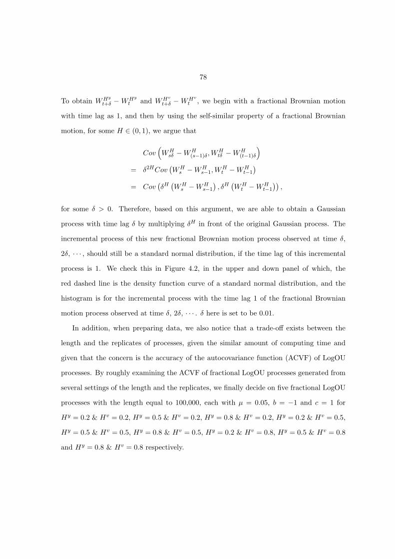
78
To obtain WHy
t+δ −WHy
t and WHv
t+δ −WHv
t , we begin with a fractional Brownian motion
with time lag as 1, and then by using the self-similar property of a fractional Brownian
motion, for some H ∈ (0, 1), we argue that
Cov(WH
sδ −WH(s−1)δ,W
Htδ −WH
(t−1)δ
)
= δ2HCov(WH
s −WHs−1,W
Ht −WH
t−1
)
= Cov(δH(WH
s −WHs−1
), δH
(WH
t −WHt−1
)),
for some δ > 0. Therefore, based on this argument, we are able to obtain a Gaussian
process with time lag δ by multiplying δH in front of the original Gaussian process. The
incremental process of this new fractional Brownian motion process observed at time δ,
2δ, · · · , should still be a standard normal distribution, if the time lag of this incremental
process is 1. We check this in Figure 4.2, in the upper and down panel of which, the
red dashed line is the density function curve of a standard normal distribution, and the
histogram is for the incremental process with the time lag 1 of the fractional Brownian
motion process observed at time δ, 2δ, · · · . δ here is set to be 0.01.
In addition, when preparing data, we also notice that a trade-off exists between the
length and the replicates of processes, given the similar amount of computing time and
given that the concern is the accuracy of the autocovariance function (ACVF) of LogOU
processes. By roughly examining the ACVF of fractional LogOU processes generated from
several settings of the length and the replicates, we finally decide on five fractional LogOU
processes with the length equal to 100,000, each with µ = 0.05, b = −1 and c = 1 for
Hy = 0.2 & Hv = 0.2, Hy = 0.5 & Hv = 0.2, Hy = 0.8 & Hv = 0.2, Hy = 0.2 & Hv = 0.5,
Hy = 0.5 & Hv = 0.5, Hy = 0.8 & Hv = 0.5, Hy = 0.2 & Hv = 0.8, Hy = 0.5 & Hv = 0.8
and Hy = 0.8 & Hv = 0.8 respectively.

79
Figure 4.2 Check on the random drivers
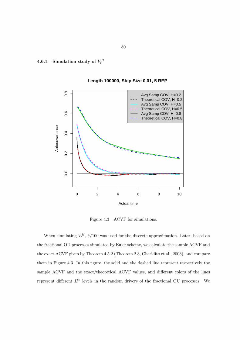
80
4.6.1 Simulation study of V Ht
0 2 4 6 8 10
0.0
0.2
0.4
0.6
0.8
Length 100000, Step Size 0.01, 5 REP
Actual time
Aut
ocov
aria
nce
Avg Samp COV, H=0.2Theoretical COV, H=0.2Avg Samp COV, H=0.5Theoretical COV, H=0.5Avg Samp COV, H=0.8Theoretical COV, H=0.8
Figure 4.3 ACVF for simulations.
When simulating V Ht , δ/100 was used for the discrete approximation. Later, based on
the fractional OU processes simulated by Euler scheme, we calculate the sample ACVF and
the exact ACVF given by Theorem 4.5.2 (Theorem 2.3, Cheridito et al., 2003), and compare
them in Figure 4.3. In this figure, the solid and the dashed line represent respectively the
sample ACVF and the exact/theoretical ACVF values, and different colors of the lines
represent different Hv levels in the random drivers of the fractional OU processes. We
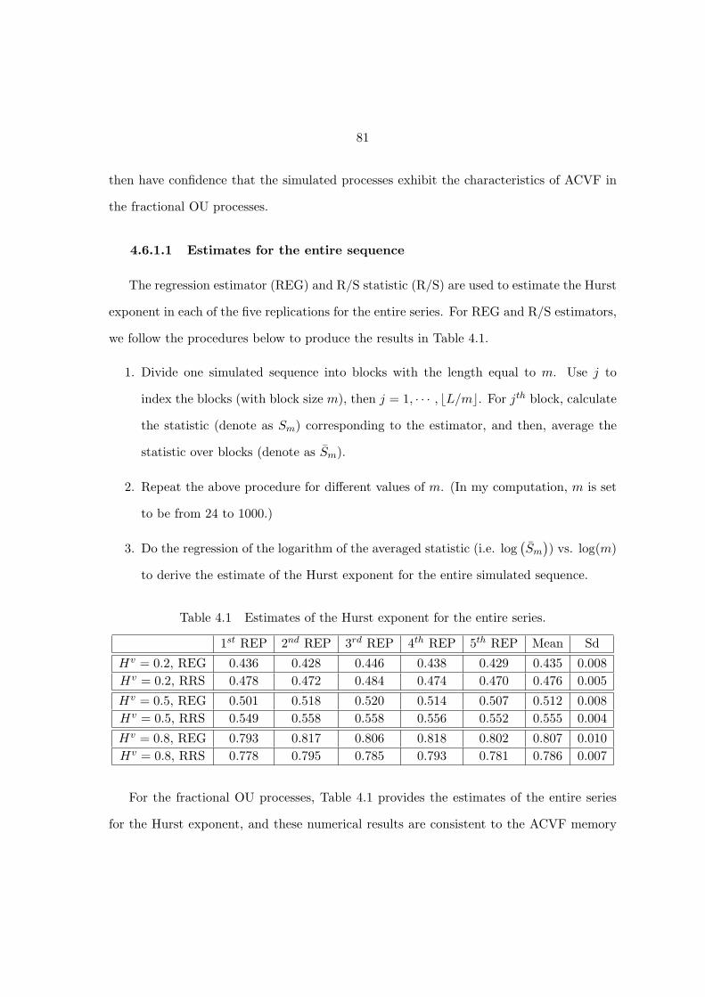
81
then have confidence that the simulated processes exhibit the characteristics of ACVF in
the fractional OU processes.
4.6.1.1 Estimates for the entire sequence
The regression estimator (REG) and R/S statistic (R/S) are used to estimate the Hurst
exponent in each of the five replications for the entire series. For REG and R/S estimators,
we follow the procedures below to produce the results in Table 4.1.
1. Divide one simulated sequence into blocks with the length equal to m. Use j to
index the blocks (with block size m), then j = 1, · · · , ⌊L/m⌋. For jth block, calculate
the statistic (denote as Sm) corresponding to the estimator, and then, average the
statistic over blocks (denote as Sm).
2. Repeat the above procedure for different values of m. (In my computation, m is set
to be from 24 to 1000.)
3. Do the regression of the logarithm of the averaged statistic (i.e. log(Sm
)) vs. log(m)
to derive the estimate of the Hurst exponent for the entire simulated sequence.
Table 4.1 Estimates of the Hurst exponent for the entire series.
1st REP 2nd REP 3rd REP 4th REP 5th REP Mean Sd
Hv = 0.2, REG 0.436 0.428 0.446 0.438 0.429 0.435 0.008
Hv = 0.2, RRS 0.478 0.472 0.484 0.474 0.470 0.476 0.005
Hv = 0.5, REG 0.501 0.518 0.520 0.514 0.507 0.512 0.008
Hv = 0.5, RRS 0.549 0.558 0.558 0.556 0.552 0.555 0.004
Hv = 0.8, REG 0.793 0.817 0.806 0.818 0.802 0.807 0.010
Hv = 0.8, RRS 0.778 0.795 0.785 0.793 0.781 0.786 0.007
For the fractional OU processes, Table 4.1 provides the estimates of the entire series
for the Hurst exponent, and these numerical results are consistent to the ACVF memory

82
analysis in Proposition 4.1. In other words, when Hv is no more than 0.5, the estimates
tend to be around or below 0.5, and when Hv is larger than 0.5, the estimates are greater
than 0.5.
4.6.1.2 Block effect
We then follow Peters (1996) to study the effect of the maximum block size on the
estimates of the Hurst exponent, and this effect is called as block effect. The results for the
maximum block size values taken on 100, 200, · · · , 1000, are shown in Figure 4.4, of which
the x-axis is the maximum block size, and y-axis is the estimate of the Hurst exponent.
200 400 600 800 1000
0.3
0.4
0.5
0.6
0.7
0.8
0.9
1.0
Nominal H=0.2,0.5,0.8, 5 REP, Length 100000
ith Blk Size
Val
ues
of H
_hat
Nominal H=0.2Nominal H=0.5Nominal H=0.8
REG ESTR/S EST
Figure 4.4 Block effect on the estimates of the Hurst exponent.
This figure implies that the Hurst exponent changes around a certain value (not nec-
essarily to be the Hv value), and shows no block effect in the fractional OU processes.
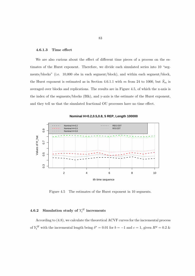
83
4.6.1.3 Time effect
We are also curious about the effect of different time pieces of a process on the es-
timates of the Hurst exponent. Therefore, we divide each simulated series into 10 “seg-
ments/blocks” (i.e. 10,000 obs in each segment/block), and within each segment/block,
the Hurst exponent is estimated as in Section 4.6.1.1 with m from 24 to 1000, but Sm is
averaged over blocks and replications. The results are in Figure 4.5, of which the x-axis is
the index of the segments/blocks (Blk), and y-axis is the estimate of the Hurst exponent,
and they tell us that the simulated fractional OU processes have no time effect.
2 4 6 8 10
0.3
0.5
0.7
0.9
Nominal H=0.2,0.5,0.8, 5 REP, Length 100000
ith time sequence
Val
ues
of H
_hat
Nominal H=0.2Nominal H=0.5Nominal H=0.8
REG ESTR/S EST
Figure 4.5 The estimates of the Hurst exponent in 10 segments.
4.6.2 Simulation study of Y Ht increments
According to (4.8), we calculate the theoretical ACVF curves for the incremental process
of Y Ht with the incremental length being δ∗ = 0.01 for b = −1 and c = 1, given Hy = 0.2 &
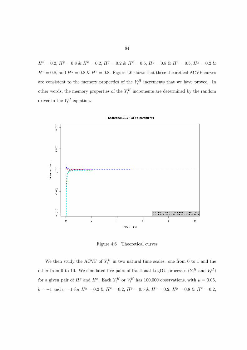
84
Hv = 0.2, Hy = 0.8 & Hv = 0.2, Hy = 0.2 & Hv = 0.5, Hy = 0.8 & Hv = 0.5, Hy = 0.2 &
Hv = 0.8, and Hy = 0.8 & Hv = 0.8. Figure 4.6 shows that these theoretical ACVF curves
are consistent to the memory properties of the Y Ht increments that we have proved. In
other words, the memory properties of the Y Ht increments are determined by the random
driver in the Y Ht equation.
0 2 4 6 8 1 0−0 .010 −0 .0050 .0000 .0050 .010 T h e o r e t i c a l A C V F o f Y t i n c r e m e n t s
A c t u a l T i m eA ut ocovari ance
H y = 0 . 2 , H v = 0 . 2H y = 0 . 8 , H v = 0 . 2 H y = 0 . 2 , H v = 0 . 8H y = 0 . 8 , H v = 0 . 8 H y = 0 . 2 , H v = 0 . 5H y = 0 . 8 , H v = 0 . 5Figure 4.6 Theoretical curves
We then study the ACVF of Y Ht in two natural time scales: one from 0 to 1 and the
other from 0 to 10. We simulated five pairs of fractional LogOU processes (Y Ht and V H
t )
for a given pair of Hy and Hv. Each Y Ht or V H
t has 100,000 observations, with µ = 0.05,
b = −1 and c = 1 for Hy = 0.2 & Hv = 0.2, Hy = 0.5 & Hv = 0.2, Hy = 0.8 & Hv = 0.2,

85
Hy = 0.2 & Hv = 0.5, Hy = 0.5 & Hv = 0.5, Hy = 0.8 & Hv = 0.5, Hy = 0.2 & Hv = 0.8,
Hy = 0.5 & Hv = 0.8 and Hy = 0.8 & Hv = 0.8 respectively. The recorded time lag (or
step size), denoted by δ, is set to be 0.01 as well as the length of the increments (δ∗). The
lags of ACVF are then computed at 0.01, 0.02, · · · , 100×0.01 = 1 in Figure 4.7 - 4.9, while
the lags are at 0.1, 0.2, · · · , 1000 × 0.01 = 10 in Figure 4.10 - 4.12. The upper panel in
each figure includes ACVF curves for both the V Ht and the Y H
t increments for three pairs
of Hy and Hv values, and the down panel shows ACVF for the Y Ht increments only and
with a smaller scale in the y-axis than the upper panel.
Figure 4.7 ACVF on the real time interval (0, 1) for Hv = 0.2
4.6.2.1 Discussion on the simulation results for ACVF
Since in the simulation, Y Ht has fixed time lag δ and increment length δ∗ being a
multiple of δ, we denote the ACVF of Y Ht increments as γ(kδ; δ∗ = k0δ,H
y, Hv) for the
lag value kδ with k, k0 ∈ Z+. We can show the following proposition for the theoretical

86
Figure 4.8 ACVF on the real time interval (0, 1) for Hv = 0.5
Figure 4.9 ACVF on the real time interval (0, 1) for Hv = 0.8

87
Figure 4.10 ACVF on the real time interval (0, 10) for Hv = 0.2
Figure 4.11 ACVF on the real time interval (0, 10) for Hv = 0.5

88
Figure 4.12 ACVF on the real time interval (0, 10) for Hv = 0.8
ACVF curves of the increments with a certain δ.
Proposition 4.6.1 Given Hy, Hv, k0 and k, when δ increases, |γ(kδ; k0δ,Hy, Hv)| in-
creases.
Proof. Recall that, for k ∈ R+,
γ(kδ; k0δ,Hy, Hv) = Cov
(∆Y H
0 ,∆Y Hkδ
)
= Cov(eV
H0 ∆WHy
0 , eVHkδ ∆WHy
kδ
)
= E(∆WHy
0 ∆WHy
kδ
)E(eV
Hkδ +V H
0
)
= E(∆WHy
0 ∆WHy
kδ
)eV ar(V H
0 )+Cov(V Hkδ ,V H
0 )
= ec2
Γ(2Hv+1) sin(πHv)π
∞∫0
1+cos(kδx) |x|1−2Hv
|b|2+x2 dxE(∆WHy
0 ∆WHy
kδ
)
= 0.5ec2
Γ(2Hv+1) sin(πHv)π
∞∫0
1+cos(kδx) |x|1−2Hv
|b|2+x2 dx
×(|kδ + k0δ|2Hy
+ |kδ − k0δ|2Hy − 2 |kδ|2Hy).

89
For δ1 < δ2,
0 ≤ |γ(kδ1; k0δ1, Hy, Hv)|
|γ(kδ2; k0δ2, Hy, Hv)| =δ2Hy
1
δ2Hy
2
< 1.
In Figure 4.6, we observed that
Proposition 4.6.2 Given δ, Hy, k0 and k, when Hv increases, |γ(kδ; k0δ,Hy, Hv)| in-
creases.
Proof. Given the values of δ, Hy, k0 and k,
|γ(kδ; k0δ,Hy, Hv)| = a positive constant × eV ar(V H
0 )+Cov(V Hkδ ,V H
0 )
From Figure 4.3, we observe the fact that∣∣V ar
(V H
0
)∣∣ and∣∣Cov
(V H
kδ , VH0
)∣∣ increase, as Hv
increases, for k ∈ Z+, then it is obvious that |γ(kδ; k0δ,H
y, Hv)| increases as Hv increases.
From Figure 4.7 to Figure 4.12, we observed the following things for ACVF of the Y Ht
increments.
• When Hy = 0.8, the ACVF curve of the Y Ht increments takes on the positive values
and converges to zero. When Hy = 0.2, the ACVF curve converges to zero from the
negative values, while Hy = 0.5, the ACVF curve is almost on the x-axis all the time.
The proposition below explains this phenomenon.
Proposition 4.6.3 Given δ and Hv, when Hy > 0.5, Hy < 0.5 and Hy = 0.5, we
have γ(kδ; k0δ,Hy, Hv) > 0, γ(kδ; k0δ,H
y, Hv) < 0, γ(kδ; k0δ,Hy, Hv) = 0 respec-
tively.

90
Proof.
γ(kδ; k0δ,Hy, Hv)
= E(∆WHy
0 ∆WHy
kδ
)eV ar(V H
0 )+Cov(V Hkδ ,V H
0 )
= ec2
Γ(2Hv+1) sin(πHv)π
∞∫0
1+cos(kδx) |x|1−2Hv
|b|2+x2 dxE(∆WHy
0 ∆WHy
kδ
)
= a positive function of kδ × E(∆WHy
0 ∆WHy
kδ
).
Therefore, when Hy > 0.5 , Hy < 0.5 and Hy = 0.5, we have E(∆WHy
0 ∆WHy
kδ
)
positive, negative and equal to 0 respectively, and then similar to γ(kδ; k0δ,Hy, Hv).
Remark 4.6.4 Here, we also discuss the convergent speed for different Hy val-
ues. When kδ > 0 is large, we know that E(∆WHy
0 ∆WHy
kδ
)∼ O
((kδ)2Hy−2
)and
Cov(V H
kδ , VH0
)∼ O
((kδ)2Hv−2
). Thereby, γ(kδ; k0δ,H
y, Hv) ∼ O((kδ)2Hy−2
). In
other words, the convergent speed is mainly determined by the Y Ht random driver
process, or Hy, i.e. the larger the Hy is, the more slowly the process converges.
• The ACVF curve of the Y Ht increments forHv = 0.8 tends to have a larger magnitude
in fluctuations than Hv = 0.2.
Argument: We recall that in the theoretical expression of ACVF for the Y Ht incre-
ments, the part including Hv is the power of the exponential function, which is in
the form of ACVF of V Ht . In the simulation, we also notice that the sample ACVF
of V Ht averaged over 5 samples, tends to have larger variance with Hv = 0.8 than
with Hv = 0.5 or Hv = 0.2, which may cause the larger magnitude in fluctuations
for the ACVF curve of the Y Ht increments for Hv = 0.8. As to the reason of that
the sample ACVF of V Ht averaged over 5 samples has larger variance with Hv = 0.8

91
than with Hv = 0.5 or Hv = 0.2, it could be a research interest but currently is not
the focus of our study.
4.6.2.2 Discussion on Y Ht increments
Moreover, we simulate data more carefully to study H. The data are still five pairs of
fractional LogOU processes (Y Ht and V H
t ) for a given pair of Hy and Hv. The recorded
time lag (or step size) is again set to be δ = 0.01, but more considerately, δ/100 is used
for the discrete approximation. Therefore, to have similar amount of computational work,
each Y Ht or V H
t currently has 100,000 observations with µ = 0.05, b = −1 and c = 1 for
Hy = 0.2 & Hv = 0.2, Hy = 0.5 & Hv = 0.2, Hy = 0.8 & Hv = 0.2, Hy = 0.2 & Hv = 0.5,
Hy = 0.5 & Hv = 0.5, Hy = 0.8 & Hv = 0.5, Hy = 0.2 & Hv = 0.8, Hy = 0.5 & Hv = 0.8
and Hy = 0.8 & Hv = 0.8 respectively. The incremental length (δ∗) of Y Ht is still 0.01,
and the actual time length for the simulated fractional OU processes is then equal to 1000.
In Table 4.2, we see that whether H estimates for the Y Ht increments are greater
than, around or smaller than 0.5, is determined by Hy value in the random drivers of Y Ht
processes. This notice is consistent to what we have proven for the Y Ht increments. Figure
4.13 and Figure 4.14 show that there are no block or time effects in the Y Ht increments.
However, we realize that the H estimates are neither the Hy value nor the Hv value.
Further, the relationship between the H estimates and the Hy value or the Hv value has
not been studied yet and could be a research topic, but currently not the focus of this
study.
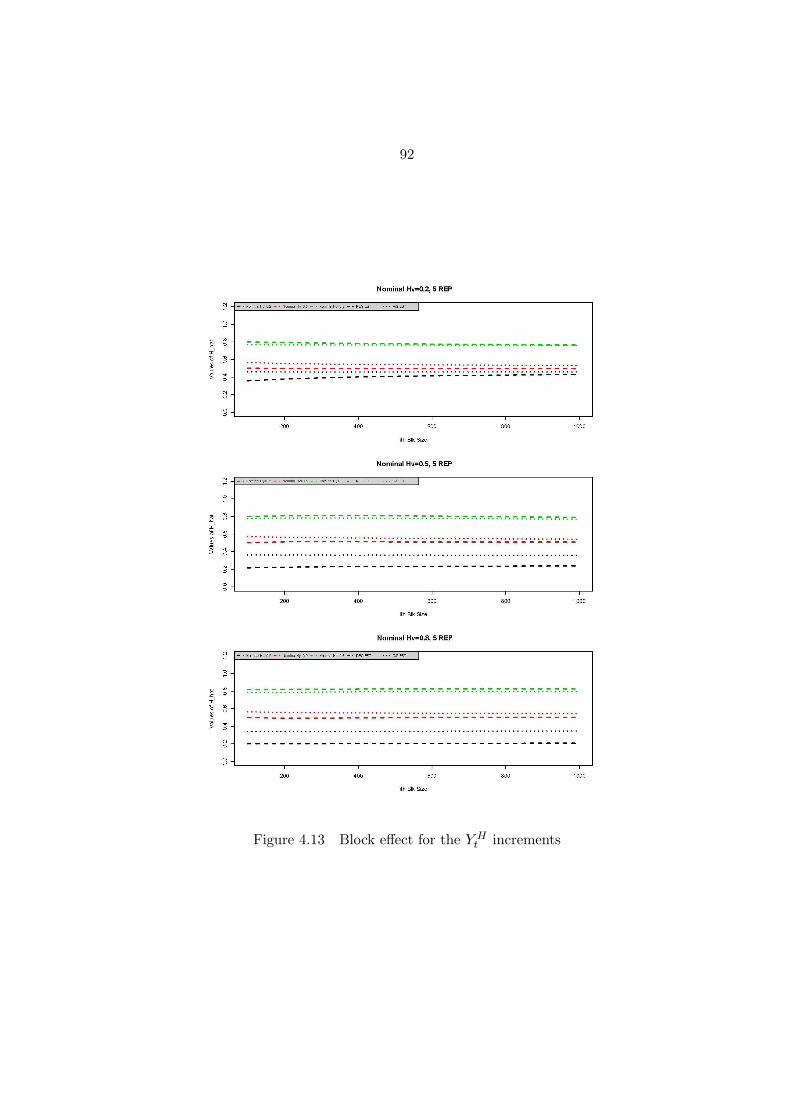
92
Figure 4.13 Block effect for the Y Ht increments

93
Figure 4.14 Time effect for the Y Ht increments

94
Table 4.2 Estimates of the Hurst exponent for the Y Ht incremental process.
EST 1st REP 2nd REP 3rd REP 4th REP 5th REP MEAN SD
REG 0.423 0.428 0.437 0.430 0.426 0.429 0.005Hy = 0.2RRS 0.457 0.461 0.457 0.454 0.462 0.458 0.003REG 0.485 0.503 0.515 0.485 0.488 0.495 0.013Hv = 0.2 Hy = 0.5RRS 0.528 0.531 0.540 0.530 0.525 0.531 0.006REG 0.748 0.750 0.764 0.780 0.781 0.765 0.016Hy = 0.8RRS 0.754 0.752 0.759 0.759 0.772 0.759 0.008REG 0.238 0.247 0.239 0.239 0.231 0.239 0.006Hy = 0.2RRS 0.360 0.366 0.357 0.360 0.355 0.360 0.004REG 0.504 0.513 0.506 0.531 0.494 0.509 0.014Hv = 0.5 Hy = 0.5RRS 0.540 0.544 0.533 0.550 0.545 0.542 0.006REG 0.778 0.798 0.756 0.823 0.794 0.790 0.025Hy = 0.8RRS 0.770 0.770 0.760 0.780 0.764 0.769 0.007REG 0.201 0.209 0.217 0.200 0.227 0.211 0.011Hy = 0.2RRS 0.344 0.344 0.344 0.353 0.346 0.346 0.004REG 0.476 0.512 0.519 0.523 0.470 0.500 0.025Hv = 0.8 Hy = 0.5RRS 0.540 0.544 0.552 0.549 0.533 0.543 0.008REG 0.838 0.754 0.862 0.816 0.791 0.812 0.042Hy = 0.8RRS 0.808 0.782 0.789 0.797 0.794 0.794 0.009
4.7 Fractional Cox-Ingersoll-Ross (CIR) Model
4.7.1 The well-definedness of the fractional CIR model system
The solution to the CIR model with the random driver in Vt being a fBm, has not been
discussed extensively in literature. Below, we follow the idea of solving the CIR model
with a BM as the random driver, and see how further we can get for the CIR with a fBm.
A pathwise solution of CIR model can be generated as follows (Shreve, 2004).
Define
y˜
t =
X1,t
...
Xd,t
, y˜
0 =
X1,0
...
Xd,0
, t0 = 0, A =
b
2, f(t) =
c
2,W˜t =
dW1,t
...
dWd,t
,
for b < 0, c > 0, and d ≥ 1, and then, the Ornstein-Uhlenbeck (OU) functions
dXj,t =b
2Xj,tdt+
c
2dWj,t, j = 1, · · · , d

95
can be expressed as
dy˜
t = Ay˜
tdt+ f(t)dW˜t,
and the solution in the vector form should be
y˜
t = e(t−t0)Ay˜
0 +
t∫
t0
e(t−s)Af(s)dW˜s.
In other words, the solution is
X1,t
...
Xd,t
= ebt2
X1,0
...
Xd,0
+c
2
t∫0
e(t−u)b/2dW1,u
...t∫0
e(t−u)b/2dWd,u
,
based on which, people define
a = dc2/4
Vt =d∑
j=1X2
j,t
Wt =d∑
j=1
t∫0
Xj,s√VsdWj,s
(4.9)
and, by the martingale property of BM and Levy’s Theorem, check that Wt is still a
Brownian motion and Vt is the pathwise solution for the CIR model with this BM as the
random driver (dVt = (a+ bVt)dt+ c√VtdWt).
If the random driver is fBm in the volatility equation, to get the solution to the d-
dimensional fractional OU functions in the similar way, it would be
XH1,t
...
Xhd,t
= ebt2
XH1,0
...
XHd,0
+c
2
t∫0
e(t−u)b/2dWH1,u
...t∫0
e(t−u)b/2dWHd,u
.

96
Now, if we still want to use V Ht =
d∑j=1
(XH
j,t
)2as the solution, we need to check that
d∑j=1
t∫0
Xj,s√V H
s
dWHj,s is a fBm, which becomes difficult since fBm is usually not a martingale.
The form of the CIR solution with fBm as the random driver is then unclear, and later, we
focus on the price equation with a fractional Brownian motion as the random driver and
the volatility equation with a regular BM as the random driver by following the notations
in the equation (4.5).
Theorem 4.7.1 Define fractional CIR dynamic model system as
dY Ht = µdt+
√VtdW
Hy
t , dVt = κ(θ − Vt)dt+ σv
√VtdWt,
where WHy
t is a fBm with index Hy and V ar(WHy
1
)= 1, Wt is a standard BM independent
of WHy
t , and κ > 0, θ < 0, σv > 0. Then, this dynamic model system is well defined for
Hy ∈ [0.5, 1).
Proof. The crucial part of the proof for this theorem is still the price equation. Further,
similar to Theorem 4.5.4, after reparameterizing dVt = κ(θ−Vt)dt+σv
√VtdWt into dVt =
(a + bVt)dt + c√VtdWt for a = κθ, b = −κ and c = σv, and by the equation (4.9) and
the mean value theorem in several variables, the pathwise solution of CIR equation (Vt)
obtained in the corresponding way has the p-variation featured similarly to the p-variation
of the solutions of the OU functions, and thus has a finite p-variation if p ≥ 10.5 = 2.
Following the p-variation condition for well-definedness of pathwise solution of stochastic
integral with respect to a fractional Brownian motion, we have (1 −Hy)−1 ≥ 2 and thus
obtain the theorem.

97
4.7.2 The joint behavior of Y Ht and Vt
To understand the joint behavior in the memory structure of the pricing and volatility
processes in CIR model, we review some existing results (Cox et al., 1985a, 1985b), and
then provide a proposition for the memory features of Y Ht and Vt.
Following the commonly used notations for CIR model, the fractional Cox-Ingersoll-
Ross (CIR) model system can be written as
dY Ht = µdt+
√VtdW
Hy
t ,
dVt = κ(θ − Vt)dt+ σv
√VtdWt,
whereWHy
t is a fBm with indexHy and V ar(WHy
1
)= 1, Wt is a standard BM independent
of WHy
t , and κ > 0, θ < 0, σv > 0.
Fact I: (Cox et al.,1985b) The distribution of Vs given Vt for s > t is a non-central
chi-square,
2cVs|Vt ∼ χ2(2q + 2, 2u),
for c = 2κ/σ2v(1 − e−κ(s−t)), non-centrality parameter u = cVte
−κ(s−t), and degrees of
freedom q = 2κθσ2
v− 1. As s becomes large, Vs|Vt goes to a Gamma distribution with
parameters (2κθσ2
v, 2κ
σ2v). The stationary marginal distribution of the Vs process is the same
Gamma distribution with mean θ and variance θσ2v
2κ .
Fact II: (Cox et al.,1985b) Straightforward calculations to obtain the expected value
and variance of Vs given Vt, for s ≥ t, show that:
E(Vs|Vt) = Vte−κ(s−t) + θ(1 − e−κ(s−t)),
V ar(Vs|Vt) = Vtσ2
v
κ
(e−κ(s−t) − e−2κ(s−t)
)+ θ
σ2v
2κ
(1 − e−κ(s−t)
)2.
(4.10)
98
If t = 0, then
E(Vs|V0) =V0e−κs + θ(1 − e−κs),
V ar(Vs|V0) = V0σ2
v
κ(e−κs − e−2κs) + θ
σ2v
2κ(1 − e−κs)2
= θσ2
v
2κ+σ2
v
κ(V0 − θ)e−κs +
σ2v
κ
(θ
2− V0
)e−2κs.
(4.11)
In the remainder, we still assume that s > t and s− t = h > 0. Then, for the volatility
process (Vt) and the price process (Y Ht ), we can derive the following proposition about
their covariance structure and about their memory structure.
Proposition 4.7.2 For well-defined fractional CIR dynamic model system,
dY Ht = µdt+
√VtdW
Hy
t ,
dVt = κ(θ − Vt)dt+ σv
√VtdWt,
where WHy
t is a fBm with index Hy and V ar(WHy
1
)= 1, Wt is a standard BM independent
of WHy
t , and κ > 0, θ < 0, σv > 0, we have
1. Vt process (and also its incremental process) has a short time memory.
2. the memory structure of ∆Y Ht := µ∆ + eVt∆WHy
t depends on Hy, i.e. a short time
memory, a long time memory or no memory for 0 < Hy < 0.5, 0.5 < Hy < 1 or
Hy = 0.5 respectively.
Proof.
1. For the stationary process Vt and h = s− t > 0, it is easy to check that
E(VsVt) = E(VtE(Vs|Vt)) = E(Vt
(Vte
−κ(s−t) + θ(1 − e−κ(s−t))))
= θ2+θσ2
v
2κe−κ(s−t),

99
and EVt = θ. Therefore, we can obtain that
Cov(Vt, Vs) =θσ2
v
2κe−κ(s−t),
Cov(∆Vt,∆Vs) =θσ2
v
2κ
(2e−κ(s−t) − e−κ(s−t−δ) − e−κ(s−t+δ)
)
=θσ2
v
2κ(2e−κh − e−κ(h−δ) − e−κ(h+δ)) := C1e
−κh,
where the constant C1 is defined as (2 − eκδ − e−κδ) θσ2v
2κ , and
∞∑
h=1
|Cov(Vt, Vt+h)| =θσ2
v
2κ
∞∑
h=1
e−κh <∞,
∞∑
h=1
|Cov(∆Vt,∆Vt+h)| = |C1|∞∑
h=1
e−κh <∞.
We then conclude that the process Vt (and also its incremental process) has a short
time memory.
2. We approximate the pricing model
dY Ht = µdt+
√VtW
Hy
t ,
where WHy
t is fractional Brownian motion, by
∆Y Ht := µ+
√Vt∆W
Hy
t
for ∆WHy
t := WHy
t+1−WHy
t which is fractional Gaussian noise corresponding to WHy
t .
Further, since the process WHy
t is independent of the process Vt, we obtain that
E(√Vt∆W
Hy
t ) = E√VtE∆WHy
t = 0,
and
Cov(∆Y Ht ,∆Y H
s )
= Cov(√
Vt∆WHy
t ,√Vs∆W
Hy
s
)= E(
√Vt∆W
Hy
t
√Vs∆W
Hy
s )
= E(∆WHy
t ∆WHy
s )E(√
Vt
√Vs
)= γHy(s− t)E
√VtVs,
100
where γHy(s) = 12
(|s+ δ|2Hy
+ |s− δ|2Hy − 2|s|2Hy)is the ACVF of a fractional
Gaussian noise with the self-similarity index Hy and the time lag of the fractional
Brownian motion (corresponding to this fGn) as δ. Consequently,
• if Hy = 0.5, for s 6= t, Cov(∆Y Ht ,∆Y H
s ) = 0 and ∆Y Ht is a random walk.
• if 0 < Hy < 0.5,
0 ≤ |Cov(∆Y Ht ,∆Y H
s )| ≤ |γHy(s− t)| E(Vt)12 E(Vs)
12 = |γHy(s− t)| θ,
and∞∑
h=1
|Cov(∆Y Ht ,∆Y H
t+h)| <∞,
meaning that ∆Y Ht has a short memory.
• if 0.5 < Hy < 1, we first define the quantities and check the facts below:
– 2c1Vs|Vt ∼ χ2(2q + 2, 2ut), for s − t = h > 0, c1 = 2κσ2
v(1−e−κh), ut =
2κσ2
v
e−κh
1−e−κhVt, and q = 2κθσ2
v− 1.
– c3 = c1e−κh, and c4 = c3
c2= 1−e−κt
1−e−κh e−κh > 0.
– Given a random variable X following a non-central χ2(K,λ) with degrees
of freedom K > 0 and non-centrality parameter λ > 0, its density function
is given by
fX(x) =e−
λ+x2
2K2
∞∑
j=0
(λ
4
)j xK2
+j−1
j!Γ(
K2 + j
) ,
and
E(X
12
)=
√2e−
λ2
∞∑
j=0
(λ2
)jΓ(
K+2j+12
)
j!Γ(
K+2j2
) .
– The fractional moment of a random variable X following a Gamma distri-
bution with mean α/β and variance α/β2 for j ≥ 0 and a constant a > 0,
is given by

101
E(Xj+0.5e−aX
)=
βαΓ(α+ j + 0.5)
(β + a)α+j+0.5Γ(α).
Then, for h = s− t > 0,
E√VtVs =
1√2c1
E√VtE
(√2c1Vs|Vt
)
=1√2c1
E
√2Vte
−ut
∞∑
j=0
ujt
j!
Γ(q + j + 1.5)
Γ(q + j + 1)
≥ 1√c1
Γ(q + 1.5)
Γ(q + 1)E(√
Vte−utuj
t
)
≥ 1√c1
(Γ(q + 1.5)
Γ(q + 1)
)2(σ2v
2κ
)0.5
(1 − e−κh)q+1.5
≥(
Γ(q + 1.5)
Γ(q + 1)
)2(σ2v
2κ
)(1 − e−κh)q+2
Therefore, for 0.5 < Hy < 1,
Cov(∆Y Ht ,∆Y H
t+h) = γHy(s−t)E√VtVs ≥ γHy(s−t)σ
2v
2κ(1−e−κh)q+2
(Γ(q + 1.5)
Γ(q + 1)
)2
,
and∞∑
h=1
∣∣Cov(∆Y Ht ,∆Y H
t+h)∣∣ =
∞∑
h=1
Cov(∆Y Ht ,∆Y H
t+h) = ∞.
4.8 Future Work
4.8.1 Time-varying structure
Motivated by the study of S&P500, stochastic volatility models with time-varying mem-
ory structures are interesting future topics. To help with this type of research, processes
102
with time-varying memory structure should be proposed or studied. Therefore, as the
basis of future study, a Gaussian process with changed values of H are introduced below.
(Ayache et al., 2000.)
• Definition 4.8.1 (Holder Function of Exponent H) Let (X, dX) and (Y, dY ) be two
metric spaces. A function F : X → Y is called a Holder function of exponent h ≥ 0,
if for each x, y ∈ X such that dX(x, y) < 1, we have
dY (F (x), F (y)) ≤ kdX(x, y)h
for x, y ∈ X and some constant k > 0. (Lutton and Levy Vehel, 1998.)
• Definition 4.8.2 Let H : [0,∞) → [a, b] ⊂ (0, 1) be a Holder function of exponent
β > 0.
– (Moving Average Definition) For t ≥ 0, the following random function is called
multifractional Brownian motion (mBm) with functional parameter H (W de-
notes ordinary Brownian motion):
WH(t)(t) =
∫ 0
−∞[(t− s)H(t)−1/2 − (−s)H(t)−1/2]dW (s)+
∫ t
0(t− s)H(t)−1/2dW (s).
– (Harmonizable Representation) For t ≥ 0, the following function is called mul-
tifractional Brownian motion:
WH(t)(t) =
∫
R
eitξ−1
|ξ|H(t)+1/2dW (ξ).
Contrarily to fBm, the almost sure Holder exponent of mBm is allowed to vary along
the trajectory, a useful feature when one needs to model processes whose regularity
evolves in time. Following the moving average definition or the Harmonizable rep-
resentation of mBm, this process is a zero mean Gaussian process whose increments

103
are in general neither independent nor stationary. When H(t) = H for all t, mBm
degenerates to fBm with the exponent H. Since the incremental process of mBm in
general are not stationary, it is not likely to define stochastic integrals for mBm in
general, but only for some specific forms of the function H(t), e.g. a step function.
• Moreover, the covariance structure of mBm is stated in following proposition (Ayache
et al., 2000).
Proposition 4.8.3 Let X(t) be a standard mBm (i.e. such that the variance at t = 1
is 1) with functional parameter H(t). Then,
Cov(X(t), X(s)) = E(X(t)X(s)) = D(H(t), H(s))(tH(t)+H(s)+sH(t)+H(s)−|t−s|H(t)+H(s)),
where
D(x, y) =
√Γ(2x+ 1)Γ(2y + 1) sin(πx) sin(πy)
2Γ(x+ y + 1) sin(π(x+ y)/2).
4.8.2 Dependent WHy
t and WHv
t or Wt
If we relax the assumption of independence of WHy
t and WHv
t or Wt, some of the
results proved in Section 4.5.2 and Section 4.7.2 hold. In particular, results regarding the
covariance of V Ht or Vt do not change. However, results pertaining to Y H
t need to be
revised. The dependence between W yt and W ν
t can also take on different forms and induce
different types of interactions between Y Ht and V H
t or Vt. For example, it has been argued
that minor disturbances in the V Ht or Vt process can introduce a delayed effect in the Y H
t
process.

104
CHAPTER 5. SUMMARY AND CONCLUSIONS
The R/S statistic that defines the Hurst exponent is often used to determine the long-
range dependence in a time series. The self-similarity index defined with a process, de-
termines the memory structure underlying a self-similar process. This dissertation shows
that asymptotically, the R/S statistic and the self-similarity index of fractional Brownian
motion agree in the expectation sense. This result has been mentioned in the literature
but – to our knowledge – without formal proof, see, e.g., Taqqu et al. (1995).
In addition to the R/S statistic, many other estimators of the self-similarity index in
fractional Brownian motion have been proposed in the literature. Two of those are based
on the aggregated variance of the process. We show that for a fixed number of blocks
(with fixed block size), the Aggregated Variance Method (AVM) and the Absolute Value
of the Aggregated Series (AVA) method result in estimators of H that converge to H with
probability 1. Therefore, both estimators are consistent. To prove these results we have
fixed both the number of blocks and the block size. It is possible to show that both results
still hold if block size and number are not fixed, as long as they are bounded. Our proof
does not extend in a natural way to the situation where either block size or block number
become unbounded. From a practical viewpoint, this does not constitute a limitation of
these approaches if we are interested in the statistics of observed data series.
We studied the properties of several estimators of the self-similarity index that are
mentioned in literature. We used fractional Gaussian noise with different values of H to

105
be our test processes, and examined the sample variance, the bias and the mean square
error of these estimators. The results of our simulation experiment suggest that estimators
based on the aggregated data behave well, while the Whittle estimator (WHI) and the
regression estimator (REG) also show nice properties.
We then investigated the effect of block size on the H and the time-dependence of the
estimated H. This time we adopted a real time series, the S&P500, to be our test process.
One reason to use the S&P500, is that our final interest is in learning about and modeling
real data. The S&P500 has studied extensively and it has been found that the estimates of
its underlying memory structure may be affected by block size effects. For example, Peters
(1996) found that the memory structure of the monthly S&P500 stock price series follows a
curve with a peak around block sizes equal to four years. We used the S&P500 weekly price
series instead, and applied the regression estimator which showed nice properties in the
earlier simulation study and which is easy to implement. To make our results comparable
to Peters findings, we also applied the empirical R/S and the R/S statistic to these weekly
price data. Besides investigating the block-size effect and the time effect on the estimated
H, we also studied the memory structure of these data using a permutation test. From our
results, we see that the S&P 500 price data behave more like a random walk or a short time
memory process with short or very long block size, but exhibit a long-memory property in
the medium block-size range, and shows a decreasing time effect.
As a final remark, this work also focused on some of the standard continuous-time
models for a process with a short time memory structure. In particular, after an extensive
review of the literature we found that few authors have discussed checking the memory
structure of complex continuous-time market models. For long memory processes, the
discussion about continuous-time market models in the literature is even less abundant.
To fill this gap, this dissertation also provides some results in the area of continuous-time

106
models with long time memory where the long memory is incorporated into the main
process,i.e. the price process. These long memory processes do not necessarily capture
time-dependence in the memory coefficient H. There are some stochastic processes that
have a time dependent H including multifractional Brownian motion (mBm), but how to
develop a dynamical model for processes with time dependent H process is still an open
question that deserves more research.
107
BIBLIOGRAPHY
Adler, R. J. (1990). An Introduction to Continuity, Extrema, and Related Topics for Gen-
eral Gaussian Processes. Institute of Mathematical Statistics, Hayward, CA.
Ayache, A, Cohen, S., and Levy-Vehel, J. (2000). Covariance structure of multifractional
Brownian motion, with application to long range dependence. ICASSP IEEE Interna-
tional Conference Acoust Speech Signal Process Proceedings, 6, 3810–3813.
Bayraktar, E., Poor, H. V., and Sircar, K. R. (2004). Estimating the fractal dimension
of the S&P 500 index using wavelet analysis. International Journal of Theoretical and
Applied Finance, 7, 615–643.
Belly, S., and Decreusefond, L. (1997). Multi-dimensional fractional Brownian motion and
some applications to queueing theory. Fractals in Engineering (Tricot, C. and Levy-
Vehel, J., eds.), New York: Springer-Verlag, 170–185.
Beran, J. (1994). Statistics for Long-Memory Processes. New York: Chapman and Hall.
Biagini, F., and Øksendal, B. (2003). Minimal variance hedging for fractional Brownian
motion. Methods and Applications of Analysis, 10, 347–362.
Black, F., and Scholes, M. (1973). The pricing of options and corporate liabilities. Journal
of Political Economy, 81, 637–654.

108
Casella, G. and Berger, R. L. (2002). Statistical Inference, 2nd Edition. CA: Duxbury,
Pacific Grove.
Cheridito, P., Kawaguchi, H., and Maejima, M. (2003). Fractional Ornstein-Uhlenbeck
processes. Electronic Journal of Probability, 8 (3), 1–14.
Cox, J. C., Ingersoll, J. E., and Ross, S. A. (1985a). An intertemporal general equilibrium
model of asset prices. Econometrica, 53, 363–384.
Cox, J. C., Ingersoll, J. E., and Ross, S. A. (1985b). A theory of the term structure of
interest rates. Econometrica, 53, 385–407.
Cressie, N. A. C. (1991). Statistics for Spatial Data. New York: John Wiley and Sons.
Davies, R. B., and Harte, D. S. (1987). Tests for Hurst effect. Biometrika, 74, 95–102.
Derman, E. (2004). My Life As A Quant: Reflections on Physics and Finance. New York:
John Wiley and Sons.
Dieker, T. (2002). Simulation of Fractional Brownian Motion. Manuscript.
Duffie, D., Pan J., and Singleton, K. (2000). Transform analysis and asset pricing for affine
jump-diffusions. Econometrica, 68, 1343–1376.
Fox, R., and Taqqu, M. S. (1986), Large-sample properties of parameter estimates for
strongly dependent stationary Gaussian time series. The Annals of Statistics, 14, 517–
532.
Geske, R. (1979). The valuation of compound options. Journal of Financial Economics, 7,
63–81.

109
Geweke, J., and Porter-Hudak, S. (1983). The estimation and application of long memory
time series models. Journal of Time Series Analysis, 4, 221–238.
Gorg, G. (2007). Long Memory versus Structural Breaks: a Time-Varying Memory Ap-
proach. Unpublished thesis, Institute for Mathematical Methods in Economics, Econo-
metrics and System Theory, Vienna University of Technology.
Granger, C. (1966). The typical spectral shape of an economic variable. Econometrica, 34,
150–161.
Granger, C.W.J., and Joyeux, R. (1980). An introduction to long-memory time series
models and fractional differencing. Journal of Time Series Analysis, 1, 15–29.
Hall, P., Hardle, W., Kleinow, T., and Schmidt, P. (2000). Semiparametric bootstrap
approach to hypothesis tests and confidence intervals for the Hurst coefficient. Statistical
Inference for Stochastic Processes, 3, 263–276.
Higuchi, T. (1988). Approach to an irregular time series on the basis of the fractal theory.
Physica D, 31, 277–283.
Hosking, J. R. M. (1981). Fractional differencing. Biometrika, 68, 165–176.
Hu, Y. (2002). Option pricing in a market where the volatility is driven by fractional
Brownian motions. Recent Developments in Mathematical Finance, World Scientific,
49–59.
Hull, J. C. (2002). Options, Futures, and Other Derivatives, 5th Ed.. New Jersey: Prentice
Hall, Upper Saddle River.

110
Hurst, H. E. (1951). Long-term storage of reservoirs. Transactions of the American Society
of Civil Engineers, 116, 770–799.
Hurvich, C. M., Deo R., and Brodsky, J. (1998). The mean squared error of Geweke
and Porter-Hudak’s estimator of the memory parameter of a long-memory time series.
Journal of Time Series Analysis, 19, 19–46.
Imhoff, J. P. (1961). Computing the distribution of quadratic forms in normal variables.
Biometrika, 48, 419–426.
Johnson, H. E. (1979). Option pricing when the variance is changing. Graduate School of
Management Working Paper, 11–79. University of California, LA.
Johnson, H. E., and Shanno, D. (1985). Option pricing when the variance is changing. Grad-
uate School of Administration Working Paper, 85–07. University of California, Davis.
Jonas, A. (1983). Persistent Memory Random Processes. Unpublished Ph.D. dissertation,
Department of Statistics, Harvard University.
Kloeden, P. E., Platen, E., and Schurz, H. (1994). Numerical Solution of SDE Through
Computer Experiments. Heidelberg: Springer Verlag.
Kou, S., and Xie, S. (2004). Generalized Langevin equation with fractional Gaussian noise:
subdiffusion within a single protein molecule. Physical Review Letters, 93, 180603(1)–
180603(4).
Levine, M., Torres, S., and Viens, F. (2006). Consistent Estimators for the Long-Memory
Parameter in LARCH and Fractional Brownian Models. 2007 Technical Reports, Purdue
University.

111
Li, H., Wells, M., and Yu, C. (2008). A Bayesian analysis of time-changed Levy processes
of return dynamics. Review of Financial Studies, 21, 2345–2378.
Lo, A. W., and MacKinlay, A. C. (1999). A Non-Random Walk Down Wall Street. New
Jersey: Princeton University Press, Princeton.
Lutton, E. and Levy Vehel, J. (1998). Holder function and deception of genetic algorithms.
IEEE Transactions on Evolutionary Computation, 2, 56–71.
Mandelbrot, B. (1972). Statistical methodology for non-periodic cycles: from the covariance
to R/S analysis. Annals of Economic and Social Measurement, 1, 259–290.
Mandelbrot, B. (1975). Limit theorems on the self-normalized range for weakly and strongly
dependent processes. Probability Theory and Related Fields, 31, 271–285.
Mandelbrot, B., and Taqqu, M. S. (1979). Robust R/S analysis of long-run serial correla-
tion. Bulletin of the International Statistical Institute, 482, 59–104.
Mandelbrot, B., and Wallis, J. (1968). Noah, Joseph and Operational Hydrology. Water
Resources Research, 4, 909–918.
Mandelbrot, B., and Wallis, J. (1969). Computer experiments with fractional Gaussian
noises. Parts 1, 2, and 3, Water Resources Research, 5, 228–267.
Mendes, R. V., and Oliveira, M. J. (2004). Option pricing with fractional volatility. Un-
published paper.
Merton, R. (1976). Option pricing when the underlying stock returns are discontinuous.
Journal of Financial Economics, 3, 125–144.
112
Mishura, Y.(2004). Fractional stochastic integration and Black-Scholes equation for frac-
tional Brownian model with stochastic volatility. Stochastics and Stochastics Reports,
76, 363–381.
Moulines, E., and Soulier, P. (1999). Broadband log-periodogram regression of time series
with long-range dependence. The Annals of Statistics, 27, 1415–1439.
Øksendal, B. (2003). Stochastic Differential Equations: An Introduction with Applications.
Berlin: Springer.
Øksendal, B. (2004). Fractional Brownian motion in Finance. Manuscript.
Øksendal, B., and Zhang, T.(2001). Multiparameter fractional Brownian motion and quasi-
linear stochastic partial differential equations. Stochastics and Stochastics Reports, 71,
141–163.
Palma, W. (2007). Long-Memory Time Series. New York: John Wiley and Sons.
Penttinen, A., and Virtamo, J.(2004). Simulation of two-dimensional fractional Gaussian
noise. Methodology and Computing in Applied Probability, 6, 99–107.
Perrin, E., Harba, R., Iribarren, I., and Jennane, R. (2005), Piecewise fractional Brownian
motion. IEEE Transactions on Signal Processing, 53, 1211–1215.
Peters, E. E. (1996). Chaos and Order in the Capital Markets – A New View of Cycles,
Prices, and Market Volatility, 2nd Edition. New York: John Wiley and Sons.
Pitman, E. J. G. (1938). Significance tests which may be applied to samples from any
populations III, The analysis of variance test. Biometrika, 29, 322–335.

113
Robinson, P. M. (1991). Testing for strong serial correlation and dynamic conditional het-
eroskedasticity in multiple regression. Journal of Econometrics, 47, 67–84.
Robinson, P. M. (1995). Log-Periodogram regression of time series with long range depen-
dence. The Annals of Statistics, 23, 1048–1072.
Rosenblatt, M. (1961). Independence and dependence. Proc. 4th Berkeley Symp. Math.
Statist. Probab., (J. Neyman, ed.), University of California Press, Berkeley, 411–433.
Rubinstein, M. (1994). Implied Binomial trees. Journal of Finance, 49, 771–818.
Scheinkman, J.A., and LeBaron, B. (1989). Nonlinear dynamics and stock returns. Journal
of Business, 62, 311–337.
Shreve, S. E. (2004). Stochastic Calculus for Finance. New York: Springer.
Sinai, Ya. G. (1976). Introduction to Ergodic Theory. New Jersey: Princeton University
Press, Princeton.
Taqqu, M. S. (2003). Fractional Brownian motion and long-range dependence. Theory and
Applications of Long-Range Dependence, (Doukhan, P., Oppenheim, G. and Taqqu, M.
S., eds.) Boston: Birkhauser, 5–38.
Taqqu, M. S., Teverovsky, V., and Willinger, W. (1995). Estimators for long-range depen-
dence: An empirical study. Fractals, 3, 785–798.
Uhlenbeck, G. E., and Ornstein, L. S. (1930). On the theory of the Brownian motion.
Physical Review, 36, 823–841.
Wand, M.P., and Jones, M.C. (1995). Kernel Smoothing. London: Chapman and Hall,
London.
114
Welch, W. J. (1990). Construction of permutation tests. Journal of American Statistical
Association, 85, 693–698.
Whittle, P. (1951). Hypothesis Testing in Time Series Analysis. New York: Hafner.